deepmind - arxiv.org

DEFENDING AGAINST IMAGE CORRUPTIONSTHROUGH ADVERSARIAL AUGMENTATIONS

Dan A. Calian Florian Stimberg Olivia Wiles Sylvestre-Alvise RebuffiAndras Gyorgy Timothy Mann Sven Gowal

{dancalian,stimberg,oawiles,sylvestre,agyorgy,timothymann,sgowal}@google.com

DeepMind

ABSTRACT

Modern neural networks excel at image classification, yet they remain vulnerableto common image corruptions such as blur, speckle noise or fog. Recent meth-ods that focus on this problem, such as AugMix and DeepAugment, introducedefenses that operate in expectation over a distribution of image corruptions. Incontrast, the literature on `p-norm bounded perturbations focuses on defensesagainst worst-case corruptions. In this work, we reconcile both approaches byproposing AdversarialAugment, a technique which optimizes the parameters ofimage-to-image models to generate adversarially corrupted augmented images. Wetheoretically motivate our method and give sufficient conditions for the consistencyof its idealized version as well as that of DeepAugment. Classifiers trained usingour method in conjunction with prior methods (AugMix & DeepAugment) improveupon the state-of-the-art on common image corruption benchmarks conducted inexpectation on CIFAR-10-C and also improve worst-case performance against`p-norm bounded perturbations on both CIFAR-10 and IMAGENET.

1 INTRODUCTION

By following a process known as Empirical Risk Minimization (ERM) (Vapnik, 1998), neural net-works are trained to minimize the average error on a training set. ERM has enabled breakthroughs ina wide variety of fields and applications (Goodfellow et al., 2016; Krizhevsky et al., 2012; Hintonet al., 2012), ranging from ranking content on the web (Covington et al., 2016) to autonomousdriving (Bojarski et al., 2016) via medical diagnostics (De Fauw et al., 2018). ERM is based on theprinciple that the data used during training is independently drawn from the same distribution asthe one encountered during deployment. In practice, however, training and deployment data maydiffer and models can fail catastrophically. Such occurrence is commonplace as training data isoften collected through a biased process that highlights confounding factors and spurious correla-tions (Torralba et al., 2011; Kuehlkamp et al., 2017), which can lead to undesirable consequences(e.g., http://gendershades.org).

As such, it has become increasingly important to ensure that deployed models are robust andgeneralize to various input corruptions. Unfortunately, even small corruptions can significantly affectthe performance of existing classifiers. For example, Recht et al. (2019); Hendrycks et al. (2019)show that the accuracy of IMAGENET models is severely impacted by changes in the data collectionprocess, while imperceptible deviations to the input, called adversarial perturbations, can causeneural networks to make incorrect predictions with high confidence (Carlini & Wagner, 2017a;b;Goodfellow et al., 2015; Kurakin et al., 2016; Szegedy et al., 2014). Methods to counteract sucheffects, which mainly consist of using random or adversarially-chosen data augmentations, struggle.Training against corrupted data only forces the memorization of such corruptions and, as a result,these models fail to generalize to new corruptions (Vasiljevic et al., 2016; Geirhos et al., 2018).

Recent work from Hendrycks et al. (2020b) (also known as AugMix) argues that basic pre-definedcorruptions can be composed to improve the robustness of models to common corruptions. Anotherline of work, DeepAugment (Hendrycks et al., 2020a), corrupts images by passing them throughtwo specific image-to-image models while distorting the models’ parameters and activations usingan extensive range of manually defined heuristic operations. While both methods perform well onaverage on the common corruptions present in CIFAR-10-C and IMAGENET-C, they generalizepoorly to the adversarial setting. Most recently, Laidlaw et al. (2021) proposed an adversarial training

1

arX

iv:2

104.

0108

6v3

[cs

.CV

] 1

6 D

ec 2

021

http://gendershades.org

(a) Original (b) AdA (EDSR) ν = .0375 (c) AdA (CAE) ν = .015

Figure 1: Adversarial examples generated using our proposed method (AdA). Examples are shown fromtwo different backbone architectures used with our method: EDSR in (b) and CAE in (c). Original images areshown in (a); the image pairs in (b) and (c) show the adversarial example produced by our method on the leftand exaggerated differences on the right. In this case, adversarial examples found through either backbone showlocal and global color shifts, while examples found through EDSR preserve high-frequency details and onesfound through CAE do not. Examples found through CAE also exhibit grid-like artifacts due to the transposedconvolutions in the CAE decoder.

method based on bounding a neural perceptual distance (i.e., an approximation of the true perceptualdistance), under the acronym of PAT for Perceptual Adversarial Training. Their method performswell against five diverse adversarial attacks, but, as it specifically addresses robustness to pixel-levelattacks that directly manipulate image pixels, it performs worse than AugMix on common corruptions.In this work, we address this gap. We focus on training models that are robust to adversarially-chosencorruptions that preserve semantic content. We go beyond conventional random data augmentationschemes (exemplified by Hendrycks et al., 2020b;a) and adversarial training (exemplified by Madryet al., 2018; Gowal et al., 2019; Laidlaw et al., 2021) by leveraging image-to-image models thatcan produce a wide range of semantically-preserving corruptions; in contrast to related works, ourmethod does not require the manual creation of heuristic transformations. Our contributions are asfollows:

• We formulate an adversarial training procedure, named AdversarialAugment (or AdA for short)which finds adversarial examples by optimizing over the weights of any pre-trained image-to-imagemodel (i.e. over the weights of arbitrary autoencoders).

• We give sufficient conditions for the consistency of idealized versions of our method and Deep-Augment, and provide PAC-Bayesian performance guarantees, following Neyshabur et al. (2017).Our theoretical considerations highlight the potential advantages of AdA over previous work(DeepAugment), as well as the combination of the two. We also establish links to Invariant RiskMinimization (IRM) (Arjovsky et al., 2020), Adversarial Mixing (AdvMix) (Gowal et al., 2019)and Perceptual Adversarial Training (Laidlaw et al., 2021).

• We improve upon the known state-of-the-art on CIFAR-10-C by achieving a mean corruption error(mCE) of 7.83% when using our method in conjunction with others (vs. 23.51% for PerceptualAdversarial Training (PAT), 10.90% for AugMix and 8.11% for DeepAugment). On IMAGENETwe show that our method can leverage 4 pre-trained image-to-image models simultaneously (VQ-VAE (van den Oord et al., 2017), U-Net (Ronneberger et al., 2015), EDSR (Lim et al., 2017) &CAE (Theis et al., 2017)) to yield the largest increase in robustness to common image corruptions,among all evaluated models.

• On `2 and `∞ norm-bounded perturbations we significantly improve upon previous work (Deep-Augment & AugMix) using AdA (EDSR), while slightly improving generalization performance onboth IMAGENET-V2 and on CIFAR-10.1.

2 RELATED WORK

Data augmentation. Data augmentation has been shown to reduce the generalization error ofstandard (non-robust) training. For image classification tasks, random flips, rotations and crops arecommonly used (He et al., 2016a). More sophisticated techniques such as Cutout of DeVries &Taylor (2017) (which produces random occlusions), CutMix of Yun et al. (2019) (which replaces partsof an image with another) and mixup of Zhang et al. (2018a); Tokozume et al. (2018) (which linearlyinterpolates between two images) all demonstrate extremely compelling results. Guo et al. (2019)improved upon mixup by proposing an adaptive mixing policy. Works, such as AutoAugment (Cubuk

2

et al., 2019) and the related RandAugment (Cubuk et al., 2020), learn augmentation policies fromdata directly. These methods are tuned to improve standard classification accuracy and have beenshown to work well on CIFAR-10, CIFAR-100, SVHN and IMAGENET. However, these approachesdo not necessarily generalize well to larger data shifts and perform poorly on benign corruptions suchas blur or speckle noise (Taori et al., 2020).

Robustness to synthetic and natural data shift. Several works argue that training against cor-rupted data only forces the memorization of such corruptions and, as a result, models fail to generalizeto new corruptions (Vasiljevic et al., 2016; Geirhos et al., 2018). This has not prevented Geirhos et al.(2019); Yin et al. (2019); Hendrycks et al. (2020b); Lopes et al. (2019); Hendrycks et al. (2020a)from demonstrating that some forms of data augmentation can improve the robustness of models onIMAGENET-C, despite not being directly trained on these common corruptions. Most works on thetopic focus on training models that perform well in expectation. Unfortunately, these models remainvulnerable to more drastic adversarial shifts (Taori et al., 2020).

Robustness to adversarial data shift. Adversarial data shift has been extensively studied (Good-fellow et al., 2015; Kurakin et al., 2016; Szegedy et al., 2014; Moosavi-Dezfooli et al., 2019; Papernotet al., 2016; Madry et al., 2018). Most works focus on the robustness of classifiers to `p-normbounded perturbations. In particular, it is expected that a robust classifier should be invariant to smallperturbations in the pixel space (as defined by the `p-norm). Goodfellow et al. (2015) and Madry et al.(2018) laid down foundational principles to train robust networks, and recent works (Zhang et al.,2019; Qin et al., 2019; Rice et al., 2020; Wu et al., 2020; Gowal et al., 2020) continue to find novelapproaches to enhance adversarial robustness. However, approaches focused on `p-norm boundedperturbations often sacrifice accuracy on non-adversarial images (Raghunathan et al., 2019). Severalworks (Baluja & Fischer, 2017; Song et al., 2018; Xiao et al., 2018; Qiu et al., 2019; Wong & Kolter,2021b; Laidlaw et al., 2021) go beyond these analytically defined perturbations and demonstrate thatit is not only possible to maintain accuracy on non-adversarial images but also to reduce the effectof spurious correlations and reduce bias (Gowal et al., 2019). Unfortunately, most aforementionedapproaches perform poorly on CIFAR-10-C and IMAGENET-C.

3 DEFENSE AGAINST ADVERSARIAL CORRUPTIONS

In this section, we introduce AdA, our approach for training models robust to image corrup-tions through the use of adversarial augmentations while leveraging pre-trained autoencoders. InAppendix A we detail how our work relates to AugMix (Hendrycks et al., 2020b), DeepAug-ment (Hendrycks et al., 2020a), Invariant Risk Minimization (Arjovsky et al., 2020), AdversarialMixing (Gowal et al., 2019) and Perceptual Adversarial Training (Laidlaw et al., 2021).

Corrupted adversarial risk. We consider a model fθ : X → Y parametrized by θ. Given adataset D ⊂ X × Y over pairs of examples x and corresponding labels y, we would like to find theparameters θ which minimize the corrupted adversarial risk:

E(x,y)∼D

[maxx′∈C(x)

L(fθ(x′), y)

], (1)

where L is a suitable loss function, such as the 0-1 loss for classification, and C : X → 2X outputs acorruption set for a given example x. For example, in the case of an image x, a plausible corruptionset C(x) could contain blurred, pixelized and noisy variants of x.

In other words, we seek the optimal parameters θ∗ which minimize the corrupted adversarial risk sothat fθ∗ is invariant to corruptions; that is, fθ∗(x′) = fθ∗(x) for all x′ ∈ C(x). For example if x is animage classified to be a horse by fθ∗ , then this prediction should not be affected by the image beingslightly corrupted by camera blur, Poisson noise or JPEG compression artifacts.

AdversarialAugment (AdA). Our method, AdA, uses image-to-image models to generate adversar-ially corrupted images. At a high level, this is similar to how DeepAugment works: DeepAugmentperturbs the parameters of two specific image-to-image models using heuristic operators, whichare manually defined for each model. Our method, instead, is more general and optimizes directlyover perturbations to the parameters of any pre-trained image-to-image model. We denote these

3

image-to-image models as corruption networks. We experiment with four corruption networks: avector-quantised variational autoencoder (VQ-VAE) (van den Oord et al., 2017); a convolutionalU-Net (Ronneberger et al., 2015) trained for image completion (U-Net), a super-resolution model(EDSR) (Lim et al., 2017) and a compressive autoencoder (CAE) (Theis et al., 2017). The lattertwo models are used in DeepAugment as well. Additional details about the corruption networks areprovided in the Appendix in section D.

Formally, let cφ : X → X be a corruption network with parameters φ = {φi}Ki=1 which, when itsparameters are perturbed, acts upon clean examples by corrupting them. Here each φi correspondsto the vector of parameters in the i-th layer, and K is the number of layers. Let δ = {δi}Ki=1 be aweight perturbation set, so that a corrupted variant of x can be generated by c{φi+δi}Ki=1

(x). With aslight abuse of notation, we shorten c{φi+δi}Ki=1

to cφ+δ . Clearly, using unconstrained perturbationscan result in exceedingly corrupted images which have lost all discriminative information and are notuseful for training. For example, if cφ is a multi-layer perceptron, trivially setting δi = −φi wouldyield fully zero, uninformative outputs. Hence, we restrict the corruption sets by defining a maximumrelative perturbation radius ν > 0, and define the corruption set of AdA as C(x) = {cφ+δ(x) |‖δ‖2,φ ≤ ν}, where the norm ‖ · ‖2,φ is defined as ‖δ‖2,φ = maxi∈{1,...,K} ‖δi‖2/‖φi‖2.

Finding adversarial corruptions. For a clean image x with label y, a corrupted adversarial ex-ample within a bounded corruption distance ν is a corrupted image x′ = cφ+δ(x) generated by thecorruption network c with bounded parameter offsets ‖δ‖2,φ ≤ ν which causes fθ to misclassifyx: fθ(x′) 6= y. Similarly to Madry et al. (2018), we find an adversarial corruption by maximizinga surrogate loss L to L, for example, the cross-entropy loss between the predicted logits of thecorrupted image and its clean label. We optimize over the perturbation δ to c’s parameters φ:

max‖δ‖2,φ≤ν

L(fθ(cφ+δ(x)), y). (2)

In practice, we solve this optimization problem (approximately) using projected gradient ascent toenforce that perturbations δ lie within the feasible set ‖δ‖2,φ ≤ ν. Examples of corrupted imagesobtained by AdA are shown in Figure 1.

Adversarial training. Given the model f parameterized by θ, minimizing the corrupted adversarialrisk from (1) results in parameters θ∗ obtained by solving the following optimization problem:

θ∗= arg minθ

E(x,y)∼D

[max‖δ‖2,φ≤ν

L(fθ(cφ+δ(x)), y)]. (3)

We also provide a full algorithm listing of our method in Appendix B.

Meaningful corruptions. A crucial element of AdA is setting the perturbation radius ν to ensurethat corruptions are varied enough to constitute a strong defense against common corruptions, whilestill being meaningful (i.e., without destroying semantics). We measure the extent of corruptioninduced by a given ν through the structural similarity index measure (SSIM) (Wang et al., 2004)between clean and corrupted images (details on how SSIM is computed can be found in section F).Weplot the distributions of SSIM over various perturbation radii in Figure 2 for corrupted imagesproduced by AdA using two backbones (EDSR and CAE) on CIFAR-10. We find that a relativeperturbation radius of ν = .015 yields enough variety in the corruptions for both EDSR and CAE.This is demonstrated for EDSR by having a large SSIM variance compared to, e.g. ν = 0.009375,without destroying semantic meaning (retaining a high mean SSIM). We guard against unlikely buttoo severe corruptions (i.e. with too low SSIM) using an efficient approximate line-search procedure(details can be found Appendix F). A similar approach for restricting the SSIM values of samplesduring adversarial training was used by Hameed (2020); Hameed & Gyorgy (2021).

4 THEORETICAL CONSIDERATIONS

In this section, we present conditions under which simplified versions of our approach (AdA) andprevious work (DeepAugment), are consistent (i.e., as the data size grows, the expected error of thelearned classifier over random corruptions converges to zero). The role of this section is two-fold:(1) to show that our algorithm is well-behaved (i.e., it converges); and (2) to introduce and to reasonabout sufficient assumptions for convergence.

4

0.90 0.92 0.94 0.96 0.98 1.00SSIM

0

20

40

60

80

Den

sity

EDSR ν = 0.0075

EDSR ν = 0.009375

EDSR ν = 0.01125

EDSR ν = 0.013125

EDSR ν = 0.015

0.0 0.2 0.4 0.6 0.8 1.0SSIM

0

1

2

3

4

5

Den

sity

CAE ν = 0.0075

CAE ν = 0.015

CAE ν = 0.0225

CAE ν = 0.03

CAE ν = 0.0375

Figure 2: Distribution of SSIM scores between clean and adversarial images found through AdA. Densitiesare shown for two backbones (EDSR & CAE) backbones at five perturbation radii (ν). The AdA (EDSR) SSIMdistribution with a low perturbation radius (ν = 0.0075) is highly concentrated around 0.99 yielding imagesvery close to the clean inputs; increasing ν slightly, dissipates density rapidly. For AdA (CAE) increasing theperturbation radius shifts the density lower, yielding increasingly more corrupted images. Also note that theSSIM range with non-zero support of AdA (CAE) is much wider than of AdA (EDSR).

In this section we assume that the classification problem we consider is binary (rather than multi-class). Thus, denoting the parameter space for θ and φ by Θ and Φ, we assume that there exists aground-truth binary classifier fθ∗ for some parameter θ∗ ∈ Θ. We further assume that the clean inputsamples come from a distribution µ over X .

To start with, we consider the case when the goal is to have good average performance on some futurecorruptions; as such, we assume that these corruptions can be described by an unknown distributionα of corruption parameters φ over Φ. Then, for any θ ∈ Θ, the expected corrupted risk is defined as

R(fθ, α) = Ex∼µ,φ∼α [L([fθ ◦ cφ](x), fθ∗(x))] , (4)

which is the expected risk of fθ composed with a random corruption function cφ, φ ∼ α.

Since α is unknown, we cannot directly compute the expected corrupted risk. DeepAugmentovercomes this problem by proposing a suitable replacement distribution β and instead scoresclassification functions by approximating R(fθ, β) (rather than R(fθ, α)). In contrast, AdA searchesover a set, which we denote by Φβ ⊆ Φ of corruptions to find the worst case, similarly to theadversarial training of Madry et al. (2018).

DeepAugment. The idealized version of DeepAugment (which neglects optimization issues) isdefined as θ(n)

DA = arg minθ∈Θ1n

∑ni=1 L([fθ ◦ cφi ](xi), yi), where φi ∼ β for i = 1, 2, . . . , n. The

following assumption provides a formal description of a suitable replacement distribution.Assumption 1. (Corruption coverage) There exists a known probability measure β over Φ suchthat α is absolutely continuous with respect to β (i.e., if α(W ) > 0 for someW ⊂ Φ then β(W ) > 0)and for all x, fθ∗(x) = fθ∗(cφ(x)) for all φ ∈ ess supp(β), where ess supp(β) is the essentialsupport of the distribution β (that is, Prφ∼β [fθ∗(x) = fθ∗(cφ(x))] = 1).

Assumption 1 says that while we do not know α, we do know another distribution β over corruptionfunctions and that β has support at least as broad as that of α. Furthermore, any corruption functionssampled from β leave the ground-truth label unchanged. Otherwise, there would exist a possible setof corruptions with positive (α-) probability such that changing the ground-truth label here would notchange the expected corrupted risk, but would force any classifier to make a mistake with positiveprobability.

Given Assumption 1, the problem reduces to learning under covariate shift and, since θ∗ ∈ Θ,empirical risk minimization yields a consistent solution to the original problem (Sugiyama et al.,2007, footnote 3), that is, the risk of θ(n)

DA converges to the minimum of (4). Thus, the idealizedversion of DeepAugment is consistent.

AdversarialAugment. An idealized version of AdA is defined as

θ(n)AdA = arg min

θ∈Θ

1

n

n∑i=1

ess supφ∼β L([fθ ◦ cφ](xi), yi). (5)

The essential supremum operation represents our ability to solve the difficult computational problemof finding the worst case corruption (neglecting corruptions of β-measure zero, or in other words,

5

Gauss

ian

Noise Shot

NoiseIm

pulse

NoiseDef

ocus

Blur Glas

s

Blur

Motio

n

Blur Zoom

Blur Snow

Frost

Fog

Brightn

ess

Contrast

Elastic

Pixelat

e

JPEG

Gauss

ian

Blur

Satura

te

Spatte

r

Speckle

Noise

0.0

0.2

0.4

0.6

0.8

1.0

SS

IM

CAE

EDSR

Figure 3: Reconstructing CIFAR-10-C corruptions through two image-to-image models. These bar plotsshow the extent to which two AdA backbones (EDSR & CAE) can be used to approximate the effects of the15 corruptions present in CIFAR-10-C. Bars show mean (and 95% CI of the mean) SSIM (Wang et al., 2004)(higher is better) between pairs of corrupted images and their reconstructions (starting from the original images).

taking supremum over ess supp(β)L([fθ ◦ cφ](xi), yi)). Assuming that we can compute (5), andthe aforementioned essential support of the loss is C(xi), the consistency of AdA (i.e., that the errorof θ(n)

AdA converges to the minimum of (1)) is guaranteed by the fact that θ∗ ∈ Θ. Furthermore,as the expected loss of the learned predictor converges to zero for the supremum loss (over thecorruptions), so does R(f

θ(n)AdA, β), and also R(f

θ(n)AdA, α) since ess supp(α) ⊆ ess supp(β) (based on

Assumption 1).

Discussion. In Appendix C we relax this assumption to consider the case of inexact corruptioncoverage (Assumption 2). In Appendix E we also analyze these algorithms using the PAC-Bayesianview. For parity with previous works that tackle robustness to image corruptions (like Hendryckset al., 2020a; Lee et al., 2020; Rusak et al., 2020) we constrain capacity and use the ResNet50architecture for all our models, but note that larger models can achieve better mCE: e.g., Hendryckset al. (2020a) train a very large model (RESNEXT-101 32× 8d; Xie et al., 2016) with AugMix andDeepAugment to obtain 44.5% mCE on IMAGENET-C.In Figure 3 we explore how well Assumption 1 holds in practice, i.e., how well are the corruptionsin CIFAR-10-C covered by the corruptions functions used in AdA. The figure shows how wellthe 15 corruptions present in the CIFAR-10-C benchmark can be approximated by two corruptionfunctions: EDSR and CAE. For each image pair (of a corrupted and clean image) in a random640-image subset of CIFAR-10-C and CIFAR-10, we optimize the perturbation to the corruptionnetwork parameters that best transform the clean image into its corrupted counterpart by solvingmaxδ SSIM(cφ+δ(x), x′) − 10−5‖δ‖22, where δ is the perturbation to the corruption network’sparameters, x is the clean example and x′ is its corrupted counterpart; we also apply `2 regularizationwith a constant weight (as shown above) to penalize aggressive perturbations. We use the Adamoptimizer (Kingma & Ba, 2014) to take 50 ascent steps, with a learning rate of 0.001. Finally, weaverage the residual SSIM errors across all five severities for each corruption type. Note that bothmodels can approximate most corruptions well, except for Brightness and Snow. Some corruptiontypes (e.g. Fog, Frost, Snow) are better approximated by CAE (0.84± 0.16 overall SSIM) while mostare better approximated by EDSR (0.91± 0.26 overall SSIM).

5 EMPIRICAL RESULTSIn this section we compare the performance of classifiers trained using our method (AdA) andcompeting state-of-the-art methods (AugMix of Hendrycks et al., 2020b, DeepAugment of Hendryckset al., 2020a) on (1) robustness to common image corruptions (on CIFAR-10-C & IMAGENET-C); (2)robustness to `p-norm bounded adversarial perturbations; and (3) generalization to distribution shiftson other variants of IMAGENET and CIFAR-10. For completeness, on CIFAR-10, we also comparewith robust classifiers trained using four well-known adversarial training methods from the literature,including: Vanilla Adversarial Training (AT) (Madry et al., 2018), TRADES (Zhang et al., 2019),Adversarial Weight Perturbations (AWP) (Wu et al., 2020) as well Sharpness Aware Minimization(SAM) (Foret et al., 2021). Additional results are provided in Appendix G.

Overview. On CIFAR-10-C we set a new state-of-the-art mCE of 7.83% by combining1 AdA(EDSR) with DeepAugment and AugMix. On IMAGENET (downsampled to 128× 128) we demon-

1Appendix D details how methods are combined.

6

strate that our method can leverage 4 image-to-image models simultaneously to obtain the largestincreases in mCE. Specifically, by combining AdA (All) with DeepAugment and AugMix we canobtain 62.90% mCE – which improves considerably upon the best model from the literature that wetrain (70.05% mCE, using nominal training with DeepAugment with AugMix). On both datasets,models trained with AdA gain non-trivial robustness to `p-norm perturbations compared to all othermodels, while showing slightly better generalization to non-synthetic distribution shifts.

Experimental setup and evaluation. For CIFAR-10 we train pre-activation ResNet50 (He et al.,2016b) models (as in Wong et al. (2020)) on the clean training set of CIFAR-10 (and evaluate onCIFAR-10-C and CIFAR-10.1); our models employ 3× 3 kernels for the first convolutional layer, asin previous work (Hendrycks et al., 2020b). For IMAGENET we train standard ResNet50 classifiers onthe training set of IMAGENET with standard data augmentation but 128× 128 re-scaled image crops(due to the increased computational requirements of adversarial training) and evaluate on IMAGENET-{C,R,v2}. We summarize performance on corrupted image datasets using the mean corruption error(mCE) introduced in Hendrycks & Dietterich (2019). mCE measures top-1 classifier error across 15corruption types and 5 severities from IMAGENET-C and CIFAR-10-C. For IMAGENET only, thetop-1 error for each corruption is weighted by the corresponding performance of a specific AlexNetclassifier; see (Hendrycks & Dietterich, 2019). The mCE is then the mean of the 15 corruption errors.For measuring robustness to `p-norm bounded perturbations, on CIFAR-10 we attack our modelswith one of the strongest available combinations of attacks: AutoAttack & MultiTargeted as done inGowal et al. (2020); for IMAGENET we use a standard 100-step PGD attack with 10 restarts. Omitteddetails on the experimental setup and evaluation are provided in Appendix D.

Common corruptions. On CIFAR-10, models trained with AdA (coupled with AugMix) obtainvery good performance against common image corruptions, as shown in Table 1 (left) and Table 8,excelling at Digital and Weather corruptions. Combining AdA with increasingly more complexmethods results in monotonic improvements to mCE; i.e., coupling AdA with AugMix improvesmCE from 15.47% to 9.40%; adding DeepAugment further pushes mCE to 7.83%, establishing anew state-of-the-art for CIFAR-10-C. Compared to all adversarially trained baselines, we observethat AdA (EDSR) results in the most robustness to common image corruptions. Vanilla adversarialtraining (trained to defend against `2 attacks) also produces classifiers which are highly resistant tocommon image corruptions (mCE of 17.42%).

On IMAGENET, in Table 2 (left) and Table 9 we see the same trend, where combining AdA withincreasingly more methods results in similar monotonic improvements to mCE. The best methodcombination leverages all 4 image-to-image models jointly (AdA (All)), obtaining 62.90% mCE. Thisconstitutes an improvement of more than 19% mCE over nominal training and 7.15% mCE overthe best non-AdA method (DeepAugment + AugMix). These observations together indicate thatthe corruptions captured by AdA, by leveraging arbitrary image-to-image models, complement thecorruptions generated by both DeepAugment and AugMix.

We observe that neither VQ-VAE nor CAE help improve robustness on CIFAR-10-C while they areboth very useful for IMAGENET-C. For example, training with AdA (VQ-VAE) and AdA (CAE) resultsin 26.77% and 29.15% mCE on CIFAR-10-C respectively, while AdA (All) on IMAGENET obtainsthe best performance. We suspect this is the case as both VQ-VAE and CAE remove high-frequencyinformation, blurring images (see Figure 1 (c)) which results in severe distortions for the small32× 32 images even at very small perturbation radii (see Figure 2).

Adversarial perturbations. For CIFAR-10, in the adversarial setting (Table 1, right) modelstrained with AdA using any backbone architecture perform best across all metrics. Models trainedwith AdA gain a limited form of robustness to `p-norm perturbations despite not training directly todefend against this type of attack. Interestingly, combining AdA with AugMix actually results in adrop in robustness across all four `p-norm settings for all backbones except U-Net (which increasesin robustness). However, further combining with DeepAugment recovers the drop in most cases andincreases robustness even more across the majority of `∞ settings. Unsurprisingly, the adversariallytrained baselines (AT, TRADES & AWP) perform best on `2- and `∞-norm bounded perturbations,as they are designed to defend against precisely these types of attacks. AdA (EDSR) obtains strongerrobustness to `p attacks compared to SAM, while SAM obtains the best generalization to CIFAR-10.1.

7

On IMAGENET, as shown in Table 2 (right), the AdA variants that use EDSR obtain the highestrobustness to `p-norm adversarial perturbations; note that top-1 robust accuracy more than doublesfrom AdA (CAE) to AdA (EDSR) across all evaluated `p-norm settings. As for CIFAR-10, combiningthe best AdA variant with DeepAugment results in the best `p robustness performance.

By themselves, neither AugMix nor DeepAugment result in classifiers resistant to `2 attacks foreither dataset (top-1 robust accuracies are less than 4% across the board), but the classifiers havenon-trivial resistance to `∞ attacks (albeit, much lower than AdA trained models). We believe this isbecause constraining the perturbations (in the `2-norm) to weights and biases of the early layers ofthe corruption networks can have a similar effect to training adversarially with input perturbations(i.e., standard `p-norm adversarial training). But note that AdA does not use any input perturbations.

Generalization. On CIFAR-10 (Table 1, center), the models trained with AdA (U-Net) and AdA(EDSR) alone or coupled with AugMix generalize better than the other two backbones to CIFAR-10.1,with the best variant obtaining 90.60% top-1 accuracy. Surprisingly, coupling AdA with DeepAugmentcan reduce robustness to the natural distribution shift captured by CIFAR-10.1. This trend applies toIMAGENET results as well (Table 2, center) when using AdA (All), as combining it with AugMix,DeepAugment or both, results in lower accuracy on IMAGENET-V2 than when just using AdA (All).These observations uncover an interesting trade-off where the combination of methods that should beused depends on the preference for robustness to image corruptions vs. to natural distribution shifts.

6 LIMITATIONS

In this section we describe the main limitations of our method: (1) the performance of AdA whenused without additional data augmentation methods and (2) its computational complexity.

As can be seen from the empirical results (Tables 1 & 2), AdA performs best when used in conjunctionwith other data augmentations methods, i.e. with AugMix and DeepAugment. However, when AdA isused alone, without additional data augmentation methods, it does not result in increased corruptionrobustness (mCE) compared to either data augmentation method (except for one case, cf. rows 6 and7 in Table 2). AdA also does not achieve better robustness to `p-norm bounded perturbations whencompared to adversarial training methods. However, this is expected, as the adversarially trainedbaselines (AT, TRADES and AWP) are designed to defend against precisely these types of attacks.

Our method is more computationally demanding than counterparts which utilize handcrafted heuris-tics. For example, AugMix specifiesK image operations, which are applied stochastically at the input(i.e. over images). DeepAugment requires applying heuristic stochastic operations to the weights andactivations of an image-to-image model, so this requires a forward pass through the image-to-imagemodel (which can be computed offline). But AdA must optimize over perturbations to the parametersof the image-to-image model; this requires several backpropagation steps and is similar to `p-normadversarial training (Madry et al., 2018) and related works. We describe in detail the computationaland memory requirements of our method and contrast it with seven related works in subsection B.1.

We leave further investigations into increasing the mCE performance of AdA when used alone, andinto reducing its computational requirements for future work.

7 CONCLUSION

We have shown that our method, AdA, can be used to defend against common image corruptions bytraining robust models, obtaining a new state-of-the-art mean corruption error on CIFAR-10-C. Ourmethod leverages arbitrary pre-trained image-to-image models, optimizing over their weights to findadversarially corrupted images. Besides improved robustness to image corruptions, models trainedwith AdA substantially improve upon previous works’ (DeepAugment & AugMix) performance on `2-and `∞-norm bounded perturbations, while also having slightly improved generalization to naturaldistribution shifts.

Our theoretical analysis provides sufficient conditions on the corruption-generating process to guar-antee consistency of idealized versions of both our method, AdA, and previous work, DeepAugment.Our analysis also highlights potential advantages of our method compared to DeepAugment, as wellas that of the combination of the two methods. We hope our method will inspire future work intotheoretically-supported methods for defending against common and adversarial image corruptions.

8

Table 1: CIFAR-10: Robustness to common corruptions, `p norm bounded perturbations and generaliza-tion performance. Mean corruption error (mCE) summarizes robustness to common image corruptions fromCIFAR-10-C; the corruption error for each group of corruptions (averaged across 5 severities and individual cor-ruption types) is also shown. Generalization performance is measured by accuracy on CIFAR-10.1. Robustnessto `p adversarial perturbations is summarized by the accuracy against `∞ and `2 norm bounded perturbations.

CORRUPTION GROUP ERR. (↓) CLEAN ACC. (↑) `2 ACC. (↑) `∞ ACC. (↑)# SETUP MCE (↓) NOISE BLUR WEATHER DIGITAL CIFAR-10 CIFAR-10.1 ε = 0.5 ε = 1.0 ε = 1

255 ε = 2255

WITHOUT ADDITIONAL DATA AUGMENTATION:

1 Nominal 29.37 42.95 32.00 19.75 26.17 91.17 82.60 0.00 0.00 17.37 0.472 AdA (U-Net) 23.11 36.47 24.59 15.53 19.18 92.56 84.75 0.13 0.00 43.78 10.663 AdA (VQ-VAE) 26.77 26.12 25.38 28.09 27.34 78.30 64.65 5.87 0.40 41.42 18.424 AdA (EDSR) 15.47 26.83 14.94 10.80 12.14 93.37 86.55 9.28 0.09 72.41 41.135 AdA (CAE) 29.15 26.96 26.68 31.66 30.74 75.18 61.90 22.96 3.93 57.11 40.926 AdA (All) 18.49 20.86 19.37 16.98 17.35 88.49 78.60 9.76 0.29 62.30 33.41

7 AT (`∞) 23.64 20.56 20.29 25.90 27.04 86.08 74.20 51.66 16.64 82.32 78.208 AT (`2) 17.42 13.93 15.20 19.34 20.33 91.02 80.40 67.06 30.73 85.98 79.779 TRADES (`∞) 24.72 21.31 21.49 27.26 27.99 84.79 71.00 54.55 19.51 81.33 77.59

10 TRADES (`2) 18.08 14.07 15.64 20.46 21.15 89.96 78.60 68.16 37.01 85.07 79.1211 AWP (`∞) 25.01 21.73 21.58 27.69 28.23 84.36 70.50 57.01 24.07 81.38 77.9812 AWP (`2) 18.79 14.92 15.87 21.54 21.86 89.20 77.40 71.79 44.83 85.18 80.2113 SAM 24.59 49.44 24.74 12.80 17.59 96.17 90.35 0.01 0.00 48.10 6.86

WITH AUGMIX:


WITH DEEPAUGMENT:


WITH AUGMIX & DEEPAUGMENT:


Table 2: IMAGENET: Robustness to common corruptions, `p norm bounded perturbations and general-ization performance. Mean corruption error (mCE) summarizes robustness to common image corruptions fromIMAGENET-C; the corruption error for each major group of corruptions is also shown. We measure generaliza-tion to IMAGENET-V2 (“IN-v2”) and IMAGENET-R (“IN-R”). Robustness to `p adversarial perturbations issummarized by the accuracy against `∞ and `2 norm bounded perturbations.

CORRUPTION GROUP ERR. (↓) CLEAN ACC. (↑) `2 ACC. (↑) `∞ ACC. (↑)# SETUP MCE (↓) NOISE BLUR WEATHER DIGITAL IN IN-V2 IN-R ε = 0.5 ε = 1.0 ε = 1

255 ε = 2255

WITHOUT ADDITIONAL DATA AUGMENTATION:

1 Nominal 82.40 76.01 71.43 53.05 62.23 74.88 62.97 18.04 15.40 1.82 0.23 0.012 AdA (U-Net) 83.51 85.25 78.13 49.44 56.07 70.59 59.15 21.72 15.58 3.06 0.97 0.103 AdA (VQ-VAE) 78.26 72.66 66.80 58.75 52.01 60.33 48.09 23.38 24.04 7.92 5.24 0.414 AdA (EDSR) 79.59 76.10 69.83 50.22 58.43 73.05 60.83 23.19 32.93 9.99 6.15 0.415 AdA (CAE) 86.44 91.06 70.32 61.30 57.55 56.67 46.32 18.55 13.76 3.05 1.03 0.086 AdA (All) 75.03 78.57 68.49 47.08 48.61 73.20 61.30 24.43 23.97 6.42 2.97 0.20

WITH AUGMIX:

7 Nominal 77.12 72.52 66.30 48.63 57.91 74.25 62.19 19.22 13.18 1.74 0.23 0.018 AdA (U-Net) 77.87 76.58 71.52 46.58 54.28 71.20 59.58 23.37 15.77 3.00 0.78 0.069 AdA (VQ-VAE) 73.41 72.73 64.74 49.49 48.31 65.12 53.52 22.22 10.51 1.75 0.28 0.01

10 AdA (EDSR) 73.59 69.06 65.84 47.89 52.06 74.31 61.58 23.65 34.29 12.21 7.32 0.5011 AdA (CAE) 80.85 88.40 64.56 57.54 52.38 60.68 49.28 21.17 16.95 3.73 1.14 0.0912 AdA (All) 72.27 68.28 65.05 46.55 50.21 71.68 59.43 24.25 20.83 4.74 1.68 0.11

WITH DEEPAUGMENT:


WITH AUGMIX & DEEPAUGMENT:


9

REFERENCES

Martin Arjovsky, Leon Bottou, Ishaan Gulrajani, and David Lopez-Paz. Invariant risk minimization.arXiv preprint arXiv:1907.02893, 2020. URL https://arxiv.org/pdf/1907.02893. 2,3, 15

Shumeet Baluja and Ian Fischer. Adversarial transformation networks: Learning to generate adver-sarial examples. arXiv preprint arXiv:1703.09387, 2017. URL https://arxiv.org/pdf/1703.09387. 3

Mariusz Bojarski, Davide Del Testa, Daniel Dworakowski, Bernhard Firner, Beat Flepp, PrasoonGoyal, Lawrence D. Jackel, Mathew Monfort, Urs Muller, Jiakai Zhang, Xin Zhang, Jake Zhao,and Karol Zieba. End to end learning for self-driving cars. NIPS Deep Learning Symposium, 2016.1

Nicholas Carlini and David Wagner. Adversarial examples are not easily detected: Bypassing tendetection methods. In Proceedings of the 10th ACM Workshop on Artificial Intelligence andSecurity, pp. 3–14. ACM, 2017a. 1

Nicholas Carlini and David Wagner. Towards evaluating the robustness of neural networks. In 2017IEEE Symposium on Security and Privacy, 2017b. 1

Paul Covington, Jay Adams, and Emre Sargin. Deep neural networks for YouTube recommendations.In Proceedings of the 10th ACM Conference on Recommender Systems, 2016. 1

Francesco Croce, Maksym Andriushchenko, Vikash Sehwag, Nicolas Flammarion, Mung Chiang,Prateek Mittal, and Matthias Hein. Robustbench: a standardized adversarial robustness benchmark,2020. 22

Ekin D Cubuk, Barret Zoph, Dandelion Mane, Vijay Vasudevan, and Quoc V Le. Autoaugment:Learning augmentation policies from data. IEEE Conf. Comput. Vis. Pattern Recog., 2019. 2

Ekin D. Cubuk, Barret Zoph, Jonathon Shlens, and Quoc V. Le. Randaugment: Practical automateddata augmentation with a reduced search space. IEEE Conf. Comput. Vis. Pattern Recog., 2020. 3

Jeffrey De Fauw, Joseph R Ledsam, Bernardino Romera-Paredes, Stanislav Nikolov, Nenad Tomasev,Sam Blackwell, Harry Askham, Xavier Glorot, Brendan O’Donoghue, Daniel Visentin, Georgevan den Driessche, Balaji Lakshminarayanan, Clemens Meyer, Faith Mackinder, Simon Bouton,Kareem Ayoub, Reena Chopra, Dominic King, Alan Karthikesalingam, Cıan O Hughes, RosalindRaine, Julian Hughes, Dawn A Sim, Catherine Egan, Adnan Tufail, Hugh Montgomery, DemisHassabis, Geraint Rees, Trevor Back, Peng T Khaw, Mustafa Suleyman, Julien Cornebise, Pearse AKeane, and Olaf Ronneberger. Clinically applicable deep learning for diagnosis and referral inretinal disease. In Nature Medicine, 2018. 1

Terrance DeVries and Graham W Taylor. Improved regularization of convolutional neural networkswith cutout. arXiv preprint arXiv:1708.04552, 2017. 2

Pierre Foret, Ariel Kleiner, Hossein Mobahi, and Behnam Neyshabur. Sharpness-aware minimizationfor efficiently improving generalization. In International Conference on Learning Representations,2021. URL https://openreview.net/forum?id=6Tm1mposlrM. 6, 16, 17

Robert Geirhos, Carlos RM Temme, Jonas Rauber, Heiko H Schutt, Matthias Bethge, and Felix AWichmann. Generalisation in humans and deep neural networks. In Advances in Neural InformationProcessing Systems, pp. 7538–7550, 2018. 1, 3

Robert Geirhos, Patricia Rubisch, Claudio Michaelis, Matthias Bethge, Felix A Wichmann, andWieland Brendel. Imagenet-trained cnns are biased towards texture; increasing shape bias improvesaccuracy and robustness. In International Conference on Learning Representations, 2019. URLhttps://openreview.net/pdf?id=Bygh9j09KX. 3

Ian Goodfellow, Yoshua Bengio, and Aaron Courville. Deep Learning. MIT Press, 2016. URLhttp://www.deeplearningbook.org. 1

10

https://arxiv.org/pdf/1907.02893



https://openreview.net/forum?id=6Tm1mposlrM

https://openreview.net/pdf?id=Bygh9j09KX

http://www.deeplearningbook.org

Ian J Goodfellow, Jonathon Shlens, and Christian Szegedy. Explaining and harnessing adversarialexamples. Int. Conf. Learn. Represent., 2015. 1, 3, 15, 19

Sven Gowal, Chongli Qin, Po-Sen Huang, Taylan Cemgil, Krishnamurthy Dvijotham, Timothy Mann,and Pushmeet Kohli. Achieving Robustness in the Wild via Adversarial Mixing with DisentangledRepresentations. arXiv preprint arXiv:1912.03192, 2019. URL https://arxiv.org/pdf/1912.03192. 2, 3, 15

Sven Gowal, Chongli Qin, Jonathan Uesato, Timothy Mann, and Pushmeet Kohli. Uncoveringthe limits of adversarial training against norm-bounded adversarial examples. arXiv preprintarXiv:2010.03593, 2020. URL https://arxiv.org/pdf/2010.03593. 3, 7, 22

Priya Goyal, Piotr Dollar, Ross Girshick, Pieter Noordhuis, Lukasz Wesolowski, Aapo Kyrola,Andrew Tulloch, Yangqing Jia, and Kaiming He. Accurate, large minibatch sgd: Training imagenetin 1 hour. arXiv preprint arXiv:1706.02677, 2017. 19, 20

Hongyu Guo, Yongyi Mao, and Richong Zhang. Mixup as locally linear out-of-manifold reg-ularization. In Proceedings of the AAAI Conference on Artificial Intelligence, 2019. URLhttps://ojs.aaai.org/index.php/AAAI/article/download/4256/4134. 2

Muhammad Zaid Hameed. New Quality Measures for Adversarial Attacks with Applications toSecure Communication. PhD thesis, Imperial College London, 2020. 4

Muhammad Zaid Hameed and Andras Gyorgy. Perceptually constrained adversarial attacks, 2021. 4

Kaiming He, Xiangyu Zhang, Shaoqing Ren, and Jian Sun. Deep residual learning for imagerecognition. IEEE Conf. Comput. Vis. Pattern Recog., 2016a. 2

Kaiming He, Xiangyu Zhang, Shaoqing Ren, and Jian Sun. Identity mappings in deep residualnetworks. In European conference on computer vision, pp. 630–645. Springer, 2016b. 7, 19

Dan Hendrycks and Thomas Dietterich. Benchmarking neural network robustness to common corrup-tions and perturbations. Proceedings of the International Conference on Learning Representations,2019. 7

Dan Hendrycks, Kevin Zhao, Steven Basart, Jacob Steinhardt, and Dawn Song. Natural adversarialexamples. arXiv preprint arXiv:1907.07174, 2019. 1

Dan Hendrycks, Steven Basart, Norman Mu, Saurav Kadavath, Frank Wang, Evan Dorundo, RahulDesai, Tyler Zhu, Samyak Parajuli, Mike Guo, Dawn Song, Jacob Steinhardt, and Justin Gilmer.The Many Faces of Robustness: A Critical Analysis of Out-of-Distribution Generalization. arXivpreprint arXiv:2006.16241, 2020a. URL https://arxiv.org/pdf/2006.16241. 1, 2, 3,6, 14, 16, 17, 19

Dan Hendrycks, Norman Mu, Ekin D. Cubuk, Barret Zoph, Justin Gilmer, and Balaji Lakshmi-narayanan. Augmix: A simple data processing method to improve robustness and uncertainty. Int.Conf. Learn. Represent., 2020b. 1, 2, 3, 6, 7, 14, 16, 17, 19

Geoffrey Hinton, Li Deng, Dong Yu, George E Dahl, Abdel-rahman Mohamed, Navdeep Jaitly,Andrew Senior, Vincent Vanhoucke, Patrick Nguyen, Tara N Sainath, and others. Deep neuralnetworks for acoustic modeling in speech recognition: The shared views of four research groups.IEEE Signal processing magazine, 29(6):82–97, 2012. 1

Max Jaderberg, Karen Simonyan, Andrew Zisserman, and koray kavukcuoglu. Spatialtransformer networks. In C. Cortes, N. Lawrence, D. Lee, M. Sugiyama, and R. Gar-nett (eds.), Advances in Neural Information Processing Systems, volume 28. Curran Asso-ciates, Inc., 2015. URL https://proceedings.neurips.cc/paper/2015/file/33ceb07bf4eeb3da587e268d663aba1a-Paper.pdf. 14

Diederik P Kingma and Jimmy Ba. Adam: A method for stochastic optimization. arXiv preprintarXiv:1412.6980, 2014. 6, 15, 20

Klim Kireev, Maksym Andriushchenko, and Nicolas Flammarion. On the effectiveness of adversarialtraining against common corruptions, 2021. 22

11




https://ojs.aaai.org/index.php/AAAI/article/download/4256/4134


https://proceedings.neurips.cc/paper/2015/file/33ceb07bf4eeb3da587e268d663aba1a-Paper.pdf

https://proceedings.neurips.cc/paper/2015/file/33ceb07bf4eeb3da587e268d663aba1a-Paper.pdf

Alex Krizhevsky, Ilya Sutskever, and Geoffrey E Hinton. Imagenet classification with deep convolu-tional neural networks. In Adv. Neural Inform. Process. Syst., 2012. 1, 22

Andrey Kuehlkamp, Benedict Becker, and Kevin Bowyer. Gender-from-iris or gender-from-mascara?In 2017 IEEE Winter Conference on Applications of Computer Vision (WACV), pp. 1151–1159.IEEE, 2017. 1

Alexey Kurakin, Ian Goodfellow, and Samy Bengio. Adversarial examples in the physical world.ICLR workshop, 2016. 1, 3, 19

Cassidy Laidlaw, Sahil Singla, and Soheil Feizi. Perceptual adversarial robustness: Defense againstunseen threat models. In International Conference on Learning Representations, 2021. URLhttps://openreview.net/pdf?id=dFwBosAcJkN. 1, 2, 3, 15, 16, 17, 22

Jungkyu Lee, Taeryun Won, Tae Kwan Lee, Hyemin Lee, Geonmo Gu, and Kiho Hong. Compoundingthe performance improvements of assembled techniques in a convolutional neural network, 2020.6

Bee Lim, Sanghyun Son, Heewon Kim, Seungjun Nah, and Kyoung Mu Lee. Enhanced deep residualnetworks for single image super-resolution, 2017. 2, 4

Raphael Gontijo Lopes, Dong Yin, Ben Poole, Justin Gilmer, and Ekin D. Cubuk. Improv-ing robustness without sacrificing accuracy with patch gaussian augmentation. arXiv preprintarXiv:1906.02611, 2019. URL https://arxiv.org/pdf/1906.02611. 3

Ilya Loshchilov and Frank Hutter. SGDR: stochastic gradient descent with warm restarts. In Int.Conf. Learn. Represent., 2017. 19

Aleksander Madry, Aleksandar Makelov, Ludwig Schmidt, Dimitris Tsipras, and Adrian Vladu.Towards deep learning models resistant to adversarial attacks. Int. Conf. Learn. Represent., 2018.2, 3, 4, 5, 6, 8, 15, 16, 17

Seyed-Mohsen Moosavi-Dezfooli, Alhussein Fawzi, Jonathan Uesato, and Pascal Frossard. Robust-ness via curvature regularization, and vice versa. IEEE Conf. Comput. Vis. Pattern Recog., 2019.3

Yurii Nesterov. A method of solving a convex programming problem with convergence rate o(1/k2).In Sov. Math. Dokl, 1983. 19

Behnam Neyshabur, Srinadh Bhojanapalli, David Mcallester, and Nati Srebro. Exploring generaliza-tion in deep learning. In Advances in Neural Information Processing Systems, volume 30, 2017. 2,20

Nicolas Papernot, Patrick McDaniel, Xi Wu, Somesh Jha, and Ananthram Swami. Distillation as adefense to adversarial perturbations against deep neural networks. IEEE Symposium on Securityand Privacy, 2016. 3

Boris T Polyak. Some methods of speeding up the convergence of iteration methods. USSRComputational Mathematics and Mathematical Physics, 1964. 19

Chongli Qin, James Martens, Sven Gowal, Dilip Krishnan, Krishnamurthy Dvijotham, AlhusseinFawzi, Soham De, Robert Stanforth, and Pushmeet Kohli. Adversarial Robustness through LocalLinearization. Adv. Neural Inform. Process. Syst., 2019. 3

Haonan Qiu, Chaowei Xiao, Lei Yang, Xinchen Yan, Honglak Lee, and Bo Li. SemanticAdv:Generating Adversarial Examples via Attribute-conditional Image Editing. arXiv preprintarXiv:1906.07927, 2019. URL https://arxiv.org/pdf/1906.07927. 3

Aditi Raghunathan, Sang Michael Xie, Fanny Yang, John Duchi, and Percy Liang. Adversarialtraining can hurt generalization. In ICML 2019 Workshop on Identifying and Understanding DeepLearning Phenomena, 2019. URL https://openreview.net/pdf?id=SyxM3J256E. 3

Benjamin Recht, Rebecca Roelofs, Ludwig Schmidt, and Vaishaal Shankar. Do ImageNet ClassifiersGeneralize to ImageNet? arXiv preprint arXiv:1902.10811, 2019. 1

12

https://openreview.net/pdf?id=dFwBosAcJkN



https://openreview.net/pdf?id=SyxM3J256E

Leslie Rice, Eric Wong, and J. Zico Kolter. Overfitting in adversarially robust deep learning. Int.Conf. Mach. Learn., 2020. 3

Eitan Richardson and Yair Weiss. The surprising effectiveness of linear unsupervised image-to-imagetranslation. In 2020 25th International Conference on Pattern Recognition (ICPR), pp. 7855–7861,2021. doi: 10.1109/ICPR48806.2021.9413199. 14

Olaf Ronneberger, Philipp Fischer, and Thomas Brox. U-net: Convolutional networks for biomedicalimage segmentation. In Nassir Navab, Joachim Hornegger, William M. Wells, and Alejandro F.Frangi (eds.), Medical Image Computing and Computer-Assisted Intervention – MICCAI 2015, pp.234–241, Cham, 2015. Springer International Publishing. ISBN 978-3-319-24574-4. 2, 4

Evgenia Rusak, Lukas Schott, Roland S. Zimmermann, Julian Bitterwolf, Oliver Bringmann, MatthiasBethge, and Wieland Brendel. A simple way to make neural networks robust against diverseimage corruptions. arXiv preprint arXiv:2001.06057, 2020. URL https://arxiv.org/pdf/2001.06057. 6

Yang Song, Rui Shu, Nate Kushman, and Stefano Ermon. Constructing unrestricted adversarialexamples with generative models. In Advances in Neural Information Processing Systems, pp.8312–8323, 2018. 3

Masashi Sugiyama, Matthias Krauledat, and Klaus-Robert Muller. Covariate shift adaptation byimportance weighted cross validation. Journal of Machine Learning Research, 8(5), 2007. 5, 18

Christian Szegedy, Wojciech Zaremba, Ilya Sutskever, Joan Bruna, Dumitru Erhan, Ian Goodfellow,and Rob Fergus. Intriguing properties of neural networks. Int. Conf. Learn. Represent., 2014. 1, 3

Rohan Taori, Achal Dave, Vaishaal Shankar, Nicholas Carlini, Benjamin Recht, and Ludwig Schmidt.Measuring robustness to natural distribution shifts in image classification. Advances in NeuralInformation Processing Systems, 33, 2020. 3

Lucas Theis, Wenzhe Shi, Andrew Cunningham, and Ferenc Huszar. Lossy image compression withcompressive autoencoders, 2017. 2, 4

Yuji Tokozume, Yoshitaka Ushiku, and Tatsuya Harada. Between-class learning for image classifica-tion. IEEE Conf. Comput. Vis. Pattern Recog., 2018. 2

Antonio Torralba, Alexei A Efros, and others. Unbiased look at dataset bias. In IEEE Conf. Comput.Vis. Pattern Recog., 2011. 1

Aaron van den Oord, Oriol Vinyals, and Koray Kavukcuoglu. Neural discrete representation learning.In Adv. Neural Inform. Process. Syst., 2017. 2, 4, 20

Vladimir Vapnik. Statistical learning theory. Wiley New York, 1998. 1

Igor Vasiljevic, Ayan Chakrabarti, and Gregory Shakhnarovich. Examining the impact of blur onrecognition by convolutional networks. arXiv preprint arXiv:1611.05760, 2016. 1, 3

Zhou Wang, Alan C Bovik, Hamid R Sheikh, and Eero P Simoncelli. Image quality assessment: fromerror visibility to structural similarity. IEEE transactions on image processing, 13(4):600–612,2004. 4, 6, 21

Eric Wong and J. Zico Kolter. Learning perturbation sets for robust machine learning. Int. Conf.Learn. Represent., 2021a. 22

Eric Wong and J Zico Kolter. Learning perturbation sets for robust machine learning. In InternationalConference on Learning Representations, 2021b. URL https://openreview.net/pdf?id=MIDckA56aD. 3

Eric Wong, Leslie Rice, and J. Zico Kolter. Fast is better than free: Revisiting adversarial training.Int. Conf. Learn. Represent., 2020. 7, 19

Dongxian Wu, Shu-tao Xia, and Yisen Wang. Adversarial weight perturbation helps robust general-ization. Adv. Neural Inform. Process. Syst., 2020. 3, 6, 16, 17

13



https://openreview.net/pdf?id=MIDckA56aD

https://openreview.net/pdf?id=MIDckA56aD

Chaowei Xiao, Bo Li, Jun-Yan Zhu, Warren He, Mingyan Liu, and Dawn Song. Generatingadversarial examples with adversarial networks. arXiv preprint arXiv:1801.02610, 2018. URLhttps://arxiv.org/pdf/1801.02610. 3

Saining Xie, Ross Girshick, Piotr Dollar, Zhuowen Tu, and Kaiming He. Aggregated residualtransformations for deep neural networks. arXiv preprint arXiv:1611.05431, 2016. 6

Dong Yin, Raphael Gontijo Lopes, Jonathon Shlens, Ekin D. Cubuk, and Justin Gilmer. A fourierperspective on model robustness in computer vision. arXiv preprint arXiv:1906.08988, 2019. URLhttps://arxiv.org/pdf/1906.08988. 3

Sangdoo Yun, Dongyoon Han, Seong Joon Oh, Sanghyuk Chun, Junsuk Choe, and Youngjoon Yoo.Cutmix: Regularization strategy to train strong classifiers with localizable features. Int. Conf.Comput. Vis., 2019. 2

Chiyuan Zhang, Samy Bengio, Moritz Hardt, Benjamin Recht, and Oriol Vinyals. Understandingdeep learning requires rethinking generalization. arXiv preprint arXiv:1611.03530, 2016. 20

Hongyang Zhang, Yaodong Yu, Jiantao Jiao, Eric P. Xing, Laurent El Ghaoui, and Michael I. Jordan.Theoretically Principled Trade-off between Robustness and Accuracy. Int. Conf. Mach. Learn.,2019. 3, 6, 16, 17

Hongyi Zhang, Moustapha Cisse, Yann N Dauphin, and David Lopez-Paz. mixup: Beyond empiricalrisk minimization. Int. Conf. Learn. Represent., 2018a. 2

Richard Zhang, Phillip Isola, Alexei A Efros, Eli Shechtman, and Oliver Wang. The unreasonableeffectiveness of deep features as a perceptual metric. In CVPR, 2018b. 15, 16

A RELATIONSHIPS WITH RELATED WORK

Relationship to DeepAugment & AugMix. AugMix is a data augmentation method which stochas-tically composes standard image operations which affect color (e.g., posterize, equalize, etc.) andgeometry (e.g., shear, rotate, translate) (Hendrycks et al., 2020b). Classifiers trained with AugMixexcel at robustness to image corruptions, and AugMix (when used with a Jensen-Shannon divergenceconsistency loss) sets the known state-of-the-art on CIFAR-10-C of 10.90%, prior to our result herein.

DeepAugment is a data augmentation technique introduced by Hendrycks et al. (2020a). This methodcreates novel image corruptions by passing each clean image through two specific pre-defined image-to-image models (EDSR and CAE) while distorting the network’s internal parameters as well asintermediate activations. An extensive range of manually defined heuristic operations (9 for CAE and17 for EDSR) are stochastically applied to the internal parameters, including: transposing, negating,zero-ing, scaling and even convolving (with random convolutional filters) parameters randomly.Activations are similarly distorted using pre-defined operations; for example, random dimensions arepermuted or scaled by random Rademacher or binary matrices. Despite this complexity, classifierstrained with DeepAugment, in combination with AugMix, set the known state-of-the-art mCE onIMAGENET-C of 53.6%.

Any method which relies on image-to-image models (e.g., AdA or DeepAugment) will inherit thelimitations of the specific image-to-image models themselves. In this paper we focus on localimage corruptions, but one might want to train classifiers robust to global image transformations– and it is known that most image-to-image models are not well suited for capturing global imagetransformations (Richardson & Weiss, 2021). For modeling global image transformations, one could,for example, consider using an image-to-image model consisting of a single spatial transformerlayer (Jaderberg et al., 2015). Applied at the input layer, the spatial transformer differentiablyparameterizes a global image transformation. Leveraging such an image-to-image model would allowAdA to find adversarial examples by optimizing over the global image transformation. But, using sucha model with DeepAugment would first require manually defining heuristic weight transformationsfor this specific image-to-image model.

Similarly to both AugMix and DeepAugment, AdA is also “specification-agnostic”, i.e., all threemethods can be used to train classifiers to be robust to corruptions which are not known in advance

14



(e.g., CIFAR-10-C, IMAGENET-C). Both DeepAugment and AdA operate by perturbing the pa-rameters of image-to-image models. DeepAugment constrains parameter perturbations to followpre-specified user-defined directions (i.e., defined heuristically); AdA bounds perturbation magnitudesautomatically and prevents severe distortions (by approximately constraining the minimum SSIMdeviation of the corrupted examples). To be able to define heuristic operations, DeepAugment relieson in-depth knowledge of the internals of the image-to-image models it employs; our method, AdA,does not. Instead, our method requires a global scalar threshold ν to specify the amount of allowedrelative parameter perturbation. AugMix requires having access to a palette of pre-defined usefulinput transformations; our method only requires access to a pre-trained autoencoder.

We believe the generic framework proposed in our paper, which (at a minimum) requires an auto-encoder and a scalar perturbation radius, is applicable to other domains beyond images. We leavefurther investigations to future work.

Relationship to Invariant Risk Minimization. Invariant Risk Minimization (IRM) proposed byArjovsky et al. (2020) considers the case where there are multiple datasets De = {xi, yi}ni=1 drawnfrom different training environments e ∈ E . The motivation behind IRM is to minimize the worst-caserisk

maxe∈E

E(x,y)∈De [L(fθ(x), y)] . (6)

In our work, the environments are defined by the different corruptions x′ resulting from adversariallychoosing the parameter offsets δ of φ. Given a dataset {xi, yi}ni=1, we can rewrite the corruptedadversarial risk shown in (1) as (6) by setting the environment set E to

E = {{cφ+δ(xi), yi}ni=1|‖δ‖2,φ ≤ ν}. (7)

This effectively creates an ensemble of datasets for all possible values of δ for all examples. Thecrucial difference between IRM and AdA is in the formulation of the risk. In general, we expect AdAto be more risk-averse than IRM, as it considers individual examples to be independent from eachother.

Relationship to Adversarial Mixing. Gowal et al. (2019) formulate a similar adversarial setupwhere image perturbations are generated by optimizing a subset of latents corresponding to pre-trainedgenerative models. In our work, we can consider the parameters of our image-to-image models to belatents and could formulate Adversarial Mixing (AdvMix) in the AdA framework. Unlike AdvMix,we do not need to rely on a known partitioning of the latents (i.e., disentangled latents), but do needto restrict the feasible set of parameter offsets δ.

Relationship to Perceptual Adversarial Training. Perceptual Adversarial Training (PAT) (Laid-law et al., 2021) finds adversarial examples by optimizing pixel-space perturbations, similar to workson `p norm robustness, e.g. (Madry et al., 2018). The perturbed images are constrained to notexceed a maximum distance from the corresponding original (clean) images measured in the LPIPSmetric (Zhang et al., 2018b). Their setup requires a complex machinery to project perturbed imagesback to the feasible set of images (within a fixed perceptual distance). AdA, by construction, usesa well-defined perturbation set and projecting corrupted network’s parameters is a trivial operation.This is only possible with our method because perturbations are defined on weights and biases ratherthan on input pixels.

B ALGORITHM DETAILS & COMPUTATIONAL AND SPACE COMPLEXITY

Algorithm 1 contains the algorithm listing for our proposed method. We illustrate our algorithm usingSGD for clarity. In practice, we batch training examples together and use the Adam optimizer (Kingma& Ba, 2014) to update the classifier’s parameters θ. We still compute adversarial examples for eachtraining sample individually using projected FGSM (Goodfellow et al., 2015) steps.

15

Algorithm 1 AdA, our proposed method.

1: Inputs: training dataset D; classifier’s (fθ) initial parameters θ(0); corruption network cφ;corruption network’s pretrained parameters φ; relative perturbation radius over the corruptionnetwork’s parameters ν; number of layers of the corruption network K; learning rate ηf andnumber of gradient descent steps N for the outer optimization; learning rate ηc and number ofprojected gradient ascent steps M for the inner optimization.

2: for t = 1 . . . N do . Outer optimization over θ.3: (x, y) ∼ D4: for i = 1 . . .K do . Initialize δ perturbation.5: r ∼ U(0, ν ‖φi‖2)

6: δ(0)i = uniformly random vector of the same shape as φi with length equal to r

7: for j = 1 . . .M do . Inner optimization over δ using PGD.8: δ(j) = δ(j−1) + ηc sign[∇δL(fθ(cφ+δ(x)), y)]

∣∣∣δ=δ(j−1)

. FGSM step.9: for i = 1 . . .K do . Project δi to lie in ν-length `2-ball around φi.

10: if ‖δ(j)i ‖2 > ν ‖φi‖2 then

11: δ(j)i =

δ(j)i

‖δ(j)i ‖2

· ν‖φi‖2

12: x′ = cφ+δ(M)(x) . The adversarial example x′.13: x′ = SSIMLineSearch(x, x′) . Approx. SSIM line-search: App. F.14: θ(t) = θ(t−1) − ηf ∇θL(fθ(x

′), y)∣∣∣θ=θ(t−1)

. Update classifier parameters.

15: Return optimized classifier parameters θ(N)

B.1 COMPUTATIONAL COMPLEXITY AND MEMORY REQUIREMENTS.

Table 3 lists the computational and memory requirements of our method and of related works.We primarily compare to similar methods which perform iterative optimization to find adversarialexamples: Vanilla Adversarial Training (AT) (Madry et al., 2018), TRADES (Zhang et al., 2019),Adversarial Weight Perturbations (AWP) (Wu et al., 2020) and Perceptual Adversarial Training(PAT) (Laidlaw et al., 2021). For completeness, we also compare to related methods which donot perform adversarial optimization: Sharpness Aware Minimization (SAM) Foret et al. (2021),DeepAugment (Hendrycks et al., 2020a) and AugMix (Hendrycks et al., 2020b). We characterizethe number of passes (forward and backward, jointly) through the main classifier network (fθ) and,where applicable, through an auxiliary neural network (cφ) separately. For methods using adversarialoptimization we also describe the cost of the projection steps used for keeping perturbations withinthe feasible set. Taken together, these costs represent the computational complexity of performingone training step with each method.

Note that for our method, the auxiliary network corresponds to the corruption network (i.e. the image-to-image model); for PAT it corresponds to the network used to compute the LPIPS (Zhang et al.,2018b) metric. We characterize the PAT variant which uses the Lagrangian Perceptual Attack in theexternally-bounded case and the default bisection method for projecting images into the LPIPS-ball.

Computational complexity. For each input example, AdA randomly initializes weight perturba-tions in O(|φ|) time. It then adversarially optimizes the perturbation using M PGD steps. Thesesteps amount to M forward and M backward steps through the main classifier (fθ) and the corruptionnetwork (cφ). At the end of each iteration, the weight perturbation is projected back onto the feasibleset by layer-wise re-scaling in O(|φ|) time. After the PGD iterations, an additional forward pass isdone through the corruption network, using the optimized perturbation, to augment the input example.Finally, the SSIM safe-guarding step (see App. F) takes time proportional to O(|x|).

Similar to AdA, PAT performs multiple forward and backward passes through both the main classifierand an auxiliary network. PAT searches for a suitable Lagrange multiplier using S steps, and for eachcandidate multiplier it performs an M -step inner optimization. This results in (at most) S times moreforward and backward passes through the two networks when compared to AdA. The projection step

16

Table 3: Computational complexity and memory requirements for one training step of ourmethod and related works. M represents the number of inner/adversarial optimizer steps (i.e. PGDsteps in AdA or AT); |x| is the dimensionality of the input; |θ| and |φ| are the number of parametersof the main classifier and of the auxiliary network respectively. The number of adversarial weightperturbations in AWP or SAM is denoted by W ; this is typically set to 1 (Wu et al., 2020; Foret et al.,2021). For PAT, we also refer to the number of bisection iterations as N and to the number of stepsused for updating the Lagrange multiplier as S; N is set to 10 and S to 5 by default (Laidlaw et al.,2021, Appendix A.3).

FWD. AND BWD. PASSES THROUGH

SETUP CLASSIFIER (fθ) AUX. NET (cφ) ADV. PROJECTION

METHODS WHICH PERFORM ADVERSARIAL OPTIMIZATION:

AdA (this work) O(M) O(M) O(M · |φ|+ |x|)PAT (Laidlaw et al., 2021) O(M · S) O(M · S) O(N)

AT (Madry et al., 2018) O(M) - O(M · |x|)TRADES (Zhang et al., 2019) O(M) - O(M · |x|)AWP (Wu et al., 2020) O(M +W ) - O(M · |x|+W · |θ|)METHODS WHICH DO NOT PERFORM ADVERSARIAL OPTIMIZATION:

SAM (Foret et al., 2021) O(W ) - -

DeepAugment (Hendrycks et al., 2020a) O(1) O(1) -

AugMix (Hendrycks et al., 2020b) O(1) - -

of PAT is considerably more expensive, requiring N+1 forward passes through the auxiliary network;however, it is applied only once at the end of the optimization, rather than at every iteration as in AdA.

AT, TRADES and AWP perform M PGD steps, with forward and backward passes done only throughthe main classifier network – they do not use an auxiliary network. Hence, these methods havereduced computational complexity compared to PAT and AdA.

DeepAugment augments each data sample by passing it through an auxiliary network while stochas-tically perturbing the network’s weights and intermediate activations (using a pre-defined set ofoperations); this amounts to one (albeit modified) forward pass through the auxiliary network foreach input example. AugMix stochastically samples and composes standard (lightweight) imageoperations; it does not pass images through any auxiliary network. AugMix applies at most 3 · Kimage operations for each input image; K is set to 3 by default (Hendrycks et al., 2020b, Section 3).Methods which use adversarial training, AT, TRADES, PAT as well as AdA, have higher computa-tional complexity than both DeepAugment or AugMix, as they specifically require multiple iterations(M ) of gradient ascent to construct adversarial examples.

Memory requirements. Compared to AT, TRADES & PAT which operate on input perturbations,AdA has higher memory requirements as it operates on weight perturbations (φ) instead. Similar toAT, TRADES and PAT, AdA also operates on each input example independently. For a mini-batch ofinputs, naively, this would require storing the corresponding weight perturbations for each input atthe same time in memory. This could amount to considerable memory consumption, as the storagerequirements grow linearly with the batch size and the number of parameters in the corruptionnetwork. Instead, we partition each mini-batch of inputs into multiple smaller “nano-batches”, andfind adversarial examples one “nano-batch” at a time. In practice, on each accelerator (GPU or TPU),we use 8 examples per “nano-batch” for CIFAR-10 and 1 for IMAGENET. This allows us to trade-offperformance (i.e. parallelization) with memory consumption.

In contrast to AWP, which computes perturbations to the weights of the main classifier (θ) at themini-batch level, AdA computes perturbations to the weights of the corruption network (φ) for eachinput example individually.

DeepAugment samples weight perturbations whose storage grows linearly with the number ofparameters in the auxiliary network (O(|φ|)), matching AdA’s output storage requirements. But note

17

that all methods which use adversarial optimization (AdA included), must also store intermediateactivations during each backward pass.

For each input sample AugMix updates an input-sized array using storage proportional to O(|x|),having the same storage requirements as AT or PAT.

Our method must keep the weights of the image-to-image models in memory. This does not incura large cost as all models that we use are relatively small: the U-Net model has 58627 parameters(0.23MB); the VQ-VAE model has 762053 parameters (3.05MB); the EDSR model has 1369859parameters (5.48MB) and the CAE model has 2241859 parameters (8.97MB).

C ADDITIONAL THEORETICAL CONSIDERATIONS

Inexact corruption coverage. Assumption 1 on corruption coverage, introduced in Section 4, canbe unreasonable in practical settings: for example, if the perturbations induced by elements of Φ canbe unbounded (e.g., for simple Gaussian perturbations), the assumption that the labels do not changewith any of the perturbations are usually violated (e.g., for sure for Gaussian perturbations). On theother hand, it may be reasonable to assume that there exists a subset of the perturbations, Φ1 ⊂ Φsuch that all perturbations in Φ1 keep the label unchanged for any input x ∈ X . Even this assumptionbecomes unrealistic if input points can be arbitrarily close to the decision boundary, in which caseeven for arbitrarily small perturbations we can find inputs for which the label changes. However, itis reasonable to assume that this does not happen if we only consider input points sufficiently farfrom the boundary (which is only meaningful if the probability of getting too close to the boundary issmall, say at most some γ > 0). We formalize these considerations in the next assumption, wherewe assume that there exists a subset of input points Xγ ⊂ X with µ(Xγ) ≥ 1 − γ and a subset ofperturbations Φ1 such that Assumption 1 holds on Xγ and Φ1:

Assumption 2. (Inexact corruption coverage) Let γ ∈ [0, 1). Let Φ1 ⊂ Φ and Xγ ⊂ X withµ(Xγ) ≥ 1 − γ such that (i) no perturbation in Φ1 changes the label of any x ∈ Xγ , that is,fθ∗(x) = fθ∗(cφ(x)) for any φ ∈ Φ1; (ii) there exists a distribution β supported on Φ1 such that αis absolutely continuous with respect to β on Φ1.

Assuming we have access to a sampling distribution β satisfying the above assumption and Xγ , wecan consider the performance of the idealized AdA rule (5) for x1, . . . , xn ∈ Xγ . Again by the resultof Sugiyama et al. (2007), under Assumption 2, the resulting robust error restricted to Xγ and Φ1

converges, as n→∞, to the minimum restricted robust error

Ex∼µ|Xγ ,φ∼α|Φ1[L(fθ ◦ cφ(x), fθ∗(x))],

where µ|Xγ and α|Φ1 denote the restrictions of µ and α to Xγ and Φ1, respectively. Since θ∗ ∈ Θand by the assumption, no corruption in Φ1 changes the label, this minimum is in fact 0. Then,assuming the loss function L takes values in [0, Lmax] (where Lmax = 1 for the zero-one loss), theerror of the classifier when the input is not in Xγ or the perturbation is not in Φ1, can be bounded byLmax. Hence, the robust error of the learned classifier fθAdA (obtained for n =∞, i.e., in the limit ofinfinite data) can be bounded as

Ex∼µ,φ∼α[L(fθAdA ◦ cφ(x), fθ∗(x))]

≤ Ex∼µ|Xγ ,φ∼α|Φ1L(fθAdA ◦ cφ(x), fθ∗(x)) + (γ + 1− α(Φ1))Lmax

= Ex∼µ|Xγ ,φ∼α|Φ1L(fθ∗ ◦ cφ(x), fθ∗(x)) + (γ + 1− α(Φ1))Lmax

= (γ + 1− α(Φ1))Lmax

Note that in the assumption there is an interplay between Xγ and Φ1 (the conditions on Φ1 only applyto inputs from Xγ , and as Xγ decreases, Φ1 can increase). As one should always choose Xγ so thatΦ1 be the largest given γ, to get the best bound, one can optimize γ to minimize γ + 1− α(Φ1). Ifthe probability of the inputs close to the decision boundary (γ) and the probability of perturbationschanging the label for some input (1− α(Φ1)) are small enough, the resulting bound also becomessmall.

18

D EXPERIMENTAL SETUP DETAILS

Training and evaluation details. For CIFAR-10 we train pre-activation ResNet50 (He et al., 2016b)models (as in Wong et al. (2020)); as in previous work (Hendrycks et al., 2020b) our models use3 × 3 kernels for the first convolutional layer. We use a standard data augmentation consisting ofpadding by 4 pixels, randomly cropping back to 32× 32 and randomly flipping left-to-right.

We train all robust classifiers ourselves using the same training strategy and architecture as for ourown method (as described above); we use a perturbation radius of 0.5 for `2 robust training and of8/255 for `∞ robust training. For both `2 and `∞ robust training, we sweep over AWP step sizes of0.005, 0.001, 0.0005 and 0.0001; we further evaluate the two models which obtained the best robusttrain accuracy (for `2 this is the model which uses an AWP step size of 0.001, and for `∞ it is themodel which uses one of 0.0005). Similarly, for SAM we train five models sweeping over the stepsize (0.2, 0.15, 0.1, 0.05, 0.01) and further evaluate the one obtaining the best robust train accuracy(which uses a step size of 0.05).

For IMAGENET we use a standard ResNet50 architecture for parity with previous works. We use astandard data augmentation, consisting of random left-to-right flips and random crops. Due to theincreased computational requirements of training models with AdA (due to the adversarial trainingformulation) we resize each random crop (of size 224×224) to 128×128 using bilinear interpolation.We perform standard evaluation by using the central image crop resized to 224× 224 on IMAGENET,even though we train models on 128× 128 crops.

All methods are implemented in the same codebase and use the same training strategy (in terms ofstandard data augmentation, learning rate schedule, optimizers, etc.).

Outer minimization. We minimize the corrupted adversarial risk by optimizing the classifier’sparameters using stochastic gradient descent with Nesterov momentum (Polyak, 1964; Nesterov,1983). For CIFAR-10 we train for 300 epochs with a batch size of 1024 and use a global weight decayof 10−4. For IMAGENET we train for 90 epochs with a batch size of 4096 and use a global weightdecay of 5 · 10−4. We use a cosine learning rate schedule (Loshchilov & Hutter, 2017), withoutrestarts, with 5 warm-up epochs, with an initial learning rate of 0.1 which is decayed to 0 at theend of training. We scale all learning rates using the linear scaling rule of Goyal et al. (2017), i.e.,effective LR = max(LR × batch size/256,LR). In Algorithm 1 the effective learning rate of theouter optimization is denoted by ηf .

Inner maximization. Corrupted adversarial examples are obtained by maximizing the cross-entropy between the classifier’s predictions on the corrupted inputs (by passing them through thecorruption network) and their labels. We initialize the perturbations to the corruption networkparameters randomly within the feasible region. We optimize the perturbations using iterated fast-gradient sign method (FGSM) steps (Goodfellow et al., 2015; Kurakin et al., 2016)2. We projectthe optimization iterates to stay within the feasible region. We use a step size equal to 1/4 of themedian perturbation radius over all parameter blocks (for each backbone network individually). InAlgorithm 1 this step size is denoted by ηc. For CIFAR-10 we use 10 steps; for IMAGENET weuse only 3 steps (due to the increased computational requirements) but we increase the step size bya factor of 10/3 to compensate for the reduction in steps. When AdA is specified to use multiplebackbones simultaneously (e.g., “AdA (All)” which uses four image-to-image models) each backboneis used for finding adversarial examples for an equal proportion of examples in each batch.

Combining data augmentation methods. We view the process of combining data augmentationmethods as a data pipeline, where the output from each stage is fed as input to the next stage. We firstdraw random samples either from the clean training dataset or from the DeepAugment-processedtraining set if DeepAugment is used, as in Hendrycks et al. (2020a). Then we apply standarddata augmentation (random pad and crop for CIFAR-10, random left-right flip and resized crop forIMAGENET). When AdA is used, we apply it now in the pipeline, followed by the SSIM line-searchprocedure. When AugMix is used, we apply it as the final step in the data pipeline.

2We also experimented with Adam, SGD and normalized gradient ascent but we obtained the best resultsusing FGSM.

19

Corruption networks. We train a separate VQ-VAE and U-Net model on the training set of each ofCIFAR-10 and IMAGENET (for a total of four models). We train VQ-VAE models using the standardVQ-VAE loss (van den Oord et al., 2017, Eq. 3) with 128 (base) convolutional filters, a 2-layerresidual stack (with 32 convolutional filters); we use a vector quantisation embedding dimensionof 512, a commitment cost of 0.25 and use exponential moving averages to update the embeddingvectors.

We train U-Net models on an image completion task; i.e. we zero-out 2-35% random pixels of eachinput image and train the U-Net to fill-in the deleted pixels. We use an image reconstruction losswhich is the sum of the mean absolute pixel differences and the mean squared pixel differences (withthe latter being scaled by 0.5 · 0.1). The U-Net architecture we use has a two-layer encoder (with 16and 32 filters respectively) and a three-layer decoder (with 64, 32 and 16 filters respectively).

We train all four image-to-image models for 90 epochs, with a batch size of 1024 for IMAGENET andof 16384 for CIFAR-10. We use the Adam optimizer (Kingma & Ba, 2014) with an initial learningrate of 0.0003 for IMAGENET and 0.003 for CIFAR-10, which we decay throughout training usingthe linear scaling rule of Goyal et al. (2017).

For both EDSR and CAE we use the same model architectures and pre-trained weights as the onesused by DeepAugment (which are available online).

E PAC-BAYESIAN ANALYSIS

We can also reason about the idealized AdA and DeepAugment algorithms (from Section 4 in themain manuscript) using the PAC-Bayesian view. If random perturbations ε are introduced to theparameter θ of the classifier fθ, the following bound holds (see, e.g., Neyshabur et al., 2017):3 Givena prior distribution P over Θ, which is independent of the training data, for any η ∈ (0, 1), withprobability at least 1− η,

Eε[R(fθ, α)] ≤ Eε,φ∼α[R(fθ)] + 4

√KL(θ + ε‖P ) + log 2n

η

n, (8)

where R(fθ) = 1n

∑ni=1 L([fθ ◦ cφ](xi), yi) and KL(θ + ε‖P ) is the KL divergence between the

parameter distribution θ + ε (given θ) and P .4 Defining P and ε to have spherically invariant normaldistributions with variance σ2 in every direction, the KL term becomes ‖θ‖

22

2σ2 , and so the second termgoes to zero as the number of samples increases (and θ does not grow fast). An idealistic choice(recommended, e.g., by Neyshabur et al., 2017) is to choose the perturbation of each parameter to beproportional to the parameter value itself, by setting the standard deviation of εj (the jth coordinate

of ε) and the corresponding coordinate of P as σj = σ|θj |+ b, making the KL term equal to∑j

θ2j

2σ2j

.Note, however, that since fθ depends on the training data, this choice makes the bound in (8) invalid,hence, in our experiment we choose εi to be proportional to the average norm of the weights in eachlayer when trained on a different (but similar) dataset. Note that minimizing the first term on theright hand side of (8) is not straightforward during training, since we have no access to corruptionssampled from α. DeepAugment tries to remedy this situation by using samples from β; however,the effectiveness of this depends on how well β approximates α, more directly on the importancesampling ratios α(W )/β(W ) for W ⊂ Φ with α(W ) > 0 (see Assumption 1). On the other hand,AdA minimizes the worst-case loss over ess supp(β), which dominates the worst-case loss overess supp(α) under Assumption 1, which minimizes the expected loss over α, which is the first term.Thus, AdA minimizes an upper bound on the first term, while DeepAugment only minimizes a proxy.5

We have assumed that θ∗ ∈ Θ implying that the classifier is over-parameterized. This is a commonassumption in the literature which often holds in practice (Zhang et al., 2016).

3Experimental results presented in Table 4 show that if the variance of ε is small enough, the performance ofthe classifier only changes very slightly.

4To obtain this bound, one can think of the randomized classifier as the compound classifier fθ ◦ cφ havingparameters both θ and φ, and the prior on φ is α, which then cancels from the KL term.

5Note that this is a calibrated proxy in the sense that the minimum of both the proxy and the original target isassumed at the same value θ∗.

20

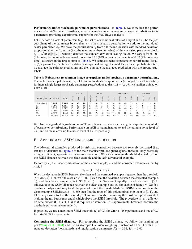
Performance under stochastic parameter perturbations In Table 4, we show that the perfor-mance of an AdA-trained classifier gradually degrades under increasingly larger perturbations to itsparameters, providing experimental support for the PAC-Bayes analysis.

Let w denote a block of parameters (e.g., the set of convolutional filters of a layer) and wj be the j-thcoordinate of the parameter block; then, εj is the stochastic perturbation we add to the individualscalar parameter wj . We draw the perturbation εj from a 0-mean Gaussian with standard deviationproportional to the `∞ norm (i.e., the maximum absolute value) of the enclosing parameter block:εj ∼ N (0, η ‖w‖∞) , where η denotes the standard deviation scaling factor. We vary η from 0.00(0% noise; i.e., nominally evaluated model) to 0.10 (10% noise) in increments of 0.02 (2% noise at atime), as shown in the first column of Table 4. We sample stochastic parameter perturbations (for allof fθ’s parameters) 50 times per dataset example and average the model’s predicted probabilities (i.e.,we average the softmax predictions and then compare the averaged prediction with the ground-truthlabel).

Table 4: Robustness to common image corruptions under stochastic parameter perturbations.The table shows top-1 clean error, mCE and individual corruption error (averaged over all severities)for increasingly larger stochastic parameter perturbations to the AdA + AUGMIX classifier trained onCIFAR-10.

NOISE BLUR WEATHER DIGITAL

NOISE (%) CLEAN E MCE

GA

US

S

SH

OT

IMP

UL

SE

DE

FO

CU

S

GL

AS

S

MO

TIO

N

ZO

OM

SN

OW

FR

OS

T

FO

G

BR

IGH

T

CO

NT

RA

ST

EL

AS

TIC

PIX

EL

JPE

G

0% (default) 3.74% 8.80% 16.4 12.8 14.4 5.7 10.9 7.5 6.3 7.7 6.7 6.6 3.9 4.7 8.1 11.9 8.4

2% 3.76% 8.81% 16.5 12.8 14.5 5.7 10.9 7.6 6.4 7.7 6.7 6.6 3.9 4.8 8.1 11.8 8.3

4% 3.75% 9.21% 17.4 13.4 15.2 6.2 11.4 8.2 6.9 7.9 6.9 6.8 4.0 5.6 8.2 11.7 8.3

6% 4.28% 10.49% 19.5 15.1 17.2 7.3 12.8 9.8 8.5 8.6 7.7 7.8 4.4 8.5 9.0 12.4 8.9

8% 6.01% 14.56% 24.5 19.4 22.9 11.2 17.9 14.7 12.6 11.6 10.1 11.3 6.4 15.8 12.3 16.2 11.4

10% 17.75% 31.34% 40.7 35.5 44.5 26.9 40.9 34.5 30.2 29.0 22.2 24.9 19.2 34.2 28.2 32.8 26.2

We observe a gradual degradation in mCE and clean error when increasing the expected magnitudeof parameter perturbations. Performance on mCE is maintained up to and including a noise level of2%, and on clean error up to a noise level of 4% respectively.

F APPROXIMATE SSIM LINE-SEARCH PROCEDURE

The adversarial examples produced by AdA can sometimes become too severely corrupted (i.e.,left-tail of densities in Figure 2 of the main manuscript). We guard against these unlikely events byusing an efficient, approximate line-search procedure. We set a maximum threshold, denoted by t, onthe SSIM distance between the clean example and the AdA adversarial example.

Denote by xγ the linear combination of the clean example, x, and the corrupted example output byAdA, x:

xγ = (1− γ)x+ γ x.

When the deviation in SSIM between the clean and the corrupted example is greater than the threshold(SSIM(x, x) > t), we find a scalar γ∗ ∈ [0, 1] such that the deviation between the corrected example,x∗γ , and the clean example, x, is t: SSIM(x, x∗γ) = t. We take 9 equally-spaced γ values in [0, 1]and evaluate the SSIM distance between the clean example and xγ for each considered γ. We fit aquadratic polynomial in γ to all the pairs of γ and the threshold-shifted SSIM deviation from theclean example SSIM(x, xγ)− t. We then find the roots of this polynominal, clip them to [0, 1], andtake the γ closest to 1 as the desired γ∗. This corresponds to returning the most corrupted variant ofx along the ray between x and x which obeys the SSIM threshold. The procedure is very efficienton accelerators (GPUs, TPUs) as it requires no iteration. It is approximate, however, because thequadratic polynomial can underfit.

In practice, we use a maximum SSIM threshold (t) of 0.3 for CIFAR-10 experiments and one of 0.7for IMAGENET experiments.

Computing the SSIM distance. For computing the SSIM distance we follow the original pa-per (Wang et al., 2004) and use an isotropic Gaussian weighting function of 11 × 11 with a 1.5standard deviation (normalized), and regularization parameters K1 = 0.01, K2 = 0.03.

21

G ADDITIONAL EXPERIMENTS AND COMPARISONS

Comparison to previous work on CIFAR-10. Perceptual Adversarial Training (PAT) (Laidlawet al., 2021) proposes an adversarial training method based on bounding a neural perceptual distance(LPIPS). Appendix G (Table 10) of the PAT article shows the performance of various models oncommon image corruptions. However, performance is summarized using relative mCE, whereas weuse absolute mCE throughout. The authors kindly provided us6 with the raw corruption errors oftheir models at each severity and we reproduce their results in (the top half of) Table 5. We observethat PAT has overall lower robustness to common image corruptions (best variant obtains 23.54%mCE) than AugMix (10.90% mCE) and than our best AdA-trained model (7.83% mCE).

PAT however, performs very well against other adversarial attacks7, including `p-norm boundedperturbations. The best PAT model obtains 28.7% robust accuracy against `∞ attacks (ε = 8/255)and 33.3% on `2 attacks (ε = 1) while our best AdA-variant obtains less robust accuracy in eachcase (0.99% against `2 attacks and 13.88% against `∞ attacks with ε = 4/255). This difference inperformance against `p-norm attacks is not surprising, as PAT addresses robustness to pixel-levelattacks (i.e., it manipulates image pixels directly); whereas AdA applies adversarial perturbations tothe corruption function parameters (and not to the image pixels directly).

In similar spirit to PAT, Kireev et al. (2021) introduce an efficient relaxation of adversarial trainingwith LPIPS as the distance metric. Their best model, with a smaller architecture, RESNET18, obtains11.47% mCE on CIFAR-10-C. The authors of Kireev et al. (2021) also show that models trainedadversarially against `p-norm bounded perturbations can act as a strong baseline for robustness tocommon image corruptions.

The strongest known8 adversarially trained model against `p-norm bounded perturbations on commonimage corruptions is that of Gowal et al. (2020) which obtains 12.32% mCE (training against `2-normbounded perturbations with ε = 0.5 while using extra-data).

In Wong & Kolter (2021a), the authors first train generative models to represent image corruptionsby feeding them a subset of the common image corruptions (from CIFAR-10-C). In a second stage,they train classifiers using samples (adversarial or random) coming from these pre-trained generativemodels. Despite having this additional knowledge of the test set corruptions, the robust classifiersthey train only achieve between 9.5% and 9.7 mCE%.

To the best of our knowledge, our best performing model (AdA (EDSR) coupled with AugMix andDeepAugment) is more robust to common image corruptions on CIFAR-10 than all previous methods,obtaining a new state-of-the-art mCE of 7.83%.

Table 5: Performance of Perceptual Adversarial Training on common image corruptions. Thetable lists the performance of ResNet50 models trained using Perceptual Adversarial Training bythe original authors of Laidlaw et al. (2021) on common image corruptions and two of our AdA-trained models. The table shows clean error, mean corruption error on CIFAR-10-C and individualcorruption errors for each corruption type (averaged across all severities). “PAT-self” denotes thecase where the same model is used for classification as well as for computing the LPIPS distance,while “PAT-AlexNet” denotes the case where the LPIPS distance is computed using a pre-trainedCIFAR-10 AlexNet (Krizhevsky et al., 2012) classifier.


SETUP CLEAN E MCE

GA

US

S

SH

OT

IMP

UL

SE

DE

FO

CU

S

GL

AS

S

MO

TIO

N

ZO

OM

SN

OW

FR

OS

T

FO

G

BR

IGH

T

CO

NT

RA

ST

EL

AS

TIC

PIX

EL

JPE

G

PAT MODELS (LAIDLAW ET AL., 2021)Nominal Training 5.20% 25.80% 54.0 42.3 38.8 16.5 50.9 21.9 21.1 18.3 24.0 10.5 6.1 16.0 17.6 28.2 20.7

Adversarial Training `∞ 13.20% 20.71% 18.3 17.0 22.5 16.9 19.8 20.4 17.5 17.0 18.2 32.9 13.7 47.9 18.1 15.0 15.3

Adversarial Training `2 15.00% 21.83% 18.4 17.5 21.4 18.3 20.2 21.0 18.7 19.2 20.5 35.9 16.0 47.1 20.0 16.6 16.5

PAT-self 17.60% 23.54% 22.5 21.1 25.7 20.0 22.5 22.2 20.3 23.7 23.6 33.5 19.8 38.8 21.7 18.7 19.1

PAT-AlexNet 28.40% 34.25% 33.2 31.9 36.3 30.9 34.3 33.0 32.0 33.9 35.0 43.7 30.5 46.5 32.6 29.9 29.8

SELECTION OF AdA MODELS (OURS)AdA (EDSR) 6.63% 15.47% 27.3 21.5 31.7 11.8 20.0 13.9 14.1 12.9 11.5 11.8 7.0 14.9 12.7 9.4 11.5

AdA (EDSR) + DeepAugment + AugMix 5.07% 7.83% 8.8 7.8 11.2 5.9 10.7 7.3 6.5 8.5 6.7 8.7 5.2 6.2 8.5 7.7 7.8

6Personal communication.7See Table 2 of Laidlaw et al. (2021) for full details.8See the ROBUSTBENCH (Croce et al., 2020) leaderboard: https://robustbench.github.io.

22

https://robustbench.github.io

Number of inner optimization steps. We show the effect of changing the number of inner op-timization steps (i.e. the number of PGD steps for finding adversarial examples) for AdA (EDSR)on CIFAR-10 in Table 6. We sweep a number of PGD steps from 0 to 10 where 10 is the defaultfor CIFAR-10. As described in section D, we compensate for the decrease in number of PGD steps(from 10) by proportionally scaling up the step size (i.e. effective ηc = ηc·10

num steps ). Zero (0) PGDsteps correspond to only performing the random initialization of perturbations to the corruptionnetwork’s parameters (i.e. lines 5-6 in Algorithm 1). We observe that performance on common imagecorruptions in aggregate (mCE) and for individual groups, in general, increases with the number ofinner optimization PGD steps. We note that adversarial training appears to be necessary for trainingthe most robust models, and randomly sampling the parameter perturbations is not sufficient.

Table 6: Effect of number of inner optimization steps on robustness to common image corrup-tions (CIFAR-10-C). The table shows the performance of the AdA (EDSR) model while varying thenumber of inner optimization steps (M ). The table shows the clean top-1 error, the mean corruptionerror on CIFAR-10-C and on individual corruptions (averaged across all severities).


NUM. PGD STEPS CLEAN E MCE

GA

US

S

SH

OT

IMP

UL

SE

DE

FO

CU

S

GL

AS

S

MO

TIO

N

ZO

OM

SN

OW

FR

OS

T

FO

G

BR

IGH

T

CO

NT

RA

ST

EL

AS

TIC

PIX

EL

JPE

G

0 (i.e. only random init.) 8.99 28.35 43.4 34.1 35.3 22.6 49.9 30.0 29.1 22.9 24.6 16.3 10.5 28.2 23.6 31.0 23.6

2 7.87 17.91 21.5 18.3 28.5 18.8 27.5 17.7 23.7 16.0 15.4 11.3 8.5 12.6 18.6 14.0 16.4

4 6.99 14.91 26.2 21.0 25.8 12.0 18.6 12.9 14.7 12.8 11.7 11.6 7.4 13.7 13.4 9.8 12.0

6 6.83 15.94 30.2 23.7 29.8 12.1 19.2 13.7 15.4 13.0 12.2 12.8 7.2 15.1 13.3 9.5 11.9

8 6.80 15.66 28.0 22.4 30.5 12.6 18.4 14.3 15.0 12.7 11.9 12.2 7.3 15.1 13.0 9.7 12.0

10 6.63 15.47 27.3 21.5 31.7 11.8 20.0 13.9 14.1 12.9 11.5 11.8 7.0 14.9 12.7 9.4 11.5

Perturbation radius. We show the effect of changing the corruption network parameters perturba-tion radius in AdA on CIFAR-10 in Table 7. We perform a sweep on the perturbation radius by scalingthe radius (ν = 0.015) of the best performing model, AdA (EDSR) + DeepAugment + AugMix(from Table 1 in the main manuscript), by {0.5, 0.75, 1.0, 1.25, 1.5}. We observe that the robustnessperformance varies minimally across a small range of perturbation radii.

Table 7: Effect of perturbation radius on robustness to common image corruptions (CIFAR-10-C). The table shows the performance of the best AdA-combination from Table 1 from the mainmanuscript (AdA (EDSR) + DeepAugment + AugMix) while varying the perturbation radius (ν).The table shows mean corruption error on CIFAR-10-C and individual corruption errors for eachcorruption type (averaged across all severities).


PERTURBATION RADIUS MCE

GA

US

S

SH

OT

IMP

UL

SE

DE

FO

CU

S

GL

AS

S

MO

TIO

N

ZO

OM

SN

OW

FR

OS

T

FO

G

BR

IGH

T

CO

NT

RA

ST

EL

AS

TIC

PIX

EL

JPE

G

ν = 0.0225 8.10% 9.4 8.1 11.5 6.2 11.4 7.5 6.6 8.8 6.9 8.5 5.5 6.4 8.8 7.8 8.1

ν = 0.01875 8.06% 8.8 7.9 11.5 6.1 11.2 7.6 6.5 9.0 7.0 8.7 5.5 6.5 8.8 7.6 8.1

ν = 0.015 (default) 7.83% 8.8 7.8 11.2 5.9 10.7 7.3 6.5 8.5 6.7 8.7 5.2 6.2 8.5 7.7 7.8

ν = 0.01125 8.41% 9.1 8.3 12.1 6.5 11.3 8.0 6.8 9.2 7.2 9.2 5.8 6.8 9.2 8.1 8.5

ν = 0.0075 7.99% 8.9 8.0 11.0 6.2 10.7 7.7 6.2 9.0 6.9 8.6 5.5 6.9 8.7 7.6 8.1

Performance on image corruptions through training. We visualize the performance of AdAtrained models (best AdA-combination from Table 1 and Table 2 from the main manuscript) duringtraining in Figure 4. Due to adversarial training, we expect the performance on each of the *-Ccorruptions to improve as training progresses, and this is indeed what we observe. On both datasets,the AdA-trained classifiers perform consistently best on Brightness, especially at the beginning oftraining. On IMAGENET performance increases more slowly on the Blur-type corruptions than on allothers.

Extended results on individual image corruptions. We provide supplemental details to Tables 1and 2 (from the main manuscript) on individual corruption types in Table 8 and Table 9, respectively.

23

0 25 50 75 100Training progress (%)

Gaussian Noise

Shot Noise

Impulse Noise

Defocus Blur

Frosted Glass Blur

Motion Blur

Zoom Blur

Snow

Frost

Fog

Brightness

Contrast

Elastic

Pixelate

JPEG Compression

Gaussian Blur

Saturate

Spatter

Speckle Noise

Accuracy


Column-normalized accuracy (each column sums to 1)


Row-normalized accuracy (each row sums to 1)

(a) CIFAR-10


Gaussian Noise

Shot Noise

Impulse Noise

Defocus Blur

Glass Blur

Motion Blur

Zoom Blur

Snow

Frost

Fog

Brightness

Contrast

Elastic Transform

Pixelate

JPEG Compression

Gaussian Blur

Spatter

Speckle Noise

Accuracy


Column-normalized accuracy (each column sums to 1)


Row-normalized accuracy (each row sums to 1)

(b) IMAGENET

Figure 4: Performance on image corruptions through training. These plots visualize the perfor-mance of the best AdA combination on each of the common and extra *-C corruptions as trainingprogresses. Each individual rectangle plots top-1 accuracy. Brighter is better. The accuracies arevisualized raw (plots to the left), normalized over the columns (middle plots) or over the rows (plotsto the right). Normalizing over the columns visualizes which corruption’s performance is best at thatpoint in training. Normalizing over the rows visualizes at which stage the classifier performs best ona given corruption.

24

Table 8: CIFAR-10: Extended results on robustness to common image corruptions. The tableshows mean corruption error on CIFAR-10-C and individual corruption errors for each corruptiontype (averaged across all 5 severities).


SETUP MCE

GA

US

S

SH

OT

IMP

UL

SE

DE

FO

CU

S

GL

AS

S

MO

TIO

N

ZO

OM

SN

OW

FR

OS

T

FO

G

BR

IGH

T

CO

NT

RA

ST

EL

AS

TIC

PIX

EL

JPE

G

WITHOUT ADDITIONAL DATA AUGMENTATION:Nominal 29.37 49.8 39.5 39.5 20.1 53.2 27.8 26.8 24.1 27.8 17.0 10.1 28.6 21.2 31.9 23.0

AdA (U-Net) 23.11 40.4 33.1 35.9 16.8 41.5 18.9 21.2 19.8 20.9 13.5 7.9 17.2 17.7 23.6 18.2

AdA (VQ-VAE) 26.77 25.1 24.3 28.9 23.8 26.8 25.9 25.1 27.7 24.9 37.1 22.6 37.1 26.7 22.8 22.6

AdA (EDSR) 15.47 27.3 21.5 31.7 11.8 20.0 13.9 14.1 12.9 11.5 11.8 7.0 14.9 12.7 9.4 11.5

AdA (CAE) 29.15 26.5 26.3 28.2 25.2 28.0 27.1 26.4 31.3 28.5 40.9 25.9 43.0 29.1 25.5 25.4

AdA (All) 18.49 20.6 18.6 23.4 16.3 23.7 18.6 18.9 18.6 17.4 19.7 12.2 20.8 18.2 15.1 15.4

AT (`∞) 23.64 18.6 17.5 25.6 18.6 20.2 22.8 19.4 20.8 24.9 40.1 17.7 56.2 20.0 15.8 16.2

AT (`2) 17.42 12.8 11.7 17.2 13.5 16.0 17.2 14.2 15.7 16.4 33.9 11.3 44.8 14.8 10.8 10.8

TRADES (`∞) 24.72 19.8 18.7 25.4 20.0 21.5 23.6 20.8 22.2 26.5 40.9 19.4 56.2 21.2 17.2 17.4

TRADES (`2) 18.08 13.0 12.3 16.9 14.2 16.1 17.6 14.7 16.9 17.9 34.4 12.7 45.3 15.6 11.9 11.7

AWP (`∞) 25.01 20.4 19.2 25.7 20.1 21.7 23.5 21.0 22.6 27.6 40.4 20.2 56.1 21.4 17.7 17.8

AWP (`2) 18.79 14.1 13.1 17.6 14.5 16.4 17.5 15.2 17.8 19.3 35.3 13.7 46.7 15.9 12.5 12.4

SAM 24.59 58.5 43.8 46.0 14.7 46.8 19.4 18.0 15.2 19.8 11.0 5.2 20.5 13.0 20.5 16.4

WITH AUGMIX:Nominal 12.26 27.3 20.2 15.9 7.7 14.4 10.7 9.4 9.2 9.4 7.2 4.5 6.0 9.8 20.6 11.6

AdA (U-Net) 12.02 24.6 18.8 18.2 7.2 16.3 9.1 8.7 10.1 9.9 7.8 4.4 5.3 10.0 19.4 10.3

AdA (VQ-VAE) 20.85 22.4 21.2 25.6 19.0 24.3 19.4 19.1 22.0 20.0 24.4 16.7 20.2 20.3 19.9 18.3

AdA (EDSR) 9.40 17.3 13.7 16.5 6.2 11.9 8.1 7.1 8.5 7.6 7.6 4.2 5.3 8.7 10.3 8.0

AdA (CAE) 20.20 19.3 18.5 22.6 17.1 22.9 19.6 18.0 22.6 20.0 26.0 16.6 21.4 20.5 20.1 17.8

AdA (All) 14.12 18.8 16.3 17.9 12.8 17.0 13.8 14.1 13.8 12.5 12.9 8.4 10.6 13.6 16.6 12.8

WITH DEEPAUGMENT:Nominal 11.94 12.5 11.1 15.0 8.6 18.7 11.7 9.9 12.7 10.5 10.1 7.9 10.9 13.0 14.3 12.1

AdA (U-Net) 13.09 13.7 12.6 19.5 10.0 19.4 12.1 11.1 14.4 11.2 13.0 8.9 9.8 14.1 13.8 12.8

AdA (VQ-VAE) 26.35 29.8 28.4 32.9 22.7 26.6 24.7 23.3 27.8 25.2 32.6 22.7 26.5 26.1 23.1 23.0

AdA (EDSR) 12.37 13.0 12.0 17.7 10.0 16.1 11.8 10.7 13.3 10.9 13.2 9.1 11.4 13.6 10.8 11.9

AdA (CAE) 27.98 26.9 26.6 28.4 25.8 28.4 27.1 26.6 30.3 27.4 36.3 25.2 29.5 29.2 25.8 26.1

AdA (All) 21.70 21.5 20.6 23.9 20.1 24.9 22.4 21.4 23.4 20.4 25.7 18.1 20.1 23.1 19.9 19.9

WITH AUGMIX & DEEPAUGMENT:Nominal 7.99 8.9 7.5 10.0 5.4 11.4 7.7 6.1 8.5 6.5 7.2 4.9 6.3 8.2 12.3 8.8

AdA (U-Net) 8.63 9.4 8.2 11.9 5.9 12.6 7.7 6.6 9.2 6.8 8.6 5.0 5.9 9.1 14.0 8.5

AdA (VQ-VAE) 25.17 26.1 25.5 29.2 22.3 27.6 23.8 22.5 27.1 25.4 30.1 22.9 23.6 25.0 23.0 23.2

AdA (EDSR) 7.83 8.8 7.8 11.2 5.9 10.7 7.3 6.5 8.5 6.7 8.7 5.2 6.2 8.5 7.7 7.8

AdA (CAE) 20.09 19.2 18.6 21.2 17.3 23.1 20.4 18.1 22.6 20.1 26.4 16.8 19.8 20.4 19.5 18.0

AdA (All) 11.72 12.0 11.1 14.3 10.2 14.7 11.5 10.6 13.0 10.5 13.7 8.3 9.6 12.2 12.2 11.7

25

Table 9: IMAGENET (128×128): Extended results on robustness to common image corruptions.The table shows mean corruption error on IMAGENET-C and individual corruption errors for eachcorruption type (averaged across all 5 severities).


SETUP MCE

GA

US

S

SH

OT

IMP

UL

SE

DE

FO

CU

S

GL

AS

S

MO

TIO

N

ZO

OM

SN

OW

FR

OS

T

FO

G

BR

IGH

T

CO

NT

RA

ST

EL

AS

TIC

PIX

EL

JPE

G

WITHOUT ADDITIONAL DATA AUGMENTATION:Nominal 82.40 73.2 74.8 80.1 71.4 78.5 70.4 65.4 66.7 63.6 46.1 35.8 63.3 57.4 72.4 55.9

AdA (U-Net) 83.51 81.2 81.7 92.8 79.0 86.2 73.0 74.4 61.3 60.7 41.6 34.2 48.4 65.9 51.3 58.7

AdA (VQ-VAE) 78.26 73.7 71.9 72.4 71.5 66.1 62.6 66.9 67.0 63.8 60.1 44.3 64.7 54.7 44.9 43.6

AdA (EDSR) 79.59 74.9 75.4 78.0 70.1 75.0 67.9 66.3 62.9 60.0 44.4 33.6 56.7 57.4 64.8 54.9

AdA (CAE) 86.44 89.6 89.2 94.4 75.8 70.3 68.3 66.8 75.5 68.3 56.4 45.1 65.3 55.1 62.1 47.8

AdA (All) 75.03 76.3 76.4 83.1 67.8 72.9 65.8 67.5 59.0 55.7 41.9 31.7 48.5 57.4 37.8 50.8

WITH AUGMIX:Nominal 77.12 70.4 71.6 75.6 67.2 75.1 64.0 59.0 60.9 61.1 37.9 34.7 46.9 57.5 71.4 55.9

AdA (U-Net) 77.87 71.2 72.1 86.5 74.0 81.4 66.1 64.6 57.8 58.1 37.5 32.9 41.4 65.4 51.0 59.3

AdA (VQ-VAE) 73.41 75.1 73.7 69.3 68.3 69.5 61.1 60.0 61.8 56.3 41.7 38.1 44.0 56.6 44.5 48.1

AdA (EDSR) 73.59 67.3 68.2 71.7 65.6 73.8 62.8 61.1 61.3 58.7 39.6 31.9 43.2 55.6 60.8 48.5

AdA (CAE) 80.85 87.4 86.6 91.2 66.7 65.7 63.0 63.0 71.3 66.0 50.6 42.2 52.2 53.5 59.1 44.6

AdA (All) 72.27 66.9 66.6 71.4 67.7 71.5 60.4 60.6 58.2 55.3 39.7 33.0 40.5 58.8 46.4 55.2

WITH DEEPAUGMENT:Nominal 73.04 52.1 52.1 53.3 60.5 69.0 65.9 63.3 57.7 55.4 43.8 33.8 58.2 56.2 66.8 63.8

AdA (U-Net) 75.03 54.6 56.3 60.0 67.5 77.5 66.7 72.0 55.9 54.8 40.7 34.8 42.1 62.6 47.0 79.5

AdA (VQ-VAE) 69.15 56.7 58.7 56.8 57.8 63.5 61.6 68.7 57.2 54.4 46.2 37.2 49.8 57.4 37.3 49.3

AdA (EDSR) 65.62 48.2 49.7 48.8 58.4 66.3 62.3 63.4 56.8 53.4 42.6 31.0 50.9 53.3 33.7 51.7

AdA (CAE) 77.55 64.2 66.9 69.6 64.3 73.8 66.9 66.7 56.5 55.2 44.6 36.7 50.2 61.5 39.3 87.3

AdA (All) 65.54 47.1 48.3 47.9 59.2 66.4 60.4 65.2 54.2 51.3 42.5 32.5 44.2 55.4 37.4 54.2

WITH AUGMIX & DEEPAUGMENT:Nominal 70.05 50.5 50.0 51.5 58.0 67.8 60.1 58.7 54.5 53.3 37.5 33.4 43.6 56.8 64.2 72.0

AdA (U-Net) 71.64 53.9 54.5 57.8 62.3 73.3 63.1 65.9 53.7 53.2 38.1 34.2 38.0 61.8 45.8 76.0

AdA (VQ-VAE) 69.02 54.2 54.6 54.0 56.8 62.9 59.2 66.2 58.3 56.0 47.7 42.0 47.6 59.5 42.0 46.7

AdA (EDSR) 64.31 47.6 48.1 48.5 55.3 64.5 56.8 56.8 55.0 52.0 39.8 32.1 41.2 54.3 35.1 62.2

AdA (CAE) 67.89 55.8 56.1 55.2 55.6 62.1 59.4 60.9 57.2 55.5 45.8 39.1 45.7 59.7 38.5 48.5

AdA (All) 62.90 48.1 48.4 48.9 55.4 63.7 54.7 60.2 53.3 51.1 41.0 34.1 39.6 56.1 36.3 45.4

26

deepmind - arxiv.org

Documents