PORTFOLIO SELECTION WITH MULTIPLE SPECTRAL RISKCONSTRAINTS

CARLOS ABAD∗ AND GARUD IYENGAR†

Abstract. We propose an iterative gradient-based algorithm to efficiently solve the portfolioselection problem with multiple spectral risk constraints. Since the conditional value at risk (CVaR)is a special case of the spectral risk measure, our algorithm solves portfolio selection problems withmultiple CVaR constraints. In each step, the algorithm solves very simple separable convex quadraticprograms; hence, we show that the spectral risk constrained portfolio selection problem can be solvedusing the technology developed for solving mean-variance problems. The algorithm extends to thecase where the objective is a weighted sum of the mean return and either a weighted combinationor the maximum of a set of spectral risk measures. We report numerical results that show that ourproposed algorithm is very efficient; it is at least one order of magnitude faster than the state-of-the-art general purpose solver for all practical instances. One can leverage this efficiency to be robustagainst model risk by including constraints with respect to several different risk models.

Key words. large scale portfolio optimization, coherent risk measures, first-order algorithms

AMS subject classifications. 90C90, 90B50, 91G10

1. Introduction. Portfolio selection is concerned with distributing a given cap-ital over a finite number of investment opportunities in order to maximize “return”while managing “risk”. Although, the benefits of diversification to manage “risk” hadbeen long known, Markowitz [1952] was the first to propose a mathematical modelfor the portfolio optimization problem, representing “return” by the expected returnof the portfolio, and “risk” by the variance in the return of the portfolio. It has beenobserved that variance is a good measure of risk only if the returns are ellipticallydistributed. Moreover, since variance is not sensitive to the tails of the distribution,it is not a good measure of variability when the returns are heavy tailed.

A number of risk measures have been proposed in the literature to accommodateasymmetry and also capture the effects of heavier tails. The Value-at-Risk VaRβ(L)

at the probability level β for a random loss L is defined as the β quantile of the lossdistribution, i.e. the probability of observing losses larger than VaRβ(L) is at most1 − β [Jorion, 2006]. VaR is extensively used in risk management applications, andit is the mandated risk measure in the Basel-II accords. However, it has a number ofshortcomings. First, VaR only depends on the probability of tail losses and not theirlocation in the tail. Second, VaR is not a convex risk measure; consequently, portfolioselection with VaR constraints often results in integer programs that are hard to solve.

Conditional Value-at-Risk CVaRβ(L) = E[L | L ≥ VaRβ ] [Rockafellar and Urya-

sev, 2000] and Expected Shortfall ESβ = 11−β

∫ 1

βVaRp(L)dp [Acerbi and Tasche,

2002] are closely related risk functions that address the two shortcomings of VaRlisted above. CVaR and ES are both coherent risk measures [Artzner et al., 1999],i.e. they are convex and positively homogeneous. Acerbi and Tasche [2002] showedthat the ES of a portfolio can be estimated from samples of the losses on the un-derlying assets by solving a linear program (LP), and that the estimate converges tothe ES of the portfolio with probability 1. Rockafellar and Uryasev [2000] showed asimilar result for CVaR assuming that the loss distribution of the portfolio is con-

∗IEOR, Columbia University. ca2446@columbia.edu†IEOR, Columbia University. Supported in part by NSF grants DMS-1016571, DOE grant DE-

FG02-08ER25856 and ONR grant N000140310514

1

arX

iv:1

410.

5328

v2 [

q-fi

n.PM

] 2

5 M

ar 2

015

tinuous at the β quantile. Acerbi [2002] extended ES to the spectral risk measure

Mφ(L) =∫ 1

0VaRp(L)φ(p)dp, where φ(p) is a non-increasing probability distribution

function. The spectral risk measure Mφ(L) is coherent and, in fact, ESβ(L) = Mφ(L)

with φ(p) = 11−β1β≤p≤1. Acerbi [2002] also showed that the finite sample estimate

MNφ =

∑Nk=1 φ( kN )L(N−k), where L(k) denotes the k-th order statistic of N inde-

pendent and identically distributed (IID) samples of the random loss L, converges toMφ(L) with probability 1.

From Acerbi [2002], it follows that the portfolio selection problem where the“return” is given by the expected return of the portfolio and the “risk” is given by aspectral risk measure of the portfolio can be approximated by an LP. Rockafellar andUryasev [2000] established such an LP-based approximation result for the mean-CVaRportfolio selection problem. Agarwal and Naik [2004] showed that the mean-CVaRportfolio selection results in superior portfolios as compared to the mean-varianceapproach when the risk of the assets is nonlinear in the underlying risk factors, e.g.when the asset is a derivative written on a primary asset. However, the resultingLP is very ill-conditioned, and solving such LP, particularly when the scenario size islarge, is very difficult in practice (see, e.g. [Alexander et al., 2006]). Lim et al. [2011]showed that the solution of the mean-CVaR portfolio problem is often very sensitiveto estimation errors, i.e. small errors in the estimation of the mean and the return inthe scenarios can get amplified in the choice of the optimal portfolio. This sensitivitycan be addressed by imposing spectral risk constraints with respect to several differentparameter values and also different risk models. Constraints with respect to multiplerisk models have become especially important after the 2008 financial crisis (see, e.g.[Ceria et al., 2009]). However, imposing multiple spectral risk constraints increasesthe size of the LP by such an extent that state-of-the-art solvers are unable to solvemost practical instances of the portfolio selection problem.

Our contributions in this paper are as follows:

(a) We propose a new first-order gradient based algorithm SpecRiskAllocate tosolve portfolio selection problems with multiple spectral risk constraints that issignificantly faster than the naive LP-based approach. We exploit two key fea-tures of the portfolio selection problem to construct this algorithm. The first isthat the constraints in the LP formulation (2.3) are very loosely coupled in thatthe samples from a particular risk model only play a role in the correspondingconstraint. Thus, one can improve the run time of the algorithm by dualizingthese constraints, provided feasibility is maintained. We show in Theorem (3.1)that we are able to recover feasible portfolios for finite values of the dual vari-ables. The second feature we exploit is that, since the LP is in fact a finite sampleapproximation to the stochastic optimization problem, in practice one is not at-tempting to solve it to very high accuracy (e.g. 10−12 relative error) but ratherone is satisfied with moderate accuracy (e.g. 10−3 relative error). This allowsus to smooth the LP into a smooth convex optimization problem, resulting insignificantly faster convergence.

(b) SpecRiskAllocate computes the optimal portfolio by solving a sequence ofsmall separable convex quadratic programs (QPs). Thus, portfolio managerswould be able to solve spectral risk constrained portfolio selection problems usingexisting tools for solving mean-variance problems. The number of variables ineach of the convex QPs is equal to the number of assets and, therefore, theseproblems can be solved very efficiently. In some cases, the optimal solution of the

2

mean-variance subproblem can be written in closed form or computed by a onedimensional search. SpecRiskAllocate is also able to solve portfolio selectionproblems where the objective is to maximize a weighted sum of the expected re-turn and either a weighted combination or the maximum of a set of spectral riskmeasures.

(c) The experimental results in Section 4 clearly show that SpecRiskAllocateis able to efficiently solve very large spectral risk constrained portfolio selectionproblems. For most practical instances, SpecRiskAllocate is at least one orderof magnitude faster than the state-of-the-art LP solvers. Moreover, we show that,in contrast to the LP-based method, SpecRiskAllocate is not ill-conditioned.This is a side-benefit of smoothing the problem. “Smoothing” approximates theLP polytope by a convex set without corners; thus, ensuring that the optimalsolution is a continuous function of the problem and, therefore, not ill-conditioned.

(d) A popular method for introducing robustness against model uncertainty is to im-pose spectral risk constraints with respect to several risk models (see e.g. Brownand Canova [2011] and Renshaw [2012]). In Section 4, we show that SpecRisk-Allocate is able to solve a hedging portfolio selection problem with spectral riskconstraints corresponding to multiple risk models in a computationally tractablemanner.

SpecRiskAllocate is based on the proximal gradient algorithm FISTA proposedby Beck and Teboulle [2009] (see also Nesterov [2005]). The algorithm we propose issimilar to the one proposed by Iyengar and Ma [2013] in that both these algorithms useNesterov smoothing techniques [Nesterov, 2005]. However, there are a number of keydifferences between the two methods. The algorithm in Iyengar and Ma [2013] is onlyable to solve a mean-CVaR problem and can be extended to solve a mean-weightedCVaR problem; however, it is not able to compute solutions for portfolio selectionproblems with CVaR (or, more generally, spectral risk) constraints. SpecRickAllo-cate uses a different smoothing technique that allows us to scale the algorithm tosolve very large portfolio selection problems without encountering any numerical dif-ficulty. Iyengar and Ma [2013] were unable to solve large problem instances becausethe algorithm proposed therein quickly becomes numerically unstable.

The rest of this paper is organized as follows. In Section 2 we introduce thegeneralized spectral risk measures and define the generalized spectral risk constrainedportfolio selection problem. In Section 3 we construct the SpecRiskAllocate algo-rithm. In Section 4 we discuss the results of our numerical experiments. Finally, inSection 5 we conclude with some final remarks.

2. Single period portfolio selection problem. Suppose there are n assets

in the market. Let L =(L1, . . . , Ln

)>∈ Rn denote the random rate of loss on the

assets. Let x ∈ Rn denote the portfolio of the investor, i.e., 1>x =∑ni=1 xi = 1. The

rate of loss Lx of portfolio x is given by Lx = L>

x. In this paper, we want to identifyportfolios that lie on the Pareto optimal frontier with respect to the expected return−E[Lx] and a set of generalized spectral risk measures [Acerbi, 2002].

Except for some special cases –e.g. when the random loss vector L is a linearfunction of the distribution of elliptically distributed risk factors Z– the distributionof the random portfolio loss Lx is hard to characterize explicitly. This is definitely thecase if the portfolio x contains derivative securities whose distribution is nonlinear inthe underlying risk factors. In practice, L is approximated by N samples `1, . . . , `Ngenerated by some scenario generator (see, e.g. Koskosidis and Duarte [1997]). Let

3

L = (`1, . . . , `N )> ∈ RN×n denote the empirical loss matrix, where the j-th column

represents the vector of N loss realizations of asset j. Thus, the random loss Lx on theportfolio x can be approximated by the set of samples `>1 x, . . . , `>Nx or, equivalently,by the vector Lx. In the rest of this section, we define the generalized spectral lossfunction for the vector Lx and relate it to the Expected Shortfall measure. Thisrelation will be important for designing our solution algorithm in Section 3.

2.1. Generalized spectral risk measures. Let y = (y1, . . . , yN )> denote Nsamples of a random variable Y . Let y(`) : ` = 1, . . . , N denote the order statisticsof vector y.

Definition 2.1 (Expected shortfall (ES) [Acerbi and Tasche, 2002]). The ex-pected shortfall of y at level β ∈ [0, 1) is the average of the κ = d(1 − β)Ne largestvalues of y, i.e.,

ESβ(y) =1

κ

N∑`=N−κ+1

y(`).

It is easy to check that ESβ(y) has the following variational characterization (see,e.g. Artzner et al. [1999], Rockafellar et al. [2002], Luthi and Doege [2005]) :

ESβ(y) = max∑N`=1 q`y`,

such that 1>q = 1,0 ≤ q ≤ 1

κ · 1.

Using linear programming duality [Bertsimas and Tsitsiklis, 1997] it follows that

(2.1) ESβ(y) = minz

z +

1

κ·N∑`=1

(y` − z)+

,

where v+ = maxv, 0. Acerbi and Tasche [2002] established that ESβ(·) is a coherentrisk measure [Artzner et al., 1999] and converges to CVaR [Rockafellar et al., 2002,Luthi and Doege, 2005] when the cumulative distribution function FY (·) of the randomvariable Y is continuous at y = infx : FY (x) ≥ β.

Definition 2.2 (Spectral risk measure [Acerbi, 2002]). Let ω = (ω1, . . . , ωN )>

denote a non-decreasing probability mass function, i.e. ω ≥ 0, 1>ω = 1, and ωk ≥ ω`whenever k ≥ `. The spectral risk measure Mω(y) generated by ω is defined as

Mω(y) =

N∑`=1

ω`y(`).

Let ω0 = 0. Then,

Mω(y) =

N∑`=1

ω`y(`) =

N∑`=1

(ω` − ω`−1)

N∑j=`

y(j)

=

N∑`=1

γ`ESβ`(y),

where γ` = (N − ` + 1)(ω` − ω`−1) ≥ 0 and β` = `−1N . Hence, it follows that Mω(y)

is a coherent risk measure. It is easy to check that∑N`=1 γ` =

∑N`=1 ω` = 1, i.e. γ is

a probability mass function. This motivates the following definition.

4

Definition 2.3 (Generalized spectral risk measures). Let γ ∈ Rd denote aprobability mass function, i.e. γ ≥ 0 and 1>γ = 1. Let β ∈ [0, 1)d. The generalizedspectral risk measure ργ,β(y) is defined as

ργ,β(y) =

d∑`=1

γ`ESβ`(y).

2.2. Portfolio selection problem. We measure the risk of portfolio x using mdifferent risk models. Let Lk ∈ RNk×n denote the empirical loss matrix correspondingto the k-th risk model, where Nk denotes the number of samples drawn according tothe k-th model. The risk of portfolio x according to the k-th model is captured by ageneralized spectral risk measure ργk,βk

(Lkx), k = 1, . . . ,m. In the remainder of thispaper, we will abbreviate ργk,βk

simply as ρk.

The goal of the spectral risk constrained portfolio selection problem is to findthe portfolio x that maximizes the expected return. Let µ ∈ Rn be the mean returnvector. µ is typically set equal to the weighted average µ = −

∑mk=1 qk

1Nk

(L>k 1),where q is a probability mass function that assigns weights to the m risk models.Hence, the expected return of portfolio x is µ>x. Given that cardinality constraintsare important in practice to control the transaction costs [Chang et al., 2000], we areinterested in selecting sparse portfolios, i.e. portfolios whose `0-norm

∑ni=1 1(|xi| >

0) is small. Unfortunately, the associated cardinality constrained portfolio selectionproblem is typically NP-hard. Nonetheless, a good approximation is to replace the`0-norm with the `1-norm

∑ni=1 |xi| [Candes et al., 2008]. Thus, the spectral risk

constrained sparse portfolio selection problem we want to solve is of the form:

(2.2)

max µ>x− λ ‖x‖1s.t. ρk(Lkx) ≤ αk, k = 1, · · · ,m,

1>x = 1,‖x‖∞ ≤ B,

where λ ≥ 0 is the parameter controlling the sparsity of the portfolio, αk is the riskbudget in the k-th risk model, the `∞-norm is defined as ‖x‖∞ = max1≤i≤n |xi|, andthe bound B > 0 controls the leverage of the portfolio. There are two additionalinterpretations for the `1-norm regularization in (2.2). Since 1>x = 1, the `1-norm‖x‖1 =

∑i:xi>0 xi −

∑i:xi<0 xi = 1 − 2

∑i:xi<0 xi, and therefore, penalizing the `1-

norm is equivalent to penalizing short positions [DeMiguel et al., 2009]. Penalizing the`1-norm of the portfolio also helps improve the out-of-sample performance of the port-folio in the presence of parameter estimation errors [DeMiguel et al., 2009]. In practice,the parameter λ is chosen by cross-validation [DeMiguel et al., 2009] on the particulardesired performance. In this paper, we are agnostic to the portfolio manager’s reasonsfor penalizing the `1 norm of the portfolio –controlling transaction costs, constrainingshort sales, or improving out-of-sample performance of the portfolio. Therefore, weset λ = 2

∣∣∣µ>x∗∣∣∣/‖x∗‖ where x∗ ∈ argmaxµ>x : 1>x = 1, ‖x‖∞ ≤ B to ensure

that the two terms in the objective are always comparable. The numerical resultsreported in Section 4 clearly show that the running time of SpecRiskAllocate isnot dependent on the value of λ.

The solution method that we develop in Section 3 is also able to solve the followingportfolio selection problems:

5

(a) Sparse weighted mean-spectral risk portfolio selection problem

max µ>x− λ ‖x‖1 −m∑k=1

θkρk(Lkx)

s.t. 1>x = 1,‖x‖∞ ≤ B,

where θ ∈ Rm+ is a vector of weights.(b) Sparse mean-max spectral risk portfolio selection problem

max µ>x− λ ‖x‖1 − θ(

maxk=1,··· ,m

ρk(Lkx)

)s.t. 1>x = 1,

‖x‖∞ ≤ B,

where θ ≥ 0 is a penalty on the maximum spectral risk measure.From the dual representation (2.1) of ES, it follows that the portfolio selection

problem (2.2) can be reformulated as

max µ>x− λ ‖x‖1

s.t.dk∑=1

γk`

(zk` + 1

(1−βk`)Nk

Nk∑j=1

((Lkx)j − zk`)+

)≤ αk, k = 1, · · · ,m,

1>x = 1,‖x‖∞ ≤ B,

where (Lkx)j denotes the j-th component of the vector Lkx ∈ RNk . By introducing

new variables yjk` = ((Lkx)j − zk`)+, and ξi = |xi|, the above optimization problem

can be reformulated as the LP(2.3)

max µ>x− λ1>ξ

s.t.dk∑=1

γk`

(zk` + 1

(1−βk`)Nk

Nk∑j=1

yjk`

)≤ αk, k = 1, · · · ,m,

yjk` ≥ (Lkx)j − zk`, j = 1, . . . , Nk, ` = 1, . . . , dk, k = 1, . . . ,m,ξ ≥ x, ξ ≥ −x,1>x = 1, ‖x‖∞ ≤ B,y ≥ 0.

Unfortunately, this LP is typically very large. For example, when each generalizedrisk measure ρk has d ES components, and the number of samples Nk is equal to N foreach k, the LP (2.3) has O(mdN + n) variables and constraints. Thus, with n = 100assets, m = 5 risk constraints, each with d = 3 ES components, and N = 10, 000samples, the LP has 150, 100 variables even though the original portfolio selectionproblem has only n = 100 variables! In addition, at any optimal solution a very largefraction of the yjkl variables are zero; consequently, the LP is very ill-conditioned.Large, ill-conditioned LPs are extremely hard to solve in practice. In Section 4 wegive empirical evidence supporting this claim.

3. Spectral risk constrained portfolio selection algorithm. In this section,we propose a fast iterative algorithm SpecRiskAllocate for computing a solutionto (2.2) without introducing any new variables. Our goal is to be able to scale Spec-RiskAllocate to solve very large scale portfolio selection problems; therefore, we

6

restrict ourselves to gradient descent algorithms. SpecRiskAllocate is an ap-plication of the proximal gradient algorithm FISTA [Beck and Teboulle, 2009] to asuitably defined “smoothed” penalty reformulation of (2.2). In Theorem 3.1 we es-tablish an explicit value for the penalty parameter that guarantees that an ε-optimalsolution to (2.2) can be reconstructed from the solution to the penalty formulation.The numerical results in Section 4 clearly show that our algorithm, which solves sev-eral small convex QPs, is significantly faster than the LP formulation that solves onevery large LP. SpecRiskAllocate can be viewed as a decomposition algorithm thatdecomposes the large LP into a number of small QPs by exploiting the fact that itsconstraints are very loosely coupled, and then smooths the smaller QPs to improveconvergence.

3.1. Smoothed penalty formulation. The portfolio selection problem (2.2)is clearly equivalent to the problem

max µ>x− λ ‖x‖1s.t. max1≤k≤m ρk(Lkx)− αk ≤ 0, k = 1, · · · ,m,

1>x = 1,‖x‖∞ ≤ B.

An exact penalty formulation of this optimization problem is given by

min η(λ ‖x‖1 − µ>x

)+ (max1≤k≤m ρk(Lkx)− αk)+

s.t. 1>x = 1,‖x‖∞ ≤ B,

where η denotes the penalty parameter. We will find it convenient to scale the ob-jective by η instead of scaling the penalty term. Let us express the maximum ofm + 1 values, t1, . . . , tm+1, as Ψ(t1, · · · , tm+1) = maxu

t>u : 1>u = 1,u ≥ 0

, and

define g(x) = Ψ(ρ1(L1x)−α1, . . . , ρm(Lmx)−αm, 0). Then, the above exact penaltyformulation can be written as

(3.1) G(η) = min η(λ ‖x‖1 − µ>x

)+ g(x)

s.t. 1>x = 1,‖x‖∞ ≤ B.

We expect that the solution to (3.1) will converge to a solution to (2.2) as η → 0.The next result establishes this claim and shows that there exists a lower bound η∗ forthe penalty parameter that guarantees that one can construct an ε-optimal solutionfor (2.2) from an ε-optimal solution to an appropriately smoothed version of G(η∗).

Theorem 3.1 (Penalty Representation). Suppose there exists a portfolio z,1>z = 1, ‖z‖∞ ≤ B, such that z strictly satisfies all the generalized spectral risk con-straints, i.e. ρk(Lkz) < αk, for k = 1, . . . ,m. Define gmax(x) = max1≤k≤mρk(Lkx)−αk. Let Pu denote any upper bound on the optimal value P ∗ of the spectral risk port-folio selection problem (2.2). Suppose x is an ε-optimal solution to the penalizedproblem (3.1) with

η∗ =|gmax(z)|

Pu − (µ>z− λ ‖z‖1).

Then,

x =1

1 + θ· x +

θ

1 + θ· z

7

is an ε-optimal solution to the spectral risk portfolio selection problem (2.2), whereθ = max gmax(x)/|gmax(z)|, 0.

Proof. The proof is identical to that of Theorem 2 in Iyengar et al. [2011].We would like to use a gradient-based algorithm to solve problem (3.1). However,

both Ψ and the spectral risk measure ρ are non-smooth functions of their argument;consequently, g(x) = Ψ(ρ1(L1x)−α1, . . . , ρm(Lmx)−αm, 0) is a non-smooth functionof the portfolio x. We use a smooth approximation gνδ(x) to the function g(x) suchthat g(x)− ν − δ ≤ gνδ(x) ≤ g(x). The details of the construction of gνδ are given inAppendix A. By replacing g(x) in (3.1) with gνδ(x), we obtain the following smoothoptimization problem:

Gνδ(η) = min η(λ ‖x‖1 − µ>x

)+ gνδ(x)

s.t. 1>x = 1,‖x‖∞ ≤ B.

Since the scenario-based spectral risk portfolio selection problem is itself an approx-imation to the stochastic optimization problem where the distribution of the loss Lis known, one does not expect to solve these problems to very high accuracy, i.e. asolution error of the order of 10−12. In practice, error of the order of 10−3 is sufficient.Therefore, solving the smoothed problem for appropriately chosen values of ν and δis sufficient for most practical instances. Moreover, in Section 4 we show that thesmoothing significantly improves the computational tractability of this problem.

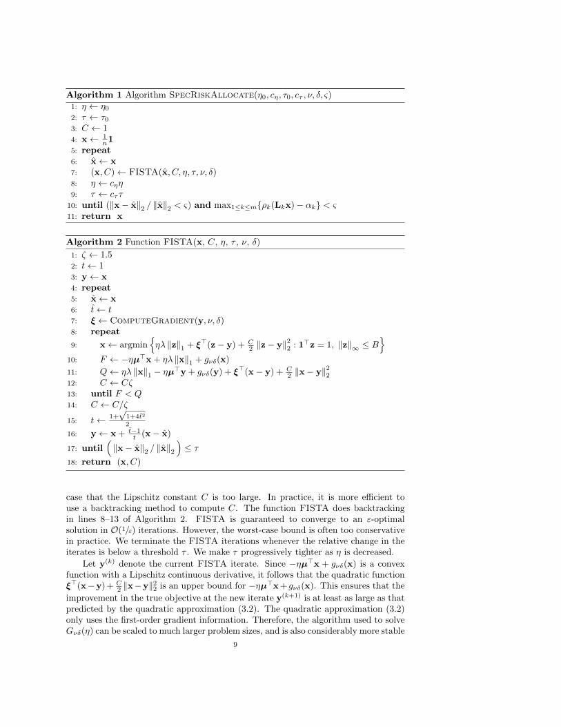
3.2. First-order proximal gradient algorithm. SpecRiskAllocate is dis-played in Algorithm 1. SpecRiskAllocate computes an ε-optimal solution for thespectral risk constrained portfolio selection problem (2.2) by approximately solvinga sequence of smoothed penalty problems Gνδ(η) for a decreasing sequence of η. Webegin with η ← η0 and then progressively reduce η ← cηη, where cη < 1. This contin-uation scheme ensures that SpecRiskAllocate is able to take large steps when theiterates are far from optimality. In Theorem 3.1 we showed that there exists η∗ > 0such that we can recover an ε-optimal solution for (2.2) by solving Gνδ(η

∗), i.e. wedo not have to drive η all the way to zero. This feature adds stability to SpecRisk-Allocate since the numerical accuracy required to solve Gνδ(η) increases as η 0(see e.g. Nocedal and Wright [1999]). In practice, we stop whenever the relativechange in iterate x(j) is smaller than the tolerance ς, and the iterate x(j) is ς-feasible,i.e. gmax(x(j)) ≤ ς. SpecRiskAllocate calls FISTA to approximately solve Gνδ(η)for a fixed value of η. FISTA is a proximal gradient method, i.e. a gradient descentalgorithm with an additional proximal term to control the step length. The parame-ter τ controls the accuracy demanded by FISTA. We need τ 0 to ensure that theaccuracy is increased as η 0.

Next we describe some of the essential features of FISTA. We refer the readerto Beck and Teboulle [2009] for the details of the algorithm. The particular imple-mentation of FISTA that we employ is displayed in Algorithm 2. FISTA computesan approximate solution to Gνδ(η) by iteratively solving a sequence of quadratic op-timization problems of the form

(3.2)min ηλ ‖x‖1 + ξ>(x− y) + C

2 ‖x− y‖22 ,s.t. 1>x = 1,

‖x‖∞ ≤ B,

where ξ = ∇(−ηµ>y + gνδ(y)

)= −ηµ +∇gνδ(y), and C is the Lipschitz constant

of the gradient ξ. Although one can explicitly compute its value, it is often the

8

Algorithm 1 Algorithm SpecRiskAllocate(η0, cη, τ0, cτ , ν, δ, ς)1: η ← η0

2: τ ← τ03: C ← 14: x← 1

n15: repeat6: x← x7: (x, C)← FISTA(x, C, η, τ, ν, δ)8: η ← cηη9: τ ← cττ

10: until (‖x− x‖2 / ‖x‖2 < ς) and max1≤k≤mρk(Lkx)− αk < ς11: return x

Algorithm 2 Function FISTA(x, C, η, τ , ν, δ)

1: ζ ← 1.52: t← 13: y← x4: repeat5: x← x6: t← t7: ξ ← ComputeGradient(y, ν, δ)8: repeat

9: x← argminηλ ‖z‖1 + ξ>(z− y) + C

2 ‖z− y‖22 : 1>z = 1, ‖z‖∞ ≤ B

10: F ← −ηµ>x + ηλ ‖x‖1 + gνδ(x)

11: Q← ηλ ‖x‖1 − ηµ>y + gνδ(y) + ξ>(x− y) + C2 ‖x− y‖22

12: C ← Cζ13: until F < Q14: C ← C/ζ

15: t← 1+√

1+4t2

2

16: y← x + t−1t (x− x)

17: until(‖x− x‖2 / ‖x‖2

)≤ τ

18: return (x, C)

case that the Lipschitz constant C is too large. In practice, it is more efficient touse a backtracking method to compute C. The function FISTA does backtrackingin lines 8–13 of Algorithm 2. FISTA is guaranteed to converge to an ε-optimalsolution in O(1/ε) iterations. However, the worst-case bound is often too conservativein practice. We terminate the FISTA iterations whenever the relative change in theiterates is below a threshold τ . We make τ progressively tighter as η is decreased.

Let y(k) denote the current FISTA iterate. Since −ηµ>x + gνδ(x) is a convexfunction with a Lipschitz continuous derivative, it follows that the quadratic functionξ>(x−y) + C

2 ‖x−y‖22 is an upper bound for −ηµ>x + gνδ(x). This ensures that the

improvement in the true objective at the new iterate y(k+1) is at least as large as thatpredicted by the quadratic approximation (3.2). The quadratic approximation (3.2)only uses the first-order gradient information. Therefore, the algorithm used to solveGνδ(η) can be scaled to much larger problem sizes, and is also considerably more stable

9

as the problem size increases, as compared to a full-fledged quadratic approximationthat uses all the Hessian information; however, at the cost of a larger iteration count.Finally, note that (3.2) is equivalent to

min ηλ ‖x‖1 + (ξ − Cy)>x + C2 x>x,

s.t. 1>x = 1,‖x‖∞ ≤ B,

i.e. the FISTA iterates are computed by solving an `1-penalized separable convexQP with the number of decision variables equal to the number of assets. Thus, thisproblem can be solved very efficiently if one has access to a mean-variance solver.In Appendix B we show how to solve this problem using a single one-dimensionalsearch. In practical instances, where it is likely that the portfolio selection problemhas additional linear constraints, the portfolio manager can use the mean-variance orquadratic solver to compute the FISTA iterates. In Appendix B, we also show howto compute the gradient ξ using

∑mk=1 dk + 1 one-dimensional searches.

4. Numerical results. In this section we present numerical experiments thatshow the advantage of SpecRiskAllocate over the LP formulation when dealingwith large instances of the spectral risk constrained portfolio selection problem. Next,we illustrate the convenience of considering several risk models to overcome the un-certainty in risk parameters when selecting a portfolio to hedge the risk of an existingone.

4.1. Ill-Conditioning and Problem Scaling Results. We tested our algo-rithm on random instances of the spectral risk constrained portfolio selection prob-lem (2.2). We generated instances with different values for the number of assets n.The number of spectral risk constraints was m = 5 for all instances. For each spectralrisk measure, we fixed the number of ES components to d = 3. The number of lossscenarios N was set equal for all risk models. We randomly generated the expectedreturn percentage vector µ, the scenario-based loss matrices Lk, the ES weight vec-tors γk, and the ES levels βk ∈ [0.9, 1)d. The spectral risk budgets αk were set toαk−0.1 |αk|, where αk is the value of the k-th spectral risk measure ρk(Lkx) at port-folio x = 1/n1. We set the leverage bound to B = 1, and the parameter controllingthe sparsity of the portfolio either to λ = 0 or λ = λ∗, where λ∗ = 2

∣∣∣µ>x∗∣∣∣/‖x∗‖1, and

x∗ = argmaxµ>x : 1>x = 1, ‖x‖∞ ≤ B. For all the instances generated, the valueof λ∗ was in the interval [0.01, 0.03]. The SpecRiskAllocate parameters were setas follows

η0 = 10, cη = 0.99, τ0 = 10−4, cτ = 0.95, ν = 0.01 min |αk|, δ = 0.01, ς = 10−2.

We solved each instance of the spectral risk constrained sparse portfolio selection prob-lem using a MATLAB implementation of SpecRiskAllocate. For each instance, wealso solved the LP formulation (2.3) using the state-of-the-art LP solver Gurobi [GurobiOptimization, Inc., 2014] with an optimality tolerance of ς = 10−2. We solved theinstances using Gurobi version 5.0.2 and Gurobi version 5.6.0. Our results indicatethat, although the performance of Gurobi has improved significantly from one versionto the other, our algorithm still offers a significant advantage over this state-of-the-art LP solver. We called Gurobi from MATLAB using Gurobi’s MATLAB interface.MATLAB was run on a 6-core, 3.07GHz Intel Xeon processor with 66GB of RAMrunning the Ubuntu OS.

10

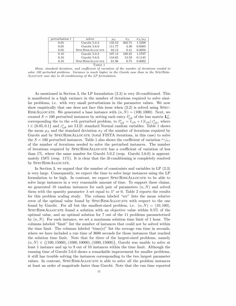
perturbation t solver µS σS σS/µS0.05 Gurobi 5.0.2 132.53 202.75 1.52980.05 Gurobi 5.6.0 111.77 4.30 0.03850.05 SpecRiskAllocate 82.12 0.41 0.00500.10 Gurobi 5.0.2 107.14 169.25 1.57970.10 Gurobi 5.6.0 118.65 13.59 0.11450.10 SpecRiskAllocate 81.96 0.75 0.0092

Table 1Mean, standard deviation, and coefficient of variation of the number of iterations needed to

solve 100 perturbed problems. Variance is much higher in the Gurobi case than in the SpecRisk-Allocate case due to ill-conditioning of the LP formulation.

As mentioned in Section 3, the LP formulation (2.3) is very ill-conditioned. Thisis manifested in a high variance in the number of iterations required to solve simi-lar problems, i.e. with very small perturbations in the parameter values. We nowshow empirically that one does not face this issue when (2.2) is solved using Spec-RiskAllocate. We generated a base instance with (n,N) = (100, 1000). Next, wecreated S = 100 perturbed instances by setting each entry `sijk of the loss matrix Lsk,corresponding the to the s-th perturbed problem, to `sijk = `ijk + t |`ijk| εsijk, wheret ∈ 0.05, 0.1 and εsijk are I.I.D. standard Normal random variables. Table 1 showsthe mean µS and the standard deviation σS of the number of iterations required byGurobi and by SpecRiskAllocate (total FISTA iterations, in this case) to solvethe S = 100 perturbed instances. Table 1 also shows the coefficient of variation σS/µS

of the number of iterations needed to solve the perturbed instances. The numberof iterations required by SpecRiskAllocate has a coefficient of variation of lessthan 1%, where the same number for Gurobi 5.0.2 (resp. Gurobi 5.6.0) is approxi-mately 158% (resp. 11%). It is clear that the ill-conditioning is completely resolvedby SpecRiskAllocate.

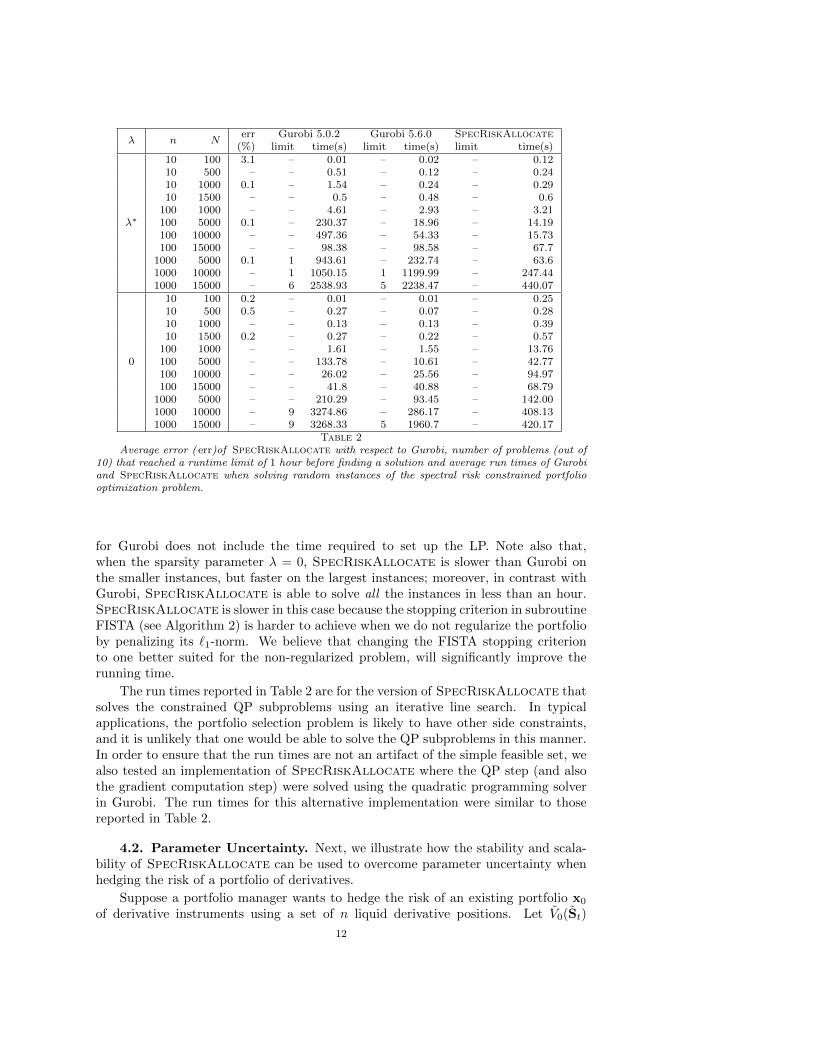
In Section 3, we argued that the number of constraints and variables in LP (2.3)is very large. Consequently, we expect the time to solve large instances using the LPformulation to be high. In contrast, we expect SpecRiskAllocate to be able tosolve large instances in a very reasonable amount of time. To support these claims,we generated 10 random instances for each pair of parameters (n,N) and solvedthem with the sparsity parameter λ set equal to λ∗ or 0. Table 2 reports the resultsfor this problem scaling study. The column labeled “err” lists the mean relativeerror of the optimal value found by SpecRiskAllocate with respect to the onefound by Gurobi. For all but the smallest-sized problem, i.e. (n,N) = (10, 100),SpecRiskAllocate found a solution with an objective value within 0.5% of theoptimal value, and an optimal solution for 7 out of the 11 problems parameterizedby (n,N). For each instance, we set a maximum solution time limit of 1 hour. Thecolumns labeled “limit” list the number of instances that could not be solved withinthe time limit. The columns labeled “time(s)” list the average run time in seconds,where we have included a run time of 3600 seconds for those instances that reachedthe solution time limit. Note that for three of the largest-sized problems, namely(n,N) ∈ (100, 15000), (1000, 10000), (1000, 15000), Gurobi was unable to solve atleast 1 instance and up to 9 out of 10 instances within the time limit. Although therunning time of Gurobi 5.6.0 shows a remarkable improvement for smaller problems,it still has trouble solving the instances corresponding to the two largest parametervalues. In contrast, SpecRiskAllocate is able to solve all the problem instancesat least an order of magnitude faster than Gurobi. Note that the run time reported

11

λ n Nerr Gurobi 5.0.2 Gurobi 5.6.0 SpecRiskAllocate

(%) limit time(s) limit time(s) limit time(s)

λ∗

10 100 3.1 – 0.01 – 0.02 – 0.1210 500 – – 0.51 – 0.12 – 0.2410 1000 0.1 – 1.54 – 0.24 – 0.2910 1500 – – 0.5 – 0.48 – 0.6

100 1000 – – 4.61 – 2.93 – 3.21100 5000 0.1 – 230.37 – 18.96 – 14.19100 10000 – – 497.36 – 54.33 – 15.73100 15000 – – 98.38 – 98.58 – 67.7

1000 5000 0.1 1 943.61 – 232.74 – 63.61000 10000 – 1 1050.15 1 1199.99 – 247.441000 15000 – 6 2538.93 5 2238.47 – 440.07

0

10 100 0.2 – 0.01 – 0.01 – 0.2510 500 0.5 – 0.27 – 0.07 – 0.2810 1000 – – 0.13 – 0.13 – 0.3910 1500 0.2 – 0.27 – 0.22 – 0.57

100 1000 – – 1.61 – 1.55 – 13.76100 5000 – – 133.78 – 10.61 – 42.77100 10000 – – 26.02 – 25.56 – 94.97100 15000 – – 41.8 – 40.88 – 68.79

1000 5000 – – 210.29 – 93.45 – 142.001000 10000 – 9 3274.86 – 286.17 – 408.131000 15000 – 9 3268.33 5 1960.7 – 420.17

Table 2Average error ( err)of SpecRiskAllocate with respect to Gurobi, number of problems (out of

10) that reached a runtime limit of 1 hour before finding a solution and average run times of Gurobiand SpecRiskAllocate when solving random instances of the spectral risk constrained portfoliooptimization problem.

for Gurobi does not include the time required to set up the LP. Note also that,when the sparsity parameter λ = 0, SpecRiskAllocate is slower than Gurobi onthe smaller instances, but faster on the largest instances; moreover, in contrast withGurobi, SpecRiskAllocate is able to solve all the instances in less than an hour.SpecRiskAllocate is slower in this case because the stopping criterion in subroutineFISTA (see Algorithm 2) is harder to achieve when we do not regularize the portfolioby penalizing its `1-norm. We believe that changing the FISTA stopping criterionto one better suited for the non-regularized problem, will significantly improve therunning time.

The run times reported in Table 2 are for the version of SpecRiskAllocate thatsolves the constrained QP subproblems using an iterative line search. In typicalapplications, the portfolio selection problem is likely to have other side constraints,and it is unlikely that one would be able to solve the QP subproblems in this manner.In order to ensure that the run times are not an artifact of the simple feasible set, wealso tested an implementation of SpecRiskAllocate where the QP step (and alsothe gradient computation step) were solved using the quadratic programming solverin Gurobi. The run times for this alternative implementation were similar to thosereported in Table 2.

4.2. Parameter Uncertainty. Next, we illustrate how the stability and scala-bility of SpecRiskAllocate can be used to overcome parameter uncertainty whenhedging the risk of a portfolio of derivatives.

Suppose a portfolio manager wants to hedge the risk of an existing portfolio x0

of derivative instruments using a set of n liquid derivative positions. Let V0(St)

12

and Vi(St) denote, respectively, the value of the initial portfolio x0 and the value ofderivative instrument i ∈ 1, . . . , n at time t, as functions of the vector of underlyingasset prices St ∈ Rs. Let ˜

0(t) = V0(S0) − V0(St) (resp. ˜i(t) = Vi(S0) − Vi(St))

denote the loss of the initial portfolio (resp. derivative instrument i) at time t. Then,the loss at time t of a hedging portfolio x ∈ Rn is given by

∑ni=1

˜i(t)xi, and the total

loss at time t for the portfolio manager is ˜0(t) +

∑ni=1

˜i(t)xi. Note that, in contrast

with our previous notation, xi now denotes the total number of units of derivative ipurchased. Therefore, in what follows we drop the portfolio constraint 1>x = 1.

Suppose the underlying asset prices St are log-normally distributed with meanvector π and unknown covariance matrix Σt = DtRDt, where R is a constant cor-relation matrix and Dt = diag(σt) is a diagonal matrix of unknown volatilities attime t. Suppose the portfolio manager knows the current volatility σ0, and believesthat the volatility at the time horizon T is of the form σT = σ0 +

∑qp=1 ωpρp, where

ρp ∈ Rs are known factors and ωp ∈ [−1, 1] are the corresponding unknown weights.

For ω ∈ Ω := −1, 1q ∪ 0, let `0(ω) ∈ RN (resp `i(ω) ∈ RN ) denote the vector ofN samples of the loss ˜

0(T ) on the initial portfolio (resp. the loss ˜i(T ) on derivative

instrument i) when the volatility vector σT = σ0 +∑qp=1 ωpρp. For a subset W of

Ω, consider the following hedging portfolio selection problem:

Π(W ) : = maxx

minω∈Wµ0 + µ(ω)>x− λ ‖x‖1

s.t. ESβ(`0(ω) + L(ω)x) ≤ αESβ(`0(ω)), ω ∈W

‖x‖∞ ≤ B

(4.1)

= maxx,µ

µ− λ ‖x‖1s.t. µ ≤ µ0 + µ(ω)>x, ω ∈W

ESβ(`0(ω) + L(ω)x) ≤ αESβ(`0(ω)), ω ∈W‖x‖∞ ≤ B,

where L(ω) = [`1(ω) . . . `n(ω)], µ(ω) = − 1NL(ω)>1, and µ0 = − 1

N `0(ω)>1. Bysolving problem (4.1), the portfolio manager is looking to compute an `1-regularizedhedging portfolio x that maximizes the worst-case (w.r.t. W ) expected return ofthe total portfolio [x>0 ,x

>]>, while ensuring that the worst case expected shortfalldrops by factor of α < 1. We define Π(0) (resp. Π(−1, 1q)) as the nominal(resp. robust) portfolio selection problem. Since we allow the hedging portfolio x tohave both long and short positions, in order to be robust against uncertainty in theparameters ωp we must consider all the possible worst-case risk models ω ∈ −1, 1q.Problem (4.1) is equivalent to

maxx

µ>x− λ ‖x‖1s.t. ES0(`0(ω) + L(ω)x) ≤ 0, ω ∈W

ESβ(`0(ω) + L(ω)x) ≤ αESβ(`0(ω)), ω ∈Wl ≤ x ≤ u,

(4.2)

where x = [x>, µ+, µ−]>, µ = [0>, λ + 1, λ − 1]>, L(ω) = [L(ω),1,−1], L(ω) =[L(ω),0,0], l = [−B1>, 0, 0]>, and u = [B1>,∞,∞]>. Thus, by slightly modifyingSpecRiskAllocate to deal with box constraints of the form l ≤ x ≤ u instead ofthe portfolio and leverage constraints 1>x = 1 and ‖x‖∞ ≤ B, we are able to exploitits stability and scalability to construct hedging portfolios that are robust againstparameter uncertainty.

In what follows, we show that, using SpecRiskAllocate, one can construct aportfolio that reduces the risk of the initial portfolio while removing the impact of

13

the uncertain parameters on the expected return. Following Alexander et al. [2003],we assumed that the initial portfolio consisted of four short positions of Europeanat-the-money binary call options, each on one of four correlated assets, with matu-rity in 4, 6, 8, and 10 months, respectively. The hedging universe was composed of20 vanilla European calls on each asset, given by the combination of strike prices[0.9, 0.95, 1, 1.05, 1.1]S0 and maturities [2, 3, 4, 6] months, and the assets themselves.The time horizon was T = 1 month. We used N = 25, 000 Monte Carlo samples tosimulate the underlying asset prices. The derivatives were priced using Black-Scholesformulae. The rest of the problem parameters were set as follows: the q = 2 factors af-fecting the volatility, ρ1 = 0.02[1, 1, 1, 1]> and ρ2 = 0.02[1,−1, 1,−1]>; the expectedshortfall level β = 0.95; the risk reduction factor α = 0.5, i.e. the portfolio manageris looking reduce his exposure by half; the leverage bound B = 1; and the parameter

controlling the sparsity of the portfolio λ = θ 2µ(0)>x∗

‖x∗‖1, where θ ∈ 0, 0.5, 1, and x∗

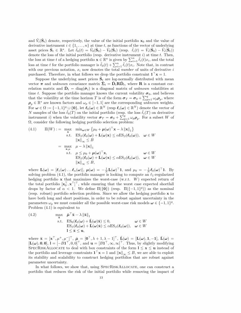
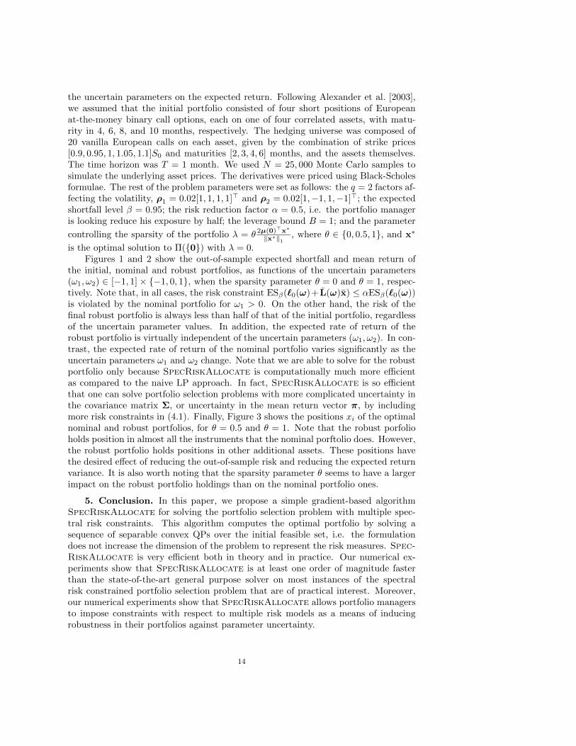
is the optimal solution to Π(0) with λ = 0.Figures 1 and 2 show the out-of-sample expected shortfall and mean return of

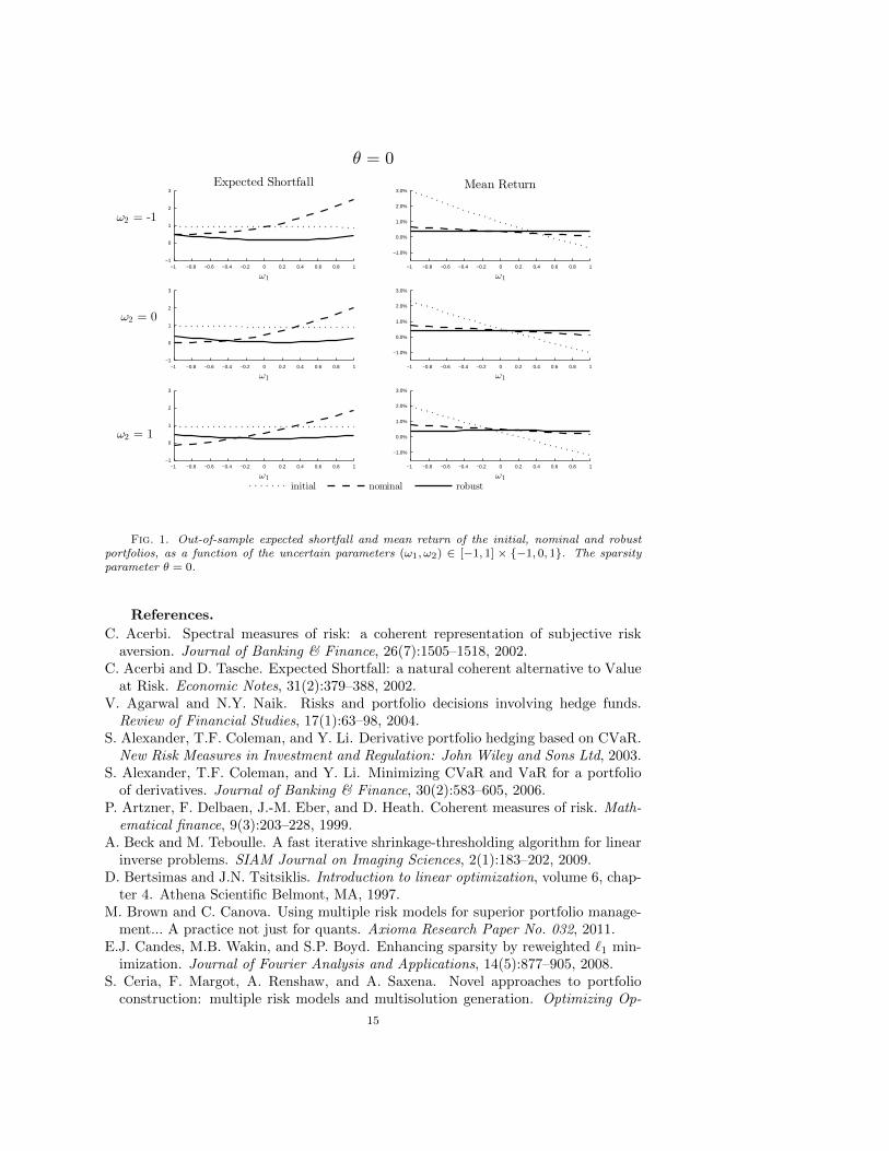
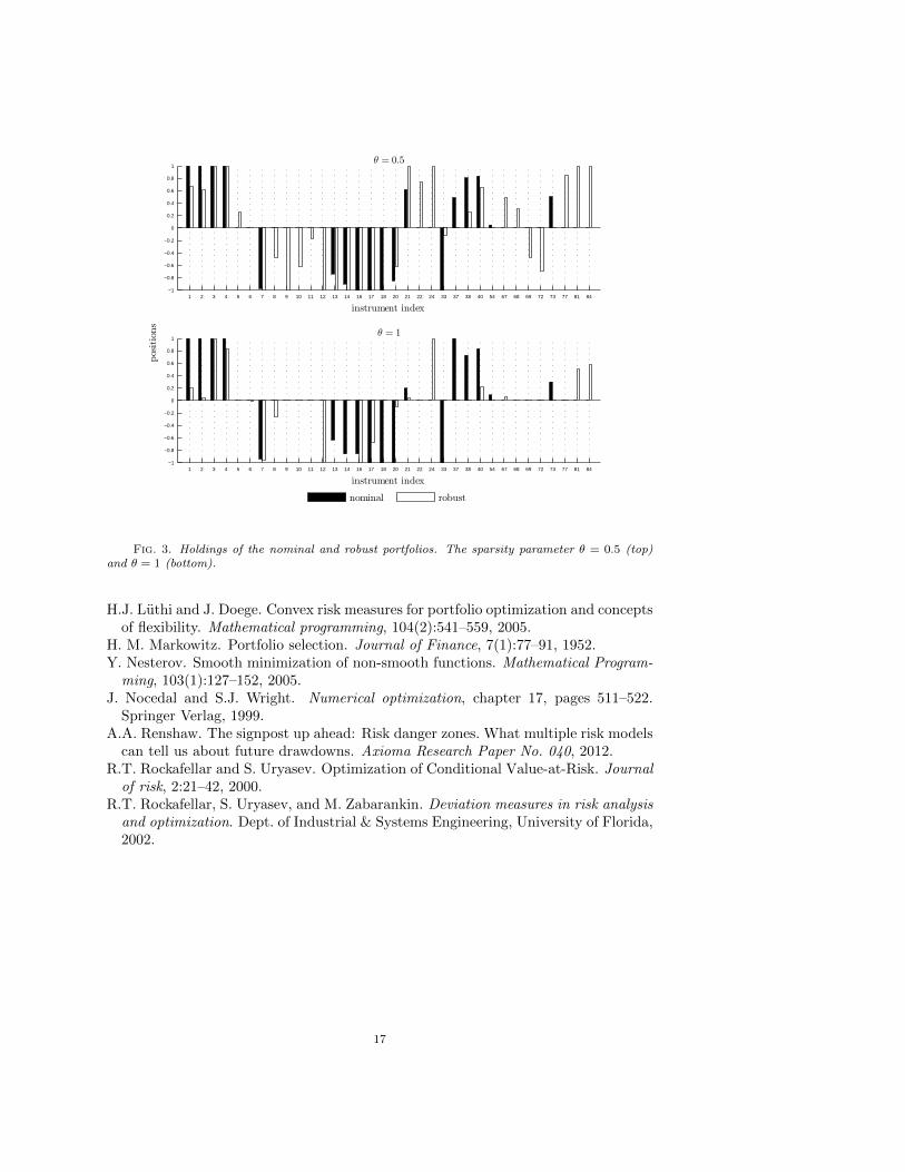
the initial, nominal and robust portfolios, as functions of the uncertain parameters(ω1, ω2) ∈ [−1, 1]× −1, 0, 1, when the sparsity parameter θ = 0 and θ = 1, respec-tively. Note that, in all cases, the risk constraint ESβ(`0(ω)+ L(ω)x) ≤ αESβ(`0(ω))is violated by the nominal portfolio for ω1 > 0. On the other hand, the risk of thefinal robust portfolio is always less than half of that of the initial portfolio, regardlessof the uncertain parameter values. In addition, the expected rate of return of therobust portfolio is virtually independent of the uncertain parameters (ω1, ω2). In con-trast, the expected rate of return of the nominal portfolio varies significantly as theuncertain parameters ω1 and ω2 change. Note that we are able to solve for the robustportfolio only because SpecRiskAllocate is computationally much more efficientas compared to the naive LP approach. In fact, SpecRiskAllocate is so efficientthat one can solve portfolio selection problems with more complicated uncertainty inthe covariance matrix Σ, or uncertainty in the mean return vector π, by includingmore risk constraints in (4.1). Finally, Figure 3 shows the positions xi of the optimalnominal and robust portfolios, for θ = 0.5 and θ = 1. Note that the robust porfolioholds position in almost all the instruments that the nominal porftolio does. However,the robust portfolio holds positions in other additional assets. These positions havethe desired effect of reducing the out-of-sample risk and reducing the expected returnvariance. It is also worth noting that the sparsity parameter θ seems to have a largerimpact on the robust portfolio holdings than on the nominal portfolio ones.

5. Conclusion. In this paper, we propose a simple gradient-based algorithmSpecRiskAllocate for solving the portfolio selection problem with multiple spec-tral risk constraints. This algorithm computes the optimal portfolio by solving asequence of separable convex QPs over the initial feasible set, i.e. the formulationdoes not increase the dimension of the problem to represent the risk measures. Spec-RiskAllocate is very efficient both in theory and in practice. Our numerical ex-periments show that SpecRiskAllocate is at least one order of magnitude fasterthan the state-of-the-art general purpose solver on most instances of the spectralrisk constrained portfolio selection problem that are of practical interest. Moreover,our numerical experiments show that SpecRiskAllocate allows portfolio managersto impose constraints with respect to multiple risk models as a means of inducingrobustness in their portfolios against parameter uncertainty.

14

−1 −0.8 −0.6 −0.4 −0.2 0 0.2 0.4 0.6 0.8 1−1

0

1

2

3

ω1

ω2 = -1

Expected Shortfall

−1 −0.8 −0.6 −0.4 −0.2 0 0.2 0.4 0.6 0.8 1

−1.0%

0.0%

1.0%

2.0%

3.0%

ω1

Mean Return

−1 −0.8 −0.6 −0.4 −0.2 0 0.2 0.4 0.6 0.8 1−1

0

1

2

3

ω1

ω2 = 0

−1 −0.8 −0.6 −0.4 −0.2 0 0.2 0.4 0.6 0.8 1

−1.0%

0.0%

1.0%

2.0%

3.0%

ω1

−1 −0.8 −0.6 −0.4 −0.2 0 0.2 0.4 0.6 0.8 1−1

0

1

2

3

ω1

ω2 = 1

θ = 0

−1 −0.8 −0.6 −0.4 −0.2 0 0.2 0.4 0.6 0.8 1

−1.0%

0.0%

1.0%

2.0%

3.0%

ω1

initial nominal robust

Fig. 1. Out-of-sample expected shortfall and mean return of the initial, nominal and robustportfolios, as a function of the uncertain parameters (ω1, ω2) ∈ [−1, 1] × −1, 0, 1. The sparsityparameter θ = 0.

References.

C. Acerbi. Spectral measures of risk: a coherent representation of subjective riskaversion. Journal of Banking & Finance, 26(7):1505–1518, 2002.

C. Acerbi and D. Tasche. Expected Shortfall: a natural coherent alternative to Valueat Risk. Economic Notes, 31(2):379–388, 2002.

V. Agarwal and N.Y. Naik. Risks and portfolio decisions involving hedge funds.Review of Financial Studies, 17(1):63–98, 2004.

S. Alexander, T.F. Coleman, and Y. Li. Derivative portfolio hedging based on CVaR.New Risk Measures in Investment and Regulation: John Wiley and Sons Ltd, 2003.

S. Alexander, T.F. Coleman, and Y. Li. Minimizing CVaR and VaR for a portfolioof derivatives. Journal of Banking & Finance, 30(2):583–605, 2006.

P. Artzner, F. Delbaen, J.-M. Eber, and D. Heath. Coherent measures of risk. Math-ematical finance, 9(3):203–228, 1999.

A. Beck and M. Teboulle. A fast iterative shrinkage-thresholding algorithm for linearinverse problems. SIAM Journal on Imaging Sciences, 2(1):183–202, 2009.

D. Bertsimas and J.N. Tsitsiklis. Introduction to linear optimization, volume 6, chap-ter 4. Athena Scientific Belmont, MA, 1997.

M. Brown and C. Canova. Using multiple risk models for superior portfolio manage-ment... A practice not just for quants. Axioma Research Paper No. 032, 2011.

E.J. Candes, M.B. Wakin, and S.P. Boyd. Enhancing sparsity by reweighted `1 min-imization. Journal of Fourier Analysis and Applications, 14(5):877–905, 2008.

S. Ceria, F. Margot, A. Renshaw, and A. Saxena. Novel approaches to portfolioconstruction: multiple risk models and multisolution generation. Optimizing Op-

15

−1 −0.8 −0.6 −0.4 −0.2 0 0.2 0.4 0.6 0.8 1−1

0

1

2

3

ω1

ω2 = -1

Expected Shortfall

−1 −0.8 −0.6 −0.4 −0.2 0 0.2 0.4 0.6 0.8 1

−1.0%

0.0%

1.0%

2.0%

3.0%

ω1

Mean Return

−1 −0.8 −0.6 −0.4 −0.2 0 0.2 0.4 0.6 0.8 1−1

0

1

2

3

ω1

ω2 = 0

−1 −0.8 −0.6 −0.4 −0.2 0 0.2 0.4 0.6 0.8 1

−1.0%

0.0%

1.0%

2.0%

3.0%

ω1

−1 −0.8 −0.6 −0.4 −0.2 0 0.2 0.4 0.6 0.8 1−1

0

1

2

3

ω1

ω2 = 1

θ = 1

−1 −0.8 −0.6 −0.4 −0.2 0 0.2 0.4 0.6 0.8 1

−1.0%

0.0%

1.0%

2.0%

3.0%

ω1

initial nominal robust

Fig. 2. Out-of-sample expected shortfall and mean return of the initial, nominal and robustportfolios, as a function of the uncertain parameters (ω1, ω2) ∈ [−1, 1] × −1, 0, 1. The sparsityparameter θ = 1.

timization: The Next Generation of Optimization Applications & Theory, pages23–52, 2009.

T.J. Chang, N. Meade, JE Beasley, and YM Sharaiha. Heuristics for cardinalityconstrained portfolio optimisation. Computers and Operations Research, 27(13):1271–1302, 2000.

V. DeMiguel, L. Garlappi, F.J. Nogales, and R. Uppal. A generalized approach toportfolio optimization: Improving performance by constraining portfolio norms.Management Science, 55(5):798–812, 2009.

Gurobi Optimization, Inc. Gurobi optimizer reference manual, 2014. URL http:

//www.gurobi.com.S. Hoda, A. Gilpin, J. Pena, and T. Sandholm. Smoothing techniques for computing

Nash equilibria of sequential games. Mathematics of Operations Research, 35(2):494–512, 2010.

G. Iyengar and A.K.C. Ma. Fast gradient descent method for mean-CVaR optimiza-tion. Annals of Operations Research, 205(1):203–212, 2013.

G. Iyengar, D.J. Phillips, and C. Stein. Approximating semidefinite packing programs.SIAM Journal on Optimization, 21(1):231–268, 2011.

P. Jorion. Value at Risk. McGraw-Hill, New York, 2006.Y.A. Koskosidis and A.M. Duarte. A scenario-based approach to active asset alloca-

tion. The Journal of Portfolio Management, 23(2):74–85, 1997.A.E.B. Lim, J.G. Shanthikumar, and G.-Y. Vahn. Conditional Value-at-Risk in port-

folio optimization: Coherent but fragile. Operations Research Letters, 39(3):163–171, 2011.

16

1 2 3 4 5 6 7 8 9 10 11 12 13 14 16 17 18 20 21 22 24 33 37 38 40 54 67 68 69 72 73 77 81 84−1

−0.8

−0.6

−0.4

−0.2

0

0.2

0.4

0.6

0.8

1

instrument index

θ = 0.5

1 2 3 4 5 6 7 8 9 10 11 12 13 14 16 17 18 20 21 22 24 33 37 38 40 54 67 68 69 72 73 77 81 84−1

−0.8

−0.6

−0.4

−0.2

0

0.2

0.4

0.6

0.8

1

instrument index

θ = 1

positions

nominal robust

Fig. 3. Holdings of the nominal and robust portfolios. The sparsity parameter θ = 0.5 (top)and θ = 1 (bottom).

H.J. Luthi and J. Doege. Convex risk measures for portfolio optimization and conceptsof flexibility. Mathematical programming, 104(2):541–559, 2005.

H. M. Markowitz. Portfolio selection. Journal of Finance, 7(1):77–91, 1952.Y. Nesterov. Smooth minimization of non-smooth functions. Mathematical Program-

ming, 103(1):127–152, 2005.J. Nocedal and S.J. Wright. Numerical optimization, chapter 17, pages 511–522.

Springer Verlag, 1999.A.A. Renshaw. The signpost up ahead: Risk danger zones. What multiple risk models

can tell us about future drawdowns. Axioma Research Paper No. 040, 2012.R.T. Rockafellar and S. Uryasev. Optimization of Conditional Value-at-Risk. Journal

of risk, 2:21–42, 2000.R.T. Rockafellar, S. Uryasev, and M. Zabarankin. Deviation measures in risk analysis

and optimization. Dept. of Industrial & Systems Engineering, University of Florida,2002.

17

Appendix A. Smoothing of g(x). Define the function

(A.1) f(ν)β (ζ) = max ζ>q− ν

2 ‖q‖2s.t. 0 ≤ q ≤ 1

(1−β)N 1,

1>q = 1.

Nesterov [2005] establishes that f(ν)β (ζ) is a differentiable strongly convex function

with gradient ∇f (ν)β (ζ) = q∗, where q∗ is the unique solution to (A.1). The gradient

∇f (ν)β is Lipschitz continuous with Lipschitz constant 1/ν. Moreover, f

(ν)β satisfies

ESβ(ζ)− ν ≤ f (ν)β (ζ) ≤ ESβ(ζ), i.e. f

(ν)β (ζ) is a ν-approximation to ESβ(ζ).

Let ρ(ζ) =∑d`=1 γ`ESβ`

(ζ) denote any generalized spectral risk function. Wedefine the smoothed spectral risk function as

ρ(ν)(ζ) =

d∑`=1

γ`f(ν)β`

(ζ).

Since∑d`=1 γ` = 1 for all generalized spectral risk functions, it follows that ρ(ζ)−ν ≤

ρ(ν)(ζ) ≤ ρ(ζ). The gradient of ρ(ν)(ζ) is given by ∇ρ(ν)(ζ) =∑d`=1 γ`q

∗` , where q∗`

is the unique optimal solution to (A.1) with β = β`.

Finally, define

(A.2) Ψ(δ)(t) = max t>u− δ2 ‖u‖2

s.t. 1>u = 1u ≥ 0.

Ψ(δ) is a differentiable convex function with Lipschitz continuous gradient ∇Ψ(δ)(t) =u∗, where u∗ is the unique solution to (A.2), and Lipschitz constant 1/δ [Nesterov,2005]. In addition, we have that Ψ(t)− δ ≤ Ψ(δ)(t) ≤ Ψ(t).

We define the smoothing of g(x) as

gνδ(x) = Ψ(δ)(ρ

(ν)1 (L1x)− α1, . . . , ρ

(ν)m (Lmx)− αm, 0

).

Theorem [7] in Iyengar et al. [2011] (see, also Hoda et al. [2010]) guarantees thatgνδ(x) is a convex function with Lipschitz continuous gradient

(A.3) ∇gνδ(x) =

m∑k=1

u∗kL>k∇ρ

(ν)k (Lkx),

where

u∗ = argmax∑mk=1 uk

(ρ

(ν)k (Lkx)− αk

)− δ

2 ‖u‖2s.t. 1>u = 1

u ≥ 0.

Moreover, gνδ(x) is a (ν+δ)-approximation to g(x), i.e. g(x)−ν−δ ≤ gνδ(x) ≤ g(x).

Appendix B. Details of SpecRiskAllocate.

18

Recall that the FISTA iterates are computed by solving an `1-penalized QP of theform (3.2). Next, we show how to solve this problem using a one-dimensional search.Dualizing the constraint 1>x = 1, we obtain the following optimization problem:

L(γ) = min‖x‖∞≤B

ηλ ‖x‖1 + (ξ − Cy + γ1)>x +

C

2x>x

.

Writing x = w− v, where w,v ≥ 0, observe that

L(γ) = min0≤w≤B1

(ηλ1 + ξ − Cy + γ1)

>w +

C

2w>w

+ min

0≤v≤B1

(ηλ1− ξ + Cy− γ1)

>v− C

2v>v

,

where we have ignored the cross terms w>v because they are zero in any optimalsolution. The optimal solution to L(γ) is given by x∗i (γ) = min (ci − γ)/C,B+ −min (ci + γ)/C,B+, where ci = −ηλ−ξi+Cyi, and ci = −ηλ+ξi−Cyi, i = 1, . . . , n.The optimal solution to (3.2) can be recovered by finding the dual variable γ∗ such that1>x∗(γ∗) = 1. Since limγ→∞ x∗(γ) = −B1 and limγ→−∞ x∗(γ) = B1, it follows thatthere exists γ∗ ∈ (−∞,∞) such that 1>x∗(γ∗) = 1. The computational complexityof finding γ∗ is dominated by the computational cost of sorting the set ∪1≤i≤nci, ci.

FISTA (see Algorithm 2) calls subroutine ComputeGradient, displayed in Algo-rithm 3, to compute the gradient ξ. Computing gradient ξ requires computing thegradient ∇gνδ(x) (cf. (A.3)), which requires solving one QP of the form (A.2) and∑mk=1 dk QPs of the form (A.1). Each of these QPs is of the form

(B.1)max c>x− 1

2 ‖x‖22 ,

s.t. 1>x = 1,0 ≤ x ≤ b,

where the bound b ≥ 0 satisfies 1>b ≥ 1, and is possibly infinite. Dualizing theconstraint 1>x = 1, we obtain the following separable QP:

L(γ) = max0≤x≤b

n∑i=1

(ci − γ)xi −1

2x2i

.

The optimal solution to L(γ) is given by x∗i (γ) = minci − γ, bi+, i = 1, . . . , n.The optimal solution to (B.1) can be recovered by finding the dual variable γ∗ suchthat 1>x∗(γ∗) = 1. Since limγ→∞ x∗(γ) = 0 and limγ→−∞ x∗(γ) = b, it follows thatthere exists γ∗ ∈ (−∞,∞) such that 1>x∗(γ∗) = 1. The computational complexity ofcomputing γ∗ is dominated by the computational cost of sorting the set ∪1≤i≤nci, ci−bi.

19

Algorithm 3 Function ComputeGradient(y, ν, δ)

1: for k = 1 to m do2: for ` = 1 to dk do

3: qk` ← argmax

q>Lky− ν2 ‖q‖

22 : 1>q = 1, 0 ≤ q ≤ 1

(1−βk`)Nk1

4: end for5: end for6: u← argmax

∑mk=1 vk(ρ

(ν)k (Lky)− αk)− δ

2 ‖v‖22 :∑m+1k=1 vk = 1,v ≥ 0

7: ξ ← −ηµ+

∑mk=1 uk

(∑dk`=1 γk`L

>k qk`

)8: return ξ

20