Doppler Spectroscopy of an Ytterbium Bose-Einstein Condensate on the ClockTransition

A. Dareau, M. Scholl, Q. Beaufils, D. Doring,∗ J. Beugnon, and F. GerbierLaboratoire Kastler Brossel, College de France, CNRS, ENS-PSL Research University,

UPMC-Sorbonne Universites, 11 place Marcelin-Berthelot, 75005 Paris(Dated: August 29, 2018)

We describe Doppler spectroscopy of Bose-Einstein condensates of ytterbium atoms using a narrowoptical transition. We address the optical clock transition around 578 nm between the 1S0 and 3P0

states with a laser system locked on a high-finesse cavity. We show how the absolute frequency ofthe cavity modes can be determined within a few tens of kHz using high-resolution spectroscopyon molecular iodine. We show that optical spectra reflect the velocity distribution of expandingcondensates in free fall or after releasing them inside an optical waveguide. We demonstrate sub-kHz spectral linewidths, with long-term drifts of the resonance frequency well below 1 kHz/hour.These results open the way to high-resolution spectroscopy of many-body systems.

PACS numbers: 67.85.De,32.30.Jc,33.20.Kf,

I. INTRODUCTION

Since its early days, the field of ultracold atoms hastraditionally been focused on alkali atoms, which featurea strong, closed transition favorable for laser cooling andtrapping. In the last ten years, a lot of progress hasbeen made in bringing more complex atoms to quan-tum degeneracy [1–5]. Two-electron atoms, for instancefrom the alkaline-earth family or ytterbium, have beenof particular interest because of one special feature, anultranarrow J = 0 → J ′ = 0 optical transition fromthe 1S0 ground state to a metastable 3P0 optically ex-cited state (here J, J ′ denote the electronic angular mo-mentum for the ground and excited states). Althoughelectric dipole-forbidden, the transition can be weaklyenabled by hyperfine interactions or an applied magneticfield [6, 7]. Mastering the laser technology required toobserve such transitions with a spectroscopic resolutionat or below the Hertz level enabled the development ofoptical atomic clocks (see [8, 9] for reviews of this field,and [6, 7, 10–13] for specific realizations using ytterbiumatoms). Although optical atomic clocks are typically op-erated using dilute samples far from quantum degeneracy,many-body effects are nevertheless measurable becauseof the extreme spectroscopic sensitivity [14].

A number of proposals have been made to use such“clock” transitions, virtually free from spontaneous emis-sion, to manipulate quantum-degenerate gases, with di-verses purposes ranging from quantum information pro-cessing [15, 16] to the realization of effective magneticfields [17] or strongly-interacting impurity models [18]in optical lattices. In this article, we report on high-resolution spectroscopy on Bose-Einstein condensates(BECs) of ytterbium atoms, a first step towards morecomplex experiments using the clock transition. We use

∗Current address: FARO Scanner Production GmbH, Lingwiesen-strasse 11/2, D-70825 Korntal-Munchingen

here bosonic 174Yb and demonstrate how spectroscopicfeatures of the 1S0 → 3P0 transition, observed with sub-kHz resolution, can yield informations about the veloc-ity distribution. Previously, spectroscopy of trapped Ybcondensates on another ultranarrow J = 0 → J ′ = 2transition has been demonstrated [19–21]. This tran-sition is sensitive to magnetic fields. As a result, the1S0 → 3P0 transition is expected to offer a better spec-tral resolution, at the expense of a much weaker transi-tion strength. Spectroscopy of trapped Yb Fermi gases inthree-dimensional optical lattices was reported in [22, 23].

The article is organized as follows. In Section II, we de-scribe our experimental setup used to generate the laserlight probing the clock transition, including a high-finesseoptical cavity used for locking the laser frequency. InSection III, we show how we calibrate the absolute cav-ity frequency using an auxiliary spectroscopic referencebased on molecular iodine [24]. Section IV describes spec-troscopy on Yb BECs, where the condensate is first re-leased from the trap to reduce the interaction energy.The resulting spectra are dominated by the velocity dis-tribution of the expanding condensate, allowing us tomeasure spectra with widths of a few kHz. A single-shot technique to locate the laser frequency is presentedin Section IV C. Finally, we conclude in Section V.

II. EXPERIMENTAL SETUP

A. Optical setup

The main features of our experimental setup are shownin Figure 1. Narrow-linewidth laser light with wavelengthλL = 578.4 nm is generated by sum-frequency mixing oftwo infrared lasers in a non-linear crystal [24, 25]. Theinfrared laser sources used in this work are a solid-statelaser emitting around 200 mW near 1319 nm and an am-plified fiber laser emitting around 500 mW near 1030 nm.The frequency of both lasers is controlled using a piezo-electric transducer (PZT) on the laser cavities. The two

arX

iv:1

412.

5751

v1 [

cond

-mat

.qua

nt-g

as]

18

Dec

201

4

2

FIG. 1: Layout of the optical setup. A laser source at578.4 nm is sent to three different paths, one leading to anultrastable cavity to which the laser frequency is locked, oneleading to the trapped atomic sample, and one used for io-dine spectroscopy. The inset shows the spacing between the

various frequencies involved, with ω(n)cav the cavity mode to

which the laser frequency is locked and ωeg the clock tran-sition frequency. AOM: acoustic-optical modulator. EOM:electro-optical modulator. ULE: ultra-low expansion glass.SA: saturated absorption.

lasers are coupled into an optical waveguide made fromperiodically-poled Lithium Niobate. The output of thewaveguide is sent to a first acousto-optical modulator(AOM1), shifting the light frequency by a quantity δω1.This AOM is used to control the laser frequency to en-sure it remains resonant with the cavity, and to controlits intensity. The laser is then split among three paths, afirst one leading to an ultrastable optical cavity that weuse as a stable frequency reference (see Section II B), asecond one leading to the atoms via an optical fiber (seeSection IV), and a third one to an iodine spectroscopycell used to calibrate the absolute frequency of the cav-ity (see Section III B). As detailed in Figure 1, AOMsare used to control independently the frequencies of thelight in each path. The cavity path includes an addi-tional electro-optical modulator adding frequency side-bands near 1 GHz. Its purpose will be explained in thefollowing. Single-mode, polarization maintaining opti-cal fibers are used to transport the light from the opti-cal bench where it is generated to the cavity and to themain experiment where ytterbium atoms are probed. Wedenote by ω1 the light frequency after passing throughAOM1, by ωL the frequency of the light used to probethe atoms and by ω′L the frequency of the light sent tothe cavity.

B. Cavity design and characteristics

We use an ultrastable Fabry-Perot optical cavity asfrequency reference to stabilize the frequency of the laserused to perform spectroscopy on the clock transition.This type of cavities have been extensively studied inthe past few years, in connection with the recent develop-ments in optical atomic clocks [26–31]. The cavity we useis a commercial model from Advanced Thin Films (Boul-

der, Co), with a spherical body made from Ultra-lowexpansion (ULE) glass and two fused silica mirrors opti-cally contacted to the ULE glass. The cavity is held attwo points and placed inside a commercial housing (Sta-ble Laser Systems, Co) consisting of the cavity holdersurrounded by a gold-coated thermal shield, which areplaced inside a vacuum chamber. This isolates the cav-ity from detrimental pressure and temperature changes.The temperature of the thermal shield is actively stabi-lized to a few milliKelvins using a Peltier element and aservo control. Using an additional EOM (not shown inFigure 1), the laser frequency is locked to the cavity withthe Pound-Drever-Hall technique [32]. Frequency feed-back is applied by changing the frequency δω1 of AOM1,driven by a frequency synthesizer with fast modulationinput and wide modulation range (Agilent Technologiesmodel E4400B). An additional feedback path is used tocorrect for long term drifts by acting on the frequency-control input of the 1319 nm pump laser.

The cavity resonances are labeled by a longitudinal

mode index n, according to ω(n)cav = ω

(0)cav + n · ∆FSR,

where ∆FSR/2π = c/2L is the cavity free spectral range(FSR), L = 47.6(1) mm is the cavity length and c thespeed of light in vacuum. The free spectral range sep-arating two cavity resonances was calibrated using theEOM shown in Figure 1, which adds sidebands spacedby ∼ 1 GHz to the laser spectrum. We performed alinear scan of the laser frequency and recorded the fre-quencies for which the first positive sideband (frequencyω′L + δωEOM) is resonant with cavity mode n + 1 andthe second negative sideband (frequency ω′L − 2δωEOM)is resonant with cavity mode n. Taking the differencebetween the two measurements leads to the cavity FSR,∆FSR = 2π × 3 144 366(4) kHz (this measurement wasdone for a cavity temperature Tcav ≈ 5.0 C).

The width of each cavity resonance is determined bythe cavity finesse, dependent on the transmission of thecavity input coupler and other losses due to optical im-perfections, diffraction, etc ... The finesse is convenientlyobtained by measuring the cavity ring-down time byswitching off the incoming laser and monitoring the de-cay of the power transmitted through the cavity overtime. This measurement gives an exponential decaywith 1/e decay time constant τ ≈ 13 µs. Relating thistime constant to the cavity finesse F using the formulaτ−1 = ∆FSR/F , we find F ≈ 260 000, which is consistentwith the specifications of the manufacturer.

III. ABSOLUTE FREQUENCY CALIBRATIONOF THE CLOCK LASER USING

HIGH-RESOLUTION SPECTROSCOPY ONMOLECULAR IODINE

A. Motivation

When dealing with ultra-narrow lines, a key experi-mental issue is to be able to locate the resonance. For

3

iodine

spectroscopy (c)

−3 −2 −1 0 1 2 3δω1/2π (MHz)

cavity

tran

smiss

ion

∆ω2π

-100 -50 0 50 100ω/2π (kHz)

FIG. 2: (a): Frequency ruler showing the relative positions of several cavity resonances label with mode index n to n+ 3, theclock transition frequency labeled ωeg and the iodine resonance labeled ωI2 . (b): Close-up near the iodine resonance, showingthe relative positions of the different laser frequencies used for the spectroscopy when the iodine spectroscopy laser is resonant.(c): Experimental iodine absorption spectrum (top) and cavity transmission (bottom) as a function of laser frequency. Theinset shows a zoom on the narrow cavity resonance.

174Yb atoms and the 1S0 → 3P0 transition (hereafterdenoted ”clock transition”), accurate values of the tran-sition frequency have been measured by optical atomicclocks [6, 7, 11–13]. Measuring the laser frequency to thesame precision is however difficult, as the absolute cavityfrequency is a priori unknown. A basic method would beto perform first a coarse measurement of the cavity fre-quency (which can be done with a typical precision on theorder of hundred MHz using commercial wavemeters) andthen systematically search for the atomic resonance inthe interval corresponding to the frequency uncertainty.Needless to say, this is a cumbersome procedure, whichwould need to be done again each time the cavity reso-nance varies (intentionally or due to uncontrolled drifts).A more precise method to calibrate the cavity frequencyis clearly desirable. In principle, this is achievable withmodern technology combining frequency combs with sta-ble microwave atomic clocks [33].

When this technology is not available, an alternativeis to use an atomic or molecular line for frequency refer-ence. Fortunately, in the case of the 1S0 → 3P0 transi-tion in 174Yb, a nearby resonance in molecular iodinehas already been identified and characterized with anuncertainty of ∼2 kHz [24]. This molecular resonance,located approximately 10 GHz to the blue of the Ytter-bium clock transition, corresponds to one particular hy-perfine component of the so-called R(37)16-1 line. ThisΩ = 0→ Ω′ = 0 transition (Ω denotes the total molecu-lar angular momentum) is essentially unaffected by mag-netic fields and leads to narrow lines suitable to performaccurate frequency calibrations. In the following, we willdenote this specific transition (corresponding to a fre-quency ωI2) as “iodine transition” for simplicity. We alsolabel with “n” the cavity resonance closest to the clocktransition, and “n+3” the one closest to the iodine tran-sition located three FSRs away from the first one. Thescheme to measure the absolute laser frequency is then

clear : First, measure ∆ω = ωI2 − ω(n+3)cav , then deduce

ω(n)cav = ωI2−∆ω−3∆FSR using the value ωI2 measured in

[11] and the calibrated value for ∆FSR, and finally deducethe frequency ωL of the laser probing the atoms using theknown AOM frequencies (see Figure 2a).

B. Saturated absorption spectroscopy

To observe the iodine resonance, we perform saturatedabsorption (SA) spectroscopy on a quartz cell filled withmolecular iodine (lower path in Figure 1). We use a mod-ulation transfer spectroscopy scheme : The probe beamat frequency ω1 travels unmodulated through the cell,while the counter-propagating pump beam first passesthrough an additional AOM, shifting its frequency by+δωpump and modulating it for lock-in detection at thesame time. In such a geometry, the saturated absorptionresonance is reached when ωI2 = ω1 + δωpump/2. Theparticular line we investigate lies approximately 1.1 GHzaway to the red of the n + 3 cavity resonance (see Fig-ure 2b). We use the EOM in the cavity path to bridge thisfrequency gap, tuning its modulation frequency so thatthe first negative sideband on the cavity path is near then+ 3 cavity mode and the laser frequency is near the io-dine resonance. In this way, we are able to measure bothresonances within the same frequency scan. Typical SAand cavity transmission spectra are shown in Figure 2cwhen scanning the laser frequency. By fitting the data(absorption and transmission) to Lorentzians, we extractthe positions of the n + 3 cavity resonance and of theiodine resonance, which differ by a quantity ∆ω, the out-come of the measurement. The standard deviation of 10identical measurements performed with fixed parametersis below 10 kHz.

We have carefully looked for systematic effects thatcould affect this measurement. We have found no depen-dence on the power of the probe laser or applied magneticfield, but identified two effects that need to be accountedfor in the frequency measurement. A first effect is in-

4

strumental. The lock-in amplifier used to obtain the sat-urated absorption signal behaves as a first-order low passfilter with time constant 350 µs. This results in a slightshift of the center of the dispersive lock-in signal shownin Figure 2c from the iodine resonance. This is includedin our analysis, where the expected Lorentzian line shapeof the resonance is convoluted with the transfer functionof the lock-in and fitted to the measured signal to ex-tract the line position and width. The second correctionis due to collisions inside the iodine cell, which leads toline shift and broadening. We have carefully measuredthese effects and correct for them when evaluating themolecular resonance (see Appendix A).

Using this technique, we were able to quickly findthe Yb resonance by interrogating a sample of ultracoldatoms (see next Section). Repeating the measurementsallows us to track changes of the cavity resonance fre-quencies over time, either because of intended changesin the parameters (e.g. the temperature of the cavity),or because of uncontrolled environmental drifts. The er-ror in the absolute frequency is larger than the precisionof the measurement, and estimated to be a few tens ofkHz. When comparing a posteriori the laser frequencydeduced from the measured iodine resonance with respectto the actual one found from the atomic spectra, we ob-serve shifts of ≈ ±20 kHz which are stable to a few kHzover extended periods of time, but can vary with modifi-cations of the experimental setup. Possible explanationscould be errors in determining the collisional correction,or cell contamination [24]. According to the value givenin [7], the differential light shift due to the probe laseritself on the clock transition is around 1 kHz for our ex-perimental parameters, and therefore cannot explain theobserved difference between the observed resonance andthe one predicted from the cavity calibration.

C. Measurement of the zero-crossing of the cavityresonance with temperature

An important application of the spectroscopic calibra-tion technique described above is the determination ofthe zero-crossing point of the cavity. This refers to thechange of the resonance frequency with the cavity tem-

perature, dω(n+3)cav /dTcav, which quantifies the sensitivity

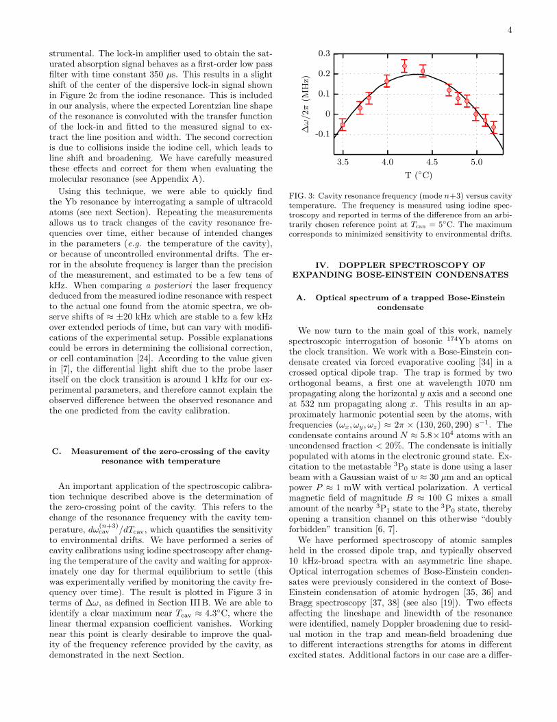
to environmental drifts. We have performed a series ofcavity calibrations using iodine spectroscopy after chang-ing the temperature of the cavity and waiting for approx-imately one day for thermal equilibrium to settle (thiswas experimentally verified by monitoring the cavity fre-quency over time). The result is plotted in Figure 3 interms of ∆ω, as defined in Section III B. We are able toidentify a clear maximum near Tcav ≈ 4.3C, where thelinear thermal expansion coefficient vanishes. Workingnear this point is clearly desirable to improve the qual-ity of the frequency reference provided by the cavity, asdemonstrated in the next Section.

3.5 4.0 4.5 5.0T (C)

-0.1

0

0.1

0.2

0.3

∆ω/2π

(MHz)

FIG. 3: Cavity resonance frequency (mode n+3) versus cavitytemperature. The frequency is measured using iodine spec-troscopy and reported in terms of the difference from an arbi-trarily chosen reference point at Tcan = 5C. The maximumcorresponds to minimized sensitivity to environmental drifts.

IV. DOPPLER SPECTROSCOPY OFEXPANDING BOSE-EINSTEIN CONDENSATES

A. Optical spectrum of a trapped Bose-Einsteincondensate

We now turn to the main goal of this work, namelyspectroscopic interrogation of bosonic 174Yb atoms onthe clock transition. We work with a Bose-Einstein con-densate created via forced evaporative cooling [34] in acrossed optical dipole trap. The trap is formed by twoorthogonal beams, a first one at wavelength 1070 nmpropagating along the horizontal y axis and a second oneat 532 nm propagating along x. This results in an ap-proximately harmonic potential seen by the atoms, withfrequencies (ωx, ωy, ωz) ≈ 2π × (130, 260, 290) s−1. Thecondensate contains around N ≈ 5.8×104 atoms with anuncondensed fraction < 20%. The condensate is initiallypopulated with atoms in the electronic ground state. Ex-citation to the metastable 3P0 state is done using a laserbeam with a Gaussian waist of w ≈ 30 µm and an opticalpower P ≈ 1 mW with vertical polarization. A verticalmagnetic field of magnitude B ≈ 100 G mixes a smallamount of the nearby 3P1 state to the 3P0 state, therebyopening a transition channel on this otherwise “doublyforbidden” transition [6, 7].

We have performed spectroscopy of atomic samplesheld in the crossed dipole trap, and typically observed10 kHz-broad spectra with an asymmetric line shape.Optical interrogation schemes of Bose-Einstein conden-sates were previously considered in the context of Bose-Einstein condensation of atomic hydrogen [35, 36] andBragg spectroscopy [37, 38] (see also [19]). Two effectsaffecting the lineshape and linewidth of the resonancewere identified, namely Doppler broadening due to resid-ual motion in the trap and mean-field broadening dueto different interactions strengths for atoms in differentexcited states. Additional factors in our case are a differ-

5

ential position-dependent light shift caused by the trappotential [19], and the collisional instability of the excitedstate. Inelastic collisions involving at least one excitedatom do not conserve the principal quantum number.Such collisions impart both collisional partners with a ki-netic energy much larger than the trap depth and resultin net atom losses at a rate γge = βgeng and γee = βeene,with ng (respectively ne) is the ground (resp. excited)state density. For 174Yb, the rate constants βge and βeeare not known, nor is the s−wave coupling constant ggedescribing g−e interactions (they have been measured forfermionic isotopes [39]). We note that the determinationof gge from the measured line shift suggested in [40] worksonly in absence of inelastic collisions and differential lightshifts. Rough estimates suggest that the mean field, po-tential energy and inelastic losses contribute each a fewkHz to the line broadening, complicating the interpreta-tion of the spectra and lowering the achievable precisionon the line center.

B. Time-of-flight spectroscopy

To minimize the role of interactions (both elastic andinelastic), we interrogate the atoms in free space afterreleasing them from the trap. We typically switch on theprobe beam 200 µs after releasing the atoms from thetrap and leave it on for 3 ms. We then let the cloud ex-pand freely in time of flight (t.o.f.) for 19 ms and measurethe remaining ground state population using standardabsorption imaging. Atoms in the excited state are notdetected : Successful excitation of the clock transitionthus reduces the measured atom number.

A condensate in a static harmonic poten-tial Vg(r) =

∑α

12mω

2αx

2α and in the Thomas-

Fermi (TF) regime has a parabolic density profile,ng(r) = (µ/ggg)Υ

[1−

∑α(xα/Rα)2

], with α = x, y, z.

Here we have defined a function Υ(x) = x if x ≥ 0 andzero otherwise, the chemical potential µ, the s−wavecoupling constant ggg for ground state atoms and the

TF radius along direction α, Rα =√

2µ/mω2α. After

the trap is suddenly switched off, the time-dependentwave function obeys a scaling solution [41, 42] wherethe density envelope keeps the same parabolic formas in the trap with rescaled coordinates and TF radii,Rα(t) = Rαbα(t). The scaling factors bα obey the

differential equations bα + ω2α(t)bα = ω2

α/(Vbα), withV = Παbα. The hydrodynamic velocity field is given byv =

∑α(bα/bα)xαeα. This evolution can be interpreted

as a conversion of the initial mean-field interactionenergy (which tends to zero since the density drops as1/V) into kinetic energy [41–43].

Assuming the expansion time is long enough (in prac-tice after several oscillation periods), the mean-field pres-sure becomes negligible and the expansion becomes al-most ballistic (bα = bαt with constant bα’s for t → ∞).The resonance condition is then entirely determined by

the Doppler effect,

δL = ωL − ω0 = kLvx, (1)

where ω0 = ωeg + ωr is the sum of the free space Bohrfrequency ωeg and of the recoil correction ωr = ~k2L/2m.Here we chose a probe wave vector kL = kLex and notedkL the laser wave vector. The Doppler-broadened op-tical spectrum is given by the velocity distribution (in-tegrated along vy, vz) evaluated at the resonant velocityv∗x = δL/kL [38],

A(δL) =15N

16∆Υ

[1−

(δL∆

)2]2, (2)

where the spectrum width is

∆ = kLRxbx. (3)

In a first series of measurements, the cavity tempera-ture was Tcav ≈ 5.0 C, far from the zero-crossing point.Individual spectra obtained with a single frequency scan(a few minutes), as shown in Figure 4a, were fitted withEq. (2) with the resonance frequency, amplitude andwidth as free parameters. The resonance frequency ωres

shows a substantial drift over time, presumably associ-ated with the cavity (see Figure 4b). The time depen-dence is well approximated by a piecewise linear functionof time with slope ∼ 3 kHz/hour. The impact on thespectra can be suppressed by correcting each spectrumfor the measured center drift. This produces an averaged,drift-free spectrum shown in Figure 4c. The typical mea-sured linewith is ∆/2π ≈ 2.5 kHz. This compares well tothe calculated width based in Eq. 3, ∆∞ ≈ 3.1 kHz. Thedifference between the measurement and the asymptoticvalue is small, but significant. It could be explained byan underestimation of the atom number or by a deviationfrom a Doppler-dominated spectrum. A more completetheory should account for both the Doppler and interac-tion broadening in a time-dependent fashion. While theformer dominates near the end of the probe pulse, thelatter is not negligible in the beginning. We have not at-tempted such a detailed modeling, as our main interestis to monitor the central frequency and its evolutions.

We have repeated these measurements after tuning thecavity to the zero-crossing temperature Tcav ≈ 4.3 C.In Figure 4b, the effect of tuning the cavity to its zero-crossing point is clearly shown. The frequency drift ofthe laser (or equivalently of the cavity) is no longer ob-servable. The resonance frequency shows a residual dis-persion around the same value with a standard deviationof 0.2 kHz. In this configuration, correcting for residuallong-term changes of the resonance is no longer necessaryfor the current spectral resolution.

C. Doppler spectroscopy of a condensateexpanding in a waveguide

We have performed a second series of experimentswhere the ballistic nature of the condensate expansion

6

5 6 7 8 9 10 11 12δL/2π(kHz)

0.00.20.40.60.81.01.2

Nat

(normalized

)(a)

−4 −2 0 2 4δL/2π(kHz)

0.00.20.40.60.81.01.2

Nat

(normalized

)

(c)

0 1 2 3 4 5 6t (h)

0

5

10

15

∆ω

res/

2π(kHz)

(b)

FIG. 4: (a): Optical spectrum of a 174Yb condensate probed in t.o.f. (b): Drift of the line center versus time, for a cavityfar from the zero-crossing (Tcav ≈ 5.0C, green circles) or close to it (Tcav ≈ 4.3C, blue squares). (c): Drift-corrected pticalspectra for Tcav ≈ 5.0C. The points shown correspond to all spectra in (b) with Tcav ≈ 5.0C recentered to correct for thedrift.

-3 -2 -1 0 1 2 3laser frequency (kHz)

posit

ion

(p2)(p1)(a)

-3 -2 -1 0 1 2 3laser frequency (kHz)

04080

center

(µm) (b)

x

(p2)

x

integrated

OD

(p1)

FIG. 5: Doppler velocimetry of an expanding BEC. (a): Ex-perimental pictures versus probe laser frequency. (b): Po-sition of the resonant slice (blue squares) and of the cloudcenter (red circles) versus frequency of the probe laser. Theslice position is linear with the laser frequency, as expectedwhen probing the velocity distribution (see text). The lowerpanels (p1,p2) show two profiles (integrated along the hor-izontal direction) together with the fit used to extract thecloud and “hole” centers and widths.

is ensured by releasing it in a “waveguide” instead of freespace. This is done by switching the 1070 nm dipole trapoff. The atoms then undergo a quasi-one dimensionalexpansion along x inside the waveguide formed by theremaining dipole trap. This expansion is also describedby a scaling solution, with bx by, bz. After 10 ms ofexpansion, the atoms are released in free space and werepeat the same probing sequence as before. Differentlyfrom the experiments described in the previous Section,the expansion along x (the direction of propagation ofthe probe laser) becomes ballistic after a few ms only,

well before we apply the probe pulse. These experimentswere performed for Tcav ≈ 5.0C.

The absorption images in Figure 5a show visually theposition of the missing atoms as the laser frequency isscanned. Time of flight maps initial velocities to final po-sitions, so that the “slice” of missing atoms correspondsdirectly to the resonant velocity class v∗x. We have fit-ted the profiles of the cloud (as shown in Figure 5b) toa TF profile multiplied by an heuristic “hole” functionto account for the missing atoms. From this fit, we canextract the position x∗ of the hole and x0 of the cloudcenter, which are plotted in Figure 5b. One would haveexpected that the two should coincide near the center ofthe spectrum, which is not the case. This effect is ex-plained by a center of mass motion (c.o.m.) of the cloudalong x, presumably due to a misalignment of the trapfoci (see Figure 6b). The resonance condition for a mov-ing cloud is given by

δL = kL

(bxbx

(x∗ − x0) + x0

), (4)

with x0 the c.o.m. velocity. The hole position dependslinearly on the laser frequency, with a measured slope1/(2π)×20.6 µm/kHz. We performed a fit to the data inFigure 6c using the scaling model, leaving the waveguidetrap frequencies as free parameters. From this fit, wededuce bx ≈ 18, bx ≈ 569 s−1. From Eq. (4), we find aslope dx∗/dωL ≈ 1/(2π) × 18.3 µm/kHz that compareswell with the measured one.

When the hole and c.o.m. positions coincide, the res-onance is Doppler shifted by the c.o.m. velocity, thatcan be measured and corrected for. Figure 6c shows thatwhen the c.o.m. correction is applied, the resonance fre-quency deduced from the position of the resonant sliceagrees within 1 kHz with the one determined in Sec-tion IV, given the linear drift in the resonance frequencyobserved during the data acquisition (see Section IV).

For future experiments, our results suggest the pos-sibility to measure the absolute laser frequency in oneshot by locating the slice position in a given image,

7

0 10 20 30texp (ms)

050

100150200

Rx(µm)

(c)

0 1 2 3 4t (h)

0246

∆ω

res/

2π(kHz)

(a)

0 10 20 30texp (ms)

0204060

center

(µm)

(b)

FIG. 6: (a): Measured change of the resonance frequencyωres from t.o.f. spectroscopy (green diamonds) and from theslice positions before (gray square) and after (black square)correcting for the measured acceleration of the cloud. Thelight green shaded area shows corresponds to the full widthat half-maximum of the t.of. spectrum. (b): Position of thecloud center (red circles) versus expansion time. (c): Widthof the cloud center (blue triangles) versus expansion time.The solid lines in (b,c) are fits to the data using the scalingmodel, leaving the waveguide trap frequencies as free param-eters.

which greatly facilitates tracking the possible drifts andchanges of the cavity for quantum gases and quantuminformation experiments. The resolution of the currentsetup can be improved greatly with small changes inthe experimental setup. For instance, a frequency res-olution of a few Hz should be possible by probing acloud released from cigar-shaped trap with frequencies(ωx, ωy, ωz) ≈ 2π× (20, 400, 400) s−1 and N = 3 ·104, forwhich we find from the scaling theory a frequency width∆/2π ≈ 65 Hz. The main practical limit will be the freefall of the cloud, which limits the transit time throughthe probe beam but can in principle be eliminated witha suitable optical potential levitating the atoms againstgravity.

V. CONCLUSION

In conclusion, we have performed high-resolution spec-troscopy on a Bose-Einstein condensate of ytterbiumatoms using an ultranarrow optical transition. The tran-sition is probed by a laser locked on a high-finesse opticalcavity. We have shown that the cavity frequency could becalibrated within a few tens of kHz using a nearby iodineabsorption line, which greatly facilitates locating the res-onance on a day-to-day basis. Experiments on expand-ing BECs were presented, and interpreted in terms ofDoppler-sensitive spectroscopy probing the velocity dis-tribution. We proposed a quantitative description basedon the scaling solution [41, 42] that describes well the ex-

perimental observations. Finally, we showed a techniquewhere the laser frequency can be determined in a singleimage of an expanding BEC.

Hydrodynamic expansion of a BEC is well-established[43], and our experiment allowed us to verify the expectedfeatures. This suggests that high-resolution spectroscopyis a promising tool to explore many-body systems. Thecurrent resolution of a few kHz is limited by mean-fieldeffects, which can be reduced or modified by working inoptical lattices or in elongated traps. Our current exper-imental system has a resolution of a few hundred Hertz,limited by Doppler phase noise added by the optical fiberstransporting light to the cavity and to the atoms. Suchnoise can be suppressed by an appropriate servo-loop [44].In combination with sufficient isolation of the cavity fromvibrations, a resolution on the order of 10 Hz should befeasible, which is comparable to the resolution achievablewith microwave spectroscopy [45]. Optical spectroscopyas demonstrated here has the additional feature that it issensitive to the atomic momentum, and therefore allowsone to probe different and physically relevant quantities,such as the spectral function in an interacting system(bosonic or fermionic) [46].

Acknowledgments

We acknowledge many stimulating discussions withmembers of the BEC and Fermi gases groups at LKB, ofthe Frequency metrology group at SYRTE (Observatoirede Paris), in particular P. Lemonde, R. Le Targat and Y.Le Coq. and with M. Notcutt (Stable Laser Systems).We thank Thomas Rigaldo for experimental assistancewith the 578 nm laser. We acknowledge financial sup-port from the ERC under grant 258521 (MANYBO) andfrom the city of Paris (Emergences program). M. Schollis supported by a fellowship from UPMC.

Appendix A: Collisional effects in Iodinespectroscopy

As well-known, near room temperature, absorptionspectra in molecular iodine are substantially modifiedby collisions [47]. Collisions cause a line broadeningδωB and a line shift δωS with respect to the free spaceresonance, which depend on the iodine partial pressurePI2 and on the temperature T as δωS/B = 2παS/Bx

with x = PI2T−7/10. The line shift and line broaden-

ing are expected to be proportional to the collision rateγcoll = nI2σv, where nI2 is the iodine density inside thecell, where σ is the collisional cross-section and where vis the mean thermal velocity. The linear pressure depen-dence is thus natural, but the temperature dependencecan seem odd at first glance. It originates from the depen-dence of the collisional cross-section on the velocity in thequasi-classical limit [48], which for a Van der Waals in-

teraction is σ ∝ v−2/5. One then has γcoll ∝ nI2v3/5 ∝ x.

8

A cold finger at the bottom of the cell is maintainedat a temperature of ≈ 5.0 C by a Peltier element, whichallows us to control the partial pressure of iodine in-side the cell. Using the known vapor pressure curvefor iodine [49], we found that the measured line shiftand line width were indeed linear with x = PI2T

−7/10,where Tcell ≈ 20 C is the temperature of the celland where PI2 is evaluated at the temperature of thecold finger. We find αB ≈ 4.5(4) MHz.K7/10.Pa−1 andαS ≈ −400(60) kHz.K7/10.Pa−1, in agreement with ear-

lier measurements [47].We correct the measured line center from the collisional

line shift as follows. The measured line is assumed to bedetermined by the convolution of two Lorentzians of abackground width Γ0/2π ≈ 2 MHz and of the collisionalbroadening, Γ = Γ0+αBx. Note that Γ0 is not limited bythe natural line width of a few hundred kHz. For a givenspectrum giving the line center ωSA and the line widthΓSA, we extract x = (ΓSA−Γ0)/αB and correct the iodineresonance frequency according to ωI2 = ωSA − αSx.

[1] Y. Takasu, K. Maki, K. Komori, T. Takano, K. Honda,M. Kumakura, T. Yabuzaki, and Y. Takahashi, Phys.Rev. Lett. 91, 040404 (2003), URL http://link.aps.

org/doi/10.1103/PhysRevLett.91.040404.[2] T. Fukuhara, Y. Takasu, M. Kumakura, and Y. Taka-

hashi, Phys. Rev. Lett. 98, 030401 (pages 4) (2007), URLhttp://link.aps.org/abstract/PRL/v98/e030401.

[3] Y. N. M. de Escobar, P. G. Mickelson, M. Yan, B. J.DeSalvo, S. B. Nagel, and T. C. Killian, Phys. Rev. Lett.103, 200402 (pages 4) (2009), URL http://link.aps.

org/abstract/PRL/v103/e200402.[4] S. Stellmer, M. K. Tey, B. Huang, R. Grimm,

and F. Schreck, Phys. Rev. Lett. 103, 200401(pages 4) (2009), URL http://link.aps.org/abstract/

PRL/v103/e200401.[5] S. Kraft, F. Vogt, O. Appel, F. Riehle, and U. Sterr,

Phys. Rev. Lett. 103, 130401 (pages 4) (2009), URLhttp://link.aps.org/abstract/PRL/v103/e130401.

[6] A. V. Taichenachev, V. I. Yudin, C. W. Oates, C. W.Hoyt, Z. W. Barber, and L. Hollberg, Phys. Rev. Lett.96, 083001 (2006), URL http://link.aps.org/doi/10.

1103/PhysRevLett.96.083001.[7] Z. W. Barber, C. W. Hoyt, C. W. Oates, L. Hollberg,

A. V. Taichenachev, and V. I. Yudin, Phys. Rev. Lett.96, 083002 (2006), URL http://link.aps.org/doi/10.

1103/PhysRevLett.96.083002.[8] J. Ye, H. J. Kimble, and H. Katori, Science 320, 1734

(2008), URL http://www.sciencemag.org/content/

320/5884/1734.[9] N. Poli, C. W. Oates, P. Gill, and G. M. Tino, La rivista

del Nuovo Cimento 036, 555 (2013).[10] S. G. Porsev, A. Derevianko, and E. N. Fortson, Phys.

Rev. A 69, 021403 (2004), URL http://link.aps.org/

doi/10.1103/PhysRevA.69.021403.[11] T. Hong, C. Cramer, E. Cook, W. Nagourney, and E. N.

Fortson, Opt. Lett. 30, 2644 (2005), URL http://ol.

osa.org/abstract.cfm?URI=ol-30-19-2644.[12] C. W. Hoyt, Z. W. Barber, C. W. Oates, T. M. Fortier,

S. A. Diddams, and L. Hollberg, Phys. Rev. Lett.95, 083003 (2005), URL http://link.aps.org/doi/10.

1103/PhysRevLett.95.083003.[13] N. Poli, Z. W. Barber, N. D. Lemke, C. W. Oates,

L. S. Ma, J. E. Stalnaker, T. M. Fortier, S. A. Did-dams, L. Hollberg, J. C. Bergquist, et al., Phys. Rev.A 77, 050501 (2008), URL http://link.aps.org/doi/

10.1103/PhysRevA.77.050501.[14] M. J. Martin, M. Bishof, M. D. Swallows, X. Zhang,

C. Benko, J. von Stecher, A. V. Gorshkov, A. M. Rey,and J. Ye, Science 341, 632 (2013), URL http://www.

sciencemag.org/content/341/6146/632.abstract.[15] A. V. Gorshkov, A. M. Rey, A. J. Daley, M. M. Boyd,

J. Ye, P. Zoller, and M. D. Lukin, Phys. Rev. Lett.102, 110503 (2009), URL http://link.aps.org/doi/

10.1103/PhysRevLett.102.110503.[16] A. Daley, Quantum Information Processing 10, 865

(2011), ISSN 1570-0755, URL http://dx.doi.org/10.

1007/s11128-011-0293-3.[17] F. Gerbier and J. Dalibard, New Journal of Physics

12, 033007 (2010), URL http://stacks.iop.org/

1367-2630/12/i=3/a=033007.[18] A. V. Gorshkov, M. Hermele, V. Gurarie, C. Xu, P. S.

Julienne, J. Ye, P. Zoller, E. Demler, M. D. Lukin, andA. M. Rey, Nat Phys 6, 289 (2010), URL http://dx.

doi.org/10.1038/nphys1535.[19] A. Yamaguchi, S. Uetake, S. Kato, H. Ito, and

Y. Takahashi, New Journal of Physics 12, 103001(2010), URL http://stacks.iop.org/1367-2630/12/i=

10/a=103001.[20] S. Kato, K. Shibata, R. Yamamoto, Y. Yoshikawa, and

Y. Takahashi, Applied Physics B 108, 31 (2012), URLhttp://dx.doi.org/10.1007/s00340-012-4893-0.

[21] K. Shibata, R. Yamamoto, Y. Seki, and Y. Takahashi,Phys. Rev. A 89, 031601 (2014), URL http://link.aps.

org/doi/10.1103/PhysRevA.89.031601.[22] F. Scazza, C. Hofrichter, M. Hofer, P. C. De Groot,

I. Bloch, and S. Folling, Nat Phys 10, 779 (2014), URLhttp://dx.doi.org/10.1038/nphys3061.

[23] G. Cappellini, M. Mancini, G. Pagano, P. Lombardi,L. Livi, M. Siciliani de Cumis, P. Cancio, M. Pizzo-caro, D. Calonico, F. Levi, et al., Phys. Rev. Lett.113, 120402 (2014), URL http://link.aps.org/doi/

10.1103/PhysRevLett.113.120402.[24] F.-L. Hong, H. Inaba, K. Hosaka, M. Yasuda,

and A. Onae, Opt. Express 17, 1652 (2009),URL http://www.opticsexpress.org/abstract.cfm?

URI=oe-17-3-1652.[25] C. Oates, Z. Barber, J. Stalnaker, C. Hoyt, T. Fortier,

S. Diddams, and L. Hollberg, in Frequency Control Sym-posium, 2007 Joint with the 21st European Frequency andTime Forum. IEEE International (2007), pp. 1274–1277,ISSN 1075-6787.

[26] T. Nazarova, F. Riehle, and U. Sterr, Applied PhysicsB 83, 531 (2006), URL http://dx.doi.org/10.1007/

s00340-006-2225-y.[27] A. D. Ludlow, X. Huang, M. Notcutt, T. Zanon-Willette,

S. M. Foreman, M. M. Boyd, S. Blatt, and J. Ye,Opt. Lett. 32, 641 (2007), URL http://ol.osa.org/

abstract.cfm?URI=ol-32-6-641.

9

[28] J. Alnis, A. Matveev, N. Kolachevsky, T. Udem, andT. W. Hansch, Phys. Rev. A 77, 053809 (2008), URLhttp://link.aps.org/doi/10.1103/PhysRevA.77.

053809.[29] J. Millo, D. V. Magalhaes, C. Mandache, Y. Le Coq,

E. M. L. English, P. G. Westergaard, J. Lodewyck,S. Bize, P. Lemonde, and G. Santarelli, Phys. Rev. A79, 053829 (2009), URL http://link.aps.org/doi/10.

1103/PhysRevA.79.053829.[30] D. R. Leibrandt, M. J. Thorpe, M. Notcutt, R. E.

Drullinger, T. Rosenband, and J. C. Bergquist,Opt. Express 19, 3471 (2011), URL http://www.

opticsexpress.org/abstract.cfm?URI=oe-19-4-3471.[31] D. R. Leibrandt, M. J. Thorpe, J. C. Bergquist,

and T. Rosenband, Opt. Express 19, 10278 (2011),URL http://www.opticsexpress.org/abstract.cfm?

URI=oe-19-11-10278.[32] R. Drever, J. Hall, F. Kowalski, J. Hough, G. Ford,

A. Munley, and H. Ward, Applied Physics B 31, 97(1983), URL http://dx.doi.org/10.1007/BF00702605.

[33] L. Hollberg, S. Diddams, A. Bartels, T. Fortier, andK. Kim, Metrologia 42, S105 (2005), URL http://

stacks.iop.org/0026-1394/42/i=3/a=S12.[34] M. Scholl, A. Dareau, Q. Beaufils, D. Doering,

J. Beugnon, and F. Gerbier, to be published (2014).[35] D. G. Fried, T. C. Killian, L. Willmann, D. Landhuis,

S. C. Moss, D. Kleppner, and T. J. Greytak, Phys. Rev.Lett. 81, 3811 (1998), URL http://link.aps.org/doi/

10.1103/PhysRevLett.81.3811.[36] T. C. Killian, D. G. Fried, L. Willmann, D. Landhuis,

S. C. Moss, T. J. Greytak, and D. Kleppner, Phys. Rev.Lett. 81, 3807 (1998), URL http://link.aps.org/doi/

10.1103/PhysRevLett.81.3807.[37] J. Stenger, S. Inouye, A. P. Chikkatur, D. M. Stamper-

Kurn, D. E. Pritchard, and W. Ketterle, Phys. Rev. Lett.82, 4569 (1999), URL http://link.aps.org/doi/10.

1103/PhysRevLett.82.4569.[38] F. Zambelli, L. Pitaevskii, D. M. Stamper-Kurn, and

S. Stringari, Phys. Rev. A 61, 063608 (2000), URL http:

//link.aps.org/doi/10.1103/PhysRevA.61.063608.[39] A. D. Ludlow, N. D. Lemke, J. A. Sherman, C. W. Oates,

G. Quemener, J. von Stecher, and A. M. Rey, Phys. Rev.A 84, 052724 (2011), URL http://link.aps.org/doi/

10.1103/PhysRevA.84.052724.[40] M. O. Oktel, T. C. Killian, D. Kleppner, and L. S.

Levitov, Phys. Rev. A 65, 033617 (2002), URL http:

//link.aps.org/doi/10.1103/PhysRevA.65.033617.[41] Y. Castin and R. Dum, Phys. Rev. Lett. 77,

5315 (1996), URL http://link.aps.org/doi/10.1103/

PhysRevLett.77.5315.[42] Y. Kagan, E. L. Surkov, and G. V. Shlyapnikov, Phys.

Rev. A 54, R1753 (1996), URL http://link.aps.org/

doi/10.1103/PhysRevA.54.R1753.[43] L. Pitaevskii and S. Stringari, Bose Einstein condensa-

tion (Oxford University Press, Oxford, 2003).[44] L.-S. Ma, P. Jungner, J. Ye, and J. L. Hall, Opt. Lett. 19,

1777 (1994), URL http://ol.osa.org/abstract.cfm?

URI=ol-19-21-1777.[45] G. K. Campbell, J. Mun, M. Boyd, P. Med-

ley, A. E. Leanhardt, L. G. Marcassa, D. E.Pritchard, and W. Ketterle, Science 313, 649 (2006),http://www.sciencemag.org/content/313/5787/649.full.pdf,URL http://www.sciencemag.org/content/313/5787/

649.abstract.[46] T.-L. Dao, I. Carusotto, and A. Georges, Phys. Rev. A

80, 023627 (2009), URL http://link.aps.org/doi/10.

1103/PhysRevA.80.023627.[47] D. G. Fletcher and J. C. McDaniel, Journal of Quantita-

tive Spectroscopy and Radiative Transfer 54, 837 (1995).[48] L. D. Landau and E. M. Lifshitz, Quantum mechanics

(Butterworth-Heyneman Ltd., London, 1980).[49] L. J. Gillespie and L. H. D. Fraser, Journal of the

American Chemical Society 58, 2260 (1936), URL http:

//dx.doi.org/10.1021/ja01302a050.