arX

iv:1

210.

2471

v2 [

astr

o-ph

.EP]

10

Oct

201

2

Exoplanet Detection Methods

Jason T. Wright, B. Scott Gaudi

October 11, 2012

Abstract

This chapter reviews various methods of detecting planetary companions to starsfrom an observational perspective, focusing on radial velocities, astrometry, directimaging, transits, and gravitational microlensing. For each method, this chapter firstderives or summarizes the basic observable phenomena that are used to infer the ex-istence of planetary companions, as well as the physical properties of the planets andhost stars that can be derived from the measurement of these signals. This chapterthen outlines the general experimental requirements to robustly detect the signals us-ing each method, by comparing their magnitude to the typical sources of measurementuncertainty. This chapter goes on to compare the various methods to each other byoutlining the regions of planet and host star parameter space where each method ismost sensitive, stressing the complementarity of the ensemble of the methods at ourdisposal. Finally, there is a brief review of the history of the young exoplanet field,from the first detections to current state-of-the-art surveys for rocky worlds.

Contents

1 Basic Principles of Planet Detection 21.1 Spectroscopic Binaries and Orbital Elements . . . . . . . . . . . . . . . . . . 31.2 Radial Velocities . . . . . . . . . . . . . . . . . . . . . . . . . . . . . . . . . 61.3 Astrometry . . . . . . . . . . . . . . . . . . . . . . . . . . . . . . . . . . . . 81.4 Imaging . . . . . . . . . . . . . . . . . . . . . . . . . . . . . . . . . . . . . . 91.5 Transits . . . . . . . . . . . . . . . . . . . . . . . . . . . . . . . . . . . . . . 111.6 Gravitational Microlensing . . . . . . . . . . . . . . . . . . . . . . . . . . . . 131.7 Timing . . . . . . . . . . . . . . . . . . . . . . . . . . . . . . . . . . . . . . . 16

2 The Magnitude of the Problem 172.1 Radial Velocities . . . . . . . . . . . . . . . . . . . . . . . . . . . . . . . . . 182.2 Astrometry . . . . . . . . . . . . . . . . . . . . . . . . . . . . . . . . . . . . 192.3 Imaging . . . . . . . . . . . . . . . . . . . . . . . . . . . . . . . . . . . . . . 202.4 Transits . . . . . . . . . . . . . . . . . . . . . . . . . . . . . . . . . . . . . . 232.5 Microlensing . . . . . . . . . . . . . . . . . . . . . . . . . . . . . . . . . . . . 252.6 Timing . . . . . . . . . . . . . . . . . . . . . . . . . . . . . . . . . . . . . . . 27

1

3 Comparisons of the Methods 273.1 Sensitivities of the Methods . . . . . . . . . . . . . . . . . . . . . . . . . . . 283.2 Habitable Planets . . . . . . . . . . . . . . . . . . . . . . . . . . . . . . . . . 33

4 Early Milestones in the Detection of Exoplanets 374.1 Van de Kamp and Barnard’s Star . . . . . . . . . . . . . . . . . . . . . . . . 374.2 PSR 1257+12 and the Pulsar Planets . . . . . . . . . . . . . . . . . . . . . . 374.3 Early Radial Velocity Work . . . . . . . . . . . . . . . . . . . . . . . . . . . 38

4.3.1 Campbell & Walker’s survey and γ Cep Ab . . . . . . . . . . . . . . . 384.3.2 Latham’s survey and HD 114762 b . . . . . . . . . . . . . . . . . . . 394.3.3 Marcy & Butler’s iodine survey . . . . . . . . . . . . . . . . . . . . . 414.3.4 Hatzes & Cochran’s survey and β Gem b . . . . . . . . . . . . . . . . 434.3.5 Mayor & Queloz and 51 Pegasi b . . . . . . . . . . . . . . . . . . . . 43

4.4 The First Planetary Transit: HD 209458b . . . . . . . . . . . . . . . . . . . . 444.5 Microlensing . . . . . . . . . . . . . . . . . . . . . . . . . . . . . . . . . . . . 44

4.5.1 Microlensing History . . . . . . . . . . . . . . . . . . . . . . . . . . . 444.5.2 First Planet Detections with Microlensing . . . . . . . . . . . . . . . 45

5 State of the Art 465.1 Astrometry . . . . . . . . . . . . . . . . . . . . . . . . . . . . . . . . . . . . 465.2 Imaging . . . . . . . . . . . . . . . . . . . . . . . . . . . . . . . . . . . . . . 48

5.2.1 2M1207b . . . . . . . . . . . . . . . . . . . . . . . . . . . . . . . . . . 485.2.2 Fomalhaut b . . . . . . . . . . . . . . . . . . . . . . . . . . . . . . . . 485.2.3 Beta Pictoris b . . . . . . . . . . . . . . . . . . . . . . . . . . . . . . 505.2.4 The HR 8799 Planetary System . . . . . . . . . . . . . . . . . . . . . 505.2.5 SPHERE, GPI, and Project 1640 . . . . . . . . . . . . . . . . . . . . 51

5.3 Rocky and Habitable Worlds . . . . . . . . . . . . . . . . . . . . . . . . . . . 515.3.1 HARPS, Keck/HIRES, and the Planet Finding Spectrograph . . . . . 515.3.2 Space-Based Transit Surveys . . . . . . . . . . . . . . . . . . . . . . . 525.3.3 Second Generation Microlensing Surveys . . . . . . . . . . . . . . . . 54

6 Conclusions 54

1 Basic Principles of Planet Detection

This chapter begins by reviewing the basic phenomena that are used to detect planetarycompanions to stars using various methods, namely radial velocities, astrometry, transits,timing, and gravitational microlensing. It derives the generic observables for each methodfrom the physical parameters of the planet/star system. These then determine the physicalparameters that can be inferred from the planet/star system for the general case.

Notation with subscripts ∗ and p refer to quantities for the star and planet, respectively.Therefore, a star has mass M∗, radius R∗, mean density ρ∗, surface gravity g∗, and effectivetemperature T∗, and is orbited by a planet of mass Mp, radius Rp, density ρp, temperatureTp, and surface gravity gp. The orbit has a semimajor axis a, period P , and eccentricity e.

2

1.1 Spectroscopic Binaries and Orbital Elements

Exoplanet detection is essentially the extreme limit of binary star characterization, and soit is unsurprising that the terminology and formalism of planetary orbits derives from thatof binaries.

Conservation of momentum requires that as a planet orbits a distant star, the star exe-cutes a smaller, opposite orbit about their common center of mass. The size (and velocity)of this orbit is smaller than that of the planet by a factor of the ratio of their masses. Thecomponent of this motion along the line of sight to the Earth can, in principle, be detected asa variable radial velocity. The mass of the exoplanet can be calculated from the magnitude ofthe radial velocity (RV) or astrometric variations and from the mass of the star, determinedfrom stellar models and spectroscopy or astrometry.

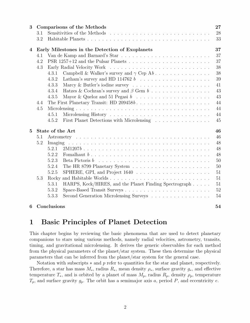
Two mutually orbiting bodies revolve in ellipses about a common center of mass, theorigin of our coordinate system. Orbital angles in the plane of the bodies’ mutual orbit aremeasured with respect to the line of nodes, formed by the intersection of the orbital planewith the plane of the sky (i.e. the plane perpendicular to a line connecting the observer tothe system’s center of mass). The position of this line on the sky has angle Ω, representingthe position angle (measured east of north) of the ascending (receding) node, where the star(and planet) cross the plane of the sky moving away from Earth. Figure 1 illustrates theother orbital elements in the problem. As indicated, the orientation of the each orbital ellipsewith respect to the plane of the sky is specified by the longitude of periastron, ω, which isthe angle between the periastron 1 and the ascending node along the orbit in the directionof the motion of the body. Since the orbit of the star is a reflection about the origin of theorbit of the exoplanet, the orbital parameters of the planet are identical to that of the starexcept that the longitudes of periastron differ by π: ωp = ω∗ + π.

The physical size of the ellipse, given by the semi-major axis, a, is set by Newton’smodification of Kepler’s third law of planetary motion:

P 2 =4π2

G(M∗ +Mp)a3 (1)

The semimajor axis is a = a∗ + ap, where a∗ and ap are the semi-major axes of the twobodies’ orbits with respect to the center of mass, given by,

a∗ =Mp

M∗ +Mpa; ap =

M∗

M∗ +Mpa (2)

The position of either body in its orbit about the origin can be expressed in polar coor-dinates (r, ν), where ν is the true anomaly, the angle between the location of the object andthe periastron. The separation between the star and planet is given by

r(1 + e cos ν) = a(1− e2) (3)

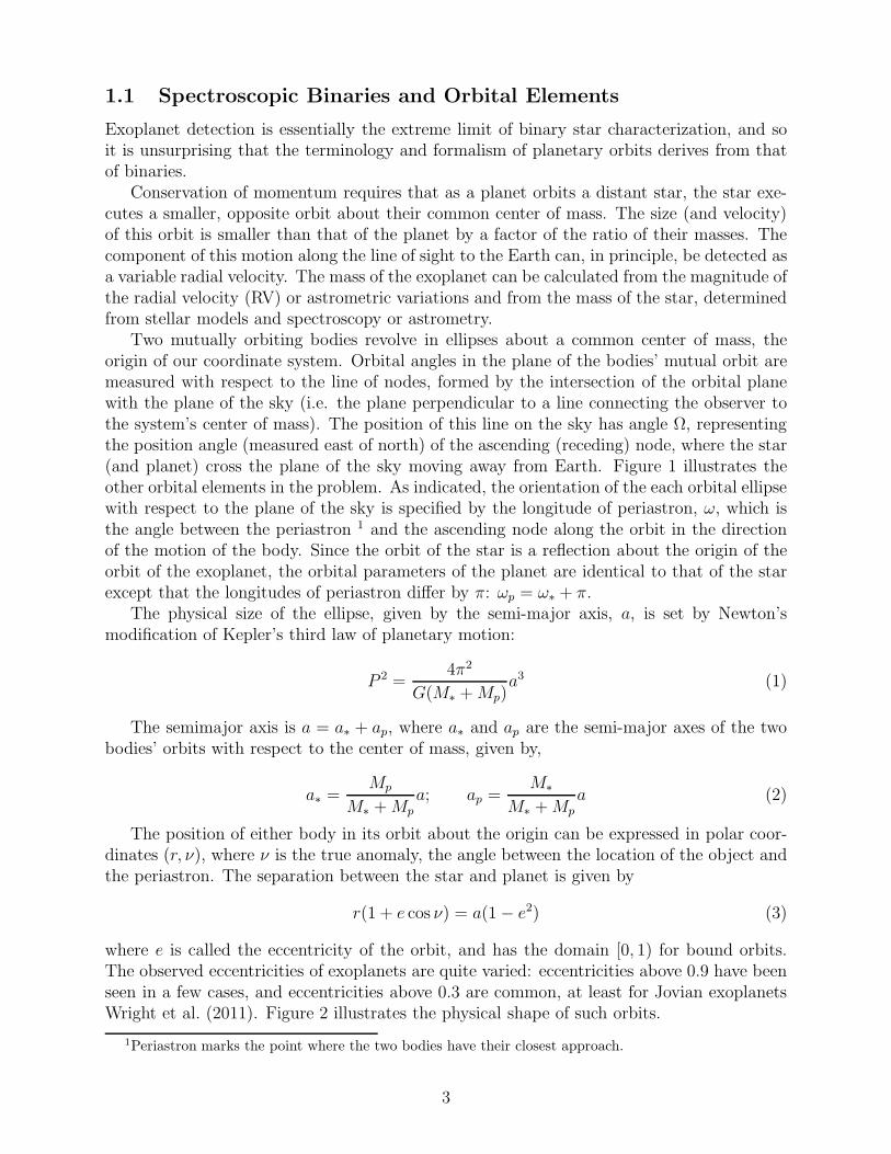
where e is called the eccentricity of the orbit, and has the domain [0, 1) for bound orbits.The observed eccentricities of exoplanets are quite varied: eccentricities above 0.9 have beenseen in a few cases, and eccentricities above 0.3 are common, at least for Jovian exoplanetsWright et al. (2011). Figure 2 illustrates the physical shape of such orbits.

1Periastron marks the point where the two bodies have their closest approach.

3

Mp

r

M* ω*

ν

To observer

Plane of sky

Figure 1: Elements describing orbital motion in a binary with respect to the center of mass(cross). The argument of periastron ω is measured from the ascending (receding) node, andthe true anomaly ν is measured with respect to the periastron. Both angles increase alongthe direction of the star’s motion in the plane of the orbit. The longitude of the periastronof the star ω∗ is indicated. At a given time in the orbit, the true anomalies of the planetand star are equal, where as the longitude of periastron of the planet is related to that ofthe star by ωp = ω∗ + π. In Doppler planet detection, the orbital elements of the star areconventionally reported, from which the orbital elements of the planet can be inferred.

4

−2 −1 0 1 2−1.5

−1.0

−0.5

0.0

0.5

1.0

1.5

e=0

e=0.9

e=0.6

e=0.3

Figure 2: Shape of various eccentric orbits in the orbital plane. A handful of exoplanets witheccentricities above 0.9 have been detected.

5

Practical computation of a body’s position in its orbit with time is usually performedthrough the intermediate variable E, called the eccentric anomaly. E is related to the timesince periastron passage T0 through the mean anomaly, M :

M =2π(t− T0)

P= E − e sinE (4)

.and allows the computation of ν through the relation

tanν

2=

√

1 + e

1− etan

E

2(5)

The eccentric anomaly is also useful because it is simply related to r:

E = arccos1− r/a

e(6)

1.2 Radial Velocities

The radial reflex motion of a star in response to an orbiting planet can be measured throughprecise Doppler measurement, and this motion reveals the period, distance and shape of theorbit, and provides information about the orbiting planet’s mass. (The treatment of RV andastrometric measurement below follows Wright & Howard (2009)).

Six parameters determine the functional form of the periodic radial velocity variationsand thus the observables in a spectroscopic orbit of the star: P , K, e, ω∗, T0, and γ (it isconvention in the Doppler-detection literature to refer to ω without its ∗ subscript, but it isstandard to report the star’s argument of periastron, not the planet’s).

Vr = K[cos(ν + ω∗) + e cosω∗] + γ (7)

with ν related to P , e, and T0 through E. The semi-amplitude of the signal in units ofvelocity is K (the peak-to-trough RV variation is 2K). The bulk velocity of the center ofmass of the system is given by γ.

For circular orbits e = 0, there is no periastron approach, and so T0 and ω∗ are formallyundefined; in such cases a nominal value of ω∗ (such as 0 or π/2) sets T0 (alternatively, onecan specify the value of one of the angles at a given epoch).

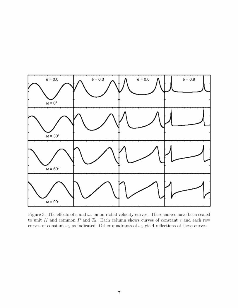
In short, the variables P , T0, and K respectively set the period, phase, and amplitudeof an RV curve, while the variables ω∗ and e determine the shape of the radial velocitysignature of an orbiting companion, as shown in Figure 3. Characterization of the orbits ofsingle unseen companions, such as exoplanets, is ultimately an exercise in fitting observedradial velocities to the family of curves in Figure 3 to determine the six orbital parameters.

Two additional orbital parameters complete the description of a planet’s orbit: the incli-nation of the orbit, i, which determines the angle between the orbital plane and the planeof the sky, such that i = 0 corresponds to a face-on, counter-clockwise orbit, and Ω, thelongitude of the ascending node. These parameters cannot be determined with radial ve-locity observations alone, and can only be measured through astrometry, where the angulardisplacement of the star on the sky is directly measured.

6

ω = 0o

e = 0.0 e = 0.3 e = 0.6 e = 0.9

ω = 30o

ω = 60o

ω = 90o

Figure 3: The effects of e and ω∗ on on radial velocity curves. These curves have been scaledto unit K and common P and T0. Each column shows curves of constant e and each rowcurves of constant ω∗ as indicated. Other quadrants of ω∗ yield reflections of these curves.

7

The effect of the inclination of the orbit is to reduce the radial component of the velocityof the star by sin i. The fundamental observable of a spectroscopic binary which constrainsthe physical properties of system is thus

PK3(1− e2)32

2πG=

M3p sin

3 i

(Mp +M∗)2(8)

where G is Newton’s gravitational constant. The right hand side of this equation is knownas the mass function of the system. For exoplanets where M∗ can be estimated from stellarmodels, the minimum value for Mp (i.e. its value for sin i = 1, or an edge-on orbit) is calledthe “minimum mass” of the planet, and is usually labeled “Mp sin i” for succinctness (sincewhen Mp ≪ M∗ its small correction to the denominator is negligible, though not ignored).The true mass of the detected exoplanet is thus higher by a factor of 1/ sin i, which has atypical (median) value of 1.15 for randomly oriented orbits (all other things being equal).

1.3 Astrometry

Plane-of-sky variations in a star’s position provide both redundant and complementary in-formation to radial velocities, yielding the true inclination and orientation of a planetaryorbit. Astrometry of the orbits of well-separated binary stars of similar magnitude is a mat-ter of careful instrument calibration to precisely measure the separation and position anglebetween the stars. For exoplanet detection, the problem is to detect the motions around astar about an unseen companion with respect to a set of (presumably) stable backgroundstars.

For an orbit with semimajor axis a∗ of a star at distance d from the Earth, producing anastrometric signal of semi-amplitude θ∗ = a∗/d, astrometric orbits can be described in termsof the Thiele-Innes constants

A = θ∗( cos Ω cosω∗ − sinΩ sinω∗ cos i) (9)

B = θ∗( sin Ω cosω∗ + cos Ω sinω∗ cos i) (10)

F = θ∗(− cos Ω sinω∗ − sinΩ cosω∗ cos i) (11)

G = θ∗(− sin Ω sinω∗ + cosΩ cosω∗ cos i) (12)

C = θ∗ sinω∗ sin i (13)

H = θ∗ cosω∗ sin i (14)

which can be quickly computed using rotation matrices:

A B CF G H

θ∗ sin i sin Ω −θ∗ sin i cosΩ θ∗ cos i

= θ∗Rz(ω∗)Rx(i)Rz(Ω) (15)

where R is the 3-D rotation matrix, given in the case of the z-axis by

Rz(Ω) =

cosΩ sin Ω 0− sinΩ cosΩ 0

0 0 1

(16)

8

The Thiele-Innes constants are related back to Keplerian orbital elements with the rela-tions:

tan(ω∗ + Ω) =B − F

A+G(17)

tan(ω∗ − Ω) =−(B + F )

A−G(18)

tan2

(

i

2

)

=(A−G) cos(ω∗ + Ω)

(A+G) cos(ω∗ − Ω)(19)

θ∗ = (A cosω∗ − F sinω∗) cosΩ−(A sinω∗ + F cosω∗) sinΩ sec i

(20)

θ2∗ = A2 +B2 + C2 = F 2 +G2 +H2 (21)

The quantities ω∗ and Ω have a ±π ambiguity that is resolved with radial velocity measure-ments, without which convention dictates that we choose Ω < π.

The C and H constants are related the radial component of the motion. These constantscan be combined with the elliptical rectangular coordinates, defined as

X = cosE − e (22)

Y =√1− e2 sinE (23)

to describe the astrometric displacements of a star in the North (∆δ) and East (∆α cos δ)directions:

∆δ = AX + FY∆α cos δ = BX +GY

(24)

and the magnitude of the astrometric offset from the apparent center of mass is (for small off-sets) ∆θ∗ ≡ [∆δ2 + (∆α cos δ)2]1/2. In practice, astrometric motions are small perturbationson the much larger parallactic and proper motions.

1.4 Imaging

The direct detection of planets is the most conceptually straightforward method of detection:essentially one seeks simply to directly detect photons from the exoplanet, resolved from thoseof the parent star. Although the emission of exoplanets is indeed quite faint, it is generallythe problem of detecting this emission in the proximity of the much brighter stellar sourcethat presents the most severe practical obstacle to direct detection. The disentangling ofstellar and planetary photons is an imperfect process that is easiest at wider separations.The efficiency of this disentangling ultimately determines the detection thresholds of aninstrument. Therefore, the most important parameters of the exoplanet for determiningthe difficulty of direct detection are the planet/star flux ratio fp and the angular separationbetween the planet and star. Typically, contrast limits worsen at smaller angular separations.

The angular separation of the planet and star on the sky is given by

∆θ = r⊥/d (25)

where r⊥ is the projected separation of the planet from the star, and d is the distance to thesystem. By definition, if d is in parsecs and r⊥ in AU, then θ is in arcseconds. In general,

9

∆θ = (1 +M∗/Mp)∆θ∗ = (1 +M∗/Mp)√

(BX +GY )2 + (AX + FY )2. For circular orbits,this reduces to r⊥ = a(cos2 β + sin2 β cos2 i)1/2, where β = ν + ωp is the angle betweenthe position of the planet along its orbit relative to the ascending node. Planets typicallyorbit stars at distances from hundredths to hundreds of AU. For a hypothetical giant planetorbiting 5 AU from a nearby star sitting at 50 pc, this corresponds to a maximal angularseparation of 100 mas.

The emission from an exoplanet can generally be separated into two sources: stellaremission reflected by the planet surface and/or atmosphere, and thermal emission from theplanet. Thermal emission can be due to either “intrinsic” thermal emission (e.g. the fossilheat of formation), or thermal emission from reprocessed stellar luminosity. Exoplanets mayalso produce some non-thermal emission, which we will not consider here.

The reflected light will have a spectrum that is broadly similar to that of the star,with additional features arising from the planetary surface and/or atmosphere. Therefore,for solar-type stars, this reflected emission generally peaks at optical wavelengths. Themonochromatic planet/star flux ratio for reflected light can generally be written (e.g., Seager2010),

fref,λ = Ag,λ

(

Rp

a

)2

Φref,λ(α) (26)

where Ag,λ is the monochromatic geometric albedo, and Φref ,λ is the reflected light phasecurve, which depends on the planetary phase angle α (the star-planet-observer angle) andthe wavelength λ. The geometric albedo is defined as the ratio of the flux emitted from theplanet at α = 0 relative to that of a perfectly and isotropically scattering uniform disk ofequal solid angle. For a circular orbit, cosα = sin β sin i.

Assuming that the thermal emission from the planet has a roughly blackbody spectrum,the flux ratio is

ftherm,λ =

(

Rp

R∗

)2Bλ(Tp)

Bλ(T∗)Φtherm,λ(α) →

(

Rp

R∗

)2Tp

T∗

Φtherm,λ(α), (27)

where Φtherm,λ is the monochromatic thermal phase curve. For observations in the Raleigh-Jeans tail of the blackbody, λ ≫ hc/(kbT ), and thus Bλ(T ) ∝ T , yielding the limit shown inEquation 27. If the planet is in thermal equilibrium with the stellar radiation, then Tp = Teq

andTeq

T∗

=

(

R∗

a

)1/2

[f(1− AB)]1/4, (28)

where AB is the Bond albedo, the fraction of the total energy incident on the planet thatis not absorbed, and f accounts the fraction of the entire planet surface over which theabsorbed energy is re-emitted, i.e. f = 1/4 if the thermal energy is emitted over the entire4π of the planet. Of course, planets may be self-luminous as well, particularly if they areyoung and have retained significant residual heat from formation.

The form for Φref,λ depends on the scattering properties of the planetary atmosphere.For the case of a Lambert sphere that scatters all incident radiation equally in all directions,

ΦLambert,λ =1

π[sinα + (π − α) cosα]. (29)

Also for a Lambert sphere, AB = 1 and Ag = 2/3. The form for Φtherm,λ depends on thesurface brightness distribution of the planet, which in turn depends on the amount of heat

10

redistribution. For the case of a tidally-locked planet in which the absorbed radiation ispromptly and locally re-emitted, the phase curve has the same form as for a Lambert sphere(Seager 2010).

Resolved emission of an planet/star system is essentially equivalent to a visual binary.Once the overall scale of the system has been set, measurements of the position of theplanet relative to the star at a sufficient number of epochs yield all of the orbital elementsof the system, up to the 2-fold degeneracy in orientation with respect to the sky discussedpreviously. The scale of the system can be set either by an estimate of the distance tothe system, or by an external estimate of the primary mass M∗ (under the assumptionMp ≪ M∗). For reflected light measurements, only the product of the geometric albedoand planet cross section can be determined; estimating the planet radius independentlygenerally requires an assumption about the albedo. For thermal light measurements, thetemperature Tp can (in principle) be estimated from the flux at multiple wavelengths, andthen the surface brightness can be estimated from Tp, and thus the radius can be inferredfrom the planetary flux. The planet mass cannot be determined from the planet flux orits relative orbit, and must be inferred indirectly through coupled atmosphere/evolutionarymodels. In some favorable cases, mutual gravitational perturbations in multiplanet systemsmay allow the determination of the planet masses directly.

Of course, the real power of direct imaging lies in the ability to acquire spectra of theplanets once they are discovered, and thus characterize the constituents of the planetaryatmosphere. This provides one of the only feasible routes to assessing the habitability ofterrestrial planets in the Habitable Zones (Kasting et al. 1993) of the parent stars, andlikely the only feasible route to do so for Earthlike planets orbiting solar-type stars.

1.5 Transits

The presence of a planetary companion to a star gives rise to a multitude of physical phe-nomena that manifest themselves via temporal variations of the flux of the system relativeto that of an otherwise identical isolated star. Typically the largest of these occurs if a fortu-nate alignment allows a planet to transit (pass in front of) its host star from our perspective.In this case, the star will exhibit brief, periodic dimmings which signal the presence of theplanet. Transits offer a intriguingly simple way to detect planets.

The condition for a transit is roughly that the projected separation between the planetand host star at the time of inferior conjunction of the planet is less than the sum of the radiiof planet and star, i.e., r(tc) cos i ≤ R∗+Rp, where r(tc) is the separation of the planet fromthe host star at conjunction, and R∗ and Rp are the radii of the star and planet, respectively.Given the definition of ω∗, r(tc) = a(1 − e2)/(1 + e sinω∗), and so transits occur when theimpact parameter of the planet’s orbit with respect to the star in units of the host radius,

b ≡ a cos i

R

1− e2

1 + e sinω∗

, (30)

is less than the sum of the (normalized) radii, b ≤ 1 + k, where k ≡ Rp/R∗ Integratingover i assuming isotropic orbits and thus a uniform distribution of cos i yields the transit

probability,

Ptr ≡(

R∗ +Rp

a

)

1 + e sinω∗

1− e2. (31)

11

For a circular orbit and assuming k ≪ 1, this reduces to the simple expression Ptr = R∗/a.Note that in these expressions, we have used the longitude of the periastron of the orbitof star rather than the (perhaps more intuitive) value for the planet, because the former isgenerally adopted for fits to the stellar reflex radial velocity data.

When the planet transits in front of its parent star, the flux of the star will decreaseby an amount that is proportional to the ratio of the areas of the planet and star. For thepurposes of exposition, in the following we will assume a circular orbit, uniform host surfacebrightness, and Rp ≪ R∗ ≪ a and Mp ≪ M∗. In the general case of a limb-darkened star,eccentric orbit, and arbitrary scales for Rp, R∗ and a, the expressions for the shape of thetransit are considerably more complicated, as are the arguments for the kinds of informationthat can be extracted from transit and RV signals (see Winn 2010 and references therein).However, the basic structure of the problem is the same under our approximations, and whatfollows serves to illustrate the essential concepts.

Under these assumptions, the planet follows a rectilinear trajectory across the face ofthe star with an impact parameter b, and the transit signature will have an approximatelytrapezoidal shape, which can be characterized by the duration T , ingress/egress time τ , andfractional flux depth δ. The depth of the transit relative to the out-of-transit flux is

δ = k2. (32)

The duration of the transit can be quantified by its full-width at half-maximum, which isroughly the time interval T between the two points where the center of the planet appearsto touch the edges of the star. This is approximately,

T ≃ Teq(1− b2)1/2, (33)

where is useful to define the equatorial crossing time (i.e, the transit duration for b = 0),

Teq ≡R∗P

πa= ftrP ≃

(

3P

π2Gρ∗

)1/3

. (34)

Here ρ∗ is the mean density of the host star, and ftr ≡ P/πa = Ptr/π is the transit duty cycle,or the fraction of planet orbit in transit. The last equality, which assumes Mp ≪ M∗, alsoimplies that, to an order of magnitude, the equatorial transit duration is the cube root of theproduct of the orbital period and the stellar dynamical or free-fall time (tdyn ∼ (Gρ∗)

−1/2)squared.

The ingress/egress time (these are equal for a circular orbit) τ is the time between whenthe edge of the planet just appears to touch the star for the first and second time (ingress,or the time between first and second “contact”) or third and fourth time (egress, the timebetween third and fourth “contact”), and is given by,

τ ∼ Teqδ1/2(1− b2)−1/2. (35)

One of the most useful aspects of transiting planets is that, when combined with radialvelocity data, they allow one to infer the masses and radii of the star and planet up to aone-parameter degeneracy, as follows. Measuring T , t, and δ from a single transit allows oneto infer b, Teq, and k

b2 = 1− δ1/2T

τ, T 2

eq =Tτ

δ1/2, k = δ1/2, (36)

12

The impact parameter is related to the orbital inclination i via b = a cos i/R∗, but a and R∗

cannot be determined from light curves alone. With the detection of multiple transits, onecan further infer the period P , and thus the stellar density ρ∗ via Equation 34. As reviewedin §1.2, the reflex radial velocity orbit of the star allows one to infer K and P which can becombined to determine the mass function, ∼ (M∗ sin i)

3/M2/3∗ , but a determination of the

planet mass requires both a measurement of i and M∗. Thus one additional parameter isneeded to break the degeneracy and set the overall scale of the system. This can be accom-plished by imposing external constraints on the properties of the primary, either throughparameters measured from high-resolution spectroscopy or parallax, or invoking theoreticalrelations between the mass and radius of the star through isochrones, or both. For illustra-tion, if we assume the primary mass is precisely known, then we can infer R∗ through ρ∗,and a through P , and thus determine i from the impact parameter measurement. Finally,we can measure Rp from k, and the planet mass from the mass function, i, and M∗.

1.6 Gravitational Microlensing

The gravitational microlensing method detects planets via the direct gravitational pertur-bation of a background source of light by a foreground planet. When a foreground compactobject (either a star or stellar remnant) happens to pass very close to our line-of-sight to amore distant star, the light from the background star will be split into two images. Theseimages are typically unresolved, but they are magnified by an amount that depends onthe angular separation between the lens and source. Since this separation is a function oftime, the background source exhibits a smooth, symmetric time-variable magnification: amicrolensing event. If the foreground lens happens to have a planetary companion and theplanetary companion happens to have a projected separation from the primary lens near thepaths of the two primary images, the gravity of the planet will further perturb the light,resulting in a short-lived perturbation from the primary microlensing event, revealing theplanetary companion. Free floating planets and planets widely separated from their parentstar can also be detected as isolated, short timescale microlensing events.

Consider a planet/star system acting as a lens located at a distance d and source locatedat a distance ds. Light from the source is deflected, split into multiple images, and magnifiedby the gravity of the foreground lens. The fundamental equation that is used to derive theobservable properties of a gravitational microlensing event is the lens equation, which relatesthe angular separation β between the lens and source in the absence of lensing to the angularpositions θ of the images of the source created due to lensing. For a general lens system,these are vector quantities, but for a single lens the lens, source, and image positions are allco-linear, so we can drop the vector notation. The lens equation for an isolated point lens is(Einstein 1936),

β = θ − 4GM∗

c2drelθ, (37)

where d−1rel ≡ d−1 − d−1

s . If the lens and source are perfectly aligned (β = 0), the source isimaged into a ring of radius equal to,

θE ≡(

4GM∗

drelc2

)1/2

≃ 713 µas

(

M

0.5M⊙

)1/2(drel

8 kpc

)−1/2

. (38)

13

The Einstein ring radius is the fundamental scale of gravitational microlensing, and dependson the distances to the lens and source, and the mass of the lens. At the distance of thelens, the linear Einstein ring radius is

rE ≡ θEd ≃ 2.85AU

(

M∗

0.5M⊙

)1/2 (ds

8 kpc

)1/2 [x(1− x)

0.25

]1/2

, (39)

where x ≡ d/ds.Normalizing by θE, the lens Equation 37 simplifies to,

u = y − y−1, (40)

where u ≡ β/θE and y ≡ θ/θE. If u 6= 1, this has two solutions, y± = ±12(√u2 + 4 ± u),

and thus in general an isolated point lens creates two images. One of these images is alwaysseparated by more than θE from the lens (y+ ≥ 1), and the other is always separated byless than θE (|y−| ≤ 1). The separation between the two images is ∼ 2θE and thus they aretypically unresolved. Because the images are distorted relative to the source, they are also(de-)magnified. The total magnification for the sum of the two unresolved images is,

A(u) =u2 + 2

u√u2 + 4

. (41)

The magnification increases for decreasing u (better source-lens alignment), and formallydiverges as u → 0 for a point source.

The source, lens, and observer are all in relative motion, and thus the angular separationbetween the source and lens is a function of time: a microlensing event. If we approximatethe relative proper motion µrel of the lens and source as constant, then we can parametrizethe trajectory of the source relative to the lens as,

u(t) =

[

(

t− t0tE

)2

+ u20

]1/2

, (42)

where u0 is the dimensionless angular separation at the time of closest approach to the lens(the impact parameter), t0 is the time when u = u0 (also the time of maximum magnificationfor a point lens), and tE is the Einstein ring crossing time,

tE ≡ θEµrel

. (43)

Figure 4 shows the source positions, image positions, and magnification of an examplesingle lens microlensing event with u0 = 0.2. In general, the magnification as a functionof time for a single lens event has a smooth, symmetric form that is described by threeparameters (tE, t0, u0). Events with lower u0 lead to more distorted images and highermagnification near peak. For u0 ≪ 1, the peak magnification is Amax ∝ u−1

0 . Events withAmax & 100 are typically referred to as “high magnification events.”

Planetary companions to the lens star can be detected in a microlensing event if theyhappen to have a projected separation in the paths of one or both of the images created bythe primary lens. As the image sweeps by the planet, the gravity of the planet will further

14

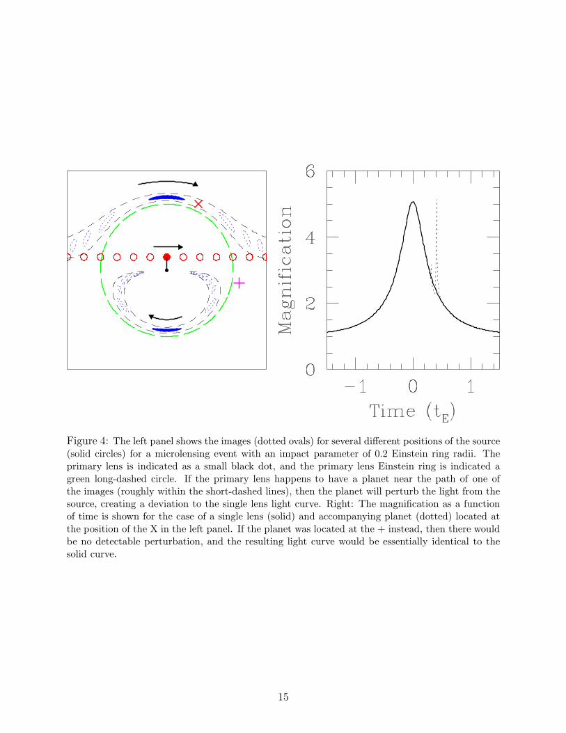
Figure 4: The left panel shows the images (dotted ovals) for several different positions of the source(solid circles) for a microlensing event with an impact parameter of 0.2 Einstein ring radii. Theprimary lens is indicated as a small black dot, and the primary lens Einstein ring is indicated agreen long-dashed circle. If the primary lens happens to have a planet near the path of one ofthe images (roughly within the short-dashed lines), then the planet will perturb the light from thesource, creating a deviation to the single lens light curve. Right: The magnification as a functionof time is shown for the case of a single lens (solid) and accompanying planet (dotted) located atthe position of the X in the left panel. If the planet was located at the + instead, then there wouldbe no detectable perturbation, and the resulting light curve would be essentially identical to thesolid curve.

15

perturb the light from the source associated with the image, creating a short-lived deviationfrom the single-lens form (Mao & Paczynski 1991; Gould & Loeb 1992).

Unfortunately, there are no simple analytic expressions relating the observable featuresof planetary perturbations to the underlying physical parameters of the planet and host star.Adding another body to the lens system increases the complexity of the lensing behaviorsignificantly, and in particular inverting the lens equation for a binary lens to obtain theimage positions for a given source position cannot be done analytically. Furthermore, thebinary gravitational lens has a rich and complex phenomenology, which we will not attemptto explore in this brief review. We refer the reader to more comprehensive summaries by(Bennett 2008; Gaudi 2012). Here we will simply provide a qualitative discussion of planetdetection with microlensing.

Three additional parameters are required to uniquely specify the light curve due to abinary lens (of which star/planet lenses are a subset). The planet/star mass ratio q = Mp/M∗

and instantaneous projected separation s = r⊥/rE between the planet and star in units ofrE at the time of the event together specify the magnification structure of the lens, i.e., themagnification as a function of the (vector) source position u ≡ β/θE. Finally, the parameterα (not to be confused with the phase angle) describes the orientation of the source trajectoryrelative to the projected planet/star axis. Thus a total of six parameters (tE, t0, u0, q, s, α)describe the magnification as a function of time for a binary lens and are thus genericallyobservable.

Single lens microlensing events yield only one parameter that depends on the physicalproperties of the lens star, namely the time scale tE. The time scale provides only a weakconstraint on the lens mass, because it depends not only on the mass, but also on the lensand source distances, and the relative lens-source proper motion, all of which are relativelybroadly distributed for a typical microlensing survey. In addition, the lens stars are typicallyquite faint and are blended with other stars (including the lensed source). Thus little isgenerally known about the host star properties. Planetary microlensing events generallyyield two parameters that are related to the planet properties, q and s. While q is ofinterest in its own right, s is generally not, because it depends on the phase, orientation,and eccentricity of the orbit, as well as on the Einstein ring radius, all of which are a prioriunknown. Therefore, s is only weakly correlated with the semimajor axis of the orbit, andprovides essentially no constraint on the other orbital elements.

Although this “baseline” situation sounds quite dire, in fact it has been shown that withadditional effort, it is possible to obtain substantially more information about the host star,planet, and its orbit for the majority of detected systems using a combination of subtle,higher-order effects that are detectable in precise microlensing light curves, and follow-uphigh-resolution imaging in order to isolate the light from the lens (Bennett et al. 2007).

1.7 Timing

A star or stellar remnant that exhibits regular, periodic photometric variability, such aspulsars, pulsating white dwarfs, eclipsing binary stars, pulsating hot subdwarfs, or evenstars with transiting planets, can show evidence of a planetary companion through timingvariations in those periodic phenomena. There are three principle sources of such variations:the Doppler shift, light travel time, and gravitational perturbations.

The first of these sources is exactly analogous to the radial velocity method, but measures

16

changes in frequencies of some property other than photons. If the period of the pulsationsor eclipses can be measured to sufficient precision, then the interpretation of those variationsis identical to that in the radial velocity method.

The light travel time effect comes about when the reflex orbit of a star about the centerof mass of the star-planet system is sufficiently large that the additional light travel timeacross this orbit is detectable as a timing variation. This is not a truly distinct phenomenonfrom the Doppler shift timing method, since it is essentially the accumulated effects of theDoppler-shifted period that produce the timing anomaly. Depending on the period of theintrinsic variation and the physical size of the star’s reflex orbit, either effect, or both, maybe detectable.

The above methods have been most successfully employed with pulsars (through the pulsearrival times) and eclipsing binary systems (through the timing of eclipse ingress and egress),and was responsible for the detection of the first exoplanets (Wolszczan & Frail 1992).

Finally, in the case of an eclipsing system, such as an eclipsing binary or a transitingplanet, additional bodies in the system will perturb the orbits of the eclipsing bodies. Theseperturbations can be especially large if the perturbing body is near a mean motion resonancewith the other bodies. When applied to systems of transiting planets this method is calledtransit timing variations (TTVs, Agol et al. 2005; Steffen & Agol 2005; Holman & Murray2005), and has been most successfully employed by Kepler (e.g., Ford et al. 2012).

2 The Magnitude of the Problem

By almost any physical measure, planets are small in comparison to their parent stars, andthe observable phenomena that are used to directly or indirectly detect them are likewisesmall. In this section, we attempt (where possible) to provide order-of-magnitude estimatesof the precisions of the relevant observations that are required to detect planets using variousmethods. We then use these estimates, along with additional requirements imposed by thespecifics of the detection method (i.e, the detection efficiencies), to provide a broad outline ofthe practical requirements that must be met for planet surveys to successfully detect planetswith a given set of properties.

In general, specifying the criteria needed to detect a planet requires a detailed analysisof the signal and data properties, as well as a quantitative definition of the meaning of adetection. However, for many of the detection methods, a rough estimate can be obtained bydecomposing the primary observable signal into two conceptually different contributions: anoverall scale and detailed signal waveform. The overall scale, which depends on the physicalparameters of the system, encodes the order-of-magnitude of the signal and largely dictatesits detectability. The waveform itself depends on more subtle details of the system (i.e., theprecise shape of the planet orbit), but typically takes on values of order unity and thus hasa relatively small effect on the detectability of the signal. Therefore, in most cases, thesetwo contributions can be fairly cleanly separated. In this approximation, the detectability ofa planet with a given set of properties therefore primarily depends primarily on the overallsignal scale, and the data quality and quantity, i.e., the typical observational uncertaintiesand the total number of observations. With this in mind, given a signal amplitude A,number of observations N , and typical measurement uncertainty σ, the detectability will

17

depend primarily on the total signal-to-noise ratio S/N, which scales as,

S/N ≃ g√NA

σ(44)

where g is a factor of order unity that depends on the details of the signal.

2.1 Radial Velocities

The differential radial velocity signal of a planet has the form ∆Vr = KF (t; e, ω∗, T0, P ),where F (t) encodes the detailed shape of the RV signal. Assuming uniform and densesampling of the RV curve over a time span that is long compared to P , and assuming a totalof N observations each with measurement uncertainty σRV , the total signal-to-noise ratio is

(S/N)RV ≃ g(e, ω∗)√N

K

σRV. (45)

For a circular orbit, g = 2−1/2, and is generally a weak function of e for e . 0.6. Forlarger eccentricities, g declines gradually, but more importantly the stochastic effects of fi-nite sampling become significant for typical values of N (e.g., O’Toole et al. 2009; Cumming2004). For planets with periods larger than the duration of the observations, the detectabil-ity depends additionally on the period and phase of the planet, and generally decreasesdramatically with increasing period, typically as (S/N)RV ∝ P−1 (e.g., Eisner & Kulkarni2001; Cumming 2004).

Thus, a robust detection of a planet via RV typically requires achieving radial velocityprecisions of σRV ≪ KN1/2. For Mp ≪ M∗, the semiamplitude K is,

K =

(

P

2πG

)−1/3Mp sin i

M2/3∗

(1− e2)−1/2 (46)

Thus to detect a true Jupiter analog (i.e. a Jupiter-mass planet in a 11.8 yr, circular orbitaround a Solar-mass star), for which K ≃ (12.5 m/s) sin i, requires a few dozen observationswith precisions of a few m/s. An RV precision of 3 m/s corresponds to a Doppler shift of

K/c ≃ 10−8. The motion induced by an Earth analog is smaller by a factor of 318/(11.8)13 ∼

100, so requires an additional two orders of magnitude in precision.Typically the centroid of stellar spectral lines at fixed equivalent width can be measured

with a precision of ∝ σ3/2V /N

1/2eff , where σV is the effective velocity width of the spectral

line and Neff is the effective number of photons in the line (i.e., the equivalent width ofthe line times the photon rate per unit wavelength). Maximizing the precision requiresthat the lines are well-resolved, and thus that the instrumental velocity resolution is lessthan the intrinsic velocity width of the star. For reference, the typical width of a spectralfeature in a slowly rotating star is of order a few km/s (∼ 10−5), and thus resolving powersof (R = ∆λ/λ ∼ 105) are needed, comparable to the resolving power of a typical high-resolution astronomical echelle spectrograph. The velocity precision per line is generallyinsufficient to detect planetary companions, and thus averaging over many lines is required.The statistical signal-to-noise ratio requirements are quite stringent, and thus bright starsand/or large apertures are generally needed.

18

Because the velocity precisions needed to detect planetary companions are well belowthe intrinsic widths of the spectral lines and even below the velocity precisions that can beobtained for individual lines, getting close to the photon limit requires excellent control ofsystematics. One of the most severe requirements is that the wavelength calibration mustbe both more precise than the desired velocity precisions, and stable over many times theorbital period of the planet. For a Jupiter analog, this wavelength calibration must be ata level of better than 10−3 of a resolution element, and stable over the course of decades.Since the Earth’s motion about the Sun imparts a periodic Doppler shift of order 30 km/s(v/c = 10−4), this accuracy and precision must be maintained even as the spectral linesmove annually by 104 times the measurement precision.

There are at least two proven2 paths to surmounting this challenge: though preciseinstrumental calibration with an absorption cell (the iodine technique), and through instru-mental ultra-stability (as exemplified by HARPS), both of which are briefly described in§§4.3.1–4.3.5.

2.2 Astrometry

The magnitude of the differential astrometric offset of a star at a distance d due to a planetarycompanion has the general form ∆θ∗ = θ∗F (t; e, ω∗, i, T0, P ), where the semi-amplitude ofthe astrometric offset for a circular, face-on orbit is,

θ∗ ≡a

d

Mp

M∗

, (47)

and we have assumed Mp ≪ M∗. Again assuming uniform and dense sampling of theastrometric curve over a time span that is long compared to P , and assuming a total of Nobservations each with measurement uncertainty σAST , the total signal-to-noise ratio is

(S/N)AST ≃ g(e, ω∗, i)√N

θ∗σAST

. (48)

We note for simplicity we have assumed that each observation yields a given uncertaintyσAST on the magnitude of the vector position of the star relative to some reference frame;in reality each of these measurements may require a separate measurement for each of thetwo orthogonal directions. For e = 0, g(i) = [0.5(1 + cos2 i)]1/2. For more general cases, thebehavior of g is qualitatively similar to that for radial velocity signals. For e 6= 0, g dependsadditionally on ω∗ and e, but is a relatively weak function of e for e . 0.6. However, theeffects of finite sampling start to become more important as e increases, particularly for lowN . When P is greater than the span of observations, the detectability also depends on T0

and P , generally decreasing rapidly with increasing period, also typically as P−1.The magnitude of the astrometric signal of a Jupiter analog orbiting a nearby solar-type

star at a distance of D ∼ 20 pc is θ∗ ≃ 0.25 mas, whereas for an Earth analog the astrometricwobble is over 1500 times smaller, or around 0.15 µas. Thus astrometric precisions of order

2Another technique, externally dispersed interferometry (EDI Erskine & Ge 2000), has shown promiseas a third path to precise velocimetry. It employs an interferometer in front of a spectrograph at modestresolution, generating a known, unresolved, sinusoidal transmission function, somewhat analogous to a gascell’s absorption properties. The phase of the beating of the stellar spectrum against this pattern is a measureof radial velocity.

19

a mas or a µas are needed to detect gas giants or terrestrial planets, respectively. Sinceastrometry is most sensitive to planets orbiting the nearest stars, which have typical propermotions of ∼ 103 mas/yr and annual parallactic motion of ∼ 102 mas, the target starstypically move by more 103 times the required measurement precision over the course of ayear, and secularly at 105 times the measurement precision per decade.

The photon limit of an astrometric measurement of a star depends on the signal-to-noiseratio and width of the point spread function (PSF), and scales as σAST ∼ FWHM/

√N ,

where N is the total number of photons in the measurement. As mentioned previously,diffraction limited PSFs, FWHM ∼ λ/D, where D is either the aperture of the telescope orthe baseline of the interferometer. Baselines of . 100m therefore yield single measurementprecisions of . 4mas. Therefore, the astrometric detection of planets generally relies on theability to achieve both nearly photon-limited performance when measuring the centroid ofindividual images, and the ability to average many individual measurements to improve thefinal precision. As is the case with RV, excellent control of systematics is therefore required.There are a number of ways to achieve this, depending on the nature of the observing setup(direct imaging, interferometry, etc.).

Interferometric methods in particular allow precisions below 1 mas from the groundaround bright stars with good, nearby reference stars, putting astrometric exoplanet detec-tion within reach. Much better control of systematics is in principle possible from space, andthus space-based interferometers should be able to achieve precisions of 1–10 µas, makingthem a potential route for the detection of nearby true Earth analogs (Unwin et al. 2008).

2.3 Imaging

The flux ratio of a planet (or planet/star contrast) at a given wavelength λ and epoch canbe expressed as fλ = f0,λΦ(α), where Φ(α) describes the phase curve, whose form dependson the properties of the planet atmosphere, and is a function of the phase angle α, whichin turn depends on the measurement epoch and orbital elements e, ωp, i, T0, P . The phasecurve typically takes on values . 1, and thus the magnitude of the reflected light signal ischaracterized by f0,λ. This factor depends on the nature of the planetary emission, but forreflected light and thermal emission takes the form (see equations 26 and 27),

f0,λ = Ag,λ

(

Rp

a

)2

(Reflected), f0,λ ≃(

Rp

R∗

)2Tp

T∗

(Thermal), (49)

where the latter equality assumes observations on the Rayleigh-Jeans tail, which yields thelargest flux ratio. Further, for thermal emission arising from reprocessed starlight,

f0,λ ≃(

Rp

R∗

)2(R∗

a

)1/2

[f(1− AB)]1/4 (Thermal,Equilibrium) (50)

The signal-to-noise ratio with which a planet can be directly detected in N measurementsis (Kasdin et al. 2003; Brown 2005; Agol 2007),

(S/N)dir ≃ g√Nf0,λσeff

. (51)

20

Here g = [N−1∑

k Φ(αk)2]1/2

is the root-mean-square of the phase function values at thetimes k of the observations, and σeff is the average effective per-measurement photon noiseuncertainty normalized to the total stellar flux. In the usual background-limited case, theprimary contributions to the uncertainty are residual light from the stellar point spreadfunction, and local and exo-zodiacal light. In the case where the scattered light from thestar is dominant, σeff ∼

√

C/N∗ (Kasdin et al. 2003), where C is the contrast ratio betweenthe intensity of the scattered light from the star in the wings of the point spread functionrelative to the peak, and N∗ is the total number of photons collected from the star in themeasurement.

In contrast to many radial velocity and astrometric surveys, direct imaging surveys aregenerally designed with the requirement that such that the target signal-to-noise ratio per

measurement is & 1 (Kasdin et al. 2003), and thus N ∼ 1. Achieving a sufficient S/N permeasurement then typically translates into a requirement that C . f0,λ, i.e., the flux fromthe planet within a given aperture is larger than the local background from the stellar PSFin the same aperture.

Young (< 1 Gyr old), self-luminous planets can still be quite warm (1000–2000 K),even at arbitrarily large separations from their parent stars, making them in some sensethe easiest targets for direct imaging surveys. For these temperatures and roughly Jupiterradii, the planet/star flux ratios are f0,λ ∼ 10−4–10−6 at near-IR wavelengths, or ∆m ∼10–15 magnitudes. Purely in terms of overall brightness, young exoplanets are rather easilydetectable with large telescopes at infrared wavelengths; the primary difficulty therefore liesin suppressing the residual starlight at the position of the planet in order to achieve thecontrast ratios C needed to distinguishing the planetary light from the star’s.

Since the albedos of exoplanets at distances of & 0.1 AU are typically expected to be oforder unity, the flux ratio of a planet in reflected starlight is f0,λ ∼ (Rp/a)

2. For a Jupiteranalog this is ∼ 10−8 or about 20 magnitudes, whereas for an Earth analog this is ∼ 10−9, orabout 23 magnitudes. The bolometric thermal flux ratio of an exoplanet in equilibrium withthe starlight will be of the same order of magnitude as the reflected light flux ratio, howeverthe monochromatic thermal flux ratio may be substantially larger, since the planet is coolerand so its thermal emission will peak in the Rayleigh-Jeans tail of the stellar blackbodyemission. For a Jupiter analog at ∼ 10µm, f0,λ ∼ 10−8, where as for a Earth analog it isf0,λ ∼ 10−7.

Achieving a given contrast ratio is generally more difficult for small angular separationsfrom the host star, and becomes generally impossible closer than some minimum inner

working angle, θIWA. Thus the angular separation ∆θ = r⊥/d is another important parameterthat determines the detectability of planets by direct imaging. The probability distributionof the projected separation r⊥ given a value of a for random orbital phases and viewinggeometries is generally sharply peaked at a. Thus the typical angular separation of a planetwith a = 5.2 AU orbiting a star at 20 pc is ∼ a/d = 250 mas, whereas it is 50 mas for a = 1AU. The inner working angle typically scales as (and is generally similar to) the diffractionlimit of telescope,

θdiff ∼ λ/D (52)

where D is the diameter of the telescope (or the most widely separated components of aninterferometer). This corresponds to 60 mas at 2 microns on an 8m telescope. Thus, surveysfor Earth analogs are generally only feasible for the nearest stars.

21

The detectability of a planet by direct imaging depends on a complicated interplay be-tween many variables, including the semimajor axis and size of the planet, age and distanceto the star, and wavelength capabilities of the imaging system. For example, for reflectedlight surveys, the orbital separation effects the detectability of the planet through the oppos-ing effects of contrast and angular separation. As another example, while younger planetstend to be more luminous, younger stars are also less common and so typically more dis-tant. Additional factors may also contribute to these interplays, such as the brightness ofthe exozodiacal light as a function of semimajor axis, and variations in the planetary atmo-spheric properties (e.g., albedo and absorption bands) as a function of semimajor axis, age,and surface gravity. Direct imaging surveys therefore need to be designed carefully in orderto maximize the discovery space and so chance of success. Combined with the technicalchallenges associated with achieving the contrast ratios and inner working angles neededfor planet detection briefly described below, it is clear that direct imaging is a generallyexpensive and challenging detection method. Nevertheless, the potential payoff is enormous,particularly when considering the goal of directly imaging Earth analogs.

The technical aspects of imaging exoplanets comprise surmounting three challenges: cor-ralling starlight into a nearly diffraction-limited PSF (and away from the planet image);mechanically blocking the starlight before it can diffract into the planet image; and sub-tracting the remaining starlight at the position of the planet image on the detector to revealthe planet image beneath. These three challenges are most forcefully attacked using adaptiveoptics, coronagraphy, and various forms differential imaging, respectively.

Adaptive optics (AO) refers to controlling the wavefronts of the incoming starlight andplanet-light, which ideally consist of parallel planes propagating toward the telescope. Theatmosphere and telescope optics both introduce aberrations to this wavefront which resultin a PSF that differs significantly from that which a theoretically perfect optical systemwould produce (for an unocculted circular aperture, this would be an Airy function). Formost ground-based telescopes, the primary source of wavefront aberrations is the atmosphere.Adaptive optics use movable or deformable mirrors which can be rapidly actuated in responseto measured atmospheric aberrations, usually at tens to thousands of Hertz. These systemsdramatically reduce the effects of atmospheric blurring, and the best of them can collectmost of a star’s light into the shape dictated by optical diffraction. This heightens the peakof faint sources and reduces noise from the star outside the diffraction limit.

The technique of blocking the light of a bright source to reveal faint surrounding featuresis called coronagraphy. A coronagraph uses a series of masks in an optical system to block,reorganize, or alter the phase of incoming light such that “on-axis” light from the staris almost entirely blocked or caused to destructively interfere, while “off-axis” light (forinstance, from a nearby planet) is relatively unaffected. Because important aspects of thistechnique happen in the pupil plane, stellar photons can be distinguished from planetaryphotons and rejected before they arrive on the same pixels on the detector. The effect isto reduce the contamination from stellar photons at the detector position of the planet,enhancing its detectability outside of the diffraction limit. There has been a proliferationof coronagraph designs in recent years, but they share the common feature of reducing orcontrolling the nature of the diffraction of the light into the planet image.

Adaptive optics systems and coronagraphs are not perfect. Their limitations, the aber-rations introduced by the telescope, and diffraction spikes and rings from the aperture canresult in significant amounts of starlight outside of the diffraction limit. The most insidious

22

of these effects are the semi-static patterns of “speckles” from residual wavefront errors.Differential imaging is the process of precisely determining the PSF of the starlight and at-tempting to subtract it, leaving only the planet light to be detected. In principle, differentialimaging is limited by the quality of the model PSF and the unavoidable photon noise in theresiduals to that model. The reference image being subtracted can be determined from areference star (RDI), or from the data themselves through angular modulation (ADI), spec-tral analysis (SDI), polarization analysis (PDI), or other some other method or combinationof methods.

A conceptual cousin of coronagraphy is interferometry, which allows widely separatedapertures to combine incoming light to form interference fringes whose amplitudes and phasesare sensitive to the presence of faint, off-axis companions. Such work is common at radiowavelengths, and in the infrared can be especially profitable just inside of the traditionaldiffraction limit of the telescope. Two such techniques are aperture masking interferometry,where a single telescope pupil is divided into small sub-apertures and the light is combinedat the focal plane, and nulling interferometry where light from two telescopes is combinedsuch that the starlight undergoes destructive interference, while the planet light, incomingat a slightly different angle, interferes constructively.

2.4 Transits

The fractional change in the flux of a star when it is transited by a planetary companionhas the form ∆F∗/F∗ = −δ F (t;Rp,M∗, R∗, a, i, e, ωp), where δ = k2 is the square of theplanet/star radius ratio, and the function F (t) describes the detailed shape of the transitcurve, and also generally depends on the surface brightness profile of the star. In the case ofcircular orbits, no limb darkening, and Rp ≪ R∗, the form for F (t) can be approximated bya box car with a depth of unity and duration of T = Teq(1− b2)1/2, where Teq and b are theequatorial crossing time and impact parameter, respectively, as defined in §1.5. The fractionof time the planet is in transit (the transit duty cycle) is then ftr = T/P .

Transit surveys generally operate by obtaining many observations of the target stars overa given time span. Of course, in order to be detectable a planet must be favorably alignedsuch that it transits. The transit probability is roughly Ptr ∼ R∗/a. Then, assuming uniformsampling over a time span that is long compared to P , the signal-to-noise ratio of the transitwhen folded about the correct planet period is,

(S/N)tr ≃√

Nftrδ

σph(53)

where N is the total number of observations and σph is the fractional photometric uncertainty.Therefore, the probability of detecting a given planet via transits can be roughly quantifiedby three characteristics of the planetary system that depend primarily on Rp, R∗, and a,

δ =

(

Rp

R∗

)2

, Ptr ∼R∗

a, ftr ∼

Ptr

π, (54)

For a typical hot Jupiter with Rp ≃ RJ and P ≃ 3 days orbiting a solar-type star,the transit probability is Ptr ∼ 10%, the transit depth is δ ∼ 1%, and the duty cycle isftr ∼ 3%. These parameters place Hot Jupiters well within the capabilities of ground-based surveys, although the requirements are not trivial. First, since Hot Jupiters are

23

only found around ∼ 0.5% of solar-type stars (Gould et al. 2006), many thousands of starsmust be surveyed to guarantee a transiting Hot Jupiter. Obtaining relative photometryat precisions of less than a few millimagnitudes for thousands of stars simultaneously fromthe ground is generally difficult, and thus ground-based transit surveys operate close to thelimit where δ/σph ∼ 1. Therefore, hundreds of epochs during transit are needed for robustdetections, corresponding to many thousands of total measurements. Aliasing effects arisingfrom the diurnal constraints make achieving the required number of points in transit morechallenging. All of these requirements are most easily met with relatively small aperture, butvery wide field-of-view telescopes (e.g., Pepper et al. 2003; Bakos et al. 2004; Pollacco et al.2006; McCullough et al. 2005).

In fact, finding transiting planets in wide-field surveys has proven even more difficult thansimply meeting these (already difficult) requirements. First, wide-field transit surveys mustcontend with a huge fraction of false positives in the form of grazing eclipsing binaries (EBs),eclipsing binaries blended with brighter stars, and more exotic variables. Furthermore, eventhose signals that are consistent with a Jupiter-sized transiting object can, in principle, bemuch more massive companions, since the radius of compact objects is essentially constantfrom the mass of Saturn through ∼ 0.1M⊙ (e.g. Burrows et al. 1997). Thus radial velocityfollow-up is need to eliminate these false positives. Finally, high-precision (few m/s) radialvelocity follow-up is needed to precisely measure the planet mass. The most successfulsearches achieve reliably high photometric accuracy over large fields, and employ multiplesites with good longitudinal coverage, sophisticated and automated transit identificationalgorithms, and thorough follow-up campaigns that using multi-band photometry, multi-band astrometry (to rule out close, chance alignments of EBs and foreground stars) , andradial velocity work. Further characterization of a transiting planet is most successfully doneusing photometry and high signal-to-noise ratio spectroscopy with larger ground and/or spacetelescopes.

The requirements for the detection of Earth analogs orbiting solar-type stars are especiallychallenging. In this case, the fractional transit depth is ∼ 10−4, the transit probability is∼ 0.5%, and the duty cycle is ∼ 0.1% (i.e., the planet transits for T . 13 hours once ayear). The detection of transiting Earth analogs requires essentially continuous observationsof hundreds of stars, and precisions of better than ∼ 0.1 mmag for periods of several years.These requirements cannot be met from the ground, and require space-based photometricmonitoring. Indeed, the Kepler mission was designed to detect such planets, achieving therequired photometric precision to detect Earth-sized planets on tens of thousands of stars(Borucki et al. 2010, see also § 5.3.2).

Transiting planets can also be found via photometric follow-up of known radial velocitycompanions; indeed the first transiting planet was discovered in this way (Henry et al. 2000;Charbonneau et al. 2000). Here the challenges are somewhat different than the “traditional”method of discovering transiting planets through their photometric signature. First, theprobability that a given radial velocity companion will also transit its parent star is low,. 10%. Second, radial velocity searches have traditionally been limited to relatively brightstars, and so the total number of stars have targeted for precision RV searches is ∼ 103,making the total yield of transiting planets from this sample also low. Furthermore, achievingphotometry at the level of precision needed to detect the transit signature may be challengingfor very bright stars, primarily because of the lack of suitable comparison stars. Finally, theuncertainties in the predicted times of inferior conjunction from the radial velocity fits can

24

be quite large, from several hours to several days. Nevertheless, seven transiting systemshave been discovered amongst the sample of companions first discovered via radial velocity,and there are ongoing projects that aim to increase this sample by first refining the radialvelocity emphemerides of promising systems, and then performing photometric follow-up(Kane et al. 2009).

2.5 Microlensing

Unlike the detection methods discussed above, the signals caused by planetary companionsin microlensing events cannot be described analytically except in a few specific limits thatare not generally applicable. Nevertheless, we can provide some qualitative guidelines andapproximate scaling behaviors that will elucidate the general requirements for successfulsurveys for planets with microlensing. We stress that, because of the large diversity in theproperties of the systems that give rise to gravitational microlensing events, the expressionsprovided should be treated as very rough estimates only.

A somewhat unusual attribute of the microlensing method is that the magnitude of amicrolensing perturbation does not depend on the properties of the planet in the generalcase. Rather, the magnitude depends primarily on the angular separation of the planet fromthe image(s) it is perturbing. However, the duration of the planetary perturbation doesdepend on the planet properties, in particular the mass ratio q. Very approximately, theduration of the planetary deviation is ∆tp ∼ q1/2tE, where tE is the primary event time scale.The primary event light curves must be sampled on a time scale significantly smaller than∆tp in order to detect and characterize the planetary perturbation. Furthermore, the detec-tion probability also depends on the planet mass ratio, such that Pdet ∼ 20%(q/0.001)∼5/8

(Horne et al. 2009). This detection probability is averaged over a uniform distribution of im-pact parameters, and is appropriate for planets with projected separations that are withina factor of ∼ 2.6 of the Einstein ring radius, r⊥ ∼ [0.6 − 1.6]dθE, sometimes called the“lensing zone”. Planets with separations much smaller or much larger than this range havesubstantially lower probability of detection. As discussed in the context of direct imaging,the distribution of projected separation r⊥ for random viewing geometries and orbital phaseis sharply peaked at r⊥ ∼ a.

In addition, there is a minimum mass that can be detected in microlensing surveys, thatis set by the finite size of the source stars. When the angular size of the planet perturbationregion is substantially smaller than the angular size of the source, the planet perturbs onlya small fraction of the source, and the magnitude of the resulting deviation is stronglysuppressed. A rough limit on the mass ratio can be established by when the angular sizeof the source θ∗ is a factor of ∼ 3 times larger than the angular Einstein ring radius of theplanet θp = q1/2θE, corresponding to roughly an order of magnitude suppression of the planetsignal. Thus qmin ∼ 0.1ρ2∗, where ρ∗ ≡ θ∗/θE (Gould & Gaucherel 1997).

Thus the parameters that determine the detectability of planets with microlensing are

∆tp ∼(

Mp

M∗

)1/2

tE, Pdet ∼ 20%

(

Mp/M∗

0.001

) 5/8

, a ∼ [0.6−1.6]dθE, qmin ∼ 0.1ρ2∗,

(55)where the parameters tE, and ρ∗ additionally depend on the mass and distance to the host starvia the angular Einstein ring radius (see Eq. 38). The distributions of M∗, tE, d, and θE for

25

microlensing events toward the Galactic bulge are quite broad, but we can take typical valuesof M∗ ≃ 0.5 M⊙, tE ≃ 25 days, d ∼ 4 kpc, and θE ∼ 0.7 mas. Thus microlensing planetsurveys are most sensitive to planets with semimajor axes of a ≃ [1− 5] AU(M/0.5 M⊙)1/2.For a Jupiter-mass planet, the typical planet perturbation duration is ∆tp ∼ 1 day, andthe typical detection probability is ∼ 30% in the lensing zone. For an Earth-mass planet,∆tp ∼ 1.5 hours, whereas the detection probability in the lensing zone is ∼ 1%.

The typical dimensionless source size for a clump giant star (∼ 13 R⊙) in the Galacticbulge is ρ∗ ∼ 0.01, whereas for a turn-off star (∼ R⊙) it is ∼ 0.001. Thus the minimum massratio that can be detected by monitoring clump giant sources is qmin ∼ 10−5, correspondingto ∼ 1.7× mass of the Earth for a typical primary lens of 0.5 M⊙. For main sequencestars in the bulge, qmin ∼ 10−7, corresponding to just over the mass of the Moon! Thusdetecting planets with mass of the Earth or less requires monitoring main-sequence stars.The difficulty lies in the fact, in the crowded fields toward the Galactic bulge, most mainsequence stars are severely blended with other unrelated background stars in typical ground-based seeing conditions, dramatically increasing the photometric noise. Therefore, detectingplanets with mass substantially less than that of the Earth generally requires a space-basedsurvey (Bennett & Rhie 2002; Bennett 2008).

A final difficulty with in microlensing surveys is the low overall event rate of gravitationalmicrolensing events. Toward the Galactic bulge, the rate of microlensing events is roughlyΓ ∼ 10−5 per star per year (e.g., Kiraga & Paczynski 1994). Thus, in order to detect ∼ 103

events per year (the current number of microlensing events that are detected per year towardthe Galactic bulge by the Optical Gravitational Lensing Experiment (OGLE) collaboration3),of order 100 million source stars must be monitored. There are 3 million stars per squaredegree down to an I magnitude of 19 in Baade’s window (Holtzman et al. 1998), whereI ∼ 19 is roughly the peak of the distribution of baseline magnitude for microlensing events.Thus several tens of square degrees of the bulge must be monitored.

The unpredictability of microlensing events requires monitoring the potential source starswith a cadence that is substantially smaller than the timescale of interest. For the primarymicrolensing events, which have a typical tE ∼ 25 days, this means roughly daily observa-tions. Detecting the planetary perturbations on these events requires much higher cadencesof a few hours or less. Furthermore, since the total durations of the planetary perturbationsare of order a day or less, networks of longitudinally-distributed telescopes must be em-ployed in order to avoid missing part or all of the perturbations. Given these requirements,traditional microlensing planet surveys have used a two-tier approach, where collaborationswith dedicated access to telescopes with a relatively wide fields of view of ∼ 0.5− 2 squaredegrees monitor the tens of square degrees needed to detect the primary microlensing events,but with cadences that are generally insufficient to detect planetary perturbations on theseevents (Udalski 2003; Sako et al. 2008). These survey collaborations alert the microlensingevents real-time before the peak magnification, thus allowing “follow-up” collaborations withaccess to narrow-angle telescopes on several continents to monitor only a subset of the starsthat display ongoing microlensing events with the cadences needed to detect planetary per-turbations (Albrow et al. 1998; Tsapras et al. 2009; Dominik et al. 2010; Gould et al. 2010).Future surveys will operate on a very different principle, as described in §5.3.3.

3See http://ogle.astrouw.edu.pl/ogle4/ews/ews.html.

26

2.6 Timing

The magnitude of the signal in other planet detection techniques varies. Timing for mil-lisecond pulsars like PSR 1257+12 can in principle detect extremely low mass objects (sig-nificantly < 1M⊕) given a sufficient amount of data, limited primarily by pulsar timingnoise.

Other timing techniques, such as eclipsing binary times or pulsating hot subdwarfs, relyon timing variations being correctly interpreted as a light-travel time effect of a star or stellarsystem orbiting a common center of mass with an unseen companion. A summary of suchdetections is listed in Schuh (2010); most of these detections imply minimum companionmasses of several times that of Jupiter. The sensitivities of these methods is difficult todetermine, however, since they depend on the magnitude of all non-orbital origins in tim-ing variations, which have not been well quantified. Most of the current detections are offewer than two full apparent orbits (periods are 3–16 yr) and so the strict periodicity thatis characteristic of Keplerian signals cannot yet be confirmed. Further, quasi-cyclical timingvariations may be generated by poorly understood internal mechanisms such as the “Ap-plegate effect” (Applegate 1992). Following these apparent planetary systems for multipleorbits will help illuminate the true sensitivities of these methods.

Transit timing variations (TTVs) provide an extremely sensitive method of detecting newplanets or characterizing known planets in a transiting system. The sensitivity is a complexfunction of the orbital parameters of the planets involved, but is optimized when the planetsare in mean-motion resonances (Veras et al. 2011). Kepler is sufficiently precise in its timingto measure variations of order minutes in the ingress and egress times of transiting planets,which in principle allows it to reach mass precisions of order 1 M⊕ over several years ofobservation.

In known multi-transit systems, these variations can be used to infer the masses of theplanets involved (e.g. Lissauer et al. 2011) and in apparently single systems they can beused to detect non-transiting planets (e.g. Ballard et al. 2011). Ground-based planet transittiming will generally be limited to precisions of a tens of minutes, and so have correspondinglyweaker sensitivities.

3 Comparisons of the Methods

In the previous sections, we reviewed the primary exoplanet detection methods in somedetail, outlining the principles of each method, including the primary physical observablesand practical challenges associated with achieving robust detections. In this section, we placethese discussions in the context of the larger goal of constraining exoplanet demographicsby outlining the regions of planet and host star parameter space where each method is mostsensitive. When then compare the methods with one another in this context, highlightingthe strong complementarity of the methods. We also briefly discuss and compare how theintrinsic sensitivity of each method to planets in the Habitable Zones of their parent starsscales with host star mass.

The sensitivity of the various detection methods as a function of planet mass and sepa-ration is illustrated in Figure 5. We show the masses and semimajor axes of the exoplanetsdiscovered by radial velocities, direct imaging, timing, transits, and microlensing, as of Dec.

27

2011. In addition, we show estimates of the sensitivity of various surveys using radial ve-locities, direct imaging, transits, microlensing, and astrometry. In the following subsection,we explain the scaling of these survey sensitivities with planet parameters, and explain ourspecific choice for their normalization. Host star mass is a third parameter that can stronglyinfluence the sensitivity of these methods, but is suppressed in this figure. Therefore, inorder to provide a somewhat fairer comparison across the broad range of host star massesrepresented in this figure, we normalize the semimajor axis by an estimate of the snow linedistance (e.g., Kennedy & Kenyon 2008),

asl = 2.7 AUM∗

M⊙. (56)

The snow line is the location in the protoplanetary disk where the temperature is below thesublimation temperature of water. In the currently-favored paradigm of planet formation,the snow line distance plays an important role, as the larger surface density of solids beyondthe snow line facilitates giant planet formation, whereas primarily rocky planets are expectedto form interior to the snow line (e.g., Lissauer 1987; Pollack et al. 1996; Ida & Lin 2004;Mordasini et al. 2009).

Both the locations of the known planets and the regions of sensitivity in Figure 5 serve toillustrate the complementarity of the various detection methods. In particular, radial velocityand transit surveys are most sensitive to relatively short-period exoplanets with separationsinterior to the snow line. State of the art surveys using these methods are sensitive toplanets as small as the Earth. In contrast, direct imaging and microlensing surveys are mostsensitive to planets beyond the snow line. Current direct imaging surveys are sensitive to verywidely-separated, massive planets. Current and near-term microlensing surveys are sensitiveto planets with masses greater than that of the Earth, whereas a space-based microlensingsurvey would be sensitive to planets with mass greater than that of Mars and separationsgreater than a few AU, including free-floating planets. The combined sensitivity of currentand proposed surveys using the methods discussed in the chapter encompasses an extremelybroad volume of parameter space, including planets with masses greater than that of theEarth for arbitrary separations (including free-floating planets), host stars with masses fromthe bottom of main sequence to several times the mass of the sun, and distances from thesolar neighborhood to the Galactic center. Thus the full complement of these methods canpotentially provide a nearly complete picture of the demographics of exoplanets.

3.1 Sensitivities of the Methods

• Radial Velocities. The radial velocity signal and signal-to-noise ratio scales as

(S/N)RV ∝ MpP−1/3M−2/3

∗ ∝ Mpa−1/2M−1/2

∗ . (57)

Thus, at fixed host star mass, RV surveys are generally more sensitive to more massiveplanets, and have a weak preference for shorter-period planets, at least for periodsshorter than the span of the measurements. At fixed S/N, the minimum detectable

mass scales as Mp,min ∝ P 1/3M2/3∗ ∝ a1/2M

1/2∗ . This mass limit is shown in Figure

5 assuming M∗ = M⊙ and a minimum detectable RV signal of K ∼ 1 m/s (i.e.,corresponding to a (S/N)RV ∼ 10 detection with 100 observations each with single

28

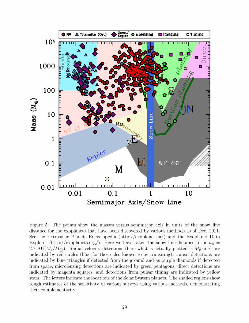
Figure 5: The points show the masses versus semimajor axis in units of the snow linedistance for the exoplanets that have been discovered by various methods as of Dec. 2011.See the Extrasolar Planets Encyclopedia (http://exoplanet.eu/) and the Exoplanet DataExplorer (http://exoplanets.org/). Here we have taken the snow line distance to be asl =2.7 AU(M∗/M⊙). Radial velocity detections (here what is actually plotted is Mp sin i) areindicated by red circles (blue for those also known to be transiting), transit detections areindicated by blue triangles if detected from the ground and as purple diamonds if detectedfrom space, microlensing detections are indicated by green pentagons, direct detections areindicated by magenta squares, and detections from pulsar timing are indicated by yellowstars. The letters indicate the locations of the Solar System planets. The shaded regions showrough estimates of the sensitivity of various surveys using various methods, demonstratingtheir complementarity.

29

measurement precisions of ∼ 1m/s.). In principle, sufficiently massive planets can bedetected even when they have periods longer than the duration of observations, howeverit will generally not be possible to uniquely measure Mp sin i and P in these cases, andthus the usefulness of such ‘detections’ are significantly compromised. Therefore, wesimply assume an upper limit on the period of P = 2000 days.

At fixed planet properties, the RV signal increases with decreasing host star massesas M

−2/3∗ . However, there are many additional factors that enter into the overall de-

tectability as a function of mass, through the radial velocity uncertainty σRV . At fixeddistance to the host star, the velocity uncertainty due to photon noise increases withdecreasing mass for main-sequence stars, both because of the strong mass-bolometricluminosity relation for main-sequence stars, and because of the difficulties of continuumnormalization in very cool stars, where most RV surveys are carried out. The intrinsicvelocity information in stellar spectra also varies as a function of spectral type. In par-ticular hot (Teff & 6500K) stars have few spectral lines and typically rotate much morerapidly than cooler stars with convective envelopes. Finally, the astrophysical radialvelocity noise (i.e., “jitter” due to spots) also depends on spectral type and stellar age(Wright 2005). When taken together, these factors tend to favor late G or early Kquiet main-sequence stars as the most promising for detecting low-mass planets (e.g.,Pepe et al. 2011).

• Astrometry. The astrometric signal and signal-to-noise ratio scales as

(S/N)AST ∝ MpP2/3M−2/3

∗ d−1 ∝ MpaM−1∗ d−1, (58)

and so at fixed stellar mass, astrometric surveys are more sensitive to massive, long-period planets. At fixed S/N, the minimum detectable mass scales as Mp,min ∝P−2/3M

2/3∗ d ∝ a−1M∗d. This limit is shown in Figure 5 assumingM∗ = M⊙ and d = 10

pc, and a minimum detectable astrometric signal θ∗ ≃ 0.35 µas (i.e., a (S/N)AST ∼ 5detection with 200 2-D observations each with σAST ∼ 1 µas precision). As with radialvelocity observations, although it is possible detect the astrometric signal of planetswith period larger than the duration of observations, it is generally not possible toindependently measure the mass and orbital parameters with observations that do notcover a complete orbit. This is particularly problematic for astrometric observations,because in this regime the signal of the proper motion of the star is partially degener-ate with the astrometric signal of the planetary companion. Astrometric surveys aretherefore expected to have the most sensitivity to planets with periods similar to thesurvey duration, and increasing the survey duration has a strong effect on the surveyyield.

At fixed planet properties and host star distance, the astrometric signal increases withdecreasing host star mass as M

−2/3∗ . Stellar spots are generally not expected to be

an important source of astrometric noise (Makarov et al. 2009), and thus the onlyadditional dependence of the sensitivity of astrometric surveys on stellar mass entersthrough the effects of the typical distance and photon noise uncertainty of the hoststars. Specifically, low-mass stars are more common and thus have a smaller typicaldistance, but are less luminous and thus yield poorer astrometric precision.

30

• Imaging.

For direct detection in reflected and equilibrium thermal emission light, the planet/starflux ratio and thus the signal-to-noise ratio scales as

(S/N)dir ∝ R2pa

−2 (Reflected), (59)

(S/N)dir ∝ R2pTpR

−2∗ T−1

∗ (Thermal) (60)

(S/N)dir ∝ R2pR

−3/2∗ a−1/2 (Thermal,Equilibrium), (61)

where the last two forms again assume observations in the Rayleigh-Jeans tail. Theother primary requirement for direct imaging is that the angular separation between theplanet and star is larger than inner working angle, and thus a & θIWAd

−1. Thus at fixedprimary properties and distance, larger and hotter planets are more readily detectable.As discussed in §2.3, the dependence of detectability on semimajor axis is not trivial:planets with larger orbits generally have smaller flux ratios, however they must have anangular separation greater than the inner working angle to be detectable. Furthermore,additional effects that are likely to depend on the planet semimajor axis may affectthe detectability, such as the variation of the planetary albedo with separation.

At fixed planet properties, the signal-to-noise ratio with which a planet can be detectedin reflected light is largely independent of the host star properties. For detection inthermal emission, larger and/or hotter host stars generally give rise to smaller fluxratios. The other effect of host star mass enters through the dependence on distance:less massive host stars are more numerous and so have a smaller average distance,whereas more massive host stars are more luminous and thus give rise to smallerphoton noise uncertainties at fixed distance. Finally, the age of the host star plays animportant role in the detectability of planets, particularly with current surveys: young,self-luminous planets have flux ratios that are both larger than would be expected forplanets whose emission is dominated by reflected light or equilibrium thermal emission,and are independent of their semimajor axis. Thus relatively luminous planets withseparations well beyond the inner working angle can be found around young stars.

Current ground-based imaging surveys are most sensitive to young, massive (Mp &

MJUP) self-luminous planets with semimajor axes of & 10 AU around the neareststars. Thus these surveys are sensitive to planets in a regime of parameter space thatis not currently being probed by other methods. We illustrate the current region ofsensitivity of imaging surveys in Figure 5, assuming planets with Mp & MJUP anda & 10 AU can be detected. Future surveys (some of which will be initiated very soon)will be sensitive to a much broader region of planet parameter space.

• Transits Assuming uniformly-sampled observations over a time span T that is longcompared to the planet period, the signal-to-noise ratio with which a transiting planetcan be detected scales as

(S/N)tr ∝ R2pP

−1/3M−5/3∗ ∝ R2

pa−1/2M−3/2

∗ , (62)

where we have assumed R∗ ∝ M∗, as appropriate for stars on the main sequencewith M . M⊙. In addition, the transit probability scales as Ptr ∝ P−2/3M

2/3∗ ∝

31

a−1M∗, and the requirement to detect at least n transits sets a strict lower limit onthe period P ≤ T/n. Thus for fixed host star properties, the sensitivity of transitsurveys is strongly weighted toward short period, large-radius planets. At fixed S/N,

the minimum detectable planet radius scales as Rp,min ∝ P 1/6M5/6∗ ∝ a1/4M

3/4∗ . For

planets with a constant density, this translates into a minimum mass of Mp,min ∝R3

p,min ∝ P 1/2M5/2∗ ∝ a3/4M

9/4∗ . This limit is shown in Figure 5, assuming a minimum

(S/N)tr = 8 and a mid-latitude transit and photon noise-limited precision for a M∗ =M⊙, V = 12 star from Kepler (Gilliland et al. 2011). The relatively strong dependenceof the signal-to-noise ratio on planet radius, combined with the decreasing transitprobability with increasing planet period, generally implies that the yield of a transitsurvey is a relatively weak function of the total duration T .

Main-sequence stars are clearly the best targets for transit searches. At fixed planetradius and period, low-mass main-sequence stars yield larger transit signals. However,for photon noise limited uncertainties, the signal-to-noise ratio also depends on thestellar luminosity in the wavelength of the observations, and the distance to the star.Low-mass stars are more common, and are therefore are closer on average. Thesenet result of these various countervailing effects on the scaling of the sensitivity oftransit surveys with host star mass depends on the survey parameters, particularly thewavelength, target field, and magnitude limit (Pepper & Gaudi 2005). All-sky surveysin the visual at fairly bright magnitudes tend to be dominated by F and G stars(Pepper et al. 2003), but surveys for fainter stars, or surveys in near-IR wavelengths,tend to be more heavily weighted to toward low-mass stars.

• Microlensing

As discussed previously, microlensing surveys are less amenable to analytic characteri-zation of the sensitivity and scaling with planet and host star parameters. Nevertheless,we have the general qualitative result that the sensitivity peaks for semimajor axes thatare similar to the Einstein ring of the host star lens, aopt ∼ 2.85 AU(M∗/0.5M⊙)1/2.Both the detection probability at fixed semimajor axis and range of sensitivity aroundthis peak increases for larger mass ratio. The range of planet mass and semimajor axisto which a given microlensing survey is most sensitive depends on the details of thesurvey design, in particular the number and peak magnification of the primary eventsthat are monitored, and the precision and cadence of the observations. In Figure 5, weshow representative estimates for the sensitivity of a current ground-based microlensingsurvey based on the analysis of Gould et al. (2010), a next-generation ground-basedsurvey as described in §5.3.3, and a space-based survey similar to WFIRST as de-scribed Green et al. (2011). Generally, current microlensing surveys are most sensitiveto planets with Mp & 10 M⊕, with separations just beyond the snow line spanning afactor of a few in semimajor axis. Next generation ground-based surveys will lower thesensitivity in mass by roughly an order of magnitude to Mp & M⊕, and broaden therange of semimajor axis by a factor of ∼ 2. A space-based survey would be sensitiveto planets with mass greater than the mass of Mars with separations greater than afew AU, including analogs to all of the solar system planets except Mercury.

Because microlensing does not rely on the detection of photons from the host star, thesensitivity of a microlensing survey to the host star parameters enters primarily through

32

the microlensing event rate as a function of host star mass. The microlensing eventrate is given by the integral of the number density of lenses along the line of sight to thebulge, weighted by the cross section for lensing, which depends on the host star Einsteinring radius (∝ M

1/2∗ ) and its projected transverse velocity. Figure 6 shows a theoretical

estimate of the microlensing event rate toward the Galactic bulge, as a function of thelens mass. The sensitivity of microlensing planet surveys is roughly proportional tothis event rate. Thus microlensing surveys are sensitive to main-sequence hosts withmass from below the hydrogen burning limit up to the turn-off of the stellar population(∼ M⊙), as well as remnant hosts. The sensitivity to brown dwarf and main-sequencehosts is roughly constant per logM∗.

3.2 Habitable Planets

Of particular interest is the detection of terrestrial planets in the Habitable Zones of theirparent stars. In §2, we discussed the magnitude of the signal expected for an Earthlikeplanet separated by one AU from a solar type star for various detection methods. Thesesignals are generally quite small. However, we can and should also consider the signals anddetectability of Earthlike planets orbiting in the Habitable Zones of main-sequence starswith mass significantly different than the sun. Because the masses, radii, and luminositiesof stars on the main sequence can span an order of magnitude or more, both the location ofthe Habitable Zone and the magnitude of the signal expected from an Earthlike habitableplanet can vary substantially.

In this subsection, we derive the scaling of the detectability of Earthlike habitable planetswith host star mass. To this end, we adopt a power-law form for the stellar mass-bolometricluminosity relation,

L∗

L⊙

∼(

M∗

M⊙

)4

. (63)

Our adopted exponent of 4 roughly corresponds to that found from a weighted fit to thedata for benchmark binary systems analyzed in Torres et al. (2010). This form provides areasonable approximation of this data set over the full span of masses of ∼ 0.2M⊙− 50M⊙.We note, however, that there are significant deviations from this form within the range,particularly for stars below the fully-convective boundary, which are generally more luminousthat predicted by Equation 63. Nevertheless, we will adopt this simple form for the purposesof illustration. With this adopted mass-luminosity relation, we can define the location of theHabitable Zone as,

aHZ = AU

(

L∗

L⊙

)1/2

∼ AU

(

M∗

M⊙

)2

, PHZ ∼ yr

(

M∗

M⊙

)5/2

, (64)

Therefore, the Habitable Zone location ranges from a semimajor axis of ∼ 0.01AU and periodof ∼ 1 day for a star at the bottom of the main sequence to ∼ 4 AU and ∼ 6 years for aM∗ ∼ 2 M⊙ star. We adopt a mass-radius relation of the form,

R∗

R⊙

∼ M∗

M⊙(65)

33

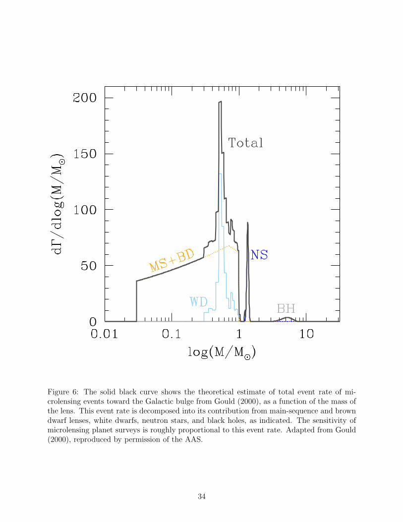
Figure 6: The solid black curve shows the theoretical estimate of total event rate of mi-crolensing events toward the Galactic bulge from Gould (2000), as a function of the mass ofthe lens. This event rate is decomposed into its contribution from main-sequence and browndwarf lenses, white dwarfs, neutron stars, and black holes, as indicated. The sensitivity ofmicrolensing planet surveys is roughly proportional to this event rate. Adapted from Gould(2000), reproduced by permission of the AAS.

34

which describes the data in Torres et al. (2010) reasonably well for non-evolved stars withM∗ . 2M⊙.

With these assumptions, we can now use the results from §3.1 to derive the scaling of thesignal of a habitable planet with host star mass for the various methods we have discussed.

• Radial Velocities. For radial velocity surveys, the radial velocity and signal-to-noiseratio for planets in the Habitable Zone scales as

(S/N)RV ∝ MpM−3/2∗ (Habitable). (66)

Therefore, all else being equal, Habitable Zone planets are significantly easier to detectaround lower-mass stars. In particular, for stars with M . 0.2 M⊙, the radial velocityamplitude for an Earth-mass planet in the Habitable Zone is expected to be & 1m/s,which is within the reach of current instrumentation (Bean et al. 2010).

• Astrometry. The astrometric signal and signal-to-noise ratio for habitable planetsscales as,

(S/N)AST ∝ MpM∗d−1 (Habitable), (67)

and thus at fixed distance and planet mass, astrometric surveys are more sensitive tohabitable planets orbiting higher-mass stars, provided that the period of the planets isless than the duration of the survey. In addition, higher-mass stars are more luminousand thus have smaller photon noise uncertainties. On the other hand, higher-massstars are also less common and thus are typically more distant. The net result of thesefactors is that A and F stars are the most promising targets for astrometric searchesfor planets in the Habitable Zones of nearby stars (Gould et al. 2003a).

• Imaging. For direct detection of habitable planets in thermal equilibrium with theirhost stars, the planet star flux ratio and signal-to-noise ratio scale as,

(S/N)dir ∝ R2pM

−4∗ (Reflected,Habitable), (68)

(S/N)dir ∝ R2pM

−5/2∗ (Thermal,Habitable), (69)

strongly favoring low-mass stars. Note that, by definition, the amount of stellar ir-radiation for a planet in the habitable zone is independent of the mass of host star,and thus for fixed planet properties the thermal or reflected flux of the planet is alsoindependent of the mass of the host star. The dependence on stellar mass in the abovescaling relations therefore arises simply from the change in the flux of the star. How-ever, the second requirement for direct detection is that the angular separation of theplanet from its parent star must be larger than the inner working angle of system. Atfixed mass, this translates into a maximum distance that a Habitable Zone planet canbe detected,

dmax = 10 pc

(

θIWA

100 mas

)−1(M∗

M⊙

)2

(Habitable). (70)

The number of available targets is ∝ n(M∗)d3max, where n(M∗) is the volume density of

stars of a given mass, i.e., the mass function. Since the exponent of the mass function

35

in the local solar neighborhood is generally & −2, this requirement strongly favorshigh-mass stars. The optimal mass will depend on the precise details of the survey andthe nature of the noise sources (see, e.g., Agol 2007), but these arguments demonstratethat we can generically expect the sensitivity of imaging surveys for habitable planetsto be fairly strongly peaked at intermediate masses.

• Transits. The signal-to-noise ratio, transit probability, and period of a transitinghabitable planet scale as,

(S/N)tr ∝ R2pM

−5/2∗ , Ptr ∝ M−1

∗ , P ∝ M5/2∗ , (Habitable) (71)

all of which favor or strongly favor low-mass stars. Furthermore, as discussed above,the radial velocity signals of Habitable Zone planets around low-mass stars are alsolarger and within reach. Finally, low-mass stars are more common. These variousconsiderations have led to the suggestion that transit surveys of low-mass stars may bethe most promising route to detecting habitable Earthlike planets (Gould et al. 2003b;Nutzman & Charbonneau 2008; Blake et al. 2008). Indeed, several such surveys areunderway or are being planned (e.g., Charbonneau et al. 2009), with the ultimate goalof finding a Earthlike system whose atmosphere can be characterized with, e.g. theJames Webb Space Telescope (Deming et al. 2009).

• Microlensing. The system parameters which determine the detectability of a givenplanetary system with gravitational microlensing are the mass ratio q and projectedseparation s in units of rE. For a habitable Earthlike planet these are,

q ∼ 5× 10−5

(

Mp

M⊕

)(

M∗

0.5M⊙

)

, (72)

sHZ ≡ aHZ,⊥

rE∼ 0.1

(

M

0.5M⊙

)3/2 (ds

8 kpc

)−1/2 [x(1− x)

0.25

]−1/2

, (Habitable) (73)

where in the expression for sHZ we have assumed a median projection factor such thataHZ,⊥ = 0.866aHZ. Therefore, for typical microlensing host stars, the Habitable Zonedistance is much smaller than the Einstein ring. While mass ratios of q ∼ 10−5 arereadily detectable for planets with separations near the Einstein ring (s ∼ 1), they aremuch more difficult to detect for planets with s ≪ 1. This is because these such planetscan only be detected when they perturb the inner image created by the primary hoststar, and then only when this image is close to the primary and thus highly demagnified.See Figure 4. These perturbations are therefore generally quite small. Furthermore,perturbations of the inner image are more strongly suppressed for large source stars(Gould & Gaucherel 1997; Bennett & Rhie 1996).

From Equation 73, we see that microlensing favors the detection of habitable plan-ets around higher-mass stars (Di Stefano & Night 2008), and stars that are close tothe source or close to the Earth (i.e., such that x(1 − x) is small). While currentand next-generation ground-based microlensing surveys have essentially no sensitiv-ity to habitable Earthlike planets, specialized surveys for nearby microlensing events,or space-based surveys which boast much larger event rates and detection efficien-cies, could potentially detect such systems (Di Stefano & Night 2008; Park et al. 2006;Bennett et al. 2010b; Green et al. 2011).

36

4 Early Milestones in the Detection of Exoplanets

4.1 Van de Kamp and Barnard’s Star

The pre-1995 literature is scattered with several (presumably) spurious claims of detectionsof planets around nearby stars. Perhaps the best known early claim is that of van deKamp, who conducted a astrometric campaign to detect “dark” companions to nearby stars(van de Kamp 1986). Van de Kamp’s lower limits were impressive, typically ruling outJupiter-mass objects in periods of years to a couple decades, and he reported several starsas having barely-detectable companions of apparently substellar mass. Most intriguing washis report of first one, then later two Jupiter-mass companions to Barnard’s star (GJ 699),the second closest stellar system to Earth.

Van de Kamp made astrometric measurements from the positions of the apparent cen-troids of stellar images on photographic plates, and targets such as Barnard’s star sufferedfrom having a constantly changing set of astrometric references over his multi-decade sur-vey due to its record-high proper motion (over 10”/yr). Subsequent astrometric and radialvelocity work have ruled out his claims (Choi et al. 2012, ApJ, submitted, and referencestherein).

4.2 PSR 1257+12 and the Pulsar Planets

Pulsars are exquisite clocks, typically producing pulses with periods of order ∼ 1–10−3 s.Once these periods are corrected for well-measured linear drifts with time and occasional“glitches” (sudden shifts in period), their precision can rival and even surpasses the bestatomic clocks on Earth. Successful analysis of pulse arrival times requires carefully solvingfor the distance and space motion of the pulsar and the removal of the effects of the motionof the observatory.

In 1991, two teams announced having contemporaneously observed unexplained residualsto their timing models indicative of the first known exoplanets: very small, terrestrial-planet-mass companions orbiting their pulsars. Matthew Bailes and Andrew Lyne (Bailes et al.1991) reported a timing variation with a period of 6 months apparently due to a 10 M⊕

companion orbiting the pulsar PSR 1829-10. Meanwhile, Cornell astronomer AlexanderWolszczan had observed a similar sort of signal from a millisecond pulsar, PSR 1257+12,and had recruited Dale Frail of the National Radio Astronomical Observatory to help confirmits position on the sky to perfect the position model. By November 1991 Wolszczan & Frail(1992) had submitted a manuscript on their discovery, and both teams planned to describetheir work at the January 1992 meeting of the American Astronomical Society.

At the meeting, Lyne announced that just days earlier he had discovered an error in histiming model. A tiny positional error combined with an insufficiently precise descriptionof the Earth’s orbit had led to the small, periodic, 6-month signal in their residuals thatthey had mistaken for a planet. With the correct timing model, there was no evidence of aplanetary perturber on the pulsar. Lyne’s public and frank admission was acknowledged asa laudable demonstration of scientific integrity by a standing ovation at the meeting and aneditorial in Nature (Lyne & Bailes 1992; Nature 1992; Wolszczan 2012).

The world would not be long with its first exopanets, however. The very next speakerat the AAS meeting was Wolszczan, whose timing model had correctly accounted for all

37

important effects. Wolszczan described the first planets known outside the solar system: apair of bodies with ∼ 4 M⊕ orbiting the millisecond pulsar PSR 1257+12 with periods of 66and 98 days. This system would continue to impress, revealing a third low mass planet toWolszczan’s team, as well (Wolszczan et al. 2000).

These planets’ formation mechanism is still not understood, and to date no similar systemof low mass planets is known. Signals of higher-mass planets orbiting pulsars would continueto be found, however: in particular, Bailes would go on to discover an apparently high-density1.4 MJup object orbiting pulsar PSR J1719-1438 (Bailes et al. 2011).

4.3 Early Radial Velocity Work

4.3.1 Campbell & Walker’s survey and γ Cep Ab

In the 1981, Bruce Campbell of the University of Victoria, Gordon Walker of the Universityof British Columbia, and their team began an ambitious survey for substellar objects orbiting20 of the brightest nearby stars. They sought to exploit the recently available technologiesof high resolution (R > 40,000) echelle spectrographs and digital detectors in the form ofReticons and CCDs to achieve the best possible Doppler precision.

To establish an accurate and robust wavelength solution they employed an absorptioncell of hydrogen fluoride (HF) which imposed a “picket fence” of regular, strong, narrow, andwidely spaced (∼ 15A) absorption lines from the 3 → 0R branch transitions near 8700A, farfrom any telluric features (Campbell et al. 1988). Campbell & Walker had sought a chemicalcell that would provide such lines in the optical that would not contaminate the stellarlines, and with few extraneous absorption features from isotopic impurities or other effects.Cambell & Walker found no other chemicals that fit their needs, and so used HF despite theserious difficulties of working with that chemical4. To achieve the necessary optical depthand wavelength stability of HF lines, Campbell & Walker stabilized the temperature andpressure of their 1 m long cell at 373 K and connected it to a vessel containing liquid HF inan ice bath, yielding a pressure of roughly 0.5 atm.

The well-known and well-spaced HF lines granted Cambpell & Walker unprecedentedoptical Doppler precision, independent of mechanical and thermal changes in the opticsof their spectrograph. This method was, at the time, greatly superior to emission linecalibration because the reference lines were measured simultaneously to the stellar exposureand through the same optical path as the stellar photons. Cambell & Walker achieved 10–15 m/s radial velocity precision on most of their sample of 20 stars. This precision is, inretrospect, more than sufficient to detect close-in giant exoplanets, but their sample of starswas simply too small and close-in planets are too rare for them to have discovered a strongexoplanetary signal with any significant likelihood.

Campbell et al. (1988) were able to confirm that objects with m sin i = 10–80 MJup arerare, and noted several interesting signals near the limits of their detectability. They notedan especially intriguing apparent signal for γ Cep A with a 25 m/s amplitude and 2.7 yr

4Campbell & Walker understatedly reported the “obnoxious” nature of HF and that “standard safetyprecautions of chemical laboratories are appropriate” for this rather dangerous chemical which is reacts withglass, forms hydrofluoric acid on contact with water, can painlessly penetrate human tissues, and causes burnsthat can necessitate amputation (OSHA Occupational Safety and Health Guidelines for HF, US Departmentof Labor, 2012).

38

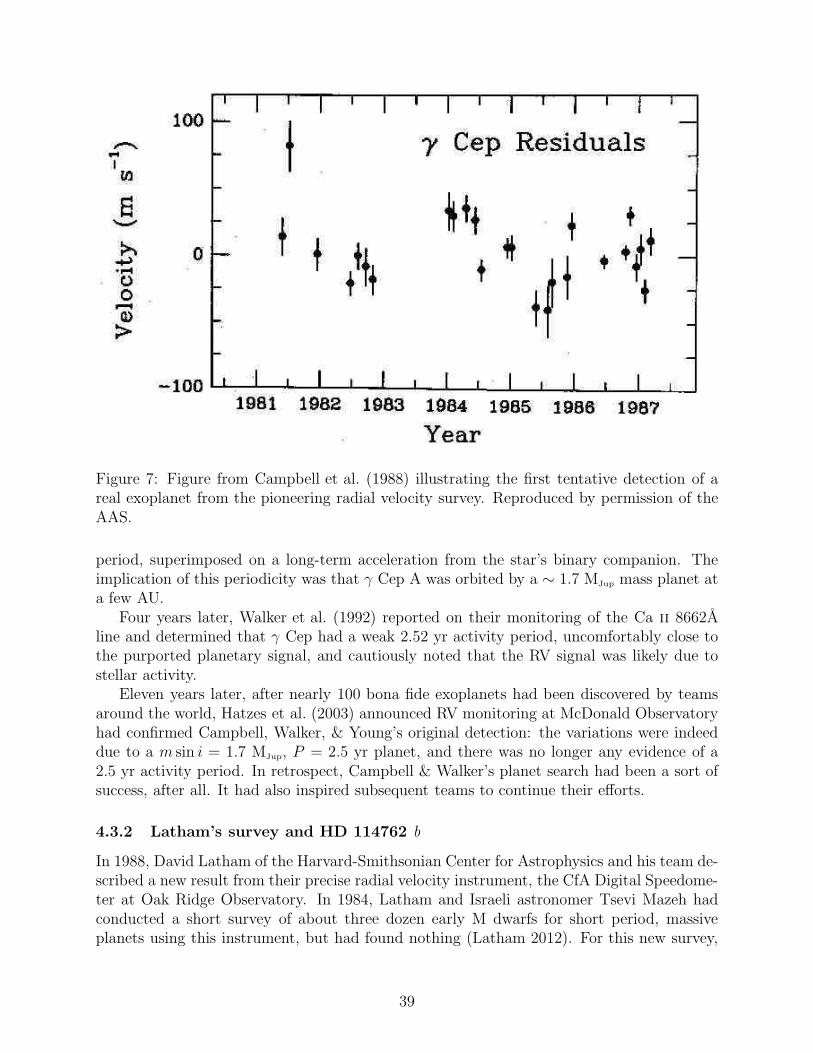
Figure 7: Figure from Campbell et al. (1988) illustrating the first tentative detection of areal exoplanet from the pioneering radial velocity survey. Reproduced by permission of theAAS.

period, superimposed on a long-term acceleration from the star’s binary companion. Theimplication of this periodicity was that γ Cep A was orbited by a ∼ 1.7 MJup mass planet ata few AU.

Four years later, Walker et al. (1992) reported on their monitoring of the Ca ii 8662Aline and determined that γ Cep had a weak 2.52 yr activity period, uncomfortably close tothe purported planetary signal, and cautiously noted that the RV signal was likely due tostellar activity.

Eleven years later, after nearly 100 bona fide exoplanets had been discovered by teamsaround the world, Hatzes et al. (2003) announced RV monitoring at McDonald Observatoryhad confirmed Campbell, Walker, & Young’s original detection: the variations were indeeddue to a m sin i = 1.7 MJup, P = 2.5 yr planet, and there was no longer any evidence of a2.5 yr activity period. In retrospect, Campbell & Walker’s planet search had been a sort ofsuccess, after all. It had also inspired subsequent teams to continue their efforts.

4.3.2 Latham’s survey and HD 114762 b

In 1988, David Latham of the Harvard-Smithsonian Center for Astrophysics and his team de-scribed a new result from their precise radial velocity instrument, the CfA Digital Speedome-ter at Oak Ridge Observatory. In 1984, Latham and Israeli astronomer Tsevi Mazeh hadconducted a short survey of about three dozen early M dwarfs for short period, massiveplanets using this instrument, but had found nothing (Latham 2012). For this new survey,

39

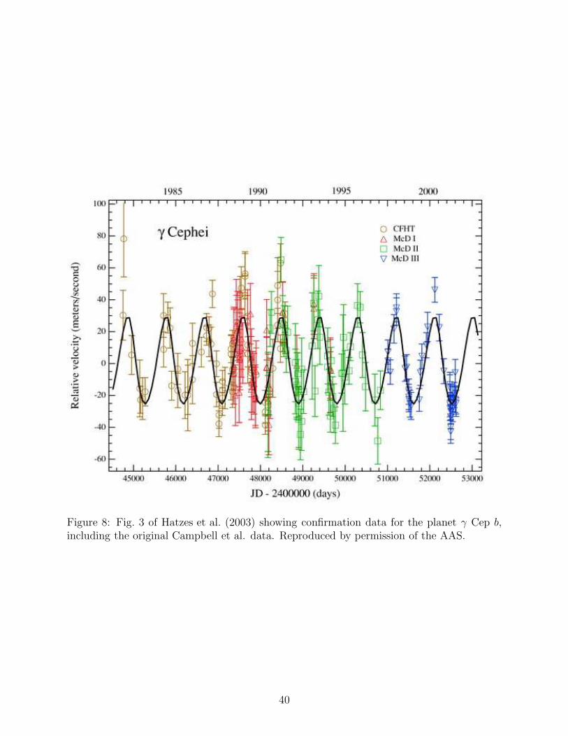
Figure 8: Fig. 3 of Hatzes et al. (2003) showing confirmation data for the planet γ Cep b,including the original Campbell et al. data. Reproduced by permission of the AAS.

40

Latham et al. sought to further stabilize their spectrograph to achieve ∼ 100 m/s precisionto measure accurate binary orbits and improve the IAU system of radial velocity standards.Latham et al. achieved this stabilization by removing the Cassegrian instrument from thetelescope, stabilizing its temperature, and feeding it with a 100-µ optical fiber. This provideda constant gravity vector, thermal and mechanical stability, and a (relatively) uniformly il-luminated entrance slit, robust against guiding errors.

On its first night of operation, Latham et al. (1989) observed several RV standard starsincluding HD 114762. They noted a large (390 m/s) radial velocity discrepancy from theknown value. Curious, they compared their previous measurements made at lower precisionand found a highly significant signal at near 84 d with 530 m/s semiamplitude, correspondingto a 13 MJup companion.

Subsequent observations at high precision confirmed the reality of the signal (see Fig. 9).Latham et al. (1989) had discovered, serendipitously, on the first night of observation, and ina sample of only seven objects, what today would be considered by many to be an exoplanet.At the time, no objects with a mass anything like 13 MJup were known, and Latham et al.cautiously referred to their object as “a probable brown dwarf”, however they noted thatthe companion “might even be a giant planet”5, a point that was picked up by the mediabut criticized by many of their colleagues (Latham 2012). Regardless of its taxonomic class,it was the first firm detection of a substellar object beyond the Solar System, and today isoften included in catalogs of exoplanets (e.g. Wright et al. 2011).

4.3.3 Marcy & Butler’s iodine survey

In 1992, Geoffrey Marcy and Paul Butler of San Francisco State University announced theirsurvey of 70 nearby stars using an iodine (I2) cell for wavelength calibration. PreviousDoppler work by Marcy & Benitz (1989) had used ThAr emission lamps to search for browndwarfs orbiting nearby M dwarfs with radial velocity precision of ∼ 250 m/s; Marcy & Butlersought to improve this precision by 1–2 orders of magnitude with their iodine cell and theCCD at the high-resolution Hamilton spectrograph, designed by Vogt (1987).

Unlike Campbell & Walker, Marcy & Butler sought an absorption cell that would provideabsorption features throughout a broad region of wavelength space. Following Libbrecht(1988) (who had employed an iodine cell to study solar sunspots and had extended theirstudies to p-mode measurements of stars) Marcy & Butler settled on iodine as the idealabsorption gas. Their rationale was that this provided the wavelength reference at everypoint in the spectrum, not just every 15A, and that the potentially problematic blending ofstellar features with iodine features could be modeled given a sufficiently accurate templatespectrum of the star and the iodine cell (the latter obtained with a Fourier TransformSpectrograph).

Marcy & Butler further sought to model the variable instrumental profile of the spectro-graph as a function of wavelength to account for the not insubstantial thermal and mechani-cal variations in the spectrograph, and for the non-uniform illumination of the entrance slit.Marcy & Butler’s sealed cell was ∼ 10 cm long, held at a constant 323 K, and 0.01 atm,

5Later, the IAU would provisionally set the deuterium-burning limit for star-like objects, 13 MJup asthe border between planets and brown dwarfs found in orbit around stars. This is useful for purposes ofnomenclature, but bears little on issues of formation and composition, and today the distinction is not alwayshonored.

41

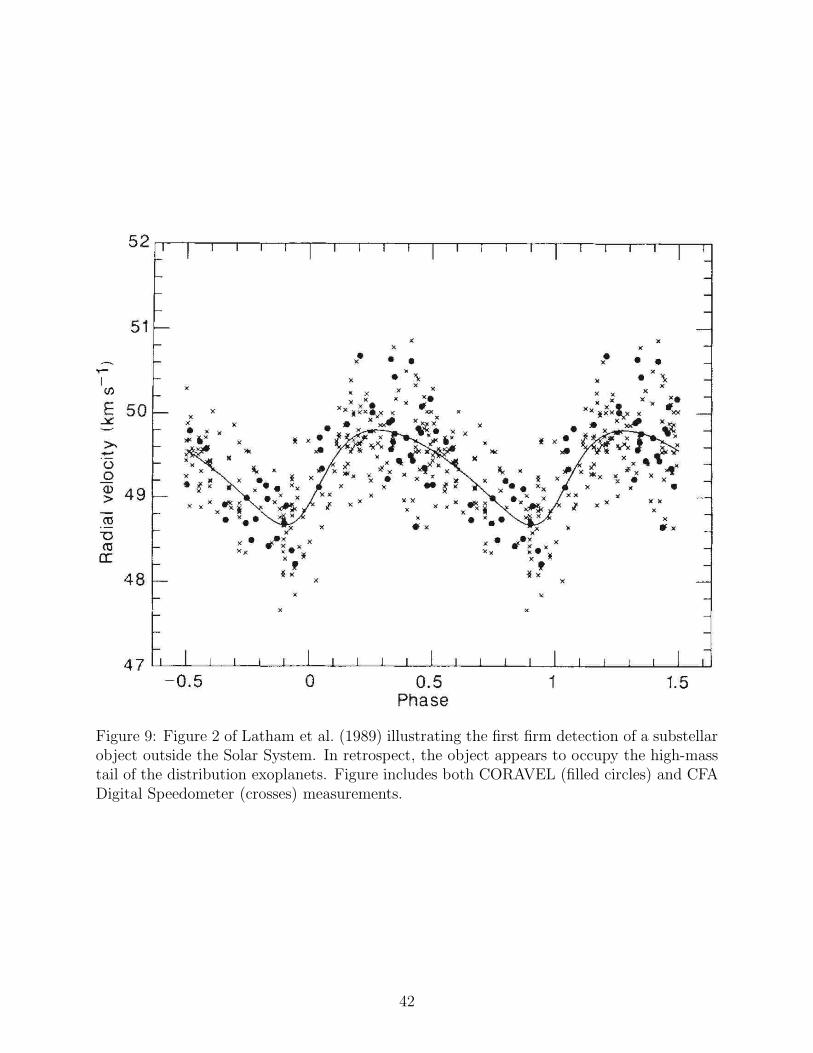
Figure 9: Figure 2 of Latham et al. (1989) illustrating the first firm detection of a substellarobject outside the Solar System. In retrospect, the object appears to occupy the high-masstail of the distribution exoplanets. Figure includes both CORAVEL (filled circles) and CFADigital Speedometer (crosses) measurements.

42

and had the further advantage that it was relatively easy to construct and its contents werebenign (indeed, medicinal!). Marcy & Butler (1992) reported that they had achieved 25m/s precision at the beginning of their survey, and foresaw significant improvement throughmore sophisticated instrumental profile modeling. Indeed, by 1996 Marcy & Butler woulddemonstrate 3 m/s precision (Butler et al. 1996) and they and their collaborators would goon to be responsible for over half of the exoplanets discovered over the next 15 years.

4.3.4 Hatzes & Cochran’s survey and β Gem b

Hatzes & Cochran (1993) reported their results from precise Doppler monitoring of threebright K giants as part of a broader planet detection effort. Their primary technique was touse telluric (atmospheric) O2 bands as an absorption wavelength reference, which had beenreported by Griffin (1973) to be sufficiently stable to allow 10 m/s precision. They foundthat typical long-term stabilities were more like 20 m/s. They had also begun employingan iodine cell (Cochran & Hatzes 1993), and at this point had obtained a small number ofiodine observations.

Hatzes & Cochran found that all three K giants in their sample, Arcturus (α Boo),Aldebaran (α Tau), and Pollux (β Gem) displayed large, periodic radial velocity variationswith semiamplitudes of 50-200 m/s. Comparison with prior radial velocities obtained byCambpell’s group (Walker et al. 1989) revealed that the variations were coherent over 10years. While both α Boo and α Tau showed significant day-to-day RV variations indicativeof radial pulsation modes and correlated variations in the 10830A He i line, β Gem seemedto have a clean signal, consistent with a 554 d planet with a minimum mass of 3 MJup.

Observations by the Canadian team (Larson et al. 1993) showed that the Ca ii 8662Aline showed periodic variation at the same frequency as the RV variations (which they hadmeasured independently). This coincidence cast strong doubt on the planetary interpretationof the β Gem RV variations, especially in light of the much larger and more clearly activity-related variations in α Boo and α Tau.

Hatzes et al. (2006) combined literature data with subsequent iodine observations fromMcDonald Observatory and Tautenburg Observatory to show that the RV variations con-tinued coherently into 2006 and that the Ca ii H & K lines showed no coincident variation.They concluded that the variations in β Gem were likely due to a minimum mass 3 MJup

companion with period 590 d.

4.3.5 Mayor & Queloz and 51 Pegasi b

The first unambiguous detection of a planet-mass object orbiting a normal star was byMayor & Queloz (1995) of Geneva Observatory. Michel Mayor and Didier Queloz used theELODIE spectrograph, which achieved 13 m/s precision through outstanding mechanicalstability. ELODIE (the successor to CORAVEL) was a fiber fed spectrograph within astable, temperature controlled environment (Queloz et al. 1998). Wavelength calibrationwas achieved through use of a simultaneous observation of a thorium-argon (ThAr) emissionlamp. Mayor & Queloz used cross-correlation with a binary mask to determine the velocityof the stellar spectrum with respect to the known wavelengths in the emission line spectrum.The mechanical stability of the instrument ensured that the offset between the stellar andcomparison lamp spectra was fixed and stable, and the scrambling inherent to the fiber

43

ensured that the position of the stellar spectrum did not suffer significantly from variationsin illumination or guiding on the fiber tip.

51 Peg b has a semiamplitude of only 59 m/s and period of only 4.2 d, implying a min-imum mass of 0.5 MJup. This was a shocking development — planet formation theory hadnot predicted the existence of such close-in planets6, and indeed the tiny mass implied bythe detection was smaller than any known binary companion by more than an order of mag-nitude.7 Immediately Marcy & Butler (1995) confirmed the detection, as did Hatzes et al.(1997) soon thereafter. Debate ensued about the nature of the variations and whether theycould be due to non-radial pulsation modes (Gray 1997), but the detection of planetary tran-sits would put these concerns to rest: the field of exoplanetary science had begun in earnest.The Geneva team would expand and find great success over the next decades, eventuallypushing their precision below 1 m/s with the HARPS spectrograph.

4.4 The First Planetary Transit: HD 209458b

The presence of close-in planets provided an opportunity to detect exoplanets directlythrough transits. The probability that a planet will transit its hosts star is inversely pro-portional to its orbital distance, and since 51 Peg b and similar “Hot Jupiters” orbited at∼ 10 stellar radii from their host stars, their transit probability was around 10%. Pho-tometrists began to monitor these planets’ hosts stars for such events, expecting to find oneonce the number of known systems approached 10. Concerns over nonradial pulsations alsocontributed to the desire to monitor stars for photometric evidence of such effects.

Two teams detected the m sin i = 0.7 MJup, P = 3.5 d planet orbiting HD 209458 in-dependently (Mazeh et al. 2000; Henry et al. 2000) and collaborated with photometrists toconduct the now-standard photometric follow-up prior to publication. Two teams succeededcontemporaneously: their announcements of the detection of the transits of HD 209458 ap-peared in the literature simultaneously, having been submitted to the Astrophysical Journalwithin one day of each other (Henry et al. 2000; Charbonneau et al. 2000) exemplifying theintense competition to produce exoplanetary “firsts”. This measurement of the orbital incli-nation and radius (and thus the true mass and density) of the planet dispelled any remainingdoubt as to the origins of most of the similar RV variations of stars, and provided the nec-essary impetus for large-scale efforts to detect more planets with radial velocities, transits,and, soon, microlensing and direct imaging.

4.5 Microlensing

4.5.1 Microlensing History

While the idea of gravitational microlensing by individual stars was considered sporadicallyover the past century (Einstein 1936; Eddington 1920; Chwolson 1924; Lodge 1919; Liebes1964; Refsdal 1964), it was the seminal paper by Paczynski (1986) that gave birth to themodern microlensing field. In this paper, Paczynski argued that it would be feasible to

6But see the remarkably prescient article by Struve (1952), which all but foresaw this detection, how itwould be made, and the subsequent detection of planetary transits.

7The third firm detection of a substellar object, the imaging of brown dwarf GJ 299 B, was announcedat the same conference as 51 Peg b!

44

monitor several million stars toward the Magellanic clouds on timescales of a few hours to afew years, in order to search for gravitational microlensing events due to foreground massivecompact objects that could make up a substantial fraction of the mass of the dark matterhalo of the Milky Way. Within a few years, several collaborations were initiated to surveyregions in the Large Magellenic Clouds and Galactic bulge to search for microlensing events(Alcock et al. 1993; Aubourg et al. 1993; Udalski et al. 1993). The first detections followedshortly thereafter, and to date of order 104 microlensing events have been detected, with themajority seen along the line of the sight to the bulge.

Although the original motivation for microlensing surveys was the search for dark matter,it was soon realized that it would be possible to search for planetary companions to the starsand remnants that provided a guaranteed signal for these experiments. Mao & Paczynski(1991) first pointed out that binary lenses whose components were separated by roughly theirEinstein ring radius would give to sharp, distinctive light curves features associated with thepresence of caustic curves in such systems. Caustics are the set of source positions where ex-tra image pairs are created or destroyed with the source crosses the caustic, resulting in largechanges in the total magnification. They also noted that the probability of a source crossingthese caustics for a binary lens remained substantial down to mass ratios of q ∼ 10−3, there-fore suggesting that planetary companions could also be detected in this way. Gould & Loeb(1992) consider this idea in detail, refining the estimates for the detection probabilities fordifferent planet mass ratios, and discussing the practical requirements for carrying out an ex-oplanet survey with microlensing. In particular, they advocated a two-tier strategy, wherebysurvey collaborations use a single dedicated telescope equipped with a wide-field cameramonitor large areas of the sky to identify and alert stellar microlensing events before peak,and follow-up collaborations with access to several longitudinally-distributed, narrow-angletelescopes follow particularly promising events at much higher cadence to search for the briefplanetary deviations. The first microlensing planet surveys began in 1995, with the first real-time alerts from the survey collaborations (e.g., Udalski et al. 1994; Alcock et al. 1996), andsubsequent monitoring of these alerts by several follow-up collaborations (Alcock et al. 1996;Albrow et al. 1998; Rhie et al. 2000).

Ongoing surveys over the next 6 years (1995-2001) failed to detect any planetary mi-crolensing events. The primary reason for this is that the total number of events alertedby the survey collaborations was relatively low (. 100), and therefore there were typicallyfew events ongoing at any given time that were both suitable for follow-up and very sen-sitive to planets. In particular, there were only a handful of high-magnification events peryear, which had been recognized to be intrinsically very sensitive to planetary companions(Griest & Safizadeh 1998). Nevertheless, this phase was important for the field, as the real-world struggles involved with carrying out and analyzing the results from these surveys,including the ensemble of non-detections (Gaudi et al. 2002; Snodgrass et al. 2004), natu-rally led to the development and maturation of both the theory and practice of the method.

4.5.2 First Planet Detections with Microlensing

The first detections of planets with microlensing were enabled primarily by a series of up-grades by several survey collaborations to their observational setups. In 2001, the OGLEcollaboration initiated their third phase with an upgrade to a new camera with a 16 timeslarger field of view. With this larger field of view, they were able to monitor a larger area

45

of the Galactic bulge with higher cadence, and as a result began alerting ∼ 500 microlens-ing events per year. This higher event rate, combined with improved cooperation betweenthe survey collaborations, led to the first planet discovery in 2003 by the Microlensing Ob-servations in Astrophysics (MOA) and OGLE collaborations (Bond et al. 2004). Shortlythereafter, the MOA collaboration upgraded to a 1.8m telescope with a 2 deg2 camera(Sako et al. 2008). By 2007, the MOA and OGLE collaborations were sending alerts fornearly 1000 microlensing events per year, thus enabling a substantial increase in the rate ofplanet detections.

The light curve data and best-fit model for the first microlensing planet discovery areshown in Figure 10. This is a “cold Jupiter”: the planet has a mass Mp ∼ 3 MJup and orbitsa star with M∗ ≃ 0.6 M⊙ at a separation of a ∼ 4AU, or ∼ 2.5 times the snow line distance(Bennett et al. 2006).

To date, 14 microlensing planet detections have been published. The masses and semi-major axes of these planets are shown in Figure 5, they span nearly three decades in massfrom a few times the mass of the Earth to several times the mass of Jupiter, and are spreadover a factor of ∼ 5 in separation, centered at a few times the snow line distance. Notableamong these detections are the first discovery of a “cold SuperEarth” (Beaulieu et al. 2006),and the first discovery Jupiter/Saturn analog (Gaudi et al. 2008; Bennett et al. 2010a).

5 State of the Art

5.1 Astrometry

Astrometric precision has improved considerably since van de Kamp’s work, and the firstverifiable astrometric discovery of an exoplanet appears imminent. Pravdo & Shaklan (2009)announced that their long-term astrometric monitoring of the ultra-cool dwarf star vB 10 hadrevealed a ∼ 6MJup companion in a 9 month orbit, however subsequent followup with radialvelocities determined that the signal was spurious (Bean et al. 2010; Anglada-Escude et al.2010; Lazorenko et al. 2011).

More promisingly, Muterspaugh et al. (2010) used an optical interferometer to carefullymeasure the astrometric motions of binary stars, and combined these measurements withradial velocities of the systems to search for low mass companions to stars in tight bina-ries. The project concluded with six planetary candidates, including two “high confidence”members that could prove to be the first astrometrically detected exoplanets. If real, theseplanets will put strong constraints on planet formation theories in binary systems.

The astrometric detection of planets discovered by other means has produced substan-tially more results, primarily because the approximate astrometric signals are known fromprior radial velocity work and so searches are more efficient. Most fruitful has been work onnearby stars employing the Hubble Space Telescope Fine Guidance Sensor, which is capableof precise astrometry of bright stars. This has revealed some high-mass planet candidatesfrom radial velocity surveys to be binary stars in face-on orbits, and has revealed the mu-tual inclinations of planets in multiplanet systems (Bean et al. 2007; Bean & Seifahrt 2009;McArthur et al. 2010).

46

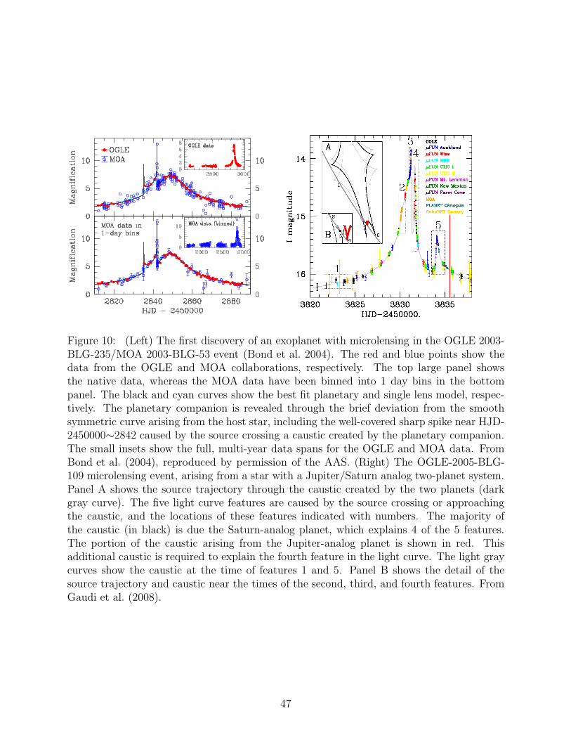
Figure 10: (Left) The first discovery of an exoplanet with microlensing in the OGLE 2003-BLG-235/MOA 2003-BLG-53 event (Bond et al. 2004). The red and blue points show thedata from the OGLE and MOA collaborations, respectively. The top large panel showsthe native data, whereas the MOA data have been binned into 1 day bins in the bottompanel. The black and cyan curves show the best fit planetary and single lens model, respec-tively. The planetary companion is revealed through the brief deviation from the smoothsymmetric curve arising from the host star, including the well-covered sharp spike near HJD-2450000∼2842 caused by the source crossing a caustic created by the planetary companion.The small insets show the full, multi-year data spans for the OGLE and MOA data. FromBond et al. (2004), reproduced by permission of the AAS. (Right) The OGLE-2005-BLG-109 microlensing event, arising from a star with a Jupiter/Saturn analog two-planet system.Panel A shows the source trajectory through the caustic created by the two planets (darkgray curve). The five light curve features are caused by the source crossing or approachingthe caustic, and the locations of these features indicated with numbers. The majority ofthe caustic (in black) is due the Saturn-analog planet, which explains 4 of the 5 features.The portion of the caustic arising from the Jupiter-analog planet is shown in red. Thisadditional caustic is required to explain the fourth feature in the light curve. The light graycurves show the caustic at the time of features 1 and 5. Panel B shows the detail of thesource trajectory and caustic near the times of the second, third, and fourth features. FromGaudi et al. (2008).

47

5.2 Imaging

5.2.1 2M1207b

Chauvin et al. (2010) describe their survey of young, nearby stars for low mass, possiblyplanetary companions using the ESO/VLT 8-m telescope equipped with the NACO AOsystem and infrared camera. They began their survey in 2002 during commissioning, andtargeted, among other things, the lowest mass members of known, nearby, young stellarassociations. This allowed them to maximize the separation and contrast of companions andpush coronagraphy into the planetary-mass regime.

After some promising detections of higher mass objects, the survey bore fruit whenChauvin et al. (2004) detected a very low mass companion to the M8 TW Hydra association(TWA) brown dwarf 2MASSW J1207334-393254 (called 2M1207; Figure 11) at a separa-tion of only 0.′′8 (∼ 55 AU). Membership in the TWA yielded an age for the companion,and a distance was estimated from the colors and brightness of 2M1207. Comparison withmodels of the thermal evolution of young objects (Burrows et al. 1997; Chabrier et al. 2000;Baraffe et al. 2002) allowed Chauvin et al. (2004) to estimate the companions mass to be∼ 5 MJup, assuming that it was indeed a bound, coeval object and not a background con-taminant.

Chauvin et al. (2005) followed up their prior observations to confirm common propermotion using the same instrument. They demonstrated that the two objects share propermotion and parallactic motion with this star, all but proving that they form a bound pair.

The nature of 2M1270b was, and still is, unclear. Its status as a “planetary-mass” objectseems secure, but its wide separation (55 AU) and ∼0.2 mass ratio with its primary madethe pair perhaps more analogous to a scaled-down binary star system than a planet-starsystem. Chauvin et al. (2005) noted that a protoplanetary disk origin for the b componentseemed unlikely. Nonetheless, they had acquired the first image of a planet, by mass if not byformation mechanism, and this presaged the many more successes to come from high contrastimaging. The ESO/VLT group would go on to detect the planet-mass object AB Pic b andmany faint stellar companions to nearby stars, including many planet hosts (Chauvin et al.2010).

5.2.2 Fomalhaut b

Kalas et al. (2005) used the Hubble Space Telescope (HST) Advanced Camera for Surveys(ACS) to image the dust belt orbiting Fomalhaut (α Piscis Austrini), a ∼400 Myr-old A4dwarf at 7.7 pc. Debris disks or belts are a common feature of many young main sequencestars, typically with structure consistent with dynamical interactions from unseen planets(see chapter by Moro-Martin). The coronagraphic mode of ACS allowed the HST teamto make a spectacular and detailed image of the disk in reflected optical light, revealingthat its dominant feature is a highly inclined, off-center belt with an apparently sharp inneredge at 133 AU radius. The 15 AU geometric offset of the belt from the star and thesharp inner edge could be explained by the presence of a planetary companion with non-zeroeccentricity “sculpting” the inner edge of the belt and maintaining the geometric offset viasecular perturbation (Wyatt et al. 1999).

Follow-up observations to determine the structure of the disk using a variety of PSFsubtraction techniques allowed Kalas et al. (2008) to confirm a persistent source with optical

48

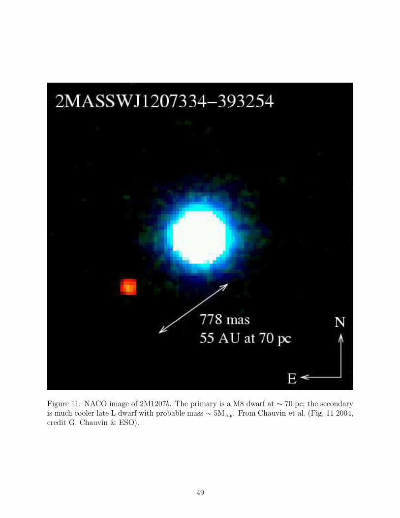
Figure 11: NACO image of 2M1207b. The primary is a M8 dwarf at ∼ 70 pc; the secondaryis much cooler late L dwarf with probable mass ∼ 5MJup. From Chauvin et al. (Fig. 11 2004,credit G. Chauvin & ESO).

49

brightness ∼ 25 mag and located ∼13′′ away from the primary star, just inside the belt, andconsistent with the “sculpting” hypothesis. Comparison of multiple epochs allowed Kalas’steam to measure the orbital motion of the object astrometrically and confirm that it is aproper motion companion of Fomalhaut.

Puzzlingly, this very faint companion did not appear in their infrared imaging at theKeck 10-m and Gemini 8-m telescopes, which is inconsistent with the optical emission beingthermal in origin according to current models. Kalas et al. were able to use the dust diskitself to constrain the object’s mass dynamically to be < 3MJup (Chiang et al. 2009), andthus the lowest mass directly imaged planet candidate to date. Kalas et al. (2008) proposedseveral possible explanations for Fomalhaut b’s unusual optical brightness, such as reflectionfrom a circumplanetary dust ring that could be as large as 35 planetary radii, though stillsignificantly smaller than Saturn’s Phoebe ring. They also proposed an alternative modelwhere reflected light is due to a transient dust cloud produced by a rare destructive collisionbetween two analogs of solar system Kuiper Belt objects.

As with 2M1207b, ascertaining the nature of Fomalhaut b will require additional observa-tions and theoretical input. It orbits an intermediate mass star with semi-major axis ∼ 120AU, and is still undetected in the infrared. Whatever its nature, its presence in a disk ofmaterial strongly implicates a disk origin for the object, and provides hope for more securesimilar detections of similarly bright planetary objects in the future.

5.2.3 Beta Pictoris b

β Pic is an A star with a prominent, edge-on debris disk that was the first to be imaged inoptical scattered light (Smith & Terrile 1984). One unexpected result was that the disk hadseveral asymmetries in structure (Kalas & Jewitt 1995), including a vertical warp in the diskmidplane at <100 AU projected radius from the star (Burrows et al. 1995). These and otherphenomenon observed toward β Pic indirectly suggested the existence of a planetary system,and β Pic b was finally directly imaged using VLT/NACO (Lagrange et al. 2009). As withFomalhaut, the debris disk structure could be used to constrain the planet mass throughdynamical theory (Mouillet et al. 1997), as an alternative to mass estimates based on planetluminosity models. Its measured L′ brightness of 11th mag corresponds to a ∼ 8 MJup planetat age ∼10 Myr.

β Pic b is currently unique among the directly imaged exoplanets for having the smallestsemi-major axis, which, at ∼8 AU, corresponds to the approximate ice-line of the system.Unfortunately, the projected separation is also very small, 0.′′4, and follow-up spectroscopicstudy has yet to be obtained. Systems such as β Pic are therefore ideal targets for the nextgeneration of extreme adaptive optics instrumentation discussed below. These future resultswill provide important tests of various planet formation and luminosity evolution models,which in the 10 Myr-age regime offer significantly different predictions for the physical prop-erties of Jupiter-mass planets.

5.2.4 The HR 8799 Planetary System

A US/Canadian team led by Marois used AO coronagraphy on the Keck and Gemini tele-scopes in angular differential imaging mode (ADI, Marois et al. 2006), which exploits therotation of the field of view on an altitude/azimuth telescope with time to distinguish (and

50

subtract) PSF features from astrophysical sources. Marois’ team observed the nearby (40pc) A star HR 8799, which was known to have an IR excess and to be relatively young (20–160 Myr), making any orbiting planets likely to be bright in the near infrared. Marois et al.(2008) reported the discovery of three faint companions to HR 8799, with proper motionsconsistent with HR 8799 and detectable orbital motion. Comparison with Pleiades browndwarf brightnesses demonstrated that these objects had likely masses below 11 MJup. Fur-ther observations at Keck Observatory allowed Marois et al. (2010) to discover a fourth, ecomponent to the system. The projected orbital separations of the four planets range from14–70 AU.

This family of objects, the first imaged multi-planet system, poses special challengesfor planet formation theory. Marois et al. (2010) argue that their masses and orbital radii(and the relative scarcity of other systems such as this) are inconsistent with both in situgravitational-instability disk fragmentation and core-accretion scenarios. Like the close-in“hot Jupiters”, these distant planets would seem to implicate migration in a disk as a primaryarchitectural factor in planetary system formation.

5.2.5 SPHERE, GPI, and Project 1640

Several “extreme” adaptive optics systems with coronagraphs are in development or oper-ation, and will be capable of detecting young (< 1 Gyr) giant planets at a few diffractionwidths from the position of a bright star. Such systems employ deformable mirrors withseveral hundreds to thousands of actuators, and typically observe bright stars in the nearinfrared. They use integral field spectrographs produce data cubes (i.e. a low resolutionspectrum at each angular position) and can exploit field rotation to employ a variety of PSFsubtraction and speckle suppression techniques. They thus produce large data volumes, in-cluding spectra of their imaged planets, and will typically have narrow fully-corrected fieldsof view (< 1′′).

Project 1640 (Hinkley et al. 2011), already in operation, is a collaboration between theAmerican Museum of Natural History and the University of Cambridge. It employs thePALM 3000 adaptive optics system on the Hale 200-in telescope at Palomar Observatory.SPHERE (Beuzit et al. 2006) and GPI (Macintosh et al. 2008) are next-generation corona-graphic imagers on the VLT and Gemini South telescopes, respectively. Both will employthousands of actuators and execute campaigns to discover young Jupiter-mass planets or-biting at several AU from the nearest Sun-like stars. Depending on the adopted planetformation and luminosity evolution model, the detection rate predicted for GPI ranges be-tween 10% and 25%, given a target sample with age <100 Myr within 75 pc (McBride et al.2011). Therefore, if these instruments observe ∼500 stars from this sample, then there willbe at least 50 new exoplanets discovered and characterized via direct imaging.

5.3 Rocky and Habitable Worlds

5.3.1 HARPS, Keck/HIRES, and the Planet Finding Spectrograph

The first RV-discovered planets had typical Doppler amplitudes of ∼ 50–500 m/s; the 10 m/sbarrier was breached several times between 2000-2005, and detections between 2–5 m/s werecommon between 2005-2010. The primary instruments making these detections were the

51

HIRES instrument on the Keck i telescope (operated by various teams of Marcy & Butler)with precision as low as 1–3 m/s, and the HARPS spectrograph (with its heritage fromthe Geneva team) which regularly achieves precision below 1 m/s on bright stars. Severalnext generation planet finding spectrographs are being built or commissioned at this writing,including the Planet Finding Spectrograph at Magellan, HARPS-North, and ESPRESSO.

There are two primary obstacles to further precision in radial velocity surveys towardsthe 10 cm/s necessary for the detection of true Earth analogs. The first is an instrumentalstability issue: calibrating the wavelength solution of spectrographs to an order of magnitudebetter precision than previously possible. For emission-lamp calibration, a fundamental limitis the lifetime and stability of the thorium-argon lamps used as wavelength fiducial. Apromising solution is the use of laser frequency combs, which provide essentially arbitrarylevels of wavelength precision. Such devices will be used in HARPS-North and ESPRESSO.Also of importance is understanding and maximizing the consistency of the illumination ofthe output fibers used to guide light to the spectrograph.

For absorption-cell instruments, the practical limit is one’s ability to model the system,in particular the absorption cell, the slit illumination function, the instrumental profile, andthe star itself. Progress here is primarily made through careful FTS scans of the actual cellused at the telescope, improved modeling techniques that account for scattered light, andbetter deconvolution techniques for acquiring stellar templates.

The second obstacle is that of the fundamental stability of the stars themselves. Starsexperience p-mode oscillations at the few m/s level that must be either modeled or aver-aged over. Stellar magnetic surface activity also contributes to radial velocity signatures inmany ways, most importantly through rotationally modulated spots and plage, and perhapsthrough long-term stellar cycles. Modeling and mitigating these effects, perhaps thoughcareful use of contemporaneous photometry, will be necessary to achieve the next large im-provement in RV precision for the next generation of planet searches.

5.3.2 Space-Based Transit Surveys

Transit surveys for rocky planets around solar-type stars require extremely precise relativephotometry. The fractional depth of the transit of an Earth-sized planet passing in front of asolar radius star is only δ ∼ 8×10−5. While relative photometry at a few times this level hasbeen achieved from the ground for individual bright stars with specialized techniques (e.g.,Johnson et al. 2009; Southworth et al. 2009; Colon et al. 2010), obtaining . 10−4 relativephotometry for the large ensembles of stars required to detect numerous transiting systems isprobably out of reach for ground-based surveys, due to unavoidable systematics arising fromvariations due to the Earth’s atmosphere. The stability afforded by space-based surveys,on the other hand, enables relative photometry for large numbers of stars that is limitedprimarily by photon and astrophysical noise. Furthermore, for space-based surveys it ispossible to obtain continuous photometry for very long periods of time, without diurnal orweather interruptions. This eliminates the aliasing problems that are germane to single-siteground-based transit surveys, and enables the detection of long period transiting systems,which, due to the low duty cycles and long transit durations, are extremely difficult to detectfrom the ground .

CoRoT is a CNES-led space mission with participation from ESA and other internationalpartners, with the primary goals of studying stars via asteroseismology and detecting tran-

52

siting planets (Baglin 2003). The 27cm telescope was launched in December 2006, and islocated in a Low Earth Orbit. CoRoT is equipped with a 3.05 by 2.7 camera that pri-marily monitors fields in two different areas of the sky, located toward Galactic longitudesof ∼ 40 and ∼ 210 (Auvergne et al. 2009). There are two dwell times for the fields; longfields are typically observed for ∼ 150 days, whereas short fields are observed for ∼ 30 days.To date more than 130,000 stars in ∼ 20 fields have been monitored with a cadence of 8.5minutes (Michel & Baglin 2012). The stellar populations of these fields vary dramatically,but anywhere from 40−60% of the targets are expected to be dwarf stars suitable for transitsurveys (Cabrera et al. 2009; Erikson et al. 2012). Over the typical R ∼ 12− 16 magnituderange of the targets, CoRoT achieves relative photometry on time scales of ∼ 2 hours atthe level of ∼ 10−4 at the bright end, degrading to ∼ 10−3 at R ∼ 16 (Aigrain et al. 2009).The precision and cadence is sufficient to detect Jupiter-sized companions over the entiremagnitude range, whereas Neptunes and Super-Earths can be detected around the brighterstars (e.g., Cabrera et al. 2009).

To date, CoRoT has announced over 20 detections of transiting planets and brown dwarfs.Notable among these discoveries are the detection of a transiting brown dwarf with a mass of∼ 60 MJup (Bouchy et al. 2011), the detection of a Jupiter-sized planet with a relatively longperiod of ∼ 95 days (Deeg et al. 2010), and the first detection of a transiting Super-Earth,with a radius of ∼ 1.7R⊕ and a mass of 3− 10 M⊕ (Leger et al. 2009).

Kepler is a NASA mission launched in March of 2009, with the primary goal of mea-suring the frequency of rocky planets in the Habitable Zones of sunlike stars (Borucki et al.2010). To accomplish this, the 0.95m Kepler telescope situated in an Earth-trailing orbitis monitoring a 105 square degree field-of-view near the constellation Cygnus continuouslyover the 7+ year lifetime of the mission. Light curves of ∼ 200, 000 stars have been ob-tained over the course of the mission, with typical sampling cadences of ∼ 30 minutes,amounting to ∼ 24, 000 observations over the first ∼ 500 days of the mission for the subsetof stars monitored continuously during this time (Batalha et al. 2012). A subset of starshave higher cadences of ∼ 1 minute. The majority of the target stars are solar-type dwarfswith Teff ∼ 5000 − 6500 K and log g ∼ 4.5, but the full range of target properties spanTeff ≃ 3500 − 10, 000 K and log g ≃ 3 − 5 (Batalha et al. 2012). The photometric precisionand intrinsic stellar variability of this sample is discussed in Gilliland et al. (2011). Relevantto the primary mission goal, the photometric variability for V . 12 stars on transit timescales is ∼ 3×10−5, quite an impressive figure, but ∼ 50% larger than originally anticipated,primarily due to the fact that typical target stars turn out to be a factor of ∼ 2 times morevariable than the Sun, probably due to their relative youth. Although this increased noisereduces the expected sensitivity and so yield of the mission for habitable Earthlike planets,this reduced sensitivity was offset with a mission extension (Gilliland et al. 2011).

Although the data set is not yet sufficient to reliably detect true Earth analogs, theexquisite photometric precision and large sample size has already enabled an fantastic arrayof science. In particular, based on the first ∼ 500 days of data, a total of ∼ 2, 300 transitingplanets candidates have been identified (Batalha et al. 2012), including ∼ 360 multi-planetsystems (Fabrycky et al. 2012). The majority of these candidates are smaller than Neptune.Despite the fact that a small fraction of these signals have been confirmed by either radial ve-locity or transiting timing methods, the overwhelming majority of these signals are expectedto be due to real planets, from a number of lines of evidence (e.g., Morton & Johnson 2011;Lissauer et al. 2012). Over 30 systems have been confirmed from various methods, including

53

a system with six transiting planets (Lissauer et al. 2011), the first discovery of a circumbi-nary planet (Doyle et al. 2011), and several planets with radius of . R⊕ (Muirhead et al.2012; Fressin et al. 2012).

The masses and semimajor axes of the confirmed CoRoT and Kepler systems with massmeasurements as of Dec. 2011 are shown in Figure 5. Comparing these to the planetsdiscovered by ground-based transit surveys highlights the large expansion of discovery spacethat is enabled by going to space.

5.3.3 Second Generation Microlensing Surveys

Microlensing exoplanet searches are currently in the midst of a transition to the secondgeneration of surveys that will enable the routine detection of rocky planets. Althoughthere have been substantial modifications and upgrades to the details of the “two-tier”survey strategy initially suggested by Gould & Loeb (1992), up until very recently this basicapproach has been in use. Second generation surveys will operate in a very different manner.With the development of very large format CCD cameras with fields of view of a squaredegree or greater, it becomes possible to monitor tens of square degrees of the Galacticbulge containing roughly 100 million stars with cadences of tens of minutes. These cadencesare sufficient to detect both the primary event and detect the perturbations from low-mass(∼ M⊕) planets, therefore obviating the need for a follow-up observations and allowing formore uniform data and a more objective detection criteria. In order to detect all the planetaryperturbations, including those that last less than a day, a longitudinally-distributed networkof 1− 2m class telescopes equipped with such wide FOV cameras is required.

The transition to the next generation survey model began in 2006 when MOA upgradedto the dedicated MOA-II telescope in New Zealand, which has a diameter of 1.8m and 2.2deg2 FOV (Sako et al. 2008; Hearnshaw et al. 2006). In 2010, OGLE upgraded to the 1.4deg2 OGLE-IV camera on their dedicated 1.3m telescope in Chile (Udalski 2009). TheWise Observatory 1.0m telescope in Israel recently been equipped with a 1 deg2 camera(Gorbikov et al. 2010). These three groups are collaborating to continuously monitor an ∼ 8deg2 region of the bulge with cadences of 15-30 minutes (Shvartzvald & Maoz 2012), and thefirst planet detection with this strategy was recently announced (Yee et al. 2012).

The next milestone in the development of second generation microlensing surveys willbe the completion of the Korean Microlensing Telescope Network (KMTNet). KMTNet isan ambitious, fully funded plan by the Korean government to build three identical 1.6mtelescopes with 4 deg2 FOV cameras. These will be located in South America, South Africa,and Australia. First light for the final telescope is scheduled for late 2014.

These second generation surveys are expected in increase the planet yields by roughlyan order of magnitude over current surveys (Bennett 2004; Shvartzvald & Maoz 2012), andenable the detection of Earth-mass planets, as well as free-floating planets with massesgreater than ∼ 10 M⊕.

6 Conclusions

In the roughly two decades since the first detections of planets outside the solar system,the field of exoplanets has grown enormously, developing into one of the forefront research

54

areas in astronomy. The count of confirmed planets is now over 700, with the sampledoubling in size every few years at the current rate. New techniques, methods, experiments,instruments, telescopes and satellites to detect exoplanets are constantly being developed,and are enabling the detection and characterization of an increasingly broad diversity ofplanets orbiting a wider and wider range of hosts. These efforts are not only continuallyuncovering new and unexpected types of planetary systems, but are beginning to allow forthe robust statistical characterization of the demographics of large samples of exoplanetsspanning a wide range of parameter space. These efforts ultimately serve to allow us achievethe more general goals of placing our solar system in the context of planetary systemsthrough the Galaxy, understanding the physics of planetary formation and evolution, anddetermining the frequency of habitable and inhabited worlds.

ACKNOWLEDGMENTS

B.S.G. would like to thank Thomas Beatty and Karen Mogren for permission to discussresults in advance of submission, and acknowledges support from NSF CAREER GrantAST-1056524.

J.T.W. acknowledges support by funding from the Center for Exoplanets and HabitableWorlds. The Center for Exoplanets and Habitable Worlds is supported by the Pennsyl-vania State University, the Eberly College of Science, and the Pennsylvania Space GrantConsortium.

This work makes extensive use of NASA’s Astrophysics Data System, the ExoplanetOrbit Database at exoplanets.org, and the Extrasolar Planets Encyclopedia at exoplanet.eu.

References

Aigrain, S., Pont, F., Fressin, F., et al. 2009, A&A, 506, 425Agol, E., Steffen, J., Sari, R., & Clarkson, W. 2005, MNRAS, 359, 567Agol, E. 2007, MNRAS, 374, 1271Albrow, M., Beaulieu, J.-P., Birch, P., et al. 1998, ApJ, 509, 687Alcock, C., Akerlof, C. W., Allsman, R. A., et al. 1993, Nature, 365, 621Alcock, C., Allsman, R. A., Alves, D., et al. 1996, ApJ, 463, L67Anglada-Escude, G., Shkolnik, E. L., Weinerger, A. J., Thompson, I. B., Osip, D. J., &Debes, J. H. 2010, ApJ, 711, L24

Applegate, J. H. 1992, ApJ, 385, 621–629Aubourg, E., Bareyre, P., Brehin, S., et al. 1993, Nature, 365, 623Auvergne, M., Bodin, P., Boisnard, L., et al. 2009, A&A, 506, 411Baglin, A. 2003, Advances in Space Research, 31, 345Bailes, M., Lyne, A. G., & Shemar, S. L. 1991, Nature, 352, 311Bailes, M., Bates, S. D., Bhalerao, V., et al. 2011, Science, 333, 1717Bakos, G., Noyes, R. W., Kovacs, G., et al. 2004, PASP, 116, 266Batalha, N. M., Rowe, J. F., Bryson, S. T., et al. 2012, arXiv:1202.5852Ballard, S., Fabrycky, D., Fressin, F., et al. 2011, ApJ, 743, 200Baraffe, I., Chabrier, G., Allard, F., & Hauschildt, P. H. 2002, A&A, 382, 563

55

Bean, J. L., McArthur, B. E., Benedict, G. F., et al. 2007, AJ, 134, 749Bean, J. L., & Seifahrt, A. 2009, A&A, 496, 249Bean, J. L., Seifahrt, A., Hartman, H., Nilsson, H., Reiners, A., Dreizler, S., Henry, T. J.,& Wiedemann, G. 2010, ApJ, 711, L19

Bean, J. L., Seifahrt, A., Hartman, H., et al. 2010, ApJ, 713, 410Beaulieu, J.-P., Bennett, D. P., Fouque, P., et al. 2006, Nature, 439, 437Bennett, D. P. 2004, Extrasolar Planets: Today and Tomorrow, 321, 59Bennett, D. P. 2008, Exoplanets: Detection, Formation, Properties, Habitability, ed. J. Ma-son (Berlin, Springer) 47-88

Bennett, D. P., & Rhie, S. H. 1996, ApJ, 472, 660Bennett, D. P., & Rhie, S. H. 2002, ApJ, 574, 985Bennett, D. P., Anderson, J., Bond, I. A., Udalski, A., & Gould, A. 2006, ApJ, 647, L171Bennett, D. P., Anderson, J., & Gaudi, B. S. 2007, ApJ, 660, 781Bennett, D. P., Rhie, S. H., Nikolaev, S., et al. 2010a, ApJ, 713, 837Bennett, D. P., Anderson, J., Beaulieu, J. P., et al. 2010b, arXiv:1012.4486Beuzit, J.-L., Feldt, M., Dohlen, K., et al. 2006, The Messenger, 125, 29Blake, C. H., Bloom, J. S., Latham, D. W., et al. 2008, PASP, 120, 860Bond, I. A., Udalski, A., Jaroszynski, M., et al. 2004, ApJ, 606, L155Borucki, W. J., Koch, D., Basri, G., et al. 2010, Science, 327, 977Bouchy, F., Deleuil, M., Guillot, T., et al. 2011, A&A, 525, A68Brown, R. A. 2005, ApJ, 624, 1010Burrows, C. J., Krist, J. E., Stapelfeldt, K. R., and the WFPC2 Investigation DefinitionTeam 1995, BAAS, 187.3205

Burrows, A., Marley, M., Hubbard, W. B., et al. 1997, ApJ, 491, 856Butler, R. P., Marcy, G. W., Williams, E., McCarthy, C., Dosanjh, P., & Vogt, S. S. 1996,PASP, 108, 500

Cabrera, J., Fridlund, M., Ollivier, M., et al. 2009, A&A, 506, 501Campbell, B., Walker, G. A. H., & Yang, S. 1988, ApJ, 331, 902Chabrier, G., Baraffe, I., Allard, F., & Hauschildt, P. 2000, ApJ, 542, 464Charbonneau, D., Brown, T. M., Latham, D. W., & Mayor, M. 2000, ApJ, 529, L45Charbonneau, D., Berta, Z. K., Irwin, J., et al. 2009, Nature, 462, 891Chauvin, G., Lagrange, A.-M., Dumas, C., Zuckerman, B., Mouillet, D., Song, I., Beuzit,J.-L., & Lowrance, P. 2004, A&A, 425, L29

—. 2005, A&A, 438, L25Chauvin, G., et al. 2010, A&A, 509, A52+Chiang, E., Kite, E., Kalas, P., Graham, J. R., & Clampin, M. 2009, ApJ, 693, 734Chwolson, O. 1924, Astronomische Nachrichten, 221, 329Colon, K. D., Ford, E. B., Lee, B., Mahadevan, S., & Blake, C. H. 2010, MNRAS, 408, 1494Cochran, W. D., & Hatzes, A. P. 1993, in Astronomical Society of the Pacific ConferenceSeries, Vol. 36, Planets Around Pulsars, ed. J. A. Phillips, S. E. Thorsett, & S. R. Kulkarni,(San Francisco, CA: ASP), 267–273

Cumming, A. 2004, MNRAS, 354, 1165Deeg, H. J., Moutou, C., Erikson, A., et al. 2010, Nature, 464, 384Deming, D., Seager, S., Winn, J., et al. 2009, PASP, 121, 952Di Stefano, R., & Night, C. 2008, arXiv:0801.1510Dominik, M., Jørgensen, U. G., Rattenbury, N. J., et al. 2010, Astronomische Nachrichten,

56

331, 671Doyle, L. R., Carter, J. A., Fabrycky, D. C., et al. 2011, Science, 333, 1602Eddington, A. S. 1920, Cambridge Science Classics, Cambridge: University Press, 134Einstein, A. 1936, Science, 84, 506Eisner, J. A., & Kulkarni, S. R. 2001, ApJ, 550, 871Erikson, A., Santerne, A., Renner, S., et al. 2012, A&A, 539, A14Erskine, D. J., & Ge, J. 2000, in Astronomical Society of the Pacific Conference Series, Vol.195, Imaging the Universe in Three Dimensions, ed. W. van Breugel & J. Bland-Hawthorn,(San Francisco, CA: ASP), 501–+

Fabrycky, D. C., Lissauer, J. J., Ragozzine, D., et al. 2012, arXiv:1202.6328Ford, E. B., Ragozzine, D., Rowe, J. F., et al. 2012, arXiv:1201.1892Fressin, F., Torres, G., Rowe, J. F., et al. 2012, Nature, 482, 195Gaudi, B. S., Albrow, M. D., An, J., et al. 2002, ApJ, 566, 463Gaudi, B. S., Bennett, D. P., Udalski, A., et al. 2008, Science, 319, 927Gaudi, B. S. 2010, in Exoplanets, ed. S. Seager (Tucson:University of Arizona Press), p79Gaudi, B. S. 2012, ARA&A, 50, 411Gilliland, R. L., Chaplin, W. J., Dunham, E. W., et al. 2011, ApJS, 197, 6Gorbikov, E., Brosch, N., & Afonso, C. 2010, Ap&SS, 326, 203Gould, A. 2000, ApJ, 535, 928Gould, A., & Gaucherel, C. 1997, ApJ, 477, 580Gould, A., Loeb, A. 1992, ApJ, 396, 104Gould, A., Ford, E. B., & Fischer, D. A. 2003a, ApJ, 591, L155Gould, A., Pepper, J., & DePoy, D. L. 2003b, ApJ, 594, 533Gould, A., Dorsher, S., Gaudi, B. S., & Udalski, A. 2006, Acta Astron., 56, 1Gould, A., Dong, S., Gaudi, B. S., et al. 2010, ApJ, 720, 1073Gray, D. F. 1997, Nature, 385, 795Green, J., Schechter, P., Baltay, C., et al. 2011, arXiv:1108.1374Griest, K., & Safizadeh, N. 1998, ApJ, 500, 37Griffin, R. 1973, MNRAS, 162, 243Hatzes, A. P., & Cochran, W. D. 1993, ApJ, 413, 339Hatzes, A. P., Cochran, W. D., Endl, M., McArthur, B., Paulson, D. B., Walker, G. A. H.,Campbell, B., & Yang, S. 2003, ApJ, 599, 1383

Hatzes, A. P., Cochran, W. D., & Johns-Krull, C. M. 1997, ApJ, 478, 374Hatzes, A. P., Cochran, W. D., Endl, M., et al. 2006, A&A, 457, 335Hearnshaw, J. B., Abe, F., Bond, I. A., et al. 2006, The 9th Asian-Pacific Regional IAUMeeting, (Indonesia, Bali: Nusa Dua), 272

Henry, G. W., Marcy, G. W., Butler, R. P., & Vogt, S. S. 2000, ApJ, 529, L41Hinkley, S., Oppenheimer, B. R., Zimmerman, N., et al. 2011, PASP, 123, 74Holman, M. J., & Murray, N. W. 2005, Science, 307, 1288Holtzman, J. A., Watson, A. M., Baum, W. A., et al. 1998, AJ, 115, 1946Horne, K., Snodgrass, C., & Tsapras, Y. 2009, MNRAS, 396, 2087Ida, S., & Lin, D. N. C. 2004, ApJ, 604, 388Johnson, J. A., Winn, J. N., Cabrera, N. E., & Carter, J. A. 2009, ApJ, 692, L100Kalas, P. & Jewitt, D. 1995, AJ, 110, 794Kalas, P., Graham, J. R., & Clampin, M. 2005, Nature, 435, 1067Kalas, P., et al. 2008, Science, 322, 1345

57

Kane, S. R., Mahadevan, S., von Braun, K., Laughlin, G., & Ciardi, D. R. 2009, PASP, 121,1386

Kasdin, N. J., Vanderbei, R. J., Spergel, D. N., & Littman, M. G. 2003, ApJ, 582, 1147Kasting, J. F., Whitmire, D. P., & Reynolds, R. T. 1993, Icarus, 101, 108–128Kennedy, G. M., & Kenyon, S. J. 2008, ApJ, 673, 502Kiraga, M., & Paczynski, B. 1994, ApJ, 430, L101Lagrange, A.-M., Gratadour, D., Chauvin, G., et al. 2009, A&A, 493, L21Larson, A. M., Irwin, A. W., Yang, S. L. S., Goodenough, C., Walker, G. A. H., Walker,A. R., & Bohlender, D. A. 1993, PASP, 105, 825

Latham, D. W., Stefanik, R. P., Mazeh, T., Mayor, M., & Burki, G. 1989, Nature, 339, 38Latham, D. W. 2012, New A Rev., 56, 16Lazorenko, P. F., et al. 2011, A&A, 527, A25+Leger, A., Rouan, D., Schneider, J., et al. 2009, A&A, 506, 287Libbrecht, K. G. 1988, ApJ, 330, L51Liebes, S. 1964, Physical Review, 133, 835Lissauer, J. J. 1987, Icarus, 69, 249Lissauer, J. J., Fabrycky, D. C., Ford, E. B., et al. 2011, Nature, 470, 53Lissauer, J. J., Marcy, G. W., Rowe, J. F., et al. 2012, arXiv:1201.5424Lodge, O. J. 1919, Nature, 104, 354Lyne, A. G., & Bailes, M. 1992, Nature, 355, 213Macintosh, B. A., Graham, J. R., Palmer, D. W., et al. 2008, Proc. SPIE, 7015, 701518-701518-13

Makarov, V. V., Beichman, C. A., Catanzarite, J. H., et al. 2009, ApJ, 707, L73Mao, S., Paczynski, B. 1991, ApJ, 374, L37Marcy, G. W., & Benitz, K. J. 1989, ApJ, 344, 441Marcy, G. W., & Butler, R. P. 1992, PASP, 104, 270Marcy, G. W., & Butler, R. P. 1995, in Bulletin of the American Astronomical Society,Vol. 27, Bulletin of the American Astronomical Society, (Washington, DC: AAS), 1379–+

Marois, C., Lafreniere, D., Doyon, R., Macintosh, B., & Nadeau, D. 2006, ApJ, 641, 556Marois, C., Macintosh, B., Barman, T., Zuckerman, B., Song, I., Patience, J., Lafreniere,D., & Doyon, R. 2008, Science, 322, 1348

Marois, C., Zuckerman, B., Konopacky, Q. M., Macintosh, B., & Barman, T. 2010, Nature,468, 1080

Mayor, M., & Queloz, D. 1995, Nature, 378, 355Mazeh, T., et al. 2000, ApJ, 532, L55McArthur, B. E., Benedict, G. F., Barnes, R., et al. 2010, ApJ, 715, 1203McBride, J., Graham, J.R., Macintosh, B., Beckwith, S.V.W.B., Marois, C., Poyneer, L.A.,and Wiktorowicz, S.J. 2011, PASP, 123, 692

McCullough, P. R., Stys, J. E., Valenti, J. A., et al. 2005, PASP, 117, 783Michel, E., & Baglin, A. 2012, Proceedings of the Second CoRoT Symposium,arXiv:1202.1422

Mordasini, C., Alibert, Y., & Benz, W. 2009, A&A, 501, 1139Morton, T. D., & Johnson, J. A. 2011, ApJ, 738, 170Mouillet, D., Larwood, J.D., Papaloizou, J.C.B., and Lagrange, A.M. 1997, MNRAS, 292,896

Muirhead, P. S., Johnson, J. A., Apps, K., et al. 2012, ApJ, 747, 144

58

Muterspaugh, M. W., et al. 2010, AJ, 140, 16571992, Nature, 355, 187Nutzman, P., & Charbonneau, D. 2008, PASP, 120, 317O’Toole, S. J., Tinney, C. G., Jones, H. R. A., et al. 2009, MNRAS, 392, 641Paczynski, B. 1986, ApJ, 304, 1Park, B.-G., Jeon, Y.-B., Lee, C.-U., & Han, C. 2006, ApJ, 643, 1233Pepe, F., Lovis, C., Segransan, D., et al. 2011, A&A, 534, A58Pepper, J., Gould, A., & Depoy, D. L. 2003, Acta Astron., 53, 213Pepper, J., & Gaudi, B. S. 2005, ApJ, 631, 581Pollack, J. B., Hubickyj, O., Bodenheimer, P., et al. 1996, Icarus, 124, 62Pollacco, D. L., Skillen, I., Collier Cameron, A., et al. 2006, PASP, 118, 1407Pravdo, S. H., & Shaklan, S. B. 2009, ApJ, 700, 623Queloz, D., Mayor, M., Sivan, J. P., Kohler, D., Perrier, C., Mariotti, J. M., & Beuzit, J. L.1998, in Astronomical Society of the Pacific Conference Series, Vol. 134, Brown Dwarfsand Extrasolar Planets, ed. R. Rebolo, E. L. Martin, & M. R. Zapatero Osorio, 324–+

Refsdal, S. 1964, MNRAS, 128, 295Rhie, S. H., Bennett, D. P., Becker, A. C., et al. 2000, ApJ, 533, 378Sako, T., Sekiguchi, T., Sasaki, M., et al. 2008, Experimental Astronomy, 22, 51Schneider, J., Dedieu, C., Le Sidaner, P., Savalle, R., & Zolotukhin, I. 2011, A&A, 532, A79Schuh, S. 2010, Astronomische Nachrichten, 331, 489Seager, S. 2010, Exoplanet Atmospheres: Physical Processes (Princeton: Princeton Univer-sity Press)

Southworth, J., Hinse, T. C., Jørgensen, U. G., et al. 2009, MNRAS, 396, 1023Shvartzvald, Y., & Maoz, D. 2012, MNRAS, 419, 3631Smith, B.A. & Terrile, R. J. 1984, Science, 226, 1421Snodgrass, C., Horne, K., & Tsapras, Y. 2004, MNRAS, 351, 967Steffen, J. H., & Agol, E. 2005, MNRAS, 364, L96Struve, O. 1952, The Observatory, 72, 199Torres, G., Andersen, J., & Gimenez, A. 2010, A&A Rev., 18, 67Tsapras, Y., Street, R., Horne, K., et al. 2009, Astronomische Nachrichten, 330, 4Udalski, A., Szymanski, M., Kaluzny, J., et al. 1993, Acta Astron., 43, 289Udalski, A., Szymanski, M., Kaluzny, J., et al. 1994, Acta Astron., 44, 227Udalski, A. 2003, Acta Astron., 53, 291Udalski, A. 2009, The Variable Universe: A Celebration of Bohdan Paczynski, 403, 110Unwin, S. C., Shao, M., Tanner, A. M., et al. 2008, PASP, 120, 38van de Kamp, P. 1986, Space Sci. Rev., 43, 211Veras, D., Ford, E. B., & Payne, M. J. 2011, ApJ, 727, 74Vogt, S. S. 1987, PASP, 99, 1214Walker, G. A. H., Yang, S., Campbell, B., & Irwin, A. W. 1989, ApJ, 343, L21Walker, G. A. H., Bohlender, D. A., Walker, A. R., et al. 1992, ApJ, 396, L91Winn, J. N. 2010, Exoplanets, 55Wolszczan, A., & Frail, D. A. 1992, Nature, 355, 145Wolszczan, A., Hoffman, I. M., Konacki, M., Anderson, S. B., & Xilouris, K. M. 2000, ApJ,540, L41

Wolszczan, A. 2012, New A Rev., 56, 2Wright, J. T. 2005, PASP, 117, 657

59

Wright, J. T., & Howard, A. W. 2009, ApJS, 182, 205Wright, J. T., et al. 2011, PASP, 123, 412Wyatt, M.C., et al., 1999, ApJ, 527, 918Yee, J. C., Shvartzvald, Y., Gal-Yam, A., et al. 2012, arXiv:1201.1002

60