A weighted-sum method for solving the bi-objective traveling thief

problem

Jonatas B. C. Chagasa,b,∗, Markus Wagnerc

aDepartamento de Computacao, Universidade Federal de Ouro Preto, Ouro Preto, BrazilbDepartamento de Informatica, Universidade Federal de Vicosa, Vicosa, BrazilcSchool of Computer Science, The University of Adelaide, Adelaide, Australia

Abstract

Many real-world optimization problems have multiple interacting components. Each of thesecan be NP-hard and they can be in conflict with each other, i.e., the optimal solution forone component does not necessarily represent an optimal solution for the other components.This can be a challenge for single-objective formulations, where the respective influence thateach component has on the overall solution quality can vary from instance to instance. Inthis paper, we study a bi-objective formulation of the traveling thief problem, which hasas components the traveling salesperson problem and the knapsack problem. We presenta weighted-sum method that makes use of randomized versions of existing heuristics, thatoutperforms participants on 6 of 9 instances of recent competitions, and that has found newbest solutions to 379 single-objective problem instances.

Keywords: Traveling Salesperson Problem, Knapsack Problem, Multi-ComponentProblems, Bi-Objective Formulations

1. Introduction

Real-world optimization problems often consist of several NP-hard combinatorial op-timization problems that interact with each other (Klamroth et al., 2017; Bonyadi et al.,2019). Such multi-component optimization problems are difficult to solve not only becauseof the contained hard optimization problems, but in particular, because of the interdepen-dencies between the different components. Interdependence complicates decision-making byforcing each sub-problem to influence the quality and feasibility of solutions of the other sub-problems. This influence might be even stronger when one sub-problem changes the dataused by another one through a solution construction process. Examples of multi-componentproblems are vehicle routing problems under loading constraints (Iori and Martello, 2010;

∗Corresponding author.Email addresses: jonatas.chagas@iceb.ufop.br (Jonatas B. C. Chagas),

markus.wagner@adelaide.edu.au (Markus Wagner)

Preprint submitted to Computers & Operations Research September 13, 2021

arX

iv:2

011.

0508

1v2

[cs

.NE

] 1

0 Se

p 20

21

Pollaris et al., 2015), maximizing material utilization while respecting a production sched-ule (Cheng et al., 2016; Wang, 2020), and relocation of containers in a port while minimizingidle times of ships (Forster and Bortfeldt, 2012; Jin et al., 2015; Hottung et al., 2020).

In 2013, Bonyadi et al. (2013) introduced the traveling thief problem (TTP) as an aca-demic multi-component problem. The academic ‘twist’ of it is particularly important be-cause it combines the classical traveling salesperson problem (TSP) and the knapsack prob-lem (KP) – both of which are very well studied in isolation – and because of the interactionof both components can be adjusted. In brief, the TTP comprises a thief stealing itemswith weights and profits from a number of cities. The thief has to visit all cities once andcollect items such that the overall profit is maximized. The thief uses a knapsack of limitedcapacity and pays rent for it proportional to the overall travel duration. To make the twocomponents (TSP and KP) interdependent, the speed of the thief is made non-linearly de-pendent on the weight of the items picked so far. The interactions of the TSP and the KPin the TTP result in a complex problem that is hard to solve by tackling the componentsseparately.

The TTP has been gaining fast attention due to its challenging interconnected multi-components structure, and also propelled by several competitions1 organized to solve it,which have led to significant progress in improving the performance of solvers. Among these,are iterative and local search heuristics (Polyakovskiy et al., 2014; Faulkner et al., 2015;Maity and Das, 2020), solution approaches based on co-evolutionary strategies (Bonyadiet al., 2014; El Yafrani and Ahiod, 2015; Namazi et al., 2019), memetic algorithms (Meiet al., 2014; El Yafrani and Ahiod, 2016), swarm-intelligence based approaches (Wagner,2016; Zouari et al., 2019), simulated annealing algorithm (El Yafrani and Ahiod, 2018) andevolutionary strategy with probabilistic distribution model to construct high-valued solutionfrom low-level heuristics (Martins et al., 2017). Exact approaches have also been considered,however they are limited to address very small instances (Wu et al., 2017).

As the TTP’s components are interlinked, multi-objective considerations that investigatethe interactions via the idea of “trade-off”-relationships have been becoming increasinglypopular. For example, Yafrani et al. (2017) created a fully-heuristic approach that generatesdiverse sets of solutions, while being competitive with the state-of-the-art single-objectivealgorithms. Wu et al. (2018) considered a bi-objective version of the TTP, which useddynamic programming as an optimal subsolver, where the objectives were the total weightand the TTP objective score. At two recent competitions2,3, a bi-objective TTP (BITTP)variant has been used that trades off the total profit of the items and the travel time.The same BITTP variant was investigated by Blank et al. (2017), who proposed a simplealgorithm for solving the problem. More recently, Chagas et al. (2020) proposed a customizedNSGA-II with biased random-key encoding. The authors have evaluated their algorithm on9 instances, the same ones used in the aforementioned BITTP competitions. Their algorithmhas shown to be effective according to the competition results.

1https://cs.adelaide.edu.au/~optlog/research/combinatorial.php2EMO-2019 https://www.egr.msu.edu/coinlab/blankjul/emo19-thief/3GECCO-2019 https://www.egr.msu.edu/coinlab/blankjul/gecco19-thief/

2

In this work, we also address the BITTP variant used in competitions with a simple andeffective heuristic approach. Specifically, our contributions with this paper are:

1. We have realized that we can decompose the multi-objective problem into a numberof single-objective ones using a simple weighted-sum method (Zadeh, 1963), which isone of the oldest strategies for addressing multi-objective optimization problems (Ra-manathan, 2006; Marler and Arora, 2010; Stanimirovic et al., 2011; Galand and Span-jaard, 2012).

2. We tackle each single-objective problem through a two-stage heuristic by constructinga tour for the thief and then from it, we determine the packing plan with the stolenitems. We use well-known efficient strategies for finding good tours and a problem-specific packing heuristic, which is a randomized version of a popular deterministicheuristic for the single-objective TTP, for determining the items stolen by the thief.

3. We incorporate into our algorithm the concepts of exploration and exploitation, whichare aspects of effective search procedures (Crepinsek et al., 2013; Qi et al., 2015) bycombining with our two-stages strategy, efficient local search operators already usedin the single-objective TTP.

4. To investigate the contributions that our algorithmic components have, we tune oursolution method on 96 groups of instances and characterize the resulting configurations.

5. We compare our approach with the tuned variant of Chagas et al. (2020), with thecompetition entries of the two competitions, and with single-objective TTP solvers.

In the remainder of this article, we first define the BITTP in Section 2. Then, in Section 3,we describe our weighted-sum method, where the decomposition is based on the respectiveinfluence of the two interacting components. There, we also introduce a randomized versionof a popular packing strategy. Section 4 contains the computational evaluation: the tuningof configurations and their characterisation, and the comparison with a range of (tuned)approaches from the literature, with the entries for two recent BITTP competitions, andwith single-objective TTP solvers. Finally, in Section 5, we present the conclusions and givesuggestions for further investigations.

2. Problem definition

The Bi-objective Traveling Thief Problem (BITTP) can be formally described as follows.There is a set of m items {1, 2, . . . ,m} distributed among a set of n cities {1, 2, . . . , n}. Forany pair of cities i, j ∈ {1, 2, . . . , n}, the distance d(i, j) between them is known. Every city,except the first one, contains a subset of them items. Each item j ∈ {1, 2, . . . ,m} has a profitpj and a weight wj associated. There is a single thief who has to visit all cities exactly oncestarting from the first city and returning back to it in the end (TSP component). The thiefcan make a profit by stealing items and storing them in a knapsack with a limited capacityW (KP component). As stolen items are stored in the knapsack, it becomes heavier, andthe thief travels more slowly, with a velocity inversely proportional to the knapsack weight.Specifically, the thief can move with a speed v = vmax − w × (vmax − vmin) /W , where w isthe current weight of their knapsack. Consequently, when the knapsack is empty, the thief

3

can move with the maximum speed vmax; when the knapsack is full, the thief moves withthe minimum speed vmin.

Any feasible solution for the BITTP can be represented through a pair 〈π, z〉, whereπ = 〈π1, π2, . . . , πn〉 is a permutation of all cities in the order they are visited by the thief,and z = 〈z1, z2, . . . , zm〉 is a binary vector representing the packing plan (zj = 1 if item j iscollected, and 0 otherwise) adopted by the thief throughout their robbery journey. We canformally express the space of feasible solutions for the BITTP by constraints (1) to (5).

πi 6= πj i ∈ {1, 2, . . . , n}, j ∈ {i+ 1, i+ 2, . . . , n} (1)

πi ∈ {1, 2, . . . , n} i ∈ {1, 2, . . . , n} (2)

π1 = 1 (3)m∑j=1

zj · wj ≤ W (4)

zj ∈ {0, 1} j ∈ {1, 2, . . . ,m} (5)

Constraints (1) and (2) ensure that each city is visited exactly once, while constraint(3) establishes that the thief must start their journey from city 1. Constraints (4) and (5)ensure, respectively, that the knapsack capacity is not exceeded, and that each item may becollected only once.

The objectives of the BITTP are to maximize the profit of the collected items andto minimize the total traveling time spent by the thief to conclude their journey. Theseobjectives are mathematically defined according to Equations (6) and (7), respectively.

max g(z) =m∑j=1

pj · zj (6)

min h(π, z) =n−1∑i=1

d(πi, πi+1)

vmax − v · ω(i, π, z)+

d(πn, π1)

vmax − v · ω(n, π, z)(7)

Note that while the objective (6) is calculated directly from the packing plan z, thecalculation of the objective (7) is more complex. Since the speed of the thief depends onthe current weight of their knapsack, it may change after visiting each city. Therefore, it isnecessary to know the traveling speed between each pair of cities in order to calculate thetotal traveling time. For this purpose, it is necessary to determine the total weight of theknapsack after visiting each city i according to the tour π and the packing plan z, which isdenoted by ω(i, π, z) and is calculated as described in Equation (8). Hence, all speeds of the

4

thief throughout their journey, and, consequently, the total traveling time can be computed.

ω(i, π, z) =i∑

k=1

m∑j=1

wj · zj ·{

1 if item j is localized in city πk

0 otherwise(8)

It is important to note that the objectives of the BITTP are conflicting with each other,as optimizing each one of them independently does not necessarily produce a good solutionin terms of the other objective. Indeed, for faster tours, the thief should not collect items orcollect a few items with small weights. On the other hand, for collecting sets of items withhigh profit, the thief travels slowly due to the weight of the collected items. Therefore, thereis no single solution that simultaneously optimizes both objectives, but a set of solutions,called Pareto-optimal solutions, in which each solution is non-dominated in terms of itsobjective values by any other solution.

3. Problem-solving methodology

Throughout this section, we discuss the methodology we have adopted in order to findhigh-quality non-dominated solutions for the BITTP. We describe in detail all componentsof our proposed algorithm as well as all the decisions made during its design development.

3.1. The overall algorithm

Our proposed algorithm is based on the weighted-sum method (WSM) (Zadeh, 1963),a well-known strategy for addressing multi-objective optimization problems (Marler andArora, 2010). Basically, its core idea consists of converting the multi-objective problemat hand into several single-objective problems by using different convex combinations ofthe original objectives. Then, each one of the created single-objective problems is solved inorder to generate non-dominated solutions for the multi-objective problem (Das and Dennis,1997). Note that the optimal solution for each single-objective problem is a Pareto-optimalsolution for the multi-objective problem, because, if this were not the case, then theremust exist another feasible solution with an improvement on at least one of the objectiveswithout worsening the others. Hence, that solution would have a better value according tothe weighted-sum objective function.

According to Marler and Arora (2010), the WSM is often used for addressing real-worldapplications, especially for those with just two objective functions, not only to providemultiple solutions widely spread across the space of the objectives, but also to provide asingle solution that reflects preferences presumably incorporated in the selection of a singleset of weights for the objectives. WSM has also given rise to very popular multi-objectivedecomposition-based optimization algorithms like MOEA/D (Zhang and Li, 2007).

Limitations of WSMs include their inability to capture Pareto-optimal solutions that liein non-convex portions of the Pareto-optimal curve, and also that they do not necessarilygenerate a dispersed distribution of solutions in the Pareto-optimal set, even with a consis-tent change in weights attributed to the objectives. Throughout the article, we point outwhy these limitations do not affect our algorithm.

5

For the BITTP, our proposed WSM converts the objective functions (6) and (7) into theweighted-sum objective function (9) by including a scalar value α that may assume any realnumber between 0 and 1. In addition, we have included in weighted-sum objective functionthe renting rate R defined by Polyakovskiy et al. (2014) for the set of TTP instances, whichis widely used as benchmarking in TTP related researches. As stated by Polyakovskiy et al.(2014) the renting value has been tailored to each TTP instance, and its value establishesthe connection between both TTP components. It is important to emphasize that therenting values vary widely among the benchmarking TTP instances. Thus, by varying theα values, we will be creating new TTP instances with different weights/importance for theircomponents, but they will still have the tailored influence of the renting rate.

max f(π, z, α) = α · g(z)− (1− α) ·R · h(π, z) (9)

Although exact algorithms exist for the TTP, they are limited to solving very small in-stances within a reasonable computational time (Wu et al., 2017). In fact, unless P = NP ,it is not possible to develop an exact strategy able to solve general TTP instances in polyno-mial time. Therefore, we solve each new TTP instance by using concepts of effective heuristicapproaches proposed for the TTP over the years. Consequently, there is no guarantee thatour WSM finds Pareto-optimal solutions. On the other hand, it is able to find solutionspossibly located in non-convex portions of the Pareto-optimal curve. Indeed, there is noconvex combination of the two objectives whose global optimal value corresponds a solutionlocated in non-convex portions. However, since each single-objective problem is approachedwith a heuristic strategy, these solutions can be achieved when the heuristic fails to find theglobal optimal value.

As the TTP has gained increasing attention since its proposition, several approacheshave emerged to solve it. Some of them use techniques that require higher computationaleffort, whereas others bet on low-level search operators, which can also produce high-qualitysolutions with shorter computation time (Polyakovskiy et al., 2014; Faulkner et al., 2015;Wagner et al., 2018). As the BITTP demands a set of non-dominated solutions insteadof a single solution, a higher computational effort is required to find high-quality solutions.Thus, we have designed our solution strategy with low-level search operators in mind with thepurpose of develop an efficient and scalable solution approach that balances the concepts ofexploration and exploitation in order to find high-quality and high-diversity non-dominatedBITTP solutions.

In Algorithm 1, we present in detail the steps performed in our WSM for solving theBITTP. It starts (Line 1) by initializing the set that stores all non-dominated solutions foundthroughout the algorithm. By non-dominated solutions, we refer to solutions S ⊆ S ′, fromthe set of solutions S ′ that our algorithm found, where none of the solutions from S ′ \ {S}dominates the solutions from S. Our algorithm performs iterative cycles (Lines 2 to 30)while its stopping criterion is not achieved. At each iteration, we carry out explorationand exploitation mechanisms. During the exploration phase (Lines 3 to 8), our algorithmgenerates η feasible solutions for the BITTP as follows. Initially (Line 3), a tour π isgenerated by using the well-known Chained-Lin-Kernighan heuristic (Applegate et al., 2003).

6

Afterwards, we construct a feasible packing plan z at a time (Line 6) by using a random-ized packing heuristic we have developed. Then, each packing plan z is combined with tourπ in order to compose a feasible solution 〈π, z〉 for the BITTP, which is used to update theset of non-dominated solutions S (Line 7). The update of S is done in order to keep onlynon-dominated solutions in the set. Thus, if a solution 〈π, z〉 is dominated by any solutionin S, it is discarded. Otherwise, 〈π, z〉 is added in S and all solutions dominated by it arethen removed. All the details of our packing heuristic strategy will be presented later inAlgorithm 2. For now, we would like to only stress that each packing plan is constructedbased upon the tour π and also on the real number α used to define the current weighted-sum objective function. Note that, in our algorithm, a value for α is randomly generatedfrom a probability distribution D (Line 5). Thus, we can control and emphasize in whichintervals of values α should be chosen by using different probability distributions.

The exploitation phase (Lines 9 to 29) begins by generating a new α value (Line 9)and selecting the best non-dominated solution 〈π′, z′〉 in S according to the weighted-sumobjective function formed from this new α. The solution 〈π′, z′〉 is considered as a pivot forapplying two local operators: 2-opt and bit-flip. Basically, a 2-opt move removes two non-adjacent edges and inserts two new edges by inverting two parts of the tour in such a waythat a new tour is formed. In turn, a bit-flip move inverts the state of an item j in the packingplan z′, i.e., if j is in z′ then it is removed; otherwise, it is inserted if its inclusion does notexceed the knapsack capacity. These operators have been successfully incorporated to solvevarious combinatorial optimization problems, including the single-objective TTP (Faulkneret al., 2015; El Yafrani and Ahiod, 2016; Chand and Wagner, 2016; El Yafrani and Ahiod,2018), and also the BITTP (Chagas et al., 2020).

In our algorithm, first, we apply the operator 2-opt over the tour π′ while the packingplan z′ remains unchanged in order to find a faster tour that is still able to collect the sameset of items. As the number of all tours Π (Line 11) obtained from 2-opt moves may be hugefor some instances, it is impracticable to analyze them all. In addition, significantly longertours have less potential to be faster. For that reason, our algorithm has been restrictedto analyze only those tours that are longer than π′ up to a limited distance (Lines 14 to18). The maximum tolerance for accepting a tour is given by the average of the distance `among all pair of cities multiplied by a factor β (Line 15). After analyzing all selected tours,we chose the fastest tour π′′, if any, among those that are faster than π′, to compose a newsolution, and then the set of non-dominated solutions S is updated from it (Line 19).

Afterwards, bit-flip operations are applied to the packing plan z′ in order to find newpacking plans that when combined with the tour π′ produce new solutions. Because generat-ing all bit-flip moves and evaluating all solutions formed from them may be impracticable forinstances with many items, we decided that each bit-flip move is done according to a prob-ability λ (Lines 20 to 29). The solutions generated from bit-flip moves are used to update,if applicable, the set of non-dominated solutions S (Line 26). At the end of the algorithm(Line 31), all non-dominated solutions found throughout its execution are returned.

7

Algorithm 1: Weighted-Sum Method - WSM(D, η, ρ, γ, β, λ)

1 S ← ∅ // set of non-dominated solutions

2 repeat

// exploration phase:

3 π ← solve the TSP component by the Chained-Lin-Kernighan heuristic♠

4 for k ← 1 to η do

5 α← generate a random number from the probability distribution D6 z ← RandomizedPackingAlgorithm(π, ρ, α, γ) // Algorithm 2

7 update S with the solution 〈π, z〉8 end

// exploitation phase:

9 α← generate a random number from the probability distribution D10 〈π′, z′〉 ← get from S the best solution according to α

// exploitation phase (2-opt moves):

11 let Π be the set of all 2-opt tours obtained from π′

12 let ` be the average of the distance among all pair of cities

13 π′′ ← π′

14 foreach π′′′ ∈ Π do

15 if d(π′′′)− d(π′) ≤ `× β then

16 if f(π′′′, z′, α) > f(π′′, z′, α) then π′′ ← π′′′

17 end

18 end

19 if π′′ 6= π′ then update S with the solution 〈π′′, z′〉// exploitation phase (bit-flip moves):

20 foreach item j ∈ {1, 2, . . . ,m} do21 if rand(0, 1) ≤ λ then

22 if j ∈ z′ then23 update S with the solution 〈π′, z′ \ {j}〉24 end

25 else if weight of z′ ∪ {j} is lower than W then

26 update S with the solution 〈π′, z′ ∪ {j}〉27 end

28 end

29 end

30 until stopping condition is fulfilled

31 return S♠ http://www.math.uwaterloo.ca/tsp/concorde/downloads/downloads.htm

8

3.2. A randomized packing strategy

In order to complete the description of the proposed WSM, we now present the strategyused to generate a packing plan from a given tour π. It is important to highlight thateven for this scenario, the task of finding the optimal packing configuration remains NP-hard (Polyakovskiy and Neumann, 2015), which makes it impractical for any but the smallestinstances4 due to the time of computing required, especially because this procedure is asubroutine of our entire algorithm that is called many times. For this reason, our proposedstrategy is a heuristic approach with the aim of quickly obtaining a packing plan from atour. Before presenting its details, we would like to emphasize that our strategy is a non-deterministic packing algorithm, i.e., even for the same input parameters, it may exhibitdifferent behaviors on different runs. Our design decision for that has been based on the factthat a non-deterministic mechanism introduces a more broadly exploration of the packingplan space, which may be effective to find regions with high-quality solutions.

Algorithm 2: RandomizedPackingAlgorithm(π, ρ, α, γ)

1 zbest ← ∅2 for ρ′ ← 1 to ρ do3 a← rand(0, 1), b← rand(0, 1), c← rand(0, 1)4 normalize a, b, and c so that their sum is equal to 15 compute score for each item using a, b, and c according to Eq. (10)6 ϕ← dm/γ · α+ εe7 z ← z′ ← ∅8 newPackingPlan← false9 k ← k′ ← 1

10 while k′ ≤ m and ϕ ≥ 1 do11 j ← get item with the k′-th largest score12 if weight of z′ ∪ {j} is lower than W then13 z′ ← z′ ∪ {j}, newPackingPlan← true

14 end15 if k′ mod ϕ = 0 and newPackingPlan = true then16 if f(π, z′, α) > f(π, z, α) then17 z ← z′, k ← k′

18 end19 else z′ ← z, k′ ← k, ϕ← bϕ/2c20 newPackingPlan← false

21 end22 k′ ← k′ + 1

23 end

24 if f(π, z, α) > f(π, zbest, α) then zbest ← z

25 end

26 return zbest

Algorithm 2 describes all the steps of our packing heuristic strategy. It seeks to finda good packing plan zbest from multiple attempts for the same tour π. At each attempt

4at least with the methods known to date (Wu et al., 2017)

9

(Line 3 to 23), a packing plan z is constructed. Due to the non-deterministic nature ofour packing algorithm, multiple attempts increase the chance of finding a better packingplan. The number of attempts can be controlled by the parameter ρ (Line 2). Before anyof these attempts (Line 1), zbest is defined with no items. Afterwards, at the beginningof each attempt, we uniformly select three random values (a, b, and c) between 0 and 1(Line 3), and then normalize them (Line 4) so that their sum is equal to 1. These valuesare used to compute a score sj for each item j ∈ {1, . . . ,m} (Line 5), where a, b, and cdefine, respectively, exponents applied to profit pj, weight wj, and distance dj in order tomanage their impact. The distance dj is calculated according to the tour π by summing allthe distances from the city where item j is located to the final city of the tour. Equation 10shows how the score of item j is calculated:

sj =(pj)

a

(wj)b · (dj)c(10)

From the foregoing equation, we can note that each score sj incorporates a trade-offamong a distance that item j has to be carried over, its weight, and also its profit. Equation10 is based on the heuristic PackIterative that has been developed for the TTP (Faulkneret al., 2015). However, unlike these last authors, we have also considered an exponent forthe term of distance to vary the importance of its influence. Furthermore, the values of allexponents are randomly selected drawn between 0 and 1, and then they are normalized insuch a way that each of them establishes a percentage of importance in the calculation ofthe score. After computing all scores, our algorithm uses their values to define the priorityof each item in the packing strategy. The higher the score of an item, the higher its priority.

As described in the following, each packing plan z is constructed by selecting itemsiteratively according to their priorities. After including any item in z, it would be necessaryto calculate the objective value of the solution 〈π, z〉 to be sure about its quality. However,since evaluating the objective function many times may be time-consuming, especially forlarge-size instances, we have introduced a parameter ϕ for controlling the frequency of theobjective value re-computation. In other words, the objective value of the current solution〈π, z〉 is only evaluated each time that ϕ items are analyzed. Initially (Line 6), ϕ is definedas dm/γ · α+ εe, which depends on the number of items m, a parameter γ and the value α,and also a small value ε = 10−5 to avoid that ϕ assumes 0 when α is 0. Thus, the lower α, thelower ϕ and, consequently, the higher the frequency of the objective value re-computation.Note that for values close to zero, we look for solutions with faster tours, which requires apacking plan without or with few items. Therefore, for this scenario, a high frequency ofre-computation of the objective function is needed in order to select many items withoutchecking whether they improve the quality of the solution.

Each packing plan z is constructed as follows. At first, z and an auxiliary packing planz′ are both defined as empty sets (Line 7). Other auxiliary variables are used to controlif there is a new packing plan to be evaluated (Line 8) and also to management whichitem is currently being analyzed (Line 9). The iterative packing construction process of ouralgorithm (Lines 10 to 23) start by selecting the item j with the k′-th largest score (Line 11).

10

If the addition of item j does not exceed the knapsack capacity (Line 12), then j is insertedinto packing plan z′, and it is marked that there is a new packing configuration (Line 13).Every time that ϕ items have been considered and that the current packing plan z′ hasnot been evaluated (Line 15), we compute the objective function of the solution 〈π, z′〉 andconfront its quality against quality of the solution 〈π, z〉. If the solution 〈π, z′〉 is better(Line 16), ϕ remains the same and z is updated to z′. Otherwise (Line 19), the packing planz′ is updated to z and the algorithm returns to consider the items again starting with theitem whose score is the k-th largest (Line 19). In addition, ϕ is halved in order to providethe chance to improve the solution by collecting fewer items before an evaluation. Eachconstruction of a packing plan terminates either when there is no more items to collect orbecause no further improvement is possible following our strategy. After completing theconstruction of each packing plan z, the best solution 〈π, zbest〉 found so far is updated tothe solution 〈π, z〉 if it is to improve (Line 24). At the end of the algorithm (Line 26), thepacking plan of the best solution found is returned.

4. Computational experiments

In this section, we present the experiments performed to study the performance of theproposed algorithm. First, we have conducted an extensive comparison with the algorithmproposed by Chagas et al. (2020). In addition, we compare our results with those sub-mitted to BITTP competitions, which have been held in 2019 at the Evolutionary Multi-Criterion Optimization (EMO2019) and The Genetic and Evolutionary Computation Con-ference (GECCO2019). Lastly, we contrast our results with the single TTP objective scoresobtained from efficient algorithms already proposed in the literature for the TTP.

Our algorithm has been implemented in Java. Each run of it has been sequentially(nonparallel) performed on a machine with Intel(R) Xeon(R) CPU X5650 @ 2.67GHz andJava 8, running under CentOS 7.4. Our code, as well as all numerical results, can be foundat https://github.com/jonatasbcchagas/wsm bittp.

4.1. Benchmarking instances

To assess the quality of the proposed WSM, we have used instances of the comprehensiveset of TTP instances defined by Polyakovskiy et al. (2014). These authors have created 9720instances in such a way that the two components of the problem have been balanced so thatthe near-optimal solution of one sub-problem does not dominate over the optimal solution ofanother sub-problem. For a complete and detailed description of how these instances havebeen created, we refer the interested reader to (Polyakovskiy et al., 2014) and also to (Wagneret al., 2018), which presents a study on the instance features. In our experiments, we haveused a subset of the 9720 TTP instances with the following characteristics:

• numbers of cities: 51, 152, 280, 1000, 4461, 13509, 33810, and 85900 (the layoutof cities is given according to the TSP instances Reinelt (1991) eil51, pr152, a280,dsj1000, usa13509, pla33810, and pla85900, respectively);

11

• numbers of items per city: 01, 03, 05, and 10 (all cities of a single TTP instance havethe same number of items, except for the city in which the thief starts and ends theirjourney, where no items are available);

• types of knapsacks: weights and values of the items are bounded and strongly corre-lated (bsc), uncorrelated with similar weights (usw), uncorrelated (unc);

• sizes of knapsacks: 01, 02, . . ., 09 and 10 times the size of the smallest knapsack,which is defined by summing the weight of all items and dividing the sum by 11, asper Polyakovskiy et al. (2014);

By combining all the different characteristics described above, we have 960 instances thatcompose a broad and diverse sample of all 9720 instances. In the remainder of this article,each instance will be identified as XXX YY ZZZ WW, where XXX, YY, ZZZ, and WW indicate thedifferent characteristics of the instance at hand. For example, a280 03 bsc 01 identifies theinstance with 280 cities (TSP instance a280), 3 items per city with their weights and valuesbounded and strongly correlated with each other, and the smallest knapsack defined.

4.2. Parameter tuning

In order to find suitable configuration values for the algorithm’s parameters among allpossible ones, we have used the Irace package (Lopez-Ibanez et al., 2016b), which is an im-plementation of the method I/F-Race (Birattari et al., 2010). The Irace package implementsan iterated racing framework for the automatic configuration of algorithms, which has beenused frequently due to its simplicity to use and its performance.

Table 1 shows the parameter values of our algorithm we have considered in the Iracetuning. These values have been selected following preliminary experiments. Note that forβ = −∞ and λ = 0, our algorithm does not perform, respectively, any 2-opt and bit-flipmoves. Regarding the stopping criterion of the algorithm, we have set its runtime to 10minutes. This choice is very often used in TTP research, thus following a pattern alreadyestablished that allows fairer comparisons among different solution approaches. In addition,as stated by Wagner et al. (2018), this computation budget limit is motivated by a real-world scenario, where a 10-minutes break is enough for a decision-maker, who is interestedin what-if analyses, to have a cup of coffee. After this time, the decision-maker analysesthe computed results, and then he/she can make the possible next changes to the system toinvestigate other alternatives.

Table 1: Parameter values considered during the tuning experiments.

Parameter Tested values

D U(0, 1), N (0.5, 0.2), B(3, 1.5), B(1.5, 3)

η 1, 2, . . . , 200

ρ 1, 2, . . . , 100

γ 1, 2, . . . , 200

β −∞, 0, 0.000001, 0.00001, 0.0001, 0.001, 0.01, 0.1, 10, 100

λ 0, 0.01, 0.02, . . . , 0.5

12

0.0 0.2 0.4 0.6 0.8 1.0

α

0.0

0.5

1.0

1.5

2.0

2.5P

rob

abili

tyd

ensi

tyU (0, 1) N (0.5, 0.2) B (3, 1.5) B (1.5, 3)

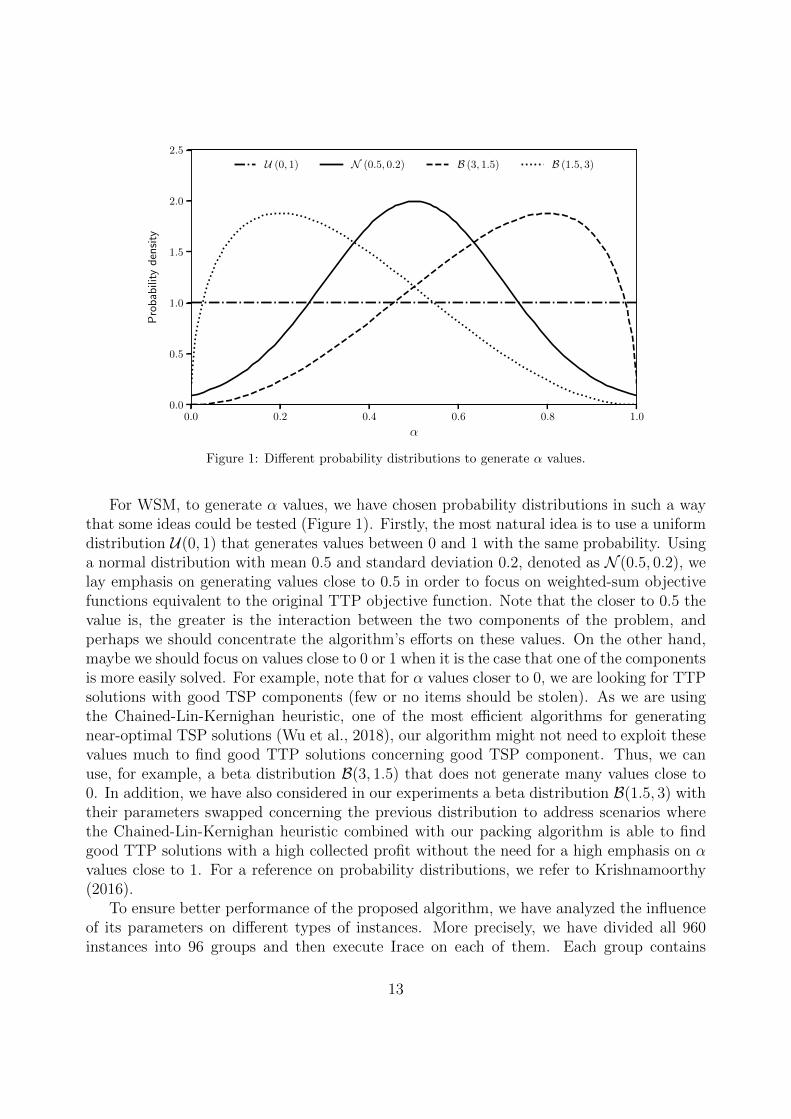
Figure 1: Different probability distributions to generate α values.

For WSM, to generate α values, we have chosen probability distributions in such a waythat some ideas could be tested (Figure 1). Firstly, the most natural idea is to use a uniformdistribution U(0, 1) that generates values between 0 and 1 with the same probability. Usinga normal distribution with mean 0.5 and standard deviation 0.2, denoted as N (0.5, 0.2), welay emphasis on generating values close to 0.5 in order to focus on weighted-sum objectivefunctions equivalent to the original TTP objective function. Note that the closer to 0.5 thevalue is, the greater is the interaction between the two components of the problem, andperhaps we should concentrate the algorithm’s efforts on these values. On the other hand,maybe we should focus on values close to 0 or 1 when it is the case that one of the componentsis more easily solved. For example, note that for α values closer to 0, we are looking for TTPsolutions with good TSP components (few or no items should be stolen). As we are usingthe Chained-Lin-Kernighan heuristic, one of the most efficient algorithms for generatingnear-optimal TSP solutions (Wu et al., 2018), our algorithm might not need to exploit thesevalues much to find good TTP solutions concerning good TSP component. Thus, we canuse, for example, a beta distribution B(3, 1.5) that does not generate many values close to0. In addition, we have also considered in our experiments a beta distribution B(1.5, 3) withtheir parameters swapped concerning the previous distribution to address scenarios wherethe Chained-Lin-Kernighan heuristic combined with our packing algorithm is able to findgood TTP solutions with a high collected profit without the need for a high emphasis on αvalues close to 1. For a reference on probability distributions, we refer to Krishnamoorthy(2016).

To ensure better performance of the proposed algorithm, we have analyzed the influenceof its parameters on different types of instances. More precisely, we have divided all 960instances into 96 groups and then execute Irace on each of them. Each group contains

13

all 10 instances defined with different sizes of knapsacks. These groups are identified asXXX YY ZZZ, in the same way as we have identified the instances, except for the lack of WW.With this approach, we would like to know whether there exist similar behaviors among thebest parameter configurations from different groups of instances. As we have selected 96groups with a large difference in characteristics among them, it is reasonable to think thatwhether such behaviors exist, they may also apply to unknown instances.

As Irace evaluates the quality of the output of a parameter configuration using a singlenumerical value, we should use for multi-objective problems some unary quality measure(Lopez-Ibanez et al., 2016b), such as the hypervolume indicator or the ε-measure (Zitzleret al., 2003). In our experiments, we have used the hypervolume indicator. In addition, wehave used all Irace default settings, except for the parameter maxExperiments, which hasbeen set to 1000. This parameter defines the stopping criteria of the tuning process. Werefer the readers to (Lopez-Ibanez et al., 2016a) for a complete user guide of Irace package.

From the tuning experiments, we have obtained the results shown in Figure 2. Eachparallel coordinate plot lists for each of the 96 groups (listed in the left-most column) theconfigurations returned by Irace (plotted in the other columns). As Irace can return morethan one configuration that are statistically indistinguishable given the threshold of thestatistical test, multiple configurations are sometimes shown. Each vertical axis indicatesa parameter and its range of values, and each configuration of parameters is described bya line that cuts each parallel axis in its corresponding value. Through the concentrationof the lines, we can see which parameter values have been most selected among all tuningexperiments. We have used different colors and styles for lines in order to emphasize theresults obtained for each group individually. All logs generated by the Irace executions, aswell as their settings can be found at the GitHub link along with our code.

We can make several observations from the tuning results. First, we notice that foralmost all groups of instances the uniform distribution U(0, 1) has been chosen. For somegroups, especially those that contain larger instances, other distributions have been returnedby Irace. Regarding the parameter η, we can observe a strong trend in increasing its valueas the number of cities increases. This is not too surprising, as the Chained-Lin-Kernighanheuristic, in general, requires more computational time to address larger TSP instances.Thus, computing a higher number of packing plans from each tour may generate betterBITTP solutions than resolve the TSP component many times. We can also observe fromthe values obtained for the parameter ρ that only a few attempts of our packing strategy areneeded to reach good results, which is especially true for larger instances. The low valuesobtained for the parameter γ for most groups of instances indicate that the frequency ofre-computation of the objective function in the packing algorithm may begin with low valueswithout interfering in the quality of the packing plan computed. Although the values of theparameter β do not follow a clear trend, they are strongly related to the number of citiesand mainly to the layout that the cities are arranged. For example, when many cities areuniformly arranged, the trend is towards low β values as, for this scenario, higher β valueswould probably not be efficient, since the algorithm would spend most of the time processingtoo many tours obtained from 2-opt moves. Finally, we can see that, in general, higher λvalues are concentrated in smaller-size instances, which is not surprising since the bit-flip

14

D η ρ γ β λ

eil51_10_unceil51_10_usweil51_10_bsceil51_05_unceil51_05_usweil51_05_bsceil51_03_unceil51_03_usweil51_03_bsceil51_01_unceil51_01_usweil51_01_bsc

U(0, 1)

N(0.5, 0.

2)

B(3, 1.

5)

B(1.5,

3)

0

50

100

150

200

0

25

50

75

100

0

50

100

150

200

-∞00.0

000010.0

00010.0

0010.0

010.0

10.1110100

0

0.1

0.2

0.3

0.4

0.5

D η ρ γ β λ

pr152_10_uncpr152_10_uswpr152_10_bscpr152_05_uncpr152_05_uswpr152_05_bscpr152_03_uncpr152_03_uswpr152_03_bscpr152_01_uncpr152_01_uswpr152_01_bsc

U(0, 1)

N(0.5, 0.

2)

B(3, 1.

5)

B(1.5,

3)

0

50

100

150

200

0

25

50

75

100

0

50

100

150

200

-∞00.0

000010.0

00010.0

0010.0

010.0

10.1110100

0

0.1

0.2

0.3

0.4

0.5

D η ρ γ β λ

a280_10_unca280_10_uswa280_10_bsca280_05_unca280_05_uswa280_05_bsca280_03_unca280_03_uswa280_03_bsca280_01_unca280_01_uswa280_01_bsc

U(0, 1)

N(0.5, 0.

2)

B(3, 1.

5)

B(1.5,

3)

0

50

100

150

200

0

25

50

75

100

0

50

100

150

200

-∞00.0

000010.0

00010.0

0010.0

010.0

10.1110100

0

0.1

0.2

0.3

0.4

0.5

D η ρ γ β λ

dsj1000_10_uncdsj1000_10_uswdsj1000_10_bscdsj1000_05_uncdsj1000_05_uswdsj1000_05_bscdsj1000_03_uncdsj1000_03_uswdsj1000_03_bscdsj1000_01_uncdsj1000_01_uswdsj1000_01_bsc

U(0, 1)

N(0.5, 0.

2)

B(3, 1.

5)

B(1.5,

3)

0

50

100

150

200

0

25

50

75

100

0

50

100

150

200

-∞00.0

000010.0

00010.0

0010.0

010.0

10.1110100

0

0.1

0.2

0.3

0.4

0.5

D η ρ γ β λ

fnl4461_10_uncfnl4461_10_uswfnl4461_10_bscfnl4461_05_uncfnl4461_05_uswfnl4461_05_bscfnl4461_03_uncfnl4461_03_uswfnl4461_03_bscfnl4461_01_uncfnl4461_01_uswfnl4461_01_bsc

U(0, 1)

N(0.5, 0.

2)

B(3, 1.

5)

B(1.5,

3)

0

50

100

150

200

0

25

50

75

100

0

50

100

150

200

-∞00.0

000010.0

00010.0

0010.0

010.0

10.1110100

0

0.1

0.2

0.3

0.4

0.5

D η ρ γ β λ

usa13509_10_uncusa13509_10_uswusa13509_10_bscusa13509_05_uncusa13509_05_uswusa13509_05_bscusa13509_03_uncusa13509_03_uswusa13509_03_bscusa13509_01_uncusa13509_01_uswusa13509_01_bsc

U(0, 1)

N(0.5, 0.

2)

B(3, 1.

5)

B(1.5,

3)

0

50

100

150

200

0

25

50

75

100

0

50

100

150

200

-∞00.0

000010.0

00010.0

0010.0

010.0

10.1110100

0

0.1

0.2

0.3

0.4

0.5

D η ρ γ β λ

pla33810_10_uncpla33810_10_uswpla33810_10_bscpla33810_05_uncpla33810_05_uswpla33810_05_bscpla33810_03_uncpla33810_03_uswpla33810_03_bscpla33810_01_uncpla33810_01_uswpla33810_01_bsc

U(0, 1)

N(0.5, 0.

2)

B(3, 1.

5)

B(1.5,

3)

0

50

100

150

200

0

25

50

75

100

0

50

100

150

200

-∞00.0

000010.0

00010.0

0010.0

010.0

10.1110100

0

0.1

0.2

0.3

0.4

0.5

D η ρ γ β λ

pla85900_10_uncpla85900_10_uswpla85900_10_bscpla85900_05_uncpla85900_05_uswpla85900_05_bscpla85900_03_uncpla85900_03_uswpla85900_03_bscpla85900_01_uncpla85900_01_uswpla85900_01_bsc

U(0, 1)

N(0.5, 0.

2)

B(3, 1.

5)

B(1.5,

3)

0

50

100

150

200

0

25

50

75

100

0

50

100

150

200

-∞00.0

000010.0

00010.0

0010.0

010.0

10.1110100

0

0.1

0.2

0.3

0.4

0.5

Figure 2: Irace results for the 96 groups of instances. Blue, green, red, and yellow lines represent, respectively,groups of instances with 1, 3, 5, and 10 items-per-city. Dashed, solid, and dotted lines are used, respectively,to emphasize the groups of instances with items where their weights and values are bounded and stronglycorrelated (bsc), uncorrelated with similar weights (usw), and uncorrelated (unc).

15

operator would perform too many moves on instances with many items and higher λ values.With a closer look, we can make additional observations by combining different param-

eters and characteristics of the instances. For example, η values are low for medium andlarge knapsack capacities (red and yellow) of eil51, while the opposite is true for the dsj1000instances, and other large instances. Across almost all instances, the η values are the lowestor among the lowest for instances with uncorrelated (dotted) knapsacks. For ρ, it is difficultto extract patterns, however, we can observe that the tuned configurations for instanceswith strongly correlated knapsacks (dashed) have the highest ρ values for the groups eil51(red), pr152 (blue), and fnl4661 (blue). For γ, small knapsacks (blue) with uncorrelated butsimilar weights (solid) result in high or the highest values for eil51, pr152, and pla33810,but for example not for a280. For β, we cannot observe clear trends for the knapsack type,however, sometimes the knapsack capacity stands out. For example, for a280, the smallestknapsacks (blue) resulted in the highest values, while blue has the lowest values for dsj1000,and the largest knapsacks resulted in the highest values (yellow) for the tuning experimentsfor the pla33810 group. We can observe similar ‘inversions’ also for γ. There, for exam-ple the smallest knapsacks with uncorrelated and similar weights (blue, solid) result in thesmallest values on some instance groups, but for the largest values on others.

In summary, we can observe many consistent as well as inconsistent patterns for thedifferent groups of instances, and depending on the knapsack type and the knapsack capacity.In combination with instance features (e.g. the ones from Wagner et al. (2018)), this mightmake for an interesting challenge for per-instance-algorithm-configuration (Hutter et al.,2006), however, this is beyond the scope of the present study.

In a final experiment, we investigate the extent to which the results so far can carryover to unseen instances. To achieve this, we use the average of the parameter values(and the mode for the categorical parameters) obtained from the tuning experiments tofurnish a single configuration of parameters for unknown instances, and then investigatethat configuration’s performance. The configuration is: D = U(0, 1), η = 117, ρ = 12,γ = 41, β = 0.001, and λ = 0.22. In order to confirm whether these values are a reasonableconfiguration of parameters for our algorithm, we have randomly chosen 10 unknown (fromthe perspective of the tuning experiments) groups of instances from the instances definedby Polyakovskiy et al. (2014), and compared the results obtained with the aforementionedconfiguration against the best configuration for each group. To find out which is the bestconfiguration of parameters for each of these 10 groups, we have again used Irace in thesame way as described before. As each group has 10 instances, we have 100 instances intotal. For each of them and for each of the two different configurations of parameters, wehave run our algorithm 30 times and used average values of hypervolumes achieved to plotFigure 3. There, two sets stand out: (i) on the pr76 instances the tuned configurationperforms better; and (ii) on the rl11849 the general parameter configuration is sometimesworse and sometimes better. On all other instances, the different configurations (general vs.best configuration) perform essentially the same.

16

Hypervolum

e

General parameter configurationBest parameter configurations

st70_03_usw_01

st70_03_usw_02

st70_03_usw_03

st70_03_usw_04

st70_03_usw_05

st70_03_usw_06

st70_03_usw_07

st70_03_usw_08

st70_03_usw_09

st70_03_usw_10

pr76_10_usw_01

pr76_10_usw_02

pr76_10_usw_03

pr76_10_usw_04

pr76_10_usw_05

pr76_10_usw_06

pr76_10_usw_07

pr76_10_usw_08

pr76_10_usw_09

pr76_10_usw_10

rat99_03_bsc_01

rat99_03_bsc_02

rat99_03_bsc_03

rat99_03_bsc_04

rat99_03_bsc_05

rat99_03_bsc_06

rat99_03_bsc_07

rat99_03_bsc_08

rat99_03_bsc_09

rat99_03_bsc_10

gil262_03_usw_01

gil262_03_usw_02

gil262_03_usw_03

gil262_03_usw_04

gil262_03_usw_05

gil262_03_usw_06

gil262_03_usw_07

gil262_03_usw_08

gil262_03_usw_09

gil262_03_usw_10

pr299_05_bsc_01

pr299_05_bsc_02

pr299_05_bsc_03

pr299_05_bsc_04

pr299_05_bsc_05

pr299_05_bsc_06

pr299_05_bsc_07

pr299_05_bsc_08

pr299_05_bsc_09

pr299_05_bsc_10

0.75

0.8

0.85

0.9

0.95

Hypervolum

epcb44205_unc_01

pcb44205_unc_02

pcb44205_unc_03

pcb44205_unc_04

pcb44205_unc_05

pcb44205_unc_06

pcb44205_unc_07

pcb44205_unc_08

pcb44205_unc_09

pcb44205_unc_10

d657_01_bsc_01

d657_01_bsc_02

d657_01_bsc_03

d657_01_bsc_04

d657_01_bsc_05

d657_01_bsc_06

d657_01_bsc_07

d657_01_bsc_08

d657_01_bsc_09

d657_01_bsc_10

pr1002_03_unc_01

pr1002_03_unc_02

pr1002_03_unc_03

pr1002_03_unc_04

pr1002_03_unc_05

pr1002_03_unc_06

pr1002_03_unc_07

pr1002_03_unc_08

pr1002_03_unc_09

pr1002_03_unc_10

rl11849_10_bsc_01

rl11849_10_bsc_02

rl11849_10_bsc_03

rl11849_10_bsc_04

rl11849_10_bsc_05

rl11849_10_bsc_06

rl11849_10_bsc_07

rl11849_10_bsc_08

rl11849_10_bsc_09

rl11849_10_bsc_10

pcb1173_01_bsc_01

pcb1173_01_bsc_02

pcb1173_01_bsc_03

pcb1173_01_bsc_04

pcb1173_01_bsc_05

pcb1173_01_bsc_06

pcb1173_01_bsc_07

pcb1173_01_bsc_08

pcb1173_01_bsc_09

pcb1173_01_bsc_10

0.75

0.8

0.85

0.9

0.95

Figure 3: Average hypervolume on 100 unseen instances. Shown are the results for the best (irace-tuned)parameter configuration (per instance) and of the general (“averaged”) parameter configuration from earlierexperiments.

17

4.3. WSM vs. NDSBRKGA

In the first analysis that assesses the quality of our WSM, we compare the solutionsobtained by it with the solutions obtained by NDSBRKGA proposed by Chagas et al. (2020).In order to make a fair comparison, we have tuned the parameters of the NDSBRKGAfollowing the same procedure used in the tuning of the parameters of WSM. The parametervalues considered for these experiments have been chosen based on the insights reportedin (Chagas et al., 2020). These parameter values, as well as the results obtained in theexperiment, are available at the GitHub link along with our other files.5

Due to the randomized nature of both algorithms, we have performed 30 independentrepetitions on each instance. Each run has been executed for 10 minutes with the bestparameter values found in the tuning experiments.

As in (Chagas et al., 2020), we have used the hypervolume indicator (HV) (Zitzler andThiele, 1998) as a performance indicator to compare and analyze the results obtained. Thisindicator is one of the most used indicators for measuring the quality of a set of non-dominated solutions by calculating the volume of the dominated portion of the objectivespace bounded from a reference point. To make the hypervolume suitable for the comparisonof objectives with greatly varying ranges, a normalization of objective values is commonlydone beforehand. Therefore, before computing the hypervolume, we have first normalizedthe objective values between 0 and 1 according to their minimum and maximum value foundduring our experiments. Although maximizing the hypervolume might not be equivalent tofinding the optimal approximation to the Pareto-optimal front (Bringmann and Friedrich,2013; Wagner et al., 2015), we have assumed that the higher the hypervolume indicator, thebetter the solution sets are, as is commonly considered in the literature.

We compare the performance of the solutions obtained by measuring for each instancethe percentage variation of the average hypervolume obtained considering the independentruns of each algorithm. More precisely, for each instance, we have estimated the referencepoint as the maximum travel time and the minimum profit obtained from the non-dominatedsolutions, which have been extracted from all solutions returned by the algorithms. Then, wehave computed the hypervolume covered by the non-dominated solutions found by each runof each algorithm according to the estimated reference point. Thereafter, we can computethe percentage variation as(

HVWSMavg − HVNDSBRKGA

avg

)/ max

(HVWSM

avg ,HVNDSBRKGAavg

)· 100%

, where HVWSMavg and HVNDSBRKGA

avg are, respectively, the average hypervolumes obtained byWSM and NDSBRKGA in their independent executions.

In Figure 4, we visualise the percentage variations of the average hypervolumes usinga heatmap to emphasize larger variations. Each cell of the heatmap informs the results

5As neither the HPI algorithm nor the HPI implementation are available, we could not include HPI inthis tuning-based comparison. HPI has been the result of a classroom setting and their actual results havebeen (to some extent) aggregated across multiple teams (and hence implementations), which has been legalw.r.t. the competition rules (as said competition required only the solution files, not any implementations).

18

-15

-10

-5

0

5

10

15

20

25

bsc_01

bsc_02

bsc_03

bsc_04

bsc_05

bsc_06

bsc_07

bsc_08

bsc_09

bsc_10

unc_01

unc_02

unc_03

unc_04

unc_05

unc_06

unc_07

unc_08

unc_09

unc_10

usw_01

usw_02

usw_03

usw_04

usw_05

usw_06

usw_07

usw_08

usw_09

usw_10

eil51_01eil51_03eil51_05eil51_10pr152_01pr152_03pr152_05pr152_10a280_01a280_03a280_05a280_10dsj1000_01dsj1000_03dsj1000_05dsj1000_10fnl4461_01fnl4461_03fnl4461_05fnl4461_10usa13509_01usa13509_03usa13509_05usa13509_10pla33810_01pla33810_03pla33810_05pla33810_10pla85900_01pla85900_03pla85900_05pla85900_10

Figure 4: Percentage variation of the average hypervolumes. Shades of orange and red indicate in whichinstances our WSM has reached a higher hypervolume than NDSBRKGA, while shades of blue indicate theopposite.

obtained for a specific instance. Note that the vertical axis depicts the characteristics XXX

and YY of instances, while the horizontal axis depicts the characteristics ZZZ and WW. Notealso that positive variation values (highlighted in shades of orange and red) indicate thatour WSM has reached a higher hypervolume, while negative variation values (highlighted inshades of blue) indicate the opposite behavior. Besides, the higher the absolute value (moreintense color), the higher the difference between the hypervolumes.

From Figure 4, we can observe that our WSM is clearly more effective than NDSBRKGAfor larger instances. This is especially true for instances with the smallest knapsack capaci-ties. Note that, in general, the smaller the size is of the knapsack, the higher the performanceis of WSM concerning the NDSBRKGA.

Note that, although our solutions still cover a higher hypervolume for larger instanceswith uncorrelated (unc) items, it must be stressed that our WSM has obtained the worseperformance regarding the NDSBRKGA for these instances. This behavior could be ex-plained by the fact that our packing heuristic might present difficulties in dealing with thoseitems because when there is no correlation between their profits and weights and the weightspresent a large variety, our packing algorithm may not be able to create a good order of the

19

items for our packing strategy. This is interesting, as unc knapsacks are not necessarily seenas difficult (Martello et al., 1999); but in our algorithm, they might end up being due to ourstrategy for solving the KP component. Another fact that could explain the worse perfor-mance of WSM on instances with uncorrelated items would be that NDSBRKGA has a goodperformance for these instances, making the performance of our algorithm less prominent.

Regarding the smaller-size instances, both algorithms have achieved similar performance(almost blank cells). However, with a closer look at Figure 4, we can see a slightly betterperformance of NDSBRKGA. To better analyze these results, we have used another per-formance measure. For each instance we have merged all the solutions found in order toextract from them a single non-dominated set of solutions. Then, we have computed howmany non-dominated solutions have been obtained by each algorithm. Our purpose of thisanalysis is to evaluate both algorithms regarding their ability to find non-dominated solu-tions with different objective values. Therefore, duplicate solutions regarding their objectivevalues have been removed, i.e., we have regarded a single non-dominated solution with thesame values in both objectives. In Figure 5, we present these numbers in percentages ac-cording to the total number of non-dominated solutions following the heatmap scheme usedpreviously.

The results shown in Figure 5 corroborate those shown in Figure 4. As was expected, ouralgorithm has found more non-dominated solutions especially for those instances where itobtained a higher hypervolume. However, even for the instances in which the NDSBRKGAfound better solutions, the difference between the hypervolumes of both algorithms remainslow.

To statistically compare the performance of the algorithms, we have used the Wilcoxonsigned-rank test on the hypervolumes achieved in the 30 independent runs. With a signifi-cance level of 5%, there is no statistical difference between both algorithms in 27 instances(2.8%), our algorithm is significantly better in 789 instances (82.2%) and worse in 144 (15%)ones when compared to NDSBRKGA.

4.4. WSM vs. competition results

Next, we compare WSM to the results of the BITTP competitions held at EMO20196

and GECCO20197. Both competitions have used the same rules and criteria. There were noregulations regarding the running time and the number of processors used. The final rankingused for the competitions was solely based on the solution set submitted by each participantfor nine medium/large TTP instances chosen from the TTP benchmark (Polyakovskiy et al.,2014). More precisely, the final ranking was defined according to the hypervolume coveredby the solutions. To calculate the hypervolumes, the reference points have been defined asthe maximum time and the minimum profit obtained from the non-dominated solutions,which have been built from all submitted solutions. In order to make a fair ranking, themaximum number of solutions allowed for each instance has been limited. In Table 2, welist the instances used as well as the maximum number of solutions allowed.

6https://www.egr.msu.edu/coinlab/blankjul/emo19-thief/7https://www.egr.msu.edu/coinlab/blankjul/gecco19-thief/

20

0

10

20

30

40

50

60

70

80

90

100

bsc_01

bsc_02

bsc_03

bsc_04

bsc_05

bsc_06

bsc_07

bsc_08

bsc_09

bsc_10

unc_01

unc_02

unc_03

unc_04

unc_05

unc_06

unc_07

unc_08

unc_09

unc_10

usw_01

usw_02

usw_03

usw_04

usw_05

usw_06

usw_07

usw_08

usw_09

usw_10

eil51_01eil51_03eil51_05eil51_10pr152_01pr152_03pr152_05pr152_10a280_01a280_03a280_05a280_10dsj1000_01dsj1000_03dsj1000_05dsj1000_10fnl4461_01fnl4461_03fnl4461_05fnl4461_10usa13509_01usa13509_03usa13509_05usa13509_10pla33810_01pla33810_03pla33810_05pla33810_10pla85900_01pla85900_03pla85900_05pla85900_10

(a) NDSBRKGA

0

10

20

30

40

50

60

70

80

90

100

bsc_01

bsc_02

bsc_03

bsc_04

bsc_05

bsc_06

bsc_07

bsc_08

bsc_09

bsc_10

unc_01

unc_02

unc_03

unc_04

unc_05

unc_06

unc_07

unc_08

unc_09

unc_10

usw_01

usw_02

usw_03

usw_04

usw_05

usw_06

usw_07

usw_08

usw_09

usw_10

eil51_01eil51_03eil51_05eil51_10pr152_01pr152_03pr152_05pr152_10a280_01a280_03a280_05a280_10dsj1000_01dsj1000_03dsj1000_05dsj1000_10fnl4461_01fnl4461_03fnl4461_05fnl4461_10usa13509_01usa13509_03usa13509_05usa13509_10pla33810_01pla33810_03pla33810_05pla33810_10pla85900_01pla85900_03pla85900_05pla85900_10

(b) WSM

Figure 5: Percentage of non-dominated solutions found by each algorithm.

21

Table 2: Maximum number of solutions allowed by each TTP instance used in the BITTP competitions.

InstanceMaximum number of

solutions allowed

a280 01 bsc 01 100a280 05 usw 05 100a280 10 unc 10 100

fnl4461 01 bsc 01 50fnl4461 05 usw 05 50fnl4461 10 unc 10 50

pla33810 01 bsc 01 20pla33810 05 usw 05 20pla33810 10 unc 10 20

As our algorithm can return a higher number of solutions than those reported in Table 2,we have used the dynamic programming algorithm developed by Auger et al. (2009) in orderto find a subset of limited size of the returned solutions such that their hypervolume indicatoris maximal. As stated by Auger et al. (2009), this dynamic programming can be solved intime O(|A|3), where A would be the set of solutions returned by our algorithm. Note thatthe application of this strategy has also been used in (Chagas et al., 2020) for NDSBRKGA,and it is only part of a post-processing needed to fit both algorithms to the competitioncriteria.

In both competitions, preliminary versions of NDSBRKGA have been submitted as jo-mar, a reference to the two authors (Jonatas and Marcone) who first worked on thatalgorithm. These preliminary versions are presented in (Chagas et al., 2020) as well as theirresults achieved in both competitions. In short, jomar has won the first and second places,at EMO2019 and GECCO2019 competitions, respectively. After the competitions, someimprovements have been incorporated in the preliminary versions of NDSBRKGA, resultingin its final version as is described in (Chagas et al., 2020). In the following, we compareour WSM with that final version as it presents slightly better results concerning its previousones.

In Table 3, we present for each instance the best results submitted for the competitionsand also the results obtained by our WSM. The results of all submissions can be found atweb pages previously reported. As the final results of NDSBRKGA have been obtainedwith 5 hours of processing, we have executed our algorithm for 5 hours as well to make afair comparison. We would like to mention that we have no information on how the otherparticipants have obtained their results. As we stated before, there were no regulationsregarding the running time and the number of processors used. In both competitions,their rankings have been solely based on the solution set submitted by each participant.Furthermore, to the best of our knowledge, there is no description available of the solutionapproaches submitted.

From Table 3, we can notice that WSM has obtained better performance on large-size

22

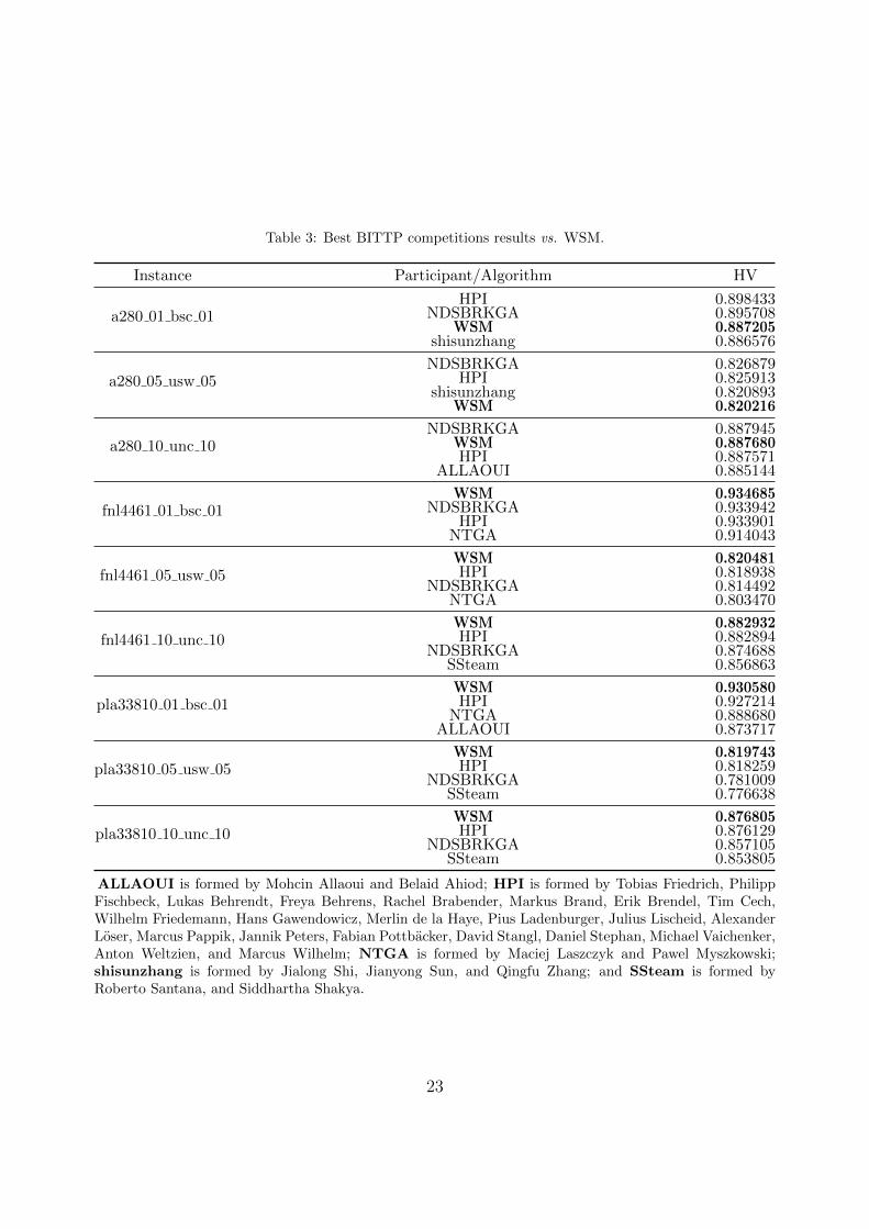
Table 3: Best BITTP competitions results vs. WSM.

Instance Participant/Algorithm HV

a280 01 bsc 01HPI 0.898433

NDSBRKGA 0.895708WSM 0.887205

shisunzhang 0.886576

a280 05 usw 05NDSBRKGA 0.826879

HPI 0.825913shisunzhang 0.820893

WSM 0.820216

a280 10 unc 10NDSBRKGA 0.887945

WSM 0.887680HPI 0.887571

ALLAOUI 0.885144

fnl4461 01 bsc 01WSM 0.934685

NDSBRKGA 0.933942HPI 0.933901

NTGA 0.914043

fnl4461 05 usw 05WSM 0.820481HPI 0.818938

NDSBRKGA 0.814492NTGA 0.803470

fnl4461 10 unc 10WSM 0.882932HPI 0.882894

NDSBRKGA 0.874688SSteam 0.856863

pla33810 01 bsc 01WSM 0.930580HPI 0.927214

NTGA 0.888680ALLAOUI 0.873717

pla33810 05 usw 05WSM 0.819743HPI 0.818259

NDSBRKGA 0.781009SSteam 0.776638

pla33810 10 unc 10WSM 0.876805HPI 0.876129

NDSBRKGA 0.857105SSteam 0.853805

ALLAOUI is formed by Mohcin Allaoui and Belaid Ahiod; HPI is formed by Tobias Friedrich, PhilippFischbeck, Lukas Behrendt, Freya Behrens, Rachel Brabender, Markus Brand, Erik Brendel, Tim Cech,Wilhelm Friedemann, Hans Gawendowicz, Merlin de la Haye, Pius Ladenburger, Julius Lischeid, AlexanderLoser, Marcus Pappik, Jannik Peters, Fabian Pottbacker, David Stangl, Daniel Stephan, Michael Vaichenker,Anton Weltzien, and Marcus Wilhelm; NTGA is formed by Maciej Laszczyk and Pawel Myszkowski;shisunzhang is formed by Jialong Shi, Jianyong Sun, and Qingfu Zhang; and SSteam is formed byRoberto Santana, and Siddhartha Shakya.

23

instances. For the three smallest instances, it has presented the worst results concerningthe other results, especially, for those reached by the first (HPI) and second (NDSBRKGA)places at GECCO2019 competition. For the other instances, our results have surpassed allother submissions with a larger difference compared to NDSBRKGA. In Figure 6, we showthe hypervolume achieved by WSM over runtime. In order to make a visual comparison, wehave plotted on horizontal lines the (final) hypervolume achieved by the two best algorithms(HPI and NDSBRKGA) of the competitions. One can see that our WSM is able to findsolutions that cover a high hypervolume even with low computational time.

4.5. Dispersed distribution of the non-dominated solutions

We now analyze the dispersion over the objective spaces of the solutions found by ouralgorithm. As we have stated before, a limitation of WSMs is the fact that, even with aconsistent change in weights attributed to the objectives, they may not generate a disperseddistribution of non-dominated solutions found. This limitation does not affect our WSM, asit can be seen in Figure 7, where we have plotted the objective values of all non-dominatedsolutions found by WSM with 10 minutes of runtime for the nine medium/large-size instancesused in the aforementioned BITTP competitions. In addition, we have highlighted whichα has been used when finding each solution. One can notice dispersed distributions of thesolutions as well as the α values. Moreover, as expected, lower α values produce solutionswith faster tours, with higher ones produce solutions with good packing plans.

4.6. Single-objective comparison

Since BITTP is a bi-objective formulation created from the TTP without introducingany new specification or removing any original constraint, any feasible BITTP solution isalso feasible for the TTP. Thus, we can measure the performance of the solutions obtainedby our algorithm according to their single-objective TTP scores. However, it is importantto emphasize that our algorithm has not been developed with a single-objective purpose.Therefore, we should be careful when comparing it with other algorithms for the TTP.

A fairer comparison can be achieved between our results and those reached by NDS-BRKGA, as both approaches have been developed with the same ambition. For this purpose,we have calculated for each instance the Relative Percentage Difference (RPD) between thebest TTP scores achieved by WSM and NDSBRKGA, referenced as SWSM

best and SNDSBRKGAbest ,

respectively. It is important to emphasize that no additional tests have been performed, weonly choose the solution with the best TTP score among the non-dominated solutions foundby each algorithm on each instance. The RPD metric has been calculated as(

SWSMbest − SNDSBRKGA

best

) / ∣∣SNDSBRKGAbest

∣∣ · 100%

, and we plot its values using a heatmap in order to highlight higher differences as depictedin Figure 8. Note that positive values (highlighted in shades of orange and red) indicatethat our WSM has found higher TTP scores.

We can note that the heatmap show in Figure 8 has characteristics similar to those inFigure 5b, where higher percentages of the number of non-dominated solutions found by our

24

a280 01 bsc 01

Runtime

Hypervolum

e

10min

20min

30min 1h 2h 3h 5h

0.885

0.89

0.895

0.9

a280 05 usw 05

Runtime

Hypervolum

e

10min

20min

30min 1h 2h 3h 5h

0.815

0.82

0.825

0.83

a280 10 unc 10

Runtime

Hypervolum

e

10min

20min

30min 1h 2h 3h 5h

0.8875

0.88775

0.888

fnl4461 01 bsc 01

Runtime

Hypervolum

e

10min

20min

30min 1h 2h 3h 5h

0.933

0.934

0.935

fnl4461 05 usw 05

Runtime

Hypervolum

e

10min

20min

30min 1h 2h 3h 5h

0.8125

0.815

0.8175

0.82

0.8225

fnl4461 10 unc 10

Runtime

Hypervolum

e

10min

20min

30min 1h 2h 3h 5h

0.87

0.875

0.88

0.885

pla33810 01 bsc 01

Runtime

Hypervolum

e

10min

20min

30min 1h 2h 3h 5h

0.85

0.9

0.95

pla33810 05 usw 05

Runtime

Hypervolum

e

10min

20min

30min 1h 2h 3h 5h

0.775

0.8

0.825

pla33810 10 unc 10

Runtime

Hypervolum

e

10min

20min

30min 1h 2h 3h 5h

0.85

0.86

0.87

0.88

HPINDSBRKGA

Runtime

Hypervo

lume

0.85

0.86

0.87

0.88 HPINDSBRKGA

Runtime

Hypervo

lume

0.85

0.86

0.87

0.88

Figure 6: Hypervolume of WSM over time versus the hypervolume of HPI and NDSBRKGA; for the lattertwo, only the final hypervolume is known.

25

a280 01 bsc 01

h(π, z)

g(z)

5k 7.5k0

22k

44k

a280 05 usw 05

h(π, z)

g(z)

4k 6k0

250k

500k

a280 10 unc 10

h(π, z)

g(z)

4k 6k0

700k

1 400k

fnl4461 01 bsc 01

h(π, z)

g(z)

200k 300k 400k0

330k

660k

fnl4461 05 usw 05

h(π, z)

g(z)

200k 300k 400k0

3 750k

7.5M

fnl4461 10 unc 10

h(π, z)

g(z)

200k 300k 400k0

11M

22M

pla33810 01 bsc 01

h(π, z)

g(z)

100M 150M0

2.5M

5M

pla33810 05 usw 05

h(π, z)

g(z)

100M 150M0

30M

60M

pla33810 10 unc 10

h(π, z)

g(z)

100M 150M0

85M

170M

þÿ�h�(�À�,� �z�)

g(z)

0 0.1 0.2 0.3 0.4 0.5 0.6 0.7 0.8 0.9 1

500 550 600 650 700 7500

8k

Figure 7: Non-dominated points found by WSM. Colors indicate the α values used when finding each point.

26

-50

-25

0

25

50

75

100

125

150

175

200

bsc_01

bsc_02

bsc_03

bsc_04

bsc_05

bsc_06

bsc_07

bsc_08

bsc_09

bsc_10

unc_01

unc_02

unc_03

unc_04

unc_05

unc_06

unc_07

unc_08

unc_09

unc_10

usw_01

usw_02

usw_03

usw_04

usw_05

usw_06

usw_07

usw_08

usw_09

usw_10

eil51_01eil51_03eil51_05eil51_10pr152_01pr152_03pr152_05pr152_10a280_01a280_03a280_05a280_10dsj1000_01dsj1000_03dsj1000_05dsj1000_10fnl4461_01fnl4461_03fnl4461_05fnl4461_10usa13509_01usa13509_03usa13509_05usa13509_10pla33810_01pla33810_03pla33810_05pla33810_10pla85900_01pla85900_03pla85900_05pla85900_10

Figure 8: WSM vs. NDSBRKGA according to their obtained single-objective TTP scores. Shades oforange and red indicate in which instances our WSM has reached better single-objective TTP scores thanNDSBRKGA, while shades of blue indicate the opposite.

27

algorithm are highlighted. Therefore, this behavior is not surprising, since dominated solu-tions have essentially lower TTP scores compared to the non-dominated solutions. Thus, wecan confirm a better efficiency of WSM also concerning the TTP scores for larger instances,while its worst performance on smaller-size instances is less expressive.

Although it may not be fair, as we stated earlier, we conclude our analysis by comparingthe best TTP scores obtained by WSM with the best single TTP objective scores reportedin (Wagner et al., 2018), where the authors have made a comprehensive comparison of 21algorithms proposed for the TTP over the years. In this comparison, we use again the RPDmetric, which now is calculated for each instance as(

SWSMbest − S21ALGS

best

) / ∣∣S21ALGSbest

∣∣ · 100%

, where S21ALGSbest indicates the best TTP score found among all 21 algorithms analyzed in

(Wagner et al., 2018). In Figure 9, we plot the calculated RPD values following the samevisualization scheme adopted previously. In addition, we highlight with a diamond symbolthe instances for which our algorithm has found better solutions.

One can note that, in general, our results presented worse performance, which is es-pecially true for the smaller-size instances. However, for 379 instances our results haveoutperformed all 21 TTP algorithms. This shows that our WSM can also be competitive tosolve the TTP.

5. Conclusions

In this work, we have addressed a bi-objective formulation of the Traveling Thief Prob-lem (TTP), an academic multi-component problem that combines two classic combinatorialoptimization problems: the Traveling Salesperson Problem and the Knapsack Problem.For solving the problem, we have proposed a heuristic algorithm based on the well-knownweighted-sum method, in which the objective functions are summed up with varying weightsand then the problem is optimized in relation to the single-objective function formed by thissum. Our algorithm combines exploration and exploitation search procedures by using effi-cient operators, as well as known strategies for the single-objective TTP; among these aredeterministic strategies that we have randomized here. We have studied the effects of ouralgorithmic components by performing extensive tuning of their parameters over differentgroups of instances. This tuning also shows that different configurations are needed depend-ing on the instance group, the knapsack type, and the knapsack capacity. Our comparisonwith multi-objective approaches shows that we outperform participants of recent optimiza-tion competitions, and we have furthermore found new best solutions for 379 instances tothe single-objective case along the way.

For future research, we would like to point out as a promising direction the investigationof the influence of different algorithmic components already proposed in the literature overdifferent instance characteristics by investigating tuned configurations. Studies in this data-driven direction have achieved important insights to design better single-objective solvers forfundamental problems and real-world problems (see, e.g. Section “Research Directions” of

28

-30

-25

-20

-15

-10

-5

0

5

10

15

bsc_01

bsc_02

bsc_03

bsc_04

bsc_05

bsc_06

bsc_07

bsc_08

bsc_09

bsc_10

unc_01

unc_02

unc_03

unc_04

unc_05

unc_06

unc_07

unc_08

unc_09

unc_10

usw_01

usw_02

usw_03

usw_04

usw_05

usw_06

usw_07

usw_08

usw_09

usw_10

eil51_01eil51_03eil51_05eil51_10pr152_01pr152_03pr152_05pr152_10a280_01a280_03a280_05a280_10dsj1000_01dsj1000_03dsj1000_05dsj1000_10fnl4461_01fnl4461_03fnl4461_05fnl4461_10usa13509_01usa13509_03usa13509_05usa13509_10pla33810_01pla33810_03pla33810_05pla33810_10pla85900_01pla85900_03pla85900_05pla85900_10

Figure 9: WSM vs. TTP algorithms according to their obtained single-objective TTP scores. Shades oforange and red indicate in which instances our WSM has reached better single-objective TTP scores than thebest algorithm among 21 ones reported in (Wagner et al., 2018), while shades of blue indicate the opposite.Diamond symbols highlight the 379 instances on which our WSM has found better results.

29

Agrawal et al. (2020)). Another interesting direction would be to use our algorithm core ideafor solving other multi-objective problems with multiple interacting components. By coreidea, we refer to how to explore and exploit the space of solutions once efficient operatorsand strategies are known for solving different components of a multi-objective problem.

Acknowledgments. This study has been financed in part by Coordenacao de Aperfeicoa-mento de Pessoal de Nıvel Superior - Brazil (CAPES) - Finance code 001. The authors wouldalso like to thank Fundacao de Amparo a Pesquisa do Estado de Minas Gerais (FAPEMIG),Conselho Nacional de Desenvolvimento Cientıfico e Tecnologico (CNPq), Universidade Fed-eral de Ouro Preto (UFOP) and Universidade Federal de Vicosa (UFV) for supporting thisresearch. Markus Wagner would like to acknowledge support by the Australian ResearchCouncil Project DP200102364.

References

Agrawal, A., Menzies, T., Minku, L.L., Wagner, M., Yu, Z., 2020. Better software analytics via” duo”: Datamining algorithms using/used-by optimizers. Empirical Software Engineering 25, 2099–2136.

Applegate, D., Cook, W., Rohe, A., 2003. Chained lin-kernighan for large traveling salesman problems.INFORMS Journal on Computing 15, 82–92.

Auger, A., Bader, J., Brockhoff, D., Zitzler, E., 2009. Investigating and exploiting the bias of the weightedhypervolume to articulate user preferences, in: Proceedings of the Genetic and Evolutionary ComputationConference, ACM. pp. 563–570.

Birattari, M., Yuan, Z., Balaprakash, P., Stutzle, T., 2010. F-race and iterated f-race: An overview, in:Experimental methods for the analysis of optimization algorithms. Springer, pp. 311–336.

Blank, J., Deb, K., Mostaghim, S., 2017. Solving the Bi-objective Traveling Thief Problem with Multi-objective Evolutionary Algorithms. Springer. pp. 46–60.

Bonyadi, M.R., Michalewicz, Z., Barone, L., 2013. The travelling thief problem: The first step in thetransition from theoretical problems to realistic problems, in: 2013 IEEE Congress on EvolutionaryComputation, IEEE. pp. 1037–1044.

Bonyadi, M.R., Michalewicz, Z., Przybylek, M.R., Wierzbicki, A., 2014. Socially inspired algorithms for theTTP, in: Proceedings of the Genetic and Evolutionary Computation Conference, ACM. pp. 421–428.

Bonyadi, M.R., Michalewicz, Z., Wagner, M., Neumann, F., 2019. Evolutionary Computation for Multi-component Problems: Opportunities and Future Directions. Springer. pp. 13–30.

Bringmann, K., Friedrich, T., 2013. Approximation quality of the hypervolume indicator. Artificial Intelli-gence 195, 265 – 290.

Chagas, J.B.C., Blank, J., Wagner, M., Souza, M.J.F., Deb, K., 2020. A non-dominated sorting based cus-tomized random-key genetic algorithm for the bi-objective traveling thief problem. Journal of Heuristics.

Chand, S., Wagner, M., 2016. Fast heuristics for the multiple traveling thieves problem, in: Proceedings ofthe Genetic and Evolutionary Computation Conference, ACM. pp. 293–300.

Cheng, B., Yang, Y., Hu, X., 2016. Supply chain scheduling with batching, production and distribution.International Journal of Computer Integrated Manufacturing 29, 251–262.

Crepinsek, M., Liu, S.H., Mernik, M., 2013. Exploration and exploitation in evolutionary algorithms: Asurvey. ACM computing surveys (CSUR) 45, 1–33.

Das, I., Dennis, J.E., 1997. A closer look at drawbacks of minimizing weighted sums of objectives for paretoset generation in multicriteria optimization problems. Structural optimization 14, 63–69.

El Yafrani, M., Ahiod, B., 2015. Cosolver2b: an efficient local search heuristic for the travelling thief problem,in: 2015 IEEE ACS 12th International Conference of Computer Systems and Applications (AICCSA),IEEE. pp. 1–5.

30

El Yafrani, M., Ahiod, B., 2016. Population-based vs. single-solution heuristics for the travelling thiefproblem, in: Proceedings of the Genetic and Evolutionary Computation Conference, ACM. pp. 317–324.

El Yafrani, M., Ahiod, B., 2018. Efficiently solving the traveling thief problem using hill climbing andsimulated annealing. Information Sciences 432, 231–244.

Faulkner, H., Polyakovskiy, S., Schultz, T., Wagner, M., 2015. Approximate approaches to the traveling thiefproblem, in: Proceedings of the Genetic and Evolutionary Computation Conference, ACM. pp. 385–392.

Forster, F., Bortfeldt, A., 2012. A tree search procedure for the container relocation problem. Computers& Operations Research 39, 299–309.

Galand, L., Spanjaard, O., 2012. Exact algorithms for owa-optimization in multiobjective spanning treeproblems. Computers & Operations Research 39, 1540–1554.

Hottung, A., Tanaka, S., Tierney, K., 2020. Deep learning assisted heuristic tree search for the containerpre-marshalling problem. Computers & Operations Research 113, 104781.

Hutter, F., Hamadi, Y., Hoos, H.H., Leyton-Brown, K., 2006. Performance prediction and automatedtuning of randomized and parametric algorithms, in: Principles and Practice of Constraint Programming,Springer. pp. 213–228.

Iori, M., Martello, S., 2010. Routing problems with loading constraints. Top 18, 4–27.Jin, B., Zhu, W., Lim, A., 2015. Solving the container relocation problem by an improved greedy look-ahead

heuristic. European Journal of Operational Research 240, 837–847.Klamroth, K., Mostaghim, S., Naujoks, B., Poles, S., Purshouse, R., Rudolph, G., Ruzika, S., Sayın, S.,

Wiecek, M.M., Yao, X., 2017. Multiobjective optimization for interwoven systems. Journal of Multi-Criteria Decision Analysis 24, 71–81.

Krishnamoorthy, K., 2016. Handbook of statistical distributions with applications. CRC Press.Lopez-Ibanez, M., Caceres, L.P., Dubois-Lacoste, J., Stutzle, T., Birattari, M., 2016a. The irace package:

User guide. IRIDIA, Universite Libre de Bruxelles, Belgium, Tech. Rep. TR/IRIDIA/2016-004 .Lopez-Ibanez, M., Dubois-Lacoste, J., Caceres, L.P., Birattari, M., Stutzle, T., 2016b. The irace package:

Iterated racing for automatic algorithm configuration. Operations Research Perspectives 3, 43–58.Maity, A., Das, S., 2020. Efficient hybrid local search heuristics for solving the travelling thief problem.

Applied Soft Computing , 106284.Marler, R.T., Arora, J.S., 2010. The weighted sum method for multi-objective optimization: new insights.

Structural and multidisciplinary optimization 41, 853–862.Martello, S., Pisinger, D., Toth, P., 1999. Dynamic programming and strong bounds for the 0-1 knapsack

problem. Management Science 45, 414–424.Martins, M.S.R., El Yafrani, M., Delgado, M.R.B.S., Wagner, M., Ahiod, B., Luders, R., 2017. Hseda: A

heuristic selection approach based on estimation of distribution algorithm for the travelling thief problem,in: Proceedings of the Genetic and Evolutionary Computation Conference, Association for ComputingMachinery. p. 361–368.

Mei, Y., Li, X., Yao, X., 2014. On investigation of interdependence between sub-problems of the TTP. SoftComputing 20, 157–172.

Namazi, M., Sanderson, C., Newton, M.A.H., Sattar, A., 2019. A cooperative coordination solver fortravelling thief problems. ArXiv e-print, available at https://arxiv.org/abs/1911.03124.

Pollaris, H., Braekers, K., Caris, A., Janssens, G.K., Limbourg, S., 2015. Vehicle routing problems withloading constraints: state-of-the-art and future directions. OR Spectrum 37, 297–330.

Polyakovskiy, S., Bonyadi, M.R., Wagner, M., Michalewicz, Z., Neumann, F., 2014. A comprehensive bench-mark set and heuristics for the traveling thief problem, in: Proceedings of the Genetic and EvolutionaryComputation Conference, ACM. pp. 477–484.

Polyakovskiy, S., Neumann, F., 2015. Packing while traveling: Mixed integer programming for a classof nonlinear knapsack problems, in: International Conference on AI and OR Techniques in ConstriantProgramming for Combinatorial Optimization Problems, Springer. pp. 332–346.

Qi, Y., Hou, Z., Li, H., Huang, J., Li, X., 2015. A decomposition based memetic algorithm for multi-objectivevehicle routing problem with time windows. Computers & Operations Research 62, 61–77.

Ramanathan, R., 2006. Abc inventory classification with multiple-criteria using weighted linear optimization.

31

Computers & Operations Research 33, 695–700.Reinelt, G., 1991. Tsplib—a traveling salesman problem library. ORSA Journal on Computing 3, 376–384.Stanimirovic, I.P., Zlatanovic, M.L., Petkovic, M.D., 2011. On the linear weighted sum method for multi-

objective optimization. Facta Acta Universitatis 26, 49–63.Wagner, M., 2016. Stealing items more efficiently with ants: A swarm intelligence approach to the travelling

thief problem, in: Dorigo, M., Birattari, M., Li, X., Lopez-Ibanez, M., Ohkura, K., Pinciroli, C., Stutzle,T. (Eds.), Swarm Intelligence, Springer. pp. 273–281.

Wagner, M., Bringmann, K., Friedrich, T., Neumann, F., 2015. Efficient optimization of many objectivesby approximation-guided evolution. European Journal of Operational Research 243, 465 – 479.

Wagner, M., Lindauer, M., Mısır, M., Nallaperuma, S., Hutter, F., 2018. A case study of algorithm selectionfor the traveling thief problem. Journal of Heuristics 24, 295–320.

Wang, G., 2020. Integrated supply chain scheduling of procurement, production, and distribution underspillover effects. Computers & Operations Research , 105105.

Wu, J., Polyakovskiy, S., Wagner, M., Neumann, F., 2018. Evolutionary computation plus dynamic pro-gramming for the bi-objective travelling thief problem, in: Proceedings of the Genetic and EvolutionaryComputation Conference, ACM. pp. 777–784.

Wu, J., Wagner, M., Polyakovskiy, S., Neumann, F., 2017. Exact approaches for the travelling thief problem,in: Simulated Evolution and Learning, Springer. pp. 110–121.

Yafrani, M.E., Chand, S., Neumann, A., Ahiod, B., Wagner, M., 2017. Multi-objectiveness in the single-objective traveling thief problem, in: Proceedings of the Genetic and Evolutionary Computation Confer-ence Companion, ACM. pp. 107–108.

Zadeh, L., 1963. Optimality and non-scalar-valued performance criteria. IEEE Transactions on AutomaticControl 8, 59–60.

Zhang, Q., Li, H., 2007. Moea/d: A multiobjective evolutionary algorithm based on decomposition. IEEETransactions on Evolutionary Computation 11, 712–731.

Zitzler, E., Thiele, L., 1998. Multiobjective optimization using evolutionary algorithms—a comparative casestudy, in: International Conference on Parallel Problem Solving from Nature, Springer. pp. 292–301.

Zitzler, E., Thiele, L., Laumanns, M., Fonseca, C.M., Da Fonseca, V.G., 2003. Performance assessment ofmultiobjective optimizers: An analysis and review. IEEE Transactions on Evolutionary Computation 7,117–132.

Zouari, W., Alaya, I., Tagina, M., 2019. A new hybrid ant colony algorithms for the traveling thief problem,in: Proceedings of the Genetic and Evolutionary Computation Conference Companion, Association forComputing Machinery. p. 95–96.

32