deliverable d8 (wp 6.1 report) - trimis.ec.europa.eu · technology opportunities and strategies...
TRANSCRIPT

Technology Opportunities and Strategies towards Climate friendly trAnsport
FP7-TPT-2008-RTD-1
Coordination and Support Action (Supporting)
Deliverable D8 (WP 6.1 report)
Scenarios of European Transport Futures in a Global Context
Ecorys
Robert Kok
Konstantina Laparidou
Adnan Rahman
University of Cambridge
Lynnette M. Dray
Dissemination level
Public PU X
Restricted to other programme participants (including Commission Services) PP
Restricted to a group specified by the consortium (including the Commission Services)
PE
Confidential, only for members of the consortium (including the Commission Services)
CO

Coordinator: Dr. Andreas Schäfer
University of Cambridge
Martin Centre for Architectural and Urban Studies, and
Institute for Aviation and the Environment
1-5 Scroope Terrace, Cambridge CB2 1PX, UK
Tel.: +44-1223-760-129 Fax: +49-341-2434-133 E-Mail: [email protected] Internet: www.toscaproject.org
Contact: Ecorys
Watermanweg 44, 3067GG, Rotterdam
Tel.: +31-10-453-8800 Fax: +31-10-453-0768 E-Mail: [email protected] Internet: www.ecorys.com
Robert Kok
Tel.: +31-10-453-8647 Fax: +31-10-453-0768 E-Mail:
Konstantina Laparidou
Tel.: +31-10-453-8570 Fax: +31-10-453-0768 E-Mail: [email protected]
Adnan Rahman
Tel.: +31-10-453-8796 Fax: +31-10-453-0768 E-Mail: [email protected]
Lynnette M. Dray
Tel.: +44-1223-760-124
Fax: +44-1223-332960
E-Mail: [email protected]
Date: 27.5.2011
3
Contents
Contents .......................................................................................................................................3
Abbreviations ................................................................................................................................5
Abstract ........................................................................................................................................6
1 Introduction ......................................................................................................................7
1.1 Background ................................................................................................................................... 7
1.2 Macro-economic transport-related trends in Europe .................................................................. 7
1.3 The TOSCA Project ......................................................................................................................10
2 Review of existing transport scenarios for Europe ............................................................ 12
2.1 EU transport GHG: routes to 2050 .............................................................................................12
Description ...................................................................................................................................... 12
Results ............................................................................................................................................. 13
2.2 TRANSvisions ..............................................................................................................................13
Description ...................................................................................................................................... 13
Results ............................................................................................................................................. 14
2.3 iTREN2030 Integrated transport and energy baseline ...............................................................14
Results ............................................................................................................................................. 15
2.4 EU energy trends to 2030 (Primes 2009 baseline) .....................................................................15
Description ...................................................................................................................................... 15
Results ............................................................................................................................................. 16
2.5 Roads toward a low carbon future .............................................................................................16
Description ...................................................................................................................................... 16
Results ............................................................................................................................................. 17
2.6 Transport, Energy and CO2 scenarios .........................................................................................17
Description ...................................................................................................................................... 17
Results ............................................................................................................................................. 18
2.7 Findings from scenario review ...................................................................................................18
3 Scenario formulation ....................................................................................................... 21
3.1 Definition of a TOSCA scenario ...................................................................................................21
3.2 Identification of scenario drivers ...............................................................................................21
4
3.3 Baseline scenario ........................................................................................................................24
3.4 Challenging scenario...................................................................................................................27
3.5 Favourable scenario ...................................................................................................................28
4 Projecting intra-European passenger and freight transport demand ................................. 29
4.1 European transport network model (Transtools) ......................................................................29
Transtools Demand Model .............................................................................................................. 29
Transtools Limitations ..................................................................................................................... 30
4.2 Intra- and intercontinental air transport and maritime transport .............................................33
Passenger aviation .......................................................................................................................... 33
Aviation Integrated Model .............................................................................................................. 33
Consistency ..................................................................................................................................... 35
Air Cargo .......................................................................................................................................... 35
Maritime Cargo ............................................................................................................................... 36
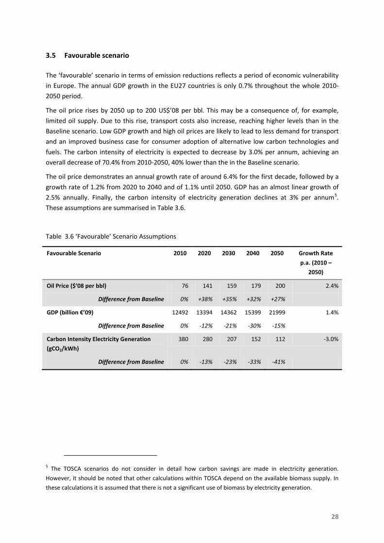
4.3 Aggregated Scenario Results .....................................................................................................37
Growth rates by scenario and mode of transport .......................................................................... 37
Total passenger and freight transport by scenario ......................................................................... 40
4.4 Detailed scenario results ............................................................................................................41
Baseline scenario results ................................................................................................................. 41
Challenging scenario results ............................................................................................................ 43
Favourable scenario results ............................................................................................................ 44
4.5 Conclusions .................................................................................................................................46
5 References ...................................................................................................................... 48
Annex A: Sensitivity Analysis - Disruptive Scenario ....................................................................... 53
Assumptions ...........................................................................................................................................53
Sensitivity analysis results ......................................................................................................................56
Conclusions .............................................................................................................................................59

5
Abbreviations
Abbreviation Description
AIM Aviation Integrated Modelling
bpkm Billion passenger kilometre
btkm Billion tonne kilometre
CO2 Carbon dioxide
eg. exempli gratia – for example
Eq. equation
etc. et cetera – and the rest
GDP Gross Domestic Product
GHG Greenhouse Gas
iTREN Integrated transport and energy
Mtoe Million tonnes of oil equivalents
Mton Million tonnes
pkm Passenger kilometre
SULTAN SUstainabLe TrANsport
tkm Tonne kilometre
TOSCA Technology Opportunities and Strategies toward Climate-friendly trAnsport
Transtools TOOLS for TRansport Forecasting ANd Scenario testing
TTW Tank-to-Wheels (downstream emissions, direct emissions)
WTT Well-to-Tank (upstream emissions, indirect emissions)
WTW Well-to-Wheels (fuel lifecycle emissions) = WTT+TTW

6
Abstract
The TOSCA project aims to identify promising technology and fuel pathways to reduce
transportation-related greenhouse gas emissions through mid-century. An important building block
of this project is the techno-economic specification of low-GHG emission transportation
technologies, which are input into a scenario analysis. TOSCA considers all major modes of passenger
and freight transport, along with transportation fuels and technologies capable of enhancing
infrastructure capacity. This report is thus one out of a number of such techno-economic studies.
TOSCA Work Package 6 (WP6) integrates the technology, fuel, and infrastructure studies carried out
in WP1-5 through a scenario and modelling analysis. The first step in the scenario analysis consisted
of a systematic review of existing European transport scenarios. Consequently, we determined a set
of scenario variables that affect future passenger and freight transport demand. These are used to
formulate four distinct scenarios (three detailed scenarios and one sensitivity case) that describe the
future levels of passenger and freight transport demand. The modelling stage includes the projection
of transport demand for each scenario under the assumption of no new policies. This part of the
modelling stage was carried out with the EU demand model Transtools (JRC, 2010). Due to the
limitations of that model, we complemented the Transtools model with other models such as the
Aviation Integrated Model (AIM). This report (WP 6.1) details the scenario generation and demand
modelling steps described above. A further report (WP6.2) investigates the fleet composition and
emissions which would result in each of these scenarios.
7
1 Introduction
1.1 Background
In December 2008, in order to combat climate change and increase the EU’s energy security, the
European Union adopted a climate and energy package. This package (‘3x20%’) includes the
following emissions and energy use reduction targets to be met by 2020:
• A reduction in EU GHG emissions of at least 20% below 1990 levels
• 20% of EU energy consumption to come from renewable resources
• A 20% reduction in primary energy use compared with projected levels, to be achieved by
improving energy efficiency.
EU Member States agreed to realise the emission reduction target (EC, 2008b) by the following
actions:
• A revision and strengthening of the Emissions Trading System (EU ETS) that sets a single EU-
wide cap on emission allowances. This cap will be cut annually, reducing the number of
emission allowances available to businesses by 21% below the 2005 level in 2020.
• An 'Effort Sharing Decision’ governing emissions from sectors, such as transport, housing,
agriculture and waste that are not covered by the EU ETS. Under this decision each Member
State has agreed to a binding national emissions limitation target for 2020 which reflects its
relative wealth. These national targets will cut the EU’s overall emissions from the non-ETS
sectors by 10% by 2020 compared with 2005 levels.
• The 10% reduction from the effort sharing decision, together with the 21% reduction from
the EU ETS during the same period, will accomplish the overall emission reduction goal of the
EU Climate and Energy package (20% cut below 1990 levels by 2020).
The transport sector, being strongly interconnected with many other sectors, currently accounts for
around 25% of EU27 GHG emissions and this share is increasing (EC 2010a), so changes in the
transport sector will be vital in achieving EU targets for total emissions. Thus, thorough planning
toward climate-friendly transport is fundamental. Before proceeding to the main subject of this
document, which is a discussion of the scenario generation process for the Technology Opportunities
and Strategies toward Climate-friendly trAnsport (TOSCA) project, a short description of the
transport sector is provided regarding the elements which are emphasized in the scenario analysis.
1.2 Macro-economic transport-related trends in Europe
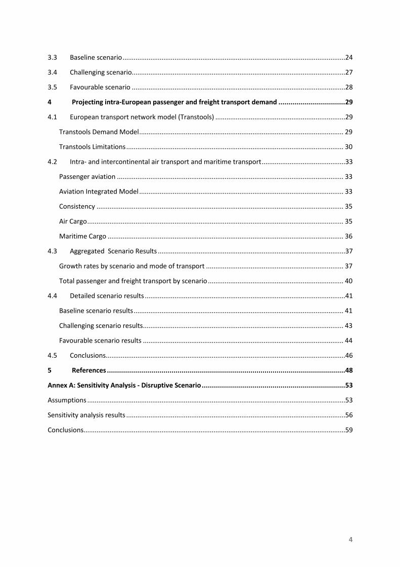
Figure 1.1 depicts Final Energy Consumption in the EU27 countries to 2007, in Mtoe. One can clearly
observe that transport is one of the highest-consumption sectors (with a percentage of 32.6% for
2007). By 2000 transport energy consumption surpassed that of the industry sector (27.9% in 2007).
Accounting for almost one third of total energy consumption, transport is a strong driver for the
definition of current and future EU policies.
8
Figure 1.1 Final EU27 Energy Consumption by Sector
CO2 Emissions* by Sector: EU-27
0,70
0,80
0,90
1,00
1,10
1,20
1,30
1990
1991
1992
1993
1994
1995
1996
1997
1998
1999
2000
2001
2002
2003
2004
2005
2006
2007
1990=1
Energy Industries Industry ***Transport ** ResidentialCommercial / Institutional Other ****Total
Source: EU Energy in Figures 2010 DG TREN (EC, 2010a)
* Excluding LULUCF (Land Use, Land – Use Change and Forestry) Emissions and International Bunkers
** Excluding International Bunkers (international traffic departing from the EU)
*** Emissions from Manufacturing and Construction and Industrial Processes
**** Emissions from Fuel Combustion in Agriculture/Forestry/Fisheries, Other (Not elsewhere specified), Fugitive Emissions
from Fuels, Solvent and Other Product Use, Waste, Other
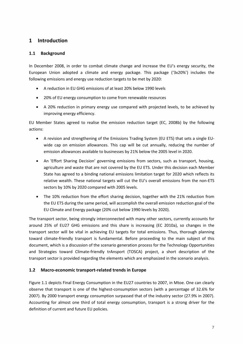
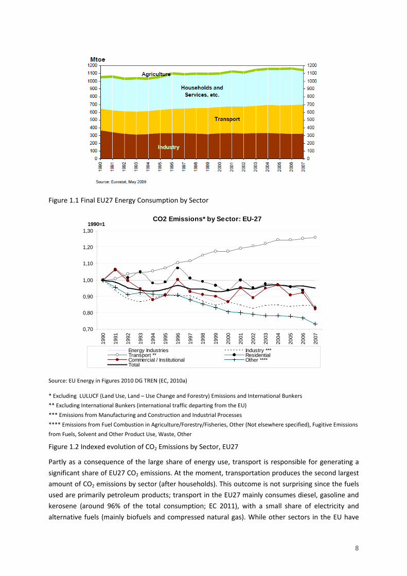
Figure 1.2 Indexed evolution of CO2 Emissions by Sector, EU27
Partly as a consequence of the large share of energy use, transport is responsible for generating a
significant share of EU27 CO2 emissions. At the moment, transportation produces the second largest
amount of CO2 emissions by sector (after households). This outcome is not surprising since the fuels
used are primarily petroleum products; transport in the EU27 mainly consumes diesel, gasoline and
kerosene (around 96% of the total consumption; EC 2011), with a small share of electricity and
alternative fuels (mainly biofuels and compressed natural gas). While other sectors in the EU have

9
shown a decreasing trend in CO2 emissions since 1990, transport continues to emit more carbon
dioxide (Figure 1.2).
Within the transport sector, civil aviation (domestic including international bunkers) shows the
largest growth in CO2 emissions since 1990 (Figure 1.3). However, road and shipping emissions have
also been increasing.
CO2 Emissions* from Transport, EU-27
0,500,600,700,800,901,001,101,201,301,401,501,601,701,801,90
1990 1991 1992 1993 1994 1995 1996 1997 1998 1999 2000 2001 2002 2003 2004 2005 2006
1990=1
Civil Aviation Road Railw ays
Navigation Other Total
Source: EU Energy in Figures 2010 DG TREN (EC, 2010a)
* Excluding LULUCF (Land Use, Land – Use Change and Forestry) Emissions and International Bunkers
Figure 1.3 Indexed evolution of CO2 emissions by transport mode, EU27
The increase in transport sector CO2 emissions is strongly linked to economic growth. Figure 1.4
illustrates the link between socio-economic trends (GDP and population) and the volume of transport
(passenger and freight), and consequently the resulting transport GHG emissions. Economic growth
is a general trigger for transport demand because it means more goods are produced and
transported and people have more income available for transportation. This means that reducing
transport CO2 emissions will require either decoupling transport demand from economic growth,
decoupling transport demand from carbon atoms that are oxidized to CO2. TOSCA looks primarily at
the second of these options.
Although the TOSCA project has the goal of investigating how greenhouse gas emissions can be
reduced by new vehicle and fuel technologies, the likely future adoption and impact of these
technologies is fundamentally dependent on the future development of various exogenous factors.
For example, in a future world with low oil prices, the demand for energy efficient low carbon
technologies and fuels will be lower than in a future world with high oil prices. The high uncertainty
attached to future projections of these exogenous factors makes a scenario-based analysis
considering multiple different futures vital.

10
Source: EU energy and transport in figures (EC, 2009c)
Figure 1.4 Indexed evolution of GDP, population and GHG emissions from freight and passenger
transport demand
WP1:Road
WP2: Air
WP3: Rail
Marine
WP1:Road
WP2: Air
WP3: Rail
Marine
WP4: Fuels
WP5: Capacity
WP6/7:Modelling
WP7:Future Policies
WP6: Future Scenarios
Promising Technology/Policy combinations for reducing EU GHG Emissions to 2050
Figure 1.5 TOSCA Work Package structure
1.3 The TOSCA Project
The TOSCA project is an EU FP7 project investigating the potential of alternative vehicle technologies
to reduce the environmental impact of EU27 transportation to 2050. The structure of the project is
shown in Figure 1.5. Initially, WP1-5 estimate the techno-economic characteristics of current and
future vehicle, fuel and infrastructure technologies. WP6 then integrates these study results with
transport demand projections through a scenario and modelling analysis. The first step in the
scenario analysis consisted of a systematic review of already existing European transport scenarios.
Consequently, we determined a set of scenario variables that affect future passenger and freight
transport demand. These are then used to formulate four distinct scenarios (three detailed scenarios
and one sensitivity case) that describe the future levels of passenger and freight transport demand.
The modelling stage includes the projection of transport demand for each scenario under the
assumption of no new policies. This part of the modelling stage was carried out with the EU demand

11
model Transtools (JRC, 2010). Due to the limitations of that model, we complemented the Transtools
model with other models such as the Aviation Integrated Model (AIM). This report (WP 6.1) covers
the scenario analysis and demand modelling stages. A further report (WP6.2) covers technology
uptake and CO2 emissions by scenario.
The basic structure of the TOSCA modelling block is shown in Figure 1.6. In addition to the exogenous
factors (growth in GDP, oil price, and the CO2 intensity of electricity) which form part of the TOSCA
scenarios, the modelling stage uses several other major inputs. These include an updated form of the
European Transport Policy Information System (ETIS), which forms the input to the Transtools model.
This database contains a wide range of transport policy-relevant variables, as appropriate for a 2005
base year (NEA, 2005). TOSCA input consists of changes to the Transtools input database to reflect
the development of baseline scenario variables from 2005 for each year run (e.g. in terms of
population, urbanisation, fuel prices, carbon prices) and any development in the characteristics of
the reference technologies identified by WP 1-5 (e.g. in terms of cost, speed and fuel consumption).
In the case that the database contains a cost to end-users rather than operators (for example, rail
ticket prices rather than costs accruing to rail operators) it is assumed that all cost increases are
passed on to consumers.
Demand, fleet and emissions
Technology Characteristics
Demand Modelling
(Trantools/AIM)
PolicyCharacteristics
ScenarioCharacteristics
Reference only
Stock Model
Changes in Demand(Summa)
All technologies
Promising Technology/Policy combinations for reducing EU GHG Emissions to 2050
Figure 1.6 TOSCA Modelling approach
The remainder of this document is structured as follows. Chapter 2 presents a review of existing
transport scenarios for the EU. Chapter 3 outlines the framework for both passenger and freight
transport that is used to construct and evaluate the TOSCA scenarios. It describes the steps leading
to the definition of the scenarios, and describes a baseline and two internally consistent alternative
scenarios including the underlying assumptions. The scenarios are based on the most relevant and
uncertain exogenous drivers with a potentially large impact on the primary outcome-of-interest, GHG
emissions reductions in transport. Chapter 4 describes the projected demand for transport and
12
modal split by scenario. Finally, in the annex we discuss the effects that a disruptive event may have
on transport demand, and give results from a sample disruptive scenario.
2 Review of existing transport scenarios for Europe
Many scenarios for future EU27 transport demand already exist. Within the scope of this work
package a large number of studies, models and data sources have been reviewed. The review focuses
on quantified transport and energy scenarios, both ‘Baseline’ (no or limited emissions mitigation
policies) and decarbonisation or GHG mitigation scenarios. In analyzing the various studies, the
scope, underlying assumptions and the evolution of key system variables or outputs of the scenarios
were compared. Specifically, the main aspects considered for this review were:
• Timeframe of the scenarios, including a horizon up to 2030 or 2050.
• Geographical scope, including the EU27 or other regions.
• Scope of the transport sector, including all modes or only selected modes.
• Volume of transport, including explicit demand modelling or not.
• Scope of the emissions, including tank-to-wheel (TTW) emissions or well-to-wheel (WTW)
emissions.
• Definition of a scenario, including exogenous drivers, policy instruments or both.
• Key assumptions including GDP per capita, oil prices, and other drivers.
• Nature of the scenario drivers (e.g. linear/continuous or disruptive).
A representative selection of these scenario exercises are reviewed and described individually below.
2.1 EU transport GHG: routes to 2050
Description
The SULTAN Illustrative Scenarios Tool was developed as part of the EU Transport GHG: Routes to
2050? Project (Hill et al, 2010). The project as a whole reviewed the abatement options – technical
and non-technical – that could contribute to reducing transport’s greenhouse gas (GHG, WTW scope)
emissions, both up to 2020 and in the period from 2020 to 2050. SULTAN is a Microsoft Excel-based
tool that can be used to investigate GHG emissions, and some other outputs, associated with
transport from the EU-27 countries in the period 2010-2050. It allows users to create and edit “Policy
Scenarios” – illustrative scenarios for the EU transport system that make assumptions on how
policies might impact on the transport system – and then view the outcomes of the scenarios in
terms of GHG emissions, some other pollutant emissions and some abatement costs. The SULTAN

13
tool is a high-level scoping tool for quick appraisals, not for detailed transport policy impact
assessments.
Results
The baseline scenario shows that the total transport GHG emissions may increase from about 1,600
Mton CO2 equivalent emissions in 2010 to more than 2,000 by 2050. The combined reduction
potential from selected technical and non-technical abatement measures indicates that a reduction
of up to 80-90% over the 1990 level in total transport GHG emissions could be achieved by 2050.
2.2 TRANSvisions
Description
TRANSvisions (2009a) discusses a wide range of drivers related to transport. Three main categories
were identified. First, external drivers, that is, drivers external to the transport sector, for which five
main categories were identified (population, economic development, energy, technology
development and social change). Second, internal drivers, that is, drivers internal to the transport
sector, e.g., infrastructure, vehicles and fuel development and transport impact on environment and
society. Finally, policy drivers, that is, broad policy responses which affect the evolution of the
transport system, and in particular the governance of the transport sector.
A number of different exploratory scenarios for 2050 were formulated based on the identified
drivers. Each scenario was formulated as a different path towards a post-carbon society. A “meta-
model” was developed for the scenario analysis for the timeframe 2005-2050. The meta-model
applied in TRANSvisions was calibrated against scenario results from the Eurpean Commission’s
transport model Transtools for 2005 and 2030. The Transtools scenarios are established based on the
main inputs for the Transtools model. Such inputs include: socio-economic input (population, GDP
development, work places); transport policy input (change in vehicle operating costs, fares and
transport costs for different transport modes); and network input (links and nodes and data related
to these). Four main scenarios were evaluated:
1. The behavioural path: “Moving Less” or Reduced Mobility: Environmental concern and
changes in behaviour.
2. The technological path: “Moving Alone” or Induced Mobility: Exponential growth of
technological improvements, unlimited clean and cheap energy sources, high economic
growth.
3. The mandatory path: “Stop Moving” or Constrained Mobility: Very slow process of
technological implementation, high pensions and health cost, low productivity, strong
mobility regulation, legislation and taxation.

14
4. The organisational path: “Moving Together” or Decoupled Mobility: Strong decoupling
between economic development and growth of traffic volume is gradually achieved, changes
in behaviour.
Results
As both exogenous drivers like GDP per capita and policy assumptions like taxation are used, as well
as ‘wildcard’-type assumptions such as unlimited clean and cheap energy, the resulting demand for
transport varies considerably across the scenarios. Due to different levels of carbon intensity in each
of the scenarios, the resulting CO2 emissions show a smaller range around the baseline. The results in
terms of CO2 emissions trajectories to 2050 show that in all scenarios at least a 10% reduction in
emissions might be achieved by 2050 compared to 2005. The scenarios Decoupled and Reduced
Mobility might achieve over a 50% reduction in emissions by 2050 compared to 2005.
2.3 iTREN2030 Integrated transport and energy baseline
Description
The iTREN-2030 (iTREN, 2009) project contributes to the extension of the European policy
assessment toolbox providing improved tools as well as a consistent energy and transport baseline
scenario, called the Reference scenario, for the EU to 2030. iTREN-2030 applies updated versions of
four European models to generate the baseline scenario:
1. ASTRA (2000), an integrated and strategic transport-economy assessment model.
2. POLES (2006), a global energy model describing the supply- and demand-side of world
energy markets from a technological bottom-up perspective.
3. Transtools, a European transport model focusing on the medium- to long distance transport
flows on the European transport networks.
4. TREMOVE (2007), an environmental assessment model providing vehicle fleet, fuel
consumption and emission indicators for the European transport system.
The basic concept of the Reference scenario is “frozen policy 2008”, i.e. the scenario considers only
policies that were decided by the EU Council and/or EU parliament by mid 2008. It should be noted
that the global economic crisis that started in 2008 is not reflected in the iTREN-2030 Reference
scenario. The iTREN-2030 Reference scenario shows that transport demand will increase until 2030,
especially freight demand, which is projected to be 50% larger in the year 2030 than in the year
2005, while passenger demand is expected to grow more slowly. Therefore, for the EU27 as a whole,
some relative decoupling between economic growth and transport demand is expected, only for
passengers but not for freight. While the economy of the EU27 is expected to grow on average at
1.5% per year until 2030 (but with a decreasing level of employment), and transport increases at a
slightly lower rate, final energy demand is expected to grow less than 1% per year, which means that
the EU27 should become slightly more energy-efficient (iTREN, 2009).

15
Results
The Reference scenario developed in the iTREN-2030 project shows that transport CO2 emissions are
expected to increase from 1,268 million tons in 2005 to 1,485 million tonnes by 2030, an increase of
17% or 0.6% annually. Oil prices are expected to more than double between 2005 and 2030 from 44
to 90 € 2005 per barrel.
2.4 EU energy trends to 2030 (Primes 2009 baseline)
Description
PRIMES (PRIMES, 2010) is a general purpose energy system model supported by some more
specialised models, such as the GEM-E3 and PROMETHEUS. The GEM-E3 (World and Europe versions)
model is an applied general equilibrium model, simultaneously representing 37 World regions/24
European countries, which provides details on the macro-economy and its interaction with the
environment and the energy system. It covers all production sectors (aggregated to 26) and
institutional agents of the economy. GEM-E3 is specifically designed to provide high resolution
output by energy sector and GHG emission source (E3M-Lab, GEM-E3 model description). A fully
stochastic World energy model is used for assessing the uncertainties and risks associated with the
main energy aggregates including uncertainties associated with the impact of policy actions (R&D on
specific technologies, taxes, standards, subsidies and other supports). The model makes endogenous
projections of future energy prices, supply, demand and emissions for 10 World regions (E3M-Lab
PROMETHEUS model description).
Primes is designed for future projections, scenario building and policy impact analysis. It covers a
medium to long-term horizon to 2030. The PRIMES model simulates a market equilibrium solution
for energy demand and supply. It includes transport activity for both passengers and freight. The
model structure defines several technology types (car technology types, for example), which
correspond to the level of energy use. Within road transport, a further subdivision distinguishes
between public road transport, motorcycles and private cars. The model considers six to ten
alternative technologies for transport means such as cars, busses and trucks; the number of
alternatives is more limited for rail, air and navigation (PRIMES, 2010).
The “EU energy trends to 2030” study (E3M-Lab, 2009) is an update of previous trend scenarios, such
as the “European energy and transport - Trends to 2030” study published in 2003 and its 2005 and
2007 updates. Two scenarios, the “Baseline 2009” (finalised in December 2009) and the “Reference
scenario” (April 2010) are presented. The scenarios are available for the EU and each of its 27
Member States simulating energy balances for future years under current trends and policies as
implemented in the Member States by April 2009.
The Baseline 2009 scenario determines the development of the EU energy system under current
trends and policies; it includes current trends in population and economic development including the
recent economic downturn and takes into account the highly volatile energy import price
environment of recent years. Economic decisions are driven by market forces and technology

16
progress in the framework of concrete national and EU policies. Measures implemented before April
2009 are included. This includes the EU emissions trading scheme (ETS) and several measures for
energy efficiency but excludes the renewable energy target and the non-ETS targets. The Reference
scenario is based on the same macroeconomic conditions, price, technology and policy assumptions
as the baseline. In addition to the measures reflected in the baseline, it includes policies adopted
between April and December 2009 and assumes that national targets under the Renewables
directive 2009/28/EC and the GHG Effort sharing decision 2009/406/EC are achieved in 2020.
Results
Key assumptions for the 2009 Reference scenario include:
• a GDP growth rate of 2.2% annually between 2010 and 2020 and 1.7% between 2020 and
2030;
• Rising oil price to about 106 US$ 2008 per barrel by 2030;
• A decreasing carbon intensity of power generation to 179 grams CO2 per kWh by 2030;
• Increasing average after tax electricity prices from 110 to 144 €2005 per MWh between 2010
and 2030.
The total CO2 emissions from transport (excluding maritime and intercontinental aviation) in the
Reference scenario remain at about 1,000 to 1,100 million tonnes of CO2 between 2010 and 2030.
2.5 Roads toward a low carbon future
Description
The background of the study (McKinsey, 2009) is the increasing policy focus on carbon dioxide
emissions from passenger vehicles, due to the fact that these vehicles are a highly visible source of
greenhouse gases and total passenger vehicle emissions are projected to grow to 2030. Three
scenarios are defined assuming different rates and time frames for the diffusion of different
technology packages. These scenarios are:
• ICE scenario
This scenario assumes optimization of the fuel efficiency of ICE-powered vehicles. The sector
does not witness any meaningful global penetration of hybrid or electric vehicles.
• Mixed-technology scenario
A balanced mix of technological solutions reaches the market, including optimized ICEs,
hybrids, and electric vehicles.
• Hybrid-and-electric scenario
There is a rapid transition toward a world of electricity-based vehicle propulsion systems.

17
Results
The CO2 abatement curve that was constructed for Europe in this study includes a number of
abatement options ordered with increasing cost per tonne of CO2. The x-axis represents cost-
effectiveness levels at an oil price of US$ 60 WTI (West Texas Intermediate) or 45€. In addition, two
other dashed horizontal lines represent cost-effective abatement levels at oil prices of 100 (or 75€)
and 150 US$ (or around 110€) per barrel. The results show that over 200 million tons of CO2
equivalent emissions can be abated by abatement options at negative marginal abatement costs
assuming a 60 US$ per barrel oil price.
2.6 Transport, Energy and CO2 scenarios
Description
This study (IEA, 2009) shows how the introduction and widespread adoption of new vehicle
technologies and fuels, along with some shifting in passenger and freight transport to more efficient
modes, could result in a 40% reduction in CO2 emissions below year-2005 levels. This analysis uses
the same basic set of scenarios originally developed for the Energy Technology Perspectives (ETP,
2008) publication. These cover various futures through 2050, including several alternative routes to
achieve very low CO2 emissions for transport. Specific scenarios include:
• Baseline: follows the IEA World Energy Outlook 2008 (WEO 2008) Reference Case to 2030
and then extends it to 2050. It reflects current and expected future trends in the absence of
new policies.
• High Baseline: considers the possibility of higher growth rates in car ownership, aviation and
freight travel over the period to 2050 than occur in the Baseline.
• BLUE CO2 reduction scenarios: these scenarios update those presented in the IEA Energy
Technology Perspectives 2008 report. The BLUE variant scenarios are developed based on
achieving the maximum CO2 reductions achievable from transport by 2050 using measures
costing up to USD 200 per tonne of CO2. These scenarios will require significant policy
intervention if they are to be achieved.
• BLUE Map: this scenario achieves CO2 emissions by 2050 that are 30% below 2005 levels. It
does this via improvements in vehicle efficiency and the introduction of advanced
technologies and fuels such as plug-in hybrids (PHEVs), electric vehicles (EVs), and fuel cell
vehicles (FCVs). It does not envisage significant changes in travel patterns.
• BLUE EV Success: Similar to BLUE Map and achieving a similar CO2 reduction, but with electric
and plug-in hybrid vehicles achieving greater cost reductions and better performance to the
point where they dominate light-duty vehicle (LDV) sales by 2050, to the exclusion of fuel cell
vehicles.

18
• BLUE Shifts: this scenario focuses on the potential of modal shift to cut energy use and CO2
emissions. Air and LDV travel grow by 25% less than in the Baseline to 2050, and trucking by
50% less. The travel is shifted to more efficient modes and (for passenger travel) to some
extent eliminated via better land-use planning, greater use of information technology, and
other measures that reduce the need for motorised travel. Compared to the Baseline in
2050, BLUE Shifts results in a 20% reduction in energy use and CO2.
• BLUE Map/Shifts: this scenario combines the BLUE Map and BLUE Shifts scenarios, gaining
CO2 reductions from efficiency improvements, new vehicle and fuel technologies, and modal
shift. It results in a 40% reduction in CO2 below 2005 levels by 2050.
Results
The oil price is assumed to remain at 120 US$ per barrel from 2030 to 2050 in 2006 real US$. In
nominal prices this means the oil price will increase to over US$ 300 per barrel by 2050. In the
baseline for OECD Europe transport GHG emissions are expected to remain at the 2005 level of about
1,500 Mton CO2 eq. to 2050. Worldwide transport sector GHG emissions in the BLUE Map/Shifts
scenarios are 40% below year-2005 levels.
2.7 Findings from scenario review
• Based on the review of scenarios in this chapter, which are summarised in Table 2.1 below,
we draw the following conclusions:
• Scenario timeframes vary:
O Some studies focus on the end results by 2030 or 2050, while others focus on the
trajectory to the time horizon as well.
• Geographical scope varies:
O Some studies include the EU27, whereas others include world regions, OECD areas or
Western Europe only.
• The investigated scope of the transport sector varies:
o Some studies include all modes; others include selected modes.
o Some studies include main transport corridors/network; others include the full
transport network.
• The volume of transport varies:
o Some studies include explicit demand modelling, others do not. In the latter case,
fixed demand assumptions are applied in all scenarios.
• The scope of emissions varies:
o Some studies include only TTW emissions, where others include WTW emissions.

19
• The definition of a scenario varies:
o Some studies include only exogenous drivers (external forces), while others include
policy instruments or both.
• Key determinants vary:
o Some studies include only GDP and population, whereas others include oil prices and
other variables.
o Few studies include the carbon intensity of electricity as a scenario variable for
transport scenarios.
• The nature of the scenarios varies:
o Most scenarios are linear/ continuous (growth rate extrapolations).
o Few scenarios include disruptive developments/events.
Table 2.1 Review of existing transport scenarios
Scenario exercise:
Review element:
Hill et al., 2010
TRANSvisions, 2009a
iTREN, 2009 E3M-Lab, 2009
McKinsey, 2009
IEA, 2009
Timeframe 2050 2030 and 2050
2030 2030 2030 2050
Geographical scope
EU27 EU27 EU27 EU27 Europe World region, OECD Europe
Transport sector scope
All modes All modes (only intra-EU)
All modes (only intra-EU)
All modes (only intra-EU)
Passenger vehicles
All modes
Transport demand scope
No demand modelling, fixed assumption
Demand modelling
Demand modelling
No demand modelling, fixed assumption
No demand modelling, fixed assumption
No demand modelling, fixed assumption
Scope of emissions
WTW WTW Not specified Not specified WTW WTW
Scenario definition
Policy scenarios (technical and non-technical)
Exogenous and policy scenarios (mixed)
Baseline exogenous and policy assumptions (mixed)
Baseline exogenous and policy assumptions (mixed)
Policy assumptions (abatement options)
Policy assumptions (transport system assumptions)
Nature of scenarios
Continuous Continuous Continuous Continuous Continuous Continuous
Key assumptions
Based on TREMOVE, ExTremis, MARKAL-ED
Based on Transtools (metamodel)
Based on Transtools, TREMOVE, POLES, ASTRA
Based on Primes energy baseline 2009
Based on Global GHG abatement cost curve v2.0
Based on Mobility Model (MoMo)

20
In combination, these factors mean that it can be difficult to compare the results and projected
reductions in emissions from different scenario studies. For example, a study on a scope which
includes only emissions sources which have a relatively large range of mitigation options (e.g.
passenger cars) will project greater reduction potentials than one which includes sources which have
fewer options (e.g. intercontinental aviation). Based on the observations made in this review, the
next chapter clearly defines the approach used in TOSCA for the scenario formulation.

21
3 Scenario formulation
3.1 Definition of a TOSCA scenario
As mentioned in section 2, many scenario exercises use a mix of policy instrument and exogenous
factors to define scenarios. In TOSCA scenarios are defined as follows:
• Scenarios include exogenous variables only
• These exogenous variables are both uncertain and relevant for reducing GHG emissions
• The scenarios include a set of consistent assumptions about the future development of these
variables
• The scenarios are not forecasts, but represent a range of plausible futures
• The scenarios are intended to describe the uncertainty about the future collection of
consistent assumptions
3.2 Identification of scenario drivers
In TOSCA we focus exclusively on exogenous scenario drivers. A framework is used to select variables
that are both relevant and uncertain in terms of reducing GHG from transport. Relevant and
uncertain variables form one block of the evaluation framework used in this project (Table 3.1).
Variables having a low relevance are ignored. Variables which are relevant but not highly uncertain
are included in the Baseline scenario. The Baseline scenario is the reference development used to
evaluate the impact of alternative exogenous scenario developments. Variables with a high relevance
and high uncertainty are used as key scenario variables for the definition of the TOSCA scenarios. The
variables with the highest relevance and largest uncertainty include oil prices (and other energy
prices as a derivative of oil prices), GDP growth and the carbon intensity of electricity generation. The
reasons for these choices are described below.
EU transport depends on oil products for 96% of its energy needs. Transport accounts for 73% of all
oil consumed in Europe (EC, 2011). Oil prices depend on many factors, which are difficult to predict.
Oil prices generally have a large impact on the total volume of passenger and freight transport and
on mode/technology choices. Higher oil prices improve the business case of low carbon alternative
technologies and fuels.
Economic growth, measured as GDP, is another important driver of the volume of transport. Lower
economic growth (or an economic crisis) leads to lower transport demand, which may require less
stringent policy measures for reducing GHG emissions to a certain desired level. In addition, lower
economic growth may also lead to different fuel/technology choices by transport users. Similar
responses are found in certain transport service operations like in shipping; reduced demand for
consumer goods leads to a lower volume of freight transport which leads to overcapacity in (for
instance) container shipping. In response to this, shippers implement slow steaming, leading to
longer voyages (in days) but lower emissions.

22
Table 3.1 Evaluation framework for selecting exogenous drivers in TOSCA.
Uncertainty about development
Low High
Rele
vanc
e fo
r EU
27 G
HG
em
issi
on r
educ
tion
Low IGNORE
IGNORE
High Include on baseline: - Aging population - Population size - Urbanisation - Motorisation rate
Exogenous drivers: - Oil prices - Economic growth (GDP) - Carbon intensity of electricity
The carbon intensity of electricity generation is defined as the amount of CO2 equivalent emissions
per kilowatt hour (kWh) electricity generation (gram CO2 per kWh). This variable will become highly
relevant to transport as many future projections include electricity becoming a significant energy
source for EU transport (via plug-in hybrids, battery electric vehicles or a mode shift to rail). If
transport becomes highly electrified, but electricity does not improve considerably in terms of
carbon intensity, EU transport may not be able to significantly reduce its emissions.
Based on our review of a long-list of existing transport scenarios and models, of which a selection is
presented in chapter 2, we formulated a set of scenarios which include a wide range of the evolution
of the three scenario drivers. The table below depicts four scenarios. The first three scenarios are
defined as follows:
• A reference for the evolution of exogenous factors (Baseline)
• Challenging evolution of exogenous factors in terms of GHG emissions (Challenging)
• Favourable evolution of exogenous factors in terms of GHG emissions (Favourable)
Table 3.2 Overview of the key scenario assumptions which define the three TOSCA scenarios
Scenario assumptions:
Oil prices (US$2008/bbl)
GDP (p.a. % growth)
Carbon intensity (p.a. % growth)
Scenario 0: ‘Baseline’ Increasing 76 to 157 (+1.8%)
Increasing +1.7%
Decreasing -1.7%
Scenario 1: ‘Challenging’
- 76 to 76 (0%)
+ + +2.5 %
+ -0.5%
Scenario 2: ‘Favourable’
+ 76 to 200 (+2.5%)
- +0.7%
- - -3.0%
Scenario 3: ‘Disruptive’ (Annex A)
0 76 to 157 (+1.8%)
0 +1.7%
0 -1.7%

23
0
50
100
150
200
250
1850 1870 1890 1910 1930 1950 1970 1990 2010 2030 2050
Oil
Pric
es U
SD'0
8 pe
r bar
rel
BP Historic Prices Scenario 0: 'Baseline'
Scenario1: 'Challenging' Scenario 2: 'Favourable'
Figure 3.1 Assumptions for Oil prices in all scenarios
The fourth scenario, Disruptive, mainly functions as a sensitivity analysis. The disruptive scenario
explores the behaviour of the TOSCA framework conditions under the occurrence of an extreme
event in the year 2020 (see Annex A). The development of the identified drivers for the other
scenarios is described below. The assumptions as mentioned in the table above are shown in the
following graphs. In the following sections, each scenario is described in detail. Figure 3.1 above
shows the historic development of yearly average oil prices from 1861 to 2009 and three alternative
oil price scenarios from 2009 to 2050.
0
5000
10000
15000
20000
25000
30000
35000
40000
1990 2000 2010 2020 2030 2040 2050
EU27
GD
P in
bill
ion
EUR
'09
Scenario 0: 'Baseline' Scenario 1: 'Challenging'
Scenario 2: 'Favourable' Eurostat
Figure 3.2 Assumptions for GDP in all scenarios

24
Figure 3.2 shows the historic development of GDP in the EU27 from 1990 to 2005 and the three
alternative GDP scenarios from 2009 to 2050.
0
200
400
600
800
1000
1200
1960 1970 1980 1990 2000 2010 2020 2030 2040 2050
Car
bon
Inte
nsity
g C
O 2 /
kWh
World energy balances (IEA, 2010) and Emission Factors (ETC/ACC, 2003)Scenario 0: 'Baseline' Scenario 1: 'Challenging'Scenario 2: 'Favourable'
Figure 3.3 Assumptions for Carbon Intensity of electricity generation in all scenarios
Figure 3.3 above shows the historic development of the carbon intensity of electricity generation in
the EU27 from 1960 to 2007 and the three alternative carbon intensity scenarios from 2009 to 2050.
3.3 Baseline scenario
The Baseline scenario assumes a continuation of the existing socio-economic trends for EU transport
demand drivers. It is assumed that current policies1
will be successfully implemented and that no
other significantly different policies are introduced. In this scenario, as for all scenarios, the EU is
committed to reduce total GHG emissions by at least 20% relative to the 1990 level by 2020, as
specified in COM (2007), with a further tightening beyond 2020. Table 3.3 presents the evolution of
the relevant and uncertain scenario drivers and baseline variables which are relevant and less
uncertain.
1 This includes, for example, maintaining existing levels of fuel excise duty and VAT, and including aviation in
the EU emissions trading scheme from 2012.

25
Table 3.3 ‘Baseline’ scenario drivers and baseline variables
Scenario 0: ‘Baseline’ Unit 2010 2020 2030 2040 2050 Growth Rate
2010-2050
Relevant and uncertain scenario drivers:
Oil price US$ per bbl, 2008
76 102 118 136 157 1,8%
Carbon intensity electricity generation (DBFZ forecast /EURelectric)
g CO2 / kWh 380 262 145 117 89 -3,6%
GDP EU27 Billion €, 2009
12811 15747 18621 21999 25965 1,8%
GDP per Capita, EU27 €, 2009 PPP2 25674 30636 35810 42510 50417 1,7% Relevant and low-uncertainty baseline variables:
Population size EU27 Million, EU27 499 514 520 518 515 0,1% Urbanisation (EU27) Million, EU27 369 392 413 426 438 0,4% Urbanisation Rate (EU27) % 74 76 79 82 85 0,3% Motorisation rate (EU27) cars/1000
inhabitants 451 512 566 626 692 1,1%
Electricity prices € 2009/MWh 118 150 155 151 147 0,5%
Oil prices3 are shown in figure 3.1. This graph depicts the development of crude oil prices from BP
since 1861. One can here observe the price fluctuations which contribute to the high uncertainty in
the future development of this variable4
. From 2010 on, these prices steadily increase in the baseline
scenario with an average annual growth rate of 1.8%. By 2020 oil price is expected to rise beyond
100 US$’08 per barrel, originally due to growing demand but, later on, also because of being a finite
resource. Gas prices are assumed to be highly positively correlated to oil prices.
GDP growth is expected to increase moderately in the EU27 to 2050. The average EU27 growth rate
for GDP in the baseline scenario is projected to be 1.8% per annum for the EU27 countries (Table
3.3). GDP per capita demonstrates a slightly smaller growth rate of 1.7% per annum, due to a small
growth in population.
2 Note that some of the models within TOSCA used require input in the form of market exchange rate (MER)
GDP. In this case, the study of Manne, Richels & Edmonds (2005) was used to provide a plausible conversion
factor.
3 Oil prices affect transport costs. The effect though may be limited as a high proportion of gasoline and diesel
price is tax which is assumed to remain at present-day levels. In addition, for some transport modes energy
costs represent only a low proportion of operating costs (e.g. around 10% for rail).
4 Some of the main influencing factors of the oil price are economic growth, car ownership and in general fuel
demand, the existing –known and unknown- fuel reserves and the producing countries’ relationships to the
rest of the world.

26
The carbon intensity of electricity is projected to decrease due to cleaner, more efficient electricity
generation techniques and different primary energy sources. This expected technological evolution,
combined with the EU ETS regulation applicable to stationary emission sources such as power plants,
is projected to reduce the carbon intensity of electricity generation by 3.6% annually from 2010 to
2050.
Other relevant but less uncertain factors were studied for the Baseline scenario. Population is
projected to grow moderately for both the EU27 as a whole and the EU15 countries (table 3.3), but
not for the EU12 countries due to expected emigration. Urbanisation follows an increasing trend,
with 85% of the population living in urban areas by 2050. The motorisation rate is expected to grow
on average by 1.1% annually. Motorisation is expected to increase due to increasing GDP and income
levels, especially in Eastern Europe where motorisation rates rapidly catch up with those of Western
European countries. The baseline electricity prices are projected to reach their highest level around
2030 and drop slightly afterwards to 2050. The baseline electricity prices are based on the PRIMES
energy baseline 2009 for the EU (EC, 2010). Furthermore, assumption are made about the GDP
growth in non-EU world regions as these are relevant and required to determine intercontinental
transport flows. The economically developing countries (China, India, Brazil) are projected to lead
GDP growth with more than double the growth factors observed in Europe.
Table 3.4 ‘Baseline’ non-European GDP projections (adapted from Duval & de la Maisonneuve 2010).
Scenario 0: ‘Baseline’
Relevant and less uncertain scenario drivers: Non_EU27 GDP growth
Growth Rate
2010-2050
USA + Canada 2,3%
Japan 1,2%
China + India 5,8%
Brazil 4,0%
Russian federation 2,7%
Rest of World 4,8%
World total 3,6%
Even though major technological breakthroughs are not assumed in the Baseline, there is a moderate
efficiency improvement of current technologies in all modes of transportation. These autonomous
efficiency improvements are taken from the background trends in reference technology
development from WP1-5 of TOSCA, with the exception of aviation for which the evolutionary
replacement technology is specifically included. They are used as baseline developments in TOSCA.
In addition, because TOSCA WP3 anticipate significant changes in future maximum rail speeds for
both passengers and freight, an increase in maximum speed of 5% to 2020 and 15% to 2030 from
base year levels is assumed in all scenarios.

27
For the following two scenarios (favourable and challenging) only the uncertain and relevant
parameters (Oil price, GDP and the carbon intensity of electricity) are examined. In addition, a
further scenario for sensitivity testing (disruptive) is described in Annex A.
3.4 Challenging scenario
This scenario, representing an era of economic prosperity in the EU27 countries, leads to a challenge
in terms of emissions reduction. GDP is assumed to increase in the EU27 at a faster pace than in the
Baseline scenario. Energy-wise, this scenario assumes a situation in which sufficient oil and gas fields
are explored and recovered by conventional as well as unconventional but affordable techniques and
in both OPEC and non-OPEC countries. Hence, the oil price continues below the oil price trajectory in
the Baseline scenario (except for the starting year) and remains constant at the 2010 price level to
2050 (76 US$/bbl).
The availability of resources and the low fuel prices combined with high economic growth is likely to
increase demand for transport in Europe. In addition, the carbon intensity of electricity generation
only decreases by 0.5% per annum, leading to an overall 18.2% decrease in carbon intensity to 2050
where the Baseline projects an almost 50% decrease. These factors in combination are likely to lead
to high emissions from transport. The table below summarises the main indicators for the
‘challenging’ scenario.
Table 3.5 ‘Challenging’ Scenario Assumptions
Challenging Scenario 2010 2020 2030 2040 2050 Growth Rate p.a.
(2010 – 2050)
Oil Price ($’08 per bbl) 76 76 76 76 76 0.0%
Difference from Baseline 0% -25% -36% -44% -52%
GDP (billion €’09) 12492 15990 20469 26202 33540 2.5%
Difference from Baseline 0% +5% +13% +19% +29%
Carbon Intensity Electricity Generation
(gCO2/kWh)
380 361 344 327 311 -0.5%
Difference from Baseline 0% +13% +27% +44% +63%
As depicted above, the growth profile for key drivers differs significantly from the Baseline. The oil
price reaches a relative difference from the Baseline level of 52% in 2050. GDP also increases at a
faster pace and, in 2050, is higher by 29% than in the Baseline scenario. Finally, the carbon intensity
of electricity generation is assumed to only moderately decrease, ending up being 63% higher than
the baseline in 2050. These factors in combination mean that it will be difficult to reduce CO2
emissions in this scenario.
28
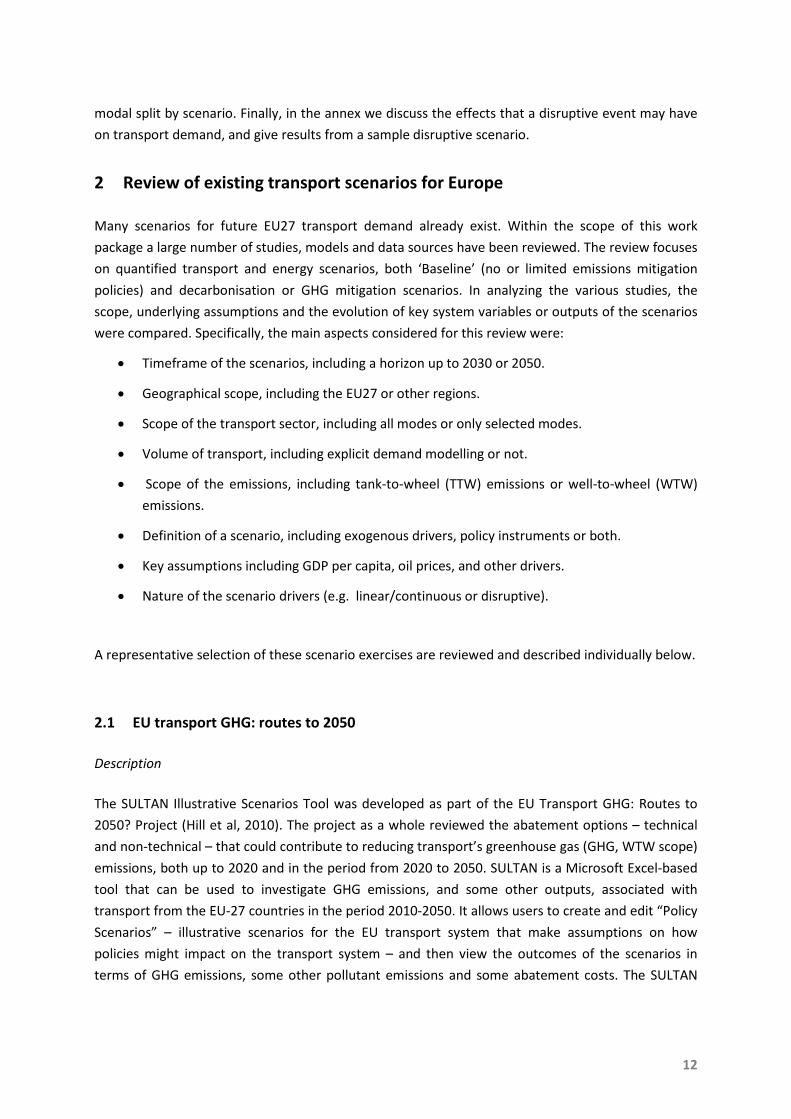
3.5 Favourable scenario
The ‘favourable’ scenario in terms of emission reductions reflects a period of economic vulnerability
in Europe. The annual GDP growth in the EU27 countries is only 0.7% throughout the whole 2010-
2050 period.
The oil price rises by 2050 up to 200 US$’08 per bbl. This may be a consequence of, for example,
limited oil supply. Due to this rise, transport costs also increase, reaching higher levels than in the
Baseline scenario. Low GDP growth and high oil prices are likely to lead to less demand for transport
and an improved business case for consumer adoption of alternative low carbon technologies and
fuels. The carbon intensity of electricity is expected to decrease by 3.0% per annum, achieving an
overall decrease of 70.4% from 2010-2050, 40% lower than the in the Baseline scenario.
The oil price demonstrates an annual growth rate of around 6.4% for the first decade, followed by a
growth rate of 1.2% from 2020 to 2040 and of 1.1% until 2050. GDP has an almost linear growth of
2.5% annually. Finally, the carbon intensity of electricity generation declines at 3% per annum5
.
These assumptions are summarised in Table 3.6.
Table 3.6 ‘Favourable’ Scenario Assumptions
Favourable Scenario 2010 2020 2030 2040 2050 Growth Rate
p.a. (2010 –
2050)
Oil Price ($’08 per bbl) 76 141 159 179 200 2.4%
Difference from Baseline 0% +38% +35% +32% +27%
GDP (billion €’09) 12492 13394 14362 15399 21999 1.4%
Difference from Baseline 0% -12% -21% -30% -15%
Carbon Intensity Electricity Generation
(gCO2/kWh)
380 280 207 152 112 -3.0%
Difference from Baseline 0% -13% -23% -33% -41%
5 The TOSCA scenarios do not consider in detail how carbon savings are made in electricity generation.
However, it should be noted that other calculations within TOSCA depend on the available biomass supply. In
these calculations it is assumed that there is not a significant use of biomass by electricity generation.

29
4 Projecting intra-European passenger and freight transport demand
In order to estimate the impact that each scenario described in Section 3 has on EU27 transport
emissions, we need to determine how transportation demand will develop in each case. Different
scenario assumptions are likely to have varying effects depending on the mode, country, population
segment and existing transportation system looked at. Therefore demand modelling that considers
these effects as far as possible is needed. This section describes the demand modelling process in
TOSCA.
4.1 European transport network model (Transtools)
As explained in chapter 1, the scenario assumptions described above are implemented within the
European transport demand model Transtools, to simulate the intra-EU demand impact for
passenger and freight transport by mode. The Transtools model input consists of a detailed database,
based on the European Transport Policy Information System (ETIS) database of transport policy-
relevant European variables, as appropriate for a 2005 base year (NEA, 2005). TOSCA input consists
of changes to the Transtools input database to reflect the development of baseline scenario variables
from 2005 for each year run (e.g. in terms of population, urbanisation, fuel prices, carbon prices) and
any development in the characteristics of the reference technologies identified by WP 1-5 (e.g. in
terms of cost, speed and fuel consumption). In the case that the database contains a cost to end-
users rather than operators (for example, rail ticket prices rather than costs accruing to rail
operators) it is assumed that all cost increases are passed on to consumers. A description of the
model itself is given below.
Transtools Demand Model
Transtools (DTU, 2010) is a large and complex demand model which includes several different,
interacting modules to calculate the end-results of passenger and freight demand, as shown in figure
4.1. These are:
• The regional economic model, which models interdependencies in economic processes
(using a multiregional computable general equilibrium model), incorporating transport costs
and other cost components.
• The freight models (mode and logistics). This module uses a top-down approach
incorporating global economic trends and national GDP, and calculates the trade volume
between countries and regions (NUTS 26
6 The EU Nomenclature of Territorial Units for Statistics (NUTS) system splits Europe into a number of
geographical regions for modelling purposes. Transtools uses NUTS2 and NUTS3-level data. These
classifications divide the EU27 countries into 271 and 1303 regions respectively.
level). The logistics module ranks the regions

30
according to their attractiveness for freight transhipment and assigns the freight demand to
the logistics chains. The output consists of trip matrices at a NUTS2 geographic level.
• The passenger demand model. This module is implemented as stored procedures in a
database. The inputs to the model are cost matrices, rail ticket prices, and zone data (e.g.
population, GDP, employment). It is specified for four trip purposes (e.g. business) for both
short and long trips (short trips do not include the air mode). The output consists of NUTS3-
level Matrices7
• The network model (for all modes). The network uses stochastic processes and calculates the
demand for each mode of transport. The road network consists of 50,000 links and 30,000
nodes, the air network 450 airports, the rail freight network from 6,000 links and 4,500
nodes and the rail passenger network 5,500 links and 4,500 nodes. The network model is
used to calculate routing and congestion on major routes, which in turn may impact demand.
.
• The air journey model. This is a stochastic model which uses the link times and the costs to
calculate the air passenger demand.
• The impact models. These are the environmental and the transport impact models. The first
includes indicators for energy consumption, emissions and external costs for road, rail and
air. The second includes the safety impact and the fatalities for road and rail.
Because network effects may impact on demand, an iterative run structure is used. Initially, the
network model is run, based on the model input variables and a starting set of demand inputs. After
this, the full passenger and freight demand models are run. Finally, the network model is run again
with the updated demand values. These steps can be iterated as necessary.
Transtools covers the whole of the EU27 and a number of other countries (e.g. the Ukraine). For the
present study, only EU27 results were extracted.
Transtools Limitations
Transtools simulates all major European networks (air, road, train and inland waterways) at NUTS2
(271 provinces/regions) and NUTS3 (1,303 districts/ groups of municipalities) geographical levels. The
output, in terms of network passenger and freight flow for a scenario year, is represented at a NUTS2
level for freight and at NUTS3 for passengers. Output is provided in vehicles-km for road transport,
tonnes-km for inland navigation and rail freight transport and passenger-km for aviation and rail
passenger transport. As well as demand flows, Transtools calculates detailed matrices for travel
costs, speed and travel times by mode as part of its demand and modal split calculations.
7 The air mode is calculated per airports (specified regions are included).

31
Figure 4.1 Transtools modules
However, Transtools has a number of limitations that means it is primarily suitable only for baseline
demand modelling within TOSCA. TOSCA has two broad requirements for demand modelling (Figure
1.6). The first is for scenario-dependent projections of demand by mode to 2050 in the case without
significant changes to vehicle technology. The second is for projections of how that demand may
change in response to developments in technology characteristics or changes in policy. Whilst the
first requirement may be satisfied with a small set or model runs per scenario, the latter case
requires a far greater number of model runs. Transtools allows a comprehensive, network-based
investigation of future transportation scenarios which includes many important effects, including
congestion and population heterogeneity. Some elements within the model are stochastic and
require several iterations for the results to stabilise. However, these factors result in a high
calculation time (approximately a week per run, where one run generates demand output for a single
year). This makes it infeasible in terms of time to run large grids of Transtools runs.
In addition, Transtools has a limited scope of the European network (e.g. covering mostly highways,
national roads, and interregional/provincial roads for the road network, and not covering tram,
metro and regional lines for railways). Whilst the network modelling carried out in Transtools is
valuable for projecting congestion effects, it is only carried out for this network scope, and modelling
outside this network is more limited. It does not model intercontinental air or marine transport, or

32
air freight. The rail modelling is limited, resulting in rough estimates of travel time, cost and flows.
Vehicle stock is also not modelled in detail.
Because of these limitations, some elements of the TOSCA demand modelling are calculated outside
the main model using alternative models. First, some demand calculations were made to cover areas
not included in Transtools. This includes estimates of intercontinental marine and air freight demand,
for which simple models from the literature were used. Intercontinental passenger aviation was
modelled using the Aviation Integrated Model (Reynolds et al. 2007). These models are described in
Section 4.2 below. In each case care was taken to ensure that the input assumptions were consistent
with those used in the Transtools input. Second, Transtools output is calculated until 2030. As not all
of the components of Transtools are designed to function after 2030, the long-term effects (beyond
2030) of the scenarios are simulated by meta-models and trend extrapolations. Besides the regular
runs for each scenario in Transtools (2010, 2020, 2030), two additional runs were used for the
Disruptive scenario (2021 and 2025) so as to fully depict the disruptive effect.
As Transtools is a network model, some of its network calculations exclude passengers and freight
travelling on minor roads or rail routes. For example, for rail transport, Transtools covers only the
main stations, excluding regional rail transport, metros and trams. This leads to underestimates
which need to be corrected for when using these calculations to estimate aggregate demand, as
discussed in TENconnect (2010). Therefore it was also necessary to calibrate the remaining data,
both rail and road transport, to Eurostat data for the base year (Eurostat, 2010) to account for these
excluded trips (see Table 4.1).
Table 4.1 Comparison of Transtools to Eurostat results
Mode Eurostat Transtools
output Divergence Rail Freight 443 461 4%
Rail Passenger 409 292 -29%
Passenger Cars 4725 4073 -14%
Trucks 1878 1897 1%
Finally, the long runtime of Transtools made it necessary to make runs before the final versions of
the results of TOSCA work packages 1-5 were available. In a few cases, the change from intermediate
to final values resulted in changes to technology characteristics which had been used as input to
Transtools. To account for these changes, the elasticity model developed as part of the stock
modelling (See WP6.2 Report, section 2.7) was used to adjust the total demand. For the scenarios
discussed here, changes were typically under 1%.

33
4.2 Intra- and intercontinental air transport and maritime transport
Passenger aviation
Transtools does not include a model for intercontinental aviation. However, there are several
reasons why having an estimate of intercontinental aviation demand is useful for the TOSCA project.
First, many intercontinental air passengers make multi-segment journeys which include an intra-EU
segment. Projections of intercontinental aviation demand typically show faster growth than for intra-
EU demand (e.g. Boeing 2010, Airbus 2009), so intra-EU journeys by intercontinental passengers will
also grow in importance in the future. Second, intercontinental and intra-EU flights share the same
airports and airspace. This means that any consideration of airport or airspace capacity is incomplete
if only one type of flight is considered. Third, although TOSCA does not consider specific alternative
technologies for long-haul aircraft, this is due to an anticipated lack of new technologies for these
aircraft which could make a significant fleet impact before 2050, not because they are unimportant
in terms of emissions. In fact, long-haul aviation is one of the fastest-growing sectors both in terms of
demand and emissions, with growth in pkm in excess of 5% per year predicted on some route groups
(Airbus 2009, Boeing 2010) and it is already included in EU climate policy via the EU’s inclusion of
aviation from 2012 in its emissions trading scheme (EU 2009). Therefore estimating intercontinental
aviation emissions is important in terms of estimating the relative importance of different future
transport emissions sources.
As Transtools excludes intercontinental transport, estimates of intercontinental aviation demand are
made using an existing model at the University of Cambridge, the Aviation Integrated Model. Since
this is a global model of aviation, it also provides an alternative forecast for intra-EU aviation. This
model, and its use within TOSCA, are described below.
Aviation Integrated Model
The Aviation Integrated Model (AIM) is a systems model of global aviation, covering around 95% of
global air pkm (Dray et al. 2010a). The future demand estimates provided by AIM are scenario-based
and require GDP, population, fuel and carbon prices as input. Output in terms of demand and
emissions is provided on a city-pair basis, allowing the change in demand over arbitrary geographical
regions to be calculated. These factors make the model suitable as a method of estimating
intercontinental aviation demand to and from the EU27 countries within TOSCA. A summary of the
model structure, inputs and outputs and use in TOSCA is given below.
Figure 4.2 shows the basic structure of AIM. AIM consists of seven interconnected modules,
programmed in Java and Matlab. Of these, only the first four are relevant for TOSCA demand
estimation.
The Air Transport Demand module projects true origin-ultimate destination demand for air travel
for a set of 700 global cities, served by 1,127 airports, which accounts for around 95% of global

34
scheduled air pkm. For use in TOSCA, population and GDP per capita from the TOSCA scenarios by
world region are provided as inputs8
.
Figure 4.2 Aviation Integrated Model structure
The Airport Activity Module assigns passenger routing, a flight schedule, and aircraft types by
flight segment, calculates the resulting flight delay and airport capacity requirements to maintain
future flight delays close to existing levels. This approach assumes that airport regions will be able to
expand runway capacity to meet demand requirements (if necessary by utilising secondary airports).
The Aircraft Movement Module calculates the location of emissions, accounting for en-route
inefficiencies.
The Aircraft Technology and Cost Module computes costs and emissions by aircraft type, and fleet
turnover rates, including airline decisions to invest in new technology. For the purposes of the TOSCA
baseline runs, it was assumed that no new technologies were available to airlines other than air
traffic management improvements provided by the SESAR project, and evolutionary replacement
narrowbody aircraft. The changes in costs resulting from these technologies were taken from TOSCA
WP2 data (Vera-Morales et al. 2011), in combination with TOSCA scenario data about fuel and
carbon prices. Airline costs are used in AIM to estimate average airfares, which are input to the Air
Transport Demand module, for the estimation of passenger demand. These modules are therefore
run iteratively until equilibrium between demand and supply is reached. For the purposes of TOSCA,
8 As noted in section 3.2, GDP scenarios for regions outside the EU27 countries are taken from Duval & de la
Maisonneuve (2009). Where population for regions outside the EU is needed, it is taken from the UN’s medium
population projection for all scenarios (UN 2009).

35
this represents the final output. More details about AIM, its previous use in modelling EU and global
policy scenarios, and the details of the individual modules may be found in Reynolds et al. (2007) and
Dray et al. (2010a, 2010b).
Multiple options are available in terms of scope when considering intercontinental pkm and tkm. For
the purposes of TOSCA, we report totals which are 50% of total intercontinental demand to and from
Europe. This effectively assigns responsibility for emissions to the country of origin for any given trip,
and allows a direct comparison of fuel use with bunker fuel totals.
Consistency
The use of different models for different modes raises potential consistency issues. In particular, two
different projections of intra-EU air demand were generated as part of the simulation process, one
by AIM and one by Transtools. Because intercontinental air passengers often include an intra-EU
flight as part of their journey (for example, flying from New York to London, then from London to
Rome), it is desirable to have projections for intercontinental and intra-EU passenger demand which
are linked, as is the case in AIM. Because intra-EU air passengers have the option of driving or taking
the train instead, it is also desirable to have projections of intra-EU demand by mode which are
linked, as is the case in Transtools.
In choosing which intra-EU projection to use within TOSCA, a comparison was made with industry
projections for future aviation demand (e.g. Boeing 2010; Airbus 2009; ICAO 2007). These
projections suggest a growth rate of 2-4% per year in intra-EU aviation pkm over the next 20 years is
anticipated by the aviation industry. AIM projections (1.6-4.5% per year) most closely matched these
growth rates, so they were used in TOSCA.
Air Cargo
Air cargo transportation is strongly linked to air passenger transportation. Around 58% of air cargo is
carried in the holds of passenger aircraft (ICAO 2008). The remaining cargo is carried in dedicated
freighter aircraft. Worldwide, these account for less than 10% of the global aircraft fleet (Morrell &
Dray 2009). Whilst dedicated freighter aircraft can be bought new, many are aircraft which were
retired from the passenger fleet and then converted to freighter usage. This results in a freighter
fleet which is typically older than the passenger fleet and has higher per-plane emissions.
Modelling air cargo demand on a network basis is a complex task, as data on current air cargo
movements is relatively sparse and can include goods which were actually shipped by truck (e.g.
Boeing 2004). The future locations of production facilities for goods which are commonly shipped by
air, and of transhipment points, can be difficult to predict. In addition, because air cargo typically
transports small amounts of low-weight, high-value goods, total tkm is almost negligible compared to
other modes (e.g. Eurostat 2010). For these reasons, air cargo is usually excluded from transportation
models. Neither AIM nor Transtools explicitly model air cargo demand or emissions. However, freight

36
carried in the holds of passenger aircraft is implicitly included via its effect on individual aircraft
weight.
To estimate the additional impact of dedicated cargo aircraft on emissions, a very simple elasticity-
based model is used here to generate demand projections. Intra-EU27 total air freight demand in
2007 was 3.1 billion tkm (Eurostat, 2010). This value is assumed to also be representative for 2009,
given the recessionary conditions in between. The corresponding base year intercontinental demand
was then estimated from a comparison of intra-EU and intercontinental freight from airline schedule
data (OAG 2005). The proportion of this freight carried in cargo aircraft was assumed to remain
constant at present-day values over the time period to 2050 (ICAO, 2008). As for air passenger
demand above, these values were then halved to obtain an estimate corresponding to bunker fuel
usage.
Secondly, GDP and price elasticities as appropriate for all-cargo carriers from Oum et al (1990) are
applied to this total to generate an idea of the total change to 2050 under different scenarios. It is
assumed that the proportion of freight carried in the holds of passenger aircraft will remain roughly
constant to 2050. These assumptions result in projected growth rates of intra-EU air cargo of 1-3%
per year, and intercontinental air cargo of around 4-5% per year. These values are low compared to
industry forecasts (e.g. Boeing 2007 predict 6%/year for global air freight tkm growth) but give a
reasonable idea of the general trend expected.
Maritime Cargo
Cargo shipping between the EU27 countries may be divided into three broad categories depending
on the geographical scope: inland waterways, short sea shipping and intercontinental shipping. In
addition, some passenger transportation is carried out by ship. Of these, by far the largest share of
emissions comes from intercontinental shipping. For example, in 2006 total EU27 shipping CO2
emissions were estimated at 195 million tonnes, of which 171 million tonnes were from
intercontinental freight transport (EC 2010). Therefore the focus of the maritime modelling in TOSCA
is on intercontinental freight shipping. This sector is not covered by Transtools so, as with aviation, a
simple alternative model based on TOSCA scenario inputs was utilised.
There exist relatively few projections of regional shipping demand on a tonne-kilometre basis. Total
seaborne trade has historically been very strongly dependent on GDP (Eyring et al., 2005a). Eyring et
al. (2005b) develop simple models for total seaborne trade in million tons and the number of ships
required as a function of GDP. In combination with TOSCA data on the typical utilisation by ship,
these models enable estimates of the growth in seaborne tkm by scenario. It should be noted,
however, that as TOSCA does not include trends in ship size over time, that the demand growth rates
here are probably underestimates. Baseline demand is estimated from bunker fuel totals, assuming
the reference ship technologies specified in TOSCA are representative of the shipping fleet. As we
exclude small ships, this also means that baseline tkm estimates will typically be higher than actual
values, since fuel use per tkm is higher for smaller ships. However, despite these simplifications,

37
these estimates result in similar growth rates in TOSCA for the numbers of ships required and CO2
emissions as in the set of projections used in Eyring et al. (2005b).
The Eyring et al (2005b) model does not include fuel price as an input variable. Fuel costs are a high
and increasing component of shipping costs (e.g. Buxton 1985). However, estimates of both the
elasticity of maritime freight rates to oil prices and the elasticity of demand for ship tkm to freight
rates are typically low. UNCTAD (2010) estimate that the elasticity of container freight rates to oil
price is between 0.19 and 0.36, whilst the corresponding value for crude oil is around 0.28. Oum et
al. (1990) give estimates of demand elasticities to freight rates for ocean shipping which range from
0.06-0.31 for commodities other than General Cargo, and 0.00-1.10 for General Cargo. In
combination, these figures suggest that GDP is a much stronger influencing factor on total maritime
shipping demand than fuel price. However, there is some evidence that the influence of oil price on
freight rates may be larger at times when the oil price is volatile (UNCTAD 2010). This may affect the
Disruptive scenario (Annex A) in particular, in which the oil price development follows that in the
baseline scenario apart from a strong peak and decline in the period 2021-2030. To account for the
effect of volatile oil price on demand in the Disruptive scenario, we calculate the relative change in
fuel prices from the Baseline scenario and apply elasticities from Hummels, Lugosky & Skiba (2007).
4.3 Aggregated Scenario Results
The following graphs depict the trends of the passenger and freight transport in passenger km and
tonne km respectively, expressed in billions. Road and Rail results come from Transtools calculations.
As discussed above, aviation demand is calculated by the AIM model and an approximate calculation
for maritime demand is made using literature values. The results do not include inland navigation
demand. This section presents the results for the three main scenarios described in Section 2:
Baseline, Favourable and Challenging. The Disruptive results will be presented in Annex A.
Growth rates by scenario and mode of transport
Demand growth rates by major intra-EU27 mode and time period are shown in Figures 4.3 – 4.5.
According to our findings, the highest growth rates in demand (excluding intercontinental transport
and air freight) occur in air passenger transport (intra-EU27). Air transport accounts for a 10% share
of passenger-km in 2010 and this increases to 26% by 2050 (Challenging scenario). At the same time,
there is a small decline in rail passenger mode share (1-2% depending on the scenario) and some
shift from road to air travel.
Another observation is that the Challenging scenario presents the highest growth rates. This is
expected as oil and electricity prices are low, and GDP growth is high. The Baseline scenario
demonstrates in general low growth in demand, which does not surpass 1.5% annually (with the
exception of aviation). In most cases the largest growth is observed in the 2020-2030 period. The
Favourable scenario is the only scenario demonstrating negative growth, primarily for rail freight
transport. It also has a high divergence between decades (for freight transport and passenger
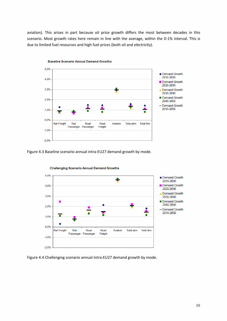
38
aviation). This arises in part because oil price growth differs the most between decades in this
scenario. Most growth rates here remain in line with the average, within the 0-1% interval. This is
due to limited fuel resources and high fuel prices (both oil and electricity).
Figure 4.3 Baseline scenario annual intra-EU27 demand growth by mode.
Figure 4.4 Challenging scenario annual intra-EU27 demand growth by mode.

39
Figure 4.5 Favourable scenario annual intra-EU27 demand growth by mode.
Growth in demand is in general consistent with that expected from the scenario definition, with the
Challenging scenario experiencing high growth and the Favourable scenario only limited growth.
Passenger km for all scenarios
0
2000
4000
6000
8000
10000
12000
14000
1995 2000 2005 2010 2015 2020 2025 2030 2035 2040 2045 2050
Billi
on p
asse
nger
-km
EC Pocketbook 2010 Scenario 0: BaselineScenario 1: Challenging Scenario 2: Favourable
Figure 4.6 Model results (intra-EU27): Total passenger-km

40
Total passenger and freight transport by scenario
Figure 4.6 depicts the total intra-European projected passenger demand for each scenario. The
overall trend is influenced mainly by the road transport demand, which also maintains the highest
share in the modal split. According to these models, by 2050, the Challenging scenario displays a
relative (to baseline) growth of almost 33%, with the total passenger-km reaching almost 13,000
billion. On the other hand, the Favourable scenario displays a relative (to baseline) decrease of
25.5%, slightly exceeding 7,000 billion passenger-km. Compared to 2010, the Favourable scenario still
shows an increase in demand to 2050 by 28%, while for the Challenging scenario that increase rises
to 128%. By maintaining the existing conditions (baseline scenario) the increase in passenger demand
will be around 72%.
Figure 4.7 shows the corresponding results for freight. Here freight displays lower growth than that
of passenger demand, but growth rates are still significant. Here the discrepancy between the
baseline and the challenging scenarios for 2050 is smaller (16%), while for the favourable scenario it
is greater (-29%). The difference between 2010 and 2050 values is as follows: the baseline results
depict a 51% increase, the challenging, a 76% increase and the favourable, a modest 8% increase.
Tonne km for all scenarios
0
500
1000
1500
2000
2500
3000
3500
4000
4500
1995 2000 2005 2010 2015 2020 2025 2030 2035 2040 2045 2050
Billi
on to
nne-
km
EC Pocketbook 2010 Scenario 0: BaselineScenario 1: Challenging Scenario 2: Favourable
Figure 4.7 Model results (intra-EU27): Total tonne-km
The effect of scenario on passenger demand seems to be significantly higher than that on freight.
This is mainly due to the presence of air passenger transport, which is sensitive to GDP changes, in

41
the above figures. Comparing only the road and rail transport modes, the differences shrink
significantly.
Passenger
Split:
Freight
Split:
Figure 4.8 Modal splits for the baseline scenario (intra-EU27)
4.4 Detailed scenario results
Baseline scenario results
This section describes the results by scenario, starting with the baseline. The output under
examination is the transport demand and how this is distributed between the different modes of
transportation. The modal split is examined for road and rail (for both freight and passengers), and
for aviation (only for passengers). In addition, the results for intercontinental aviation, air freight, and
maritime transport, are included separately. It should be noted that these latter results are
approximate only and represent the results of much less detailed models than for the other modes.
For the baseline scenario, the passenger modal split demonstrates the largest changes. This is
demonstrated in Figure 4.8. Road transport undergoes a decline of 7% in modal share which is all
absorbed by aviation (with an additional 1% in modal share from rail transport). Given that the total
passenger km in 2050 is almost 10,000 billion pkm, the shift to aviation corresponds to about 800
billion pkm. The shift to aviation can be explained through socio-economical trends such as the
increase in demand for high-speed transport with increasing GDP per capita (Schäfer & Victor, 2000).
Together, rail and air transport account for almost one fourth of the total demand. In comparison to
the passenger sector, the freight transport modal split remains almost unchanged, with an
insignificant increase of 1% for road transport, which reaches almost 3,000 billion tonne km in 2050.

42
As mentioned before, the highest demand growth rate for the baseline scenario comes from air
passenger transport (almost 3% p.a.). The other modes have a modest growth of around 1%. More
specifically, for road transport pkm increases by 1.1% p.a. and rail pkm by 0.8% p.a., while in freight
transport road tkm demand increases by 1.1% p.a. and rail tkm demand by 0.9% p.a.. Due to the high
total proportion of road transport, total passenger demand increases by 1.4% p.a. and the freight
demand by 1.0% p.a. Table 4.2 below provides the results for the baseline scenario by mode and
their average annual growth rates.
Table 4.2 Baseline scenario results (intra-EU27)
Baseline Scenario 2010 2020 2030 2040 2050 Growth 2010-2050
Rail Freight (btkm) 443 503 540 584 633 0.9%
Rail Passenger (bpkm) 409 439 469 513 561 0.8%
Passenger Cars (bpkm) 4725 5477 6198 6779 7414 1.1%
Trucks (btkm) 1878 2172 2454 2657 2878 1. %
Aviation intra-EU27 (bpkm) 558 742 1003 1322 1791 3.0%
PKM (bpkm) 5692 6658 7670 8614 9766 1.4%
TKM (btkm) 2321 2675 2994 3241 3511 1.0%
Complementary demand
Aviation intercontinental (bpkm) 801 1307 2327 3673 6018 5.2%
Air freight intra-EU27 (btkm) 1 2 2 3 3 2.2%
Air freight intercontinental (btkm) 18 28 44 63 92 4.1%
Maritime (btkm) 24258 26479 29959 33894 39505 1.2%
As well as the Transtools results, we present the calibrated AIM model results for airfreight and the
Eyring model results for maritime. Intercontinental passenger demand increases with slightly more
than 5% annual growth. As noted above, this is consistent with industry forecasts. The airfreight
demand for freight carried by all-cargo aircraft increases for both intra and outside of EU27 by 2.2%
and 4.1% respectively. This is a slightly lower rate than predicted by industry forecasts, but still
captures the expected strong growth trend. Finally, the maritime results have a small positive growth
rate of 1.2%. As noted above, this is likely an underestimate as it does not take into account
increasing ship size; however, emissions projections are still plausible.

43
Challenging scenario results
The challenging scenario simulates the behaviour of a financially booming system, where overall
transport demand is constantly growing, driven by strong GDP growth and low fuel prices. The
development of modal split is shown in Figure 4.9. The challenging scenario follows the same basic
trends as the baseline freight demand but differs with regards to the passenger split in two ways:
first, the rail demand share decreases by 3% by 2050; secondly, the aviation share penetrates the
transport demand more than in the baseline, reaching 26% by 2050. Road transport is still the
leading mode but other modes now account for more than one fourth of the total.
Passenger
Split:
Freight
Split:
Figure 4.9 Modal splits for the challenging scenario (intra-EU27)
As already mentioned, total passenger transport demand is considerably greater than in the Baseline
scenario (by almost 33%). This is a result of the growth in road and aviation. In terms of passenger
km, by 2050, the pkm difference with the baseline is 1638 bpkm for road and 1559 bpkm for
aviation; the two modes contribute equally to the total demand. These developments are consistent
with the scenario assumptions about oil price and GDP. In contrast to road and aviation, rail demand
increases with a slower rate; by 2050 the passenger rail demand share is smaller than the in the
baseline scenario. This may result in part from the constant oil price at 76$/bbl (remaining until 2050
at Baseline levels), which means that the low energy costs currently enjoyed by rail are less of an
advantage.
The same conclusion arises from the freight demand results as well. This time the modal split
remains almost constant, decreasing only in 2050 by one percentage unit. Nevertheless the annual
growth in road is greater than the rail. Overall, the passenger demand is more sensitive to the

44
Challenging conditions than the freight demand. By 2050, the difference between Challenging and
Baseline reaches 32.7% for passenger and 17.5% (almost half) for freight
Table 4.3 Comparison of Challenging to Baseline Scenario (intra-EU27)
Scenario 1: Challenging
Scenario Output Comparison to Baseline (%)
p.a.
Growth
2010 2020 2030 2040 2050 2020 2030 2040 2050
2010-
2050
Rail Freight (btkm) 443 457 583 657 732 -9.1% 8.0% 12.5% 15.6% 1.3%
Rail Passenger (bpkm) 409 442 487 523 558 0.7% 3.8% 1.9% -0.5% 0.8%
Passenger Cars (bpkm) 4725 5703 6885 7953 9052 4.1% 11.1% 17.3% 22.1% 1.6%
Trucks (btkm) 1878 2321 2662 3024 3393 6.9% 8.5% 13.8% 17.9% 1.5%
Aviation intra-EU27 (bpkm) 558 867 1370 2117 3350 16.8% 36.6% 60.1% 87.0% 4.6%
PKM (bpkm) 5692 7012 8742 10593 12960 5.3% 14.0% 23.0% 32.7% 2.1%
TKM (btkm) 2321 2778 3245 3681 4125 3.9% 8.4% 13.6% 17.5% 1.5%
Complementary demand
Aviation intercontinental (bpkm) 814 1517 3230 5907 11191 20.2% 38.8% 60.8% 86.0% 6.8%
Air freight intra-EU27 (btkm) 1 2 2 3 4 3.5% 13.2% 23.8% 35.5% 3.0%
Air freight intercontinental (btkm) 18 30 51 78 121 7.4% 15.2% 23.2% 31.2% 4.8%
Maritime (btkm) 24258 26986 31462 36947 45065 1.9% 5.0% 9.0% 14.1% 1.6%
Intercontinental aviation demonstrates the highest average growth rate (6.8% p.a.), followed by air
freight demand (intra-EU27 3.0% p.a. and intercontinental 4.8% p.a.) and, finally, maritime demand
(1.6% p.a.). These rates remain the highest within the other scenarios. Compared to the baseline, the
main discrepancy is in the intercontinental passenger aviation with a difference of 86%. This
primarily reflects the relatively high sensitivity of aviation demand to GDP growth assumed within
AIM.
Favourable scenario results
The favourable scenario simulates the lowest growth (in terms of GDP) and the highest average oil
prices. The oil prices directly influence the transport costs, which are in this case the highest for all
scenarios and all modes of transport. Therefore it is expected that the total demand is lower than the
baseline case.
Figure 4.10 below shows modal split for the years 2010, 2030 and 2050. For passenger demand one
can observe the obvious dominance of the road mode, maintaining almost 80% mode share in 2050.

45
Here, rail transport behaves similarly to the baseline scenario, maintaining 6% of the total demand in
2050. The shift to aviation is smaller here than in other scenarios (3% less than the baseline in the
year 2050) in line with the cost and GDP assumptions. As in the challenging scenario, there are
limited changes in the modal split. The favourable scenario is affected more in terms of passenger
split and in the total of the demand values (both passenger and freight).
Passenger
Split:
Freight
Split:
Figure 4.10 Modal splits for the favourable scenario (intra-EU27)
Table 4.4 clearly depicts the differences in the demand volumes compared to the baseline. In all
cases the comparison to the baseline is negative. As mentioned in figure 4.3, for the passenger
demand, besides aviation, the growth rates do not fluctuate considerably around the annual average.
In the case of aviation, the growth increases from 0.5%p.a. to 2%p.a. (for the decades of 2010-2020
and 2020-2030) and then fluctuates around this rate. This is likely a response to a couple of aviation-
specific trend discontinuities: the introduction of the replacement aircraft technology in 2025,
reducing fuel costs, and the addition of aviation to the EU emissions trading scheme in 2012. Aviation
demand demonstrates the highest growth. For the other passenger modes growth does not exceed
1% (annually).
In the favourable scenario, the rail freight has a negative growth for the first decade. Nonetheless the
total demand for freight tonne-km has a slightly increasing trend due to the higher growth of road
freight transport. In year 2030, the situation is reversed with the rail freight having a negative
growth, inducing also the decrease in total demand. After 2030 the freight demand follows a positive
growth. In total, by 2050, the total tonne-km is increased by 7.6%.
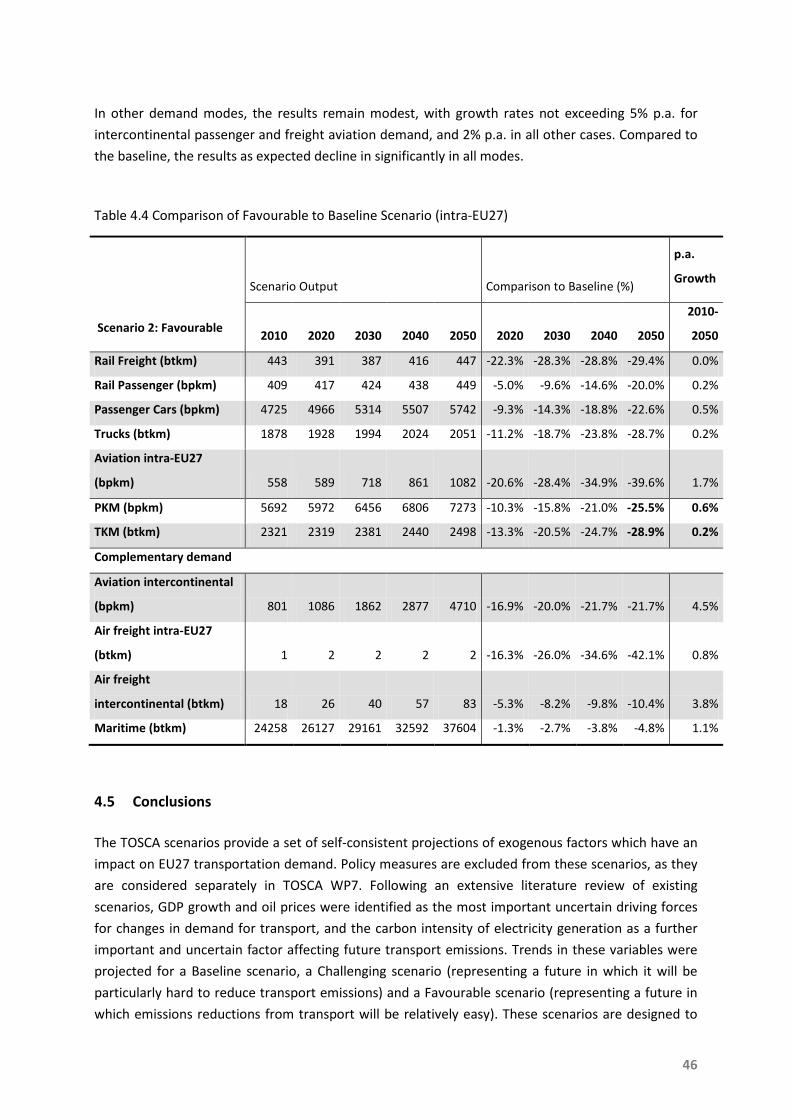
46
In other demand modes, the results remain modest, with growth rates not exceeding 5% p.a. for
intercontinental passenger and freight aviation demand, and 2% p.a. in all other cases. Compared to
the baseline, the results as expected decline in significantly in all modes.
Table 4.4 Comparison of Favourable to Baseline Scenario (intra-EU27)
Scenario 2: Favourable
Scenario Output Comparison to Baseline (%)
p.a.
Growth
2010 2020 2030 2040 2050 2020 2030 2040 2050
2010-
2050
Rail Freight (btkm) 443 391 387 416 447 -22.3% -28.3% -28.8% -29.4% 0.0%
Rail Passenger (bpkm) 409 417 424 438 449 -5.0% -9.6% -14.6% -20.0% 0.2%
Passenger Cars (bpkm) 4725 4966 5314 5507 5742 -9.3% -14.3% -18.8% -22.6% 0.5%
Trucks (btkm) 1878 1928 1994 2024 2051 -11.2% -18.7% -23.8% -28.7% 0.2%
Aviation intra-EU27
(bpkm) 558 589 718 861 1082 -20.6% -28.4% -34.9% -39.6% 1.7%
PKM (bpkm) 5692 5972 6456 6806 7273 -10.3% -15.8% -21.0% -25.5% 0.6%
TKM (btkm) 2321 2319 2381 2440 2498 -13.3% -20.5% -24.7% -28.9% 0.2%
Complementary demand
Aviation intercontinental
(bpkm) 801 1086 1862 2877 4710 -16.9% -20.0% -21.7% -21.7% 4.5%
Air freight intra-EU27
(btkm) 1 2 2 2 2 -16.3% -26.0% -34.6% -42.1% 0.8%
Air freight
intercontinental (btkm) 18 26 40 57 83 -5.3% -8.2% -9.8% -10.4% 3.8%
Maritime (btkm) 24258 26127 29161 32592 37604 -1.3% -2.7% -3.8% -4.8% 1.1%
4.5 Conclusions
The TOSCA scenarios provide a set of self-consistent projections of exogenous factors which have an
impact on EU27 transportation demand. Policy measures are excluded from these scenarios, as they
are considered separately in TOSCA WP7. Following an extensive literature review of existing
scenarios, GDP growth and oil prices were identified as the most important uncertain driving forces
for changes in demand for transport, and the carbon intensity of electricity generation as a further
important and uncertain factor affecting future transport emissions. Trends in these variables were
projected for a Baseline scenario, a Challenging scenario (representing a future in which it will be
particularly hard to reduce transport emissions) and a Favourable scenario (representing a future in
which emissions reductions from transport will be relatively easy). These scenarios are designed to

47
cover the full range of likely variation in future EU27 transportation emissions. They were used as
input to demand modelling using existing transport demand models such as Transtools and AIM.
Based on the output of these models we conclude that:
• Demand for transportation increases in all scenarios, even in the Favourable scenario. The
projected intra-EU27 passenger-kilometres travelled in 2050 varies between around 13000
billon (in the Challenging scenario) and around 7000 billion (in the Favourable scenario), in
comparison to a year-2010 value of 5692 billion. Similarly, freight tonne-kilometres travelled
in 2050 varies between 4000 billion and 2500 billion , in comparison to a year-2010 value of
2321 billion.
• The variation around the baseline demand (passenger and freight) in the challenging (+33%,
+18%) and favourable (-26%, -29%) scenarios seems plausible and wide enough for their
purpose as exogenous scenarios in TOSCA.
• In all scenarios the modal shares of freight demand (intra-EU27) per mode are similar (82%
for road and 18% for rail, excluding maritime and air freight demand). Changes in the input
assumptions as used in TOSCA do not have a strong effect on the output for the freight
model in Transtools.
• The modal shares of passenger demand (intra-EU27) show greater differences across
scenarios, with road transport remaining the dominant transport mode. The greatest trend
change concerns the Challenging scenario which shows a considerable stronger growth of
the modal split in aviation compared to the Baseline (26% of the total demand in 2050, while
the Baseline grows up to 18%).
Table 4.5 provides a numerical description of the last two findings.
The scenarios and demand projections generated in this report are used to estimate
technology uptake and transportation emissions in the second TOSCA WP6 Report. The
impact of changes in policy on demand emissions and technology utilised is then considered
in the final report of TOSCA WP7.
Table 4.5 Modal split in pkm (road, rail and aviation) and tkm (road and rail) by scenario in 2050
2050 Modal Split (intra-EU27) Road Rail Aviation
TKM
Baseline 82% 18% Challenging 82% 18% Favourable 82% 18%
PKM
Baseline 76% 6% 18% Challenging 70% 4% 26% Favourable 79% 6% 15%

48
References
AEO, 2009. American Energy Outlook, with Projections to 2030. Energy Information Administration
Office of Integrated Analysis and Forecasting, U.S. Department of Energy, Washington, DC.
<www.eia.doe.gov/oiaf/aeo/>
Airbus, 2009. “Global Market Forecast 2009-2028,” Toulouse: Airbus Industrie.
http://www.airbus.com/en/myairbus/global_market_forecast.html
Astra, 2000. Schade, W., Martino, A., Roda, M. Assessment of Transport Strategies, Milano, 2000.
Brock Blomberg, S., Hess, G. D., & Orphanides, A., 2004. “The macroeconomic consequences of
terrorism”. Journay of Monetary Economics, 51, 1007-1032.
Boeing, 2010. “Current Market Outlook 2010-2029”. Seattle: The Boeing Company.
http://www.boeing.com/commercial/cmo/
Boeing, 2004. “World Air Cargo Forecast 2004-2023”. Seattle: The Boeing Company, 2004.
Buxton, I. L., 1985. “Fuel costs and their relationship with capital and operating costs”. Maritime
Policy and Management, 12, 47-54.
DECC, 2010. Updated Energy and Emissions Projections. Department of Energy and Climate Change.
UK. June 2010.
Dray, L., Evans, A. & Schäfer, A., 2010a. "The Impact of Economic Emissions Mitigation Measures on
Global Aircraft Emissions", 10th ATIO Conference, Fort Worth, 13-15 September 2010,
http://www.arct.cam.ac.uk/aim/Documents/ATIO2010Dray.pdf
Dray, L. Evans, A., Reynolds, T., Schafer, A., 2010b. "Mitigation of Aviation Emissions of Carbon
Dioxide", Transportation Research Record, 2177, pp. 17-26.
DTU, 2010. Tras-Tools overview. Nielsen, O. A., Technical University of Denmark, Department of
Transport.
Duval, R., & de la Maisonneuve, C., 2010. “Long-run growth scenarios for the world economy”.
Journal of Policy Modeling 32, 64-80.
European Topic Centre (ETC) on Air and Climate Change (ACC), 2003. “Comparison of CO2 emission
factors for fuels used in Greenhouse Gas Inventories and consequences for monitoring and reporting
under the EC emissions trading scheme”, Technical paper, 2003.
Eurelectric. Power choices, Pathways to carbon-neutral electricity in Europe by 2050.
http://www.eurelectric.org/PublicDoc.asp?ID=63875
European Commission, 2011. White Paper: Roadmap to a Single European Transport Area – Towards
a competitive and resource efficient transport system. Com(2011), 144 final, Brussels.
European Commission, 2010a. EU Energy and Transport in Figures-Statistical Pocketbook 2010.
Publications Office of the European Union, Luxembourg.

49
European Commission, 2010b. EU Transport GHG: Routes to 2050? "Towards the decarbonization of
the eu‘s transport sector by 2050, Brussels.
European Commission, 2009a. “Directive 2008/101/EC of the European Parliament,” Official Journal
of the European Union, January 13, 2009, pp. 3-21.
European Commission, 2009b. Directive 2009/28/EC of the European Parliament and the Council of
23 April 2009 on the promotion of the use of energy from renewable sources and amending and
subsequently repealing Directives 2001/77/EC and 2003/30/EC, 5 June 2009, pp. 16-62.
European Commission, 2009c. EU Energy and Transport in Figures-Statistical Pocketbook 2009.
Publications Office of the European Union, Luxembourg.
European Commission, 2008a. Proposal for a Directive of the European Parliament and of the
Council on “the promotion of the use of energy from renewable sources”, 23 January 2008.
European Commission, 2008b. The EU climate and energy package,
http://ec.europa.eu/environment/climat/climate_action.htm
European Commission, 2007. Communication from the Commission to the European Parliament, the
Council, the Economic and Social Committee and the Committee of the Regions “Limiting Global
Climate Change to 2 degrees Celsius The way ahead for 2020 and beyond”, Brussels, 10 January
2007.
European Commission, 2006. Communication from the Commission “An EU Strategy for Biofuels”, 8
February 2006.
European Commission, 2005. Communication from the Commission “Biomass Action Plan”, 7
December 2005.
European Commission, 2003. “Directive 2003/30/EC of the European Parliament and of the Council
of 8 May 2003 on the promotion of the use of biofuels or other renewable fuels for transport”, 8 May
2003, pp. 42-46
European Commission, 2001. Communication from the Commission to the European Parliament, the
Council, the Economic and Social Committee and the Committee of the Regions on “alternative fuels
for road transportation and on a set of measures to promote the use of biofuels”, 7 November 2001.
E3M-Lab,GEM-E3. URL:
<http://www.e3mlab.ntua.gr/e3mlab/index.php?option=com_content&view=category&id=36%3Age
m-e3&Itemid=71&layout=default&lang=en>
E3M-Lab,PROMETHEUS. URL :
<http://www.e3mlab.ntua.gr/e3mlab/index.php?option=com_content&view=category&id=37%3Apr
ometheus&Itemid=72&layout=default&lang=en>
E3M-Lab, 2010. EU energy trends to 2030, Update 2009. Luxembourg. August 2010
Eurostat, 2010. Eurostat online database: transport statistics.
<http://epp.eurostat.ec.europa.eu/portal/page/portal/transport/data/database>.

50
Eyring, V., Köhler, H. W., van Aardanne, J. & Lauer, A., 2005a. “Emissions from international
shipping: 1. The last 50 years”. J. Geophys. Res., 110, D17305.
Eyring, V., Köhler, H. W., Lauer, A. & Lemper, B., 2005b. “Emissions from international shipping: 1.
Impact of future technologies on scenarios until 2050”. J. Geophys. Res., 110, D17306.
Glick, R., & Taylor, A. M., 2005. “Collateral Damage: Trade Disruption and the Economic Impact of
War”. Federal Reserve Bank of San Francisco Working Paper Series, 2005-11.
Hill, N., Morris, M. and Skinner, I. (2010). SULTAN: Development of an Illustrative Scenarios Tool for
Assessing Potential Impacts of Measures on EU Transport GHG. Task 9 Report VII produced as part of
contract ENV.C.3/SER/2008/0053 between European Commission Directorate-General Environment
and AEA Technology plc; <www.eutransportghg2050.eu>
Hummels, D., V. Lugovsky, and A. Skiba, 2007. “The Trade Reducing Effects of Market Power in
International Shipping”. NBER Working Paper 12914. Cambridge, MA: National Bureau of Economic
Research.
ICAO, 2008. ICAO Global Database. <http://icaodata.com>.
ICAO, 2007. “Outlook for Air Transport to the Year 2025,” ICAO Publications, Clr 313 AT.134,
September 2007.
International Energy Agency (IEA), 2009. Transport, energy and CO2, 2009, Paris.
International Energy Agency (IEA), 2008. Energy technology perspectives 2008, Paris.
International Energy Agency (IEA), 2010. Energy Balances pf OECD countries 2010, Paris.
iTREN, 2009. Integrated transport and energy baseline until 2030, Deliverables 1-4. 2009. <
http://www.tmleuven.be/project/itren2030/home.htm >
JRC, 2010. Transtools website in: <http://energy.jrc.ec.europa.eu/transtools/TT_model.html>
McKinsey & Company, 2009. Roads toward a low-carbon future: reducing CO2 emissions from
passenger vehicles in the global road transportation system.
NEA, 2005. Core Database Development for the European Transport policy Information System
(ETIS), Final Technical report to the European Commission.
Tetraplan/MCRIT, 2009. TRANSvisions: Mobility scenarios toward a post-carbon society: Transvisions
Task 2 Quantitative scenarios.
Manne, A. S., Richels, R. G., Edmonds, J. A., 2005. Market Exchange Rates or Purchasing Power
Parity: Does the Choice Make a Difference to the Climate Debate? Climatic Change, 71, 1-8.
Morrell, P., & Dray, L. M., 2009. Environmental Aspects of Fleet Turnover, Retirement and Life Cycle.
Final Report for the Omega Consortium, 2009.
OAG, 2005. OAG Global Schedule Database. <http://www.oagdata.com>.
Oum, T. H., Waters, W. G., Yong, J. S., 1990. “A Survey of Recent Estimates of Price Elasticities of
Demand for Transport”, Infrastructure and Urban Development Department, The World Bank,
Washington, DC.
51
Poles, 2006. Enerdata. Prospective Outlook on Long-term Energy Systems, A World Energy Model.
2006
PRIMES, 2010. E3M-Lab. PRIMES Model, E3Mlab of ICCS/NTUA, Version used for the 2010 Scenarios
for the European Commission including new sub-models. 2010
Reynolds, T., Barrett, S., Dray, L., Evans, A., Köhler, M., Vera-Morales, M., Schäfer, A., Wadud, Z.,
Britter, R., Hallam, H. & Hunsley, R., 2007. "Modelling Environmental & Economic Impacts of
Aviation: Introducing the Aviation Integrated Modelling Project", 7th ATIO Conference, Belfast, UK,
18-20 September 2007. <http://www.arct.cam.ac.uk/aim/Documents/ATIO2007_AIMIntro.pdf>.
Schäfer, A., & Victor, D., 2000. The future mobility of the world population. Transportation research
part A, 34(3), 171-205.
TENconnect, 2010. TRANS-TOOLS version 2; Model and Data Improvements, Final Report, DG TREN,
Brussels, 2010.
TRANSvisions, 2009a. Report on Transport Scenarios with a 20 and 40 Year Horizon, Final Report,
Tetraplan A/S, Project funded by DG TREN. March 2009
TRANSvisions, 2009b. TRANSvisions Task 2 Quantitative Scenarios, Mobility scenarios toward a post-
carbon society. MCRT. March 2009.
TREMOVE, 2007. Transport & Mobility Leuven . Service contract for the further development and
application of the transport and environmental TREMOVE model Lot 1 (Improvement of the data set
and model structure), Final Report, DG TREN, Brussels, 2007.
UN, 2009. World Population Prospects: the 2008 Revision Population Database.
http://esa.un.org/unpp/
UNCTAD, 2010. “Oil Prices and Maritime Freight Rates: An Empirical Investigation”. United Nations,
New York and Geneva.
Vera-Morales, M., Graham, W., Hall, C. & Schäfer, A., 2011. Techno-Economic Analysis of Aircraft:
TOSCA WP2 Final Report.

52
List of Figures
Figure 1.1 Final EU27 Energy Consumption by Sector ............................................................................ 8
Figure 1.2 Indexed evolution of CO2 Emissions by Sector, EU27 ............................................................ 8
Figure 1.3 Indexed evolution of CO2 emissions by transport mode, EU27 ............................................. 9
Figure 1.4 Indexed evolution of GDP, population and GHG emissions from freight and passenger
transport demand ................................................................................................................ 10
Figure 1.5 TOSCA Work Package structure ........................................................................................... 10
Figure 1.6 TOSCA Modelling approach .................................................................................................. 11
Figure 3.1 Assumptions for Oil prices in all scenarios ........................................................................... 23
Figure 3.2 Assumptions for GDP in all scenarios ................................................................................... 23
Figure 3.3 Assumptions for Carbon Intensity of electricity generation in all scenarios ........................ 24
Figure 4.1 Transtools modules .............................................................................................................. 31
Figure 4.2 Aviation Integrated Model structure ................................................................................... 34
Figure 4.3 Baseline scenario annual intra-EU27 demand growth by mode. ......................................... 38
Figure 4.4 Challenging scenario annual intra-EU27 demand growth by mode. ................................... 38
Figure 4.5 Favourable scenario annual intra-EU27 demand growth by mode. .................................... 39
Figure 4.6 Model results (intra-EU27): Total passenger-km ................................................................. 39
Figure 4.7 Model results (intra-EU27): Total tonne-km ........................................................................ 40
Figure 4.8 Modal splits for the baseline scenario (intra-EU27) ............................................................. 41
Figure 4.9 Modal splits for the challenging scenario (intra-EU27) ........................................................ 43
Figure 4.10 Modal splits for the favourable scenario (intra-EU27) ....................................................... 45
Figure 0.1 Oil prices including the Disruptive Scenario (the three stages are apparent) ..................... 54
Figure 0.2 GDP values including the Disruptive Scenario (the three stages are apparent) .................. 55
Figure 0.3 Carbon Intensity values including the Disruptive Scenario (same as the Baseline) ............. 55
Figure 0.4 Evolution of pkm in scenarios and sensitivity case .............................................................. 58
Figure 0.5 Evolution of tkm in scenarios and sensitivity case ............................................................... 59

53
Annex A: Sensitivity Analysis - Disruptive Scenario
Assumptions
Future scenarios tend to assume smooth trends in projected scenario values over time. However,
effects may arise from fluctuations in scenario values which would not be predicted in a scenario
with the same average growth rate. For example, volatility in fuel prices affects risk perception in
user and policymaker decision making. A peak in fuel prices may result in technology investment with
benefits that are observed even after the fuel price has decreased. Conversely, it may result in a
decrease in demand and an oversupply in the vehicle fleet, delaying the penetration of new vehicle
technology. In this section we define a Disruptive scenario which, studies the occurrence of an
extreme event having a disruptive and challenging impact on transport GHG emissions. This scenario
serves as a sensitivity analysis in the TOSCA scenario building framework. Extreme events may have a
catalyst effect and structurally change the transport system or economy/society as a whole. Between
2000 and 2010, the world has witnessed several extreme events having an impact specifically on the
transport sector. The SARS outbreak and the 9/11 attack in New York affected the air transport
sector in particular. However, a couple of years after 9/11 the demand for air transport had returned
to the pre-9/11 growth rates. The oil crises in the 1970s led to structural changes in many countries.
Switzerland, for example, structurally reduced its dependence on oil as a primary energy source. The
2011 nuclear crisis after the earth quake and the following Tsunami in Japan highlights how the
public opinion towards nuclear energy may change drastically. As nuclear power is a zero carbon
energy source, changing attitudes and the abandoning of nuclear programmes may lead to more
coal-fired electricity generation and resulting carbon emissions.
For the Disruptive scenario, assumptions regarding the three main uncertain and relevant scenario
variables are equal to those in the baseline scenario until 2020. After this point, the following
assumptions are made:
• Around the year 2020 an extreme event will take place, with a mixture of short-term and
continuous effects afterwards.
• The impacts of this event are similar to those of a major terrorist attack or highly infectious
disease outbreak.
• Transport modes/locations that appear most vulnerable to this continuous threat are (mass)
public transport, air transport and transport infrastructure hubs (main railway stations and
airports).
• This will result in more decentralized land use and transport planning and a modal shift of
passenger transport from (mass) public transport towards more individual modes of
transport.
• These broad impacts are specifically implemented by an oil price peak in 2021 (US$ >300),
longer waiting times and higher ticket prices for aviation and rail due to intensified security
procedures, a lower urbanisation rate than the baseline and a short-term decrease in GDP.
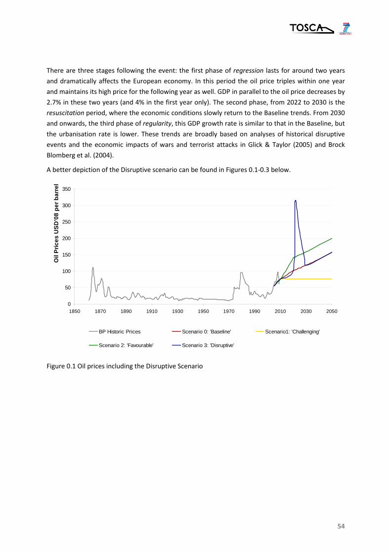
54
There are three stages following the event: the first phase of regression lasts for around two years
and dramatically affects the European economy. In this period the oil price triples within one year
and maintains its high price for the following year as well. GDP in parallel to the oil price decreases by
2.7% in these two years (and 4% in the first year only). The second phase, from 2022 to 2030 is the
resuscitation period, where the economic conditions slowly return to the Baseline trends. From 2030
and onwards, the third phase of regularity, this GDP growth rate is similar to that in the Baseline, but
the urbanisation rate is lower. These trends are broadly based on analyses of historical disruptive
events and the economic impacts of wars and terrorist attacks in Glick & Taylor (2005) and Brock
Blomberg et al. (2004).
A better depiction of the Disruptive scenario can be found in Figures 0.1-0.3 below.
0
50
100
150
200
250
300
350
1850 1870 1890 1910 1930 1950 1970 1990 2010 2030 2050
Oil
Pric
es U
SD'0
8 pe
r bar
rel
BP Historic Prices Scenario 0: 'Baseline' Scenario1: 'Challenging'
Scenario 2: 'Favourable' Scenario 3: 'Disruptive'
Figure 0.1 Oil prices including the Disruptive Scenario

55
0
5000
10000
15000
20000
25000
30000
35000
40000
1990 2000 2010 2020 2030 2040 2050
EU27
GDP
in b
illio
n EU
R'09
Eurostat Scenario 0: 'Baseline'
Scenario 1: 'Challenging' Scenario 2: 'Favourable'
Scenario 3: 'Disruptive'
Figure 0.2 GDP values including the Disruptive Scenario
0
200
400
600
800
1000
1200
1960 1970 1980 1990 2000 2010 2020 2030 2040 2050
Car
bon
Inte
nsity
g C
O 2 /
kWh
World energy balances (IEA, 2010) and Emission Factors (ETC/ACC, 2003)Scenario 0: 'Baseline' Scenario1: 'Challenging'Scenario 2: 'Favourable' Scenario 3: 'Disruptive'
Figure 0.3 Carbon Intensity values including the Disruptive Scenario (same as the Baseline)
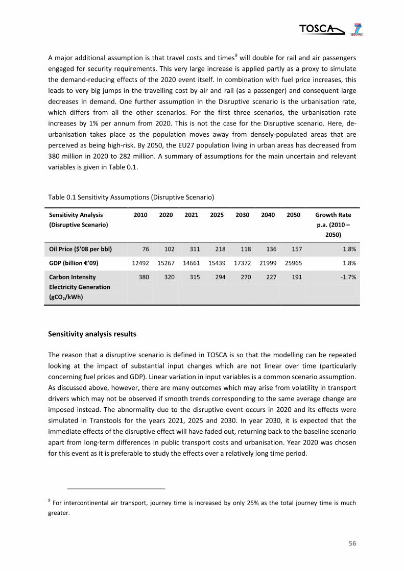
56
A major additional assumption is that travel costs and times9
will double for rail and air passengers
engaged for security requirements. This very large increase is applied partly as a proxy to simulate
the demand-reducing effects of the 2020 event itself. In combination with fuel price increases, this
leads to very big jumps in the travelling cost by air and rail (as a passenger) and consequent large
decreases in demand. One further assumption in the Disruptive scenario is the urbanisation rate,
which differs from all the other scenarios. For the first three scenarios, the urbanisation rate
increases by 1% per annum from 2020. This is not the case for the Disruptive scenario. Here, de-
urbanisation takes place as the population moves away from densely-populated areas that are
perceived as being high-risk. By 2050, the EU27 population living in urban areas has decreased from
380 million in 2020 to 282 million. A summary of assumptions for the main uncertain and relevant
variables is given in Table 0.1.
Table 0.1 Sensitivity Assumptions (Disruptive Scenario)
Sensitivity Analysis
(Disruptive Scenario)
2010 2020 2021 2025 2030 2040 2050 Growth Rate
p.a. (2010 –
2050)
Oil Price ($’08 per bbl) 76 102 311 218 118 136 157 1.8%
GDP (billion €’09) 12492 15267 14661 15439 17372 21999 25965 1.8%
Carbon Intensity
Electricity Generation
(gCO2/kWh)
380 320 315 294 270 227 191 -1.7%
Sensitivity analysis results
The reason that a disruptive scenario is defined in TOSCA is so that the modelling can be repeated
looking at the impact of substantial input changes which are not linear over time (particularly
concerning fuel prices and GDP). Linear variation in input variables is a common scenario assumption.
As discussed above, however, there are many outcomes which may arise from volatility in transport
drivers which may not be observed if smooth trends corresponding to the same average change are
imposed instead. The abnormality due to the disruptive event occurs in 2020 and its effects were
simulated in Transtools for the years 2021, 2025 and 2030. In year 2030, it is expected that the
immediate effects of the disruptive effect will have faded out, returning back to the baseline scenario
apart from long-term differences in public transport costs and urbanisation. Year 2020 was chosen
for this event as it is preferable to study the effects over a relatively long time period.
9 For intercontinental air transport, journey time is increased by only 25% as the total journey time is much
greater.

57
Table 0.2 Disruptive scenario results
Scenario 2: Favourable
Scenario Output (in pkm/ tkm & Modal split) p. a. Growth
2010 2020 2021 2025 2030 2040 2050
2010 –
2050
Rail Freight (btkm)
4725
(83%)
5477
(82%)
4596
(89%)
5101
(89%)
6829
(90%)
7768
(90%)
8809
(90%)
1.6%
0.2%
Rail Passenger (bpkm)
409
(7%)
439
(7%)
295
(6%)
290
(5%)
297
(4%)
272
(3%)
219
(2%)
-1.5%
-3.1%
Passenger Cars (bpkm)
558
(10%)
742
(11%)
248
(5%)
314
(6%)
458
(6%)
552
(6%)
719
(7%)
0.6%
-0.9%
Trucks (btkm)
443
(19%)
503
(19%)
604
(28%)
575
(25%)
538
(18%)
597
(18%)
648
(18%)
1.0%
-0.1%
Aviation intra-EU27 (bpkm)
1878
(81%)
2172
(81%)
1577
(72%)
1762
(75%)
2398
(82%)
2664
(82%)
2901
(82%)
1.1%
0.0%
PKM (bpkm) 5692 6658 5139 5705 7584 8592 9747 1.4%
TKM (btkm) 2321 2675 2181 2337 2936 3261 3549 1.1%
Complementary demand
Aviation intercontinental (bpkm) 801 1306 461 674 1210 1886 3101 3.4%
Air freight intra-EU27 (btkm) 1 2 1 1 2 2 3 2.8%
Air freight intercontinental (btkm) 18 24 11 19 44 62 91 4.1%
Maritime (btkm) 24258 26479 24662 26399 29891 33733 39222 1.2%
The results from the sensitivity analysis are shown in Table 0.2. For the years after the disruptive
effect both passenger and transport demand are significantly influenced in terms of modal split and
in total amount of pkm/ tkm. The lowest values are indicated for the year after the event (2021).
Passenger demand is slightly more affected than the freight demand. Nevertheless, both show a
positive average annual growth for the 2010-2050 time-period.
For the passenger demand, each mode behaves differently. Road demand is recuperating after 2021
and by 2030 it already exceeds the 2020 levels. This is in part due to the impact of de-urbanisation
and mode shift due to high rail and air costs. Aviation demand, on the other hand, is affected by the
assumed long-term price increases and even though it increases between 2021 and 2030, it does not
return to year-2020 levels. Finally, the rail demand demonstrates a negative slope until 2050. This is a
response to the assumed cost increases. The modal split is also affected. The rail percentage is
almost eliminated by 2050 with only 2% of the total. Aviation also decreases in mode share to 2050.
This increases the road share which reaches 90% by 2050.
Freight demand also changes radically. The road freight follows the trend of road passenger demand
and recuperates by 2030, demonstrating the highest per annum growth. This is again in part due to

58
de-urbanisation. Rail freight behaves differently. Contrary to all other modes, it increases in 2021 and
then starts dropping until 2030. By 2050, rail freight has returned to baseline growth rates. The
modal split also changes for the years 2021 and 2025, indicating a shift to rail. This is explained
through the interplay between the oil price increase and the GDP decline. The oil price in 2021 is very
high, making the price of transporting freight by road go up (more so than for rail, where a smaller
proportion of costs are fuel), so there is a shift to rail freight. GDP has also gone down, leading to a
decline in total tkm, but the shift to rail is big enough that rail sees an increase in total. By 2025, oil
prices have decreased significantly from their peak, but the GDP reduction from the baseline is
similar to that in 2021. Therefore total demand is still depressed, but there is less incentive to switch
to rail transport, so some of the 2025 demand shifts back to road. The other modes display similar
effects for the years 2021 and 2025. An overview of results is given in Figures 0.4 and 0.5.
Passenger km for all scenarios
0
2000
4000
6000
8000
10000
12000
14000
1995 2000 2005 2010 2015 2020 2025 2030 2035 2040 2045 2050
Bill
ion
pass
enge
r-km
EC Pocketbook 2010 Scenario 0: BaselineScenario 1: Challenging Scenario 2: FavourableSenisitivity Analysis (Disruptive Scenario)
Figure 0.4 Evolution of pkm in scenarios and sensitivity case

59
Tonne km for all scenarios
0
500
1000
1500
2000
2500
3000
3500
4000
4500
1995 2000 2005 2010 2015 2020 2025 2030 2035 2040 2045 2050
Billi
on to
nne-
km
Scenario 0: Baseline EC Pocketbook 2010Scenario 1: Challenging Scenario 2: FavourableSenisitivity Analysis (Disruptive Scenario)
Figure 0.5 Evolution of tkm in scenarios and sensitivity case
The effects of the disruptive event are obvious also for the other transport modes. For the years
2021 and 2025 all modes decline, especially intercontinental aviation (both passenger and freight).
Maritime transport is the least affected.
Conclusions
Based on this disruptive scenario exercise we conclude that it is generally difficult to reliably estimate
the impact of extreme events because:
• The timing of the disruptive event is arbitrary
• The number of the disruptive events is arbitrary
• Existing models are not suitable to predict extreme changes. Consumer preference dynamics
are often not covered by transport models like Transtools and TREMOVE. The underlying
elasticities in these models are often based on existing (or historical) price elasticities or
utility functions. These are only valid for moderate changes from this baseline reference
situation.
• The existing models cannot cope with memory effects after a disruptive event.
• Therefore this scenario is used only as a sensitivity test, rather than as one of the main
TOSCA scenarios.