School of Mathematical and Physical Sciences

Department of Mathematics and Statistics

Preprint MPS_2010-28

10 September 2010

Initial Distribution Spread: A density forecasting approach

by

R.L. Machete and I.M. Moroz

Initial Distribution Spread: A density forecasting approach

R. L. Machetea,1

and I. M. Morozb

a. Dept. of Mathematics and Statistics, P. O. Box 220, Reading, RG6 6AX, UK

b. Mathematical Institute, 24-29 St Giles’, Oxford, OX1 3LB

Abstract

Ensemble forecasting of nonlinear systems involves the use of a model to runforward a discrete ensemble (or set) of initial states. Data assimilation techniquestend to focus on estimating the true state of the system, even though model errorlimits the value of such efforts. This paper argues for choosing the initial ensemblein order to optimise forecasting performance rather than estimate the true state ofthe system. Density forecasting and choosing the initial ensemble are treated asone problem. Forecasting performance can be quantified by some scoring rule. Inthe case of the logarithmic scoring rule, theoretical arguments and empirical resultsare presented. It turns out that, if the underlying noise spread of the time seriesexceeds the spread of one step forecast errors, we can diagnose the underlying noisespread regardless of the noise distribution.

Keywords: data assimilation; density forecast; ensemble forecasting; uncertainty

1 Introduction

Given an initial state of some chaotic dynamical system − examples of which includethe population of an animal species in a game reserve, daily weather for Botswana orday to day electricity demands for London − we could perform a point forecast from thesingle state. Observational uncertainty and/or model error could limit the value of such aforecast. One can go over these hurdles by generating a discrete set of initial states in theneighbourhood of the current state and then forecasting from it. The set of initial statesis called an initial ensemble. Forecasting from an initial ensemble is called ensemble

forecasting [1]. The time ahead at which forecasts are made from any member of theinitial ensemble is called lead time. Ensemble forecasting is performed mainly to accountfor uncertainty in the initial conditions, although it can also be used to mitigate modelerror. A lot of attention has been paid to generating initial ensembles (e.g see [1, 2]).Here, we present a novel approach to selecting the spread of the distribution from whichan initial ensemble is drawn. The distribution from which an initial ensemble is drawnshall be called the initial distribution. Its covariance matrix will be taken to be diagonaland uniform over all the initial conditions considered, in tune with common practicein data assimilation and ensemble forecasting [1, 3, 4]. Note, however, that we do notassume that the initial distribution is the underlying noise distribution.

1Corresponding author: r.l.machete@reading.ac.uk, tel: +44(0)118 378 5016Abbreviations: Initial Distribution Spread (IDS), Perfect Model Scenario (PMS), Imperfect

Model Scenario (IMS), Moore-Spiegel (M-S), European Centre for Medium-Range Weather Fore-casts (ECMWF)

1

Ideally, the initial ensemble should be drawn from the underlying invariant measure,in which case we have a perfect initial ensemble. A perfect initial ensemble is especiallyuseful in the scenario when our forecasting model is isomorphic to the model that gen-erated the data, which scenario is called the perfect model scenario (PMS) [2, 5]. Whenthere is no isomorphism between the forecasting model and the model that generatedthe data, then we are in the imperfect model scenario (IMS). A perfect model with aperfect initial ensemble would give us a perfect forecast [6]. If either our model or initialensemble is not perfect, then we have no reason to expect perfect forecasts.

In all realistic situations, we have neither a perfect model nor a perfect initial ensem-ble, yet we may be required to issue a meaningful forecast probability density function(pdf). Roulston and Smith [7] proposed a methodology for making forecast distributionsthat are consistent with historical observations from ensembles. This is necessary be-cause the forecast ensembles are not drawn from the underlying invariant measure dueto either imperfect initial ensembles or model error. Their methodology was extendedby Broecker and Smith [8] to employ continuous density estimation techniques [9, 10]and blend the ensemble pdfs with the empirical distribution of historical data, which isreferred to as climatology. The resulting pdf is what will be taken as the forecast pdf inthis paper.

The quality of the forecast pdfs can be assessed using the logarithmic scoring ruleproposed by Good [11] and termed ignorance by Roulston and Smith [12], borrowed frominformation theory [13, 14]. Here, we discuss a way of choosing the initial distributionspread (IDS) to enhance the quality of the forecast pdfs. The point is that if the spreadis too small our forecasts may be over confident and if it is too large our forecastsmay have low information content. Our goal is to choose an IDS that yields the mostinformative forecast pdfs and determine, for instance, if this varies with the lead time ofinterest. As is commonly done in data assimilation and ensemble forecasting (e. g. see[1, 15]), we only consider Gaussian initial distributions. In traditional data assimilationand ensemble forecasting techniques, estimation of the initial distribution is divorcedfrom forecasting: this is the main point of departure in our approach. We revisit thislater in the discussion of the results in § 5.

Our numerical forecasting experiments were performed on the Moore-Spiegel (M-S) [16] system and an electronic circuit motivated by the M-S system. Indeed electroniccircuits have been studied to enhance our understanding of chaotic systems and Chuacircuits [17] are among famous examples. Recently, Gorlov and Strogonov [18] appliedARIMA models to forecast the time to failure of Integrated Circuits. Hence, electroniccircuits have not only been studied to enhance our understanding of chaotic systemsand the forecasting of real systems, but also to understand the circuits themselves andto address practical design questions.

This paper is organised as follows: § 2 introduces the technical framework for dis-cussing probabilistic forecasting of deterministic systems. The theoretical and empiricalscores for probabilistic forecasts are presented in §3. Computations of the initial ensem-ble spread are discussed in § 4 for the PMS and IMS. In the PMS, the M-S system [16]is considered. For the IMS, the M-S system and an electronic circuit are modelled usingradial basis function (rbf) models. The circuit was constructed in a physics laboratoryusing state of the art equipment to mimic the M-S system. A theoretical argument insupport of the numerical results is also presented. Implications and practical relevanceof the results are discussed in § 5 and concluding remarks are given in § 6.

2

2 Forecasting

Consider a deterministic dynamical system,

x = F (x(t),λ), (1)

with the initial condition x(0) = x0, where x,F ∈ Rm, λ ∈ R

d is a vector of parameters,F is a Lipschitz continuous (in x), nonlinear vector field and t is time. By Picard’stheorem [19], (1) will have a unique solution, say ϕt(x0;λ). If ∇.F < 0, this systemmight have an attractor [20], which if it exists we denote by A. In particular, we areinterested in the case when the flow on this attractor is chaotic.

2.1 Forecast Density

For any point in state space, x, and positive real number ǫ, let Bx(ǫ) denote an ǫ-ballcentred at x. Suppose that is some invariant measure (see appendix A) associatedwith the attractor A. For any x0 ∈ A, we define a new probability measure associatedwith Bx0

(ǫ) by

0(E) = limT→∞

1

T(Bx0(ǫ))

∫ T

01E∩Bx0

(ǫ)(x(t))dt, (2)

where 1 is an indicator function. This measure induces some probability density func-tion, p0(x,x0, ǫ). We will call a set of points drawn from p0(x;x0, ǫ) a perfect initial

ensemble. At any time t, the forecast of the perfect initial ensemble using the flow ϕt willbe distributed according to some pdf pt(x;x0, ǫ). The pdf pt(x;x0, ǫ) will be referredto as a perfect forecast density at lead time t.

2.2 Imperfect Forecasts

Operationally, we never get perfect forecasts since our initial ensemble is never drawnfrom p0(x,x0, ǫ) and our model, ϕt(x), is always some approximation of the system,ϕt(x), which possibly lives in a different state space. In that case, our forecast pdf wouldbe ft(x;x0, ǫ) rather than the perfect forecast pt(x;x0, ǫ). Henceforth we suppress theǫ dependence.

3 Scoring Probabilistic Forecasts

The next question would be: how close is ft(x;x0) to pt(x;x0)? In a general sense, weconsider the score of a forecast ft(x;xτ ) and denote it by S(ft(x;xτ ),X) [21], whereX is the random variable of which x is a particular realisation. If X is distributedaccording to pt(x;xτ ), the expected score of ft is

E[S(ft(x;xτ ),X)] =

∫

S(ft(x;xτ ),z)pt(z;xτ )dz. (3)

At lead time, t, the overall forecast score on the attractor is

E[S(t)] = limT→∞

1

T

∫ T

0E[S(ft(x;xτ ),X

(τ))]dτ, (4)

3

where X(τ) is the random variable being forecast from the initial distribution corre-sponding to xτ . Provided the underlying attractor is ergodic, we can rewrite (4) as

E[S(t)] = limT→∞

1

T

∫ T

0S(ft(x;xτ ),X

(τ))dτ. (5)

For each forecast, the underlying system can only furnish one verification of X andnot the distribution pt(x;x0). Therefore, we use (5) to score forecasts rather than (4).Discretise time according to τi = (i − 1)τs, for i = 1, 2, .., N , where τs is the samplingtime. This gives a sequence of forecast pdfs, {ft(x;xi)}N

i=1, corresponding to verifications{X(i)}N

i=1 and score S. We can thus discretise (5) to obtain the following empirical scoreto value the t-ahead forecast system:

〈S〉(t) =1

N

N∑

i=1

S(ft(x;xi),X(i)). (6)

This is the same score proposed by Broecker and Smith [21].In this paper, we shall use the score:

S(ft,X) = ign(ft,X), (7)

where ign(ft,X) = − log ft(X) is “the information deficit or Ignorance that a forecasterin possession of the pdf has before making the observation X” [12]. An importantproperty of this score is that it is strictly proper. A strictly proper score is one forwhich (3) assumes its minimum if and only if ft = pt [22]. Another property of theIgnorance score, although less persuasive, is locality. A score is local if it only requiresthe value of the forecast pdf at the verification to be evaluated [21].

4 Initial Distribution Spread

The primary concern is to determine optimal initial distribution spreads for the fore-casting problem. Each initial ensemble is drawn from a Gaussian distribution centredat the initial observation. The problem is then reduced to finding the optimal spread ofthe Gaussian distribution. An optimal spread is one that minimises the average score atthe lead time of interest. In the theoretical setup this score would be the one given byequation (4) and in an operational setup we would use the empirical score given by (6).In the numerical examples considered in this section, we use continuous forecast pdfsobtained from discrete forecasts as discussed in [8].

The cases considered are the PMS and the IMS. In the PMS, numerical experimentsare performed on the M-S system [16] at classical parameter values. In the IMS, the M-Ssystem and circuit are considered and the models are constructed from data using cubicrbf’s (see [23, 24] for details). We shall denote the spread of the underlying Gaussiandistribution of the initial ensemble by σe and that of observational noise by δ. For agiven observational noise level, we vary σe logarithmically between 10−3 and 1. δ = 0will represent the noise-free case. In the multivariate case, we set σe to be the spreadof the perturbation of the ith coordinate and then set the standard deviation of theperturbation of the jth coordinate to be

σ(j)e = σe

σj

σi, (8)

where σj is the standard deviation of the jth variable.

4

−10−5

05

10

−100

0

100

200

−2

−1.5

−1

−0.5

0

0.5

1

1.5

xy

z

Figure 1: The graph of the M-S attractor at parameter values T = 36 and R = 100.

4.1 Perfect Model Scenario

We consider the M-S system [16], which is given by:

x = y,y = −y + Rx − T (x + z) − Rxz2,z = x,

(9)

with classical parameters T ∈ [0, 50] and R = 100. This system was integrated forT = 36 and R = 100 using a 4-th order Runge-Kutta method to generate some data,which we will call M-S data. Transients were discarded to ensure that all the datacollected were on the attractor, which is shown in figure 1. From any initial point onthe M-S data, an initial ensemble is generated by perturbing the observation with somerandom variable drawn from a Gaussian distribution and the M-S system in (9) used asthe model to forecast this ensemble.

4.1.1 Clean Data

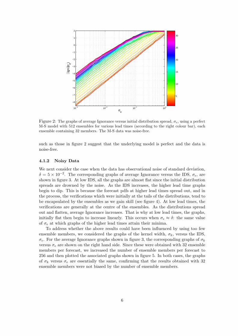
For the case δ = 0, the graphs of average Ignorance, 〈ign(σe)〉 , versus the IDS, σe, areshown in figure 2. The different colours correspond to the different lead times of upto 32 time steps. Notice that the graphs generally yield straight lines except at higherlead times and IDS. In particular, the magenta lines (corresponding to lead times of 32)saturate at higher values of σe. As the IDS increases, we would expect the forecast pdfsat low lead times to be approximately flattened Gaussians. That is why all the red lines(lead times 1 and 2) grow linearly without saturating. Notice that the lead times of, say31 and 32, score less than the 20 lead times when σe > 10−1. When higher lead timeforecasts score less than lower lead times, we say we have return of skill. Linear graphs

5

10−3

10−2

10−1

100

−8

−7

−6

−5

−4

−3

−2

−1

0

1

2

σe

⟨ ign

⟩(σe)

5

10

15

20

25

30

Figure 2: The graphs of average Ignorance versus initial distribution spread, σe, using a perfectM-S model with 512 ensembles for various lead times (according to the right colour bar), eachensemble containing 32 members. The M-S data was noise-free.

such as those in figure 2 suggest that the underlying model is perfect and the data isnoise-free.

4.1.2 Noisy Data

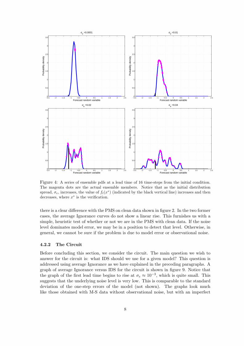
We next consider the case when the data has observational noise of standard deviation,δ = 5 × 10−2. The corresponding graphs of average Ignorance versus the IDS, σe, areshown in figure 3. At low IDS, all the graphs are almost flat since the initial distributionspreads are drowned by the noise. As the IDS increases, the higher lead time graphsbegin to dip. This is because the forecast pdfs at higher lead times spread out, and inthe process, the verifications which were initially at the tails of the distributions, tend tobe encapsulated by the ensembles as we gain skill (see figure 4). At low lead times, theverifications are generally at the centre of the ensembles. As the distributions spreadout and flatten, average Ignorance increases. That is why at low lead times, the graphs,initially flat then begin to increase linearly. This occurs when σe ≈ δ: the same valueof σe at which graphs of the higher lead times attain their minima.

To address whether the above results could have been influenced by using too fewensemble members, we considered the graphs of the kernel width, σk, versus the IDS,σe. For the average Ignorance graphs shown in figure 3, the corresponding graphs of σk

versus σe are shown on the right hand side. Since these were obtained with 32 ensemblemembers per forecast, we increased the number of ensemble members per forecast to256 and then plotted the associated graphs shown in figure 5. In both cases, the graphsof σk versus σe are essentially the same, confirming that the results obtained with 32ensemble members were not biased by the number of ensemble members.

6

10−3

10−2

10−1

100

−1.5

−1

−0.5

0

0.5

1

1.5

2

σe

⟨ ig

n⟩(

σe)

5

10

15

20

25

30

10−3

10−2

10−1

100

0.05

0.1

0.15

0.2

0.25

0.3

0.35

σe

σk (

Ke

rne

l wid

th)

5

10

15

20

25

30

Figure 3: (left) The graph of ignorance versus initial distribution spread, σe, for the perfect M-Smodel with 512 ensembles for various lead times (according to the right colour bar), each ensem-ble containing 32 members. Observational noise of standard deviation 5 × 10−2. (right) Graphof kernel width versus initial distribution spread. The vertical and horizontal thick dash-dottedlines correspond to the noise spread.

4.2 Imperfect Model Scenario

We now carry over the ideas of the preceding subsections to the IMS, considering modelsof the form

xn = φ(xn−1), (10)

where xn−1 is a delay vector. The deterministic model, φ, was built from data usingcubic radial basis functions.

4.2.1 The M-S system

Let us first consider M-S data with observational noise, δ = 10−2 and 10−1. The graphsof average Ignorance versus IDS, σe, for various lead times are shown in figure 6. Wenotice that the low lead time graphs begin to rise at σe ≈ δ. At a slightly larger value ofσe, graphs for the higher lead times reach their minima. This is very much reminiscentto the PMS, and suggests a way of using nonlinear prediction to detect noise level.

Suppose the noise of the underlying system is not Gaussian but is uniformly dis-tributed with standard deviation δ. We consider this case and the noise distributionto be U [−b, b], in which case δ2 = b2/3. We have plotted graphs of average Ignoranceversus IDS in figure 7 with δ = 10−1. Again we see graphs dipping at σe ≈ δ.

When the data is noise free, we have the results shown in figure 8. They are quali-tatively similar to the PMS and IMS with noisy data. This case also presents strikingdifferences from the previous noisy data scenarios. The optimal spread varies with leadtime as highlighted by the black solid line on the figure. In this case, one may select theIDS that yields good forecasting performance at higher lead times.

The foregoing discussions can be summarised as follows: Whereas there is similarityin the graphs of average Ignorance for the PMS with observational noise and the IMS,

7

−2.5 −2 −1.5 −1 −0.5 0 0.5 1 1.5 2 2.50

0.5

1

1.5

2

2.5

3

3.5

Pro

babi

lity

dens

ity

Forecast random variable

σe =0.0001

−2.5 −2 −1.5 −1 −0.5 0 0.5 1 1.5 2 2.50

0.5

1

1.5

2

2.5

3

3.5

Pro

babi

lity

dens

ity

Forecast random variable

σe =0.01

−2.5 −2 −1.5 −1 −0.5 0 0.5 1 1.5 2 2.50

0.5

1

1.5

2

2.5

3

3.5

Pro

babi

lity

dens

ity

Forecast random variable

σe =0.02

−2.5 −2 −1.5 −1 −0.5 0 0.5 1 1.5 2 2.50

0.5

1

1.5

2

2.5

3

3.5

Pro

babi

lity

dens

ity

Forecast random variable

σe =0.04

Figure 4: A series of ensemble pdfs at a lead time of 16 time-steps from the initial condition.The magenta dots are the actual ensemble members. Notice that as the initial distributionspread, σe, increases, the value of ft(x

∗) (indicated by the black vertical line) increases and thendecreases, where x∗ is the verification.

there is a clear difference with the PMS on clean data shown in figure 2. In the two formercases, the average Ignorance curves do not show a linear rise. This furnishes us with asimple, heuristic test of whether or not we are in the PMS with clean data. If the noiselevel dominates model error, we may be in a position to detect that level. Otherwise, ingeneral, we cannot be sure if the problem is due to model error or observational noise.

4.2.2 The Circuit

Before concluding this section, we consider the circuit. The main question we wish toanswer for the circuit is: what IDS should we use for a given model? This question isaddressed using average Ignorance as we have explained in the preceding paragraphs. Agraph of average Ignorance versus IDS for the circuit is shown in figure 9. Notice thatthe graph of the first lead time begins to rise at σe ≈ 10−3, which is quite small. Thissuggests that the underlying noise level is very low. This is comparable to the standarddeviation of the one-step errors of the model (not shown). The graphs look muchlike those obtained with M-S data without observational noise, but with an imperfect

8

10−3

10−2

10−1

100

−1.5

−1

−0.5

0

0.5

1

1.5

2

σe

⟨ ig

n⟩(

σe)

τp=1

τp=16

τp=32

10−3

10−2

10−1

100

0.05

0.1

0.15

0.2

0.25

0.3

0.35

0.4

0.45

0.5

0.55

σe

σk (

Ke

rne

l wid

th)

τp=1

τp=16

τp=32

Figure 5: (left) The graph of ignorance versus initial distribution spread, σe, for the perfectM-S model with 512 ensembles for three lead times, each ensemble containing 256 members.Observational noise had standard deviation 5 × 10−2. (right) Graph of kernel width versusinitial distribution spread. The vertical and horizontal thick dash-dotted lines correspond to thenoise spread.

10−3

10−2

10−1

−4

−3

−2

−1

0

1

2

σe

⟨ ig

n⟩(

σe)

10

20

30

40

50

60

10−3

10−2

10−1

−0.5

0

0.5

1

1.5

2

σe

⟨ ig

n⟩(

σe)

10

20

30

40

50

60

Figure 6: Graphs of average Ignorance versus logarithmically initial distribution spread, σe,with observational error of standard deviation δ = 10−2 (left) and 10−1 (right) on M-S datawith an imperfect model. 128 initial conditions with a time step of 64 between them were used.Each initial ensemble containing 32 members was iterated forward up to 64 time steps. Themultiple lines correspond to different lead times. The lowest lines correspond to the lowest leadtimes but there is a mixing up of higher lead times at the top of each graph. The vertical thickdash-dotted lines correspond to the noise spread.

model (see figure 8), albeit without dipping to such an extent.

9

10−3

10−2

10−1

−0.5

0

0.5

1

1.5

2

σe

⟨ ign

⟩(σe)

10

20

30

40

50

60

Figure 7: Graphs of Ignorance versus logarithmically varying initial distribution spread, σe,of ensemble perturbations with uniformly distributed observational error of standard deviationδ = 10−1 on M-S data with an imperfect model. 128 initial conditions with a time step 64between them were used. 32 initial ensembles were generated in each and iterated forward upto 64 time steps. The multiple lines correspond to different lead times according to the colourbar on the right. The vertical thick dash-dotted line corresponds to the noise spread.

4.3 Theoretical Considerations

To explain the previous observations, we consider two pdfs of the perfect forecast andthe imperfect forecasts: pt(x;σp, µp) and ft(x;σf , µf ), where σp (or σf ) and µp (or µf )are the standard deviation and mean respectively of pt (or ft), assuming that

σp(t) = hp(σe, t) and σf (t) = hf (σe, t).

Suppose our forecast, ft, is Gaussian 2, so that

ft(x;σf , µf ) =1

σf

√2π

e−(x−µf )2/2σ2

f .

Then the expected skill of ft is

E[ign(ft,X)] = −∫

∞

−∞

pt(x;σ2p , µp) log ft(x;σ2

f , µf )dx

=1

2log(2πσ2

f ) +σ2

p

2σ2f

+1

2σ2f

(µp − µf )2. (11)

We assume that the standard deviations, σp and σf , are monotonic increasing functionsof σe. If σp = σf then (11) reduces to

E[ign(ft,X)] =1

2log(2πeσ2

f ) +1

2σ2f

(µp − µf )2 (12)

2Operationally, this may not be the case.

10

10−3

10−2

10−1

−6

−5

−4

−3

−2

−1

0

1

2

3

σe

⟨ ign

(σe)⟩

5

10

15

20

25

30

Figure 8: The graphs of average Ignorance versus initial distribution spread with 512 ensembles,each ensemble containing 32 members and using a cubic rbf model on noise free M-S data. Thecolour bar on the right shows the lead times for the different graphs of Ignorance. The solidblack line indicates where the global minimum occurs for each graph. Notice how the optimumspread varies with lead time.

and the expected skill is minimised by

σf = |µp − µf |. (13)

If, in addition, µp = µf , then

E[ign(ft,X)] =1

2log(2πeσ2

f ), (14)

which is a monotonically increasing function of σf . This may explain why straightline graphs were obtained in the noise free PMS. They arise when the perfect and theimperfect forecast ensembles have equal means and variances.

If µp 6= µf , then the expected skill has a global minimum given by

minσf >0

E[ign(ft,X)] =1

2log

[

2πe2(µp − µf )2]

. (15)

In particular,

minσe>0

E[ign(f0,X)] =1

2log

[

2πe2ξ20

]

, (16)

where ξ0 = µp − µf ∼ N(0, δ2). Here, µp is the mean of the initial distribution fromwhich the initial condition, x0, was drawn and µf is the mean of the forecast pdf. Theinitial condition lies on the attractor. For a more general case, at lead time t, we defineξt = µp(t) − µf (t). If σe > ξ0, then the minimum in (16) will not be attained by

11

10−4

10−3

10−2

10−1

−7

−6

−5

−4

−3

−2

−1

0

1

σe

⟨ ign

(σe)⟩

5

10

15

20

25

30

Figure 9: Graphs of average Ignorance versus logarithmically varying initial distribution spread,σe, on circuit data. 512 initial conditions with a time step of 64 between them were used. Eachinitial ensemble containing 32 members was iterated forward up to 32 time steps. The multiplelines correspond to different lead times according to the colour bar on the right.

increasing σe because it can only be attained when σf = σe = |ξ0|. However, over awindow of time series, the average may be constant for a while as witnessed in figure 3.We assume that for t close to zero, the distribution of ξt is approximately that of ξ0.For higher lead times, the minima of the average skill are attained at σe = δ.

5 Discussion

The computational results presented in this paper demonstrated a way to select thespread of the distribution from which to sample an initial ensemble of points. Thegoal was to obtain an initial ensemble that would minimise uncertainty in the forecastdistributions. The forecasting model need not be perfect for the method to be applied.Information theoretic approaches were used to obtain the computational results andjustify them. The methodology is a departure from traditional data assimilation andensemble forecasting techniques in a number of ways. We recognise that the ultimategoal of any method that estimates an initial distribution is to obtain more accurateforecasts.

Data assimilation techniques either focus on estimating the true state of the system ora set of such estimates. To this end, a model trajectory may be sought that is consistentwith observations [2, 25]. It is believed that forecasts made from an ensemble that liesalong such trajectories would provide good forecasts. An ensemble of trajectories isobtained by making perturbations of some initial observation. When there is modelerror, there is no model trajectory that is consistent with observations. Therefore,Judd and Smith [5] talk of pseudo-orbits instead. Notwithstanding these difficulties,

12

the method presented here could be used to determine the spread of this distribution,regardless of the data assimilation technique. For a given structure of the correlationmatrix, we would seek the scalar multiple that yields the most informative forecastdistributions.

Other techniques for producing the initial ensemble aim at selectively sampling thosepoints that are dynamically the most relevant. In particular, the ECMWF ensembleprediction system seeks perturbations of the initial state based on the leading singularvectors of the linear propagator [1]. This approach can lead to over-confidence whenthere is model error. One falls into the trap of confusing the dynamics of the modelwith those of the underlying system as highlighted in [26]. To safeguard this problem,our methodology may be used to select the IDS.

The results also suggest that the method may be useful in nonlinear noise reduction.For nonlinear noise reduction, the quality of the model would have to be very good,at least in the sense of forecasting. However, the primary value of the method is tofind the spread of the initial distribution. It is also interesting that even when there isno observational noise, sampling the initial distribution could still help mitigate modelinadequacy.

Finally, possible areas of application go beyond meteorology and the Geo-sciences.For instance, evidences of nonlinear dynamics have already been reported in economicsand finance [27]. In some cases these dynamics are fairly low dimensional (e.g. [28]), thusreducing the computational costs that may arise from generating an initial ensemble. Weenvision the method being of great value in these disciplines to tackle density forecasting.

6 Conclusions

This paper argued for combining the task of choosing the initial ensemble with densityforecasting. The point is that, when faced with model error, a knowledge of the truestate of the system is irrelevant because it cannot provide one with a perfect forecast.Moreover, using the true state with an imperfect model can provide forecasts that arefurther from the truth than forecasts obtained with imperfect initial states. Therefore,it has been argued that the task of the forecaster should be to choose initial distri-butions that yield the most informative forecast distributions. Whereas this approachmay be incorporated into traditional ensemble forecasting techniques, it can also standindependently as a forecasting method.

To recap, it was demonstrated that the logarithmic scoring rule can be used toestimate an optimum IDS for a given system and model. At the optimal spread, higherlead time graphs of the logarithmic scoring rule versus IDS tend to dip. Although itis critical that we use Gaussian initial distributions, the distribution of the underlyingobservational uncertainty or model error seems not to play a crucial role. It turnsout that we can also diagnose the fictitious case of a perfect model with perfect initialstates. A theoretical explanation for the empirical observations regarding the dipping ofthe graphs has been presented. Also, by appealing to ergodicity, the theoretical score hasalso been related to the empirical score. It is noteworthy that Bernardo’s theorem [29]states that the logarithmic score is the only proper, local scoring rule. This point shoulddispel concern about the generality of the results.

13

Acknowledgements

The authors would like to thank Leonard A. Smith, Devin Kilminster and membersof the Applied Dynamical Systems Group at Oxford for fruitful discussions and usefulinsights. This work was supported by the Commonwealth scholarship, the LSE’s HigherEducation Infrastructure fund and the RCUK Digital Economy Programme fund at theUniversity of Reading.

References

[1] M. Leutbecher, T. N. Palmer, Ensemble Forecasting, Journal of ComputationalPhysics 227 (2008) 3515–3539.

[2] K. Judd, L. A. Smith, Indistinguishable states I: Perfect model scenario, PhysicaD 151 (2001) 125–141.

[3] L. M. Stewart, Correlated observation errors, Ph.D. thesis, University of Reading(2010).

[4] A. Hollingsworth, P. Lonnberg, The statistical structure of short-range forecasterrors as determined from radiosonde data. part 1: The wind field, Tellus 38A(1986) 111–136.

[5] K. Judd, L. A. Smith, Indistinguishable states II: The imperfect model scenario,Physica D 196 (2004) 224–242.

[6] L. A. Smith, C. Ziehman, K. Fraedrich, Uncertainty in dynamics and predictabilityin chaotic systems, Q. J. R. Meteorol. Soc. 125 (1999) 2855–2886.

[7] M. S. Roulston, L. A. Smith, Combining dynamical and statistical ensembles, Tellus55A (2003) 16–30.

[8] J. Broecker, L. A. Smith, From Ensemble Forecasting to Predictive DistributionFunctions, Tellus A 60 (2008) 663.

[9] E. Parzen, On the Estimation of a Probability Density Function and Mode, TheAnnals of Mathematical Statistics 33 (1962) 1065–1076.

[10] B. W. Silverman, Density Estimation for Statistics and Data Analysis, 1st Edition,Chapman and Hall, 1986.

[11] I. J. Good, Rational decisions, Journal of the Royal Statistical Society. Series B(Methodological) 14 (1952) 107–114.

[12] M. S. Roulston, L. A. Smith, Evaluating Probabilistic Forecasts Using InformationTheory, Monthly Weather Review 130 (2002) 1653–1660.

[13] A. I. Khinchin, Mathematical Foundations of Information Theory, 1st Edition,Dover Publications, Inc., 1957.

[14] C. E. Shannon, A Mathematical theory of communication, Bell Systems TechnologyJournal 27 (1948) 379–423,623–656.

14

[15] J. Broecker, U. Parlitz, M. Ogorzalek, Nonlinear noise reduction, Proc. of the IEEE90.

[16] W. D. Moore, E. A. Spiegel, A thermally excited nonlinear oscillator, The Astro-physical Journal 143 (1966) 871–887.

[17] L. O. Chua, Experimental chaos synchronisation in Chua’s circuit, InternationalJournal of Bifurcation and Chaos 2 (1992) 704.

[18] M. I. Gorlov, A. V. Strogonov, ARIMA Models Used to Predict the Time to Degra-dation Failure of TTL IC’s, Russian Microelectronics 36 (2007) 261–270.

[19] E. A. Coddington, N. Levinson, Theory of Ordinary Differential Equations, NewYork:McGraw-Hill, 1955.

[20] E. Ott, T. Sauer, J. A. Yorke (Eds.), Coping With Chaos: Analysis of chaotic dataand the exploitation of chaotic systems, John Wiley and Sons Inc., 1994.

[21] J. Broecker, L. A. Smith, Scoring Probabilistic Forecasts: The importance of beingproper, Weather and Forecasting 22 (2007) 382–388.

[22] T. Gneiting, A. E. Raftery, Strictly proper scoring rules, prediction and estimation,J. Amer. Math. Soc. 102 (2007) 359–378.

[23] K. Judd, A. Mees, On selecting models for nonlinear time series, Physica D. 82(1995) 426–444.

[24] R. L. Machete, Modelling a Moore-Spiegel Electronic Circuit: the imperfect modelscenario, DPhil Thesis, University of Oxford (2008).

[25] G. Burgers, P. J. van Leeuwen, G. Evensen, Analysis scheme in the ensemble kalmanfilter, Monthly Weather Review 126 (1998) 1719–1724.

[26] L. A. Smith, Chaos: A Very Short Introduction, 1st Edition, Oxford UniversityPress, 2007.

[27] T. Terasvirta, Forecasting Economic Variables with Nonlinear Models, in: G. El-liott, C. W. J. Granger, A. Timmermann (Eds.), Handbook of Economic Forecast-ing, Vol. 1, North-Holland, 2006.

[28] N. Linden, S. Satchell, Y. Yoon, Predicting British Financial Indices: An approachbased on chaos theory, Structural Change and Economic Dynamics 4.

[29] J. M. Bernardo, Expected information as expected utility, Annals of Statistics 7(1979) 686–690.

[30] J.-P. Eckmann, D. Ruelle, Ergodic theory of chaos and strange attractors, Rev.Mod. Phys. 57 (1985) 617–653.

15

A Invariant Density

Associated with the attractor A is some invariant measure [30], , such that

[ϕ−t(E)] = (E), (17)

where E ⊂ Rm is a measurable set and ϕ

−t(E) is the set obtained by evolving eachpoint in E backwards in time. A probability measure on E may be defined as [30]

(E) = limT→∞

1

T

∫ T

01E(ϕt(x0))dt, (18)

where 1E is an indicator function 3. Provided the attractor A is ergodic 4,

(E) =

∫

E(dx). (19)

Associated with is some probability density function, ρ, such that (19) may be rewrit-ten as

(E) =

∫

Eρ(x)dx. (20)

We call ρ(x) the invariant density of the attractor A or the flow ϕt(x0). This invariantdensity is indeed the climatology 5 mentioned in the introduction.

3An indicator is defined by

1E(x) =

1 if x ∈ E,

0 if x 6∈ E.

4In an ergodic attractor, state space averages are equal to time averages [30].5Including its marginal densities.

16