derivatives performance attribution 2 derivatives performance attribution c=f(s,t) u d subsequent...

1

Derivatives Performance Attribution1

C=f(S,t)

u

d

Derivatives PerformanceAttribution

Mark RubinsteinPaul Stephens Professor of Applied Investment Analysis

University of California at [email protected]

Abstract

This paper shows how to decompose the dollar profit earned from an option into two basic components:

¶ mispricing of the option relative to the asset at the time of purchase, and· profit from subsequent fortuitous changes or mispricing of the underlying asset.

This separation hinges on measuring the “true relative value” of the option from its realized payoff. Thepayoff from any one option has a huge standard error about this value which can be reduced byaveraging the payoff from several independent option positions. It appears from simulations that 95%reductions in standard errors can be further achieved by using the payoff of a dynamic replicatingportfolio as a Monte Carlo control variate. In addition, it is shown that these low standard errors arerobust to discrete rather than continuous dynamic replication and to the likely degree of misspecificationof the benchmark formula used to implement the replication.

The first basic component, the option mispricing profit, can be further decomposed into profit due tosuperior estimation of the volatility (volatility profit) and profit from using a superior option valuationformula (formula profit). In order to make this decomposition reliably, the benchmark formula used forthe attribution needs to be similar to the formula implicitly used by the market to price options. If so,then simulation indicates that this further decomposition can be achieved with low standard errors.

The second basic component can be further decomposed into profit from a forward contract on theunderlying asset (asset profit) and what I term pure option profit. The asset profit indicates whether ornot the investor was skillful by buying or selling options on mispriced underlying assets. However, assetprofit could also simply be just compensation for bearing risk -- a distinction beyond the scope of thispaper. Although simulation indicates that the attribution procedure gives an unbiased allocation of theoption profit to this source, its standard error is large -- a feature common with attempts by others tomeasure performance of assets.

May 3, 1998

Mark Rubinstein is the Paul Stephens Professor of Applied Investment Analysis at the University ofCalifornia at Berkeley. The author would like to thank Barra, Inc. for encouraging this research.

2


C=f(S,t)

u

d

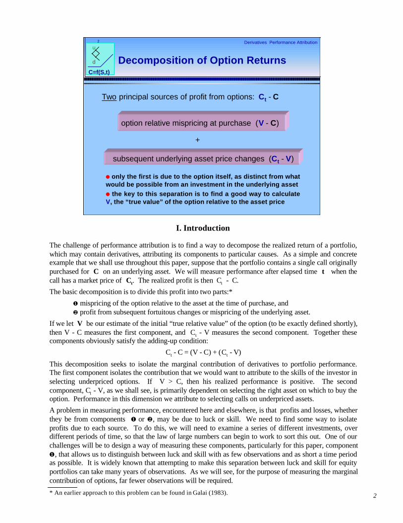
subsequent underlying asset price changes (Ct - V)

Two principal sources of profit from options: Ct - C

l only the first is due to the option itself, as distinct from whatwould be possible from an investment in the underlying assetl the key to this separation is to find a good way to calculateV, the “true value” of the option relative to the asset price

+

Decomposition of Option Returns

option relative mispricing at purchase (V - C)

I. Introduction

The challenge of performance attribution is to find a way to decompose the realized return of a portfolio,which may contain derivatives, attributing its components to particular causes. As a simple and concreteexample that we shall use throughout this paper, suppose that the portfolio contains a single call originallypurchased for C on an underlying asset. We will measure performance after elapsed time t when thecall has a market price of Ct. The realized profit is then Ct - C.

The basic decomposition is to divide this profit into two parts:*

¶ mispricing of the option relative to the asset at the time of purchase, and· profit from subsequent fortuitous changes or mispricing of the underlying asset.

If we let V be our estimate of the initial “true relative value” of the option (to be exactly defined shortly),then V - C measures the first component, and Ct - V measures the second component. Together thesecomponents obviously satisfy the adding-up condition:

Ct - C = (V - C) + (Ct - V)

This decomposition seeks to isolate the marginal contribution of derivatives to portfolio performance.The first component isolates the contribution that we would want to attribute to the skills of the investor inselecting underpriced options. If V > C, then his realized performance is positive. The secondcomponent, Ct - V, as we shall see, is primarily dependent on selecting the right asset on which to buy theoption. Performance in this dimension we attribute to selecting calls on underpriced assets.

A problem in measuring performance, encountered here and elsewhere, is that profits and losses, whetherthey be from components ¶ or ·, may be due to luck or skill. We need to find some way to isolateprofits due to each source. To do this, we will need to examine a series of different investments, overdifferent periods of time, so that the law of large numbers can begin to work to sort this out. One of ourchallenges will be to design a way of measuring these components, particularly for this paper, component¶, that allows us to distinguish between luck and skill with as few observations and as short a time periodas possible. It is widely known that attempting to make this separation between luck and skill for equityportfolios can take many years of observations. As we will see, for the purpose of measuring the marginalcontribution of options, far fewer observations will be required.

* An earlier approach to this problem can be found in Galai (1983).

3


C=f(S,t)

u

dFurther Decomposition of OptionReturns

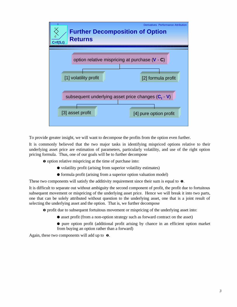
[1] volatility profit [2] formula profit

[3] asset profit [4] pure option profit

option relative mispricing at purchase (V - C)

subsequent underlying asset price changes (Ct - V)

To provide greater insight, we will want to decompose the profits from the option even further.

It is commonly believed that the two major tasks in identifying mispriced options relative to theirunderlying asset price are estimation of parameters, particularly volatility, and use of the right optionpricing formula. Thus, one of our goals will be to further decompose

¶ option relative mispricing at the time of purchase into:

l volatility profit (arising from superior volatility estimates)

l formula profit (arising from a superior option valuation model)

These two components will satisfy the additivity requirement since their sum is equal to ¶.

It is difficult to separate out without ambiguity the second component of profit, the profit due to fortuitoussubsequent movement or mispricing of the underlying asset price. Hence we will break it into two parts,one that can be solely attributed without question to the underlying asset, one that is a joint result ofselecting the underlying asset and the option. That is, we further decompose

· profit due to subsequent fortuitous movement or mispricing of the underlying asset into:

l asset profit (from a non-option strategy such as forward contract on the asset)

l pure option profit (additional profit arising by chance in an efficient option marketfrom buying an option rather than a forward)

Again, these two components will add up to ·.

4


C=f(S,t)

u

d Three Formulas

n “true formula”: the option valuation formula based on theactual risk-neutral stochastic process followed by theunderlying assetn “market’s formula”: the option valuation formula used bymarket participants to set market pricesn benchmark formula: the option valuation formula used inthe process of performance attribution to

(1) help determine the “true relative value” of the option(2) decompose option mispricing profit into components

We distinguish between these formulas and their riskless return andvolatility inputs, for which there are also three estimates -- true, market,and benchmark. Essentially, by the “formula” we mean the levels of allthe other higher moments of the risk-neutral distribution, where eachmoment may possibly depend on the input riskless return and volatility.

We will need to distinguish between three option valuation formulas. The “true formula” captures theactual risk-neutral stochastic process of the underlying asset price. Although we do not know thisformula, we can hope to learn something about it by observing the realized option payoffs. Usingsimulation in Part IV of this paper, the performance attribution approach does not generally know whatthe true formula is. But, since the simulation itself will know the true formula, we can ask how quicklyour performance attribution method learns about this formula.

To separate components of performance, we also need to know the formula used by the market in settingoption prices, which we call the “market’s formula”. In an inefficient market, this may not coincidewith the “true formula”.

A third formula, used directly in the methodology, is called the benchmark formula, such as the standardbinomial option pricing model. We will use the benchmark formula for two purposes:

(1) to help determine the “true relative value” V of the option

(2) to decompose the profit due to option mispricing into components

For the first, we will want to use a benchmark formula that comes as close as possible to the “trueformula.” For the second, we want a benchmark formula that comes as close as possible to the “market’sformula.” In particular, if the market uses the wrong formula, the same formula will not satisfy both thesepurposes, so more generally we would want to consider using different benchmark formulas for eachpurpose. It is one thing to hope we understand how the market values options, but it is quite another toknow the “true formula” if this is different. So, in this paper, we will use the same formula -- our bestguess about the “market’s formula” -- for both purposes.

Fortunately, as we shall see, even if our benchmark formula is a poor approximation of the “market’sformula,” our calculation of V may not be seriously affected since it can be cured by the law of largenumbers. However, failure to use the “market’s formula” will affect the way we decompose optionmispricing profit and will not be cured by a large sample.

In this paper, we will use the standard binomial model as the benchmark formula. But in practicalapplications we may prefer using the constant elasticity of variance, jump-diffusion, or an impliedbinomial tree model depending on the nature of the stochastic process of the underlying asset and ourbeliefs about how the market prices options.

5


C=f(S,t)

u

d

n Payoff attributed to difference between the realized (s) andimplied volatility at purchase based on benchmark formula:

C(s) - C

n Positive results indicate that the investor was cleverenough to buy options in situations where the marketunderestimated the forthcoming volatility.

[1] Volatility Profit

(Caveat: Although we can know that an option is mispriced, we will notbe able to tell why it is mispriced if the benchmark formula used tocalculate C(s) is not a good approximation of the formula used by themarket to set the option price C.)

The profit from option relative mispricing at purchase V - C,can be decomposed into 2 parts:

II. Four Components of Performance

No doubt our attempt to describe this decomposition of option profit in succinct English is not as clear asone would like. So now, with the aid of mathematics, we take each of the components up one by one.

Profit results if an investor can successfully identify mispriced options. We will decompose this basiccomponent of profit into two parts: profit made because the investor was good at predicting volatility andprofit made because the investor was good at finding a superior option valuation formula to the oneapparently used by the market, reflected in the initial market price of the option. Academic research thatinvestigates how well a model’s implied volatility forecasts realized volatility concerns itself with the firstof these. Whereas academic research that focuses on how well alternative option pricing models forecastfuture option prices, conditional on the future underlying asset price, is primarily concerned with thesecond of these.

To isolate the profits made from superior forecasts of volatility, we calculate the initial value the optionshould have had, using the benchmark formula, had the realized volatility of the asset over the assessmentperiod (elapsed time t) been known in advance. We use s to represent annualized realized volatilityover the assessment period. It is not immediately clear how this should be measured, but a first cut is tomeasure the sample volatility of realized daily asset returns. The value of the option measured by thebenchmark option pricing formula with volatility parameter s is denoted by C(s). In contrast, the currentoption price C can be interpreted as the value of the option measured by the benchmark option pricingformula with volatility parameter σ, which is the implied volatility. So we can interpret the difference,volatility profit,

C(s) - C

as the mispricing of the option due to the fact that under the benchmark formula, the market mistakenlythought that the volatility was σ rather than the volatility s that actually was realized.

If this is positive, it suggests that the investor may have skill in forecasting volatility.

6


C=f(S,t)

u

d

n Profit attributed to using a formula superior to thebenchmark formula, assuming realized volatility were knownin advance:

V - C(s)

n Positive results indicate that the investor was cleverenough to buy options for which the benchmark formula,even with foreknowledge of the realized volatility,undervalued the options.

[2] Formula Profit

(Caveat: Although we can know that an option is mispriced, we will notbe able to tell why it is mispriced if the benchmark formula used tocalculate C(s) is not a good approximation of the formula used by themarket to set the option price C.)

It is important to realize that our measure of volatility profit can be quite sensitive to the benchmarkformula. For this purpose, we want to choose as a benchmark our best guess for the formula used by themarket to price options. If the benchmark is incorrect, then we will mistakenly confuse volatility profitwith formula profit. If we do not know the market’s formula, then although we can know that an optiontends to be mispriced, we will not be able to tell why it is mispriced.

The second mispricing component isolates the profit from using an option pricing formula superior to thebenchmark. If V is the relative value of the option based not only on the true formula but also on therealized volatility, then the difference we call the formula profit,

V - C(s)

is the profit due to using a superior option valuation formula to the benchmark. Since both V and C(s)are measured using the realized volatility, this difference isolates the role of the option pricing formulafrom skill in forecasting volatility.

Again, for this decomposition to work, we need to be using a benchmark that is a good approximation forthe formula used by the market to set the option price C.

Note: In practice, to reduce the standard error of the decomposition of option mispricing into volatility and formulaprofits, we will average the calculations over several option investments. Averaging C(s) – the benchmark formulavalues based on realized volatility – produces a biased estimate because the formula value is generally a non-linearfunction of the volatility. However, using benchmark formulas similar to Black-Scholes induces a trivial bias sincethis formula is almost linear in volatility over the relevant range. For example, using the parameter inputs we willlater use in our simulation, at-the-money European calls using the Black-Scholes formula have the following valuesassociated with their annualized volatility:

volatility option value

15% $2.7509

20% $3.5549

25% $4.3599

Given the option values at 15% and 25% volatilities, if the formula were exactly linear in volatility, then the optionvalue at 20% volatility would be $3.5553.

7


C=f(S,t)

u

d

n Payoff from an otherwise identical forward contract:

St - S(r/d)t

n Positive results indicate that the investor may be good atselecting the right underlying asset.

[3] Asset Profit

(In an efficient market with risk neutrality, asset profit will tend to bezero. Thus, if it tends to be positive or negative, either this must becompensation for risk or indicative of an inefficient asset market -- adistinction we must leave to others.)

The profit from subsequent underlying asset price changesCt - V, can be decomposed into 2 parts:

The next component of profit is simply the performance of a benchmark strategy, assumed to be a forwardcontract on the underlying asset, which we call the asset profit:

St - S(r/d)t

where:S is the price of the asset at the time the option was purchasedSt is the price of the asset after elapsed time t (when performance is being assessed)r is the annualized riskless return over the periodd is the annualized payout return over the period for the asset

r and d are two parameters, along with volatility, that determine the value of options.*

S(r/d)t is the formula for the fair value of a forward contract on the asset with a time-to-delivery of t.Therefore, the difference St - S(r/d)t is the realized profit from this forward contract. In an efficient assetmarket, the present value of this is zero.

Note that the choice of the benchmark strategy is to some extent arbitrary. Another benchmark couldeasily be used instead. The benchmark hides the factors that will be unexplained by our analysis. Whileour calculation St - S(r/d)t measures the profit from selecting the asset underlying the option, in thispaper we will not in turn decompose that into its sources -- a problem which has many commerciallyavailable solutions.

In an efficient asset market with risk neutrality, the asset profit will on average be zero. If it tends to beunequal to zero, then either the market is risk averse (or risk preferring) or the underlying asset ismispriced. This is not a distinction which this paper can help sort out.

* While we assume that the true volatility is not known by the investor in advance, to simplify the paper and addressthe most important sources of option profit, we assume that r and d are known in advance.

8


C=f(S,t)

u

d

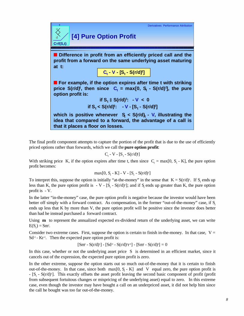
n Difference in profit from an efficiently priced call and theprofit from a forward on the same underlying asset maturingat t:

Ct - V - [St - S(r/d)t]

n For example, if the option expires after time t with strikingprice S(r/d)t, then since Ct = max[0, St - S(r/d)t], the pureoption profit is:

if St ≥ S(r/d)t: - V < 0if St < S(r/d)t: - V - [St - S(r/d)t]

which is positive whenever St < S(r/d)t - V, illustrating theidea that compared to a forward, the advantage of a call isthat it places a floor on losses.

[4] Pure Option Profit

The final profit component attempts to capture the portion of the profit that is due to the use of efficientlypriced options rather than forwards, which we call the pure option profit:

Ct - V - [S t - S(r/d)t]

With striking price K, if the option expires after time t, then since Ct = max[0, St - K], the pure optionprofit becomes:

max[0, St - K] - V - [St - S(r/d)t]

To interpret this, suppose the option is initially “at-the-money” in the sense that K = S(r/d) t. If St ends upless than K, the pure option profit is - V - [St - S(r/d)t]; and if St ends up greater than K, the pure optionprofit is - V.

In the latter “in-the-money” case, the pure option profit is negative because the investor would have beenbetter off simply with a forward contract. As compensation, in the former “out-of-the-money” case, if St

ends up less that K by more than V, the pure option profit will be positive since the investor does betterthan had he instead purchased a forward contract.

Using m to represent the annualized expected ex-dividend return of the underlying asset, we can writeE(St) = Smt.

Consider two extreme cases. First, suppose the option is certain to finish in-the-money. In that case, V =Sd-t - Kr-t. Then the expected pure option profit is:

[Smt - S(r/d)t] - [Sd-t - S(r/d)tr-t] - [Smt - S(r/d)t] = 0

In this case, whether or not the underlying asset price S is determined in an efficient market, since itcancels out of the expression, the expected pure option profit is zero.

In the other extreme, suppose the option starts out so much out-of-the-money that it is certain to finishout-of-the-money. In that case, since both max[0, St - K] and V equal zero, the pure option profit is- [St - S(r/d)t]. This exactly offsets the asset profit leaving the second basic component of profit (profitfrom subsequent fortuitous changes or mispricing of the underlying asset) equal to zero. In this extremecase, even though the investor may have bought a call on an underpriced asset, it did not help him sincethe call he bought was too far out-of-the-money.

9


C=f(S,t)

u

d

[1] C(s) - C (volatility profit) + [2] V - C(s) (formula profit) + [3] St - S(r/d)t (asset profit) + [4] Ct - V - [St - S(r/d)t] (pure option profit)

Adding-Up Constraint

For efficiently priced options: C = E[V]If options are also correctly benchmarked:

E[C(s) - C] = E[V - C(s)] = 0For efficiently priced assets: PV[St - S(r/d)t] = 0

Ct - C =

The attached picture summarizes our decomposition of option profit. The profit of the option equals:

[1] [2] [3] [4]

volatility profit + formula profit + asset profit + pure option profit

For efficiently priced options, on average [1] + [2] = 0, whether or not the benchmark formula closelyapproximates the formula the market uses to value options.

If, in addition to the option being efficiently priced, the benchmark formula captures the market’s approachto option valuation, then on average [1] is zero and on average [2] is zero.

On any one option investment, due to sampling error, the realized volatility will be different than the truepopulation volatility, so C(s) ≠ C, but on average (ignoring slight nonlinearity effects), C(s) = C.

If the benchmark formula approximates the market’s formula, for inefficiently priced options, the magnitudeof [1] should on average indicate the value of an investor’s ability to make superior volatility forecasts, andthe magnitude of [2] should isolate on average the extent an investor is using a superior formula to themarket’s formula.

For efficiently priced assets, the present value of [3] should be zero while its magnitude indicatesappropriate compensation for bearing risk. For inefficiently priced assets, its present value will not be zeroand measures the extent an investor is skillful in selecting options with inefficiently priced underlyingassets.

For efficiently priced assets, the present value of [4] equals zero.

10


C=f(S,t)

u

d

V ≡ r-tE(Ct)

n One way to approximate V is to measure r-tCt. This isunbiased but will converge to V slowly, and also presumesrisk neutrality.

Definition of “True Relative Value”

n Instead use control variate Ct(S…St):

V ≡ r-tCt + [C - r-tCt(S…St)]

n Ct(S…St) is the amount in an account after elapsed timet of investing C on the purchase date in a self-financingdynamic replicating portfolio, where the implied volatility isused in the benchmark formula to estimate delta.

III. Estimating the “True Relative Value” of the Option

The trick to separating option mispricing profit from profit due to fortuitous underlying asset pricemovements or asset mispricing is to find some way to estimate the “true relative value” V of the option.

In an efficient market for the asset, ignoring risk aversion, V ≡ r- tE(Ct). So one way to estimate V wouldsimply be to observe a single r-tCt. Any one r-tCt would overstate or understate V. But over manyrealizations of sample paths for the underlying asset, V would be approximated by the average outcomefor r-tCt over these paths.

One problem with this simple Monte Carlo approach is that it may take a very large number of realizedsample paths for the average outcome of r-tCt to come close to V. We want to be able to measure theperformance of the investor more quickly. A way to speed up the process is to use a control variate.

Let Ct(S…St) be the amount in an account after elapsed time t from investing C on the purchase datein a portfolio comprised of the underlying asset and cash, and then subsequently attempting to replicatedynamically (with self-financing) the payoff of a call option with the same time-to-expiration and strikingprice as the purchased option. The option is replicated by using the benchmark formula together with theimplied volatility to estimate the delta. In practice, it may be sufficient in most markets to assume dailyrebalancing at the close to correct the delta. The realized difference Ct - Ct(S…St) measures the extentby which the benchmark formula, using the implied volatility, fails to replicate the option.

The natural control variate is the value of the replicating portfolio Ct(S…St), so that

V ≡ C + r- t[Ct - Ct(S…St)]Although, I refer to Ct(S…St) as a “control variate,” in real life application, it is simply the result ofrunning a parallel paper replicating portfolio for each option position under analysis.Note: One might have thought that a better replicating strategy for our purpose would have been to base thestrategy on the realized volatility along the sample path, rather than the beginning implied volatility. Unfortunately,this can lead to biased measures of value. For example, suppose the true stochastic process implies that realizedvolatility is inversely correlated with asset price. Then knowing at the beginning that the realized volatility will behigh leads one to expect a decline in the asset price. This information could then be used to almost assure thatCt(S…St) > Ct, along every path with the given realized volatility.

11


C=f(S,t)

u

d


simplifying : V* ≡ r-tCt and C* ≡ r-tCt(S…St)

Var(V) = Var(V*) + Var(C*) - 2 Cov(V*,C*)

The Monte Carlo Logic

Suppose that Var(V*) = Var(C*), then

Var(V) = 2 [Var V*] [1 - ρ(V*,C*)]

Suppose that ρ(V*,C*) = .9 (a fair benchmark), then

Var(V) = .2[Var(V*)]

To see why the proposed measure V ≡ r-tCt + [C - r- tCt(S…S t)] compares favorably to V ≡ r- tCt, simplifythe notation and set

V* ≡ r-tCt

C* ≡ r-tCt(S…St)]

So we have:

V = V* + [C - C*]

Taking variances of both sides:

Var(V) = Var(V*) + Var(C*) - 2 Cov(V*,C*)

To get a rough idea of the magnitudes involved, to a first approximation we could well expect

Var(V*) = Var(C*)

After all, in a Black-Scholes world of continuous trading, by using Black-Scholes also as the benchmarkformula, V* is exactly equal to C*. In that case, this approximation is exact.

Then, we can simplify to get:

Var(V) = 2 Var(V*) [1 - ρ(V*,C*)]

where ρ(V*, C*) is the correlation coefficient measuring association between V* and C*.

Experience with replicating strategies suggests that if the benchmark formula is Black-Scholes and thevolatility is implied, the benchmark-replicating strategy C* might be expected to produce outcomeshighly correlated with the realized option payoff. In light of this, assume that ρ(V*,C*) = .9. In thatcase,

Var(V) = .2 Var(V*)

This shows why, for this purpose, we want to use a benchmark formula that has the highest ρ(V*,C*).

Since Var(V) is much smaller than Var(V*), we can afford to use a much smaller sample to estimate Vthan V*. This translates into being able to identify ability to select mispriced options much more quickly.

12


C=f(S,t)

u

d

(1) V ≡ r-tCt

vs(2) V ≡ r-tCt + [C - r-tCt(S…St)]

An Additional Benefit

To see this, if S (or r) is too low, then Ct will tend to includeasset mispricing effects and be high. But Ct(S…St) will alsobe high (since it requires buying the asset and borrowing).This will tend to offset leaving V - C unchanged.

In an inefficient asset market, we hope that V will still serveto separate volatility and formula profit from asset profit.

Definition (1) does not do this. But definition (2) does.

Recall that we have defined the “true relative value” as:


What happens to V if the market misprices the underlying asset itself at the purchase of the option, butwe assume the asset is correctly priced at the end of the assessment period? In that case, had we simplydefined

V ≡ r-tCt

we would have a problem. Then, in a risk-neutral market, since on average V = r-tE(Ct) and Ct wouldreflect the correct asset price (which is the realized asset price at expiration), V would then be the “trueabsolute value” of the option inclusive of asset mispricing. This would be unfortunate for our purposessince we are hoping to use V to separate the effects of option mispricing (volatility and formula profit)from asset mispricing (asset profit).

Fortunately, the Monte Carlo control-variate approach we have proposed, in addition to reducing standarderrors, also holds out the promise of correcting this problem. To see this, suppose that on the optionpurchase date, the underlying asset is underpriced. What this really means is that the expected risk-neutral return of the asset is greater than the riskless return r available in the market. This means thatthe dynamic replicating portfolio strategy will do better than we would have expected in an efficient assetmarket. To replicate a call, we always need to be long the underlying asset partially financed byborrowing. Since the asset will appreciate faster than it should in an efficient market and we are long theasset (or alternatively, since the riskless interest rate is lower than it should be in an efficient market andwe are borrowing), r-tCt(S…St) will tend to exceed C. In fact, it will tend to exceed C by the amountthat r-tCt is higher than it should be because the asset appreciates faster than it would in an efficientmarket.

C, of course, will be low because of the asset underpricing. Because of this offset, V will tend to be lowby the same amount, leaving the difference V - C unaffected, just as we would wish. So as long as wemeasure V using the dynamic replicating strategy as the control variate, V should live up to its billingas the “true relative value” of the option.

13


C=f(S,t)

u

d Simulation Tests

n Common features of all simulations:l European call, S = K = 100, t = 60/360, d = 1.03l True annualized volatility = 20%, true annualized riskless rate = 7%l Performance evaluated on expiration datel Benchmark formula: standard binomial formulal 10,000 Monte Carlo paths

n Efficient (risk-neutral) market simulations:¶ “continuous” correct benchmark trading· “discrete” correct benchmark trading¸ wrong benchmark formula

n Inefficient (risk-neutral) option market simulations:¹ market makes wrong volatility forecast but uses “true formula”º market uses wrong formula but makes true volatility forecast» market uses wrong formula and wrong volatility forecast

n Inefficient (risk-averse) asset and option market simulation:¼ market uses wrong asset price, wrong volatility and wrong formula

IV. Simulation Results

Ascertaining from observed performance whether or not an investor has earned a sufficiently high rate ofreturn to be considered skillful to a high probability is difficult, even within an investor’s lifetime. So akey challenge of performance measurement and attribution is to get the job done quickly.

To check this out for our proposed attribution, we will run several simulations. In each case, we willassume an investor has purchased a European call with underlying asset price of 100, a striking price of100, and 60 days-to-expiration in a 360-day year. The “true” annualized volatility is assumed to be 20%,the “true” annualized riskless rate is assumed to be 7%, and the annualized payout rate 3%. In each case,we will examine performance attribution on the expiration date. Our benchmark formula will in everycase be the standard binomial option pricing model [Cox, Ross and Rubinstein 1979]. Each reportedsimulation will use 10,000 Monte Carlo paths. The simulations differ as follows:

¶ efficient (risk-neutral) market with “continuous” and correct benchmark trading: marketknows the true population volatility and the correct formula; benchmark formula also correct withbenchmark trading to target delta taking place at every binomial move

· efficient (risk-neutral) market with “discrete” but correct benchmark trading: like ¶except benchmark trading takes place after more than one binomial move

¸ efficient (risk-neutral) market with incorrect benchmark formula: like ¶ exceptbenchmark formula wrong since it underestimates leptokurtosis and underestimates left-skewness

¹ inefficient (risk-neutral) option market (wrong volatility but correct formula): marketknows the correct formula but misprices the call because it underestimates or overestimates truepopulation volatility

º inefficient (risk-neutral) option market (correct volatility but wrong formula): marketknows the true population volatility but is using a formula that overprices the call

» inefficient (risk-neutral) option market (wrong volatility and formula): market mispricesthe call because it uses both the wrong volatility and the wrong formula

¼ inefficient (risk-averse) asset and option markets: market misprices the call because it usesthe wrong underlying asset price, wrong volatility forecast and wrong option valuation formula.

14


C=f(S,t)

u

d Generalized Binomial Simulation

n Step 0: buy ∆ shares of the underlying asset and invest C - S∆dollars in cash, where (u,d) is not known in advance.

n Step 1u (up move): portfolio is then worth uS∆ + (C - S∆)r ≡ Cu; nextbuy ∆u shares and invest (Cu - uS∆u) dollars in cash, where (uu, du) isnot known in advance, or

n Step 1d (down move): portfolio is then worth dS∆ + (C - S∆)r ≡ Cd;next buy ∆d shares and invest (Cd - dS∆d) dollars in cash, where (ud, dd)is not known in advance.

n Step 2: depending on the sequence of up and down moves, thereplicating portfolio will be worth either:

up-up: uuuS∆u + (Cu - uS∆u)r ≡ Cuu (≠ max[0, uuuS - K])up-down: uduS∆u + (Cu - uS∆u)r ≡ Cud (≠ max[0, uduS - K])down-up: dudS∆d + (Cd - dS∆d)r ≡ Cdu (≠ max[0, dudS - K])down-down: dddS∆d + (Cd - dS∆d)r ≡ Cdd (≠ max[0, dddS - K])

For simulation purposes, the underlying asset price is assumed to have a stochastic process conforming to ageneralized but recombining binomial tree. Consider an example in which the call expires at the end of the secondmove. The benchmark strategy is implemented as follows:

Step 0: buy ∆ shares of the underlying asset and invest C - S∆ dollars in cash.

Step 1u (up move): portfolio is then worth uS∆ + (C - S∆)r ≡ Cu; next buy ∆u shares and invest (Cu - uS∆u)dollars in cash, or

Step 1d (down move): portfolio is then worth dS∆ + (C - S∆)r ≡ Cd; next buy ∆d shares and invest (Cd - dS∆d)dollars in cash.

Step 2: depending on the sequence of up and down moves, the replicating portfolio will be worth either:

up-up: uuuS∆u + (Cu - uS∆u)r ≡ Cuu up-down: uduS∆u + (Cu - uS∆u)r ≡ Cud

down-up: dudS∆d + (Cd- dS∆d)r ≡ Cdu down-down: dddS∆d + (Cd - dS∆d)r ≡ Cdd

Here ud, for example, is the up move in the second step conditional on having had a down move in the first step.Although we will assume a recombining tree so that udu = dud, we do not usually assume that du = dd or that ud =uu.

Note that the benchmark strategy, like the call, requires an initial investment of the market price and is self-financing.

In the usual development of the binomial option pricing formula, it is assumed that ∆, ∆u and ∆d are selectedknowing in advance what u, d, uu, ud, du and dd are. Moreover, it is assumed that the boundary conditions Cuu =max[0, uuS - K], Cud = Cdu = max[0, udS - K] and Cdd = max[0, ddS = K] are satisfied.

However, the benchmark formula is assumed to be implemented by only guessing and without knowing theunderlying stochastic process. That is, ∆ , ∆u and ∆d must be chosen without knowing in advance what the sizesof the subsequent up and down moves will be. As a result, it can be shown that the resulting payoff of thebenchmark strategy will be incorrect as well as path-dependent (assuming it it not static: ∆ = ∆u = ∆d). That is, inour 2-step example, not only will it generally be the case that Cuu ≠ max[0, uuS - K], Cud ≠ max[0, udS - K], Cdu ≠max[0, duS - K], and Cdd ≠ max[0, ddS - K], but also that Cud ≠ Cdu (path-dependence).

Of course, as we have argued, we will try our best to choose a benchmark strategy (∆, ∆u, ∆d) where the payoff atexpiration is as close as possible to a call, but whatever we do, we cannot expect to replicate the call perfectly.

15


C=f(S,t)

u

d

n true, market and benchmark formula: standard binomialn true and market volatility/riskless rate = 20%/7%n benchmark formula uses “continuous” trading

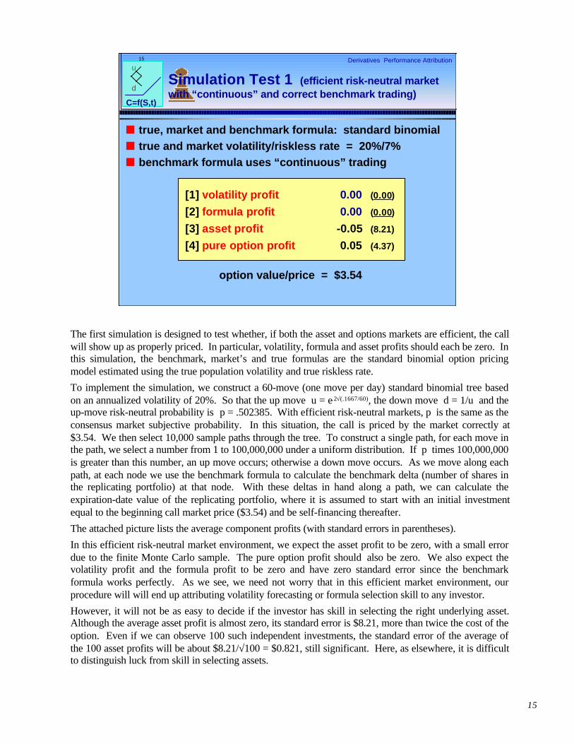
Simulation Test 1 (efficient risk-neutral marketwith “continuous” and correct benchmark trading)

[1] volatility profit 0.00 (0.00)

[2] formula profit 0.00 (0.00)

[3] asset profit -0.05 (8.21)

[4] pure option profit 0.05 (4.37)

option value/price = $3.54

The first simulation is designed to test whether, if both the asset and options markets are efficient, the callwill show up as properly priced. In particular, volatility, formula and asset profits should each be zero. Inthis simulation, the benchmark, market’s and true formulas are the standard binomial option pricingmodel estimated using the true population volatility and true riskless rate.

To implement the simulation, we construct a 60-move (one move per day) standard binomial tree basedon an annualized volatility of 20%. So that the up move u = e.2√(.1667/60), the down move d = 1/u and theup-move risk-neutral probability is p = .502385. With efficient risk-neutral markets, p is the same as theconsensus market subjective probability. In this situation, the call is priced by the market correctly at$3.54. We then select 10,000 sample paths through the tree. To construct a single path, for each move inthe path, we select a number from 1 to 100,000,000 under a uniform distribution. If p times 100,000,000is greater than this number, an up move occurs; otherwise a down move occurs. As we move along eachpath, at each node we use the benchmark formula to calculate the benchmark delta (number of shares inthe replicating portfolio) at that node. With these deltas in hand along a path, we can calculate theexpiration-date value of the replicating portfolio, where it is assumed to start with an initial investmentequal to the beginning call market price ($3.54) and be self-financing thereafter.

The attached picture lists the average component profits (with standard errors in parentheses).

In this efficient risk-neutral market environment, we expect the asset profit to be zero, with a small errordue to the finite Monte Carlo sample. The pure option profit should also be zero. We also expect thevolatility profit and the formula profit to be zero and have zero standard error since the benchmarkformula works perfectly. As we see, we need not worry that in this efficient market environment, ourprocedure will will end up attributing volatility forecasting or formula selection skill to any investor.

However, it will not be as easy to decide if the investor has skill in selecting the right underlying asset.Although the average asset profit is almost zero, its standard error is $8.21, more than twice the cost of theoption. Even if we can observe 100 such independent investments, the standard error of the average ofthe 100 asset profits will be about $8.21/√100 = $0.821, still significant. Here, as elsewhere, it is difficultto distinguish luck from skill in selecting assets.

16


C=f(S,t)

u

d

n true, market and benchmark formula: standard binomialn true and market volatility/riskless rate = 20%/7%

Simulation Test 2 (efficient risk-neutral marketwith “discrete” but correct benchmark trading)

[1] volatility profit -0.005 (0.21) -0.011 (0.28)

[2] formula profit 0.008 (0.15) 0.013 (0.17)

[3] asset profit -0.10 (8.15) 0.08 (8.28)

[4] pure option profit 0.06 (4.14) 0.02 (4.05)


move every 1/2 day move every 1/8 day

n benchmark formula uses “discrete” trading (once a day)

The next simulation checks the robustness of the benchmark replicating strategy to non-continuousobservations. In the previous simulation, it was assumed that every time the underlying asset made abinomial move, the benchmark strategy revised its position based on a freshly calculated delta. This ledto zero volatility sampling error since all paths through a standard binomial tree have the same samplepath volatility.

More realistically, we assume now that we only observe the asset price at “discrete” intervals, that is, aftermore than one binomial move. Moreover, we only calculate the realized volatility based on this sample ofobservations. Since we are not really trading, our reason for this discrete revision is not trading costs, sowe can indeed afford to sample the asset price quite often, perhaps several times intra-day. Nonetheless,it is impractical to sample truly continuously. We also do not want our sample to be significantlyinfluenced by bid-ask bounce; and we also might want to force discrete sampling on our simulation tocrudely capture mild jump risk.

So we revised the simulation by sampling every half day for a total of 120 moves, every quarter day for atotal of 240 moves, and every 1/8 day for a total of 480 moves, in every case covering the 60 days toexpiration. But in each case, we assumed that the benchmark replicating portfolio was revised only at theend of each day and the realized volatility was calculated based only on end-of-day prices. Thecomponent average profits (with standard errors in parentheses) can be found in the attached picture. Thesimulation with a move every 1/4th day shows almost the same standard errors for volatility and formulaprofit as the results of moves every 1/8th day.

In contrast to our earlier simulation, we now have positive standard errors for volatility profit and forformula profit. If we allow ourselves at least a sample of 100 independent option investments, thesestandard errors are quite small (about 1/10th of the errors indicated), so that our techniques are quiterobust to discrete-time benchmark calculations. For example, formula profit is estimated with a standarderror of about two cents.

17


C=f(S,t)

u

dAlternative Risk-NeutralDistributions

0

0.02

0.04

0.06

0.08

0.1

0.12

0.14

-42%

-38%

-34%

-30%

-25%

-21%

-17%

-13% -8

%

-4% 0% 4% 8% 13%

17%

21%

25%

30%

34%

38%

42%

standardized logarithmic returns

prob

abili

ty

NormalSkewed/Kurtic

EdgeworthBinomial Trees

In several of the remaining simulations, the “true formula” is the risk-neutral discounted value of theattached left-skewed and leptokurtic standardized distribution of annualized logarithmic returns. The“normal” distribution describes logarithmic returns which are 60-move standard binomial (with askewness of 0 and a kurtosis of 3). The “skewed/kurtic” distribution describes logarithmic returnsgenerated by an Edgeworth expansion of the 60-move standard binomial with a skewness of -.398 and akurtosis of 4.86.*

This was chosen to match the option-implied distribution from S&P 500 Index options in the years afterthe 1987 stock market crash. In these simulations, the true stochastic process is the unique impliedbinomial tree consistent with this expiration-date distribution following techniques developed inRubinstein (1994).

By contrast, in all but the next simulation, the “market’s formula” is the risk-neutral discounted value ofthe above distribution with a skewness of 0 and kurtosis of 3. This will allow us to examine how theprocedures proposed for performance attribution work when the option market is inefficient in the sensethat it uses the wrong formula (essentially ignoring the left-skewness and leptokurtosis of the trueexpiration-date distribution when it prices options).

*See Rubinstein (1998) for development of techniques to generate unimodal standardized distributions withprespecified third and fourth central moments by transforming a standard binomial distribution via an Edgeworthexpansion.

18


C=f(S,t)

u

d

[1] + [2] mispricing profit 0.001 (0.26)[3] asset profit -0.13 (8.07)[4] pure option profit 0.15 (4.46) value (V) 3.27 (0.26)

payoff (r-tCt) 3.27 (5.01)


Simulation Test 3 (efficient risk-neutral marketwith wrong benchmark formula)

n true and market formula: implied binomial treel skewness = -.398 and kurtosis = 4.86

n true and market volatility/riskless rate = 20%/7%n benchmark formula: standard binomial (“continuous” trading)

For the same level of accuracy, the control variatemethod requires one quarter of one percent of thenumber of observations compared to using r-tCt directly.

Realistically, we do not have the luxury of being able to set our benchmark formula to the one whichactually determines option values and prices. To test the robustness of the benchmark formula to thismisspecification, we continue to assume a risk-neutral efficient market and that the benchmark is thestandard binomial model; but now suppose that the true stochastic process is derived from an impliedbinomial tree where the expiration-date distribution has more leptokurtosis and more left-skewness thanallowed by a standard (constant move size) binomial tree.

In this efficient market, the option mispricing profit is zero. With this now inferior dynamic replicatingstrategy, as expected, the average mispricing profit is virtually zero. Because we are using the wrongbenchmark formula, however, the standard error (compared to our first simulation) is now positive, butnonetheless not large. Again aggregating across 100 independent option investments produces a standarderror of about 3 cents.

We also can directly measure the success of our control variate approach in reducing the standard error inestimating the “true relative value” of the option. The standard error of the payoff r-tCt is $5.01 for asingle option, while the standard deviation of the value V for a single option estimated with the controlvariate is only $0.26, representing about a 95% improvement. To reduce the standard error to about 2.5cents, would require 100 independent observations for V (.26/√100) and 40,000 independentobservations for r- tCt (5.01/√40000). Thus the control variate method requires one quarter of onepercent of the number of observations compared to using r-tCt directly.

For this simulation, we have not reported separate results for volatility and formula profits since thisdecomposition only works properly if the benchmark formula we are using is close to the market’sformula. Since, by assumption for this simulation, these are not the same, this attribution will beincorrect.

19


C=f(S,t)

u

d

market vol = 15% market vol = 25% [1] volatility profit 0.801 (0.00) -0.802 (0.00) [2] formula profit 0.007 (0.32) -0.004 (0.30) [3] asset profit -0.04 (8.12) -0.09 (8.30) [4] pure option profit 0.00 (4.04) 0.11 (4.07)

value (V) 3.55 (0.33) 3.55 (0.29) payoff (r-tCt) 3.48 (5.08) 3.53 (5.19)

option value = $3.54 and option price = $2.74/$4.34

Simulation Test 4 (inefficient risk-neutral optionmarket because market uses wrong volatility)

n true, market and benchmark formula: standard binomialn true and market riskless rate = 7%n true volatility = 20% market volatility = 15%/25%

In the attached simulation results, the market values the option based on an incorrect estimate of volatility.Otherwise, the market makes no mistakes. In particular, it correctly values the asset and uses the trueoption valuation formula. With the true volatility, the option is worth $3.54; but the market errs in onecase by underpricing the option by $0.80, and in another case overpricing the option by $0.80. In thiscase, we would hope that our attribution procedures would calculate an average option mispricing profitof plus or minus 80 cents.

Since we also assume that the benchmark formula is the same as the “market’s formula”, we would alsohope that the procedure would allocate the entire mispricing profit to volatility profit and none of it toformula profit.

As the attached picture shows, we are right on target, with the added plus of low standard errors forvolatility and formula profit.

20


C=f(S,t)

u

dSimulation Test 5 (inefficient risk-neutral optionmarket because market uses wrong formula)

[1] volatility profit -0.000 (0.53)

[2] formula profit -0.284 (0.27)

[3] asset profit -0.24 (7.99)[4] pure option profit 0.00 (4.31) value (V) 3.26 (0.33)

payoff (r -tCt) 3.25 (4.96)

option value = $3.25 and option price = $3.54

n true formula: implied binomial treel skewness = -.398 and kurtosis = 4.86

n true and market volatility/riskless rate = 20%/7%n benchmark and market formula: standard binomial

In the prior simulation, we assumed that the market estimated the volatility incorrectly but got the formularight. In this case, we assume the reverse. Using the standard binomial formula, because the market failsto account for the left-skewness and leptokurtosis of the true underlying stochastic process, it overpricesthe option by about 29 cents.

We would hope that the our procedure would not only capture this overpricing but also attribute itcorrectly all to formula profit and none to volatility profit. Again the attribution procedure comesthrough, with low standard errors to boot.

21


C=f(S,t)

u

dSimulation Test 6 (inefficient risk-neutral optionmarket because market uses wrong volatility/formula)

market vol = 15% market vol = 25% [1] volatility profit 0.793 (0.54) -0.802 (0.53) [2] formula profit -0.282 (0.53) -0.287 (0.36)

[3] asset profit -0.13 (8.03) -0.06 (8.19) [4] pure option profit 0.02 (4.50) 0.06 (4.21)

value (V) 3.25 (0.25) 3.25 (0.54) payoff (r -tCt) 3.25 (4.90) 3.34 (5.10)

option value = $3.25 and option price = $2.74/$4.34


n true and market riskless rate = 7%n true volatility = 20% market volatility =15%/25%n benchmark and market formula: standard binomial

Now we consider simultaneously errors in the market’s estimate of volatility and use of the wrongformula. The market continues to use the standard binomial model, failing to account for non-normalityand in addition under- or over-estimates the volatility. In this case, the option value is $3.25 (as in theprior simulation). We know that the market has made an underpricing error of 29 cents due to use of thewrong formula. In addition, by underestimating (overestimating) the volatility, the market underprices(overprices) the option by an additional 80 cents.

As the attached picture shows, again the attribution procedure works almost perfectly on average with lowstandard errors. Aggregating over 100 independent option investments, the standard errors for volatilityand formula profit are from three to five cents.

22


C=f(S,t)

u

dSimulation Test 7 (inefficient risk-averse marketbecause market uses wrong asset price, volatility, formula)

riskless rate = 5% riskless rate = 9% [1] volatility profit -0.810 (0.54) -0.794 (0.54) [2] formula profit -0.286 (0.24) -0.281 (0.28) [3] asset profit 0.38 (8.03) -0.36 (8.04) [4] pure option profit -0.14 (4.14) 0.20 (4.21)

value (V) 3.09 (0.50) 3.42 (0.58) payoff (r -tCt) 3.29 (4.99) 3.22 (4.89)

option value = $3.25 ($3.07/$3.44) and option price = $4.19/$4.50


n true volatility = 20% market volatility = 25%n true riskless rate = 7% market riskless rate = 5%/9%n benchmark and market formula: standard binomial

This final simulation is like the ending fireworks display on the Fourth of July: we pull out all the stops.To the errors made by the market in the prior simulation, we add potential mispricing of the underlyingasset itself. Alternatively, the simulation can be interpreted as allowing consensus market risk aversion(where before we assumed risk-neutrality).

This modification can be introduced into the simulation quite easily by allowing for the riskless returnavailable in the market to be more or less than the riskless return built into the true stochastic process ofthe underlying asset. We now have two riskless returns. One, the “true” riskless return, is used only todetermine the implied binomial tree describing the actual behavior of the underlying asset. As before, wecontinue to assume this is 7%. So at each node in the implied binomial tree, the up and down move sizesfor the next move are chosen so that the annualized risk-neutral expected return of the underlying assetequals 7%. The market, however, does not understand this. It believes that the riskless return is 5% or9%, and sets the interest rate available to investors accordingly. In particular, this is the interest rate paidon borrowing in the benchmark dynamic replicating strategy. It is also the interest rate used to measurethe various components of performance (since the agency measuring the attribution also doesn’t know anybetter either).

For example, consider the effects of this on asset profit: St - S(r/d)t. In one simulation, the r in thisformula is incorrectly set by the market at 5%. But the asset price actually appreciates at a risk-neutralexpectation of 7%. In a risk-neutral market, we would interpret this as a 2% positive mispricing “alpha”(in which case, the option value is $3.25). In a risk-averse market, we could interpret this ascompensation for bearing risk (in which case, the option value is $3.07). It lies beyond the scope of thispaper to make this distinction. This is the critical issue of asset performance measurement. But undereither interpretation, this should show up as positive asset profit approximately equal to 100(1.07/1.03)1/6

- 100(1.05/1.03)1/6 = 0.32.

So bottom line we hope that our simulation would as in the prior simulation attribute about -80 cents tovolatility profit, and -29 cents to formula profit. Hence, we hope it will show 32 cents asset profit. As theattached picture shows, even with this more complex economy, it continues to sort through the results andattribute the correct volatility and formula profits with low standard errors. In addition, it comesreasonably close on average to capturing the asset profit, although the large standard error makes thisdifficult to rely upon.

23


C=f(S,t)

u

d Summary

Basic attribution: profit due to underlying asset pricechanges vs profit due to option mispricingl robust to discrete trading and wrong benchmark formulal low standard error for option mispricing by using Monte Carlol analysis with dynamic replicating portfolio as control variate

Decompose option mispricing into volatility andformula profitsl requires benchmark formula similar to market’s formulal low standard errors

Unbiased estimate of asset profit in a risk-averse orinefficient asset pricing marketl can not distinguish between risk aversion and inefficiencyl high standard error

V. Summary

We have decomposed the realized profit from an option into two principal components: (1) themispricing of the option at the time of purchase and (2) the profit from subsequent fortuitous changes ormispricing of its underlying asset. We found that the first is relatively easy to isolate, requiring in thesimulations about one-quarter of one percent of the number of observations needed for the second toachieve the same level of accuracy. The trick to this variance reduction is to estimate the “true relativevalue” of the option by using the results of a dynamic replicating strategy as the control variate. Inaddition, this has the further benefit of separating out the profit from mispricing of the underlying asset.The results apply generally irrespective of market risk-aversion.

To separate the mispricing of the option at the time of purchase into volatility and formula profit requiresknowledge of the formula used by the market to price options. But if this formula is known, then thisseparation can be accomplished with few observations.

Although this paper illustrates the attribution approach for a single European call, it can be also be usedfor American options. To apply it to portfolios of derivatives, it will be necessary to consider thecorrelation of their prices to estimate standard errors.

Bibliography

Cox, J.C., S.A. Ross and M. Rubinstein, “Option Pricing: A Simplified Approach,” Journal of FinancialEconomics 7, No. 3 (September 1979), pp. 229-263.

Galai, D., “The Components of the Return from Hedging Options against Stocks,” Journal of Business56, No. 1 (January 1983), pp. 45-54.

Rubinstein, M. “Implied Binomial Trees,” Journal of Finance 49, No. 3 (July 1994), pp. 771-818.

Rubinstein, M. “Edgeworth Binomial Trees,” Journal of Derivatives 5, No. 3 (Spring 1998), pp. 20-27.

derivatives performance attribution 2 derivatives performance attribution c=f(s,t) u d subsequent...

Documents