design, analysis and modelling of computer experiments · scenario : loss of primary coolant ... as...

16/11/2011

Design, analysis and modelling of

computer experiments

Bertrand Iooss

EDF R&D

Cours ECP

2011

ECP - Iooss - 17/11/11 2

Risk quantification areas for EDF

And many uncertainties for the safety due to: • Hazards: demand, hydraulicity, weather patterns, …

• Incomplete knowledge of the systems: ageing, material properties, physics, …

• Internal aggressions: abnormal operating conditions, systems failure, …

• External aggressions: flood, earthquake, storm, …

The assets: • 58 nuclear power plants • 14 thermal power plants • 440 hydro plants & 220 dams • Solar energy and wind power

Goal: • maximize the expect cash flow • minimize the risk Under constraints: customer load, pollution

ECP - Iooss - 17/11/11 3

• Large database of component failures

CLASSICAL STATISTICS

Des avis d’experts

STATISTIQUE BAYESIENNE

Small database of system failures

Expert Judgment

BAYESIAN STATISTICS

• Pas de REX de défaillances

• Un modèle physique

• • No observed failure

• • Physical model

SIMULATION UNCERTAINTY SIMULATION UNCERTAINTY

Research group: component reliability - uncertainty modeling

ECP - Iooss - 17/11/11 4

Uncertainties everywhere in the modeling chain !

Main problem: credibility of predictions

Numerical

model

Input

data

Variables

of interest Algorithm

Physical

model

Physical

phenomenon

Simplifications

Numerical

approximation

Parameters

physicist

Computer scientist

mathematician

statistician

Numerical noise

Model uncertainties

Stochastic uncertainties

Numerical uncertainties

Epsitemic uncertainties

Observations

ECP - Iooss - 17/11/11 5

Example: Simulation of thermal-hydraulic accident

Scenario : Loss of primary coolant accident due to a large break in cold leg

[ De Crecy et al., NED, 2008 ]

Interest output variable Y :

Peak of cladding temperature

p ~ 10-50 input random variables X:

geometry, material properties, environmental conditions, …

Goal: safety criterion

Computer code Y =f (X)

Time cost ~ 1-10 h - n ~ 100 - 500

Pressurized water nuclear reactor

Source: CEA

ECP - Iooss - 17/11/11 6

Similar safety and uncertainty issues in CS&E and Nature

sciences

Climate Modeling :

Prediction

Car and

plane:

Conception

Nuclear industry :

Conception,

Maintenance, risks

Oil, gas, CO2:

Production optimization

CS&E : Computational Science & Engineering

Astrophysics:

Understanding

ECP - Iooss - 17/11/11 7

• Modeling phase:

– Improve the model

– Explore the best as possible different input combinations – Identify the predominant inputs and phenomena in order to priorize R&D

• Validation phase:

– Reduce prediction uncertainties

– Calibrate the model parameters

• Practical use of a model:

– Safety studies: assess a risk of failure (rare events)

– Conception studies: optimize system performances and robustness

Main stakes of uncertainty management

ECP - Iooss - 17/11/11 8

Uncertainties in simulation experiments 2211 xaxaY

2211 xaxaY

Ancient way

X1

X2

1x

2x

Still learned in Schools

2

2

2

2

2

1

2

1 aaY

Pre-modern way

x's identified to R.V. … but same algebra

Still used in metrology (GUM)

Really Modern way

x's fully treated as R.V.

Can give moments, quantiles, and even pdf of Y … …if fair waiting time

X1

X2

DoE

X2

X1

Sampling

ECP - Iooss - 17/11/11 9

Uncertainty management - The generic methodology

ECP - Iooss - 17/11/11 10

Which criteria?

The uncertain inputs are modeled thanks to a random vector X, composed

of p univariate random variables (X1, X2, …, Xp) linked by a dependence

structure => is a random variable

• Different quantities of interest on Z

– These different objectives are embodied by different criteria upon the

output variable of interest.

• These criteria can focus on:

– its range : we only want to evaluate its min and maximum possible

values. For example, in the prior stage of the design of a new concept.

– its central dispersion : we want to evaluate its expected values and its

dispersion around it. For example, in the design stage of a product.

– its probability of exceeding a threshold : usually, the threshold is

extreme. For example, in the certification stage of a product.

• Formally, the quantity of interest is a particular feature of the pdf of the

variable of interest Z

ECP - Iooss - 17/11/11 11

Why these questions are so important?

• The proper identification of:

– the uncertain input parameters and the nature of their

uncertainty sources,

– the output variable of interest and the goals of a given

uncertainty assessment,

• is the key step in the uncertainty study, as it guides the choice of the

most relevant mathematical methods to be applied

What is really relevant in the uncertainty study?

m

Mean, median, variance,

(moments) of Z

Pf

threshold

(Extreme) quantiles, probability

of exceeding a given threshold

ECP - Iooss - 17/11/11 12

A particular quantity of interest: the “probability of failure”

• G models a system (or a part of it) in operating conditions – Variable of interest Z a given state variable of the system (e.g. a temperature, a

deformation, a water level etc.)

• Following an « operator » point of view – The system is in safe operating condition if Z is above (or below) a given “safety” threshold

• System “failure” event: – Classical formulation (no loss of generality) in which the threshold is 0 and the system fails

when Z is negative

– Structural Reliability Analysis (SRA) “vision”: Failure if C-L < 0 (Capacity – Load)

• Failure domain:

• Problem: estimating the mean of the random

variable “failure indicator”:

ECP - Iooss - 17/11/11 13

Outline

1.Design of numerical experiments – Space filling designs

2. Analysis of numerical experiments

3. Modelling of numerical experiments

4. Application

ECP - Iooss - 17/11/11 14

Typical engineering practice : One-At-a-Time (OAT) design

Main remarks :

OAT brings some information, but potentially wrong

Exploration is poor : Non monotonicity ? Discontinuity ? Interaction ?

X1

X2

P1

P2 P3

ECP - Iooss - 17/11/11 15

Model exploration – Example: Flood model

Inputs

Q = river flowrate [500,3000]

Ks = friction coefficient [15,50]

Zv = downstream river bed heigth [49,51]

Zm = upstream river bed heigth (=55 m)

Hd = dyke heigth [7,9]

Cb = bank heigth [55,56]

L = river length (=5000m)

B = river width (=300m)

Simplified physical model (hydraulics)

dyke

S = overflowing heigth

Cp = annual cost of dyke maintenance

ECP - Iooss - 17/11/11 16

Typical engineering practice : One-At-a-Time (OAT) design

Q [500,3000] ; Ks [15,50] ; Zv [49,51] ; Hd [7,9] ; Cb [55,56]

Computation with maximal inputs : S = -10.77 ; Cp = 0.71

Computation with minimal inputs : S = -10.99 ; Cp = 0.65

Adding some physical knowledge about the simulated phenomenon

Computation giving maximal output (Ks,Hd,Cb down; Q,Zv up): S = -4.34 ; Cp = 1.35

Computation giving minimal output (Ks,Hd,Cb up; Q,Zv down): S = -15.02 ; Cp = 0.67

(Ks,Cb up; Q,Zv,Hd down): Cp = 0.63 (not the global minimum)

With a single input variation from max Q Ks Zv Hd Cb

S -8.73 -7.77 -7.10 -6.34 -5.34

Cp 0.73 0.79 0.86 1.02 1.17

Conclusions : OAT brings some information, but potentially wrong

Exploration is poor : Non monotonicity ? Discontinuity ? Interaction ?

ECP - Iooss - 17/11/11 17

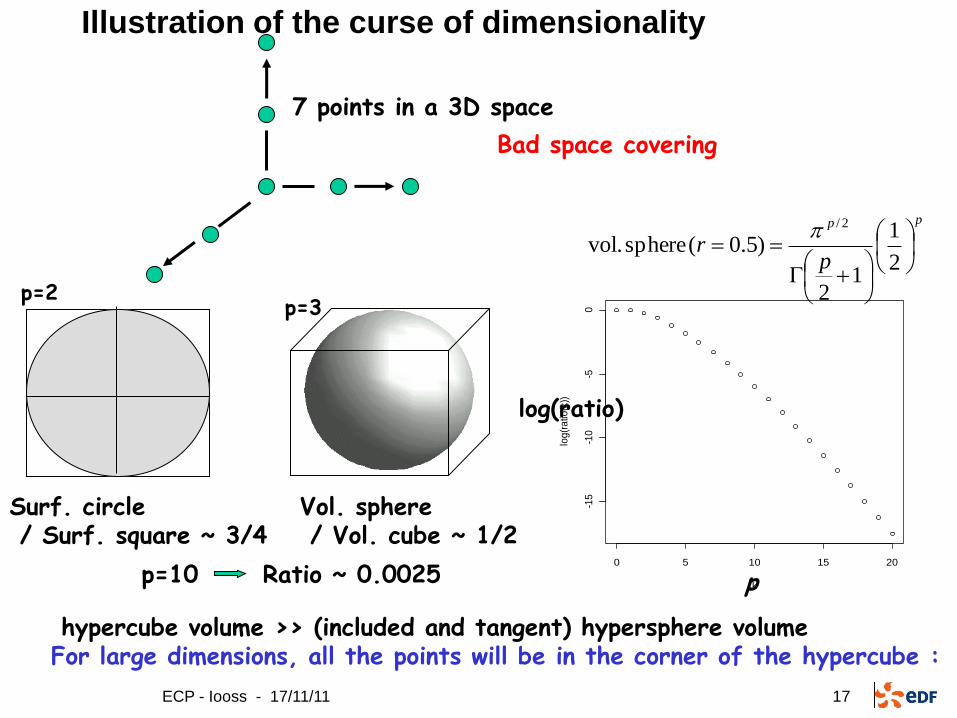
Illustration of the curse of dimensionality

7 points in a 3D space

p=2 p=3

Surf. circle / Surf. square ~ 3/4

Vol. sphere / Vol. cube ~ 1/2

p=10 Ratio ~ 0.0025 0 5 10 15 20

-15

-10

-50

k

log

(ra

tio(k

))

Bad space covering

p

log(ratio)

hypercube volume >> (included and tangent) hypersphere volume For large dimensions, all the points will be in the corner of the hypercube :

pp

pr

2

1

12

)5.0( sphere vol.2/

ECP - Iooss - 17/11/11 18

Model exploration goal

GOAL : explore as best as possible the behaviour of the code

Put some points in the whole input space in order to « maximize » the amount of information on the model output

Contrary to an uncertainty propagation step, it depends on p

Regular mesh with n levels N =n p simulations

To minimize N, needs to have some techniques ensuring good « coverage » of the input space

Simple random sampling (Monte Carlo) does not ensure this

Monte Carlo Optimized design

Ex: p = 2 N = 10

Ex: p =2, n =3

N =9

p = 10, n=3

N = 59049

ECP - Iooss - 17/11/11 19

Objectives

When the objectives is to discover what happens inside the model and when no model computations have been realized, we want to respect the two following constraints:

• To spread the points over the input space in order to capture non linearities of the model output,

• To ensure that this input space coverage is robust with respect to dimension reduction.

Therefore, we look some design which insures the « best coverage » of the input space

• How to define this « best » ?

• How to choose the right number of points ?

• How to measure the representativity ?

ECP - Iooss - 17/11/11 20

The design of numerical experiments: 1) Space filling

Sparsity of the space of the input variables in high dimension The learning design choice is made in order to have an optimal coverage

of the input domain The space filling designs are good candidates. Example: Sobol sequence Two possible criteria:

1. Distance criteria between the points: minimax, maximin, … 2. Uniformity criteria of the design (discrepancy measures)

Simple Random Sample(SRS)

Space Filling Design (SFD)

ECP - Iooss - 17/11/11 21

Distance criteria between the points

• Minimax design DMI : Minimize the maximal distance between the points

All points in [0,1]p are not too far from a design point

=> One of the best design

but too expensive to find DMI

• Maximin design DMA : Maximize the minimal distance between the points

),(min),( re whe

),(max),(maxmin

)0(

)0(xxdDxd

DxdDxd

Dx

MIxxD

[ Johnson et al., 1990 ] [ From: Owen, 1996 ]

),(min),(minmax )2()1(

,

)2()1(

, )2()1()2()1(xxdxxd

MADxxDxxD

ECP - Iooss - 17/11/11 22

Space filling measure of a design: the discrepancy

Measure of the maximal deviation between the distribution of the sample’s points to an uniform distribution

Measure of deviation from the uniformity Geometrical interpretation: Comparison between the volume of intervals and the number points within these intervals

Lower the discrepancy is, the more the points of

the design D fill the all space

p

i

i

tQ

tQ

p

p

tN

ND

ttttQtQ

p1

)(

[1,0[)(

21

sup)(disc

[,0[[,0[[,0[)(,[1,0[)(

ECP - Iooss - 17/11/11 23

Discrepancy computation in practice

• Modified L2-discrepancy (intervals with minimal boundary 0)

• Centered L2-discrepancy (intervals with boundary one vertex of the unit cube)

• Symetric L2-discrepancy (intervals with boundary one « even » vertex of the unit cube)

Different definitions, depending on the chosen norm & considered intervals

Classical choice (easy computations): L2 – discrepancy

N

ji

p

k

j

k

i

k

j

k

i

k

N

i

p

k

i

k

i

k

p

xxxxN

xxN

D

1, 1

)()()()(

2

1 1

2

)()(

2

2

1

2

1

2

1

2

1

2

11

1

2

1

2

1

2

1

2

11

2

12

13)(disc

ECP - Iooss - 17/11/11 24

Relation with the integration problem

NO

N

NIII

x

xfN

I

dxxfI

NN

p

Ni

i

N

i

i

N

p

1)(VarVar;

[1,0[in points random of sequence a with

)(1

: Carlo Monte

)(

MCMC

...1

)(

1

)(MC

[1,0[

General property: With a low discrepancy sequence D (quasi Monte Carlo sequence) : Well-known choice: Sobol’ sequence

N

NO

pln

)(disc)( DfV

ECP - Iooss - 17/11/11 25

Sobol’sequence vs. Random sample vs. regular grid

[ From: Kucherenko, 2010 ]

ECP - Iooss - 17/11/11 26

The design of numerical experiments: 2) LHS

A lot of models are additive. If not, first order effects often dominate

Property of uniform projections on the margins

It can be obtained via a Latin Hypercube Sample

Divide each dimension in N intervals

Take one point in each stratum

Example : p =2, N =10, X1 ~ U[0,1], X2 ~ N(0,1)

Example : p =2, N =4

ECP - Iooss - 17/11/11 27

Algorithm of LHS – Stein method

Sample with N points of p inputs

ran = matrix(runif(N*p),nrow=N,ncol=p)

# tirage de N x p valeurs selon loi U[0,1]

for (i in 1:p)

{

idx = sample(1:N) # vecteur de permutations des entiers {1,2,…,N}

P = (idx-ran[,i]) / N # vecteur de probabilites

x[,i] <- quantile_selon_la_loi (P)

}

ECP - Iooss - 17/11/11 28

Optimization of LHS

Joining the two properties (space filling and LHS) One possibility: generate a large number (for ex: 1000) of different LHS Then, choose the LHS which optimizes the criterion Maximin LHS Low wrap-around For comparison: discrepancy LHS Sobol sequence

0.2 0.4 0.6 0.8

0.2

0.4

0.6

0.8

x[,1]

x[,2

]

Example: p = 2 – N = 16

ECP - Iooss - 17/11/11 29

Important property: robustness in terms of subprojections

Most of the times, the function f (X) has low effective dimensions: - in the truncation sense (p1 = number of influent inputs) p1 << p - in the superposition sense (p2 = higher order of influent interaction) p2 << p

Then, we need SFD which keeps their space-filling properties in low-dimensional

subspaces (by importance: in dimensions p ’=1, then p ’=2, ...)

good bad

• p ’ = 1 LHS ensures good 1D projection properties

• p ’ 2 In their definition, some L2-discrepancy criteria take into account subprojections In contrary design points distance criteria are not robust at all

ECP - Iooss - 17/11/11 30

Outline

1.Design of numerical experiments

2. Analysis of numerical experiments – Sensitivity analysis

3. Modelling of numerical experiments

4. Application

ECP - Iooss - 17/11/11 31

Sensitivity analysis notions

• Sensitivity, for example

Donne une idée de la manière dont peut répondre la réponse en fonction de variations potentielles des facteurs

• Contribution = sensitivity x importance, for example

Permet de déterminer le poids d’une variable d’entrée (ou groupe de variables) sur l’incertitude de la variable d’intérêt (la sortie)

iXY

)( i

i

XX

Y

DX DY

f

X Y

ECP - Iooss - 17/11/11 32

Main objectives of sensitivity analysis

• Reduction of the uncertainty of the model outputs by prioritization of the sources

• Variables to be fixed in order to obtain the largest reduction (or a fixed reduction) of the output uncertainty

A purely mathematical variable ordering

• Most influent variables in a given output domain

if reducibles, then R&D prioritization

else, modification of the system

• Simplification of a model

• determination of the non-influent variables, that can be fixed without consequences on the output uncertainty

• building a simplified model, a metamodel

ECP - Iooss - 17/11/11 33

(quantity of interest = variability of the output)

Three types of answers: 1. Screening :

- classical design of experiments, - numerical design of experiments (Morris, sequential bifurcation)

2. Quantitative measures of global influence : - correlation/regression on values/ranks - statistical tests, - functional variance decomposition (Sobol), - other measures : entropy, distribution distances

3. Deep exploration of sensitivities - smoothing techniques (param./non parametric) - metamodels

Overall classification of sensitivity analysis methods

X1

X3

X2

Y

ECP - Iooss - 17/11/11 34

X1

X2

Screening without hypothesis on function: Morris’ method

• Discretization of input space

• computation of one elementary effect for each input

P1

• Needs p+1 experiments • OAT (One-at-A-Time)

P2 P3

ECP - Iooss - 17/11/11 35

X1

X2

1

5

4

3

2

• OAT design is repeated R times (total: n = R*(p+1) experiments) • It gives an R-sample for each elementary effect

• Sensitivity measures:

Morris’ method

ECP - Iooss - 17/11/11 36

Morris: sensitivity measures

• is a measure of the sensitivity:

Important value important effects (in mean) sensitive model to input variations

• is a measure of the interactions and of the non linear effects:

important value different effects in the R-sample effects which depend on the value:

• of the input Xi => non linear effect • or of the other inputs => interaction (the distinction between the two cases is impossible)

ECP - Iooss - 17/11/11 37

Morris : example

*m

Cas test : non monotonic function of Morris

20 factors 210 simulations Graph (mu*, sigma)

Distinction between 3 groups:

1. Negligible effects 2. Linear effects 3. Non linear effects

and/or with interactions

1

3

2

ECP - Iooss - 17/11/11 38

Example : fuel irradiation computation in HTR

Code de calcul ATLAS (CEA) : simulation du comportement du combustible à particules sous irradiation Noyau de matière fissile Carbone pyrolytique poreux Carbone pyrolytique dense Carbure de Silicium Sources de contamination : rupture de particules Etudes de fiabilité

La rupture d’une particule peut être provoquée par la rupture des couches denses externes (IPyC, SiC, OPyC) Les réponses sont choisies pour être représentatives du phénomène de rupture : contraintes orthoradiales maximales dans les couches externes

Nombre de particules dans un réacteur : de 109 à 1010

!

< 1mm

ECP - Iooss - 17/11/11 39

3 uncertainty types in inputs • 10 paramètres de fabrication des particules (épaisseurs, …) Spécifications de fabrication lois normales tronquées • 5 paramètres d’irradiation (température, …)

Intervalle [min,max] lois uniformes

• 28 lois de comportement (fonctions des température, flux, …) Avis d’expert constantes multiplicatives (de loi U[0.95,1.05])

Exemple : loi de densification

du PyC

ECP - Iooss - 17/11/11 40

Results of Morris

Grande sensibilité à ces entrées (épaisseurs, température d’irradiation) Interactions faibles

Les lois sur le fluage et la densification du PyC sont les lois auxquelles le code est le plus sensible

Conclusion : La méthode de Morris donne une idée de la manière dont peut répondre la sortie en fonction de variations potentielles des entrées… Utile pour identifier les entrées potentiellement influentes

p = 43 entrées, 20 répétitions, n = 860 calculs, coût unitaire ~ 1 mn 14h

ECP - Iooss - 17/11/11 41

(quantity of interest = variability of the output)

Three types of answers: 1. Screening :

- classical design of experiments, - numerical design of experiments (Morris, sequential bifurcation)

2. Quantitative measures of global influence : - correlation/regression on values/ranks - statistical tests, - functional variance decomposition (Sobol), - other measures : entropy, distribution distances

3. Deep exploration of sensitivities - smoothing techniques (param./non parametric) - metamodels

Overall classification of sensitivity analysis methods

X1

X3

X2

Y

ECP - Iooss - 17/11/11 42

Sensitivity analysis for one scalar output

Sample ( Xp, Y (X ) ) of size N > p

Preliminary step: graphical vizualisation (for ex: scatterplots) Remark: it can be a Monte Carlo sample, a quasi-Monte Carlo sample or any other designs

ECP - Iooss - 17/11/11 43

Flood model - Scatterplots – Output S

Monte Carlo sample – N = 100

ECP - Iooss - 17/11/11 44

Flood model - Scatterplots – Output Cp


Major drawback: only first order relations between inputs are analyzed and not their interactions (=> needs of other data anlysis tools)

ECP - Iooss - 17/11/11 45



? Linear relation ?

Oui

Linear

regression

between Xi

and Y

Regression

coefficients

(R²)

Sensitivity indices Sobol’ indices

Non ? Monotonic relation ?

Oui Non

Regression on

ranks

(R²*)

Preliminary step: graphical vizualisation (for ex: scatterplots) Quantitative sensitivity analysis methodology [Saltelli et al. 00, Helton et al. 06 ]

ECP - Iooss - 17/11/11 46

Sensitivity indices in case of linear inputs/output relation

Independent input variables

Sample : n realizations of

• SRC index:

Sign of bi gives the direction of variation of Y in fct of Xi

• SRC is similar to the linear correlation coefficient (Pearson)

• Validity of the linear model via

The residuals diagnostics and R² :

• We have => nice interpretation of SRC

46

p

i

ii XY1

0 bb

)Var(

)Var(:

Y

XXSRC i

ii b

Y,X

n

i

i

n

i

ii

YY

YY

R

1

2

1

2

2

ˆ

1

pX,X ...,1X

p

i

iXR1

22 SRC

ECP - Iooss - 17/11/11 47

Flood model - Output S


31% 15% 18% 29% 6%

Sensitivity indices (SRC2)

The model is linear (R²=0.99)

SRC coefficients are sufficient for the quantitative sensivity analysis

ECP - Iooss - 17/11/11 48



? Linear relation ?

Oui

Linear

regression

between Xi

and Y

Regression

coefficients

(R²)

Sensitivity indices Sobol’ indices

Non ? Monotonic relation ?

Oui Non

Regression on

ranks

(R²*)

Preliminary step: graphical vizualisation (for ex: scatterplots) Quantitative sensitivity analysis methodology [Saltelli et al. 00, Helton et al. 06 ]

)Var(

)]Var[E(

Y

XYS

i

i

ECP - Iooss - 17/11/11 49

Properties ( xi ~ U[O,1] for i=1,…,p , the xi s are independent)

Example :

pLf ]1;0[)()( 2 xxx

pp

i ij

jiij

p

i

ii xxxfxxfxfffy ,...,,...,)( 21,...,2,1

1

0

x

with

Functional decomposition

Infinity of possible decompositions

BUT, unicity of decomposition if:

)E(0 ydff xx

00 )|E()( fxyfdxfxf iiii x

0)|E()|E(),|E(, fxyxyxxyxxf jijijiij

0),(;2

1)(;

2

1)(;1

]1;0[~;]1;0[~;),(

21122221110

212121

xxfxxfxxff

UxUxxxxxf

sjiiii iijdxxxfss

,...,0),...,( 1... 11

ECP - Iooss - 17/11/11 50

Sensitivity indices without model hypotheses

Sobol indices definition:

• First order sensitivity indices:

• Second order sensitivity indices:

• ...

50

)Var(Y

VS i

i

)Var(Y

VS

ij

ij

)()()()(Var 12

1

YVYVYVY p

p

ji

ij

p

i

i <

Functional ANOVA [Efron & Stein 81] (hyp. of independent Xi s) :

... , )E(Var

)]E([Var)( where

jijiij

ii

VVXXYV

XYYV

ECP - Iooss - 17/11/11 51

Graphical interpretation

2 4 6 8 10 12 14

02

46

810

per1

p23

0 20 40 60 80

02

46

810

kd1

p23

0 50 100 150

02

46

810

kd2

p23

0.00 0.02 0.04 0.06 0.08 0.10

02

46

810

i3

p23

First order Sobol’ indices measure the variability of consitional expectation des espérances (mean trend curves in the scatterplots)

Null index

Small index

High index

ECP - Iooss - 17/11/11 52

1i

iS

1i

iS

Always

Additive model

i

iS1 Measure the degree of interactions between variables

k

i j k

ijk

i j

ij

p

i

i SSSS ,...,2,1

1

...1

Sobol’ indices properties

Examples : p =4 gives 4 indices Si, 6 indices Sij , 4 indices Sijk, 1 indice Sijkl General case : 2p-1 indices to be estimated Total sensitivity index: [ Homma & Saltelli 1996 ]

i

j kj

ijkijiTi SSSSS ~

,

1...

ECP - Iooss - 17/11/11 53

Direct estimation via Monte Carlo

2 i.i.d. samples :

Variance (classical estimator) :

Conditional variances :

• Quasi Monte Carlo

• FAST

• …

n

k

kn

k

k fn

fffn

YV1

)(

0

1

2

0

2)( 1ˆ avec ˆ1)(ˆ XX

2

0

)()(

1

)()(

1

)(

1

)()(

1

)()(

1

)(

1

1

22

',...,',,',...,',...,,,,...,1

)(ˆ

EE)]Var[E()(

fXXXXXfXXXXXfn

YV

dXXYdXXYXYYV

k

p

k

i

k

i

k

i

kk

p

k

i

k

i

k

i

kn

k

i

iiiiii

njpi

j

injpi

j

i XX,..,1;,..,1

)(

,..,1;,..,1

)( 'et

2

0

)()(

1

)()(

1

)(

1

)()(

1

)()(

1

)(

1

1

~

~~

,...,,',,...,,...,,,,...,1

)(ˆ

)]Var[E()(

fXXXXXfXXXXXfn

YV

XYYV

k

p

k

i

k

i

k

i

kk

p

k

i

k

i

k

i

kn

k

i

ii

ECP - Iooss - 17/11/11 54

Flood model

ECP - Iooss - 17/11/11 55

The sampling-based approaches


? Linear relation ?

Yes

Linear

regression

between X

and Y

Regression

coefficients

(R²)

Sensitivity indices

Sobol indices

No ? Monotonic relation ?

Yes No

Regression on

ranks

(R²*)

large

negligible

Smoothing

Metamodel

N > 10 p

Monte Carlo

N > 1000 p

? CPU time cost

of the model ?

Quasi-MC,

FAST, RBD,

N > 100 p

small

ECP - Iooss - 17/11/11 56

Flood model – Output Cp

From the 100-size Monte Carlo sample, a Gaussian process metamodel is fitted

Predictivity of the Gp metamodel : Q2 = 99%

N=1e5

100 replicates

N x (p+2) x 100 = 7e7 evaluations

ECP - Iooss - 17/11/11 57

Classification of sensitivity analysis methods

p 10p 1000p

Linear 1st

degree

Monotonic + interactions

Monotonic without

interaction

Metamodel

2p

Morris

( p = number of input variables )

0

Non monotonic

Number of model f

evaluations

Super screening

Variance decomposition

Design of experiment

Rank regression

Linear regression

Complexity/regularity of model f

Calculations of all types of indices (Sobol, distribution-based, …)

+ main effects E(Y | Xi )

Screening

Sobol indices

Monte-Carlo sampling

design, analysis and modelling of computer experiments · scenario : loss of primary coolant ... as...

Documents