design and implementation of pattern recognition algorithms …monica/research/publications/... ·...
TRANSCRIPT

University of Nevada, Reno
Design and Implementation of Pattern Recognition Algorithms for the Detection of Chemicals with a Microcantilever Sensor Array
A thesis submitted in partial fulfillment of the requirements for the degree of Master of Science in
Computer Science
by
Asya F. Nikitina
Dr. Monica Nicolescu/Thesis Advisor
December, 2007

© by Asya F. Nikitina 2007 All Rights Reserved

We recommend that the thesis prepared under our supervision by
ASYA F. NIKITINA
entitled
Design and Implementation of Pattern Recognition Algorithms for the Detection of Chemicals with a Microcantilever Sensor Array
be accepted in partial fulfillment of the
requirements for the degree of
MASTER OF SCIENCE
Monica Nicolescu, Ph.D., Advisor
Mircea Nicolescu, Ph.D., Committee Member
Joseph I. Cline, Ph.D., Graduate School Representative
Marsha H. Read, Ph. D., Associate Dean, Graduate School
December, 2007
THE GRADUATE SCHOOL

i
Abstract
Nowadays, we are witnesses to the noticeable success in the development of a
new class of chemical and biological sensors – microfabricated cantilever sensor arrays
actuated at their resonance frequencies and functionalized by polymer coatings. The
major advantages of such miniature sensors are their small size, fast response, remarkably
high sensitivity, and the endless possibilities of reaching high selectivity via customized
combination of polymer coatings. These devices are inexpensive, portable, and have the
ability to operate in various environments, such as vacuum, air and liquids. The areas of
applications of microfabricated cantilever sensor arrays are almost countless, including a
variety of scientific research in physics, chemistry, biochemistry, biology, and genetics,
food and beverage industry, perfume industry, pharmacology, medicine, environmental
monitoring, and most recently, related to the national security due to a high risk of
terrorist attacks.
However, despite the remarkable achievements in fabrication of microcantilever
sensor arrays, creating an accurate and reliable pattern recognition algorithm as a part of
the sensory system is still an essential and not yet completely solved problem. Most
pattern analysis algorithms that have been used with the cantilever sensor arrays today
are highly customized, ad hoc algorithms. They often lack generality and cannot be easily
carried from one set of experimental data to another. Therefore, the main goal of the
current work was developing a pattern recognition algorithm that can be highly effective
on a given set of sensory data and easily adjustable to any new set of data.

ii
Acknowledgments
I would like to take this opportunity to express my most sincere gratitude to my
research advisor at the University of Nevada, Reno, Dr. Monica Nicolescu for giving me
the opportunity to work in her research group, for her guidance, constant support, and
help.
I greatly thank Dr. Joseph Cline for helping me with my research project and
Dr. Mircea Nicolescu for helping me with my thesis. I also thank both Dr. Joseph Cline
and Dr. Mircea Nicolescu for spending their valuable time to read my thesis.
Thanks to Dr. Carl Looney for exposing me to fuzzy systems and neural
networks. I also thank Dr. Jesse Adams and Ben Rogers from Nevada Nanotech System,
Inc. for giving me the opportunity to work in their lab and for their help with the
experimental part of the project.
Thanks to our research group members: Chris King, Sebastian Smith, and Austin
Stanhope for their help. Also thanks to Jihyo Chong for helping me to collect the
experimental data.
Financial support by an NSF-EPSCoR Sensors fellowship is greatly
acknowledged.

iii
1 Introduction ......................................................................................................................... 1
2 Related Work ...................................................................................................................... 6
3 Experimental Setup ........................................................................................................... 14
3.1 Experimental Setup ....................................................................................................... 14
3.2 Experiment Protocol Description .................................................................................. 18
3.3 Data Collection Results ................................................................................................. 22
3.4 Feature Extraction ......................................................................................................... 26
4 Theory and Algorithms Details ......................................................................................... 31
4.1 Extended Classifier System (XCS) ............................................................................... 33
4.2 Kernel-Based Pattern Recognition Methods ................................................................. 51
5 Experimental Results ........................................................................................................ 88
5.1 Extended Classifier System (XCS) ............................................................................... 91
5.2 Radial Basis Function Neural Network (RBF NN) ...................................................... 92
5.3 Support Vector Machines (SVMs) ................................................................................ 93
5.4 Fuzzy Neural Network (FNN) ...................................................................................... 96
5.5 Fuzzy Classifier based on Fuzzy C-Means Clustering (FCM-based) ........................... 98
5.6 Fuzzy Classifier based on Fuzzy Connectivity Clustering (FCC-based) .................... 100
6 Conclusion and Future Work .......................................................................................... 103
7 Appendices ...................................................................................................................... 108
7.1 Appendix A – Implementation Details of XCS Algorithm ........................................ 108
7.2 Appendix B – Implementation Details of FCC Algorithm ......................................... 111
8 References ....................................................................................................................... 112

iv
Table 1. Results of classification accuracy obtained by using the constant exploration rate
……………………………...……………………………………………………………47
Table 2. Adjusting gradient exploration rate scheme ...…………………………..……..….47
Table 3. Results of classification accuracy obtained for different niche mutation rates……49
Table 4. Results for classification accuracy with and without action mutation ……………49
Table 5. Results of classification accuracy for different deletion schemes …………..........50
Table 6. The results of classification accuracy of RBF NN algorithm on the Wisconsin data
set using 7-fold cross validation ………………………………………………...……....57
Table 7. The results of classification accuracy of SVM algorithm on the Wisconsin data set
using 7-fold cross validation …………………………………………………………....61
Table 8. The results of classification accuracy of FNN algorithm on the Wisconsin data set
using 7-fold cross validation .……………………………………………...…................66
Table 9. The results of classification accuracy of FCM-based algorithm on the Wisconsin
data set using 7-fold cross validation ………………………………………..………….80
Table 10. The results of classification accuracy of FCC-based algorithm on the Wisconsin
data set using 7-fold cross validation …………………………...……….……………...86
Table 11. Class labels according to the presence of the specified concentration of different
chemical vapors in the analyzed gaseous mixture and the number of feature vectors in
each class …………………………………..…………….……………………………...88
Table 12. Information about training/testing set pairs for algorithm's accuracy evaluation..90
Table 13. The results of classification accuracy of the XCS algorithm using the cantilever
sensor array data ………………………………………………………………….……..91

v
Table 14. The results of classification accuracy of the RBF NN algorithm using the
cantilever sensor array data ………………………………………………………….…..93
Table 15. The results of classification accuracy of the SVM algorithm with the Gaussian
kernel using the cantilever sensor array data ………………………………………..…..94
Table 16. The results of classification accuracy of the SVM algorithm with the linear kernel
using the cantilever sensor array data …………………………………………………...95
Table 17. The results of classification accuracy of the SVM algorithm with the polynomial
of degree 3 kernel using the cantilever sensor array data …………..….………………..96
Table 18. The results of classification accuracy of the FNN algorithm with the discriminant
function f 1 using the cantilever sensor array data ………….……….…………………..97
Table 19. The results of classification accuracy of the FNN algorithm with the discriminant
function f 2 using the cantilever sensor array data ……..……………………………..…98
Table 20. The results of classification accuracy of the fuzzy classifier based on FCM-based
algorithm with the discriminant function f 1 using the cantilever sensor array data …....99
Table 21. The results of classification accuracy of the fuzzy classifier based on FCM-based
algorithm with the discriminant function f 2 using the cantilever sensor array data …..100
Table 22. The results of classification accuracy of the semi-supervised version of the FCC-
based algorithm using the cantilever sensor array data .……..……...………………....101
Table 23. The results of classification accuracy of the full version of the FCC-based
algorithm that clustered labeled vectors separately from unlabeled ones using the
cantilever sensor array data …………………………………….……………...…….....102

vi
Table 24. A list of important parameters and their values used in the current implementation
……………………………………………………………...…………………………...109

vii
Figure 1. Basic experimental setup. ........................................................................................ 14
Figure 2. Flow rate control system for controlling the desired concentration of the chemical
vapors. ............................................................................................................................... 15
Figure 3. Temperature adjustment box for controlling the temperature of the array cell. ...... 16
Figure 4. The location of the M10 cantilever array within the system. .................................. 16
Figure 5. The figure shows a snapshot of all ten resonance frequencies. ............................... 18
Figure 6. Temperature calibration curve (all cantilevers on the same graph). ....................... 20
Figure 7. Resonance frequency shifts of all cantilevers during exposure of the array to 18%
of acetone. ......................................................................................................................... 23
Figure 8. Heights of resonance frequency peaks of all cantilevers during exposure of the
array to 18% of acetone. ................................................................................................... 23
Figure 9. Resonance frequency shifts of all cantilevers during exposure of the array to 7% of
ethanol. .............................................................................................................................. 24
Figure 10. Heights of resonance frequency peaks of all cantilevers during exposure of the
array to 7% of ethanol. ...................................................................................................... 24
Figure 11. Resonance frequency shifts of all cantilevers during exposure of the array to 26%
of toluene. ......................................................................................................................... 25
Figure 12. Heights of resonance frequency peaks of all cantilevers during exposure of the
array to 26% of toluene. .................................................................................................... 25
Figure 13. The figure shows the measurements for resonance frequency of the cantilever
coated with OV275 polymer. ............................................................................................ 27

viii
Figure 14. The figure shows the measurements for resonance frequency of the cantilever
coated with BSP3 polymer. ............................................................................................... 28
Figure 15. The figure shows the measurements for resonance frequency of the cantilever
coated with PBM polymer. ............................................................................................... 29
Figure 16. Schematic illustration of XCS's performance cycle. ............................................. 36
Figure 17. New flexible scheme for action selection that can be finely adjusted to each
specific problem space. ..................................................................................................... 38
Figure 18. The classifier’s accuracy as a function of the classifier prediction error εj. .......... 40
Figure 19. The radial basis function neural network (RBF NN) architecture. ....................... 54
Figure 20. Separating hyperplane, margins, and support vectors. .......................................... 60
Figure 21. Representation of a fuzzy classifier as a fuzzy neural network. ............................ 63
Figure 22. Class diagram of the OOP implementation of the FCC algorithms. ................... 111

1
1 Introduction
There always has been a high interest in developing micromechanical devices for
analyte detection for various applications such as quality and process control in industry,
disposal diagnostics for biomedical analyses, pharmacological screening, gas sensing
devices for environmental and health-related agencies, forensic investigations, fragrance
design, and many others. Recently, the new threat of international terrorism brought the
urgency for developing such sensor devices to a new high level. The new demand
brought new requirements: now not only should sensors be highly sensitive to a wide
range of target analytes, but they should also be miniaturized, automated, cost effective,
reliable and robust.
The concept of chemical and biochemical sensors has been a subject of extensive
research efforts for a long time. The conventional approach to chemical sensors
traditionally uses an approach called “lock-and-key” design, where a specific receptor is
synthesized for each analyte of interest. This type of sensors is extremely selective, but
usually quite expensive and has limited potential to meet today’s real-life demand for
detection of a broad range of analytes with the same sensor device.
A new revolutionary approach to chemical and biochemical sensors is closer
conceptually to our own sense of olfaction. In this approach, instead of the strict “lock-
and-key” single sensor design architecture, an array of different sensors, each of which
responds to different chemicals or even different classes of chemicals is used [1], [2], [3].
The idea behind this design is that the sensors of this array should contain as much
2
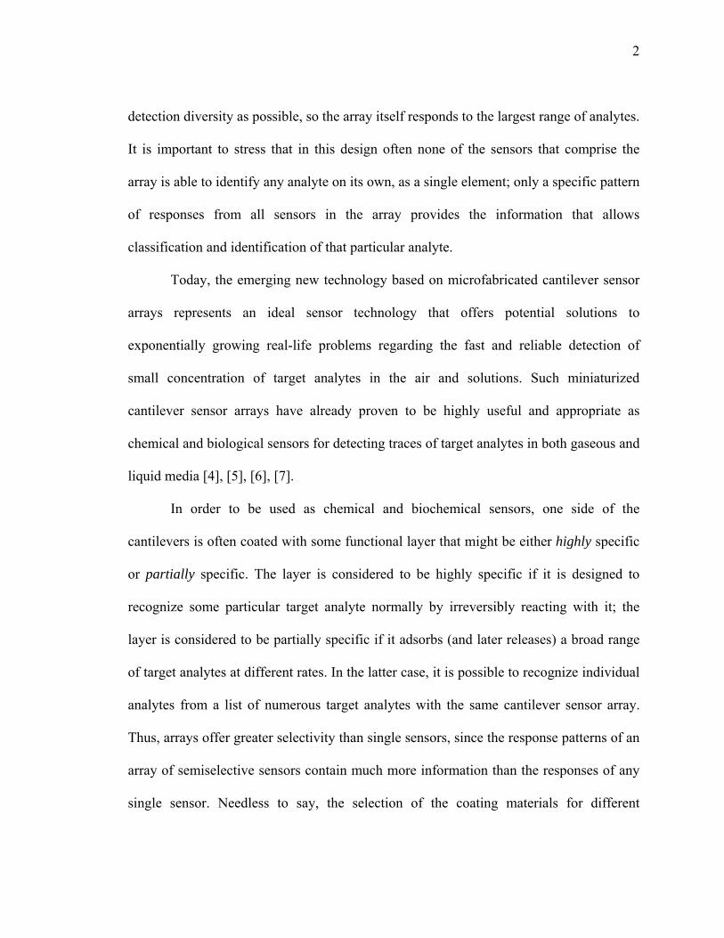
detection diversity as possible, so the array itself responds to the largest range of analytes.
It is important to stress that in this design often none of the sensors that comprise the
array is able to identify any analyte on its own, as a single element; only a specific pattern
of responses from all sensors in the array provides the information that allows
classification and identification of that particular analyte.
Today, the emerging new technology based on microfabricated cantilever sensor
arrays represents an ideal sensor technology that offers potential solutions to
exponentially growing real-life problems regarding the fast and reliable detection of
small concentration of target analytes in the air and solutions. Such miniaturized
cantilever sensor arrays have already proven to be highly useful and appropriate as
chemical and biological sensors for detecting traces of target analytes in both gaseous and
liquid media [4], [5], [6], [7].
In order to be used as chemical and biochemical sensors, one side of the
cantilevers is often coated with some functional layer that might be either highly specific
or partially specific. The layer is considered to be highly specific if it is designed to
recognize some particular target analyte normally by irreversibly reacting with it; the
layer is considered to be partially specific if it adsorbs (and later releases) a broad range
of target analytes at different rates. In the latter case, it is possible to recognize individual
analytes from a list of numerous target analytes with the same cantilever sensor array.
Thus, arrays offer greater selectivity than single sensors, since the response patterns of an
array of semiselective sensors contain much more information than the responses of any
single sensor. Needless to say, the selection of the coating materials for different

3
cantilevers in the array, in order to increase the sensor array’s ability to detect a larger
number of individual analytes or to analyze mixtures, is yet another challenge that this
sensor technology faces today [8].
The response of the cantilever array has to be analyzed via some pattern
recognition technique, which aims to facilitate the application of the device as a reliable
and inexpensive sensing system. Today, pattern recognition is a critical part of the
development of the micromechanical cantilever arrays of sensors capable of detecting,
identifying and sometimes quantifying the target chemical and biological substances. The
successful design process involves a careful consideration of a lot of different issues,
such as signal preprocessing, feature extraction, feature filtering and selection, designing
of the pattern analysis system, training the system, and finally performing recognition of
future (unseen before) samples and assessing the results of system’s classification
accuracy [9].
There were several objectives of the current work.
The first objective was to design and conduct a series of experiments with a
microfabricated cantilever sensor array by exposing it to a set of target analytes. During
this stage of the research, we explored the effects of different coating materials, heating
and cooling the array cell, and the different concentrations of the analytes in the air on the
collected sensory data.
The second objective of our work was to develop the process of feature extraction
and selection. In order to create a successfully functioning detection system, we had to

4
carefully choose the adequate number of features and ensure that those features are both
unique and sufficient to characterize each collected sample during the experiment.
The final and most important objective of the current work was to develop a
number of suitable pattern recognition algorithms for our specific sensory data, test those
algorithms using the benchmark data sets and data collected within framework of the
current research, compare their efficiency and accuracy, and make necessary assessment
of their power and suitability for the detection of the target analytes with a
microcantilever sensor array in the real-life situations.
This thesis is structured as follows:
Chapter 2 − Related Work: presents a review of the current progress in the field
of the microcantilever sensor array technology. It also describes the types of
pattern recognition algorithms that are often used in combination with
microcantilever sensor arrays for the detection and qualitative and quantitative
identification of a wide range of the target analytes.
Chapter 3 − Experimental Setup: describes the details of the experiments
conducted with a microcantilever sensor array, shows some pictures of the array’s
responses, and explains the strategy of the feature extraction procedure.
Chapter 4 − Theory and Algorithms Details: presents a theoretical background
and detailed description of all pattern recognition algorithms that were designed
and implemented in the current research. It also shows the testing results of
classification accuracy for each algorithm using a benchmark data set (the
Wisconsin breast cancer data set).

5
Chapter 5 − Experimental Results: contains the results of each algorithm’s
performance on the experimental sensory data collected in the Nevada Nanotech
System, Inc. (NNTS) laboratory using a microfabricated cantilever sensor array.
Chapter 6 − Conclusion and Future Work: summarizes the performance results
of all pattern recognition algorithms on the given sensory data set and provides
some suggestions for future work in the most promising directions.

6
2 Related Work
Microcantilevers constitute a special class of sensors – mechanical sensors, also
called deflection sensors, meaning that those sensors respond to changes of external
parameters, such as temperature changes or molecule adsorption, by a mechanical
response, e.g., by bending or deflection.
The term cantilever means a microfabricated rectangular bar-shaped structure,
whose length is much greater than its width, and thickness is much smaller than both its
lengths and width. Cantilever beams have been used to measure interatomic forces in the
piconewton range using a technique called scanning force microscopy (SFM) or atomic
force microscopy (AFM) since the mid 1980’s [10]. It turned out that microcantilevers
were exceptionally sensitive to extremely low external forces or remarkably small mass
displacements, that is, they were found to be very sensitive to external physical and
chemical influence. Microcantilevers can operate in several modes, the most often used
modes are static and dynamic modes, and potentially provide mass detection at the single
molecule level.
In static mode [11], [12], [13], the cantilever surface (or a coating material of the
upper surface of a cantilever) adsorbs molecules from the environment and the surface
stress occurring during the adsorption results in a static bending of the cantilever and can
be measured.
In dynamic mode [11], [14], [15], [16], each cantilever in the array is driven into
oscillation externally at its unique resonance frequency. The cantilevers may be coated as

7
well. On the adsorption of the molecules from the surrounding medium, the resonance
frequencies of each cantilever decrease due to the adsorbed mass. Those resonance
frequency shifts can be measured and the adsorbed mass on the cantilever can be
calculated.
The key to the high sensitivity of the microcantilevers is the very large surface-to-
volume ratio, which leads to amplified surface stress.
The ability to use the arrays of sensors functionalized differently adds to the list of
their advantages even more, by providing high selectivity toward certain classes of
chemical and biological analytes. Arrays provide more useful and reliable information,
since using many cantilevers in the same experiment opens up the possibility of exposing
several differently functionalized cantilevers and reference cantilevers under identical
conditions, i.e., several experiments can be performed at the same time. Additionally,
none of the sensors in the array has specific selectivity to a given analyte, while it is often
the case that the collective response from all sensors in the array provides the unique
pattern that allows classification and identification of that particular analyte.
As was said before, in dynamic mode, the cantilever oscillates at a resonance
frequency (the cantilever is driven into oscillation by some external circuitry). Analyte
molecules adsorb to the active layer on the cantilever, increasing the mass of the
vibrating cantilever and therefore, causing a light shift in the cantilever vibration
frequency, very well measurable by external means. By measuring the resonance
frequency sifts, the cantilever array can register a wide range of analyte concentrations in
the surroundings.

8
In order to recognize a variety of analytes, or the different individual components
in the mixture of analytes, each cantilever in the array should be coated with a different
material that shows specific response (selectivity) to a particular class of analytes.
Therefore, when arrays are used, it is preferable to use several different coating materials,
each with somewhat different selectivity toward different classes of analytes. This
approach maximizes the collection of the relevant sensor information for detecting and
recognizing the analytes of interest. Due to this, there is high need of polymers suitable as
coating materials for microcantilever sensors, with good physical and chemical properties
for rapid and reversible analyte adsorption.
Both physical and chemical properties of coating polymers are equally important
in making a good sensor. While the chemical properties determine the selectivity of the
sensor to a particular analyte (or a class of analytes), the physical properties play an
important role in other aspects of the performance, such as response time or refreshment
time [8].
A wide variety of polymers has been studied and employed as suitable coating
materials for microcantilever sensors to modify their sensitivity and selectivity to the
target analytes. Some of the commercially available polymers that have been used in the
current work are the following [8], [17], [18]:
1) PDMS (polydimethylsiloxane) – nonpolar polymer:
Si
Me
Me
O
n
It is known to be useful for adsorbing aliphatic hydrocarbons or for
distinguishing between members of a homologous series.

9
2) BSP3 (phenolic and trifluoromethyl groups added to dimethylsiloxy-polymer chain) –
strong hydrogen bond acidic polymer:
Si
Me
Me
O Si
Me
Me
O Si
Me
Me
OH OH
CF3
CF3
n
This type of material is useful in detection of basic vapors including organophosphorus
compounds (some nerve agents are in that category).
3) OV-275 (poly(biscyanoallyl)siloxane) – dipolar moderately basic polymer:
SiO
CN
CNn
This polymer helps to distinguish vapors with a large dipole
moment.
4) PECH (poly(epichlorohydrin)) – moderate dipolar polymer, contains moderate
hydrogen-bonds:
O
Cl
n
This coating material appears to be good at detecting aromatic
hydrocarbons, such as benzene and toluene.
In addition to the demand of using different coating materials for different
cantilevers within an array, normally at least one cantilever should be left uncoated to

10
serve as internal reference. All these factors and an extremely small size of the
cantilevers themselves constitute a great challenge to functionalize cantilevers in the
array individually [19]. There are not many suitable technologies available to do that.
Among the most successful ones are coating the cantilevers using electrospray [20], [21]
and inkjet printing [22]. The latter method was used in the process of functionalization of
the cantilever sensor array used and tested in the current work (coating of the array
cantilevers was performed by the Nevada Nanotech System, Inc. (NNTS) staff).
Several methods to monitor cantilever deflection have been successfully used in a
measurement setup for cantilever arrays. These methods include optical (external laser)
detection [23], [24], integrated piezoresistive detection [25], [26], integrated capacitive
sensing [27], [28], and piezoelectric methods [29], [30], [31]. Piezoelectric cantilevers are
ideal for resonance, frequency-based approaches – they do not require external optics or
actuators, have low-power consumption, and allow actuating each cantilever in the array
independently and directly. Therefore, the piezoelectric cantilever sensor array was used
in the current work [32].
Creating sensitive, selective, reliable, robust, low-power and low-cost
microcantilever sensor arrays is only a part of the solution to the global problem of
detection of the target chemical and biological substances. Without dependable, fast, and
accurate pattern recognition algorithms we would not be able to use such devices for the
detection of any analytes of interest. Thus, the most important and crucial part in the
development of a sensor array capable of detecting, identifying, and measuring the target
analytes remains the development of a suitable pattern recognition algorithm.
11
The goal of a pattern recognition algorithm is to generate a class label prediction
for a previously unseen sample from a set of class labels learned during the training phase
of the algorithm. Obviously, in order to be able to recognize an analyte, the pattern
recognition algorithm should be trained on a sufficiently large set of data. By data here
we mean the output of any observation or measurement recorded by the cantilever sensor
array under exposure to the target analyte (or a mixture of analytes) and by sufficient data
we mean that in general, it is desirable that the algorithm be introduced to samples from
all possible classes or categories. Then, by exploiting the knowledge extracted from the
training data, the learning algorithm should be capable of adapting itself to infer a
solution to the task of recognizing a new sample as belonging to some previously seen
class (or several classes).
Perhaps the most widely exploited pattern recognition algorithms used in
combination with cantilever sensor arrays are principal component analysis (PCA) [33],
[34], [35], [36], [37] and a variety of neural networks (ANNs) [34], [36], [38], [39], [40].
In all cases satisfactory classification results were reported.
Principal component analysis extracts features from the observed data that exhibit
the most dominant deviations in responses to various analytes. This procedure is aimed at
maximum distinction performance between analytes. PCA in combination with cantilever
sensor arrays was used, for example, to detect primary alcohols in gaseous mixtures [34],
to detect and recognize vapors of dichloromethane, ethanol, toluene, and water in the air,
and also perfume essences and beverage flavor [35], to detect different individual
components such as methanol and 2-propanol in their binary mixtures [36]. PCA was also

12
used to find the best coating materials (out of 27) to successfully recognize one out of 14
analytes [37] – it has been found that only 7 different coating materials are required to
discriminate among those 14 analytes.
For more complex measurements, e.g. to analyze multicomponent mixtures of
gaseous analytes such as natural flavors, a different strategy involving artificial neural
networks is pursued. Whereas PCA extracts most-dominant differences in the fingerprint
pattern, neural network analysis considers all components of the fingerprints. Among the
most interesting examples of the use of artificial neural networks are the detection and
identification of different odorants (organic vapors such as amyl acetate, acetoin,
menthone, and some aliphatic alcohols) [39], the identification of organic solvents in
binary mixtures (n-octane − chloroform, n-octane − n-propanol, chloroform −
n-propanol) [40]. The results for classification accuracy obtained by neural networks vary
greatly, between 70% and 100%.
Among other pattern recognition techniques reported to be used in combination
with cantilever sensor arrays is principal component regression (PCR) that was used, for
example, for the quantitative prediction of organic vapors of octane, toluene, ethanol, and
butylamine in the binary mixtures; the prediction error of 11.8%−12.5% is reported [41]
and for quantitative and qualitative analysis of organic vapors of n-octane, 1-butanol, and
toluene in binary mixtures high accuracy of the detection is reported [42].
The fuzzy c-means clustering algorithm (FCM) was used for the discrimination of
organic compounds (14 different analytes total) [43]. The fuzzy c-means algorithm has
13
been found to perform better than PCA in discriminating analytes with similar structure,
such as benzene and toluene, homologous alcohols, and acyclic aliphatic hydrocarbons.
Some modifications of PCA for multivariate data for the application to sensor
arrays, such as Independent Component Analysis (ICA) – for the detection of different
concentration of propanol and ethanol [44] and for identifying the concentration of
carbon dioxide and hydrogen in the mixture [45], and Principal Discriminant Analysis
(PDA) – for the discrimination among five varieties of roasted coffee beans are also
reported [46]. The results of classification accuracy for ICA were reported as satisfactory,
whereas PDA performed only with 64% of classification rate on coffee beans.

14
3 Experimental Setup
3.1 Experimental Setup
The experimental part of the current work was performed in the laboratory of
Nevada Nanotech Systems, Inc. (NNTS).
Figure 1 shows the basic experimental setup for collecting sensory data during
exposure of the microcantilever sensor array to the gaseous mixture containing an
analyte.
Figure 1. Basic experimental setup.
Flow rate controller Flask with an analyte Cell temperature controller

15
The flow rate control system allows us to create and maintain the desirable
concentration of an analyte in the gaseous mixture (Figure 1, Figure 2) that the
microcantilever sensor array (Figure 4) has to be exposed to. The dry air was forced to
flow under excess pressure through a flask with an organic solvent (the chemical analyte)
and the gaseous mixture of the dry air highly saturated with vapors of the given analyte
was subsequently diluted several times until the needed concentration of an analyte in the
air was reached.
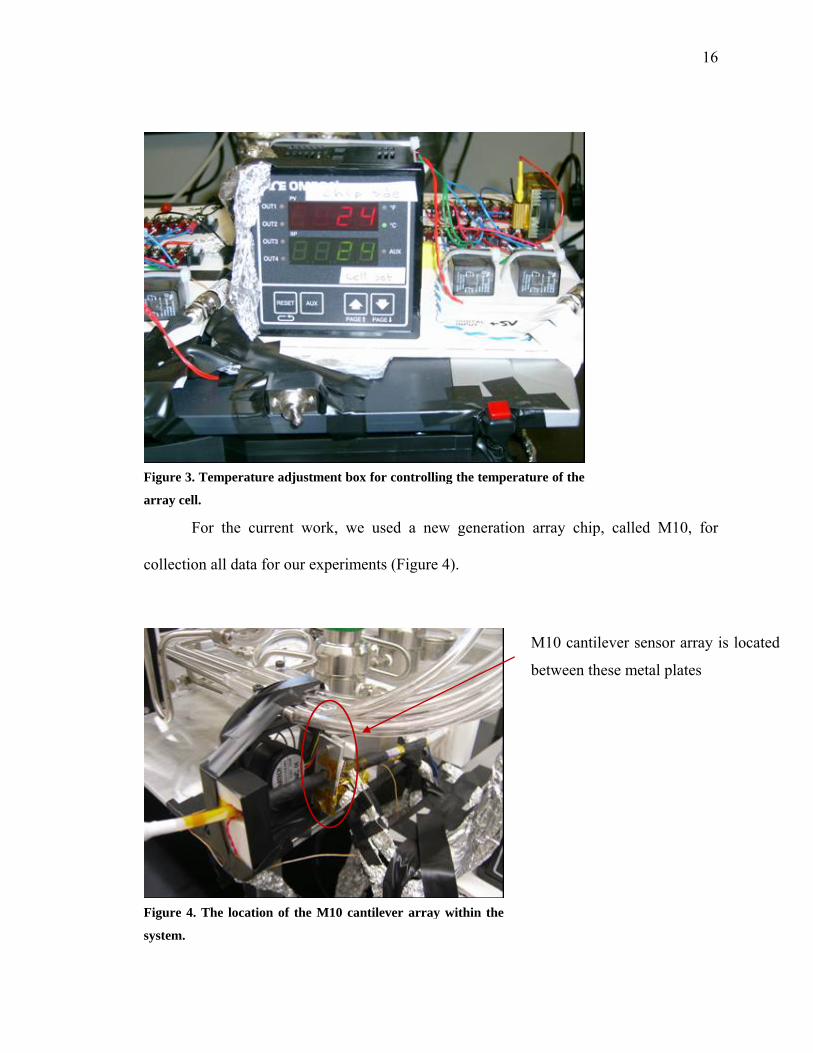
During the experiments some heating of the microcantilever array cell was
applied as well. For heating (Figure 3), a different amount of electrical current was
applied to the entire array of the cantilevers (all microcantilever sensors were heated and
cooled simultaneously)
Figure 2. Flow rate control system for controlling the desired concentration
of the chemical vapors.
16
For the current work, we used a new generation array chip, called M10, for
collection all data for our experiments (Figure 4).
Figure 3. Temperature adjustment box for controlling the temperature of the
array cell.
M10 cantilever sensor array is located
between these metal plates
Figure 4. The location of the M10 cantilever array within the
system.
17
Theoretically, this array has a large number of cantilevers, but only one row of
them (ten cantilevers total) was wire-bonded and seven out of these ten cantilevers were
coated with seven different coating materials. The remaining cantilevers were left
uncoated.
The polymers that were used for coating the cantilevers and their respective
chemical properties are:
OV275 dipolar, moderately basic polymer
PDMAEMC strong basic polymer
PBM dipolar, basic polymer
PDPZ polarizable polymer, contains phenyl groups
PECH moderate dipolar polymer, contains moderate hydrogen-bonds
PDMS nonpolar polymer
BSP3 strong hydrogen-bond acidic polymer
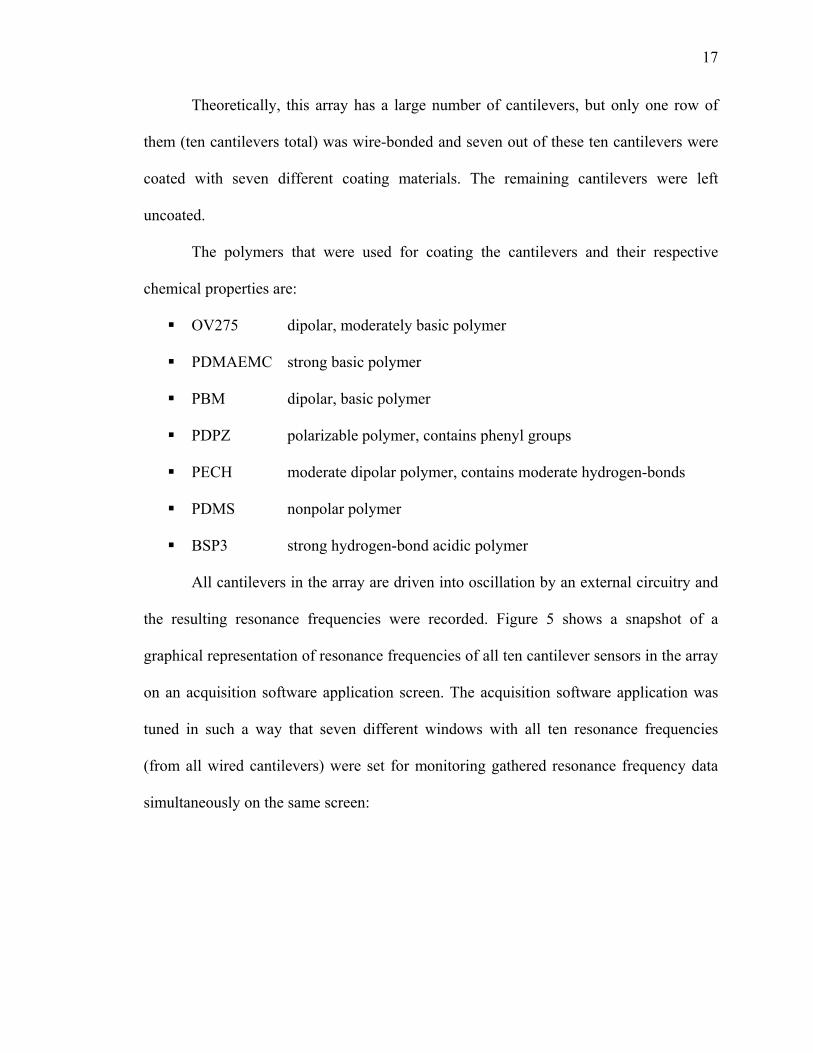
All cantilevers in the array are driven into oscillation by an external circuitry and
the resulting resonance frequencies were recorded. Figure 5 shows a snapshot of a
graphical representation of resonance frequencies of all ten cantilever sensors in the array
on an acquisition software application screen. The acquisition software application was
tuned in such a way that seven different windows with all ten resonance frequencies
(from all wired cantilevers) were set for monitoring gathered resonance frequency data
simultaneously on the same screen:
18
Figure 5. The figure shows a snapshot of all ten resonance frequencies: window 1 – OV275, span 45
kHz; window 2 – uncoated cantilever, span 40 kHz; window 3 – BSP3, span 60 kHz; window 4 –
uncoated, uncoated, PBM, PDMAEMC, span 135 kHz; window 5 – PDPZ, span 45 kHz; window 6 –
PECH, span 45 kHz; window 7 – PDMS, span 50 kHz.
3.2 Experiment Protocol Description
To calibrate our system, we ran a series of temperature experiments. The data
were collected at five different temperatures: room temperature, 24, 28, 32, and 36°C (the
thermo caps were set at the front and at the back of the array cell, so the temperature was
measured with high precision).
In order to control the temperature during the experiment, special hardware
consisting of a heater and fan was developed. The fan is automatically activated and the

19
heater is automatically set off if the temperature goes higher than desired; likewise, the
heater is automatically set on and the fan is automatically set off if the temperature goes
below the settings.
The objectives of the temperature experiments were the following:
get stable and reproducible response of all cantilever at each temperature;
make sure that the entire array is kept at designated temperature during the entire
experiment (hardware issues);
find the temperature–resonance frequency shift dependence for all cantilevers (so
that we can use this information in the future to estimate how much the high
temperature contributes to resonance frequency shifts of different cantilevers in
some ambiguous situations).
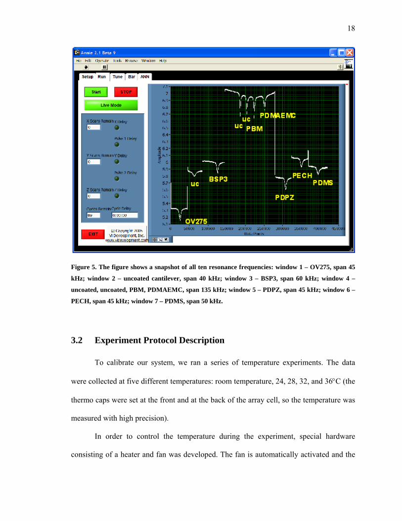
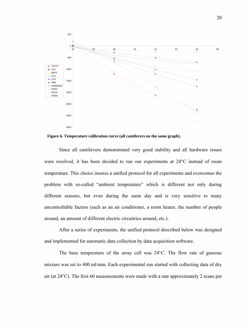
This series of experiments resulted in the temperatures calibration curves shown
in Figure 6:
20
Since all cantilevers demonstrated very good stability and all hardware issues
were resolved, it has been decided to run our experiments at 24°C instead of room
temperature. This choice insures a unified protocol for all experiments and overcomes the
problem with so-called “ambient temperature” which is different not only during
different seasons, but even during the same day and is very sensitive to many
uncontrollable factors (such as an air conditioner, a room heater, the number of people
around, an amount of different electric circuitries around, etc.).
After a series of experiments, the unified protocol described below was designed
and implemented for automatic data collection by data acquisition software.
The base temperature of the array cell was 24°C. The flow rate of gaseous
mixture was set to 400 ml/min. Each experimental run started with collecting data of dry
air (at 24°C). The first 60 measurements were made with a rate approximately 2 scans per
-3500
-3000
-2500
-2000
-1500
-1000
-500
0
500
24 26 28 30 32 34 36 38
OV275UC1BSP3UC2UC3PBMPDMAEMCPDPZPECHPDMS
Figure 6. Temperature calibration curve (all cantilevers on the same graph).
21
minute; the remaining 240 measurements were taken without any delay (approximately 2
scans per second). Between the 11th and 12th scans, the chemical vapors were introduced
into the gaseous mixture (we used only three different concentrations of the chemical
vapors: 7%, 18%, and 26%). Approximately 40-42 measurements were taken at very high
temperature (the electrical impulse was applied to cantilevers between scans 121-123 and
164-166, estimated temperature was 100-150°C); after removing the heat, the remaining
approximately 135 measurements were taken while the array was cooling to 24°C.
After a cycle of the experiment with the chemical vapors was over, the next cycle
was a “refreshment run.” During this refreshment run the protocol was almost the same
except that halfway between the 11th and 12th scans the chemical vapor gaseous mixture
was replaced by the dry air and the entire array was heated at 55°C to speed up the
desorption process of the analyte molecules from the polymer layers (during the
refreshment cycle data were collected as well).
The protocol of the experiments with chemical vapors was designed in such a way
so that we collect as much versatile information as possible:
how fast different cantilevers start reacting with the introducing of a specified
concentration of the specified chemical vapors;
how fast the cantilevers get into the “steady” state (the resonance frequency is not
changing any more);
what happens during heating, cooling down, etc.
Besides impedance and resonance frequency shifts, we also measured the peak
heights of each frequency during each scan (we assumed that it might be a valuable
feature as well for our feature vectors).

22
Another positive characteristic of the above protocol was that the data did not
depend on the baseline information, which might be recorded under slightly different
conditions every time it was needed. In our experiments, we used the very first scan in
each run as a baseline for the remaining 299 scans. By doing so, we measured only the
relative changes during each experiment (we didn’t have an impact of a so-called
“accumulation” factor, when the baseline was getting further and further from the current
plot, since the array never had a chance to be completely refreshed during the entire day
of the experiments and it didn’t completely release everything it accumulated during each
run).
3.3 Data Collection Results
For the current work, we conducted experiments using vapors of different
concentration (7%, 18% and 26%) of three different chemicals: acetone, toluene and
ethanol. Figure 7 − Figure 12 show the responses of the cantilever array from some of
these experiments.

23
Figure 7. Resonance frequency shifts of all cantilevers during exposure of the array to 18% of
acetone.
Figure 8. Heights of resonance frequency peaks of all cantilevers during exposure of the array to
18% of acetone.

24
Figure 9. Resonance frequency shifts of all cantilevers during exposure of the array to 7% of
ethanol.
Figure 10. Heights of resonance frequency peaks of all cantilevers during exposure of the array
to 7% of ethanol.
25
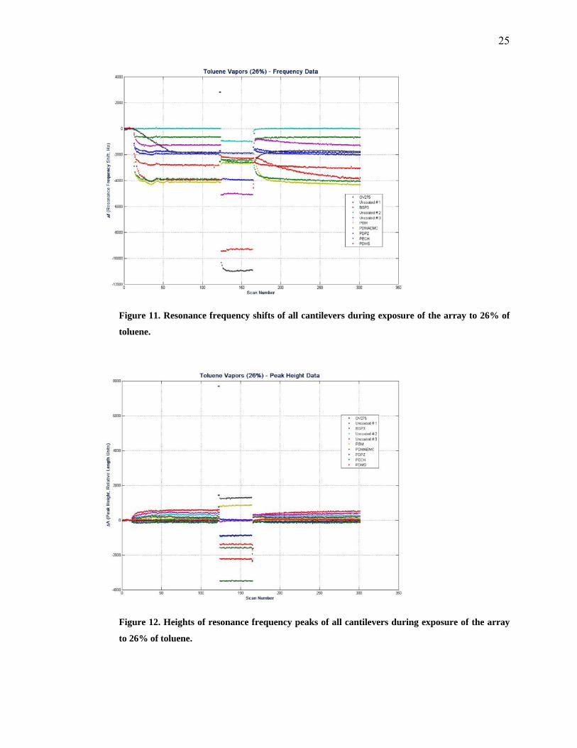
Figure 11. Resonance frequency shifts of all cantilevers during exposure of the array to 26% of
toluene.
Figure 12. Heights of resonance frequency peaks of all cantilevers during exposure of the array
to 26% of toluene.

26
3.4 Feature Extraction
While running the experiment, our system takes different measurements
according to the protocol described above (such as resonance frequency, impedance) and
saves them into an output file. After processing this file using a peak finding routine (this
program was created by Dr. Jesse Adams from NNTS), a file consisting of almost 7000
different measurements is created. For each cantilever there are 300 values of the
resonance frequency shifts measured at specified time points, 300 values for the peak
heights of each resonance frequency peak, and the rest of the data is impedance
information, which has been measured in several chosen points along the baseline of
several cantilevers.
In order to reduce the amount of information to be processed, we extracted a
subset of values from the total of 7000 pieces of data by applying our knowledge of the
input domain (will be explained shortly), which helps create a feature vector that fully
characterizes the gaseous mixture along with the conditions of the experiment.
In the current work we used data recorded for the following cantilevers:
cantilevers coated with OV275, BSP3, uncoated cantilever # 3, cantilevers coated with
PBM, PDPZ, PECH, and PDMS. Thus, we used the information obtained by only seven
out of ten cantilevers. We left out the data collected by the cantilever coated with
PDMAEMC and the remaining two out of three uncoated cantilevers, because these three
sensors provided very inconsistent information. Possibly, that could be due to some
physical defects of these three cantilevers, such as some foreign body like a piece of fiber
lying on the sensor, or in the case of PDMAEMC, the uneven coating or the unknown

27
properties of this polymer that easily accumulates but not so easily releases the molecules
of certain chemicals.
Figure 13 − Figure 15 illustrate the strategy that we used to extract the most
prominent features from the resonance frequency responses of the cantilever sensors in
the array.
Figure 13. The figure shows the measurements for resonance frequency of the cantilever coated with
OV275 polymer taken according to the protocol (described above). Red bidirectional arrows
represent the difference taken before and after some conditions were changed, red curly braces
indicate the areas on the graph where the row data as an average over 10-20 points were used.
28
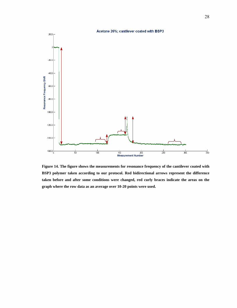
Figure 14. The figure shows the measurements for resonance frequency of the cantilever coated with
BSP3 polymer taken according to our protocol. Red bidirectional arrows represent the difference
taken before and after some conditions were changed, red curly braces indicate the areas on the
graph where the row data as an average over 10-20 points were used.
29
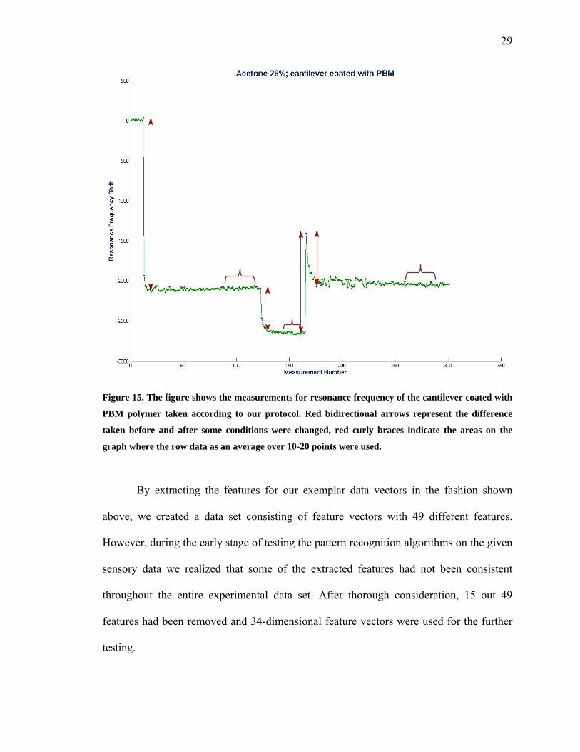
Figure 15. The figure shows the measurements for resonance frequency of the cantilever coated with
PBM polymer taken according to our protocol. Red bidirectional arrows represent the difference
taken before and after some conditions were changed, red curly braces indicate the areas on the
graph where the row data as an average over 10-20 points were used.
By extracting the features for our exemplar data vectors in the fashion shown
above, we created a data set consisting of feature vectors with 49 different features.
However, during the early stage of testing the pattern recognition algorithms on the given
sensory data we realized that some of the extracted features had not been consistent
throughout the entire experimental data set. After thorough consideration, 15 out 49
features had been removed and 34-dimensional feature vectors were used for the further
testing.

30
We also made several attempts to include more features in our vectors, such as
polynomial coefficients given by a curve fitting procedure and height values of resonance
frequency peaks. As we can see from the provided graphs, there are some areas that
correspond to changing the temperature of the array cell (points 123-130, 165-175 – both
parts of the curves fit nicely into polynomial of degree 3) or to introducing the chemical
vapors in the air (points 12-20 – this part of the graph fits into polynomial of degree 2)
that could be used as features in our feature vectors. We hoped that by adding more
unique features to the feature vectors, we might significantly improve the classification
accuracy of our algorithms. However, it turned out that those features (polynomial
coefficients and peak heights) were inconsistent and unreliable from the experiment to
experiment and instead of adding the additional distinctive characteristic, those features
added more ambiguity and uncertainty.
In the end we kept the features that most closely described a variety of states that
the cantilevers went through during the experimental run. Among the features we kept in
our feature vectors were: 1) changes of the resonance frequency values after introducing
an analyte into the air and after applying and removing the heat, and 2) the resonance
frequency shifts of the cantilevers, averaged over several measurements during the steady
states of the cantilever array before applying the heat, during the heating process, and at
the end of the experiment when the array was cooled down to 24°C.
31
4 Theory and Algorithms Details
The ultimate goal of our research was to create a reliable algorithm that after
training on a limited set of labeled feature vectors from various classes can recognize any
unseen feature vector as belonging to one of these classes (or even more than one class,
but with a different degree of confidence).
Therefore, we needed to create a reliable classifier system that could use a
learning algorithm (or some combination of various learning algorithms) to gain enough
knowledge about the problem domain to be able to correctly recognize any unseen
sample afterwards. Thus, we had to successfully solve two separate problems: (1) to
make our system learn from a limited pool of labeled pieces of data and (2) to teach our
system to correctly label any number of new, unseen and therefore unlabeled samples
from the same problem domain. Sometimes an algorithm includes solutions to both
problems (learning and classification) at once; sometimes we have to seek different
algorithms for each problem independently.
Machine learning and classification methods for pattern recognition are extremely
versatile. Among them we can mention the most popular ones, such as Principal
Component Analysis (PCA) [47], [48], and Multiple Discriminant Analysis (MDA) [49],
probabilistic neural networks (PNNs) [50], [51], [52], [53], [54], radial basis function
neural networks (RBFNNs) [55], [56], [57], [58], [59], crisp and fuzzy clustering [60],
[61], [62], [63], [64], Support Vector Machines (SVMs) [65], [66], [67], [68], [69] and
genetic algorithms (GAs) [70], [71], [72], [73], [74].

32
Below are some definitions and notations that will be used throughout the rest of
this work.
A feature vector (pattern, object) xr is a single data item in the data set under
observation. Typically, it is a vector in the N-dimensional vector space Nℜ :
),...,,( 21 Nxxxx =r . Each individual scalar component ix of vector xr is called a feature
(attribute, dimension, or variable). A data set of Q feature vectors is denoted
},...,,{ 21 QxxxX rrr= or },...,2,1:{ )( QqxX q ==
r , where the q-th feature vector in X is
denoted ),...,,( )()(2
)(1
)( qN
qqq xxxx =r . A class is a certain category of the objects (feature
vectors) that has some unique or distinctive characteristics that easily distinguish it from
other classes in the set. A feature vector can be labeled, meaning that we are provided
with the information to which class the particular feature vector belongs, or unlabeled,
meaning that we do not know this type of information.
The notion of a feature vector proximity measure is fundamental for all
algorithms we used in the current research. We used the Euclidean distance as a measure
of similarity between two feature vectors drawn from the same feature space:
( ) ||||),( )()(
0
2)()()()( rqN
i
ri
qi
rq xxxxxxd rrrr−=−= ∑
=
( 1 )
In order to find the best possible solution to our problem of classifying specific
sensory data, we implemented several learning and classification methods and tested
them on a well-known benchmark data set, the Wisconsin Breast Cancer Database that
contains 699 9-dimensional feature vectors (instances of two classes − malignant and
benign) [75]. The feature vectors of the entire data set have been standardized
33
independently for each feature, so that they belong to the hypercube [0,1]N (N is
dimension of the feature space), which permits each feature to have the same influence
on the classifier systems. 7-Fold cross validation of the Wisconsin Breast Cancer Data
Set has been used to tune the parameters and evaluate classification accuracy for all
algorithms we used in the current work. Thus, this data set has been divided into seven
training/testing set pairs (six pairs of sets containing 599 feature vectors in the training set
and 100 feature vectors in the testing set and one pair of sets containing 600 feature
vectors in the training set and 99 feature vectors in the testing set).
4.1 Extended Classifier System (XCS)
XCS, a recently developed classifier system in the context of Evolutionary
Computing [74], bases its fitness function on classification accuracy and implements so-
called reinforcement learning. XCS creates and maintains the population of classifiers,
each of those classifiers maintains its own prediction of the expected reinforcement
(“payoff,” “reward”) from the environment. XCS executes the genetic algorithm (GA) in
the environmental niches defined by the match to the given input sent by the
environment, instead of using random mating and mutation within the entire population
of classifiers. As a result, XCS tends to evolve the classifiers that are not only highly
accurate, but also are maximally general. By "general classifier," we mean a classifier
that considers inputs that have the same consequences on the environment as identical.
With this, a general classifier captures regularity in the environment and by incorporating
"don't care" symbols is capable of matching more than one input vector. [76], [77].
There are several main aspects of XCS that should be emphasized.
34
First, XCS is a learning machine, that is, a learning program within a computer.
Its behavior significantly improves over time through interaction with the environment
that constantly sends feedback on XCS’s performance.
Second, XCS learns on-line, meaning that it cannot collect a lot of experience in
some temporary storage and then process all the collected information. Instead, it learns
as it goes along – it extracts the implication of every single experience as it occurs.
Third, XCS tries to capture regularities of the environment. This means that XCS
tries to create not only accurate classifiers, but also general ones. By generality of the
classifier we mean that it holds the knowledge about some part of the problem space (not
only about a single representative of that space) being maximally accurate at the same
time. A machine with even a small number of sensors will encounter an enormous
number of sensory states in any reasonably complicated environment. Thus, it is
extremely important for the learning algorithm to be able to capture the similar behavior
of the environment and group the states of the environment having the same implication
for its behavior. Thus, generalization is a core of XCS. Because of generalization, XCS
has an intrinsic tendency to evolve accurate, maximally general classifiers [77].
Furthermore, XCS learns to get reinforcements, in other words, it learn to act in
such a way that it always receives maximally possible rewards from the environment.
Often, it is very difficult to “explain” to the machine what it should do in order to achieve
some goals that we set for it. Instead, it is much easier to establish the framework of
reinforcement learning – every time the machine does something that we want we give it
a reward. This way, we are leaving for the machine to figure out by itself what exactly it
should do in order to be rewarded.

35
Thus, XCS acts as a reinforcement learning agent: it receives an input that
describes the current state of the environment and reacts on the given input by emitting
some actions, which are immediately sent back to the environment. This action can affect
the environment and may result in some payoff. For this work, we restrict inputs from the
environment to binary strings. The input space is denoted by LS }1,0{⊆ , where L is the
length of the input string. XCS’s knowledge is contained in a set of condition-action rules
called classifiers. Each classifier consists of a condition part, an action part, and a
prediction part. The condition LC }#,1,0{∈ specifies which input states Ss ∈ the
classifier can match (“#” is a “don’t care” symbol). The action a specifies the action that
the classifier has chosen and expected a payoff. Classifier’s prediction p can be defined
as an average of the payoff received (internal or external, or some combination of both)
when the classifier’s action controls the system. Among other important XCS’s attributes
are the following: prediction error ε (an average of a measure of the error in the
prediction parameter) and fitness F, which estimates the accuracy of the payoff
prediction p (normally, F is some inverse function of the prediction error that basically
represents the classifier’s accuracy; therefore, the XCS’s fitness calculation is entirely
based on its classification accuracy).
Since there are many classifiers within the system at any time (perhaps,
hundreds), after XCS has been trained for a while, it will contain the classifiers that
accumulate the knowledge about all parts of the input and action space that it has
experienced so far. This ability to accumulate the meaningful knowledge in some limited
set of classifiers makes XCS unique compared to other types of learning machines. In
36
XCS, the knowledge about some chunk (could be very considerable) of the problem
space is contained in individual classifiers (sometimes, even in only one of them). We
can take a classifier out of the context of the entire system and learn a lot about some
particular subspace of the problem space. In contrast, the knowledge about some problem
in the neural network, for example, is distributed over the whole network, all its nodes
and node’s weights, and nothing in this network taken separately can tell us anything
useful about the problem it has learned.
4.1.1 Performance of XCS
For the following discussion, we assume that the population [P] of the classifiers
is not empty. XCS interacts with the environment as follows.
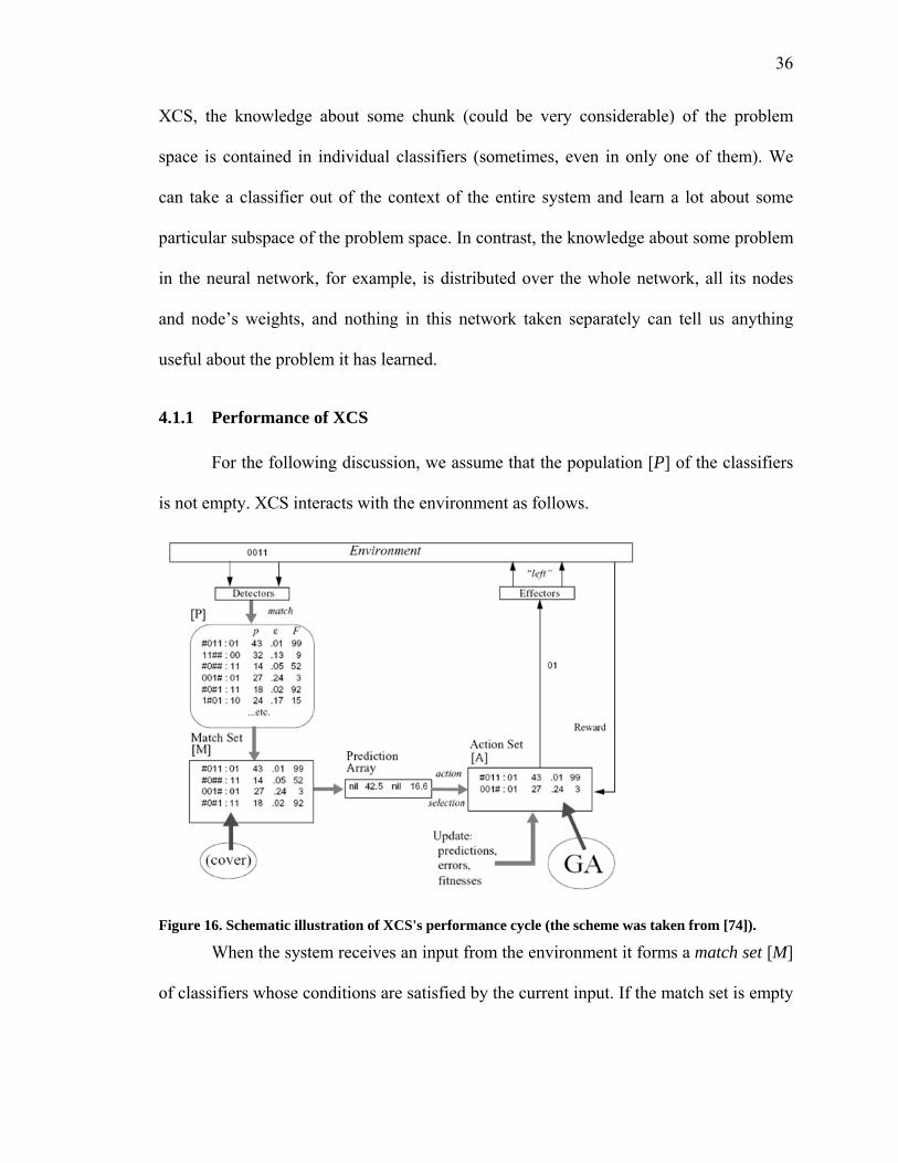
Figure 16. Schematic illustration of XCS's performance cycle (the scheme was taken from [74]).
When the system receives an input from the environment it forms a match set [M]
of classifiers whose conditions are satisfied by the current input. If the match set is empty

37
or it contains less than some specified number θmna of classifiers with different actions,
covering classifiers are created with a condition that matches the current input and some
random action. Specifically, each attribute in the condition of a covering classifier is set
to “#” with a probability P# and to the corresponding input symbol, otherwise. For each
action aj in [M], XCS computes the system prediction array P(aj), which is an estimate of
the payoff that the system expects when action aj is performed. The prediction array is
computed by the fitness-weighted average of all matching classifiers that specify action
aj.
XCS often selects an action with respect to the values in the prediction array.
Even though it seems that XCS should always pick an action that has the highest
prediction in the prediction array, XCS must sometimes choose apparently sub-optimal
actions, in order to be sure that the apparently optimal classifiers are in fact optimal. This
is an example of the explore/exploit dilemma. The system would like to choose the best
action all the time in order to maximize the payoff, but it cannot determine the best action
without sampling other actions as well. The system may simply pick the action with the
largest prediction (deterministic action selection). Alternatively, the action may be
selected probabilistically, with the probability of selection proportional to P(ai) (roulette-
wheel action selection). In some cases the action may be selected completely at random
(from actions with non-null predictions).
In the current work, we have implemented an advanced scheme of action
selection – the gradient change of the explore/exploit rate during the training phase. For
this purpose, the entire training set was divided into four (uneven) partitions so that the
different explore/exploit rates could be applied to meet the needs of the classifier system

38
(e.g., at the beginning of the training phase, when there are none of experienced
classifiers, the higher explore rate should be used, and so on). Exploration experience
(EE) parameter also could be viewed as the number of inputs from the training set
processed so far.
rate 1rate 2rate 3rate 4
Exploration Experience (EE)
Training Set
EE/n1 EE/n2
1 Q
Figure 17. New flexible scheme for action selection that can be finely adjusted to each specific
problem space.
Once the action is selected, the system forms an action set [A] consisting of the
classifiers in [M] advocating the chosen action. An immediate reward R may (or may not)
be returned by the environment.
4.1.2 Reinforcement Component
XCS’s reinforcement component consists in updating the p (prediction),
ε (prediction error), and F (fitness) parameters of classifiers once the reward R is
obtained from the environment.
In the literature, there are a lot of discrepancies and confusion about how exactly
(and in what order) all the classifier’s parameters should be updated. We had performed
several experiments that vary the order of the updates, and some different schemes of
calculating the updated parameters and came up with the solution that we think is the
best. The following approach in executing the reinforcement component of XCS has been
39
established and confirmed by the experiments (our scheme mostly agrees with the order
of updates listed in [77]; but in contrast we update the parameters of those classifiers,
which have not been tested a particular number of times, differently compare to the
conventional way):
1. The current prediction error is calculated:
|| jj pP −=ε ( 2 )
where jε is a prediction error of the j-th classifier, P is a payoff from the environment, pj
is a prediction of j-th classifier.
2. The prediction error is updated based on the classifier experience (the number of time
the classifier has been selected to be in [A]). If its experience is less than some
specified threshold, then εj is an average of all previous values of this classifier’s
prediction errors and the current one. Otherwise:
)|(| jjjj pP εβεε −−×+← ( 3 )
where β (0 < β < 1) is the learning rate.
3. Classifier’s accuracy kj is computed. There are several popular functions for
computing classifier’s accuracy. We had tried the following three functions in our
experiments:
(a) ν
εε
α−
⎟⎟⎠
⎞⎜⎜⎝
⎛×=
0
jjk ( 4 )
if εj > ε0
otherwise, kj = 1

40
(b) ⎥⎥⎦
⎤
⎢⎢⎣
⎡⎟⎟⎠
⎞⎜⎜⎝
⎛ −×=
0
0lnexpε
εεα j
jk , if εj > ε0
otherwise, kj = 1
(c) νε −= jjk , if εj > ε0
νε −= 0jk , otherwise
where α (0 < α < 1), ε0 , and ν (ν ≈ 5) are special constants set by the programmer.
From our tests, we observed that function (a) outperformed the other two. Thus, we
successfully used that function (Eq. 4) in our implementation.
4. The classifier’s relative accuracy is computed for each classifier by dividing its
accuracy by the total accuracies in the set [A]:
∑=
ii
jj k
kk ' ( 5 )
5. The relative accuracy is used to adjust the classifier’s fitness Fj. Fitness is updated
differently based on classifier’s experience in [A]. If this classifier has been adjusted
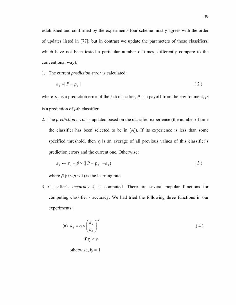
Figure 18. The classifier’s accuracy as a function of the classifier prediction error εj (Eq. 4) (the graph
was taken from [77]).

41
for a specified number of times (i.e., its experience exceeds the threshold value),
then:
)( 'jjjj FkFF −×+← β ( 6 )
Otherwise, Fj is set to the average of the current and previous values of 'jk .
6. Prediction itself is updated (again, based on classifier’s experience); if the classifier is
not experienced enough, pj is calculated as an average of all previous values of this
classifier’s prediction and the current one. Otherwise:
)( jjj pPpp −×+← β ( 7 )
where β (0 < β < 1) is the learning rate.
The idea behind the accuracy calculation is visualized in Figure 18: ε0 is a
threshold measuring the extent to which errors are accepted, α causes a strong distinction
between accurate and not quite accurate classifiers, and the steepness of the succeeding
slope is influenced by ν, as well as ε0. Thus, in XCS the classifier fitness is an estimate of
the classifier’s accuracy relative to other classifiers and behaves inverse proportional to
the reward prediction error. Errors below the threshold are regarded as having equal
accuracy.
4.1.3 Discovery Component
From time to time (not always!) a genetic algorithm (GA) is applied to the
classifiers in the current action set [A]. From the beginning, XCS performs the GA in a
niche (first introduced by Booker in 1982 [78]), and it does not use the entire population
of classifiers as many other classifier systems do. The basic idea of a niche GA instead of

42
using the entire population is that it eliminates the undesirable competition that otherwise
occurs between classifiers in different match sets. In addition, crossovers within a niche
are more likely to yield useful classifiers than crossovers between potentially unrelated
classifiers that match in different niches.
The GA selects two parental classifiers with probability proportional to their
fitness; two children are generated by reproducing, crossing, and mutating the parents. In
the current implementation of XCS, we used a simple single-point crossover and two
types of mutation: free mutation [74] and niche mutation [79]. In free mutation, each bit
of the classifier condition is mutated to the other two possibilities with equal probability.
In niche mutation, a classifier condition is mutated so that it still matches the current
input, i.e., a don’t-care symbol is mutated to the corresponding input value, while 0 or 1
is mutated to don’t-care. Niche mutation generally results in a faster convergence time,
whereas free mutation causes broader exploratory behavior, faster knowledge transfer
and, thus, higher robustness. In the current work, we have added one feature to the free
mutation implementation. While testing our implementation, we have noticed that the
system often chooses the very accurate classifiers with a wrong action. To address this
issue, we have modified free mutation in such a way that action is allowed (with some
small probability) be mutated as well. Thus, in the current work, when performing free
mutation, the system can choose from the pool of all available actions, except the one that
the classifier currently posses.
After new classifiers have been created by the GA, they are inserted into the
population [P]. As happens in all the other models of classifier systems, parents stay in
the population competing with their offspring.

43
4.1.4 Deletion Schemes
Since XCS maintains the size of its population of classifiers constant, every time
new classifiers have to be added to the population [P], XCS faces a problem of deletion.
The importance of deletion in XCS used to be underestimated considerably. If in a
standard GA a chromosome can be evaluated (assigned a reasonable fitness value)
immediately, in XCS, however, a chromosome can only be fully evaluated after many
interactions with the environment (when a classifier has considerable experience of being
in [A]).
Because a new classifier must normally be tested on many trials before XCS can
be certain of its fitness, it is a good idea to set its initial fitness to a low default value and
increase it slightly each time it proves itself useful. This way accurate classifiers
gradually increase their chances of participating in reproduction. Bad classifiers (i.e.,
classifiers that are inaccurate or have low accuracy) tend not to increase in fitness and so
tend not to participate in reproduction.
But since all classifiers initially have a low fitness, a bias against low fitness
classifiers is also a bias against new classifiers, both good and bad (accurate and not).
The stronger the bias, the more the system will tend to delete useful new classifiers
before it has the possibility to test them and evaluate how good they are.
To address this problem, we used the advanced deletion approach proposed by
Kovacs in 1999 [80]. This approach considers the probability of deletion of each
classifier to be proportional to the estimate of size [A] (one more parameter that each
classifier updates every time it gets into [A]) until a classifier has been used on some
specified number of trials. After that, the probability of deletion of each classifier is

44
multiplied by the mean fitness over the current population set [P] and is divided by the
classifier’s fitness if and only if its fitness is less than a small fraction δ (specified by a
programmer) of the population mean fitness. This scheme helps to maintain
approximately the same number of classifiers in each niche and to eliminate inaccurate
classifiers that proved to be bad through numerous interactions with the environment. In
addition to using this advanced scheme of deletion in our work, we have added one
additional feature to protect inexperienced classifiers from deletion before they have been
given a chance to be evaluated; which is to start the processing XCS with a fraction of
maximally possible population of classifiers (100 or 200 out of 500, for example).
The presence in the population of accurate, but unnecessarily specialized
classifiers is an undesirable feature of the classifier system. To address this problem, a so-
called subsumption deletion scheme has been implemented in the current work as well.
The approach can be describes as follows: every time a new classifier is created (by
either the GA or by covering), the entire population is scanned to see if there exists a
classifier whose condition logically subsumes the condition of the new classifier, has the
same action and at least the same accuracy. If the test is satisfied, the new classifier is not
injected into the population, but the numerosity (another important parameter of the
classifier) of the classifier that subsumed that is incremented by one.
In order to implement subsumption deletion, we always insert the most general
classifier into the population [P] first. This approach guarantees that less general
classifiers would be subsumed during the insertion into [P] if the possibility arises.
The mention of numerosity parameter brings another important feature of XCS
into light – the notion of macroclassifiers.

45
4.1.5 Macroclassifiers
In XCS, a macroclassifier technique is used to speed processing of matching [P]
against the input vector and provides a clearer and more unambiguous view of population
contents. Macroclassifiers represent a set of classifiers with the same condition and the
same action by means of the numerosity parameter mentioned above. Thanks to the use
of macroclassifiers, the resulting population [P] consists entirely of structurally unique
classifiers, each with numerosity greater than or equal to 1. If a classifier is chosen for
deletion, its numerosity is decremented by 1, unless the result would be 0, in which case
the classifier is removed from [P].
In order to be sure that the system still behaves as though it consists of N regular
classifiers, the functions are written so as to be sensitive to the numerosities, if that is
relevant. For example, in calculating the relative accuracy, the probability of to be deleted
or selected for mating, and so on, a macroclassifier with numerosity n will be treated as
though it represents n separate classifiers.
Thus, the population as a whole is always treated as though it contains N regular
classifiers, though the actual number of macroclassifiers in [P] may be substantially less
than N, which gives a significant computational advantage.
4.1.6 Test Results
Implementation details of the current algorithm are given in Appendix A.
Since XCS intensively uses the random generated numbers, we run each test
using 30 different seeds to randomize the srand() function. Therefore, each result has
been obtained by 210 program runs (7-fold cross validation by using 30 different seeds).

46
For all tests in each category we used the same set of parameters that have been
optimized in the previous testing procedures. For each test we used the same set of seeds:
for i = 0 to i = 29
seedi = 111×i + 17×i
In order to prove the benefits of our advanced gradient exploration rate scheme,
we performed tests using different constant exploration rates first and then we run a series
of tests that uses our gradient exploration rate scheme. Although these are just
preliminary results and the parameters for the gradient exploration rate scheme could be
adjusted even better, we can see that the average result for the best values of
classification accuracy has been improved.

47
Table 1. Results of classification accuracy obtained by using the constant exploration rate.
PARAMETERS:
constant exploration rate
Classification Accuracy (%)
average of max values for each set of tests (over 30
runs)
average over 210 program runs
“Choosing the action randomly” option is turned off 90.171 77.397
2 92.026 81.871
4 92.134 79.702
10 90.749 78.671
15 92.294 78.110
20 92.264 77.920
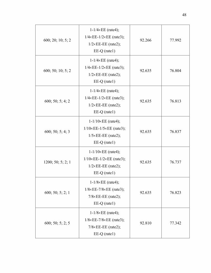
Table 2. Adjusting gradient exploration rate scheme (see Figure 17).
PARAMETERS:
explore rate (gradient)
EE; rate1; rate2; rate3; rate4
Partition of
Training Set
Classification Accuracy (%)
average of max values for each
set of tests (over 30 runs)
average over 210 program
runs
200; 20; 10; 5; 2
1-1/4×EE (rate4);
1/4×EE-1/2×EE (rate3);
1/2×EE-EE (rate2);
EE-Q (rate1)
92.266 77.887
400; 20; 10; 5; 2
1-1/4×EE (rate4);
1/4×EE-1/2×EE (rate3);
1/2×EE-EE (rate2);
EE-Q (rate1)
92.266 77.830
48
600; 20; 10; 5; 2
1-1/4×EE (rate4);
1/4×EE-1/2×EE (rate3);
1/2×EE-EE (rate2);
EE-Q (rate1)
92.266 77.992
600; 50; 10; 5; 2
1-1/4×EE (rate4);
1/4×EE-1/2×EE (rate3);
1/2×EE-EE (rate2);
EE-Q (rate1)
92.635 76.804
600; 50; 5; 4; 2
1-1/4×EE (rate4);
1/4×EE-1/2×EE (rate3);
1/2×EE-EE (rate2);
EE-Q (rate1)
92.635 76.813
600; 50; 5; 4; 3
1-1/10×EE (rate4);
1/10×EE-1/5×EE (rate3);
1/5×EE-EE (rate2);
EE-Q (rate1)
92.635 76.837
1200; 50; 5; 2; 1
1-1/10×EE (rate4);
1/10×EE-1/2×EE (rate3);
1/2×EE-EE (rate2);
EE-Q (rate1)
92.635 76.737
600; 50; 5; 2; 1
1-1/8×EE (rate4);
1/8×EE-7/8×EE (rate3);
7/8×EE-EE (rate2);
EE-Q (rate1)
92.635 76.823
600; 50; 5; 2; 5
1-1/8×EE (rate4);
1/8×EE-7/8×EE (rate3);
7/8×EE-EE (rate2);
EE-Q (rate1)
92.810 77.342
49
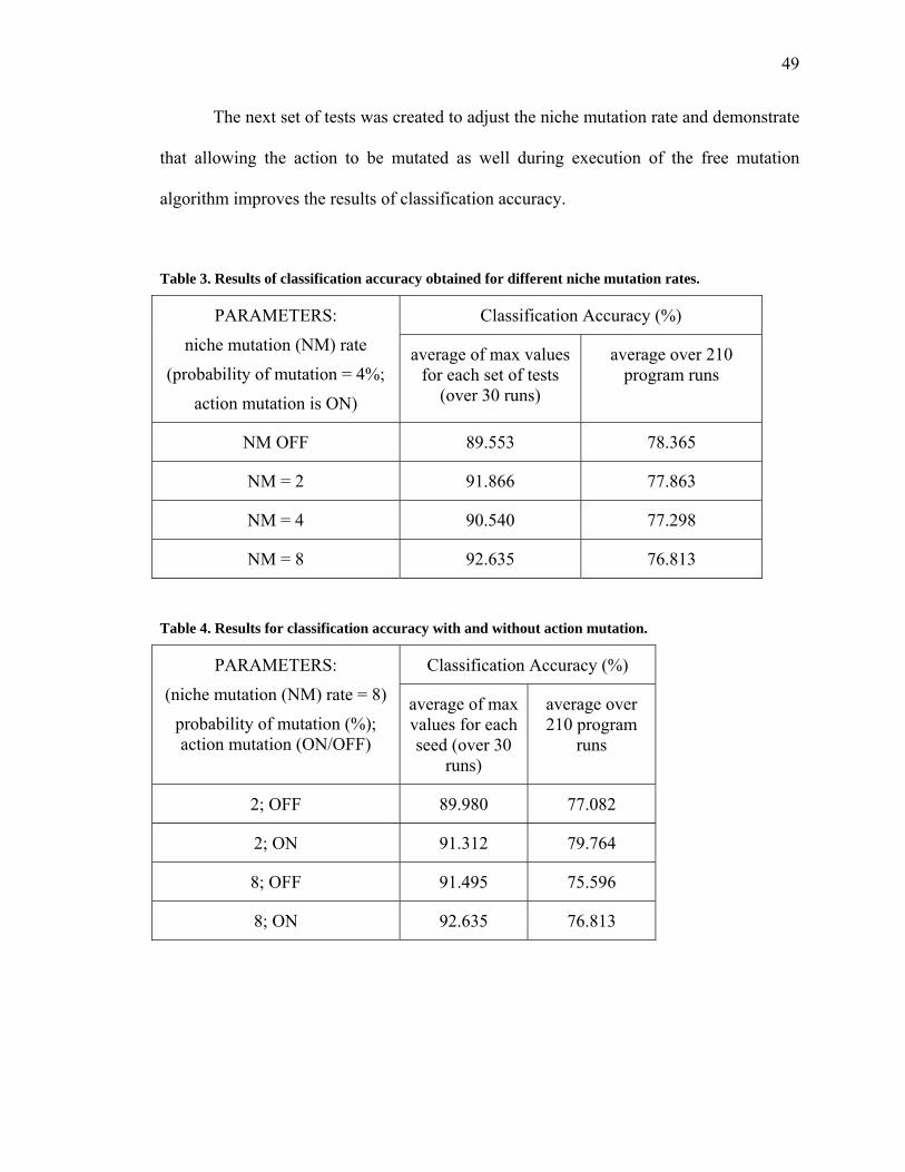
The next set of tests was created to adjust the niche mutation rate and demonstrate
that allowing the action to be mutated as well during execution of the free mutation
algorithm improves the results of classification accuracy.
Table 3. Results of classification accuracy obtained for different niche mutation rates.
PARAMETERS:
niche mutation (NM) rate
(probability of mutation = 4%;
action mutation is ON)
Classification Accuracy (%)
average of max values for each set of tests
(over 30 runs)
average over 210 program runs
NM OFF 89.553 78.365
NM = 2 91.866 77.863
NM = 4 90.540 77.298
NM = 8 92.635 76.813
Table 4. Results for classification accuracy with and without action mutation.
PARAMETERS:
(niche mutation (NM) rate = 8)
probability of mutation (%); action mutation (ON/OFF)
Classification Accuracy (%)
average of max values for each seed (over 30
runs)
average over 210 program
runs
2; OFF 89.980 77.082
2; ON 91.312 79.764
8; OFF 91.495 75.596
8; ON 92.635 76.813

50
Finally, we run a set of tests to experiment with different deletion schemes and
demonstrate an advantage of the scheme we have been using in our implementation of
XCS. Thus, Deletion Scheme 1 refers to having the probability of deletion of each
classifier be proportional to the estimate of size [A]; Deletion Scheme 2 refers to having
the probability of deletion of each classifier be as in Deletion Scheme 1 and multiplied by
the mean fitness over the current population set [P] and divided by the classifier’s fitness;
and Deletion Scheme 3 refers to the combination of the previous two that could be
adjusted using the deletion experience (DE) parameter and using a fraction of maximum
population size as an initial population of classifiers. In addition, to enhance the
advantage of the advanced deletion scheme listed above, we also implemented and used
subsumption deletion (see the description of XCS algorithm).
Table 5. Results of classification accuracy for different deletion schemes.
PARAMETERS:
Deletion Scheme;
Initial Population Size
(Deletion Experience= 15)
Classification Accuracy (%)
average of max values for each seed (over 30
runs)
average over 210 program
runs
1; 500 77.965 68.408
2; 500 79.110 68.939
3; 500 78.226 68.585
3; 300 87.048 73.101
3; 100 92.635 76.813

51
4.2 Kernel-Based Pattern Recognition Methods
After the noticeable success of Support Vector Machines (SVMs), a classification
algorithm, that was introduced in 1995 by Vapnic [65] and which performs better than
other classification algorithms in a wide range of problems, the usage of kernel methods
has been extended into other areas of machine learning and pattern recognition as well:
Kernel Fisher discriminant (KFD) [81], [82], kernel principal component analysis
(KPCA) [83], and most recently, kernel-based hard and fuzzy clustering [84], [85], [86],
[87].
The philosophy behind the versatile family of kernel methods is that the kernel
functions, or just kernels, implicitly define nonlinear transformations that map linearly
inseparable input data from the original input space Nℜ into a higher dimensional
feature space F, where the relations among the feature vectors can be represented in a
linear form, and therefore, the data can be linearly separated.
Kernels are a special type of mathematical functions with specific properties.
Each kernel )(⋅k computes the inner product of the images of the two data points in F and
can be expressed as follows:
>ΦΦ=<Φ⋅Φ= )(),()()(),( yxyxyxk rrrrrr ( 8 )
where FN →ℜΦ : performs a mapping from the original input space Nℜ into
the feature space F, such that the image of any feature vector xr in the feature space F
becomes )(xrΦ .

52
The important aspect of this kind of nonlinear mapping is that it is possible to
compute Euclidean distance in the feature F without even knowing Φ explicitly through
the distance kernel trick [67], [88]:
))()(())()((||)()(|| 2 yxyxyx rrrrrrΦ−Φ⋅Φ−Φ=Φ−Φ
)()()()(2)()( yyyxxx rrrrrrΦ⋅Φ+Φ⋅Φ−Φ⋅Φ=
),(2),(),( yxkyykxxk rrrrrr−+= ( 9 )
Examples of the mostly often-used kernels are:
Linear kernel:
yxyxk l rrrr⋅=),()( ( 10 )
Polynomial kernel of degree p:
pp yxyxk )(),()( rrrr⋅+= α , p ∈ ℕ ( 11 )
Gaussian kernel:
⎟⎟⎠
⎞⎜⎜⎝
⎛ −−= 2
2)(
2||||exp),(
σyxyxk grr
rr, σ ∈ ℝ ( 12 )
Sigmoid kernel:
))(tanh(),()( βα +⋅×= yxyxk s rrrr ( 13 )
In our work, we consistently used the Gaussian kernel, when it was applicable, as
a kernel-induced metric for measuring distances between feature vectors or a feature
vector and a center of a cluster in the feature space F. Gaussian functions have a long
history of being used in machine learning and pattern recognition and proved themselves
to be efficient and simple in computations and to be robust to noise and outliers in
classification tasks.

53
Since the Gaussian kernel functions form the hidden units of a Radial Basis
Function Network; therefore, they are often called the RBF kernels. For the Gaussian
kernel the images of all feature vectors in F have norm 1, since 1)0exp(),( ==xxk rr . The
parameter σ controls the flexibility of the kernel. As the Gaussian kernel of two points
becomes bigger, the closer those two points are in the input space.
Even though a kernel component of any kernel method is data specific, it can be
combined with different algorithms to solve a wide range of tasks. Nowadays, more and
more scientists and engineers, who are working in the different fields of machine learning
and pattern recognition, embrace a new powerful paradigm of kernel methods and tend to
view many traditional machine learning and pattern analysis algorithms from the
standpoint of this new methodology. From this viewpoint, any algorithm that uses a
kernel function to process the data and builds its discriminant function (also called a
pattern function, which is used to process unseen examples in order to classify or label
them) using kernels can be (and should be) considered as a kernel-based algorithm.
4.2.1 Radial Basis Function Neural Network (RBF NN)
Radial basis function neural networks (RBF NNs) are one of many powerful
examples of kernel methods for pattern analysis. RBF NNs have been successfully used
in a wide variety of applications and their learning and generalization abilities are well
documented [55], [56], [57], [58], [59], [89], [90]. The architecture and training
algorithms for RBF NNs are simple and their learning is considerably faster than other
forms of multilayer neural networks.
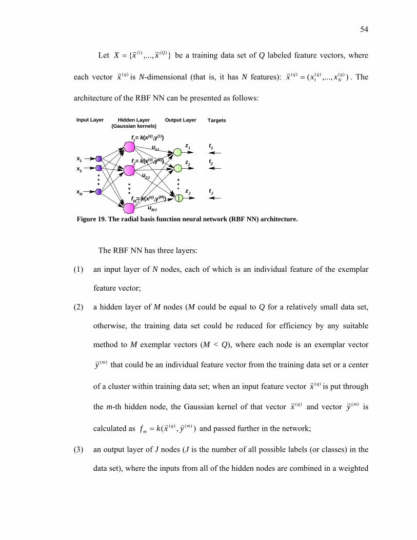
54
Let },...,{ )()1( QxxX rr= be a training data set of Q labeled feature vectors, where
each vector )(qxr is N-dimensional (that is, it has N features): ),...,( )()(1
)( qN
qq xxx =r . The
architecture of the RBF NN can be presented as follows:
The RBF NN has three layers:
(1) an input layer of N nodes, each of which is an individual feature of the exemplar
feature vector;
(2) a hidden layer of M nodes (M could be equal to Q for a relatively small data set,
otherwise, the training data set could be reduced for efficiency by any suitable
method to M exemplar vectors (M < Q), where each node is an exemplar vector
)(myr that could be an individual feature vector from the training data set or a center
of a cluster within training data set; when an input feature vector )(qxr is put through
the m-th hidden node, the Gaussian kernel of that vector )(qxr and vector )(myr is
calculated as ),( )()( mqm yxkf rr
= and passed further in the network;
(3) an output layer of J nodes (J is the number of all possible labels (or classes) in the
data set), where the inputs from all of the hidden nodes are combined in a weighted
Input Layer Hidden Layer(Gaussian kernels)
Output Layer Targets
f1= k(x(q),y(1))
f2= k(x(q),y(2))
fM= k(x(q),y(M))
z1
z2
zJ
t1
t2
tJ
u11
u2J
uMJ
x1
x2
xN
Figure 19. The radial basis function neural network (RBF NN) architecture.

55
average at each output node. The weights {umj} are the learned gains on the lines
from the hidden layer to the output layers – they get adjusted during the training
phase, so that each output will match the corresponding target (targets are the
numerical class labels).
The RBF NN is trained using the set of labeled feature vectors in the following
fashion. Each labeled feature vector Qqx q ,...,1:)( =r is fed into the network and passed
through all of hidden nodes where the Gaussian kernels are calculated:
),( )()( mqm yxkf rr
= ( 14 )
where )(myr is an m-th node exemplar feature vector and Mm ,...,1= .
The output mf is weighted by the corresponding weights (weights are initially set
to some random numbers between 0 and 1 and updated at each iteration of the training
phase) and the weighted sum is averaged over all hidden nodes at each j-th output node:
m
M
mmjj fu
Mz ∑
=
=1
1 ( 15 )
The objective of the RBF NN algorithm is to minimize the mean square error
function E by adjusting the weights {umj} so that when the training phase is completed,
the outputs should match the target vectors:
2
11
2
1)1()( m
M
mmj
J
jjj
J
jj fu
MtztE ∑∑∑
===
−=−= ( 16 )
Thus, to minimize E over all weights JjMmumj ,...,1;,...,1: == :
( ) 021
=⎟⎟⎠
⎞⎜⎜⎝
⎛−−=⎟
⎟⎠
⎞⎜⎜⎝
⎛
∂
∂⎟⎟⎠
⎞⎜⎜⎝
⎛
∂∂
=∂∂ ∑
= Mf
ztuz
zE
uE m
J
jjj
mj
j
jmj
( 17 )

56
Using the steepest descent method, we can update the weights for each feature
vector:
)()()1(
kmj
kmj
kmj u
Euu∂∂
−=+
( ) m
J
jjj
kmj fzt
Mu ⎟⎟
⎠
⎞⎜⎜⎝
⎛−+= ∑
=1
)( 2η ( 18 )
where η is a learning rate (or step size).
Upon training the RBF NN over all Q labeled feature vectors from the training
data set, each new weight umj is calculated as follows:
( )∑ ∑= =
+⎟⎟⎠
⎞⎜⎜⎝
⎛−+=
Q
q
qm
J
j
qj
qj
kmj
kmj fzt
Muu
1
)(
1
)()()()1( 2η
( )∑ ∑= =
⎟⎟⎠
⎞⎜⎜⎝
⎛−+=
Q
q
J
j
qj
qj
mqkmj ztyxk
MJQu
1 1
)()()()()( ),(2 rrη ( 19 )
After implementing the RBF NN algorithm, it was tested by using the benchmark
data set (the Wisconsin breast cancer data set). We used the reduced training set of
feature vectors for the hidden nodes – we eliminated those feature vectors that were too
close to others by using the fraction of the average distance between all pairs of vectors in
the data set, the remaining vectors were used to form Gaussian kernels. After the network
was trained, the testing data set was used to asset the quality of the RBF NN:
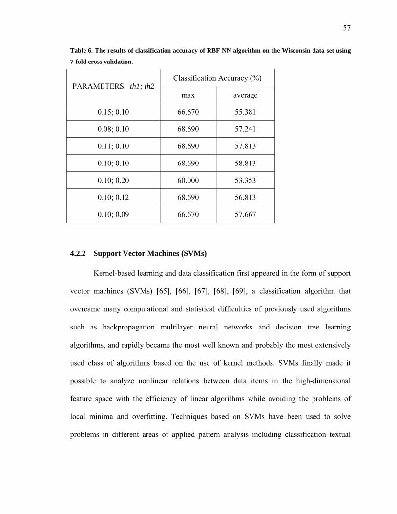
57
Table 6. The results of classification accuracy of RBF NN algorithm on the Wisconsin data set using
7-fold cross validation.
PARAMETERS: th1; th2 Classification Accuracy (%)
max average
0.15; 0.10 66.670 55.381
0.08; 0.10 68.690 57.241
0.11; 0.10 68.690 57.813
0.10; 0.10 68.690 58.813
0.10; 0.20 60.000 53.353
0.10; 0.12 68.690 56.813
0.10; 0.09 66.670 57.667
4.2.2 Support Vector Machines (SVMs)
Kernel-based learning and data classification first appeared in the form of support
vector machines (SVMs) [65], [66], [67], [68], [69], a classification algorithm that
overcame many computational and statistical difficulties of previously used algorithms
such as backpropagation multilayer neural networks and decision tree learning
algorithms, and rapidly became the most well known and probably the most extensively
used class of algorithms based on the use of kernel methods. SVMs finally made it
possible to analyze nonlinear relations between data items in the high-dimensional
feature space with the efficiency of linear algorithms while avoiding the problems of
local minima and overfitting. Techniques based on SVMs have been used to solve
problems in different areas of applied pattern analysis including classification textual

58
documents into a number of predefined categories [91] and handwritten character
recognition [92], [93], computer vision [94], [95], bioinformatics [96], [97], and many
others [98] , [99].
One of the objectives of this thesis was to compare the performance of the several
different types of classifiers in order to find the best possible algorithm for this type of
task. One of the characteristics that made our pattern recognition task special was the
high dimensionality of the feature vectors and a quite limited set of vectors for training. If
X is a set of Q exemplar feature vectors },...,1:{ )( Qqx q =r , where each vector has N
features, ),...,,( )()(2
)(1
)( qN
qqq xxxx =r , then Q << N in the case of our classification problem.
Scientific research conducted in the area of pattern recognition that deals with
highly dimensional vector spaces and limited numbers of exemplar vectors in the data
sets, suggests that one of the best performers for this type of classification tasks is a
Support Vector Machine algorithm.
Support Vector Machines (SVMs) are learning systems that “use a hypothesis
space of linear functions in a high dimensional feature space, trained with a learning
algorithm from optimization theory that implements a learning bias derived from
statistical learning theory” [66]. The theory behind SVMs has a quite complex, but at the
same time, well defined mathematical model that is built on rigorous theoretical analyses
and therefore, guarantees computational efficiency. It is mostly based on statistical
learning theory, notions of high dimensional vector spaces, support vectors, and kernel
functions that can map vectors from one vector space to another. SVMs rely on
preprocessing the data to represent patterns in a high dimensional space by mapping them

59
using the some transformation function )(xrΦ , which we don’t have to know explicitly.
As in the case of all kernel methods, instead of computing the mapping function )(xrΦ
explicitly, the SVMs algorithm replaces it with the kernel function
)()(),( )()( ii sxsxk rrrrΦ⋅Φ= , where )(isr is an i-th support vector, and uses it for training.
Typically, the new vector space where the data become linearly separable is much
higher dimensional than the original input vector space. With an appropriate nonlinear
mapping to a sufficiently high dimensional vector space, data from two (or more)
different categories can always be separated by a hyperplane (or several hyperplanes in
the case of multiclass environment). The objective of the SVM classifier is to create a
separating hyperplane with the largest possible margin. The larger the margin is, the
better the generalization of the created classifier. The margin is normally determined by
support vectors (Figure 20). The support vectors are the exemplar vectors from the
training data set that are the closest to the hyperplane. These vectors define the optimal
separating hyperplane and are the most difficult patterns to classify. In the SVM
algorithm, the support vectors are the most important and informative vectors for the
classification purpose. Normally, after determining support vectors, the algorithm ignores
all the rest of the training set. This is one of the reasons for the computational efficiency
of SVMs.
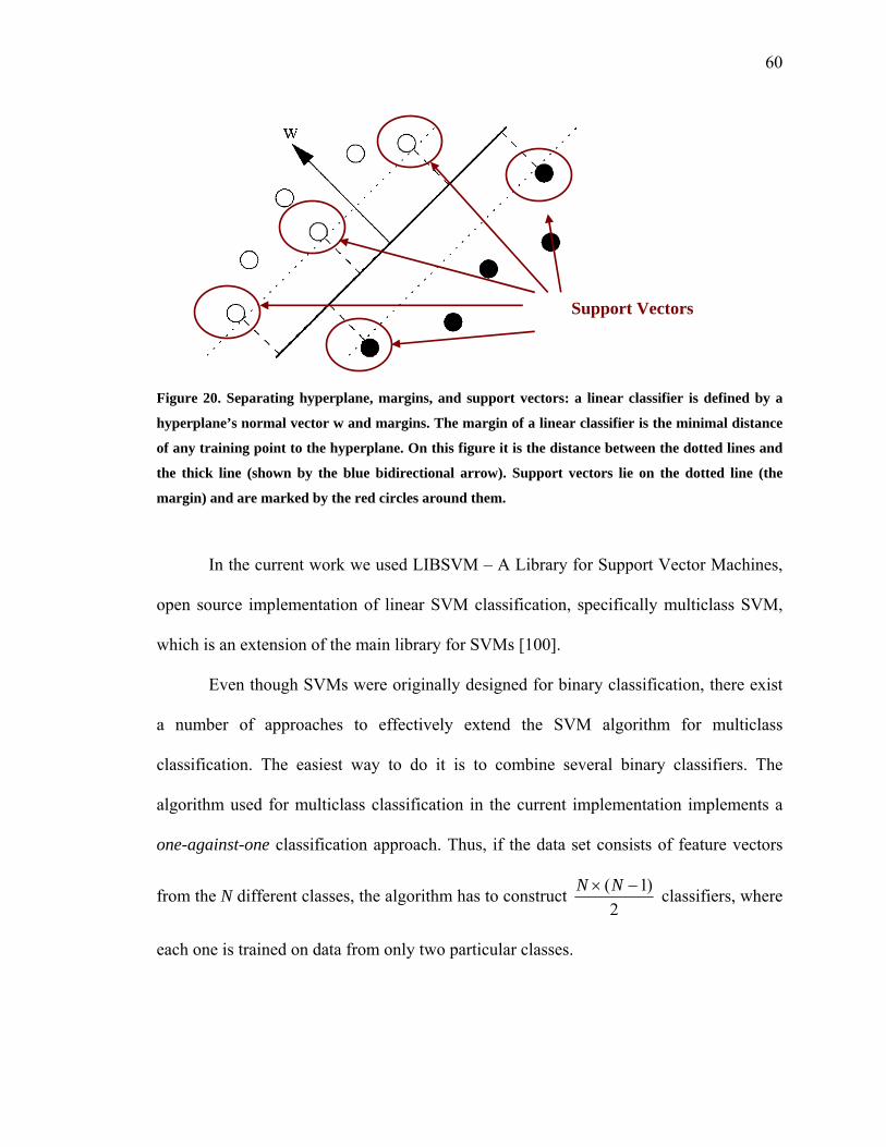
60
Figure 20. Separating hyperplane, margins, and support vectors: a linear classifier is defined by a
hyperplane’s normal vector w and margins. The margin of a linear classifier is the minimal distance
of any training point to the hyperplane. On this figure it is the distance between the dotted lines and
the thick line (shown by the blue bidirectional arrow). Support vectors lie on the dotted line (the
margin) and are marked by the red circles around them.
In the current work we used LIBSVM – A Library for Support Vector Machines,
open source implementation of linear SVM classification, specifically multiclass SVM,
which is an extension of the main library for SVMs [100].
Even though SVMs were originally designed for binary classification, there exist
a number of approaches to effectively extend the SVM algorithm for multiclass
classification. The easiest way to do it is to combine several binary classifiers. The
algorithm used for multiclass classification in the current implementation implements a
one-against-one classification approach. Thus, if the data set consists of feature vectors
from the N different classes, the algorithm has to construct 2
)1( −× NN classifiers, where
each one is trained on data from only two particular classes.
Support Vectors

61
After all binary classifiers have been constructed the way to use them for the
future testing may not be so obvious. There exist some methods for doing so, and the one
that the LIBSVM implementation uses is based on a voting strategy. If during testing the
algorithm has to decide for the unlabeled feature vector xr between class i and class j and
the discriminant function suggests that xr is in i-th class, then the vote for class i is added
by one, otherwise, the vote added for class j. After all classifiers have been tested, the
class with the largest number of votes wins and xr gets that class’ label.
Again, we used the Wisconsin breast cancer data set as a benchmark data set to
test the SVM algorithm in order to compare the results of classification with all pattern
recognition algorithms developed before within the framework of the current research.
Table 7. The results of classification accuracy of SVM algorithm on the Wisconsin data set using
7-fold cross validation.
Type of kernel Classification Accuracy (%)
max average
Linear: )()()( ),( iil sxsxk rrrr⋅= 100.000 95.997
Polynomial: 3)()()( )(),( iip sxsxk rrrr⋅= 97.980 90.140
Polynomial: 3)()()( )1(),( iip sxsxk rrrr⋅+= 100.000 96.284
Gaussian: ⎟⎟⎠
⎞⎜⎜⎝
⎛ −−=
9||||exp),(
2)()()(
iig sxsxk
rrrr 100.000 96.284
Sigmoid: ))(91tanh(),( )()()( iis sxsxk rrrr
⋅×= 85.860 75.266
Sigmoid: )1)(91tanh(),( )()()( +⋅×= iis sxsxk rrrr 78.790 65.541
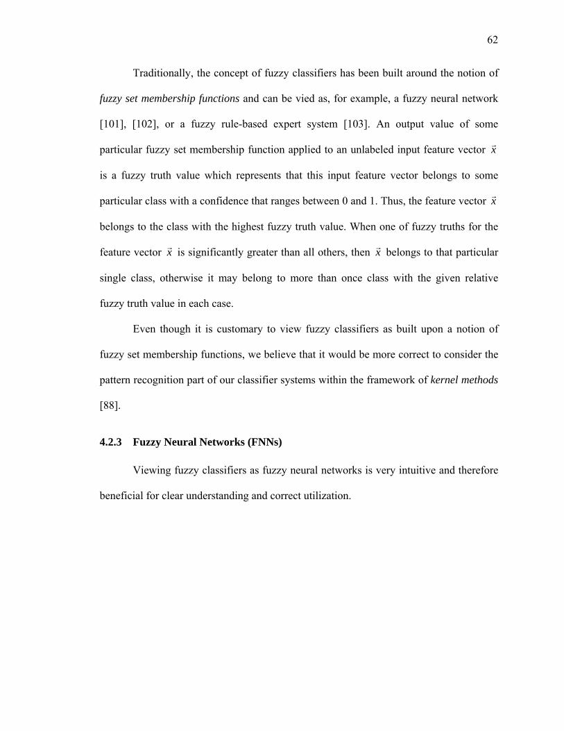
62
Traditionally, the concept of fuzzy classifiers has been built around the notion of
fuzzy set membership functions and can be vied as, for example, a fuzzy neural network
[101], [102], or a fuzzy rule-based expert system [103]. An output value of some
particular fuzzy set membership function applied to an unlabeled input feature vector xr
is a fuzzy truth value which represents that this input feature vector belongs to some
particular class with a confidence that ranges between 0 and 1. Thus, the feature vector xr
belongs to the class with the highest fuzzy truth value. When one of fuzzy truths for the
feature vector xr is significantly greater than all others, then xr belongs to that particular
single class, otherwise it may belong to more than once class with the given relative
fuzzy truth value in each case.
Even though it is customary to view fuzzy classifiers as built upon a notion of
fuzzy set membership functions, we believe that it would be more correct to consider the
pattern recognition part of our classifier systems within the framework of kernel methods
[88].
4.2.3 Fuzzy Neural Networks (FNNs)
Viewing fuzzy classifiers as fuzzy neural networks is very intuitive and therefore
beneficial for clear understanding and correct utilization.
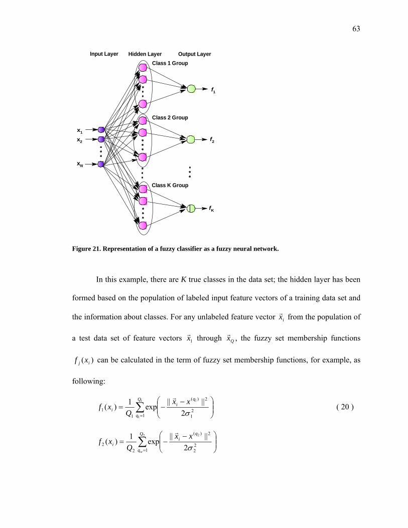
63
Input Layer Hidden Layer Output Layer
f1
x1
x2
xN
f2
fK
Class 1 Group
Class 2 Group
Class K Group
Figure 21. Representation of a fuzzy classifier as a fuzzy neural network.
In this example, there are K true classes in the data set; the hidden layer has been
formed based on the population of labeled input feature vectors of a training data set and
the information about classes. For any unlabeled feature vector ixr from the population of
a test data set of feature vectors 1xr through Qxr , the fuzzy set membership functions
)( ij xf can be calculated in the term of fuzzy set membership functions, for example, as
following:
∑=
⎟⎟⎠
⎞⎜⎜⎝
⎛ −−=
1
1
1
121
2)(
11 2
||||exp1)(
Q
q
qi
ixx
Qxf
σ
r
( 20 )
∑=
⎟⎟⎠
⎞⎜⎜⎝
⎛ −−=
2 2
122
2)(
22 2
||||exp1)(
Q
q
qi
iw
xxQ
xfσ
r

64
: :
∑=
⎟⎟⎠
⎞⎜⎜⎝
⎛ −−=
2
12
2)(
2||||
exp1)(Q
q K
qi
KiK
K
KxxQ
xfσ
r
where Q1, Q2,…, QK are the number of feature vectors in class 1, class 2, … class
K respectively; )( jqxr is q-th feature vector of class j.
Fuzzy Neural Networks (FNNs) are the simplest class of fuzzy classifier systems:
their nodes do not have weights and they do not require extensive training. Since we
constructed our FNN within framework of the kernel methods, we consider our classifier
to be based on “kernelization” of the metric for measuring distances between the centers
of clusters that were established in the input space and the unlabeled feature vectors, as
was shown before (Eq. 9):
),(2),(),(||)()(|| )()()(2)( jjjj qqqq xxkxxkxxkxx rrrrrrrr−+=Φ−Φ ( 21 )
where xr is an arbitrary unlabeled feature vector from the test data set and )( jqxr is
a q-th feature vector of class j in the training data set. Since ),( xxk rr and ),( )()( jj qq xxk rr are
both constants (and equal to 1) then, in order to find the closest labeled feature vector to
the given unlabeled feature vector, we should look for the greatest value of the kernel – in
our case the Gaussian kernel (Eq. 12):
⎟⎟⎠
⎞⎜⎜⎝
⎛ −−= 2
2)()()(
2||||exp),(
j
qqg
jj xxxxk
σ
rrrr
( 22 )
where jσ is a variance of the j-th class in the training data set. If the data of the
given class has been proven not to contain outliers (feature vectors that are numerically
distant from the rest of the data) or mislabeled feature vectors, the variance can be

65
computed as a fraction (between 31 and
21 ) of the average distance between every two
labeled feature vector within class j.
We tried two different approaches in constructing our fuzzy classifier.
In the first approach, we construct a discriminant function as the maximum kernel
value for the unlabeled feature vector xr and every labeled feature vector within each
class:
},...,1:),({max{)( )(1jj
qj Qqxxkxf j ==
rrr ( 23 )
where )(1 xf jr is the first constructed discriminant function for unlabeled feature
vector xr over class j; ),( )( jqxxk rr is a Gaussian kernel as in (Eq. 12); )( jqxr is a q-th
feature vector of class j in the training data set, jj Qq ,...,1= ; and Qj is the total number of
feature vector in class j.
In the second approach, instead of using the maximum kernel values for an
individual feature vector over each class, the algorithm uses the average value of all
possible kernel values in each class:
∑=
=j
j
j
Q
q
q
jj xxk
Qxf
1
)(2 ),(1)( rrr ( 24 )
where )(2 xf jr is the second constructed discriminant function for unlabeled
feature vector xr over class j and everything else is as above.
After evaluating the discriminant functions for all classes, the labeling procedure
is straightforward: the unlabeled vector xr from the test set belongs to the class for which
the discriminant function has the largest value.
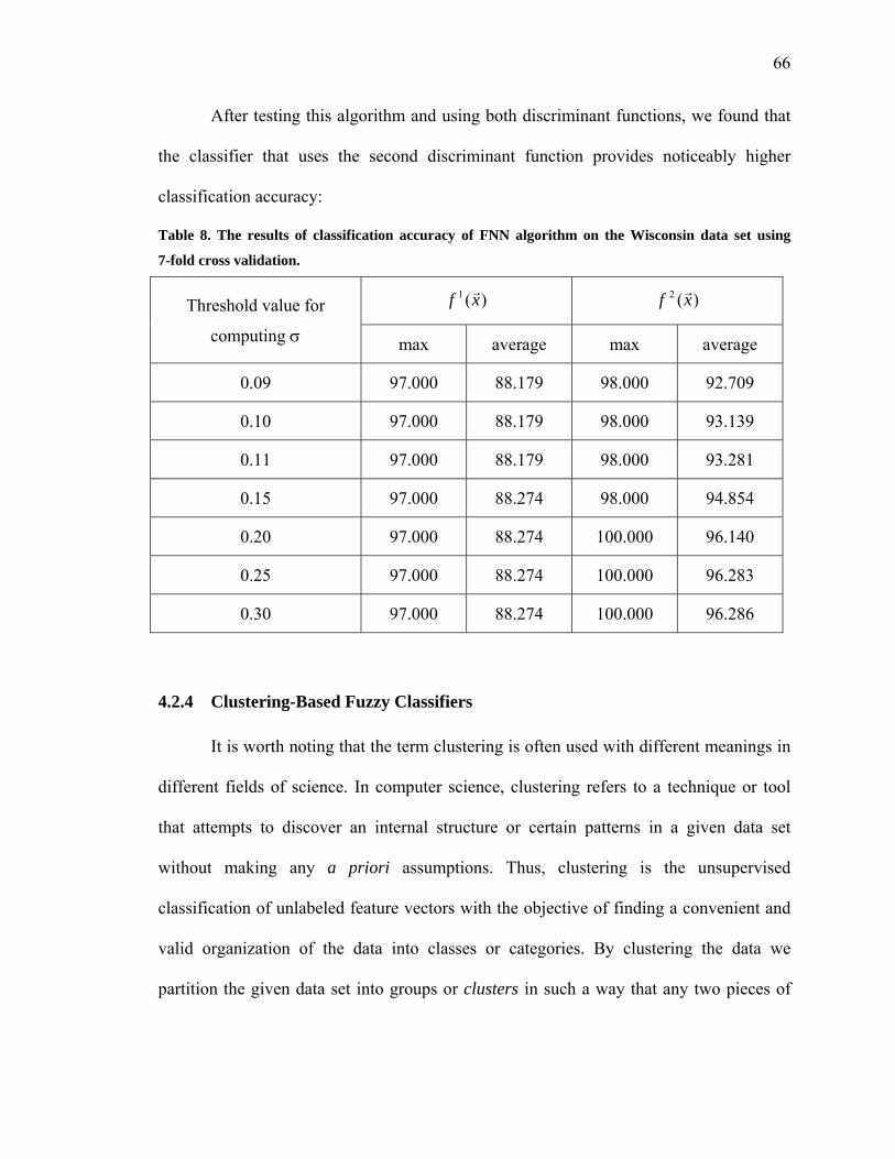
66
After testing this algorithm and using both discriminant functions, we found that
the classifier that uses the second discriminant function provides noticeably higher
classification accuracy:
Table 8. The results of classification accuracy of FNN algorithm on the Wisconsin data set using
7-fold cross validation.
Threshold value for
computing σ
)(1 xf r )(2 xf r
max average max average
0.09 97.000 88.179 98.000 92.709
0.10 97.000 88.179 98.000 93.139
0.11 97.000 88.179 98.000 93.281
0.15 97.000 88.274 98.000 94.854
0.20 97.000 88.274 100.000 96.140
0.25 97.000 88.274 100.000 96.283
0.30 97.000 88.274 100.000 96.286
4.2.4 Clustering-Based Fuzzy Classifiers
It is worth noting that the term clustering is often used with different meanings in
different fields of science. In computer science, clustering refers to a technique or tool
that attempts to discover an internal structure or certain patterns in a given data set
without making any a priori assumptions. Thus, clustering is the unsupervised
classification of unlabeled feature vectors with the objective of finding a convenient and
valid organization of the data into classes or categories. By clustering the data we
partition the given data set into groups or clusters in such a way that any two pieces of
67
data from the same cluster are as similar as possible and any two pieces of data from
different clusters as dissimilar as possible.
Although traditionally clustering deals with unlabeled data, which are data items
that contain no class information attached to them, and is considered a method of
unsupervised learning, clustering is very useful in implementing a “divide and conquer”
strategy to reduce the computational complexity of various decision-making algorithms
in pattern recognition. For example, initial clustering of the data is widely used in popular
techniques in pattern recognition such as the nearest-neighbor decision rule [104] or for
problem localization [105].
In our case, class information for a training set of feature vectors is available. It
might seem that the use of unsupervised learning methods, such as clustering, is not
necessary. However, we have found that having established the internal structure in our
data set first through clustering the data helps us tremendously in finding the rules for
assigning the unlabeled data items to correct classes. Data could be noisy, contain outliers
or missing features, or could be labeled incorrectly. Cluster analysis, as the most
prominent example of unsupervised learning, is very good at dealing with all these and
many other similar cases.
The experimental data we collected during our experiments with chemical vapors
were sometimes slightly, sometimes noticeably different from day to day. This effect
happened even though all formal experimental conditions (such as the concentration of
chemical vapors in the gaseous mixture, the temperature of the array cell, etc.) were the
same. This was mostly due to the fact that some parameters of our experimental setup and
some experimental conditions could not be reproduced precisely or controlled completely
68
each time. One such parameter is the low precision of the settings of the device that
creates the desirable concentration of chemical vapors in the gaseous mixture. The
imprecision in that device’s settings resulted in sometimes considerably different real
concentrations of chemical vapors created from one experiment to another. Thus, it
would be quite difficult to “explain” to our algorithm how sometimes quite different
feature vectors (that were created from the data collected on different days) can belong to
the same class. We thought that unsupervised learning such as fuzzy clustering in our
case might actually help us with this problem. The algorithm would naturally partition
training vectors from the same class into several different clusters (if the necessity arises)
and increase the chances of correct classification of the unseen exemplar vectors.
For both our fuzzy clustering algorithms, we performed a pre-clustering
procedure, whose goal is reducing the data set for efficiency. Pre-clusters are the result of
preliminary partitioning of the data set and they can be considered as some sort of proto-
clusters. Pre-clusters are typically very compact and have a hyperspherical shape. We
used an improved k-means clustering algorithm for this purpose.
4.2.4.1 Pre-clustering by Improved K-Means Clustering
The k-means algorithm is one of the most popular clustering methods − it is very
simple, straightforward, and robust; therefore, it has been used in a wide spectrum of
applications [106]. This algorithm employs the most intuitive and frequently used
criterion function in partitional clustering – the squared error criterion:
2)(
1 1
)()()1( ||||}),...,({ jK
j
Q
i
iK cxCCFj
j rr∑∑= =
−= ( 25 )
69
where K is the number of clusters in the data set; )()1( ,..., KCC are K clusters that
the data set has been partitioned into; Qj is the number of feature vectors in each cluster;
)( jixr is the ith feature vector belonging to the jth cluster, )( jC ; and )( jcr is the center of the
cluster )( jC .
The k-means algorithm works as following:
(1) Select the initial K cluster centers randomly over the input domain.
(2) Assign each feature vector to its closest cluster center and compute the new cluster
centers as cluster prototypes. Repeat this step until convergence is achieved, e.g.,
there is no reassignment of any feature vector from one cluster to another, or the
criterion function doesn’t change noticeably anymore.
(3) Merge and split clusters based on some heuristic information, optionally repeating
step (2).
As can be deducted from the above algorithm description, the traditional k-means
algorithm requires a priori knowledge about the number K of clusters in the data set,
which often is unknown beforehand, and can suffer from bad or unfortunate initial cluster
centers selection [107]. We looked for improvements of the k-means algorithm similar to
those described in [108] and [109] that would significantly reduce the algorithm’s
drawbacks. Since we didn’t have to deal with guessing the number of possible classes in
the data set or handling problems that large data sets normally bring with them, our task
became significantly easier than the typical case of partitioning of unknown data set
within framework of unsupervised learning.

70
After a number of experimentations, we developed two modifications of the
improved k-means algorithm. The first modification was for establishing the initial pre-
clusters in the Fuzzy C-Means (FCM) clustering algorithm:
Calculate the test threshold as a fraction of an average distance between all
possible pairs of feature vectors in the initial data set.
Instead of starting with K random initial points as cluster centers or an empty set
of centers, start with the maximally possible number of centers, Q, where Q is the number
of all feature vectors in the set. Next, eliminate the feature vectors that are too close to
other centers from the set of possible cluster centers using the threshold value and assign
the eliminated feature vector to the closest center.
On each iteration, the feature vectors that were eliminated from the set of centers
are checked once again against the new center that is under examination: if the distance
from some vector that was assigned to another center before to current center is less than
the distance to its previous center, reassign this point to the current center. This newly
added modification to the clustering procedure is very important as it eliminates the
dependency of the clustering procedure on the order of instantiating the initial cluster
centers and merging feature vectors in the pre-clusters.
After the tentative number of initial cluster centers has been established, the
algorithm calculates the number of vectors in each cluster. The clusters that contain a
smaller number of vectors than was specified by a programmer or user are eliminated as
well. The vectors from those clusters are assigned to the nearest neighboring clusters.
From this point, the algorithm continues clustering using an improved k-means clustering
algorithm: at each iteration, it keeps recalculating the cluster centers, reassigning all

71
vectors to the newly created cluster centers, and eliminating those clusters that contain
fewer vectors than a given threshold. The algorithm repeats this processing until the set
of the cluster centers remains unchanged.
For our second fuzzy clustering algorithm, fuzzy connectivity clustering, we made
further modification into the improved k-means algorithm, since we had more flexibility
in preprocessing the training data.
First, we wanted to automate the adjustment of the number of pre-clusters and
make it independent from the user pre-settings. For this purpose, we chose the permitted
range for the number of initial pre-clusters in the data set first. The number of preliminary
clusters (or pre-clusters) should correlate with the number of true classes, which is known
in our case. We normally use the range: NKN ×≤≤× 152 , where N is the number of
true classes and K is the final number of pre-clusters.
Initially, the algorithm calculates the test threshold as a fraction of an average
distance between all possible pairs of feature vectors in the data set. After that, it
automatically adjusts the threshold value for eliminating centers based on their proximity
to other centers so that the final number of pre-clusters fits into the given range; that is, if
the number of pre-clusters are greater than the maximum number in the specified range,
the program increases the threshold value by the specified learning rate, if the number of
pre-clusters are less than the minimum number in the specified range, it decreases the
threshold value by the specified learning rate.
Second, we now allow having single-point clusters, which are typically outliers.
Thus, we do not enforce any rule in this modification of the improved k-means algorithm

72
such as that each cluster has to have at least a few feature vectors as we did before
(normally, this number is five or more).
Using this particular modification of the improved k-means algorithm we do not
have to worry about the outliers; therefore, we do not have to calculate the trimmed mean
of each pre-cluster, since the embedded requirement to the pre-clusters to be compact
excludes the possibility of outliers to be included in any of them.
After the desirable number of pre-clusters has been established, the program
calculates the means of all pre-clusters and uses those means as a final set of cluster
centers. Typically, each resulting cluster contains several pre-clusters. This permits
resulting clusters to take their own natural shape, which is not necessarily hyperspherical.
4.2.4.2 Fuzzy Clustering
Since fuzzy models for pattern recognition became popular among scientists,
engineers, and statisticians in trying to reflect vagueness and imprecision of boundaries
between group of objects in real applications, numerous fuzzy clustering algorithms,
whose aim is to model fuzzy, i.e., ambiguous and vague, unsupervised patterns efficiently
have emerged [62], [63], [64]. In classical or crisp clustering analysis, any piece of data,
i.e., feature vector, can be assigned to only one cluster. Fuzzy clustering has removed that
constraint – it allows each feature vector in the data set to belong to more than one cluster
with different membership degrees (between 0 and 1) and vague or fuzzy boundaries
between clusters. Thus, fuzzy clustering offers an opportunity to deal with real-life data
that belong to more than one group, or class, at the same time; as for the feature vector

73
membership degree – it provides a measure of degree to which the given feature vector
fits within a particular class.
Both our fuzzy clustering algorithms take the following input files:
data files – there are two files, one contains the training data set, the other
contains the testing data set; each file contains the dimension of the feature
vectors, the number of vectors in the current data set and vectors themselves (as a
table of row vectors). The last field of each vector is a numerical representation of
the class that the given vector belongs to;
description file – the file contains the full description of all classes presented in
the training set, including the numerical class label used in the data sets.
In the training phase, the program reads in the training and testing data sets and
the description of the classes used for training. We assume that the testing data set
contains samples from the same pool of classes, i.e. there are no feature vectors in the
testing set that belong to the classes that are not present in the training data set
In the next step, the program preprocesses training set into pre-clusters using the
improved k-means algorithm described above. After the set of pre-clusters has been
established by mean of the improved k-means algorithm, our algorithm continues
clustering using the standard FCM algorithm with some minor modifications or the fuzzy
connectivity clustering algorithm (FCC).
4.2.4.3 Fuzzy Classifier based on Fuzzy C-Means Clustering (FCM-based)
Bezdek developed a family of clustering algorithms, based on a fuzzy extension
of the least-squared error criterion [62], [110]. The FCM algorithm is one of them – it is a

74
set-partitioning method based on Picard iteration through necessary conditions for
optimizing a weighted sum of squared errors objective function Jm (Eq. 26) [111].
If },...,,{ 21 QxxxX rrr= is a finite set of feature vectors in N-dimensional Euclidean
space Nℜ , then the goal of the FCM algorithm is to partition this set into C clusters
represented as fuzzy sets )()2()1( ,...,, CFFF by minimizing the objective function Jm(U, V)
with respect to U, a fuzzy C-partition of the data set, and to V, a set of C cluster
prototypes (a cluster prototype is a vector that represents its cluster; in our case it is just a
center of a given cluster):
),(),( )()(2
1 1
ikQ
k
C
i
mikm vxduVUJ rr∑∑
= =
= ( 26 )
In (Eq. 26) m is any real number greater than 1 (this is weighting exponent for
iku , or fuzzifier), the value that controls the “fuzziness”, in other words, how much
clusters may overlap. This parameter reduces the sensitivity of the cluster centers to noise
in the data). Variable )(kxr is the k-th N-dimensional feature vector, )(ivr is the prototype
(a center) of the i-th cluster, iku is the degree of membership of kx in the i-th cluster,
),( )()(2 ik vxd rr is an inner product metric (distance between vector kx and cluster center
iv ), Q is the number of feature vectors, and C is the resulting number of clusters.
The computation of the degree of membership iku depends on the definition of the
distance measure, ),( )()(2 ik vxd rr :
)()(),( )()(1)()()()(2 ikTikik vxvxvxd rrrrrr−Σ−= − ( 27 )
where Σ is an arbitrary covariance matrix.

75
In the current work we assume that the shape of all clusters is hyperspherical, so
the covariance matrix in our case is equal to the identity matrix I. Thus, the distance
),( )()(2 ik vxd rr in our case is Euclidean, as was described in the beginning of the current
chapter (Eq. 1):
( ) 2)()(
0
2)()()()(2 ||||),( ikN
i
ii
ki
ik vxvxvxd rrrr−=−= ∑
=
( 28 )
where N is the dimension of the feature vectors.
Typically, the FCM algorithm starts by choosing the number of clusters C and the
value of fuzzifier m (both parameters are chosen by a user), and by randomly initializing
the membership degree matrix U under the constraint such that 11
=∑=
C
iiku (the sum of
memberships for each feature vector over all clusters should be equal to 1). Next, the
initial cluster prototypes are computed, using the following formula:
∑
∑
=
== N
k
mik
N
kk
mik
i
u
xuv
1
1)(
)(
)(r
( 29 )
Following this step, using the computed cluster prototypes, the fuzzy
memberships iku are updated according to the equation:
∑=
−
−
⎟⎟⎠
⎞⎜⎜⎝
⎛
⎟⎟⎠
⎞⎜⎜⎝
⎛
=c
i
m
ik
m
ik
ik
vxd
vxdu
1
11
)()(2
11
)()(2
),(1
),(1
rr
rr
( 30 )

76
Next, the algorithm iterates between (Eq. 29) and (Eq. 30) until the memberships
or cluster centers for successive iteration differ by less than some termination criterion,ε ,
chosen by a programmer or user.
It is quite obvious that the standard FCM algorithm, similarly to the standard
k-means algorithm described before, is very sensitive to the initial choice of cluster
centers. Different choices of cluster prototypes may lead to convergence to different local
optima, in other words, to different partitions. In many practical situations a priori
knowledge of the approximate locations of the initial centers does not exist, and in order
to achieve optimal partition unsupervised tracking of classification prototypes is required.
That is why making a preliminary assessment of the data set structure provides
invaluable advantages over the standard approach. Thus, we used the pre-cluster centers
obtained by running the improved k-means algorithm as a starting point for the modified
FCM algorithm. Therefore, we did not have to guess the fuzzy memberships iku : we
started the main loop of the FCM algorithm by calculating those memberships (Eq. 30).
After the algorithm converges, class labels have to be assigned to each feature
vector. The quality of clustering is indicated by how closely the feature vectors are
associated to the cluster centers, and the level of association or classification is measured
by the membership functions. If the value of one of the memberships is significantly
larger than the others’ for a particular data point, then that data point is identified as being
a part of the subset of the data represented by the corresponding cluster center. Thus,
larger membership values indicate higher confidence in the assignment of the feature
vector to the particular cluster.

77
We said before that the goal of the FCM algorithm is to partition some arbitrary
set X = {x1, x2, …, xQ} into C clusters (subgroups) represented as fuzzy sets
)()2()1( ,...,, CFFF . Generally speaking, in fuzzy clustering each cluster (each fuzzy set
)(iF , Ci ≤≤1 ) is a fuzzy set of all feature vectors, that is each )(iF includes all data
points but with different values of fuzzy membership.
In the current research, our goal was to assign class labels to each data point as
one does in hard clustering, meaning that at the end, each data point should belong to one
and only one class (but probably, with different level of confidence). Thus, in our study,
fuzzy clustering was only an auxiliary tool for reaching the ultimate goal – to discover
structures or certain groupings in a data set and therefore a set of rules that significantly
facilitate the process of correct labeling of newly encountered, unseen before unlabeled
feature vectors.
Consequently, after the FCM algorithm converges (in our case, when either
memberships or cluster centers for successive iteration differ by less than the termination
criterion ε = 0.00001), the algorithm performs “hard” partitioning, meaning that at the
end each feature vector would belong to one and only one cluster, that is, to the cluster
whose membership function for this vector is the largest. At this point, the algorithm
labels the finally created clusters according to the “description file” and calculates some
statistics. It might happen that some clusters contain vectors from the different classes. If
that is the case, the algorithm calculates its confidence in class labeling according to the
percentage of the vectors from the major class in that cluster.
At this point the algorithm enters a pattern recognition phase. After the labeled
feature vectors have been clustered and each cluster was labeled as described above, we

78
constructed the fuzzy classifier over it. Again, we consider the fuzzy classifier within
framework of kernel methods, but this time it was built around clusters that the training
data set was partitioned into. And as in the case of FNN, we tried two different
approaches for designing a fuzzy classifier.
In the first approach, for each unlabeled feature vector xr the algorithm calculates
the value of a Gaussian kernel of this feature vector and each center of all clusters. In
order to assign a given feature vector to one of those clusters, we have to evaluate a
discriminant function )(xf jr , which is in this case just a Gaussian kernel with jσ being
the variance of the j-th cluster, for all C final clusters ( Cj ,...,1= ):
),()( )(1 jj vxkxf rrr
= ( 31 )
where )(1 xf jr is a discriminant function of type 1 for unlabeled feature vector xr
over cluster j; )( jvr is a center of the j-th cluster; ),( )( jvxk rr is a Gaussian kernel. The
cluster that has the largest discriminant function value is considered to be the winner, and
the unlabeled feature vector is get assigned to this cluster.
In the second approach, instead of using only the centers of the clusters, the
discriminant function is constructed to be equal to the maximum kernel value in each
cluster:
},...,1:),(max{)( )(2jj
qj Qqxxkxf j ==
rrr ( 32 )
where )(2 xf jr is a discriminant function of type 2 for unlabeled feature vector xr
over cluster j; )( jqx is a feature vectors that belongs to the j-th cluster, j = 1,…,C,
jj Qq ,...,1= ; Qj is the total number of feature vector in the j-th cluster; and ),( )( jqxxk rr is

79
a Gaussian kernel, calculated for the unlabeled feature vector xr and the q-th feature
vector of the j-th luster. As in the previous case, the unlabeled feature vector xr gets
assigned to the cluster that has the largest value of the discriminant function )(2 xf jr .
After the unlabeled feature vector has been assigned to some cluster, it also gets a
label from the cluster. If the “winning” cluster has high confidence in its label, i.e. the
absolute majority of the vectors in that cluster belong to the same class, we have high
confidence in the performed classification. Otherwise, our confidence might be as low as
the percentage of the major class in the given cluster (e.g., 80%, or even 70%, but this is
rarely the case).
After testing the current algorithm by using the benchmark data set (the
Wisconsin breast cancer data set), we found that the classifier based on the discriminant
function of type 2 gives higher accuracy of classification.
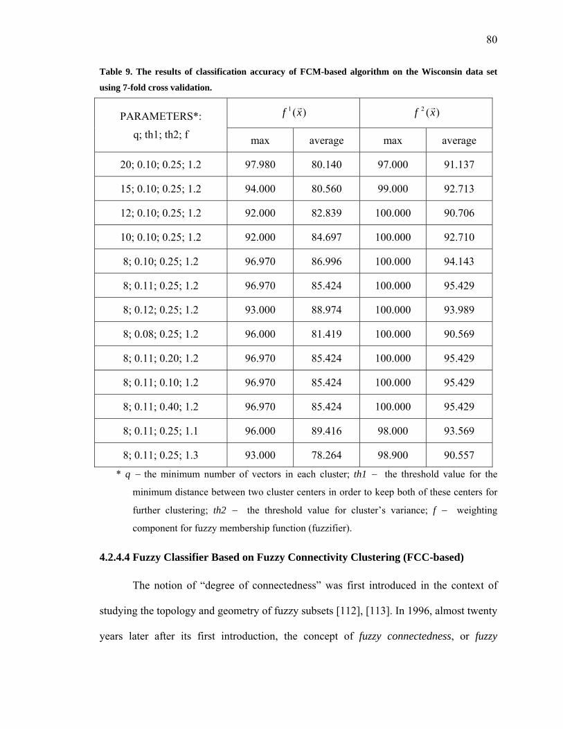
80
Table 9. The results of classification accuracy of FCM-based algorithm on the Wisconsin data set
using 7-fold cross validation.
PARAMETERS*:
q; th1; th2; f
)(1 xf r )(2 xf r
max average max average
20; 0.10; 0.25; 1.2 97.980 80.140 97.000 91.137
15; 0.10; 0.25; 1.2 94.000 80.560 99.000 92.713
12; 0.10; 0.25; 1.2 92.000 82.839 100.000 90.706
10; 0.10; 0.25; 1.2 92.000 84.697 100.000 92.710
8; 0.10; 0.25; 1.2 96.970 86.996 100.000 94.143
8; 0.11; 0.25; 1.2 96.970 85.424 100.000 95.429
8; 0.12; 0.25; 1.2 93.000 88.974 100.000 93.989
8; 0.08; 0.25; 1.2 96.000 81.419 100.000 90.569
8; 0.11; 0.20; 1.2 96.970 85.424 100.000 95.429
8; 0.11; 0.10; 1.2 96.970 85.424 100.000 95.429
8; 0.11; 0.40; 1.2 96.970 85.424 100.000 95.429
8; 0.11; 0.25; 1.1 96.000 89.416 98.000 93.569
8; 0.11; 0.25; 1.3 93.000 78.264 98.900 90.557
* q − the minimum number of vectors in each cluster; th1 − the threshold value for the
minimum distance between two cluster centers in order to keep both of these centers for
further clustering; th2 − the threshold value for cluster’s variance; f − weighting
component for fuzzy membership function (fuzzifier).
4.2.4.4 Fuzzy Classifier Based on Fuzzy Connectivity Clustering (FCC-based)
The notion of “degree of connectedness” was first introduced in the context of
studying the topology and geometry of fuzzy subsets [112], [113]. In 1996, almost twenty
years later after its first introduction, the concept of fuzzy connectedness, or fuzzy
81
connectivity, was fully explained and successfully applied for image segmentation [114].
This seminal work replaced the notion of “hanging-togetherness” for image elements
with the concept of fuzzy connectedness between them: the closer two points are and the
greater the similarity between them, the higher the degree of fuzzy connectivity is. This
presented a solid theoretical framework and reliable computational tools for the theory of
fuzzy connectedness, including the use Gaussian functions among other functions as a
measurement of fuzzy connectivity between two image elements.
The fuzzy connectedness methods have been extensively and successfully used
mostly in medical imaged analysis, including Multiple Sclerosis lesion quantification
[115], [116], brain tumor assessment [117], breast density quantification via
mammograms [118], CT colonography [119], [120], but also in some other areas of
image analysis and processing, such as document analysis [121], processing of color
images [122], and handwritten character recognition [123]. This concept of fuzzy
connectedness was successfully extended from image elements to any other arbitrary
objects to be exploited in clustering analysis [124].
In this thesis we examined this concept and extended the framework of fuzzy
connectedness, or connectivity, to create a solution to our specific pattern recognition
problem.
From the standpoint of kernel methods, the fuzzy connectivity clustering
algorithm is a pure essence of the kernel methods. Not only is its final discriminant, or
pattern, function built on a kernel function, but also the initial data have been processed
using a kernel to create a kernel matrix (also known as a Gram matrix), which in turn is
processed by a pattern analysis algorithm to produce the final discriminant function. The

82
discriminant function is used to process the unlabeled feature vectors with the intent of
correctly recognizing them. Therefore, all stages of this particular algorithm are involved
in the application of kernel methods.
Since the intermediate step of our algorithm is to create a kernel matrix, memory
constraints may make it impossible or inefficient to store the full kernel matrix in
memory for relatively large data sets. If this is the case, we might want to include an
automatic step for reducing the initial data set for efficiency into our algorithm. Again,
we have found it very efficient to use the improved k-means clustering algorithm
described above for the purpose of data reduction. While using the version of improved
k-means clustering that allows us to have single-point clusters, we protect ourselves from
outliers and mislabeled exemplar feature vectors affecting our classification accuracy.
Moreover, by keeping the pre-clusters small, compact, and perfectly hyperspherical, we
avoid guessing the possible shape of the final clusters, which could be completely
arbitrary.
After creating a set of L feature vectors },...,{ )()1( LxxS rr= , where each vector
Sx i ∈)(r could be either a center of one of the pre-clusters (where NLN ×≤≤× 152 ,
with N is the number of true classes in the data set) or a feature vector from the training
data set itself (in the case of small data sets or if the given vector is an outlier), the FCC
algorithm creates an LL × kernel matrix K whose entries are the inner products of the
images of the vectors in a feature space F with a feature map Φ :
Kij ),()(),())()(( )()()()()()( jijiji xxkxxxx rrrrrr>=ΦΦ=<Φ⋅Φ= ( 33 )
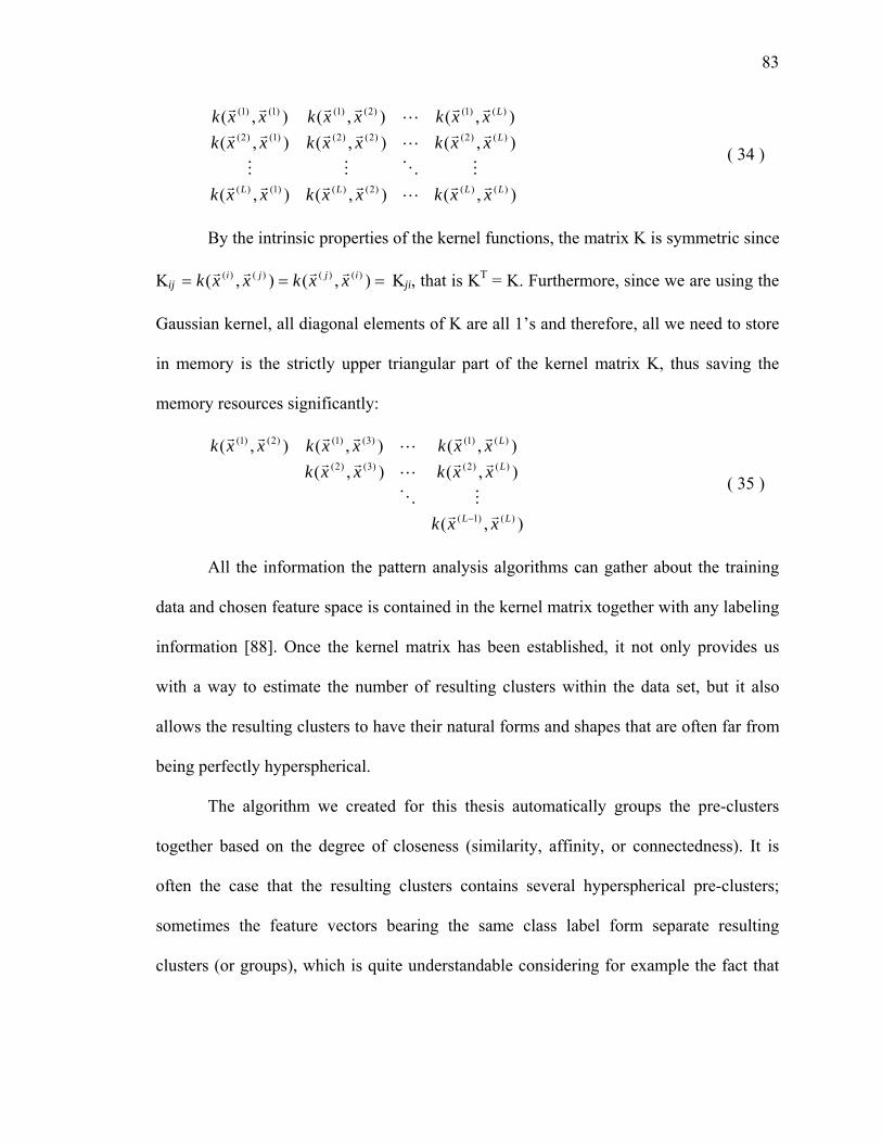
83
),(),(),(
),(),(),(),(),(),(
)()()2()()1()(
)()2()2()2()1()2(
)()1()2()1()1()1(
LLLL
L
L
xxkxxkxxk
xxkxxkxxkxxkxxkxxk
rrL
rrrrMOMM
rrL
rrrr
rrL
rrrr
( 34 )
By the intrinsic properties of the kernel functions, the matrix K is symmetric since
Kij === ),(),( )()()()( ijji xxkxxk rrrr Kji, that is KT = K. Furthermore, since we are using the
Gaussian kernel, all diagonal elements of K are all 1’s and therefore, all we need to store
in memory is the strictly upper triangular part of the kernel matrix K, thus saving the
memory resources significantly:
),(
),(),(),(),(),(
)()1(
)()2()3()2(
)()1()3()1()2()1(
LL
L
L
xxk
xxkxxkxxkxxkxxk
rrMO
rrL
rr
rrL
rrrr
−
( 35 )
All the information the pattern analysis algorithms can gather about the training
data and chosen feature space is contained in the kernel matrix together with any labeling
information [88]. Once the kernel matrix has been established, it not only provides us
with a way to estimate the number of resulting clusters within the data set, but it also
allows the resulting clusters to have their natural forms and shapes that are often far from
being perfectly hyperspherical.
The algorithm we created for this thesis automatically groups the pre-clusters
together based on the degree of closeness (similarity, affinity, or connectedness). It is
often the case that the resulting clusters contains several hyperspherical pre-clusters;
sometimes the feature vectors bearing the same class label form separate resulting
clusters (or groups), which is quite understandable considering for example the fact that

84
some important attribute (or features) that cause the vectors with the same class label be
in some way different are subtle or failed to be captured by the feature extraction
procedure. Sometimes the outliers could be the reason for that. The outliers can be a part
of the data as a result of some type of errors in measurements or malfunctioning of
reading device.
One of the major advantages of the current algorithms is that it enables us to
identify the outliers and mislabeled samples during the training phase and either eliminate
them from the data set completely or significantly decrease their influence on the results
of classification accuracy during the pattern recognition phase.
After the algorithm groups the pre-clusters together in the resulting clusters, it
labels each cluster (going largely to what had been previously described for other
clustering algorithms). The advantage of this algorithm is that since we don’t force the
resulting clusters to be hyperspherical but rather let them have their natural shape, the
confidence in the class label is significantly higher for this particular algorithm than in
the case of clustering by the improved k-means and fuzzy c-means algorithms described
above.
To process unseen before feature vectors with the intent of labeling them, the
algorithm uses the discriminant function:
),()( )( jj vxkxf rrr
= ( 36 )
where )(xf jr is a discriminant function applied to an unlabeled feature vector xr
over cluster j; )( jvr is a center of the j-th cluster (or just a feature vector from the training
data set in case of outliers or small training data sets); ),( )( jvxk rr is a Gaussian kernel, and

85
the parameter σ used in that kernel function is either a variance of cluster j or some
fraction of the average distances between all pairs in the reduced data set. The cluster that
produces the largest value of the discriminant function is considered to be a winner.
Then, the unlabeled feature vector gets the same class label as the winning cluster has.
The confidence in the assigned class labeled is solidly based on the percentage of feature
vectors with the same label over all feature vectors that found to be fuzzy connected
through the kernel matrix and were grouped into the same cluster.
We implemented the fuzzy connectivity clustering (FCC) algorithm in C++ using
the object-oriented approach (see Appendix B for implementation details). The OOP of
FCC algorithm implementation is highly beneficial compared to the procedural approach
that was used in our other implementations: it reduces the program’s complexity
significantly, makes the program interface more informative and considerably increases
the overall program’s clarity, and more importantly, it facilitates the maintainability of
the program and substantially simplifies further modifications, changes, and extensions of
the program.
Next, the FCC algorithm was tested by using the Wisconsin breast cancer data set
as a benchmark data set. While tuning the parameters of the FCC algorithm to reach out
the highest possible classification accuracy, we found that the range of the number of
possible pre-clusters created during the execution of the algorithm is one of the
parameters that the current algorithm is very sensitive to.
It has been shown that the best classification results were obtained when we set
the number of possible pre-clusters between times 2 and times 4 of the number of
available classes in the set. The following table shows the results for different number of
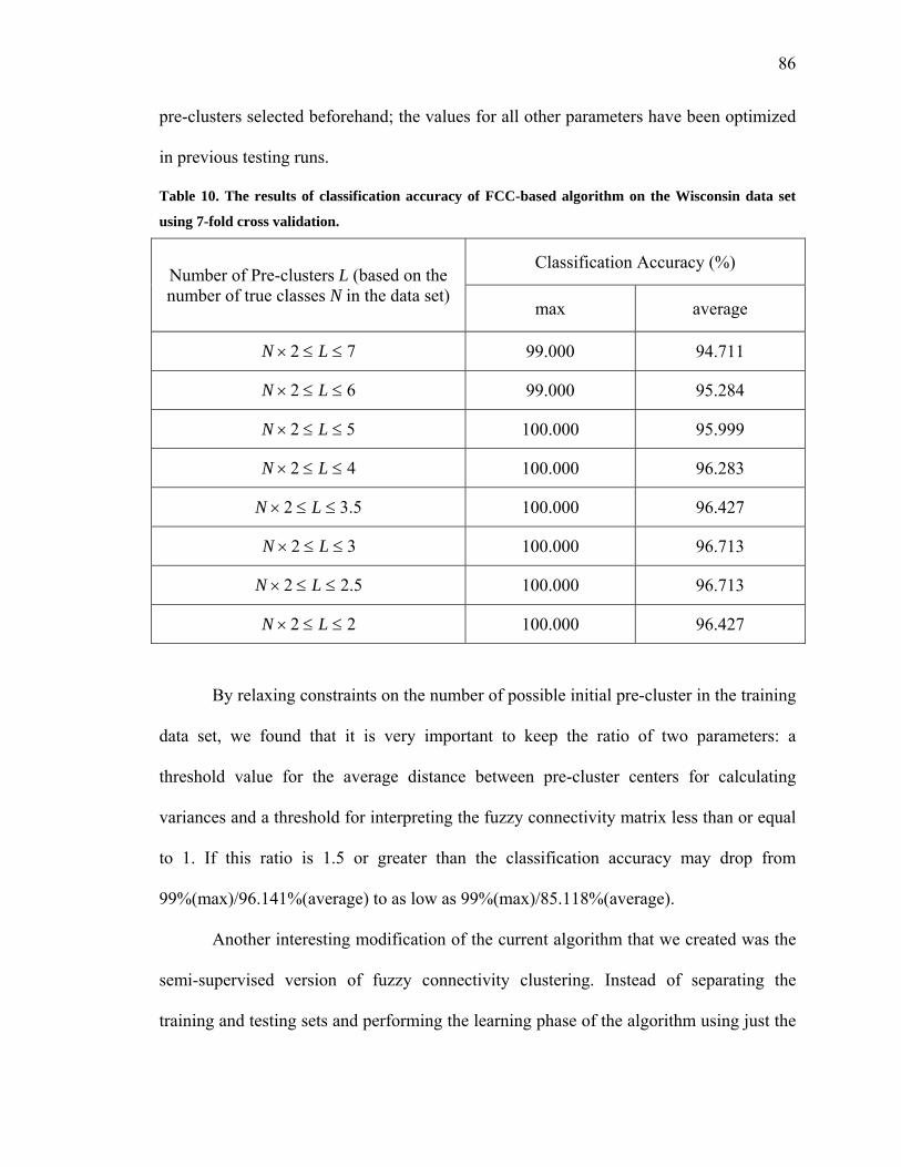
86
pre-clusters selected beforehand; the values for all other parameters have been optimized
in previous testing runs.
Table 10. The results of classification accuracy of FCC-based algorithm on the Wisconsin data set
using 7-fold cross validation.
Number of Pre-clusters L (based on the number of true classes N in the data set)
Classification Accuracy (%)
max average
72 ≤≤× LN 99.000 94.711
62 ≤≤× LN 99.000 95.284
52 ≤≤× LN 100.000 95.999
42 ≤≤× LN 100.000 96.283
5.32 ≤≤× LN 100.000 96.427
32 ≤≤× LN 100.000 96.713
5.22 ≤≤× LN 100.000 96.713
22 ≤≤× LN 100.000 96.427
By relaxing constraints on the number of possible initial pre-cluster in the training
data set, we found that it is very important to keep the ratio of two parameters: a
threshold value for the average distance between pre-cluster centers for calculating
variances and a threshold for interpreting the fuzzy connectivity matrix less than or equal
to 1. If this ratio is 1.5 or greater than the classification accuracy may drop from
99%(max)/96.141%(average) to as low as 99%(max)/85.118%(average).
Another interesting modification of the current algorithm that we created was the
semi-supervised version of fuzzy connectivity clustering. Instead of separating the
training and testing sets and performing the learning phase of the algorithm using just the
87
training set, we combined both sets (leaving feature vectors from the testing set
unlabeled) and performed initial pre-clustering followed by the linking procedure through
the kernel matrix over the entire data set. This idea makes a lot of sense because it
simplifies the algorithm quite significantly while keeping classification accuracy almost
as high as in the original longer version. The results for classification accuracy for this
version varied between 100%(max)/96.284% (average) under the constraints that the
number of pre-clusters should be at most 3.5 times greater than the number of true classes
in the set and 100%(max)/96.426% (average) without such a constraint.
Interestingly, by eliminating a few feature vectors from the data set (less than 4%)
that have been consistently misclassified or linked with feature vectors from the “wrong”
class, we easily reached almost 100% in the classification accuracy on average (for both
modifications of the algorithm).

88
5 Experimental Results
For the current thesis, we collected experimental results using the same
microfabricated cantilever sensor array. This sensor array had been extensively exploited
for the experimental testing for nearly three months, which significantly exceeded the
most optimistic estimate of its life expectancy.
After removing especially noisy and inconsistent data, we obtained 85
34-dimensional feature vectors from nine different classes:
Table 11. Class labels according to the presence of the specified concentration of different chemical
vapors in the analyzed gaseous mixture and the number of feature vectors in each class.
Analyte
26% 18% 7%
Class Number
Number of Vectors
Class Number
Number of Vectors
Class Number
Number of Vectors
Acetone 1 11 2 29 3 6
Ethanol 4 7 5 6 6 7
Toluene 7 11 8 3 9 8
Although we kept the experimental conditions identical throughout all
experiments, the collected data were not of equal quality. The data gathered during the
last month of the testing experiments revealed that the sensor array was quite worn out
from the intensive use. Most of polymer coating materials lost some of their initial
properties after many adsorption-desorption cycles. The best indication of the exhaustion
of some coatings were higher baselines, which are the responses to the “empty” samples,
i.e., the samples of the dry air that do not contain any chemical vapors, and lower

89
responses to the samples contain the target chemical vapors. We found out that some
polymer coatings could not be completely “refreshed” (brought to the initial state) after
the long use. The experimental data of the gaseous mixtures containing toluene vapors
(classes 7 through 9) were collected during the last month of the testing when the quality
of the sensor was somewhat degraded. We believe that this fact largely contributed to the
higher rate of misclassification of the toluene containing data in some cases. Therefore,
we did not consider the data items of class 7 through 9 to be completely reliable to make
any judgment about the algorithm’s performance and used those data very sparsely for
the algorithm’s performance evaluation.
We ran a large number of tests in which feature vectors from the different
combinations of classes were presented, but in this thesis we used only a few most typical
combinations of classes for comparison purposes to illustrate the relative effectiveness
and accuracy of the pattern recognition algorithms. In most cases, the complete n-fold
cross validation technique was used to evaluate the algorithm’s accuracy. We tried to
keep the training/testing data set pairs in each case unique as much as possible. If the
number of feature vectors belonging to the same class in the data set was large enough,
we created testing sets without duplicates between them; otherwise, if the duplicates were
unavoidable, we used different combinations of unlabeled feature vectors in each testing
set. All testing sets were created in such a way that the number of feature vectors in the
testing data set from a specific class is directly proportional to the number of feature
vectors with the same label in the combined data set (both training and testing data sets
combined together) and all class labels are present in the testing data set. The order of the
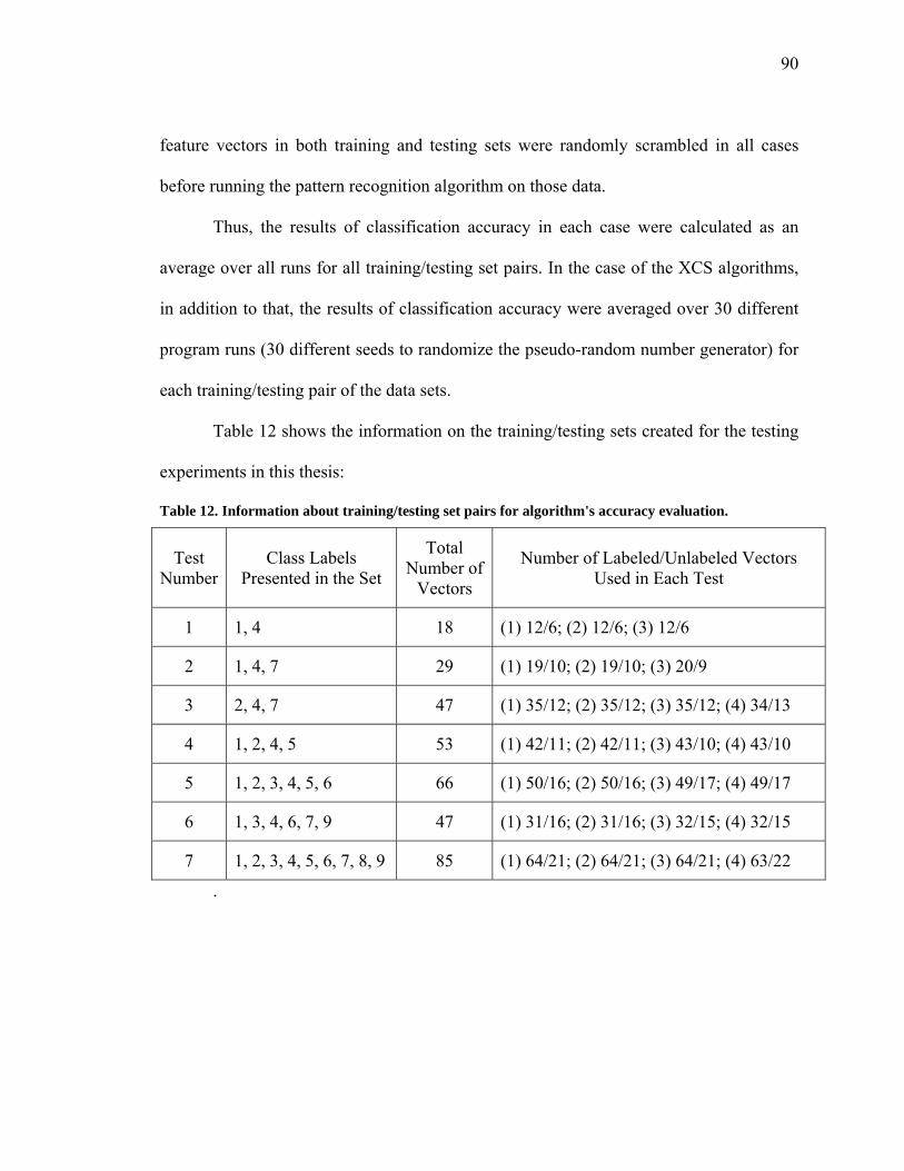
90
feature vectors in both training and testing sets were randomly scrambled in all cases
before running the pattern recognition algorithm on those data.
Thus, the results of classification accuracy in each case were calculated as an
average over all runs for all training/testing set pairs. In the case of the XCS algorithms,
in addition to that, the results of classification accuracy were averaged over 30 different
program runs (30 different seeds to randomize the pseudo-random number generator) for
each training/testing pair of the data sets.
Table 12 shows the information on the training/testing sets created for the testing
experiments in this thesis:
Table 12. Information about training/testing set pairs for algorithm's accuracy evaluation.
Test Number
Class Labels Presented in the Set
Total Number of
Vectors
Number of Labeled/Unlabeled Vectors Used in Each Test
1 1, 4 18 (1) 12/6; (2) 12/6; (3) 12/6
2 1, 4, 7 29 (1) 19/10; (2) 19/10; (3) 20/9
3 2, 4, 7 47 (1) 35/12; (2) 35/12; (3) 35/12; (4) 34/13
4 1, 2, 4, 5 53 (1) 42/11; (2) 42/11; (3) 43/10; (4) 43/10
5 1, 2, 3, 4, 5, 6 66 (1) 50/16; (2) 50/16; (3) 49/17; (4) 49/17
6 1, 3, 4, 6, 7, 9 47 (1) 31/16; (2) 31/16; (3) 32/15; (4) 32/15
7 1, 2, 3, 4, 5, 6, 7, 8, 9 85 (1) 64/21; (2) 64/21; (3) 64/21; (4) 63/22
.

91
5.1 Extended Classifier System (XCS)
The poor performance of the XCS algorithm using our experimental sensory data
came as no surprise (see Table 13). We can observe how classification accuracy has been
constantly dropping as the number of possible classes in the data set increases.
Table 13. The results of classification accuracy of the XCS algorithm using the cantilever sensor
array data.
Test Number
Class Labels Presented in the Set
Classification Accuracy (%)
average of max average of average
1 1, 4 75.555 64.815
2 1, 4, 7 46.556 36.099
3 2, 4, 7 53.184 41.309
4 1, 2, 4, 5 43.485 29.765
5 1, 2, 3, 4, 5, 6 28.217 22.702
6 1, 3, 4, 6, 7, 9 31.488 21.964
7 1, 2, 3, 4, 5, 6, 7, 8, 9 14.286 9.470
There are two main reasons for such low classification accuracy of XCS in the
case of our sensory data.
The first reason for that is a small number of feature vectors in the training set.
This algorithm was originally designed to learn on a sufficiently large number of the
input vectors. As we found out testing this algorithm on the benchmark data sets, in order
to reach the peak of its ability to classify a new input vector highly accurate, the
population of classifiers of XCS should contain a large number of very experienced

92
classifiers, where the number of input vectors Q should be much greater than the number
of features N in each vector, Q >> N. This condition is obviously not possible without a
sufficiently large training data set.
The second reason for low classification of XCS is the way we used to encode the
feature values into the binary numbers, that is we used only one bit to encode each
number n: if n < 0.5, then use 0; otherwise, use 1 to encode that number. There is hope
that by increasing of a number of bits that are used to encode each feature value into a
binary number, we can increase the accuracy of each classifier in the system, hence
increase the classification accuracy of the XCS algorithm as a whole.
5.2 Radial Basis Function Neural Network (RBF NN)
Just slightly better were the results of classification accuracy of the RBF NN
algorithm on the cantilever sensor array experimental data (see Table 14). The reasons for
its poor performance are similar to those of the XCS algorithm: a small number of
training set compare to the high vector dimensionality and a relatively large number of
different classes in the data set compared to the total number of the feature vectors.
These results are in complete agreement with our initial assumption that the
conventional neural network algorithms are not quite suitable for use with the cantilever
sensor array data, when the pattern recognition algorithm should be able to extract all
needed information about the data from a considerably small number of the exemplar
vectors.

93
Table 14. The results of classification accuracy of the RBF NN algorithm using the cantilever sensor
array data.
Test Number
Class Labels Presented in the Set
Classification Accuracy (%)
max average
1 1, 4 50.000 50.000
2 1, 4, 7 55.560 41.853
3 2, 4, 7 58.330 55.285
4 1, 2, 4, 5 50.000 35.908
5 1, 2, 3, 4, 5, 6 37.500 33.363
6 1, 3, 4, 6, 7, 9 26.670 24.168
7 1, 2, 3, 4, 5, 6, 7, 8, 9 28.570 27.055
5.3 Support Vector Machines (SVMs)
Traditionally, the SVM algorithm is considered to be the best performer among
other pattern recognition algorithms for the data sets that contain a small number of the
highly dimensional feature vectors.
However, as we can see from the testing results provided below (Table 15, Table
16, and Table 17), the SVM algorithm performs well only on the data from the limited
number of classes. Once the diversity of the feature vectors in the same data set increases,
classification accuracy of the SVM algorithm drops (sometimes significantly). Even
though the Gaussian kernel is typically considered to be the best choice for the kernel, in
our case the best classification accuracy was obtained with the use of the simplest kernel
function, the linear kernel.
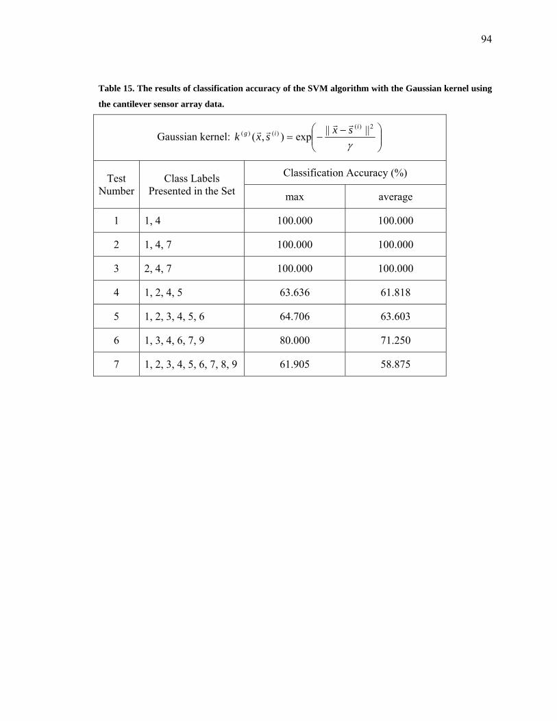
94
Table 15. The results of classification accuracy of the SVM algorithm with the Gaussian kernel using
the cantilever sensor array data.
Gaussian kernel: ⎟⎟⎠
⎞⎜⎜⎝
⎛ −−=
γ
2)()()( ||||exp),(
iig sxsxk
rrrr
Test Number
Class Labels Presented in the Set
Classification Accuracy (%)
max average
1 1, 4 100.000 100.000
2 1, 4, 7 100.000 100.000
3 2, 4, 7 100.000 100.000
4 1, 2, 4, 5 63.636 61.818
5 1, 2, 3, 4, 5, 6 64.706 63.603
6 1, 3, 4, 6, 7, 9 80.000 71.250
7 1, 2, 3, 4, 5, 6, 7, 8, 9 61.905 58.875

95
Table 16. The results of classification accuracy of the SVM algorithm with the linear kernel using the
cantilever sensor array data.
Linear kernel: )()()( ),( iil sxsxk rrrr⋅=
Test Number
Class Labels Presented in the Set
Classification Accuracy (%)
max average
1 1, 4 100.000 100.000
2 1, 4, 7 100.000 100.000
3 2, 4, 7 100.000 100.000
4 1, 2, 4, 5 81.818 78.409
5 1, 2, 3, 4, 5, 6 88.235 86.397
6 1, 3, 4, 6, 7, 9 100 98.333
7 1, 2, 3, 4, 5, 6, 7, 8, 9 85.714 82.413
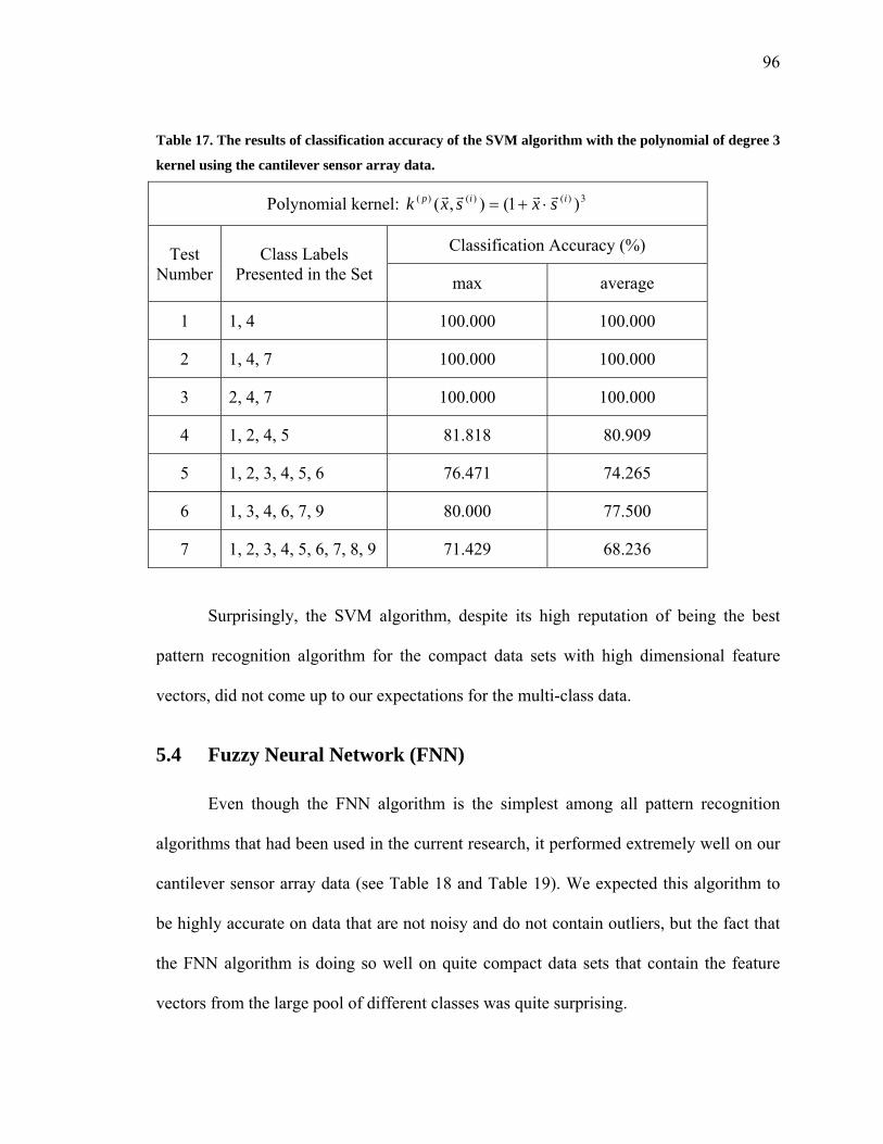
96
Table 17. The results of classification accuracy of the SVM algorithm with the polynomial of degree 3
kernel using the cantilever sensor array data.
Polynomial kernel: 3)()()( )1(),( iip sxsxk rrrr⋅+=
Test Number
Class Labels Presented in the Set
Classification Accuracy (%)
max average
1 1, 4 100.000 100.000
2 1, 4, 7 100.000 100.000
3 2, 4, 7 100.000 100.000
4 1, 2, 4, 5 81.818 80.909
5 1, 2, 3, 4, 5, 6 76.471 74.265
6 1, 3, 4, 6, 7, 9 80.000 77.500
7 1, 2, 3, 4, 5, 6, 7, 8, 9 71.429 68.236
Surprisingly, the SVM algorithm, despite its high reputation of being the best
pattern recognition algorithm for the compact data sets with high dimensional feature
vectors, did not come up to our expectations for the multi-class data.
5.4 Fuzzy Neural Network (FNN)
Even though the FNN algorithm is the simplest among all pattern recognition
algorithms that had been used in the current research, it performed extremely well on our
cantilever sensor array data (see Table 18 and Table 19). We expected this algorithm to
be highly accurate on data that are not noisy and do not contain outliers, but the fact that
the FNN algorithm is doing so well on quite compact data sets that contain the feature
vectors from the large pool of different classes was quite surprising.

97
Table 18. The results of classification accuracy of the FNN algorithm with the discriminant function
f 1 using the cantilever sensor array data.
},...,1:),({max{)( )(1jj
qj Qqxxkxf j ==
rrr
Test Number
Class Labels Presented in the Set
Classification Accuracy (%)
max average
1 1, 4 100.000 100.000
2 1, 4, 7 100.000 100.000
3 2, 4, 7 100.000 100.000
4 1, 2, 4, 5 100.000 92.728
5 1, 2, 3, 4, 5, 6 100.000 92.463
6 1, 3, 4, 6, 7, 9 100.000 96.770
7 1, 2, 3, 4, 5, 6, 7, 8, 9 95.240 87.230
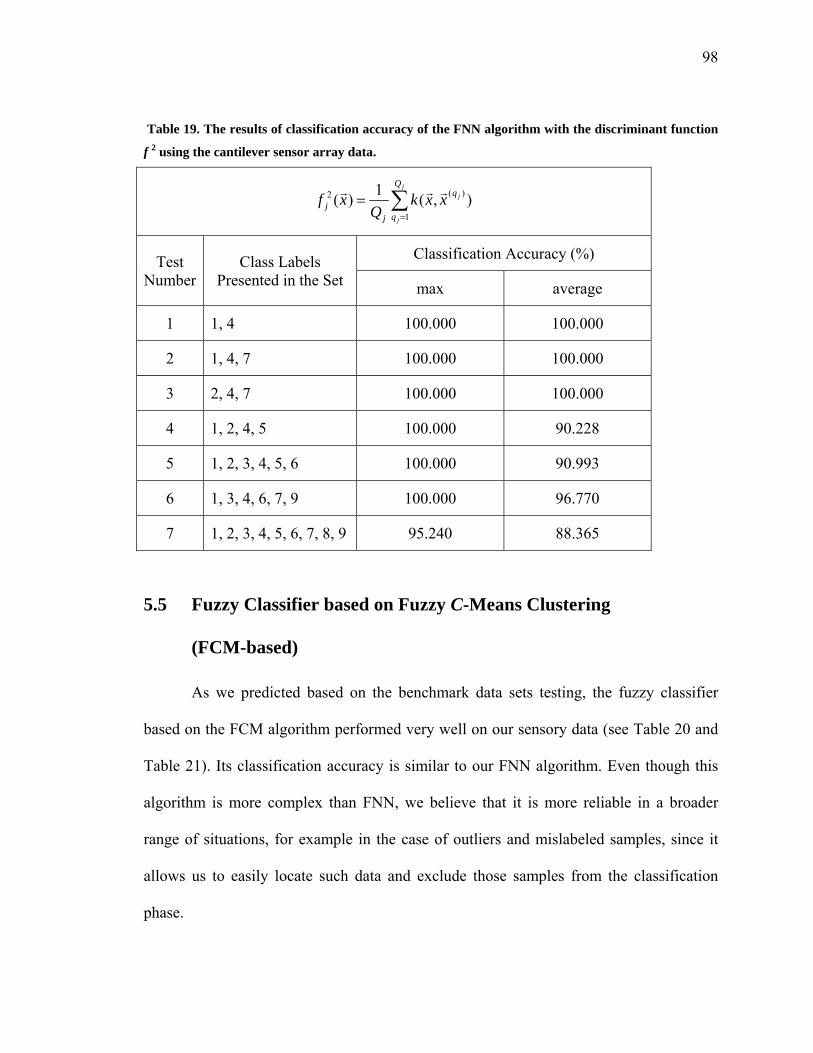
98
Table 19. The results of classification accuracy of the FNN algorithm with the discriminant function
f 2 using the cantilever sensor array data.
∑=
=j
j
j
Q
q
q
jj xxk
Qxf
1
)(2 ),(1)( rrr
Test Number
Class Labels Presented in the Set
Classification Accuracy (%)
max average
1 1, 4 100.000 100.000
2 1, 4, 7 100.000 100.000
3 2, 4, 7 100.000 100.000
4 1, 2, 4, 5 100.000 90.228
5 1, 2, 3, 4, 5, 6 100.000 90.993
6 1, 3, 4, 6, 7, 9 100.000 96.770
7 1, 2, 3, 4, 5, 6, 7, 8, 9 95.240 88.365
5.5 Fuzzy Classifier based on Fuzzy C-Means Clustering
(FCM-based)
As we predicted based on the benchmark data sets testing, the fuzzy classifier
based on the FCM algorithm performed very well on our sensory data (see Table 20 and
Table 21). Its classification accuracy is similar to our FNN algorithm. Even though this
algorithm is more complex than FNN, we believe that it is more reliable in a broader
range of situations, for example in the case of outliers and mislabeled samples, since it
allows us to easily locate such data and exclude those samples from the classification
phase.

99
Table 20. The results of classification accuracy of the fuzzy classifier based on FCM-based algorithm
with the discriminant function f 1 using the cantilever sensor array data.
),()( )(1 jj vxkxf rrr
=
Test Number
Class Labels Presented in the Set
Classification Accuracy (%)
max average
1 1, 4 100.000 100.000
2 1, 4, 7 100.000 100.000
3 2, 4, 7 100.000 100.000
4 1, 2, 4, 5 100.000 87.728
5 1, 2, 3, 4, 5, 6 100.000 88.143
6 1, 3, 4, 6, 7, 9 100.000 96.668
7 1, 2, 3, 4, 5, 6, 7, 8, 9 90.480 85.875
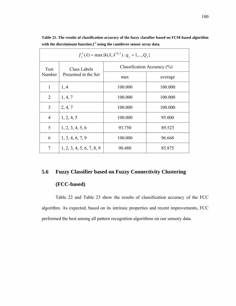
100
Table 21. The results of classification accuracy of the fuzzy classifier based on FCM-based algorithm
with the discriminant function f 2 using the cantilever sensor array data.
},...,1:),(max{)( )(2jj
qj Qqxxkxf j ==
rrr
Test Number
Class Labels Presented in the Set
Classification Accuracy (%)
max average
1 1, 4 100.000 100.000
2 1, 4, 7 100.000 100.000
3 2, 4, 7 100.000 100.000
4 1, 2, 4, 5 100.000 95.000
5 1, 2, 3, 4, 5, 6 93.750 89.523
6 1, 3, 4, 6, 7, 9 100.000 96.668
7 1, 2, 3, 4, 5, 6, 7, 8, 9 90.480 85.875
5.6 Fuzzy Classifier based on Fuzzy Connectivity Clustering
(FCC-based)
Table 22 and Table 23 show the results of classification accuracy of the FCC
algorithm. As expected, based on its intrinsic properties and recent improvements, FCC
performed the best among all pattern recognition algorithms on our sensory data.

101
Table 22. The results of classification accuracy of the semi-supervised version of the FCC-based
algorithm using the cantilever sensor array data.
Semi-supervised Clustering (Short Version):
labeled and unlabeled feature vectors are clustered together
Test Number
Class Labels Presented in the Set
Classification Accuracy (%)
max average
1 1, 4 100.000 96.667
2 1, 4, 7 100.000 97.917
3 2, 4, 7 100.000 100.000
4 1, 2, 4, 5 100.000 100.000
5 1, 2, 3, 4, 5, 6 100.000 92.463
6 1, 3, 4, 6, 7, 9 100.000 93.542
7 1, 2, 3, 4, 5, 6, 7, 8, 9 95.238 87.175

102
Table 23. The results of classification accuracy of the full version of the FCC-based algorithm that
clustered labeled vectors separately from unlabeled ones using the cantilever sensor array data.
Unsupervised Clustering (Full Version):
labeled feature vectors are clustered separately from unlabeled
Test Number
Class Labels Presented in the Set
Classification Accuracy (%)
max average
1 1, 4 100.000 100.000
2 1, 4, 7 100.000 100.000
3 2, 4, 7 100.000 100.000
4 1, 2, 4, 5 100.000 100.000
5 1, 2, 3, 4, 5, 6 100.000 97.059
6 1, 3, 4, 6, 7, 9 100.000 95.000
7 1, 2, 3, 4, 5, 6, 7, 8, 9 100.000 90.639

103
6 Conclusion and Future Work
Within the framework of the current research several objectives have been
achieved.
It has been found that the information extracted from just the resonance frequency
shifts of cantilever sensors in the microfabricated array during exposure of the array to
the target analyte vapors is mostly sufficient for creating fingerprints of the analytes. The
measured resonance frequency shift responses of the cantilevers can be used as an input
to the variety of pattern recognition algorithms for the purpose of creating a reliable
system that is capable of detecting and recognizing a variety of target analytes and
quantitative estimation of the relative concentration of those analyte vapors in a gaseous
mixture, for example in the ambient air.
During the multiple experiments with microfabricated cantilever sensors it has
been demonstrated that the use of the array of cantilevers with some of cantilevers being
functionalized by coating their surface with thoroughly chosen commercial polymers has
significantly improved the selectivity of the sensor array as a whole to the target analytes.
As a result of experimental work, the cantilever resonance frequency responses
during exposure of the array of cantilever sensors to the dry air and the air containing
different concentration (high – 26%, medium – 18%, and low – 7%) of vapors of the three
different organic solvents: acetone, ethanol, and toluene, have been collected.
After careful examination, the procedure of extracting the most important
information out of 7000 different measurements for each sample has been created. By
104
applying the created strategy for feature extraction, the data set of 34-dimensional feature
vectors has been created.
The main goal of the current research was to create pattern recognition algorithms
that can be effectively used as a reliable detection system with the specific sensory data
obtained during the experiments with a microfabricated cantilever sensor array and
further feature extracting procedure.
Five different pattern recognition algorithms have been created for the current
research. All of those algorithms and the open source implementation of the sixth
algorithm (multiclass SVMs) were used for testing on benchmark data sets and collected
sensory data. It has been shown that the kernel-based algorithms have the greatest
potential to be used with the microfabricated cantilever sensor array in the detection
systems. Four out of six pattern recognition algorithms have produced high accuracy
classification results upon processing the cantilever sensor array data.
Despite the fact that the extended classifier system (XCS) algorithm showed quite
a good performance on the benchmark data sets, it failed to produce equally good
classification results on our sensory data. Even though we believe that XCS could be
successfully modified to accommodate specific properties of the sensory data, especially
a very small size of the data set and high dimensionality of the feature vectors, in order to
increase its classification accuracy, we do not consider this algorithm as a good choice
for the cantilever sensor array detection system.
It has been also shown that the radial basis function neural network (RBF NN)
algorithm is not especially effective in the case of small training data sets, high
105
dimensionality of the feature vectors, and multiclass environment. We believe that further
attempts to employ the neural networks as a pattern recognition algorithm to be used with
a microcantilever sensor array for detection, recognition, and quantitative estimation of
the target analytes do not hold considerable promise.
The SVM algorithm has a solid reputation of being the best performer in the case
of the limited number of high dimensional feature vectors available for training.
However, this algorithm is very sensitive to the noisy data and outliers. Since the sensory
data are prone to suffer from noise and a variety of reading device errors, the SVM
algorithm cannot be one hundred percent reliable in every situation that may be
encountered during the detection process. Besides, it has been demonstrated that the
classification accuracy of the SVM algorithm dropped significantly with the increase of
the number of different classes in the limited experimental data. However, in many cases,
SVM still might provide satisfying results and therefore, can be cautiously used as a part
of the detection system.
Fuzzy logic and the notion of fuzziness provide a useful framework for
representing uncertainty in the sensory data. It has been shown that the fuzzy approach to
creating a reliable classifier system is particularly relevant for the cantilever sensor array
data. The fuzzy neural network (FNN) algorithm that is essentially the kernel-based fuzzy
classifier has produced the excellent results on the cantilever sensor array data. This
algorithm is very simple and asymptotically very efficient. In the case of absence of the
outliers and mislabeled samples, it should be the first choice for the pattern recognition
algorithm to be used with sensory data.

106
However, the noisy data and outliers are quite common among the cantilever
sensor array data. In this thesis it has been shown that a combination of a clustering
analysis, as a pre-processing technique, and a fuzzy classifier creates a powerful tool for
the simultaneous, accurate, fast, more reliable and robust detection and identification of
the target analytes in a gaseous mixture with the use of a microcantilever sensor array.
The combination of unsupervised and semi-supervised data analysis of the labeled
training data set allows identifying the outliers and mislabeled data and creating a basis
for the highly precise fuzzy classifiers to be used for unseen before data samples. It has
been determined that fuzzy classifiers based on the fuzzy c-means clustering and fuzzy
connectivity clustering algorithms clearly outperformed the traditionally used neural
networks and in some cases even the SVM algorithm and could be considered as the most
promising pattern recognition algorithms to be used with the microcantilever sensor array
as a selective and quantitative chemical detection system.
Thus, in this thesis it has been demonstrated that a micromechanical array of
cantilever sensors can be used in combination with the certain types of pattern
recognition algorithms to examine the gaseous mixtures and detect target analytes with
high accuracy (100% in most cases). A combination of a clustering analysis and fuzzy
classifiers creates a family of powerful pattern recognition algorithms for the cantilever
sensor array data. In the case of consistent and noiseless sensory data FNN could be the
best choice for the pattern recognition algorithm.
Future work needs to be focused on the further modification of the mentioned
above kernel-based fuzzy classifier algorithms as a part of the detection systems. There

107
are some useful features that can be easily incorporated into those algorithms. For
example, 1) the automatic detection of the noisy data and outliers and removing them
from the training data sets, and 2) calculating the standard deviation of a cluster based on
the density of the feature vectors in it, instead of the averaged distances between feature
vectors and a center of the cluster.
Another research area that should be given close attention is an analysis of the
analyte mixtures. The preliminary test results with binary mixtures of acetone and ethanol
vapors obtained during the current research are highly supportive of the idea that these
pattern recognition algorithms are precisely the right method for the detection,
identification, and quantitative estimation of every component in the complex mixtures of
the target analytes, even in the absence of exhaustive training data. Therefore, more
studies have to be done in that direction as well. This ability to successfully analyze
analytes’ mixtures will greatly increase the range of classification of the detection system
and help to meet increasing demand for such systems.

108
7 Appendices
7.1 Appendix A – Implementation Details of XCS Algorithm
The XCS classifier system has been fully implemented in C++ using the object-
oriented approach. For this purpose, five classes have been created:
1. Class Counter – responsible for creating a unique identification number for each
classifier as well as for keeping track of the total number of the GA performed.
2. Class Clock – responsible for time stamping each classifier at birth and updating
the time-stamp every time the classifier happens to be in [A] during the GA. This
class also keeps track of the time when explore approach in selecting the action in
[A] has been used.
3. Class Input – responsible for creating input strings to send to the classifier
systems and all operation related to the input.
4. Class Classifier – responsible for creating classifiers, as well as for all operation
related to the classifiers.
5. Class XCS – responsible for creating the entire classifier system that contains
members of both Input and Classifier classes (along with the others) and running
the algorithm throughout the entire experiment.
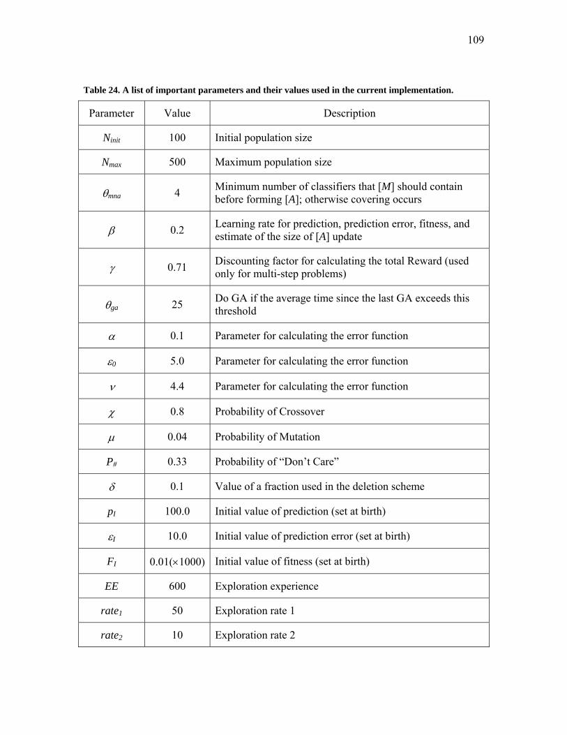
109
Table 24. A list of important parameters and their values used in the current implementation.
Parameter Value Description
Ninit 100 Initial population size
Nmax 500 Maximum population size
θmna 4 Minimum number of classifiers that [M] should contain before forming [A]; otherwise covering occurs
β 0.2 Learning rate for prediction, prediction error, fitness, and estimate of the size of [A] update
γ 0.71 Discounting factor for calculating the total Reward (used only for multi-step problems)
θga 25 Do GA if the average time since the last GA exceeds this threshold
α 0.1 Parameter for calculating the error function
ε0 5.0 Parameter for calculating the error function
ν 4.4 Parameter for calculating the error function
χ 0.8 Probability of Crossover
μ 0.04 Probability of Mutation
P# 0.33 Probability of “Don’t Care”
δ 0.1 Value of a fraction used in the deletion scheme
pI 100.0 Initial value of prediction (set at birth)
εI 10.0 Initial value of prediction error (set at birth)
FI 0.01(×1000) Initial value of fitness (set at birth)
EE 600 Exploration experience
rate1 50 Exploration rate 1
rate2 10 Exploration rate 2
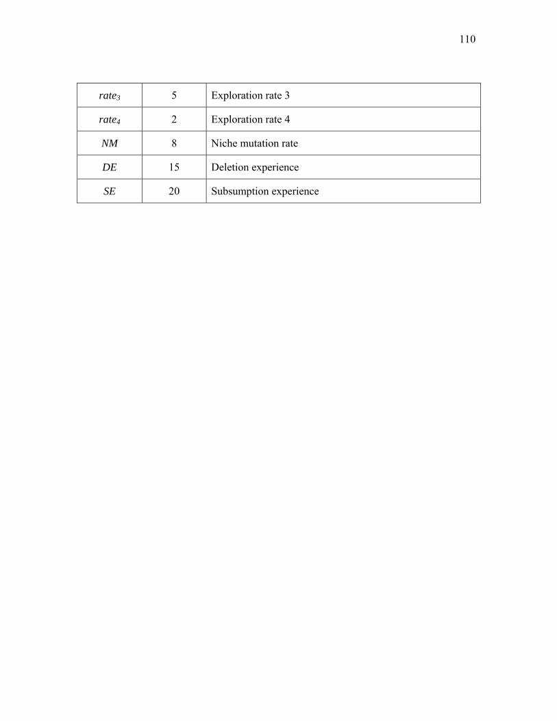
110
rate3 5 Exploration rate 3
rate4 2 Exploration rate 4
NM 8 Niche mutation rate
DE 15 Deletion experience
SE 20 Subsumption experience

111
7.2 Appendix B – Implementation Details of FCC Algorithm
WrappedUpFCM
Vector
SystemInfo
Interpreter
LabelFCM
System
Group
PartSet
Set FeatureVector
StatSet
Result
OutFCM
Figure 22. Class diagram of the OOP implementation of the FCC algorithms.

112
8 References
[1] S. Zaromb and J.R. Stetter, “Theoretical basis for identification and measurement
of air contaminants using an array of sensors having partly overlapping
selectivities,” Sensors and Actuators, vol. 6(4), pp. 225−243, 1984.
[2] H. Abe, T. Yoshimura, S. Kanaya, Y. Takahashi, Y. Miyashita, and S.-I. Sasaki,
“Automated odor-sensing system based on plural semiconductor gas sensors and
computerized pattern recognition techniques,” Analytica Chimica Acta, vol. 194,
pp. 1−9, 1987.
[3] H. Abe, S. Kanaya, Y. Takahashi, and S.-I. Sasaki, “Extended studies of the
automated odor-sensing system based on plural semiconductor gas sensors with
computerized pattern recognition techniques,” Analytica Chimica Acta, vol. 215,
pp. 155−168, 1988.
[4] T. Thundat, P.I. Oden, and R.J. Warmack, “Microcantilever Sensors,” Microscale
Thermophysical Engineering, vol. 1(3), pp. 185−199, 1997.
[5] N. Abedinov, C. Popov, Zh. Yordanov, Tzv. Ivanov, T. Gotszalk, P. Grabiec, W.
Kulisch, I.W. Rangelow, D. Filenko, and Yu. Shirshov, “Chemical recognition
based on micromachined silicon cantilever array,” J. Vacuum Science &
Technology: B, vol. 21(6), pp. 2931−2936, 2003.
[6] N.V. Lavrik, M.J. Sepaniak, P.G. Datskos, “Cantilever transducers as a platform
for chemical and biological sensors,” Review of Scientific Instruments, vol. 75(7),
pp. 2229−2953, 2004.

113
[7] H.P. Lang, M. Hegner and Ch. Gerber, “Microfabricated Cantilever Array Sensors
for (Bio-)Chemical Detection,” In: B. Bhushan and H. Fuchs (Eds.), “Applied
Scanning Probe Methods IV – Industrial Applications,” Springer-Verlag, Berlin,
New York, Heidelberg, Chapter 28, pp. 183−213, 2006.
[8] J.W. Grate and D.A. Nelson, “Sorptive polymeric materials and photopatterned
films for gas phase chemical microsensors,” Proc. IEEE, vol. 91(6), pp. 881−889,
2003.
[9] R. Gutierrez-Osuna, “Pattern analysis for machine olfaction: a review,” IEEE
Sensors Journal, vol. 2(3), pp. 189–202, 2002.
[10] G. Binning, C. F. Quate, and Ch. Gerber, “Atomic Force Microscope,” Physical
Review Letters, vol. 56(9), pp. 930–933, 1986.
[11] H.P. Lang, M. Hegner, Ch. Gerber, "Cantilever Array Sensors,” Materials Today,
vol. 8(4), pp. 30–36, 2005.
[12] R. Berger, E. Delamarche, H.P. Lang, C. Gerber, J.K. Gimzewski, E. Meyer, and
H.-J. Güntherodt, “Surface Stress in the Self-Assembly of Alkanethiols on Gold,”
vol. 276(5321), Science, pp. 2021–2024, 1997.
[13] J. Fritz, M.K. Baller, H.P. Lang, H. Rothuizen, P. Vettiger, E. Meyer, H.-J.
Güntherodt, Ch. Gerber, and J.K. Gimzewski, “Translating Biomolecular
Recognition into Nanomechanics,” Science, vol. 288(5464), pp. 316–318, 2000.
[14] J.P. Cleveland, S. Manne, D. Bocek, P.K. Hansma, “A nondestructive method for
determining the spring constant of cantilevers for scanning force microscopy,”
Review of Scientific Instruments, vol. 64(2), pp. 403–405, 1993.

114
[15] T. Thundat, R.J. Warmack, ”Thermal and ambient-induced deflections of scanning
force microscope cantilevers,” Applied Physics Letters, vol. 64(21), pp. 2894–2896,
1994.
[16] E.A. Wachter, T. Thundat, “Micromechanical sensors for chemical and physical
measurements,” Review of Scientific Instruments, vol. 66(6), pp. 3662–3667, 1995.
[17] J.W. Grate, “Acoustic Wave Microsensor Arrays for Vapor Sensing,” Chemical
Reviews, vol. 100(7), pp. 2627–2648, 2000.
[18] E.T. Zellers, S.A. Batterman, M. Han, S.J. Patrash, , “Optimal coating selection for
the analysis of organic vapor mixtures with polymer-coated surface acoustic wave
sensor arrays,” Analytical Chemistry, vol. 67 (6), pp. 1092–1106, 1995.
[19] M.P. Eastman, R.C. Hughes, G. Yelton, A.J. Ricco, S.V. Patel, and M.W. Jenkins,
“Application of the Solubility Parameter Concept to the Design of Chemiresistor
Arrays,” Journal of the Electrochemical Society, vol. 146(10), pp. 3907–3913,
1999.
[20] F. Bender, L. Wachter, A. Voigt, and M. Rapp, “Deposition of high quality
coatings on SAW sensors using electrospray,” Proc. Second Int. IEEE Conf.
Sensors, vol. 1, pp. 115–119, 2003.
[21] S. Sarkar, N. Levit, and G. Tepper, “Deposition of polymer coatings onto SAW
resonators using AC electrospray,” Sensors and Actuators B, vol. 114(2), pp. 756–
761, 2006.

115
[22] A. Bietsch, J. Zhang, M. Hegner, H.P. Lang, and C. Gerber, “Rapid
functionalization of cantilever array sensors by inkjet printing,” Nanotechnology,
vol. 15(8), pp. 873–880, 2004.
[23] S. Alexander, L. Hellemans, O.Marti, J. Schneir, V. Elings, P.K. Hansma,M.
Longmire, and J. Gurley, “An atomic-resolution atomic-force microscope
implemented using an optical lever,” Journal of Applied Physics, vol. 65(1), pp.
164–167, 1989.
[24] E.A. Wachter, T. Thundat, P.I. Oden, R.J. Warmack, P.G. Datskos, and S.L. Sharp,
“Remote optical detection using microcantilevers,” Review of Scientific
Instruments, vol. 67(10), pp. 3434–3439, 1996.
[25] M. Tortonese, R.C. Barrett, and C.F. Quate, “Atomic resolution with an atomic
force microscope using piezoresistive detection,” Applied Physics Letters,
vol. 62(8), pp. 834–836, 1993.
[26] T.L. Porter, M.P. Eastman, D.L. Pace, and M. Bradley, “Sensor based on
piezoresistive microcantilever technology,” Sensors and Actuators A, vol. 88(1),
pp. 47–51, 2001.
[27] S.A. Miller, K.L. Turner, N.C. MacDonald, “Microelectromechanical scanning
probe instruments for array architectures,” Review of Scientific Instruments,
vol. 68(11), pp. 4155–4162, 1997.
[28] K. K. Park, H. J. Lee, G. G. Yaralioglu, A. S. Ergun, Ö. Oralkan, M. Kupnik, C. F.
Quate, and B. T. Khuri-Yakub, T. Braun, J.-P. Ramseyer, H. P. Lang, M. Hegner,
Ch. Gerber, and J. K. Gimzewski, “Capacitive micromachined ultrasonic
116
transducers for chemical detection in nitrogen,” Applied Physics Letters, vol. 91(9),
pp. 094102-1–094102-3, 2007.
[29] D.L. DeVoe, and A.P. Pisano, “Modeling and optimal design of piezoelectric
cantilever microactuators,” Journal of Microelectromechanical Systems, vol. 6(3),
pp. 266–270, 1997.
[30] T. Itoh, C. Lee, T. Suga, “Deflection detection and feedback actuation using a self-
excited piezoelectric Pb(Zr,Ti)O3 microcantilever for dynamic scanning force
microscopy,” Applied Physics Letters, vol. 69(14), pp. 2036–2038, 1997.
[31] S. Zurn, M. Hsieh, G. Smith, D. Markus, M. Zang, G. Hughes, Y. Nam, M. Arik,
and D. Polla “Fabrication and structural characterization of a resonant frequency
PZT microcantilever,” Smart Materials and Structures, vol. 10(2), pp. 252–263,
2001.
[32] J. D. Adams, G. Parrott, C. Bauer, T. Sant, L. Manning, M. Jones, B. Rogers, D.
McCorkle, and T. L. Ferrell, “Nanowatt chemical vapor detection with a self-
sensing, piezoelectric microcantilever array,” Applied Physics Letters, vol. 83(16),
pp. 3428–3430, 2003.
[33] J. Park, W.A. Groves, and E.T. Zellers, “Vapor Recognition with Small Arrays of
Polymer-Coated Microsensors. A Comprehensive Analysis,” Analytical Chemistry,
vol. 71(17), pp. 3877–3886, 1999.
[34] M.K. Baller, H.P. Lang, J. Fritz, Ch. Gerber, J.K. Gimzewski, U. Drechsler, H.
Rothuizen, M. Despont, P. Vettiger, F.M. Battiston, J.P. Ramseyer, P. Fornaro, E.

117
Meyer, H.-J. Güntherodt, “A cantilever array-based artificial nose,”
Ultramicroscopy, vol. 82(1), pp. 1–9, 2001.
[35] H.P. Lang, J.P. Ramseyer, W. Grange, T. Braun, D. Schmid, P. Hunziker, C. Jung,
M. Hegner, and C. Gerber, “An Artificial Nose Based on Microcantilever Array
Sensors,” Journal of Physics: Conference Series, vol. 61, pp. 663–667, 2007.
[36] M. Penza and G. Cassano, “Application of principal component analysis and
artificial neural networks to recognize the individual VOCs of methanol/2-propanol
in a binary mixture by SAW multi-sensor array,” Sensors and Actuators B,
vol. 89(3), pp. 269–284, 2003.
[37] W.P. Carey, K.R. Beebe, B.R. Kowalski, D.L. Illman, and T. Hirschfeld “Selection
of adsorbates for chemical sensor arrays by pattern recognition,” Analytical
Chemistry, vol. 58(1), pp. 149–153, 1986.
[38] L.R. Senesac, P. Dutta, P.G. Datskos, and M.J. Sepaniak, “Analyte species and
concentration identification using differentially functionalized microcantilever
arrays and artificial neural networks,” Analytica Chimica Acta, vol. 558, pp. 94–
101, 2006.
[39] S.-M. Chang, Y. Iwasaki, M. Suzuki, E. Tamiya, I. Karube, and H. Muramatsu
“Detection of odorants using an array of piezoelectric crystals and neural-network
pattern recognition,” Analytica Chimica Acta, vol. 249(2), pp. 323–329, 2001.
[40] C.D. Natale, F.A.M. Davide, A. D'Amico, A. Hierlemann, J. Mitrovics, M.
Schweizer, U. Weimar, and W. Göpel, “A composed neural network for the
118
recognition of gas mixtures,” Sensors and Actuators B, vol. 24-25, pp. 808–812,
1995.
[41] B.H. Kim, F.E. Prins, D.P. Kern, S. Raible, and U. Weimar, “Multicomponent
analysis and prediction with a cantilever array based gas sensor,” Sensors and
Actuators B, vol. 78(1), pp. 12–18, 2001.
[42] D. Then, A. Vidic, and Ch. Ziegler, “A highly sensitive self-oscillating cantilever
array for the quantitative and qualitative analysis of organic vapor mixtures,”
Sensors and Actuators B, vol. 117(1), pp. 1–9, 2006.
[43] G. Barkó, J. Abonyi, and J. Hlavay, “Application of fuzzy clustering and
piezoelectric chemical sensor array for investigation on organic compounds.”
Available at <http://www.fmt.vein.hu/softcomp/Abonyi99-AnalChim.pdf>. Last
accessed on Oct 27 2007.
[44] M. Kermit and O. Tomic, “Independent Component Analysis Applied on Gas
Sensor Array Measurement Data,” IEEE Sensors Journal, vol. 3(2), pp. 218v228,
2003.
[45] R. Archibald, P. Datskos, G. Devault, V. Lamberti, N. Lavrik, D. Noid, M.
Sepaniak, and P. Dutta, “Independent component analysis of nanomechanical
responses of cantilever arrays,” Analytica Chimica Acta, vol. 584, pp. 101–105,
2007.
[46] M. Wang, A. Perera, and R. Gutierrez-Osuna “Principal Discriminants Analysis for
small-sample-size problems: application to chemical sensing,” Proc. 3rd IEEE
Conf. Sensors, Vienna, Austria, 2004.
119
[47] R.O. Duda, P.E. Hart, and D.G. Stork, “Pattern Classification,” 2nd Ed., Willey-
Interscience, New York, 2001.
[48] I.T. Jolliffe, “Principal Component Analysis,” 2nd Ed., Springer-Verlag, New York,
2002.
[49] G.J. McLachlan, “Discriminant Analysis and Statistical Pattern Recognition,”
Wiley-Interscience, New York, 2004.
[50] D.F. Specht, “Probabilistic neural networks for classification, mapping, or
associative memory,” IEEE Int. Conf. Neural Networks, vol. 1, pp. 525–532, 1988.
[51] D.F. Specht, “Enhancements to probabilistic neural networks,” IEEE Int. Joint
Conf. Neural Networks, vol. 1, pp. 761–768, 1992.
[52] A. Zaknich, and C.J.S. de Silva, ”Adaptive learning schemes for the modified
probabilistic neural network,” 3rd Int. Conf. Algorithms and Architectures for
Parallel Processing, pp. 597–610, 1997.
[53] Z.R. Yang, and S. Chen, ”Robust maximum likelihood training of heteroscedastic
probabilistic neural networks,” Neural Networks, vol. 11(4), pp. 739–747, 1998.
[54] L. Rutkowski, “Adaptive probabilistic neural networks for pattern classification in
time-varying environment,” IEEE Trans. Neural Networks, vol. 15(4), pp. 811–
827, 2004.
[55] J. Moody and C. J. Darken, “Fast learning in networks of locally-tuned processing
units,” Neural Computation, vol. 1(2), pp. 281–294, 1989.
[56] T. Poggio and F. Girosi, “Networks for approximation and learning,” Proc. IEEE,
vol. 78(9), pp. 1481–1497, 1990.

120
[57] S.V.T. Elanayar, Y.C. Shin, “Radial basis function neural network for
approximation and estimation of nonlinear stochastic dynamic systems,” IEEE
Trans. Neural Networks, vol. 5(4), pp. 594–603, 1994.
[58] F. Anouar, F. Badran and S. Thiria, “Probabilistic self-organizing map and radial
basis function,” Neurocomputing, vol. 20, pp. 83–96, 1998.
[59] Z.R. Yang, “A novel radial basis function neural network for discriminant
analysis,” IEEE Trans. Neural Networks, vol. 17(3), pp. 604–612, 2006.
[60] A.K. Jain and R.C. Dubes, “Algorithms for Clustering Data,” Prentice-Hall,
Englewood Cliffs, New Jersey, 1988.
[61] A.K. Jain, M.N. Murty, and P.J. Flynn, “Data clustering: a review,” ACM
Computing Surveys, vol. 31(3), pp. 264–323, 1999.
[62] J.C. Bezdek and S.K. Pal (Eds), “Fuzzy Models for Pattern Recognition: Methods
that Search for Structures in Data,” IEEE Press, New York, 1992.
[63] A. Baraldi and P. Blonda, “A survey of fuzzy clustering algorithms for pattern
recognition – Part I,” IEEE Trans. Systems, Man, and Cybernetics – Part B:
Cybernetics, vol. 29(6), pp. 778–785, 1999.
[64] A. Baraldi and P. Blonda, “A survey of fuzzy clustering algorithms for pattern
recognition – Part II,” IEEE Trans. Systems, Man, and Cybernetics – PartB:
Cybernetics, vol. 29(6), pp. 786–801, 1999.
[65] V.N. Vapnik, The Nature of Statistical Learning Theory, Springer, New York, Inc.,
New York, NY, USA, 1995.
121
[66] N. Cristianini and J. Shawe-Taylor, “An Introduction to Support Vector Machines,”
Cambridge University Press, Cambridge, 2000.
[67] B. Schölkopf and A.J. Smola, “Learning with Kernels: Support Vector Machines,
Regularization, Optimization, and Beyond,” The MIT Press, Cambridge, MA,
2002.
[68] C. Campbell, “Kernel methods: a survey of current techniques,” Neurocomputing,
vol. 48, pp. 63–84, 2002.
[69] V.D. Sánchez A., “Advanced support vector machines and kernel methods,”
Neurocomputing, vol. 55, pp. 5–20, 2003.
[70] J.H. Holland and J.S. Reitman, “Cognitive systems based on adaptive algorithms,”
In: D.A. Waterman and F. Hayes-Roth (Eds.), “Pattern directed inference systems,”
Saunders College Publishing, Harcourt Brace, 1978.
[71] J.H. Holland, “Escaping brittleness: The possibilities of general purpose learning
algorithms applied to parallel rule-based systems,” In: R.S. Michalski,
J.G. Carbonell, and T.M. Mitchell (Eds.), “Machine Learning: An artificial
intelligence approach, Vol. II,” Morgan Kaufmann, Los Altos, CA, 1986.
[72] L.B. Booker, “Triggered Rule Discovery in Classifier Systems,” Proc. 3rd Int. Conf.
Genetic Algorithms, pp. 265-274, 1989.
[73] S.W. Wilson, “ZCS: A Zeroth Level Classifier System,” Evolutionary
Computation, vol. 2(1), pp. 1–18, 1994.
[74] S.W. Wilson, “Classifier fitness based on accuracy,” Evolutionary Computation,
vol. 3(2), pp. 149–177, 1995.

122
[75] University of California, Irvine. UCI Machine Learning Repository. Available at:
<http://mlearn.ics.uci.edu/MLRepository.html> Last accessed on Oct 4 2007.
[76] S.W. Wilson, “Generalization in the XCS Classifier System,” Genetic
Programming 1998: Proceedings of the Third Annual Conference, J. Koza et al.
(Eds.), Morgan Kaufmann, San Francisco, CA, pp. 665–674, 1998.
[77] M. Butz, T. Kovacs, P.L. Lanzi, and S.W. Wilson, “Toward a theory of
generalization and learning in XCS,“ IEEE Trans. Evolutionary Computation,
vol. 8(1), pp. 28-46, 2004.
[78] L.B. Booker, “Intelligent behavior as an adaptation to the task environment,” Ph.D.
Dissertation (Computer and Communication Sciences). The University of
Michigan, 1982.
[79] M.V. Butz and S.W. Wilson, “An algorithmic description of XCS,” Advances in
Learning Classifier Systems: Proc. 3rd Int. Workshop, P.L. Lanzi, W. Stolzmann,
and S.W. Wilson (Eds.), Springer-Verlag, Berlin, Germany, 2001, LNAI pp.
253−272, 1996.
[80] T. Kovacs, “Deletion schemes for classifier systems,” Proc. Genetic and
Evolutionary Computation Conf. (GECCO-99), W. Banzhaf, J. Daida, et al. (Eds.),
San Francisco, CA, pp. 329–336, 1999.
[81] S. Mika, G. Rätsch, J. Weston, B. Schölkopf, and K.-R. Müller, “Fisher
discriminant analysis with kernels,” in Neural Networks for Signal Processing IX,
Y.-H. Hu, J. Larsen, E. Wilson, and S. Douglas (Eds.), IEEE, Piscataway, NJ, pp.
41–48, 1999.

123
[82] G. Baudat and F. Anouar, “Generalized discriminant analysis using a kernel
approach,” Neural Computation, vol. 12(10), pp. 2385–2404, 2000.
[83] B. Schölkopf, A. J. Smola, and K.-R. Müller, “Nonlinear component analysis as a
kernel eigenvalue problem,” Neural Computation, vol. 10(5), pp. 1299–1319, 1998.
[84] A. Ben-Hur, D. Horn, H.T. Siegelmann, and V.N. Vapnik, “A support vector
clustering method,” Proc. 15th Int. Conf. Pattern Recognition, vol. 2, pp. 724–727,
2000.
[85] M. Girolami, “Mercer kernel-based clustering in feature space,” IEEE Trans.
Neural Networks, vol. 13(3), pp. 780–784, 2002.
[86] J.-H. Chiang and P.-Y. Hao, “A New Kernel-Based Fuzzy Clustering Approach:
Support Vector Clustering With Cell Growing,” IEEE Trans. Fuzzy Systems, vol.
11(4), pp. 518–527, 2003.
[87] M. Filippone, F. Camastra, F. Masulli, and S. Rovetta, “A survey of kernel and
spectral methods for clustering,” Pattern Recognition, vol. 41(1), pp. 176-190,
2008.
[88] J. Shawe-Taylor and N. Cristianini, “Kernel Methods for Pattern Analysis,”
Cambridge University Press, Cambridge, 2004.
[89] C.M. Bishop, “Neural Networks for Pattern Recognition,” Oxford University Press,
London, U.K., 1995.
[90] C.G. Looney, “Radial basis functional link nets and fuzzy reasoning,”
Neurocomputing, vol. 48, pp. 489–509, 2002.
124
[91] T. Joachims, “Text Categorization with Support Vector Machines: Learning with
Many Relevant Features,” Proc. 10th European Conf. Machine Learning (ECML-
98), Chemnitz, Germany, 1998.
[92] L. Bottou, C. Cortes, J.S. Denker, H. Drucker, I. Guyon, L.D. Jackel, Y. LeCun,
U.A. Muller, E. Sackinger, P. Simard, and V. Vapnik, “Comparison of classifier
methods: a case study in handwritten digit recognition,” Proc. 12th IAPR Int. Conf.
Pattern Recognition, Conf. B: Computer Vision and Image Processing, vol. 2, pp.
77–82, 1994.
[93] Z. Li, S. Tang, and H. Wang, “Pairwise coupling support vector machine and its
application on handwritten digital recognition,” IEEE 2002 Int. Conf.
Communications, Circuits and Systems and West Sino Expositions, vol.2, pp. 1194–
1198, 2002.
[94] E. Osuna, R. Freund, F. Girosit, “Training support vector machines: an application
to face detection,” Proc. IEEE Conf. Computer Vision and Pattern Recognition
(CVPR’97), pp. 130–136, 1997.
[95] C. Papageorgiou, T. Poggio, “A pattern classification approach to dynamical object
detection,” Proc. 7th IEEE Int. Conf. Computer Vision (ICCV), vol. 2, pp. 1223–
1228, 1999.
[96] M.P.S. Brown, W.N. Grundy, D. Lin, N. Cristianini, C.W. Sugnet, T.S. Furey, M.
Ares Jr., and D. Haussler, “Knowledge-based analysis of microarray gene
expression data by using support vector machines,” Proc. Natl. Acad. Sci. of the
United States of America, vol. 97(1), pp. 262–267, 2000.

125
[97] T. Jaakkola, M. Diekhans, D. Haussler, “A discriminative framework for detecting
remote protein homologies, J. Computational Biology, vol. 7(1–2), pp. 95–114,
2000.
[98] O. Ivanciuc, "Applications of Support Vector Machines in Chemistry", Reviews in
Computational Chemistry, vol. 23, pp. 291–400, 2007.
[99] L. Wang (Ed.), “Support Vector Machines: Theory and Applications (Studies in
Fuzziness and Soft Computing),” Springer-Verlag, Berlin, Heidelberg, 2005.
[100] Chih-Chung Chang and Chih-Jen Lin, LIBSVM: a library for support vector
machines, 2001. Software available at <http://www.csie.ntu.edu.tw/~cjlin/libsvm>.
Last accessed on Oct 21 2007.
[101] Carl G. Looney, "A fuzzy classifier network with ellipsoidal Epanechnikov
functions," Technical Report, Computer Science & Engineering Dept., University
of Nevada, Reno, 2002.
[102] S.C. Lee and E.T. Lee, “Fuzzy Neural Networks,” In: [62], pp. 448–467.
[103] W. Siler, “Fuzzy Expert Systems and Fuzzy Reasoning,” John Wiley & Sons, Inc.,
Hoboken, NJ, USA, 2005.
[104] K. Fukunaga and P.M. Narendra, “A branch and bound algorithm for computing
k-nearest neighbors,” IEEE Transactions on Computers, C 24, pp. 750-753, 1975.
[105] K. Fukunaga and R.D. Short, “Generalized clustering for problem localization,”
IEEE Transactions on Computers, C 27, pp. 176-181, 1978.

126
[106] J.B. McQueen, “Some methods for classification and analysis of multivariate
observations,” Proceedings of Fifth Berkeley Symposium on Mathematical
Statistics and Probability, pp. 281–297, 1967.
[107] J.M. Peña, J.A. Lozano, P. Larrañaga, “An empirical comparison of four
initialization methods for the K-means algorithm,” Pattern Recognition Lett. Vol.
20(10), pp. 1027–1040, 1999.
[108] C.G. Looney, “Interactive clustering and merging with a new fuzzy expected
value,” Pattern Recognition Lett. Vol. 35(11), pp. 2413–2426, 2002.
[109] W. Zhong, G. Altun, R. Harrison, P.C. Tai, and Y. Pan, “Improved k-means
clustering algorithm for exploring local protein sequence motifs representing
common structural property,” IEEE Trans. Nanobioscience, vol. 4(3), pp. 255–226,
2005.
[110] J.C. Bezdek, “Fuzzy mathematics in pattern classification,” Ph.D. dissertation,
Cornell University, Ithaca, NY, 1973.
[111] J.C. Bezdek, R.J. Hathaway, M.J. Sabin, and W.T. Tucker, “Convergence theory
for fuzzy c-means: counterexamples and repairs,” IEEE Trans. Systems, Man, and
Cybernetics, vol. 17(5), pp. 973–877, 1987.
[112] A. Rosenfeld, “Fuzzy digital topology,” Information and Control, vol. 40(1), pp.
76–87, 1979.
[113] A. Rosenfeld, “The fuzzy geometry of image subsets,” Pattern Recognition Lett.,
vol. 2, pp. 311–317, 1991.

127
[114] J. K. Udupa and S. Samaraeskera, “Fuzzy connectedness and object definition:
theory, algorithms and applications in image segmentation,” Graphical Models
Image Processing, vol. 58(3), pp 246–261, 1996.
[115] J. K. Udupa, L. Wei, S. Samarasekera, Y. Miki, M. A. van Buchem, and R. I.
Grossman, “Multiple sclerosis lesion quantification using fuzzy connectedness
principles,” IEEE Trans. Medical Imaging, vol. 16, pp. 598–609, 1997.
[116] R. He and P. A. Narayana, “Automatic delineation of Gd enhancements on
magnetic resonance images in multiple sclerosis,” Medical Physics, vol. 29, pp.
1536–1546, 2002.
[117] G. Moonis, J. Liu, J. K. Udupa, and D. Hackney, “Estimation of tumor volume
using fuzzy connectedness segmentation of MR images,” Amer. J. Neuroradiol.,
vol. 23, pp. 356–363, 2002.
[118] P. K. Saha, J. K. Udupa, E. F. Conant, D. P. Chakraborty, and D. Sullivan, “Breast
tissue density quantification via digitized mammograms,” IEEE Trans. Medical
Imaging, vol. 20, pp. 792–803, 2001.
[119] J. K. Udupa, D. Odhner, and H. C. Eisenberg, “New automatic mode of visualizing
the colon via CT,” in Proc. SPIE: Medical Imaging, vol. 4319, San Diego, CA, pp.
237–243, 2001.
[120] J. Dehmeshki, H. Amin, W. Wong, M.E. Dehkordi, N. Kamangari, M. Roddie, J.
Costelo, “Automatic polyp detection of colon using high resolution CT scans,”
Proc. 3rd Int. Symposium on Image and Signal Processing and Analysis (ISPA), vol.
1, pp. 577–581, 2003.
128
[121] F. Giorgini, A. Verrini, and S. Dellepiane, “A fuzzy approach to segment document
images,” Proc. Int. Conf. Image Analysis and Processing, pp. 987–991, 1999.
[122] B. Prados-Suárez, D. Sánchez, and J. Chamorro-Martínez, “On Significant Crisp
Representatives of Fuzzy Regions in Colour Images,” IEEE Int. Fuzzy Systems
Conf. (Fuzz-IEEE 2007), pp. 1–6, 2007
[123] Y.-B. Lai, L.-S. Lan, M.-Y. Tsai, and C.-C. Chin, “On-line handwritten Chinese
character recognition using a radical-based affine transformation,” Int. Conf. Image
Processing (ICIP’04), vol. 5, pp. 2881–2884, 2004.
[124] Carl G. Looney, " Fuzzy Connectivity Clustering with Radial Basis Kernel
Functions," Pattern Recognition, preprint, 2007.