Determining and Analyzing Lead Concentrations in Urban Areas with

Philadelphia Based Soils

Timothy Marshal Martin

MASTERS RESEARCH PROJECT

Committee: Joby Hilliker, Ph.D., Graduate Coordinator

Cynthia Hall, Ph.D. LeeAnn Srogi, Ph.D.

Department of Geology and Astronomy West Chester University of Pennsylvania

West Chester, PA 2015

Abstract:

Lead is a known neurological toxin that causes permanent damage especially to

developing children as well as in utero even with a one time, very low exposure. This

study was completed in order to identify the presence of lead in contaminated soil

samples and the associated hazard of bioaccessibility to children especially those that

live in urban areas. The concentration and spatial distribution of lead in soil from

samples taken in the city of Philadelphia were studied using various analytical

equipment. The top 1 to 2 inches of soil were collected at locations where there were

suspected former lead smelting sites. The top soil is where the main interaction of

children and soil occurs. A handheld X-ray Fluorescence (XRF) detector was used to

identify lead contaminated soils and provide a baseline measurement in parts per

million. Soil samples were sieved into size fractions and retested by the XRF for

concentrations. The finest fraction of soil (32µm) was prepared for Scanning Electron

Microscopy (SEM) in order to visibly locate lead particles and how they interact with soil.

A survey of the 32µm soil sample was completed to measure the elemental composition

of the particles which correspond to the heavier elements in the soil. The use of

Phytoremediation as a cheap and effective method of soil remediation is discussed

since many cities do not have the resources to clean up all contaminated sites

especially since many of the former industries that should be held responsible no longer

exist.

Introduction:

Lead contamination and exposure in urban soils is a major concern for the public

health of city populations. Developing children are especially at risk due to their

sensitivity to lead during critical early life neurological development. Lead can cause

permanent neurological damage to exposed children while developing in their mother’s

womb or during childhood even at blood lead levels below the Centers for Disease

Control (CDC) “action level” (Senut et al. 2013). Lead has been proven to affect the

following parts of the human body: the reproductive system, Neurological system, it is a

known carcinogen, hypertension and other heart issues, renal failure, impairs the

immune system and can affect pharmaceutical effectiveness of medications (Gidlow

2004). The CDC places the action level of lead in blood for children at 5 µg/deciliter

which is down from 10 µg/deciliter when the standard was originally made back in the

1960’s (CDC.gov 2007). Due to the hypersensitivity of children to permanent lead

related brain damage, finding sources of lead contamination is extremely important in

order to prevent children from lead exposure. Unfortunately due to the use of lead

during the industrial revolution era as well as gasoline in automobiles, lead

contamination is widespread and can be found in many urban soils.

Lead contamination comes from a variety of sources, most of which have been

eliminated, but the former smelting and combustion of lead has a long lasting effect.

The primary source of lead contamination is derived from leaded gasoline in the form of

tetraethyl lead from the early 1920’s until the mid-1970’s (Hurst 2011). When lead is

burned in gasoline it forms very fine particulate and can travel great distances with the

assistance of the wind. Lead from the combustion of leaded gasoline can travel over

600 feet from car exhaust and about 11% of households in the United States are within

300 feet of four lane highways (Brugge 2007). Fine lead particulate sorbs very easily to

soil and can stay in the soil for many years which generates bioaccessibility through oral

and inhalation pathways (Ruby 1999). This poses a long term danger to anyone who is

exposed to the fine dust from the soil. On a very hot and dry day soil readily and easily

become airborne, enter the lungs of a person and the lead can enter the bloodstream.

Fine particulate dust from lead contaminated dirt can pose the greatest threat to

exposure to children (Gulson 1995). There is not only one source that contributed to the

presence of lead in soil, leaded gasoline is not the sole source in urban areas especially

in a city like Philadelphia.

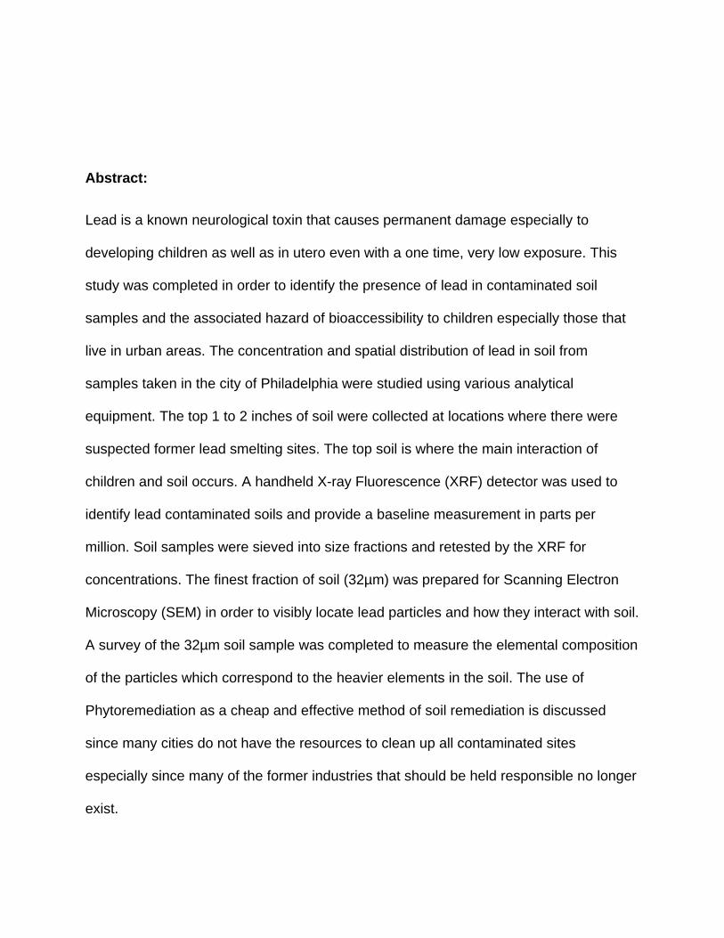
There are 36 former suspected lead smelting site within the city limits of

Philadelphia, all of which are no longer in operation. During the industrial revolution

there were many industries that were using lead, such as paint producers, and

contaminating the soils with gross quantities of lead due to the lack of environmental

laws and exposure limits. Lead was being introduced into urban soils from previous

industrial production, but now many of the areas where these industries existed are now

residential housing and neighborhoods. Lead has a very high adsorption rate (Kd) of

900 in soils which means that it stays attached to the soil and is not easily removed (PA

DEP). This means that soils that were contaminated in the mid 1900’s that contain lead

levels that exceed EPA and OSHA permissible exposure levels still are just as

contaminated today as when the industries were smelting lead (Thomas 1995).

Figure 1 (Above): A map of the city of Philadelphia and the suspected former lead

smelting sites throughout the city. Not all of the sites can be confirmed that they were

smelting lead due to the lack of laws on the reporting and restriction of the hazardous

metal. Locations with asterisks in the addresses are approximate locations since the

areas have been redeveloped and changed into residential neighborhoods since the

former industries have been removed. (Map Source: PA Bureau of Health Statistics and

Research, August 2004)

A third source of lead contamination in soils as well as residential houses is from

lead based paints as well as lead pipes used in the plumbing systems. Lead paint was

used in residential houses until 1978 when the U.S. Consumer Product Safety

Commission (CPSC) placed a final ban on it which prohibited the sales and use of lead

paint in homes. Most of the lead paint has been removed in residential houses, but even

after its removal lead can still be detected in high levels in dust in houses (Laidlaw

2011). Lead cannot exceed 40 micrograms in dust per square foot on the floors of a

house and lead cannot exceed 250 micrograms in the dust on window sills per square

foot (EPA 2001). Many houses that contained lead based paints have been remediated,

but there is another major source of lead contamination that children interact with such

as public parks and playgrounds.

Some of the areas in Philadelphia that were former suspected lead smelting sites

were located on or nearby areas that are currently public parks, playgrounds or schools.

In these locations the concentrations of lead can exceed the EPA limit which can be

hazardous to the health of children. The EPA exposure limit for lead concentrations in

bare soil in a yard is 1,200 ppm measured by average and only 400 ppm in children’s

play areas (EPA 2001). It is imperative that we determine the concentrations of lead that

are present in soil samples from urban areas. This is an especially important task in

order to remediate or remove lead from soils and reduce the amount of exposure to

urban populations, especially children which are more sensitive due to their on-going

neurological development.

Materials and Methods:

Soil samples were taken throughout the city of Philadelphia in areas that already

were suspected to have high levels of lead due to the former presence of suspected

lead smelting industries. Also soil samples were collected in areas that could be

hazardous to children or other individuals such as school yards and public playgrounds

in parks. A handheld X-ray fluorescence detector (Innov-X-Systems) was used to

determine the concentrations of lead at or near the surface of the soil. Once a location

tested positive for a high lead concentration, a shovel was used to remove the top 1 to 2

inches of soil. The soil sample was placed in a bag, labeled and brought back to the lab

for further processing and testing. A control sample was taken outside of the main door

of Merion Hall in West Chester, PA by the footpath that leads up to the stairs. For the

control sample the top inch of exposed soil was collected and tested by the handheld X-

ray Fluorescence detector. This control sample should not contain high levels of lead

unless there was a source of contamination on the soil. The control soil was never used

for lead smelting or processing and is located far enough away from a road that

combustion from leaded gasoline should not be present in the sample.

X-ray Fluorescence (XRF) is used for determining the bulk composition of a

sample, in this case soil, in a nondestructive manner (Shackley 2011). The X-ray

Fluorescence detector emits a concentrated X-ray beam that bombards the elements

that are present in the sample. The elements in the sample give off specific

wavelengths that correspond to their valence electron shells. The intensity of the

fluorescence X-rays that are emitted from the sample determines the concentrations of

the elements that are present (Kawai 1998). The readings of the concentrations are in

real time on the display screen on the device. These readings are used to determine the

level of contamination and are compared to the EPA standard which can be used to

determine if future steps are necessary for soil remediation.

Some of the samples were further processed after being collected in the field.

One specific sample, from Greensgrow Farm at 2501 East Cumberland St,

Philadelphia, PA 19125, is located only 300 feet away from a former suspected lead

smelting site. The Greensgrow Farm sample was collected the same way that the

others were, but in the lab the sample was sieved into four size fractions. The largest

fraction contained particles that are 2mm or larger, the next largest fraction contained

particles less than 2mm to 500 µm, the third fraction contained particles less than 500

µm to 250 µm and the smallest fraction contained particles less than 250 µm to 32 µm.

Each bag containing a fraction size was measured using the handheld XRF detector to

determine if there were differences in concentrations changed according to the size of

the soil particles. These samples were then compared to the whole soil control sample

that was taken outside of Merion Hall. The concentrations for each soil fraction size

were recorded and can be seen in Table 1 in the results section along with the other

samples used in this project.

Figure 2: Shows an aerial view of Greensgrow Farms in northeast Philadelphia along

East Cumberland Street. 2501 East Cumberland Street is the address for Greensgrow

Farms which is an urban farm and nursery. 2607 East Cumberland Street is a former

suspected lead smelting site. The proximity of the smelting site to the nursery/farm is

concerning since certain plants readily absorb lead from soil.

Once the concentrations of lead in the soil using the XRF were determined, the

next step was to prepare the soil fraction samples for the Scanning Electron Microscope

(SEM). A large pin stub mount used for the SEM and double side tape were used to

apply the soil samples to the stubs for the analysis. The soil samples were spread out

over the tape so that the particles were barely touching or not touching at all. The

spacing of particles is important for two reasons. The first is that if smaller soil particles

are being blocked by larger ones then the electron beam may not come into contact

with them unless a higher voltage across the filament is used. Secondly, X-ray

emissions that are being reported as a function of wavelength, which are specific to

elements that are emitted by particles, can be blocked by adjacent soil particles. This

can affect the reporting of the actual soil composition by Energy Dispersive

Spectroscopy (EDS) (Manceau 1996). In order to make the soil particles spread out so

that they could be applied to the stub, the soil was placed on a thin rubber sheet. A

small scoop of about 0.2 grams of the 32 µm soil fraction was weighed out using an

analytical scale on a piece of weigh paper. A hollow PVC tube was sanded down to

make the edges of the pipe as smooth as possible. Petroleum jelly was applied to the

sanded down tube which is used to decrease the friction of the rubber sheet against the

sanded down PVC tube. The rubber sheet was placed on top of the PVC tube, and the

soil was applied to the rubber sheet. The rubber sheet was then pulled and stretched

out over the pipe as tight as possible which effectively spread out the soil particles.

While holding the rubber sheet taunt with one hand, the other free hand could be used

to pick up the stub containing the double sided tape, and the stub was pressed against

the soil on the rubber sheet. This process allowed for wide spacing of the soil particles

for more accurate analysis using the SEM. For further information of the PVC tube

device that was used for this process; personal Communication: Dr. Ulrich Klabunde.

Scanning Electron Microscopy was used to determine the bulk composition of

soil particles, and also to determine possibly what the lead particles were binding to or

associated with. The prepared sample stub of spread out soil from above was loaded

into the SEM on a single position stage and the chamber was pumped using low

vacuum mode which has a pressure of around 75.0 to 100.0 Pascal. Once the chamber

reached the working pressure, the high voltage current was turned on to 20.00 kV and a

spot size of 5.0 was used for EDS analysis. Lead appears as brighter particles on the

electron microscope due to its heavy elemental weight. This is compared to the rest of

the soil particles’ composition which is much lighter elements in atomic weight and

therefore have a darker appearance on the SEM. After searching for particles on the

sample that appear much brighter than the main soil composition, EDS was completed

using the INCA software to determine the absorbance spectra of the particles. The

length of the particle sizes were measured from the SEM software using the scale bar.

A survey of the 32 µm sample from Greensgrow Farms in Philadelphia was run on the

SEM in order to provide the overall bulk composition of soil particles that were in the

same threshold region of brightness as the lead particles are. As an overall montage

image of the sample was completed to show what the sample looks like at a

magnification of 75x on the computer for the microscope.

Results:

The handheld XRF spectrometer gives the most accurate readings of the metals

present in soil samples. Table 1 shows the lead concentration results from the XRF

readings that were recorded. Three replicates were recorded for each sample, averaged

and standard deviations were calculated below. Each soil fraction size: >2mm, 500 µm,

250 µm and 32 µm, were measured separately from one another in order to determine if

and where the primary concentrations of lead are located in the soil. The results from

the three samples from the Greensgrow location varied slightly in lead concentrations,

but they are all above the EPA’s upper limit for children’s playgrounds. Sample 1 from

Greensgrow Farms contained the highest amounts of lead in the soil from the samples

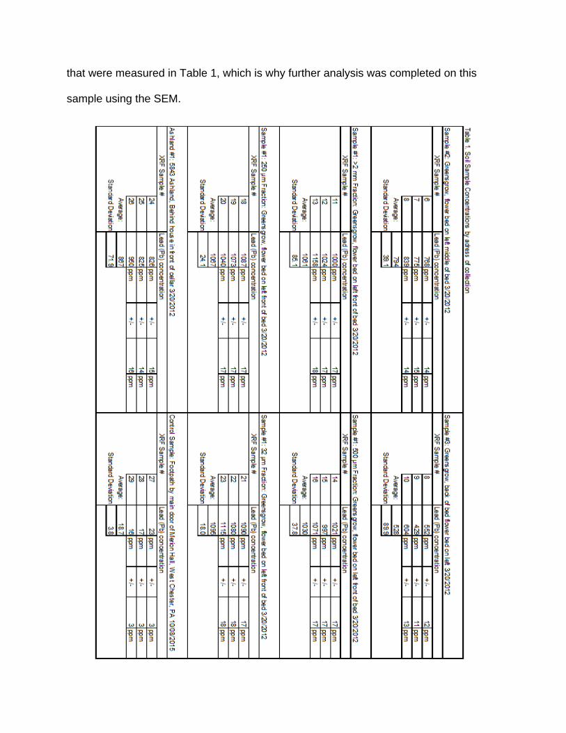
that were measured in Table 1, which is why further analysis was completed on this

sample using the SEM.

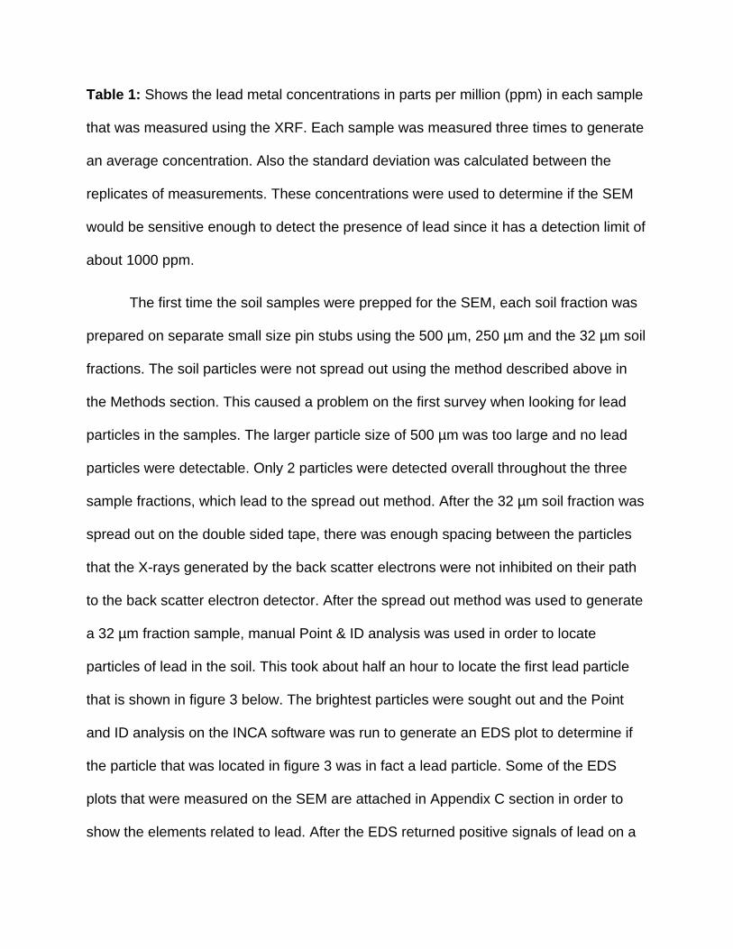
Table 1: Shows the lead metal concentrations in parts per million (ppm) in each sample

that was measured using the XRF. Each sample was measured three times to generate

an average concentration. Also the standard deviation was calculated between the

replicates of measurements. These concentrations were used to determine if the SEM

would be sensitive enough to detect the presence of lead since it has a detection limit of

about 1000 ppm.

The first time the soil samples were prepped for the SEM, each soil fraction was

prepared on separate small size pin stubs using the 500 µm, 250 µm and the 32 µm soil

fractions. The soil particles were not spread out using the method described above in

the Methods section. This caused a problem on the first survey when looking for lead

particles in the samples. The larger particle size of 500 µm was too large and no lead

particles were detectable. Only 2 particles were detected overall throughout the three

sample fractions, which lead to the spread out method. After the 32 µm soil fraction was

spread out on the double sided tape, there was enough spacing between the particles

that the X-rays generated by the back scatter electrons were not inhibited on their path

to the back scatter electron detector. After the spread out method was used to generate

a 32 µm fraction sample, manual Point & ID analysis was used in order to locate

particles of lead in the soil. This took about half an hour to locate the first lead particle

that is shown in figure 3 below. The brightest particles were sought out and the Point

and ID analysis on the INCA software was run to generate an EDS plot to determine if

the particle that was located in figure 3 was in fact a lead particle. Some of the EDS

plots that were measured on the SEM are attached in Appendix C section in order to

show the elements related to lead. After the EDS returned positive signals of lead on a

particle, a length measurement was taken which ranged in lengths from 1 µm to 20 µm.

The larger measurements usually occurred on the on the coated soil particles. Also,

particles are usually in the form of a lead oxide which makes determining the source of

the lead very difficult. More manual Point & ID analysis was completed in order to find

more lead particles and to obtain measurements of lead particle sizes.

Figure 3: The image above shows the first lead particle identified by Point & ID on the

INCA software. The length of the particle is shown above on the image in yellow which

is about 1.05 µm. The length of the particle was measured using the scale bar provided

in the bottom right corner of the image. This is one very small particle of many particles

that composes this aggregation of soil.

Spectrum In

stats. Mg Al Si P S Cl K Ca Ti Fe Pb O Total

Spectrum 1 Yes 0.9 10.2 16.5 4.69 0.52 1.61 0.97 2.64 18.7 43.3 100

Spectrum 2 Yes 0.63 9.14 14.1 1.97 1.55 0.88 2.87 20 12.1 36.8 100

Spectrum 3 Yes 0.69 9.97 15.7 0.68 3.79 1.62 1.16 3.1 20.7 42.6 100

All results in weight%

Table 2: This table shows the three spectrums that were taken of the particle that was

the first particle positively identified in the image above labeled as figure 3. After EDS

was completed using INCA software, a table of the results of the elements by weight

percentage was generated. The three spectrums were all measured on the brightest

particle on the image on figure 3, and spectrum 2 reported positive for peaks for lead.

12% of the total weight was lead on that particle.

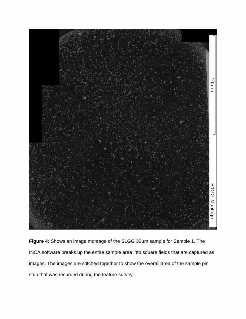
Figure 4: Shows an image montage of the S1GG 32µm sample for Sample 1. The

INCA software breaks up the entire sample area into square fields that are captured as

images. The images are stitched together to show the overall area of the sample pin

stub that was recorded during the feature survey.

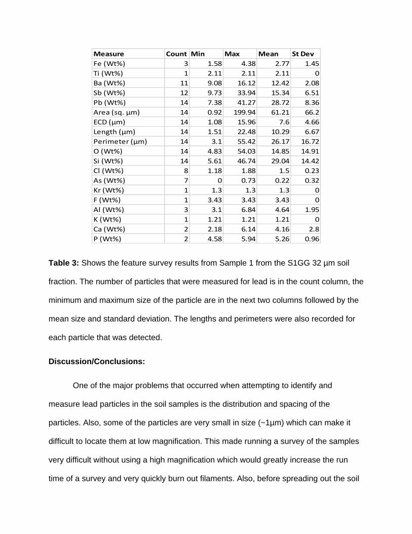
Table 3: Shows the feature survey results from Sample 1 from the S1GG 32 µm soil

fraction. The number of particles that were measured for lead is in the count column, the

minimum and maximum size of the particle are in the next two columns followed by the

mean size and standard deviation. The lengths and perimeters were also recorded for

each particle that was detected.

Discussion/Conclusions:

One of the major problems that occurred when attempting to identify and

measure lead particles in the soil samples is the distribution and spacing of the

particles. Also, some of the particles are very small in size (~1µm) which can make it

difficult to locate them at low magnification. This made running a survey of the samples

very difficult without using a high magnification which would greatly increase the run

time of a survey and very quickly burn out filaments. Also, before spreading out the soil

Measure Count Min Max Mean St Dev

Fe (Wt%) 3 1.58 4.38 2.77 1.45

Ti (Wt%) 1 2.11 2.11 2.11 0

Ba (Wt%) 11 9.08 16.12 12.42 2.08

Sb (Wt%) 12 9.73 33.94 15.34 6.51

Pb (Wt%) 14 7.38 41.27 28.72 8.36

Area (sq. µm) 14 0.92 199.94 61.21 66.2

ECD (µm) 14 1.08 15.96 7.6 4.66

Length (µm) 14 1.51 22.48 10.29 6.67

Perimeter (µm) 14 3.1 55.42 26.17 16.72

O (Wt%) 14 4.83 54.03 14.85 14.91

Si (Wt%) 14 5.61 46.74 29.04 14.42

Cl (Wt%) 8 1.18 1.88 1.5 0.23

As (Wt%) 7 0 0.73 0.22 0.32

Kr (Wt%) 1 1.3 1.3 1.3 0

F (Wt%) 1 3.43 3.43 3.43 0

Al (Wt%) 3 3.1 6.84 4.64 1.95

K (Wt%) 1 1.21 1.21 1.21 0

Ca (Wt%) 2 2.18 6.14 4.16 2.8

P (Wt%) 2 4.58 5.94 5.26 0.96

particles on the large sample stubs, the particles were too close in proximity to each

other. This may have caused an obstruction of the electron beam or the X-rays that are

emitted from the energy transfer of an electron moving from an outer valence electron

shell down to a lower energy shell. This is especially true in the larger soil fractions such

as the 500 µm and 250 µm samples. This is due to the fact that they have greater

topography due to the larger aggregates of soil packed together. The larger soil

fractions (500 µm) contained concentrations of lead in ppm that were similar in

concentrations to the smaller soil fraction size (<32 µm) which was confirmed by the

XRF results (Pyle 1996). It was very difficult to locate the small lead particles on the

surface of the large soil fraction particles because as the surface area of the particles

increases, the volume under the subsurface of the particles also increases. This means

that if there were lead particles present in the larger soil fractions, they are not visible

using imaging on the SEM and random point and ID analysis would have been as

efficient as finding a needle in a haystack. Due to these issues, the spread out method

of the smallest soil fraction (32 µm) as described above in the Materials & Methods

section was developed. The smaller particles contain a greater surface to volume ratio,

which means that the probability that a lead particle is present on surface is much

higher. Lead particle sizes in these samples ranged from smaller than 1µm to up to

20µm, so in order to find those very small particles the smaller soil fraction is more

desirable than the larger fractions. The larger size pin stubs were used instead of the

smaller size pin stubs, because the larger pin stubs allow more soil to be loaded over a

larger area. This increased the potential number of lead particles and made them easier

to find at a lower magnification. Also, the spacing between the particles on the spread

out method allowed for the X-rays to reach the back scatter electron detector much

easier without obstruction from other soil particles.

Since lead is a much heavier element than the primary comprising elements

normally present in soil, they tend to be much brighter in comparison which is an

advantage. The contrast setting was increased to a value around 80 and the brightness

was turned down to a value around 15. This gave the heavy elements higher contrast

so that when the brightness was turned down, the heavy elements such as lead were

the only particles that were still showing up on the microscope. This helped to locate the

lead particles in a shorter amount of time. Also the contrast settings could be used to

calibrate the SEM to find only heavy elements so that there were less particles to be

analyzed during a survey run; this reduced the survey run times.

Using the smallest soil fraction size of <32 µm is potentially a very important soil

fraction when it comes to how humans, especially children, may become exposed to

lead contaminated soils. Soil samples that are less than 32 µm are more readily

available to become airborne and end up in our lungs and ultimately enter the

bloodstream. The lead particles that are only 1 µm in length are of primary concern

since these smaller particles can enter the respiratory or digestive systems more easily

and can be absorbed into the blood which can affect the nervous system (Clarkson

1987). Lead particles that are 10 µm or less in size are very susceptible to entering our

bloodstream once those soil particles enter the airways and lungs (Boisa 2014). The

movement of lead from a source to soil, soil which is crushed to dust, dust which can

become airborne and absorb into the bloodstream via the lungs is caused by industrial

sources, leaded gasoline exhaust and pulverized lead particles in soil (Mamane 1995).

There are many factors that can affect the amount of exposure in children which

include: season of the year, weather which includes wind, age, socioeconomic status,

and time spent outside (Mielke 1998). Children who live in old industrial cities and do

not have much wealth cannot not afford to move to a new home that has better soil

quality without lead contamination. This can cause many exposures throughout their

childhood either via digestion or inhalation during their critical neurological development

stages (Garcia-Rico 2015).

Lead can enter the bloodstream via digestion from contaminated soils when

hands are not adequately washed after exposure. This is especially true in young

children who are not concerned with washing their hands before eating or putting their

hands in their mouths especially after playing in the dirt and soil. Children play in the dirt

which is normally seen as harmless in areas where lead concentrations are below 400

ppm, but this can be extremely hazardous to neurological development even after a one

time small exposure (Mendelsohn 1998). The standard set by the World Health

Organization (WHO) for the action level of lead in children’s blood is 10 µg/dl, but

studies have shown that in children that have had blood lead levels below 10 µg/dl for a

lifetime still have neurological damage (Koller 2004). In a simulated stomach digestion

study in Glasgow Scotland, which used a pH of 1.5 to simulate the conditions in our

stomach, the study determined that a range of 23-77% of the lead in contaminated soils

could be bioaccessible to humans (Farmer 2011).

Locating areas in cities where children may become exposed to elevated lead

levels in soil is important in order to reduce the possibility of exposure of any

concentration of lead to children. Figure 5 below shows an example in Philadelphia

where soil studies should be completed in order to determine the lead concentrations of

an industrial reclaimed plot of land which is now a public space. Figure 5 shows a

Google Earth satellite image of Chew Park which is located along Washington Avenue

between South 18th and 19th streets. This area has been reclaimed and converted into a

public park which contains playgrounds for children, a baseball diamond and other play

areas which from this aerial image appears that much of the surface of the park is

exposed soil. This location also is one of the former suspected lead smelting sites in the

city of Philadelphia that can be found on Figure 1 much like Greensgrow Farms in

northeast Philadelphia. This should raise an alarm to residents who use this park that

there could be elevated lead levels in the soil. Since this is a potential source of

exposure to young children, samples should be taken here by the city or state and

remediation steps should be taken if the concentrations are above the WHO’s standards

in order to reduce lead blood levels of children in Philadelphia. Further research should

be completed of all parks, playground areas, schools and anywhere else children are

regularly exposed to dirt. This should especially be done in areas where former

industries may have been used in lead production (Eckel 2001).

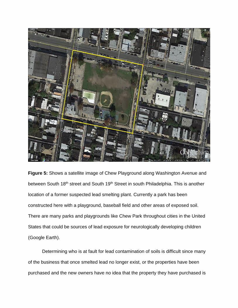
Figure 5: Shows a satellite image of Chew Playground along Washington Avenue and

between South 18th street and South 19th Street in south Philadelphia. This is another

location of a former suspected lead smelting plant. Currently a park has been

constructed here with a playground, baseball field and other areas of exposed soil.

There are many parks and playgrounds like Chew Park throughout cities in the United

States that could be sources of lead exposure for neurologically developing children

(Google Earth).

Determining who is at fault for lead contamination of soils is difficult since many

of the business that once smelted lead no longer exist, or the properties have been

purchased and the new owners have no idea that the property they have purchased is

heavily contaminated with lead. Also expecting the city or state to pay for soil

remediation is not possible since many cities and states have budget issues and simply

cannot afford to hire remediation companies. Finding other, cheaper methods of

remediation is very important in order to start the remediation process right away

without generating a large remediation cost. This is why phytoremediation could be an

effective method of treatment of contaminated soil since it is a cheap and easy to grow

heavy metal absorbing plants, cut them down and treat the plants as hazardous waste

instead of removing and treating enormous amounts of contaminated soil.

Phytoremediation is an easy and cost effective method for remediating lead

contaminated soil. Plants that absorb lead usually only absorb about 1% of lead in their

biomass, but with the addition of chelating agents such as Ethylenediaminetetraacetic

acid (EDTA) lead absorption can be increased from the roots of the plants to the shoots

by up to 120 fold (Huang 1997). While lead is not an essential element for the

functionality of plant systems it can be absorbed into the root systems, which makes

certain vegetable skins such as carrots or potatoes more susceptible to being

contaminated with lead (Pourrut 2011). Lead is not considered to generally be a

phytotoxic compound to plants which is beneficial for plant use to absorb and collect

lead for soil remediation (Stevens 2003).

Continuing to locate urban soils that are contaminated with lead throughout the

United States as well as the world is very important in order to protect the neurological

development of the children who come into contact with these soils on a semi-daily

basis. Ongoing sample collection and analysis must be done in areas that are near

highways or used to house lead smelting industries in order to keep lead sensitive

children away and healthy (Motto 1970). Profiling of where lead is located in soil and

finding the other elements that are associated with lead can help to identify the sources

of lead contamination as well as give in sight towards the bioaccessibility to humans.

Cheap and effective lead remediation methods for soil must be invented in order to

clean up our post-industrial revolution world that we live in.

Bibliography:

Alkorta, I., J. Hernández-Allica, J.m. Becerril, I. Amezaga, I. Albizu, and C. Garbisu.

"Recent Findings on the Phytoremediation of Soils Contaminated with Environmentally Toxic Heavy Metals and Metalloids Such as Zinc, Cadmium, Lead, and Arsenic." Reviews in Environmental Science and Bio/Technology Re/Views in Environmental Science and Bio/Technology 3, no. 1 (2004): 71-90.

Boisa, Ndokiari, Nwabueze Elom, John R. Dean, Michael E. Deary, Graham Bird, and

Jane A. Entwistle. "Development and Application of an Inhalation Bioaccessibility Method (IBM) for Lead in the PM10 Size Fraction of Soil." Environment International 70 (2014): 132-42.

Brugge, Doug, John L Durant, and Christine Rioux. "Near-highway Pollutants in Motor

Vehicle Exhaust: A Review of Epidemiologic Evidence of Cardiac and Pulmonary Health Risks." Environmental Health Environ Health 6, no. 23 (2007).

Clarkson, T W. "Metal Toxicity in the Central Nervous System." Environ Health Perspect Environmental Health Perspectives 75 (1987): 59-64.

Eckel, William P., Rabinowitz, Michael B., and Foster, Gregory D. (April 2001). Discovering Unrecognized Lead-Smelting Sites by Historical Methods, American Journal of Public Health, 91, (4), 625-627.

"Environmental Health and Medicine Education." Lead (Pb) Toxicity: Key Concepts.

August 20, 2007. Accessed October 5, 2015.

http://www.atsdr.cdc.gov/csem/csem.asp?csem=7&po=8.

EPA "Lead; Identification of Dangerous Levels of Lead." Federal Register 66, no. 4

(2001): 1-35.

Farmer, John G., Andrew Broadway, Mark R. Cave, Joanna Wragg, Fiona M. Fordyce,

Margaret C. Graham, Bryne T. Ngwenya, and Richard J.f. Bewley. "A Lead

Isotopic Study of the Human Bioaccessibility of Lead in Urban Soils from

Glasgow, Scotland." Science of the Total Environment 406, no. 23 (2011): 4958-

965.

García-Rico, Leticia, Diana Meza-Figueroa, A. Jay Gandolfi, Rafael Del Río-Salas,

Francisco M. Romero, and Maria Mercedes Meza-Montenegro. "Dust–Metal

Sources in an Urbanized Arid Zone: Implications for Health-Risk Assessments."

Arch Environ Contam Toxicol Archives of Environmental Contamination and

Toxicology, 2015.

Gidlow, D. A. "Lead Toxicity." Occupational Medicine 54, no. 2 (2004): 76-81.

Gulson, B., J. Davis, K. Mizon, M. Korsch, and J. Bawdensmith. "Sources of Lead in

Soil and Dust and the Use of Dust Fallout as a Sampling Medium." Science of

The Total Environment 166, no. 1-3 (1995): 245-62.

Huang, Jianwei W., Jianjun Chen, William R. Berti, and Scott D. Cunningham.

"Phytoremediation of Lead-Contaminated Soils: Role of Synthetic Chelates in

Lead Phytoextraction." Environmental Science & Technology Environ. Sci.

Technol. 31, no. 3 (1997): 800-05.

Hurst, Richard W., Terry E. Davis, and Barbara D. Chinn. "Peer Reviewed: The Lead

Fingerprints of Gasoline Contamination." Environmental Science & Technology

Environ. Sci. Technol. 30, no. 7 (2011): 304–307.

Kawai, Jun, Kouichi Hayashi, Kazuaki Okuda, and Atsushi Nisawa. "X-Ray Absorption

Spectroscopy Using X-Ray Fluorescence Spectrometer." The Rigaku Journal 15,

no. 2 (1998): 33-37.

Koller, Karin, Terry Brown, Anne Spurgeon, and Len Levy. "Recent Developments in

Low-Level Lead Exposure and Intellectual Impairment in Children." Environ

Health Perspect Environmental Health Perspectives 112, no. 9 (2004): 987-94.

Laidlaw, Mark A.s., and Mark P. Taylor. "Potential for Childhood Lead Poisoning in the

Inner Cities of Australia Due to Exposure to Lead in Soil Dust." Environmental

Pollution 159 (2011): 1-9.

Manceau, Alain, Marie-Claire Boisset, Géraldine Sarret, Jean-Louis Hazemann, Michel

Mench, Philippe Cambier, and René Prost. "Direct Determination of Lead

Speciation in Contaminated Soils by EXAFS Spectroscopy." Environmental

Science & Technology Environ. Sci. Technol. 30, no. 5 (1996): 1540-552.

Mendelsohn, A. L., B. P. Dreyer, A. H. Fierman, C. M. Rosen, L. A. Legano, H. A.

Kruger, S. W. Lim, and C. D. Courtlandt. "Low-Level Lead Exposure and

Behavior in Early Childhood." Pediatrics 101, no. 3 (1998).

Motto, Harry, Robert, Daines, Daniel M. Chilko, and Carlotta K. Motto. "Lead in Soils

and Plants: Its Relation to Traffic Volume and Proximity to Highways."

Environmental Science & Technology Environ no. 3 (1970): 231-37.

Mamane, Y., Rd Willis, Rk Stevens, and Jl Miller. "Scanning Electron Microscopy/X-Ray

Fluorescence Characterization of Lead-Rich Post-Abatement Dust." Lead in

Paint, Soil and Dust: Health Risks, Exposure Studies, Control Measures,

Measurement Methods, and Quality Assurance, 1995.

Mielke, Howard W., and Patrick L. Reagan. "Soil Is an Important Pathway of Human

Lead Exposure." Environmental Health Perspectives 106 (1998): 217-29.

Pourrut, Bertrand, Muhammad Shahid, Camille Dumat, Peter Winterton, and Eric Pinelli.

"Lead Uptake, Toxicity, and Detoxification in Plants." Reviews of Environmental

Contamination and Toxicology Reviews of Environmental Contamination and

Toxicology Volume 213 213 (2011): 113-36.

Pyle, Steven M., John M. Nocerino, Stanley N. Deming, John A. Palasota, Josephine M.

Palasota, Eric L. Miller, Daniel C. Hillman, Conrad A. Kuharic, William H. Cole,

Patricia M. Fitzpatrick, Michael A. Watson, and Ky D. Nichols. "Comparison of

AAS, ICP-AES, PSA, and XRF in Determining Lead and Cadmium in Soil."

Environmental Science & Technology Environ. Sci. Technol. 30, no. 1 (1996):

204-13.

Ruby, M. V., R. Schoof, W. Brattin, M. Goldade, G. Post, M. Harnois, D. E. Mosby, S.

W. Casteel, W. Berti, M. Carpenter, D. Edwards, D. Cragin, and W. Chappell.

"Advances in Evaluating the Oral Bioavailability of Inorganics in Soil for Use in

Human Health Risk Assessment." Environmental Science & Technology Environ.

Sci. Technol. 33, no. 21 (1999): 3697-705.

Senut, Marie-Claude, Pablo Cingolani, Arko Sen, Adele Kruger, Asra Shaik, Helmut

Hirsch, Steven T Suhr, and Douglas Ruden. "Epigenetics of Early-life Lead

Exposure and Effects on Brain Development." Epigenomics, 2013, 665-74.

Shackley, M. Steven. "An Introduction to X-Ray Fluorescence (XRF) Analysis in

Archaeology." In X-ray Fluorescence Spectrometry (XRF) in Geoarchaeology, 7-

44. New York: Springer, 2011.

"Statewide Health Standards." Pennsylvania Department of Environmental Protection.

Accessed October 17, 2015.

http://www.portal.state.pa.us/portal/server.pt/community/standards,_guidance_an

d_procedures/21543/statewide_health_standards/1034862.

Stevens, Daryl P., Mike J. Mclaughlin, and Tundi Heinrich. "Determining Toxicity Of

Lead And Zinc Runoff In Soils: Salinity Effects On Metal Partitioning And On

Phytotoxicity." Environmental Toxicology and Chemistry Environ Toxicol Chem

22, no. 12 (2003): 3017-024.

"Suspected Former Lead Smelter Sites: A Potential Risk Factor for Childhood Lead

Poisoning." August 1, 2004. Accessed October 5, 2015.

www.health.pa.gov/migration/Documents/smelterfactsheetandmaps_pdf.

Thomas, V. "The Elimination of Lead in Gasoline." Annual Review of Energy and the

Environment 20 (1995): 301-24.

Appendix A:

Soil Preparation Protocol for Scanning Electron Microscope

Materials:

Handheld X-Ray Fluorescence (XRF) Detector

Collected soil samples in plastic bags

Analytical scale

Weighing spatula

Weighing paper

PVC pipe

Petroleum Jelly

Rubber Sheet

Double sided clear tape

Large Sample Pin Stubs

Scalpel

Fine point lab marker

Protocol:

1. Use the handheld X-Ray Fluorescence detector on the plastic bagged sample of

soil in order to get the concentration of the metals in the soil sample.

2. Sieve the soil samples into the desired fractions sizes (ex: 2 mm, 500 µm, 250

µm, and 32 µm) and place the fractions into separate plastic ziploc bags.

3. Use the handheld X-Ray Fluorescence detector on the bagged samples of soil

for each fraction and record the results to detect if the concentrations of the

metals vary by fraction size.

4. Use the smallest sized fraction of soil (ie: 32 µm) and weight out 0.2 grams of the

soil on a weighing paper.

5. Transfer the soil from the weighing paper onto the middle of the thin rubber

sheet.

6. Apply some petroleum jelly around the sanded top edge of the PVC pipe in order

to reduce friction.

7. Cut off a piece of double sided tape so that the majority of a large sample pin

stub has tape on it (you do not have the cover the whole stub).

8. Use the scalpel to cut off the excess tape so that the tape has rounded edges

and weigh the pin stub on the scale.

9. Place the rubber sheet on top of the PVC pipe and spread it out into a thin,

uniform surface coating on the rubber sheet.

10. Stretch the rubber sheet with the soil on it outward in all directions over the PVC

pipe in order to spread out the soil particles so that they are barely touching one

another.

11. Once the soil particles are thoroughly spread out, hold the stretched out rubber

with one hand around the sides of the pipe and pick up the sample stub with your

other hand and press the prepared sample stub on to the spread out soil

particles on the rubber. (you are aiming to have a thinly coated piece of tape with

soil particles so that it is fairly hard to see them with the naked eye)

12. Weigh the pin stub again on the scale to see how much soil by weight was

applied to the pin stub.

13. Use the handheld XRF detector on the pin stub with the soil on it to ensure that

the sample is still reading about the same concentration of lead as the full bag of

soil fraction size that you are working with (ie: 32 µm).

14. The sample is now ready for analysis using the Scanning Electron Microscope. A

carbon coating can be applied to the sample to prevent charging on the SEM if

you are having this issue.

15. Store the prepared sample pin stub in a covered container so that dust does not

contaminate the sample by sticking on the double sided tape.

Appendix B:

Energy Dispersive Spectrometry Analysis (EDS) Using Point & ID on the

Scanning Electron Microscope

Materials:

Prepared Large Sample Pin Stubs

Scanning Electron Microscope

INCA Software

Microsoft Word

Protocol:

1. Load the prepared soil sample on the single stage holder in the chamber of the

Scanning Electron Microscope.

2. Click on the low vacuum radial button on the right computer monitor with the

microscope controls.

3. The computer will prompt you to flip the lever to the low vacuum setting if it is not

already in the correct position (the lever is located above the square sample

chamber of the microscope to the left)

4. Wait until the vacuum has pumped down to the operating pressure and the

vacuum square in the bottom right of the screen will turn green showing that the

chamber is at the operational level.

5. Use the mouse to raise the stage to the 10mm line by clicking and holding in the

mouse scroll wheel and dragging the mouse upwards. Once you are in position

let go of the mouse wheel and the stage will stop moving.

6. Change the detector of the upper left hand quadrant to the Solid State detector

which is the Back Scatter Detector for low vacuum analysis.

7. Click on the HV button on the right side of the microscope controls in order to

turn the high voltage on to the filament which turns on the electron beam. Make

sure that the beam current is operating at 100 µA if not change it by

increasing/decreasing the bias by un-checking the auto bias button.

8. Move around the sample in order to find an area of interest by double left clicking

on the screen. If you are looking for a heavy element such as lead then adjust

the contrast to around 75 and a brightness setting of around 20. This will allow

the heaviest elements to still show up on the microscope while other elements

will disappear.

9. Open the INCA software on the left computer and make sure that the drop down

menu in the bottom left has “Point & ID” selected.

10. Use the flow chart on the left hand side of the software in order to name the

project file and then the sample name on the next point downwards of the flow

chart.

11. Move left on the flow chart to microscope setup. Click the green circle with the

red arrows going around it to start cyclic acquisition and determine which

element has the strongest peak.

12. Click the next square down to Quant Optimization and use the element from

microscope setup in the drop down menu and click the green circle in the upper

right hand side of the screen to optimize your measurements. Once it is finished

click the measure button and make sure that it says OK.

13. Next move to the right to the area of interest button on the INCA software and

make sure that the back scatter detector box is clicked on in the upper center of

the selection buttons. Click the green capture button when you have your image

that you want to analyze on the right computer monitor with the microscope

controls.

14. Once the image is captured, then move down to the next flow chart button which

is Acquire Spectra. Click the left mouse button to select areas on the image that

you want to run Energy Dispersive Spectrometry (EDS) on and once you have all

the areas selected, wait for the software to finish all the sample locations.

15. Move down to the Confirm Elements button which is where you can add or

remove elements that do not typically appear in your samples if they share a

similar peak with another element.

16. Move down to Quant on the flow chart which is where a chart for the elements

present in the EDS are listed by atomic and weight percentage.

17. Finally click on Report below Quant and you can export a Word document so you

can access your data on another computer. Put the files on a flash drive so you

can take them away from the computer.

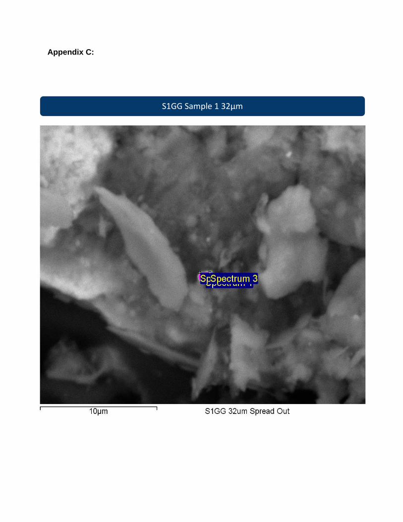
Appendix C:

S1GG Sample 1 32µm

10/27/2015 3:59:44 PM

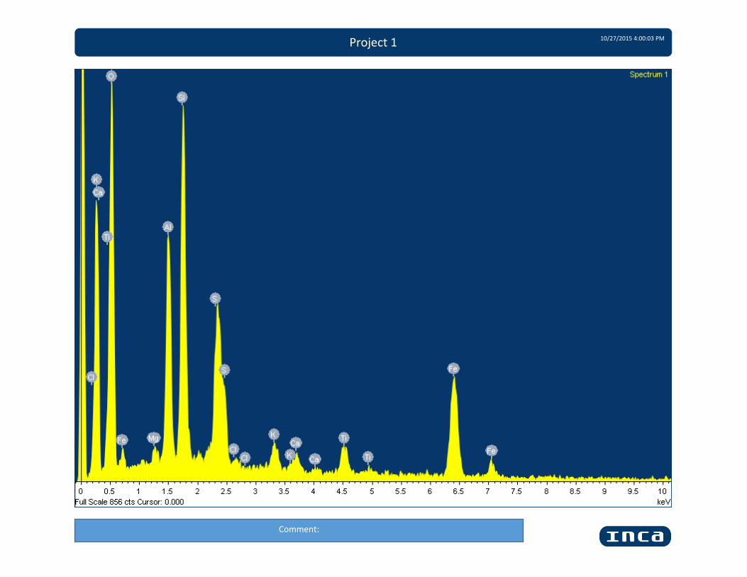
Project 1 10/27/2015 4:00:03 PM

Comment:

Project 1 10/27/2015 4:00:06 PM

Comment:

Project 1 10/27/2015 4:00:09 PM

Comment:

Project 1 10/27/2015 4:00:23 PM

Comment:

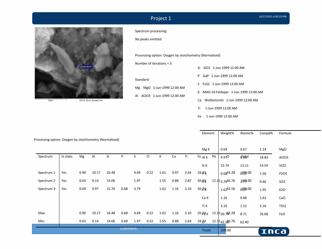
Spectrum processing:

No peaks omitted

Processing option: Oxygen by stoichiometry (Normalised)

Number of iterations = 3

Standard:

Mg MgO 1-Jun-1999 12:00 AM

Al Al2O3 1-Jun-1999 12:00 AM

Si SiO2 1-Jun-1999 12:00 AM

P GaP 1-Jun-1999 12:00 AM

S FeS2 1-Jun-1999 12:00 AM

K MAD-10 Feldspar 1-Jun-1999 12:00 AM

Ca Wollastonite 1-Jun-1999 12:00 AM

Ti 1-Jun-1999 12:00 AM

Fe 1-Jun-1999 12:00 AM

Element Weight% Atomic% Compd% Formula

Mg K 0.69 0.67 1.14 MgO

Al K 9.97 8.66 18.83 Al2O3

Si K 15.70 13.11 33.59 SiO2

P K 0.68 0.51 1.56 P2O5

S K 3.79 2.77 9.46 SO3

K K 1.62 0.97 1.95 K2O

Ca K 1.16 0.68 1.62 CaO

Ti K 3.10 1.52 5.16 TiO2

Fe K 20.74 8.71 26.68 FeO

O 42.56 62.40

Totals 100.00

Processing option: Oxygen by stoichiometry (Normalised)

Spectrum In stats. Mg Al Si P S Cl K Ca Ti Fe Pb O Total

Spectrum 1 Yes 0.90 10.17 16.48 4.69 0.52 1.61 0.97 2.64 18.73 43.28 100.00

Spectrum 2 Yes 0.63 9.14 14.06 1.97 1.55 0.88 2.87 20.03 12.11 36.76 100.00

Spectrum 3 Yes 0.69 9.97 15.70 0.68 3.79 1.62 1.16 3.10 20.74 42.56 100.00

Max. 0.90 10.17 16.48 0.68 4.69 0.52 1.62 1.16 3.10 20.74 12.11 43.28

Min. 0.63 9.14 14.06 0.68 1.97 0.52 1.55 0.88 2.64 18.73 12.11 36.76

All results in weight%

Martin 36