development and use of water quality indices (wqi) to

DEVELOPMENT AND USE OF WATER QUALITY INDICES (WQI) TO

ASSESS THE IMPACT OF BMP IMPLEMENTATION ON WATER QUALITY

IN THE COOL RUN TRIBUTARY OF THE WHITE CLAY CREEK

WATERSHED

by

Alison Kiliszek

A thesis submitted to the Faculty of the University of Delaware in partial fulfillment of the requirements for the degree of Master of Science in Bioresources Engineering

Spring 2010

Copyright 2010 Alison Kiliszek All Rights Reserved

DEVELOPMENT AND USE OF WATER QUALITY INDICES (WQI) TO

ASSESS THE IMPACT OF BMP IMPLEMENTATION ON WATER QUALITY

IN THE COOL RUN TRIBUTARY OF THE WHITE CLAY CREEK

WATERSHED

by

Alison Kiliszek

Approved: __________________________________________________________ Anastasia E. M. Chirnside, Ph.D. Professor in charge of thesis on behalf of the Advisory Committee Approved: __________________________________________________________ William Ritter, Ph.D. Chair of the Department of Bioresources Engineering Approved: __________________________________________________________ Robin Morgan, Ph.D. Dean of the College of Agricultural and Natural Resources Approved: __________________________________________________________ Debra Hess Norris, M.S. Vice Provost for Academic and International Programs

iii

ACKNOWLEDGMENTS

This research report was prepared by Alison Kiliszek to fulfill the

requirements by the University of Delaware for a degree of Master in Bioresources

Engineering. Many thanks go to Dr. Anastasia Chirnside for being my academic

advisor and always providing me with words of encouragement and support. I also

wish to thank Soraya Azahari, Nicole Dobbs, Drew Erensel, Miles Fisher, Kaitlin

Green, Ryan Minor, Lauren Popyack, and Nicole Scarborough for helping in the

sample collection and analysis. Special thanks to my family and friends who

supported and encouraged me throughout the years.

Anastasia Chirnside thought of the concept of a Water Quality Index

(WQI) for the UD Experimental Watershed to aid the college in determining the

effects of the implemented Best Management Practices (BMPs). She started to

research previously created WQIs as a staring point to the project that has evolved into

a working model for the future. We hope the University of Delaware continues to

monitor the Cool Run stream to provide an on-campus education and research site that

will show faculty, staff, and students the effects and importance of BMPs.

iv

TABLE OF CONTENTS

ACKNOWLEDGMENTS ............................................................................................. iii LIST OF TABLES ......................................................................................................... vi LIST OF FIGURES ..................................................................................................... viii ACRONYMS AND ABBREVIATIONS .................................................................... xiii ABSTRACT ................................................................................................................. xv Chapter 1 WATER QUALITY INDICES: ASSESSING STREAM HEALTH ................. 1

Introduction ........................................................................................................ 1 Objectives ........................................................................................................... 5 Literature Review ............................................................................................... 6

2 METHODS ....................................................................................................... 17 Characterization of Monitoring Program ......................................................... 17 Site Description ................................................................................................ 18

Sampling Site 1 ....................................................................................... 29 Sampling Site 2 ....................................................................................... 30 Sampling Site 3 ....................................................................................... 31 Sampling Site 4 ....................................................................................... 32 Sampling Site 5 ....................................................................................... 33 Sampling Site 6 ....................................................................................... 34 Sampling Site 7 ....................................................................................... 35 Sampling Site 8 ....................................................................................... 36

Characterization of Best Management Practices .............................................. 37 Constructed Wetlands .............................................................................. 39 Gore Hall Wetlands Floodplain and Weir ............................................... 41 Livestock Exclusion - Fencing of Streams .............................................. 43 Manure Collection System ...................................................................... 43 Riparian Buffer Zones ............................................................................. 45 Small Pond .............................................................................................. 47

Delaware Standards, Delaware Criteria and EPA Water Quality Criteria........ 50 Calculation of Subindices ................................................................................. 55

Uniformly Decreasing Subindices ........................................................... 56

v

Nonuniformly Decreasing Subindices ..................................................... 57 Unimodal Subindices .............................................................................. 58 Overall Water Quality Index ................................................................... 59

Model Development ......................................................................................... 60 WQI Calculation ...................................................................................... 60 Model Validation ..................................................................................... 62

Assessment of BMP Efficiency ........................................................................ 62

3 RESULTS AND DISCUSSION ....................................................................... 65 Determination of Subindex Equation Constants .............................................. 70 Comparison of Determined Constants .............................................................. 72 Comparison of the Sub-KWQI to Water Quality Parameter

Concentration .......................................................................................... 76 Model Development ....................................................................................... 100

Model Overview .................................................................................... 101 Model Options ....................................................................................... 103 Model Example ..................................................................................... 104 Model Design Assessment: Comparing Kiliszek WQI Ratings to

Harrell (2002) Grading Scale .................................................... 119 Selection of Parameter Sets for KQWI Model Assessments ................. 126

Cool Run KWQI Model Assessments ............................................................ 136 Analysis of Changes between 2001 and 2009 (Sites 2, 3, 4 and 5) ....... 136 Analysis of Gore Hall Wetland (Sites 1, 2, 3 and 4) ............................. 140 Analysis of Riparian Buffer Zone between Sites 2 and 6 ...................... 145 Analysis of Riparian Buffer Zone and Pond (Sites 5 and 6) ................. 150 Analysis of Manure Collection System (Site 8) .................................... 152 Analysis of UD Farm (Standards and Criteria Approach) ..................... 155 Analysis of UD Farm (BMP Approach) ................................................ 169

4 CONCLUSIONS AND FUTURE GOALS .................................................... 172 REFERENCES ........................................................................................................... 175

vi

LIST OF TABLES

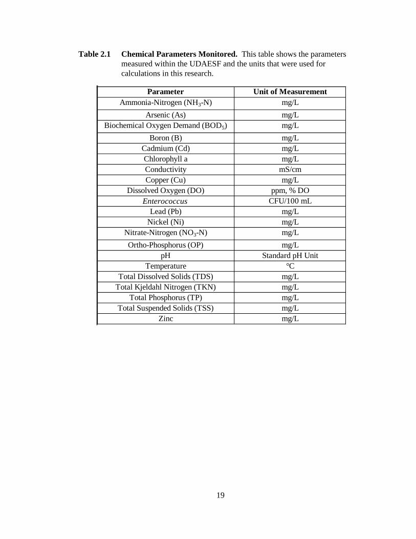
Table 2.1 Chemical Parameters Monitored ............................................................. 19

Table 2.2 Analytical Methods .................................................................................. 20

Table 2.3 Base Flow Summary ................................................................................ 21

Table 2.4 Storm Flow Summary .............................................................................. 21

Table 2.5 BMP Summary. ....................................................................................... 39

Table 2.6 General Delaware Fresh Water Quality Standards .................................. 51

Table 2.7 Delaware Water Quality Criteria for Aquatic Life Protection ................. 52

Table 2.8 Delaware Water Quality Criteria for Human Health Protection .............. 53

Table 2.9 EPA Ecoregional Nutrient Water Quality Criteria .................................. 53

Table 2.10 EPA “Gold Book” Criteria ...................................................................... 54

Table 2.11 EPA Region 7 4B Rationale .................................................................... 54

Table 2.12 EPA Volunteer Stream Monitoring Manual ............................................ 55

Table 3.1 Average Annual Concentrations of Monitored Water Quality Parameters- 2006 ..................................................................................... 66




Table 3.5 Nonuniformal Subindex qT Constants ..................................................... 73

Table 3.6 Uniform Subindex Constants .................................................................. 74

vii

Table 3.7 Unimodal Subindex Constants ................................................................ 76

Table 3.8 Table of Options built into Model ......................................................... 104

Table 3.9 Rating Range Guides for Harrell (2002) and Kiliszek WQI ................. 120

Table 3.10 Parameter Scoring Guides for Harrell (2002) and Kiliszek WQI .......... 121

Table 3.11 Kiliszek WQI vs Harrell (2002) Grading System .................................. 123

Table 3.12 Parameter Sets ....................................................................................... 128

Table 3.13 Sub-KWQI Using Average 2009 Data from Site 4 ............................... 132

Table 3.14 Parameter Set WQI Value ..................................................................... 133

Table 3.15 2001 and 2009 Sub-KWQI Values for Sites 2, 3, 4, and 5 .................... 137

Table 3.16 2001 and 2009 KWQI Values for Sites 2, 3, 4 and 5 ............................ 138

Table 3.17 Percent Change between 2001 and 2009 Quality Variables .................. 138

Table 3.18 Wetland Analysis and Parameter Set Comparison ................................ 141

Table 3.19 Actual and Estimated sub-KWQI for Site 2 (General Wetland) ........... 142

Table 3.20 Actual and Estimated sub-KWQI for Site 2 (DWQS +DWQCPAL) .... 142

Table 3.21 Actual and Estimated KWQI for Site 2 ................................................. 144

Table 3.22 Sub-KWQI Values Using Minimum Riparian Buffer Zone Set. ........... 146

Table 3.23 Sub-KWQI Values Using General Riparian Buffer Zone Set ............... 148

Table 3.24 Sub-KWQI Values Using Minimum Riparian Buffer Zone and Pond Set.. ............................................................................................... 151

viii

LIST OF FIGURES

Figure 2.1 Delaware River Basin ............................................................................. 23

Figure 2.2 White Clay Creek Watershed ................................................................. 24

Figure 2.3 The University of Delaware Experimental Watershed ........................... 25

Figure 2.4 Newark Research and Education Center of the University of Delaware College of Agriculture and Natural Resources – West side of UDAESF ..................................................................................... 26

Figure 2.5 Newark Research and Education Center of the University of Delaware College of Agriculture and Natural Resources – East side of UDAESF ..................................................................................... 26

Figure 2.6 Sample Site Location in the UD Experimental Watershed .................... 27

Figure 2.7 Sample Site Locations in UD Experimental Watershed – West side of NRECF ....................................................................................... 28

Figure 2.8 Sample Site Locations in UD Experimental Watershed – East side of NRECF ............................................................................................... 28

Figure 2.9 UDAESF Site 1 ...................................................................................... 29








Figure 2.17 BMP Locations on the Newark Research and Education Farm ............. 38

Figure 2.18 BMP Locations on the Newark Research and Education Farm ............. 38

Figure 2.19 Constructed Wetland .............................................................................. 40

ix

Figure 2.20 Gore Hall Wetland.................................................................................. 42

Figure 2.21 Gore Hall Weir ....................................................................................... 42

Figure 2.22 Fencing of Streams ................................................................................. 43

Figure 2.23 Manure Collection System ..................................................................... 44

Figure 2.24 Poorly Maintained Riparian Buffer Zone ............................................... 46

Figure 2.25 Adequately Maintained Riparian Buffer Zone ....................................... 47

Figure 2.26 Small Pond ............................................................................................. 48

Figure 2.27 CARN Cool Run NRECF History .......................................................... 49

Figure 3.1 Uniform Sub-KWQI Versus Concentration Curve - Ammonia ............. 77

Figure 3.2 Uniform Sub-KWQI Versus Concentration Curves – BOD .................. 79

Figure 3.3 Uniform Sub-KWQI Versus Concentration Curves – Coliform ............ 79

Figure 3.4 Uniform Sub-KWQI Versus Concentration Curves - Turbidity ............. 80

Figure 3.5 Uniform Sub-KWQI Versus Concentration Curves – Nitrate ................ 81

Figure 3.6 Uniform Sub-KWQI Versus Concentration Curves – Total Nitrogen .................................................................................................. 81

Figure 3.7 Uniform Sub-KWQI Versus Concentration Curves – Total Phosphorus ............................................................................................. 82

Figure 3.8 Nonuniform Sub-KWQI Versus Concentration Curves – Aluminum ............................................................................................... 84

Figure 3.9 Nonuniform Sub-KWQI Versus Concentration Curves – Cadmium ................................................................................................ 84

Figure 3.10 Nonuniform Sub-KWQI Versus Concentration Curves – Chromium (III) ....................................................................................... 85

Figure 3.11 Nonuniform Sub-KWQI Versus Concentration Curves – Cyanide ........ 85

Figure 3.12 Nonuniform Sub-KWQI Versus Concentration Curves – Nickel .......... 86

Figure 3.13 Nonuniform Sub-KWQI Versus Concentration Curves – Selenium ...... 86

x

Figure 3.14 Nonuniform Sub-KWQI Versus Concentration Curves – Arsenic (III) .......................................................................................................... 88

Figure 3.15 Nonuniform Sub-KWQI Versus Concentration Curves – Mercury ....... 88

Figure 3.16 Nonuniform Sub-KWQI Versus Concentration curves – Chromium ............................................................................................... 89

Figure 3.17 Nonuniform Sub-KWQI Versus Concentration curves – Copper .......... 89

Figure 3.18 Nonuniform Sub-KWQI Versus Concentration Curves – Zinc Lead ........................................................................................................ 90

Figure 3.19 Nonuniform Sub-KWQI Versus Concentration Curves – Lead ............. 91

Figure 3.20 Nonuniform Sub-KWQI Versus Concentration Curves – Manganese .............................................................................................. 92

Figure 3.21 Nonuniform Sub-KWQI Versus Concentration Curves – Iron .............. 92

Figure 3.22 Nonuniform Sub-KWQI Versus Concentration Curves – Chlorophyll a .......................................................................................... 93

Figure 3.23 Nonuniform Sub-KWQI Versus Concentration Curves – Boron ........... 93

Figure 3.24 Unimodal Sub-KWQI Versus Concentration Curve - Dissolved Oxygen ................................................................................................... 95

Figure 3.25 Unimodal sub-KWQI Versus Concentration Curves – Conductivity ........................................................................................... 96

Figure 3.26 Unimodal sub-KWQI Versus Concentration Curves – pH..................... 97

Figure 3.27 Unimodal Sub-KWQI Versus Concentration Curves – Temperature ............................................................................................ 97

Figure 3.28 Unimodal Sub-KWQI Versus Concentration Curves – Fluoride ........... 98

Figure 3.29 Unimodal Sub-KWQI Versus Concentration Curves – Total Dissolved Solids ..................................................................................... 99

Figure 3.30 Unimodal Sub-KWQI Versus Concentration Curves – Total Suspended Solids .................................................................................. 100

Figure 3.31 KWQI Model - Opening Screen of Kiliszek WQI Worksheet ............. 105

xi

Figure 3.32 KWQI Model - Main Menu Options .................................................... 106

Figure 3.33 KWQI Model - Parameter Data Set Options Box ................................ 107

Figure 3.34 KWQI Model - Wetland Parameter Sets .............................................. 109

Figure 3.35 KWQI Model - Entered Parameters and Drop Down Menu ................ 110

Figure 3.36 KWQI Model - Entered Parameters and Drop Down Menu ................ 110

Figure 3.37 KWQI Model - Completed Example Input .......................................... 111

Figure 3.38 KWQI Model - Click to Run Analysis button ...................................... 112

Figure 3.39 KWQI Model - Side-by-Side Example Output .................................... 113

Figure 3.40 KWQI Model - Example of Plot Showing the Percent Difference between Sub-KWQI Values. ................................................................ 114

Figure 3.41 KWQI Model - Example of Output Plot of Side by Side Comparison of Sub-KWQI Values ....................................................... 115

Figure 3.42 KWQI Model - Example of Rating Scale Table and Number of Parameters per sub KWQI Rating ........................................................ 116

Figure 3.43 KWQI Model - Example of Chart of Sub Index Rating Distribution ........................................................................................... 117

Figure 3.44 KWQI Model - Navigation Tool Bar ................................................... 117

Figure 3.45 KWQI Model - Reset Options .............................................................. 118

Figure 3.46 KWQI Values Using Minimum Riparian Buffer Zone Set .................. 147

Figure 3.47 KWQI Values Using General Riparian Buffer Zone Set...................... 149

Figure 3.48 KWQI Using Minimum Riparian Buffer Zone and Ponds/Basins Combined Parameter Sets .................................................................... 152

Figure 3.49 KWQI Using General Manure Collection System Parameter Set ........ 153

Figure 3.50 Spatial Estimation Using DWQS + DWQCPAL + DWQCPHH + USEPA nutrient criteria – a) 2006 yearly averages, b) 2007 yearly averages. ............................................................................................... 157

Figure 3.50 cont. c) 2008 yearly averages, d) 2009 yearly averages ....................... 158

xii

Figure 3.51 Spatial Coliform Distribution on UDAESF – a) West Side – Sites 1, 3, 4, 8 and 7 b) East Side – Sites 2, 5, and 6 .................................... 160

Figure 3.52 Spatial Dissolved Oxygen Distribution on UDAESF – a) West Side – Sites 1, 3, 4, 8 and 7 b) East Side – Sites 2, 5, and 6 ................ 162

Figure 3.53 Spatial Total Nitrogen Distribution on UDAESF - a) West Side – Sites 1, 3, 4, 8 and 7 b) East Side – Sites 2, 5, and 6 ........................... 164

Figure 3.54 Spatial Total Phosphorus Distribution on UDAESF - a) West Side – Sites 1, 3, 4, 8 and 7 b) East Side – Sites 2, 5, and 6 ........................ 166

Figure 3.55 Spatial Total Suspended Solids Distribution on UDAESF - a) West Side – Sites 1, 4, 8 and 7 b) East Side – Sites 1, 2, 3, 5, and 6. ........................................................................................................... 168

Figure 3.56 Spatial Estimation Using Multiple BMP Evaluation Parameter Sets – a) 2006 yearly averages, b) 2007 yearly averages ...................... 170

Figure 3.56 cont. – c) 2008 yearly averages, 2009 yearly averages ........................ 171

xiii

ACRONYMS AND ABBREVIATIONS

BF Base flow

BMP Best Management Practice

BMPs Best Management Practices

BOD Biochemical Oxygen Demand

BREGSWQL Bioresources Engineering Soil and Water Quality Laboratory

CANR College of Agriculture and Natural Resources

CFU Colony Forming Units

Chl a Chlorophyll a

CWA Clean Water Act

DNREC Department of Natural Resources and Environmental Control

DO Dissolved Oxygen

DWCPHH Delaware Water Quality Criteria for the Protection of Human Health

DWQCPAL Delaware Water Quality Criteria for the Protection of Aquatic Life

DWQS Delaware Water Quality Standards

HDPE High Density Polyethylene

IDEQ Idaho Division of Environment Quality

KWQI Kiliszek Water Quality Index

KWQIs Kiliszek Water Quality Indices

MCL Max contaminant level

NREC Newark Research and Education Center

NRECF Newark Research and Education Center Farm

NSF National Sanitation Foundation

NSFWQI National Sanitation Foundation Water Quality Index

ORP Oxidation/Reduction Potential

xiv

OWQI Oregon Water Quality Index

RCWP Rural Clean Water Program

SCA Standards and Criteria Approach

SF Storm flow

T Temperature

TD/TDS Total Dissolved Solids

TMDL(s) Total Maximum Daily Load(s)

TN Total Nitrogen

TP Total Phosphorus

TS/TSS Total Suspended Solids

UD University of Delaware

UDAESF University of Delaware Agricultural Experimental Station Farm

UDEW University of Delaware Experimental Watershed

UDSTL University of Delaware Soils Testing Laboratory

UDWRA University of Delaware Water Resources Agency

USEPA United States Environmental Protection Agency

USGS United States Geological Survey

VBA Visual Basic for Applications

WAR(s) Water Assessment Report(s)

WCC White Clay Creek

WQI Water Quality Index

WQIs Water Quality Indices

xv

ABSTRACT

The purpose of this project was to develop Water Quality Indices (WQI)

that could be utilized to describe the water quality in the Cool Run tributary and to

evaluate the impact of BMP implementation within the University of Delaware

Agricultural Experimental Station Farm (UDAESFF) on water quality. A variety of

water quality parameters have been measured at eight sites within the UDAESF over

the past three years. Based on this data there has been a positive impact on the water

quality as Cool Run exits the UDAESF and continues through residential areas. Many

sections of the stream within the UDAESF are still impaired from previous farm

management practices. New management practices have been implemented during the

study period these include a manure collection system and a constructed wetland.

Older management practices have been in place since before 2001, these practices

include riparian buffer zones, prevention of livestock from entering the stream and the

addition of a weir. A working model was developed to allow the WQI to be used for

the evaluation of up to eight different parameters sets or to be used to create a spatial

distribution of the WQI values as the stream flows through the UDAESF. The model

was used for the evaluation and rating of the individual sites and the Best Management

Practices (BMPs) that are in place. Evaluations were completed using the effects on

streams associated with the individual BMPs and parameters that related general

stream health. Future researchers will be able to use and update the Kiliszek Water

Quality Index (KWQI) with the current Delaware water quality standards and criteria

to monitor the quality of water within the Cool Run Stream.

1

Chapter 1

WATER QUALITY INDICES: ASSESSING STREAM HEALTH

Introduction

Watershed assessment is a process for evaluating the health of a

watershed. The process includes steps for identifying issues, examining the history of

the watershed, describing its features and evaluating various resources within the

watershed (Watershed Professionals Network, 1999). An assessment can help identify

potential problems that need further investigation. Watershed assessments use aspects

of water quality and fish habitat as indicators of watershed health. It can help

determine how natural processes, human activities, and land management practices

influence these resources.

The National Clean Water Act (CWA) of 1972 was created as an effort to

repair and maintain the chemical, physical and biological characteristics of the nation’s

water bodies. Each State was required under the CWA to set water quality standards

that would protect human health and also enhance the quality of water within that

State. Standards and regulations were to be approved by the United States

Environmental Protection Agency (USEPA) before a state could implement them.

Delaware created water quality standards and criteria based on the following water

body usages: Public Water Supply, Industrial Water Supply, Primary Contact

(swimming), Secondary Contact Recreation (wading), Fish Aquatic Life and Wildlife,

Cold Water Fisheries, Agricultural Water Supply, Waters of Exceptional Recreational

2

of Ecological Significance, and Harvestable Shellfish Waters. The CWA requires a

public review every three years to reevaluate the water quality standards used by each

state; this is called the Triennial Review. Based on the findings in the Triennial

Review water quality standards and criteria will remain the same or be amended

(DNREC, 2004).

In addition to the public review every three years, Watershed Assessment

Reports (WARs) (known as 305(b) Reports) are submitted to the USEPA every two

years. The WARs summarizes the water quality assessments, initiatives and concerns

and waters needing Total Maximum Daily Loads (TMDLs) for the state. Data used for

creating this report comes from monitoring related to the TMDLs, general assessment,

toxics in the biota, toxics in sediment and biological assessment. If the monitoring

data used to create the WARs indicates that a water body does not meet the standards

then that water body is added to the impaired waterways list (known as 303(d)). A

TMDL is then determined so that a limit is set for the amount of pollution that is

discharged to that particular waterway, this can include anything that impairs the

natural health. The purpose of the TMDL is to limit the amount of new pollution

added to the waterway so that the water quality standards can be achieved (DNREC,

2008).

Watershed assessment results in the production of vast quantities of water

quality monitoring data describing many different parameters. For example, in this

research project, a minimum of 20 paramerters per site were monitored on a monthly

basis resulting in more than 4,320 quality variables. This monitoring can detect water

quality criteria violations for individual constituents but fails to give a clear,

condensed description of the actual stream health. This collection of data does not

3

allow for a single composite site evaluation that can depict temporal and spatial

variations of water quality. Neither can it prioritize different sampling sites according

to their level of contamination due to variability in land use and environmental factors

that can influence the type and extent of contamination (House, 1990; Kaurish and

Younos, 2007; Maret et al., 2008 and Pesce and Wunderlin, 2000).

Researchers and regulators developed mathematically derived Water

Quality Indices (WQIs) that reduce the massive amounts of data on a variety of

physical, chemical and microbiological parameters to a single, unit-less, numeric

score. Policy makers often use WQIs as tools to help monitor and review the results of

water quality monitoring programs. Researchers may utilize WQIs to study trends in

environmental quality, and to evaluate the impacts of reguatory policies on

enviromental management (Swamee and Tyagi, 2007).The use of a WQI can describe

the water quality conditions at a particular time and location and can act as an

indicator of an ecosystem’s health overtime. Water Quality Indices allow for a

summation of parameter effects on the overall changes in stream water quality. The

use of an index can translate water quality monitoring data into a form that the public

and policy makers can easily interpret and utilize (House, 1990; and Pesce and

Wunderlin, 2000). Indices facilitate quantification, simplification, and communication

of complex data allowing for an effective way to convey environmental information

(Swamee and Tygai, 2007).

Since the summer of 2006, the surface water quality of the Cool Run

Stream within the University of Delaware Experimental Watershed (UDEW) has been

monitored for nutrients, metals, and bacteria. The monitoring sites are located in the

Newark Research and Education Center Farm (NRECF). The goals of this monitoring

4

project are to assess the changes in water quality after the implementation of

conservation practices within the sub-watershed and to compare surface water quality

of the tributaries draining institutional and residential land use areas to those draining

agricultural land use areas (McDermott and Sims, 2005). The monitoring has resulted

in massive data sets collected from 6 different sites containing values for 20 different

water quality parameters per site.

The Cool Run Wetland Restoration Project, a collaboration between

Delaware Department of Natural Resources and Environmental Control (DNREC) and

the University of Delaware (UD), has led to the development of a rain garden located

in the tributary headwaters, to the creation of a wetland located in unproductive

pasture and crop land, to the partial restoration of a stream running through the

agricultural lands and to the installation of fencing around streams running through

agricultural pastures. Implementation of a nutrient management plan has resulted in

reductions in fertilizer application on the NRECF. Installation of a new dairy waste

management system in 2008 has led to the improvement in manure storage and land

application practices (McDermott and Sims, 2007; Sims and McDermott, 2008).

Evaluation of the monitoring data can lead to an assessment of the impacts these Best

Management Practices (BMPs) have on the surface water quality within the Cool Run

watershed. By installing and maintaining these BMPs, the collaborators of the

Wetland Restoration Project expect to see an increase in overall stream health within

the sub-watershed over time (Maret et al., 2008). Ultimately, the objective of this

research is to assess the impact of these BMPs on the health of the Cool Run

watershed through the development and use of WQIs.

5

Objectives

In general, the first objective of this reseach is to develop WQIs for the

Cool Run watershed based on previously collected water quality data. The second

objective is to utilized the developed WQIs to assess the impact of BMPs on

watershed health.

Objective 1

Task A: Research previously developed WQIs in order to define the

following: 1) what water quality standards and/or criteria were used for WQI

development, 2) what water quality prameters were utilized in the development of the

WQIs and 3) for what purpose were the WQIs utilized.

: To acccomplish Objective 1, the following tasks will be performed.

Task B: Adapt the WQIs so that they help define stream health based on

the state of Delaware’s and/or the United States Environmental Protection Agency’s

(USEPA) criteria for surface water quality. Develop additional WQIs that will contain

any additional parameters previously measured for Cool Run but not included in the

researched indices. .

Task C: Convert each water quality parameter into a corresponding

subindex value. Determine additional equation constants that may be required to

develop subindices for measured parameters.

Task D: Aggregation of subindices into a single WQI value for various

scenarios.

Task E: Develop a user-friendly computational interface tool for

calculating the WQIs.

6

Objective 2

Task A: Determine parameter sets that are the most vital for calculating a

WQI that best describes stream health based on the desired criteria. Parameter sets

selected will be determined by the type of BMP under assessment and the potential

water use of the stream.

: The second objective is to utilize the developed WQIs to assess the

current and future impact of BMPs on watershed health. To achieve the second

objective, the following tasks will be performed.

Task B: Evaluate BMPs over time using WQIs based on measured

water quality data. The developed WQIs will also be used to compare and contrast

stream health as it flows through and then exits the NRECF.

Literature Review

There are many smaller components that must be considered when

making a watershed assessment. The first component of an assessment is to identify

issues that are in the watershed, for example, high nutrient levels within streams. The

next step is to develop a watershed description that includes historical conditions and

channel habitat type classification. The third component is to characterize the

watershed using a combination of hydrology and water use, riparian/wetlands,

sediment sources, channel modification, water quality, and fish and fish habitat

assessments. The final steps are to complete the watershed condition analysis and then

create a monitoring plan based on the condition analysis (Watershed Professionals

Network, 1999).

The use of WQIs in the analysis of watershed condition is similar to the

use of the Dow Jones Index in the stock market business. While the use of each index

is quite different, the concept behind both are the same; i.e., compile many variables

7

into a single number that can be used to track changes over time (Carruthers and

Wazniak, 2004). Two main types of indices are “absolute subindices” and “relative

subindices”. Absolute indices are independent of quality standards while Relative

indices depend on the quality standards being used. A relative subindex will be used

in this research, it allows for the injection of “scientific evidence” into the laws and

regulations that are created by policy makes as part of the monitoring plan (Gupta et

al., 2003).

One of the first water quality indices was used in 1970 when the National

Sanitation Foundation (NSF) developed a WQI that demonstrated the tendency for the

occurrence of eutrophication in streams and lakes. Nine parameters were selected by a

team of scientists and used to develop a water quality score that ranged from 0 to 100.

The parameters utilized were temperature (T), dissolved oxygen (DO), pH,

biochemical oxygen demand (BOD), nitrate-nitrogen, total phosphorous (TP), total

solids (TS), fecal coliform and turbidity. These parameters were chosen to reflect

water quality in terms of potential water uses (House, 1990 and Kaurish and Younos,

2007).

In 1979, Oregon developed a WQI (OWQI) that was used to help assess

water quality for general recreational uses including fishing and swimming (Cude,

2001). In 1995, modifications were made to the OWQI to reflect advances in the

knowledge of water quality and in the design of water quality indices. The index was

developed using the nine previously mentioned parameters as well as % DO

saturation. The index has been used to report water quality status to state legislators

and to other water resources policy makers (Cude, 2001).

8

The state of Maryland developed a WQI that combined the status of four

water quality indicators [chlorophyll a (Chl a), total nitrogen (TN), TP and DO] into a

single indicator. Three year median values of these parameters were compared to

criteria based on ecosystem function, such as maintaining fisheries (DO threshold), or

maintaining submerged aquatic grasses (Chl a, TN and TP threshold) (Carruthers and

Wazniak, 2004).

A common question that will occur when using indices is the relationship

between the indices and water quality standards and criteria. For example when an

index value is given a rating of “Poor,” what does “Poor” mean? Does a rating of

“Poor” mean that the water body is in terrible condition with many major problems or

that it simply does not meet the water quality standards? For this project, WQIs were

developed in relationship to the state of Delaware’s Water Quality Standards (DWQS;

DNREC, 2004). For water quality parameters that do not have regulated standards

listed in the DWQS, the ratings were based on criteria provided by the USEPA

(USEPA, 2000). Therefore, the term “Poor” used in this work describes any water

quality variable that does not meet the required standards or criteria.

There are four stages used in the development of a WQI. The first step is

the selection of parameters which are chosen to reflect water quality in terms of a

range of potential uses or in terms of environmental stresses, such as heavy metals,

pesticides and organic compounds that are potentially harmful to both humans and

aquatic life. Many states have defined standards for particular parameters based on the

potential use of the water body (Ott, 1978) as well as the effect on downstream reaches

(Watershed Professionals Network, 1999). Potential use categories in Delaware

include drinking water, industrial processes, irrigation, maintenance of a suitable

9

fishery and/or wildlife habitat, recreation (boating, swimming) and aesthetics (Ott,

1978). Usage categories are more easily defined than the parameters that are meant to

illustrate the quality of water because they fall under a category of “fuzzy logic”

(Varadharajan et al., 2009). Fuzzy logic can be described as all the uncertainties with

human thinking, reasoning, and perception and as a method to solve the

incompatibility of observations, and uncertainty, among other things that arose with

the use of a WQI. In turn, policy and law makers can use a WQI not as an absolute

measure of degree of pollution or the actual water quality but as a tool for evaluating

an approximation or general health of a stream (Varadharajan et al., 2009). Due to

this, there is no set parameter combination that is absolute; being able to choose from a

series of parameters creates a more adaptable WQI.

The second step in WQI development is normalization of the parameters

to the same scale. Step two involves the conversion of parameter concentration into a

corresponding subindex value using an equal and dimensionless numeric scale. The

third step is the development of parameter weighting. The purpose of parameter

weighting is to place a greater emphasis on particular parameters that are considered

more or less important depending on what the WQI is being used for (House, 1990).

The parameters that are considered most important and have the greatest weight in the

overall WQI value in this research are parameters with the lowest subindex values

(Swamee and Tayagi, 2007). Finally, an appropriate aggregation function is selected

in order to compile the subindices into a single index (House, 1990).

Three generic subindex equations are used to relate concentrations of the

various water quality variables to their respective index scores. After the subindices

are calculated the individual scores are mathematically aggregated into a single

10

number for the WQI value. An improved method of aggregation developed by

Swamee and Tyagi (2007) will be used to calculate the WQI for the Cool Run

watershed. The improved method was developed to reduce and/or eliminate the

problems caused from eclipsing and ambiguity which are known problems with past

subindex aggregations. A quantitative value is calculated using one of three subindex

equations. These values are then used to calculate the total WQI value. This final

value is related back to a qualitative rating scale. Eclipsing occurs when the

importance of a parameter or value is diminished or under estimated. For example, if

there are 5 ‘excellent’ ratings and 1 ‘poor’ for the subindices, then the final index

should be able to reflect the poor rating included in the subindices and not be hidden

by the higher ratings of the subindices calculated for the other pollutant variables.

Ambiguity occurs when the sum of subindices exaggerates the severity of the overall

pollution status. As more pollutant variables are aggregated into the total sum, the

value of the final index becomes greater, indicating poor overall quality. The

improved method for aggregation of the subindices will provide flexibility when

additional parameters are desired for calculating the WQI.

In 2001, the University of Delaware Experimental Watershed (UDEW)

was developed as a research and educational tool for watershed study (Campagnini

and Kauffman, 2001). After 2000, BMPs that were implemented on the NRECF

located within the UDEW include the installation of fencing for cattle exclusion from

the stream, the reconstruction of riparian buffer zones, the installation of a manure

handling system, and the construction of a wetland. Upstream in the headwaters of

Cool Run, a rain garden and the Harrington stormwater wetland were installed to

11

increase pervious surface area for better stormwater management. Some natural pond

areas have also occurred throughout the farm within the stream corridor.

The impact of implemented BMPs may not be able to be immediately

observed or measured quantitatively until some time has passed. In a study done by

the Idaho Division of Environment Quality (IDEQ) and the U.S. Geological Survey

(USGS) as part of the Rural Clean Water Program (RCWP), a more in depth approach

at the long-term responses to BMPs was researched over a series of 10 years (Maret et

al., 2008). Changes in water quality of Rock Creek, Idaho were assessed utilizing

monitoring data from 1981 to 2005. BMPs were implemented prior to the study in

attempts to reduce the negative impacts of approximately 75% of the western irrigated

cropland on water quality in Rock Creek. Reduction in total solids (TS) and total

phosphorus (TP) loads to the creek were seen over the 25 years. The authors

concluded that over time BMPs are effective in reducing stressors that are introduced

into the environment. Long term studies provided verification that assessment of

BMPs after short time spans such as a few years may not provide accurate evaluations

of the change in water quality. For example, Maret et al (2008) found that the lowest

recorded concentrations of TP, TS and nitrate-nitrite nitrogen occurred during the low

flow conditions occurring from 2001 to 2004.

Agricultural environments where animals are allowed to defecate directly

into the stream tend to have greater concentrations of nutrients and bacteria than in

nonagricultural surface waters. These areas should not be overlooked as significant

sources of non point source pollution especially when they are at or near their total

livestock capacity (Line et al.,2000). The higher source of cattle traffic on the area

will result in lower vegetation and ultimately higher runoff and erosion rates. The

12

increase in nutrient loading is also caused by the common practice of pasture land

being located in wetter areas closer to streams and on sloped land that is unsuitable for

cropland (Line et al., 2000). The installation of fencing around the Cool Run as it

moves through pasture land can reduce the amount of animal waste directly entering

the stream. Line et al. (2000) found that after conducting their livestock fencing study

over a 137 week (2.6 year) period, there were significant reductions in nitrate-nitrite,

total kjeldahl nitrogen (TKN), total phosphorus (TP), total suspended solids (TSS),

and total solids (TS) coming from the pasture land. The nonpoint source reductions

were 32.6, 78.5, 75.6, 82.3, and 81.7% respectively. Reductions in TKN, TP, TSS,

and TS were associated with a decrease in erosion from the cattle not walking in or

around the stream banks (Line et al, 2000). The concept of lag time between fencing

installation and noticeable improvements were not exclusively discussed in Line et al.

(2000). Meals et al. (2010) researched the lag time from different BMPs using

parameters such as sediment, nitrate, total nitrogen, phosphorus, and bacteria. They

concluded that for livestock exclusion in particular, a response lag time of at least one

year was to be expected. Parameters that would be most affected include phosphorus,

nitrogen, and bacteria (Meals et al., 2010).

Frequent land application of manure increases the growing concern with

nutrient buildup in the soils and the potential for increased leaching into nearby water

bodies (Powell et al., 2005). Installation of manure collection systems allows for the

collection, treatment and management of agricultural animal wastes. The collection of

manure and manure-laden runoff helps to prevent nutrients, bacteria and other organic

pollutants from entering surface and ground water (McDermott, 2008). Other

concerns with constant land applications that have arisen are the effects on area air

13

quality, land acidification, and the severe impairment of surface water resources.

Research indicated that farms of all sizes can have an affect on the surrounding land

and not just the larger farms (Powell et al., 2005). The use of manure collection

systems provide farmers with better management options for land application of the

animal wastes. Meyer et al. (1997) discussed that manure should be applied to crops

as needed for plant growth and at the appropriate time of the year resulting in

minimum environmental impact. Manure application management should reduce

pollutant loads to both surface and ground water. The use of nutrient management

practices such as manure collection and storage will have one of the longest lag times

until significant changes can be documented. The response time varies from a

minimum of 4 years and up to 50 years depending on the scale that is being monitored.

For smaller areas, the response time is estimated to be 4-30 years, while larger

watersheds are estimated to be 15-50 years (Meals et al., 2010)

Riparian buffer zones serve as an interface between terrestrial uplands and

fresh water systems. They act as a conduit, transformer, and barrier for nutrients and

other possible pollutants (Tabacchi et al., 2000; Vidon et al., 2008). The erosion that

occurs along the stream banks can be minimized in most cases by the stabilization that

the roots of plants, shrubs, and trees provide within the buffer zone. These plants also

provide an environment for nutrient uptake and sedimentation to occur as stormwater

travels toward the stream. Riparian vegetation helps dissipate energy of floods,

support perennial flows and moderate stream temperature (Coles-Ritchie et al., 2007).

Buffer zones also help to promote the general health of the stream by providing

wildlife with shade and a habitat to reside in (Todd, 2008). Although the effects that

riparian zones have on streams vary temporally and spatially, these buffer zones have

14

excellent nitrate removal potential. Vidon et al. (2008) found that riparian buffer

zones removed more than 90% of the nitrate-nitrogen within the stormwater before

discharging into the stream. The estimated lag time response for a riparian buffer zone

is approximately 10 years (Meals et al., 2010).

Historically wetlands have been considered nuisances of little importance

that have slowed transportation and economic growth. Within the past 20 years there

has been a shift on the importance of wetlands and the functions that they serve in an

environment. Some of the ecological functions that are associated with wetlands

include flood control, water purification, and wildlife habitats (Meindl, 2005).

Wetlands also function as a site for the storage of sedimentation on both short and

long term scales. Studies in California show that 14-58% of solids from upstream

areas were removed from the system by wetland sedimentation. The actual amount of

sedimentation that can occur is site specific (Phillips, 1990). In a 2 year study,

Reinhardt et al (2006) measured a nitrogen removal efficiency of approximately 27%

in a wetland. The study showed that 94% of the nitrogen was removed by

denitrification while 6% accumulated in the sediments. A study conducted in central

Illinois found that wetlands were most efficient at removing nitrogen in the form of

nitrate. Average removal rates were reported to be about 37% in 1997 with the higher

removals in wetlands with longer retention times (Kovacic et al, 2000). Phosphorus

removal in wetlands is mostly from the sedimentation of suspended solids in the

system (Reinhardt et al, 2006). Removal rates from central Illinois wetlands for

phosphorus were estimated to be only 2%; significantly lower than the nitrogen

removal rates (Kovacic et al, 2000).

15

Ponds and detention basins have been used for pollutant reduction and to

mitigate stormwater impacts on the surrounding areas. Pollutants that have been

documented to be reduced within ponds and detention basins are BOD (by microbial

degradation), nitrogen, phosphorus, and sediments (Corbitt, 1990). The BOD in water

will best be reduced in a multi cell system; however, retention time in the pond will

also affect the BOD reduction (Bryant, 1987). Nitrogen and phosphorus removals

have been estimated to be 76% and 52%, respectively. In a study conducted with a

simulated agricultural runoff, an average of 94% of the sediment within the basin was

removed before the water was discharged from the system based on a three day

retention time. The longer the retention time in the pond the greater the decrease in

the sediment, phosphorus and nitrogen found in the effluent (Edwards et al, 1999).

Ponds and detention basins are used to control stormwater by providing storage during

surge events. They are designed to help control the peak flow of water within the

stream, based on the pre-development flow as a reference. Unfortunately, studies have

shown that this practice may not help control water flow on a watershed basis for

extremely large or frequent storm events (Emerson et al, 2005).

The impact of BMPs on a water body can not be assessed unless there is

monitoring done after BMP installation to document changes in water quality. In

Delaware, the WARs document the states’ water quality assessment findings every

three years. Using this and other water quality assessments, new and old concerns can

be addressed by adjusting TMDLs, changing previously used initiatives and by

creating new plans for water body protection and rehabilitation (DNREC, 2004).

Another use for the evaluation of the impacts of BMPs is their ability for improving

nearby water body conditions to remove them from the impaired waterways list

16

(known as 303(d)) (Watershed Professionals Network, 1999). If BMPs are not

functioning as expected after the estimated lag times then a reevaluation of that BMP

should be conducted and other water improvement techniques should be considered.

17

Chapter 2

METHODS

Characterization of Monitoring Program

The water quality data used in the development of the WQIs were

collected from 8 sampling sites located on the Cool Run tributary that runs through the

NRECF. Both physical and chemical parameters were monitored at each of the

designated sites. Grab samples were collected in double acid-washed high density

polyethylene (HDPE) bottles. Separate sterilized HDPE bottles were used for

Enterococcus analysis. Separate 500 mL bottles containing 2 mL of 1:1 HNO3 (v/v)

(as a preservative) were utilized for Total Metal analysis. Samples were stored on ice

in coolers until delivered to the associated testing labs. Samples were then stored at

4°C until the time of analysis.

The physical stream measurements that were taken during each sampling

event included surface velocity, average stream depth and stream width. Stream flow

was calculated from the physical measurements.

Field measurements of temperature, DO, total dissolved solids (TDS),

conductivity and oxidation reduction potential (ORP) were taken on site using an YSI

Multiparameter Meter Model 556. The field probe was calibrated before each use.

Table 2.1 lists the chemical parameters that were analyzed in the water samples.

Sample analysis was performed by the DNREC laboratory, the University of Delaware

Soils Testing Laboratory (UDSTL) and the University of Delaware Bioresources

Engineering Soil and Water Quality Laboratory (BREGSWQL). Comparative

18

analyses were performed during the first month of sampling to ensure consistency of

reported values. The analytical methods used are summarized in Table 2.2.

There were two types of samples collected during this project representing

base flow (BF) and storm flow (SF) conditions. The BF samples were collected on a

monthly basis from Sites 1 through 6. Storm flow samples were collected from Sites 7

& 8 during storm events. Later, after wetland installation was completed, SF samples

were collected from the constructed wetland. During one sample date in 2007 and one

in 2008, SF samples were collected from all 8 sites. Table 2.3 and Table 2.4 lists the

type of sample, sample date and the corresponding laboratory that performed the

analyses.

Site Description

The Cool Run Tributary of the White Clay Creek Watershed lies within

the Delaware River Basin. The Delaware River Basin covers 13,539 square miles and

is fed by 216 tributaries draining parts of New York, Pennsylvania, New Jersey and

Delaware (Figure 2.1). The White Clay Creek (WCC) is a sub-watershed of the

Christina River Basin, which is a sub-basin of the Delaware River Basin. In October

2000, congress approved the addition of a section of the lower Delaware River and the

White Clay Creek to the National Wild and Scenic Rivers System. The White Clay

Creek Wild and Scenic Rivers System Act designated the entire watershed,

approximately 190 miles of segments and tributaries, as components of the national

system (Delaware River Basin Commission, 2009). The creek flows from southeastern

Pennsylvania to northwestern Delaware, through the UD campus and eventually joins

the Christina River, a tributary to the Delaware River (Figure 2.2).

19

Table 2.1 Chemical Parameters Monitored. This table shows the parameters measured within the UDAESF and the units that were used for calculations in this research.

Parameter Unit of MeasurementAmmonia-Nitrogen (NH3-N) mg/L

Arsenic (As) mg/LBiochemical Oxygen Demand (BOD5) mg/L

Boron (B) mg/LCadmium (Cd) mg/LChlorophyll a mg/LConductivity mS/cmCopper (Cu) mg/L

Dissolved Oxygen (DO) ppm, % DOEnterococcus CFU/100 mL

Lead (Pb) mg/LNickel (Ni) mg/L

Nitrate-Nitrogen (NO3-N) mg/LOrtho-Phosphorus (OP) mg/L

pH Standard pH UnitTemperature °C

Total Dissolved Solids (TDS) mg/LTotal Kjeldahl Nitrogen (TKN) mg/L

Total Phosphorus (TP) mg/LTotal Suspended Solids (TSS) mg/L

Zinc mg/L

20

Table 2.2 Analytical Methods. The table illustrates methods used by the BREGSWQL and DE DNREC for determining the quality variable values.

Parameters Method* Comments MDLNH3-N,

NO3-NO2-NSMWW4500

NH3 B,C; NO3 D Distillation, acid titrationNH3 0.129 mg l-1

NO3/NO2 0.118 mg l-1

TKN SMWW4500C Acid digestion, distillation & acid titration 0.087 mg l-1

PhosphorousOrtho and Total

SMWW 4500ESMWW 4500B

Colorimetric- ascorbic acid; alkaline persulfate digestion-TP

OP = 0.012 mg l-1

TP = 0.029 mg l-1

Chlorophyll a /Pheophytin a SMWW 10200H 3.13 ug/L

Enterococcus SMWW 9222D We usually run fecal coliforms using the membrane filter technique 1 cfu/100 mL for both methods

Conductivity/Dissolved

Oxygen/Salinity/pH

SMWW2510A2520A ISE/pH meter or YSI Field Probe

Cond-1 uS/cmDO- 0.2 mgL

Salinity-0.10pptpH-0.2pH units

BOD/DO SMWW 5210BWinkler titration

BOD-5 –WinklerDO - Winkler or YSI Field probe

BOD -2.4 mg/LDO - 0.2 mg/l

TDS/TSSVDS/VSS SMWW2540 B,C,D,E 0.33 mg l-1

Parameters Method Comments MDLNH3-N,

NO3-NO2-NNH3-EPA 350.1

NO2/NO3-EPA 353.2 Semiautomated colorimetry NH3-0.004 mg/LNO2/NO3-0.002 mg/L

TN SM 4500-NC Alkaline Persulfate digestion 0.040 mg/LPhosphorous

Ortho and Total EPA 365.1 Colorimetric- ascorbic acid; alkaline persulfate digestion-TP

OP-0.001 mg/LTP-0.002 mg/L

Chlorophyll EPA 445.0 Fluorometry (pheophytin a not performed) 0.02 ug/L

Enterococcus SM 9230C or Enterolert MF for SM9230C & IDEXX for Enterolert 1 cfu/100 mL for both methods

Conductivity/Dissolved

Oxygen/Salinity/pH

Cond-EPA 120.1DO-EPA 360.1

Salinity-SM2520BpH-EPA 150.1

YSI Field Probe

Cond-1 uS/cmDO- 0.2 mgL

Salinity-0.10pptpH-0.2pH units

BOD/DOSM 5210B

DO-360.2 or Field Parameter

BOD-5 or 20 dayDO-Winkler or YSI Field probe

BOD -2.4 mg/LDO-0.2 mg/L

TSS/TDSTDS-EPA 160.1TSS-EPA 160.2VSS-EPA 160.4

2 mg/L

DE DNREC – Environmental Laboratory Section

Bioresources Engineering Soil & Water Quality Laboratory

Clesceri, L. S., Greenberg, A. E., Trussell, R. R. (Eds), 1989. Standard Methods for the Examination of Water and Wastewater. 17th ed., American Public Health Association, American Water Works Association and Water Pollution Control Federation, Washington, D.C., pp.4-75-4-81

21

Table 2.3 Base Flow Summary. This table lists the days where base flow analysis was preformed, on which sites the analysis was preformed and which laboratory preformed the analysis.

Date Sampled Sites

SampledPerformed Analysis Date Sampled

Sites Sampled

Performed Analysis

7/6/2006 BF 1-6 3/12/2008 BF 1-6 UD8/2/2006 BF 1-6 DNREC 4/7/2008 BF 1-6 DNREC9/7/2006 BF 1-6 UD 5/5/2008 BF 1-6 DNREC10/3/2006 BF 1-6 DNREC 6/11/2008 BF 1-6 UD10/31/2006 BF 1-6 DNREC 7/1/2008 BF 1-6 DNREC12/7/2006 BF 1-6 UD 8/5/2008 BF 1-6 DNREC1/9/2007 BF 1-6 DNREC 10/1/2008 BF 1-6 UD2/6/2007 BF 1-6 DNREC 10/7/2008 BF 1-6 DNREC3/14/2007 BF 1-6 UD 11/3/2008 BF 1-6 DNREC4/11/2007 BF 1-6 DNREC 12/8/2008 BF 1-6 UD5/2/2007 BF 1-6 DNREC 1/6/2009 BF 1-6 DNREC6/6/2007 BF 1 - 6, 8 UD 2/3/2009 BF 1-6 DNREC7/9/2007 BF 1-6 DNREC 3/9/2009 BF 1-6 UD8/6/2007 BF 1-6 DNREC 4/1/2009 Aprl 1-6 ? DNREC9/20/2007 BF 1-6 UD 5/6/2009 BF 1-6 DNREC10/9/2007 BF 1-6 DNREC 6/30/2009 BF 1-6 UD11/6/2007 BF 1-6 DNREC 7/7/2009 BF 1-6 DNREC12/12/2007 BF 1-6 UD 8/4/2009 BF 1-6 DNREC1/7/2008 BF 1-6 DNREC 10/13/2009 BF 1-6 DNREC2/6/2008 BF 1-6 DNREC

Table 2.4 Storm Flow Summary. This table lists the days where storm flow analysis was preformed and on which sites the analysis was preformed.

Date Sampled Sites SampledPerformed Analysis Date Sampled Sites Sampled

Performed Analysis

6/4/2007 SF 1-6, 8 UD 11/15/2007 SF 7 & 8 UD6/20/2007 SF 7 & 8 UD 2/1/2008 SF 7 & 8 UD6/29/2007 SF 7 & 8 UD 6/5/2008 SF 7 & 8 UD7/11/2007 SF 7 & 8 UD 7/14/2008 SF 7 & 8 UD7/30/2007 SF 7 & 8 UD 7/24/2008 SF 1-8 UD8/21/2007 SF 7 & 8 UD 11/14/2008 SF 7, 8, Wetland UD10/19/2007 SF 7 & 8 UD 12/12/2008 SF 7, 8, Wetland UD10/24/2007 SF 7 & 8 UD 4/15/2009 SF 7, 8, Wetland UD10/26/2007 SF 7 & 8 UD

22

The UDEW lies within the White Clay Creek watershed and contains both

Piedmont and Coastal Plain physiographic provinces (Figures 2.2 and 2.3). Due to its

location within the physiographic fall line, the WCC watershed is divided into two

sub-watersheds. The Piedmont sub-watershed contains three WCC tributaries; the

Lost Stream, Fairfield Run and Blue Hen Creek. The Coastal Plain sub-watershed

contains part of Cool Run and four of its unnamed tributaries (Campagnini and

Kauffman, 2001).

The Cool Run begins as a small ephemeral stream flowing through the

residential part of campus north of the Amtrak railroad tracks. It then passes under the

railroad tracks and flows onto the Newark Research and Education Center Farm

(NRECF). Three strahler (Strahler, 1964) first-order tributaries of Cool Run flowing

from west to east converge into the second-order Cool Run main channel on the farm

at a pond/wetland area containing a stormwater weir. The Cool Run main channel

travels 2.5 miles across the farm until finally discharging into the WCC (4th order

stream). The major sources of pollution in this watershed are stormwater runoff from

north of the Amtrak railroad tracks, agricultural fertilizers, and animal waste.

The portion of the Cool Run that was monitored for this research lies

within the NRECF. A bird’s eye view of the entire study site is shown in Figures 2.4

and 2.5 depicting the western and eastern sections, respectively. The major land uses

contained within the Cool Run study site include industrial, institutional, residential,

agricultural and urban residential. The locations of the sampling stations, the Cool

Run stream path and installed BMPs within the study area are depicted in Figures 2.6,

2.7 and 2.8.

23

Figure 2.1 Delaware River Basin. This figure shows the location of the UD Experimental Watershed withing the Delaware River Basin. (Image: Campagnini and Kauffman, 2001)

UD Experimental Watershed

24

Figure 2.2 White Clay Creek Watershed. This figure shows the locations of the City of Newark and the Piedmont and Coastal Plain Sub-Watersheds. (Image: Campagnini and Kauffman, 2001).

Piedmont Watershed

Coastal Plain Watershed

25

Figure 2.3 The University of Delaware Experimental Watershed. This figure outlines the Piedmont Plateau (yellow outline) and Coastal Plain (red outline) Sub-watersheds within the UD Experimental Watershed. (Image: Campagnini and Kauffman, 2006).

Coastal Plain Sub-watershed University of Delaware Experimental Watershed

Piedmont Plateau Sub-watershed University of Delaware Experimental Watershed

26

Figure 2.4 Newark Research and Education Center of the University of Delaware College of Agriculture and Natural Resources – West side of UDAESF. (Image: Alison Kiliszek and bing.com.)

Figure 2.5 Newark Research and Education Center of the University of Delaware College of Agriculture and Natural Resources – East side of UDAESF. (Image: Alison Kiliszek and bing.com)

27

Figure 2.6 Sample Site Location in the UD Experimental Watershed. This figure is an aerial view of the entire UD Experimental Watershed showing the location of the stream as well as the locations of the different sampling sites. (Image: Alison Kiliszek and Google Earth)

28

Figure 2.7 Sample Site Locations in UD Experimental Watershed – West side of NRECF created by Alison Kiliszek using maps from bing.com.

Figure 2.8 Sample Site Locations in UD Experimental Watershed – East side of NRECF created by Alison Kiliszek using maps from bing.com

29

Sampling Site 1

Site 1 is located on one of the Cool Run tributaries that travels through

agricultural land containing dairy pastures and cropland. Site 1 is situated down stream

from Sites 7 and 8 (Figure 2.7). The source of the water entering the site is from a

combination of storm drains and underground streams (discussed in more detail in

later sections). After passing though Site 8, the tributary is uncapped and travels

through cropland to the Site 1 monitoring location (Figure 2.9). A riparian buffer strip

lines the sides of the waterway as it flows between Sites 8 and 1.

Figure 2.9 UDAESF Site 1 – This site is located along Farm Lane on the NRECF, the picture is taken from the south side of Farm Lane looking north.

30

Sampling Site 2

Site 2 is located downstream after the convergence of the 3 first-order

tributaries. Figures 2.7 and 2.8 show the 2 tributaries flowing north to south (Sites 3

and 4) converge with the stream flowing from the southwest (Site 1) forming a

stormwater runoff basin/wetland. The stream flows from the basin, passes through a

weir forming a second-order main channel. The monitoring station is located

approximately 143 yards below the weir (Figures 2.8). The grass outcrop located

between the second and third culvert has developed over the past three years (Figure

2.10). Agricultural and industrial land uses will have an impact on water quality found

at Site 2. A comparison of the water quality found at the three tributaries (Sites 1, 3,

4) to that found at Site 2 can provide an evaluation of the pollutant removal efficiency

of the wetlands, basin and riparian zones that the three branches travel through.

Figure 2.10 UDAESF Site 2 – This site is located along Old South Chapel Street near the intersection with Farm Lane. The three culverts run under Old South Chapel Street.

31

Sampling Site 3

Site 3 is located on the south side of an old industrial area next to a power

sub-station (Figure 2.7). The stream starts underground in a residential area, flows

through an old industrial area and then moves uncapped but guided by a concrete

trench through the railroad underpass culvert. The monitoring station is located at the

south end of the culvert (Figure 2.11). The stream water quality found at Site 3 is

influenced by industrial and residential land uses.

Figure 2.11 UDAESF Site 3 – This site is located near the power transfer station where one of the Cool Run tributaries crosses under the Amtrak access road. The view is looking through the culvert under the road from the north side of the access road toward the south side.

32

Sampling Site 4

Site 4 is located due west of Site 3 on the south side of the railroad tracks

(Figure 2.7). Head waters of this tributary begin on the UD main campus and flow

through a rain garden constructed near the Ocean Engineering Laboratory and the

Harrington stormwater wetland. The tributary travels through a highly dense

residential area before flowing through the railroad track underpass culvert. Samples

are collected at the south end of the culvert (Figure 2.12). The stream water quality

found at Site 4 is influenced by institutional and residential land uses.

Figure 2.12 UDAESF Site 4 – This site is located next to the Amtrak tracks as Cool Run tributary enters UD property. The view of the site was taken looking north from the south side of the tracks; the culvert runs the width of the tracks.

33

Sampling Site 5

As seen in Figure 2.8, Site 5 is located on the Cool Run main channel

immediately before the stream exits the NRECF. Water flows from Site 6 through a

series of seasonally rotated grazing areas for a herd of beef cattle before reaching the

sampling station. The section of the stream that flows through these grazing areas has

previously been restored with a riparian buffer zone and exclusion fencing. Water

quality at Site 5 is influenced primarily by agricultural land uses (Figure 2.13). A

comparison of the water quality found at Sites 5 to that found at Site 6 can provide an

evaluation of the pollutant removal efficiency of the installed BMPs that the main

channel travels through. The comparison can also provide an evaluation of the impact

that newly initiated agricultural management practices have on water quality.

Figure 2.13 UDAESF Site 5 – This site is located at the east end of the cattle pasture on the Webb Farm.

34

Sampling Site 6

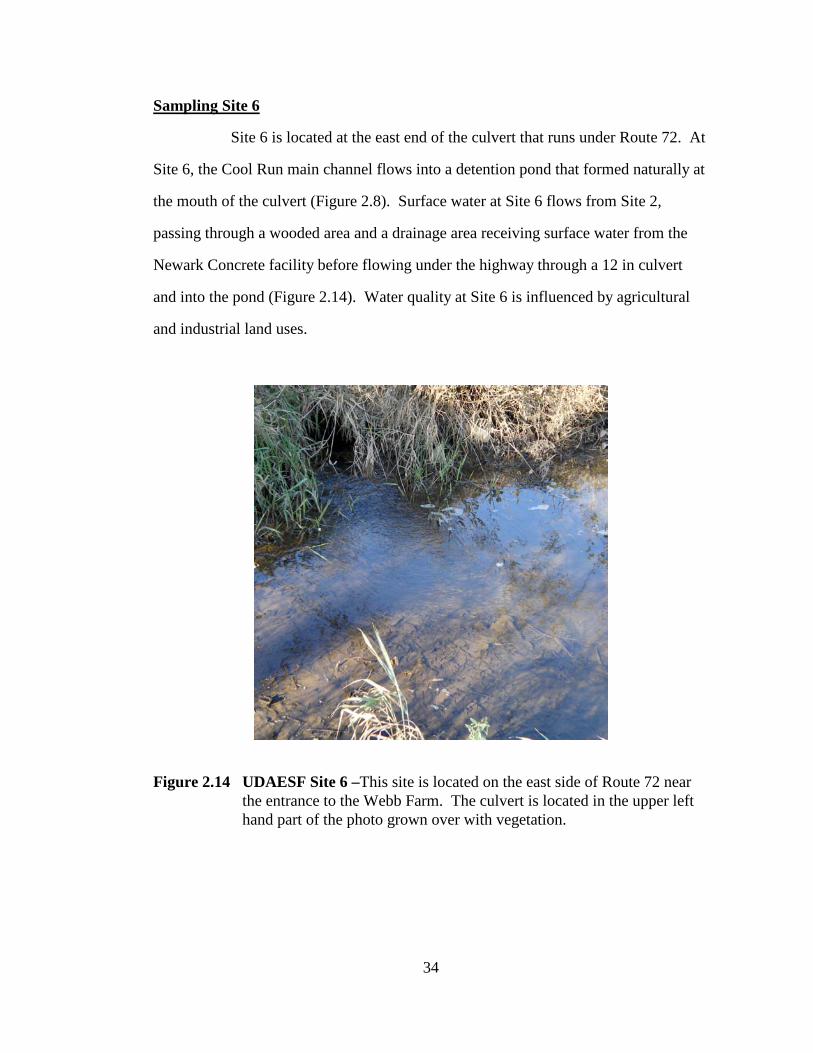
Site 6 is located at the east end of the culvert that runs under Route 72. At

Site 6, the Cool Run main channel flows into a detention pond that formed naturally at

the mouth of the culvert (Figure 2.8). Surface water at Site 6 flows from Site 2,

passing through a wooded area and a drainage area receiving surface water from the

Newark Concrete facility before flowing under the highway through a 12 in culvert

and into the pond (Figure 2.14). Water quality at Site 6 is influenced by agricultural

and industrial land uses.

Figure 2.14 UDAESF Site 6 –This site is located on the east side of Route 72 near the entrance to the Webb Farm. The culvert is located in the upper left hand part of the photo grown over with vegetation.

35

Sampling Site 7

Site 7 is in a stormwater grate located within a constructed wetland

(Figure 2.7). This site was added during the second year of the study in order to

monitor stormwater flows. During storm events, water drains from residential areas

north of the railroad tracks and from the old Newark Delaware Chrysler Assembly

Plant located west of Site 7. The land surrounding the grate was previously used as a

dairy pasture. Due to poor drainage conditions, the pasture was converted to a wetland

and fallow pasture (Figure 2.15). Water quality of the storm samples collected from

the grate is influenced by agricultural, industrial, residential and institutional land uses.

Figure 2.15 UDAESF Site 7 – This site is located near the intersection of Farm Lane and Mopar Drive in the constructed wetland near one of the entrances to the walking path through the wetland.

36

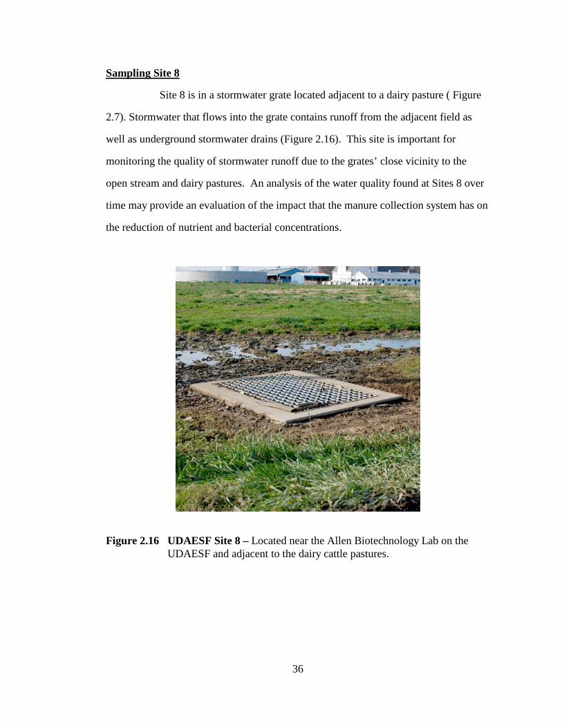
Sampling Site 8

Site 8 is in a stormwater grate located adjacent to a dairy pasture ( Figure

2.7). Stormwater that flows into the grate contains runoff from the adjacent field as

well as underground stormwater drains (Figure 2.16). This site is important for

monitoring the quality of stormwater runoff due to the grates’ close vicinity to the

open stream and dairy pastures. An analysis of the water quality found at Sites 8 over

time may provide an evaluation of the impact that the manure collection system has on

the reduction of nutrient and bacterial concentrations.

Figure 2.16 UDAESF Site 8 – Located near the Allen Biotechnology Lab on the UDAESF and adjacent to the dairy cattle pastures.

37

Characterization of Best Management Practices

Many BMPs have been installed on the NRECF in order to improve the

management of stormwater runoff. These BMPs include constructed wetlands, a

stormwater detention pond, a manure collection system, livestock exclusion fencing,

riparian buffer zones (natural and restored), and a weir to control water movement

from the stormwater detention basin. Figures 2.17 and 2.18 show maps of the NRECF

indicating the locations of the BMPs relative to the monitoring sites and the Cool Run.

Table 2.5 lists the different BMPs installed on the NRECF, their locations, and

installation dates. Information in the table was acquired through personal

communication with the College’s facilities manager, Jenny McDermott.

38

Figure 2.17 BMP Locations on the Newark Research and Education Farm - West side of farm containing sites 1, 3, 4, 7, and 8. (Image: Alison Kiliszek and bing.com)

Figure 2.18 BMP Locations on the Newark Research and Education Farm – East side of farm containing sites 1, 2, 3, 5, and 6. (Image: Alison Kiliszek and bing.com)

39

Table 2.5 BMP Summary. The table summarizes the location and construction times for the different BMPs that are within the UDAESF.

BMP LocationConstruction

Start DateConstruction

End DateConstructed

Wetlands Front Pasture September 8, 2008 October 14, 2008

Gore HallWetlands

Directly Upstream of Gore Hall Weir

OccurredNaturally

OccurredNaturally

Fencing of Stream Within cow pasture land Before 2002 Before 2002

Gore Hall Weir Upstream of Site 2 In 1997 In 1998Manure

Collection Dairy Pasture April 2007 October 2007

Riparian BufferZone Site 7 & Wetland September 8, 2008 October 14, 2008

Riparian BufferZone

Site 8 to Gore Hall Wetland

OccurredNaturally

OccurredNaturally

Riparian BufferZone

Sites 3 & 4to Gore Hall Wetland

OccurredNaturally

OccurredNaturally

Riparian BufferZone

Near Weir, Site 2, ending Site 6

OccurredNaturally

OccurredNaturally

Riparian BufferZone Sites 6 to 5 Occurred

NaturallyOccurredNaturally

Ponding Area Site 6 OccurredNaturally

OccurredNaturally

BMP Summary

Constructed Wetlands

The constructed wetlands are located in the front pasture of the dairy cow

area adjacent to the Girl Scouts of the Chesapeake Bay Headquarters building. Its

design intentions were to replace unproductive and poor performing pastureland with a

more functional ecological system. The area was previously used as a grazing pasture

for the dairy cows until approximately 2005. After years of use by the dairy herd, the

underlying compacted clay layer was formed causing reduced water infiltration with

subsequent ponding and increased stormwater runoff.

The construction of the wetland came in a few different stages. The first

stage of construction included the excavation and installation of a raised outlet pipe

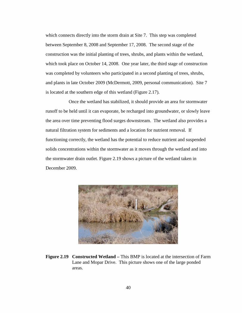
40

which connects directly into the storm drain at Site 7. This step was completed

between September 8, 2008 and September 17, 2008. The second stage of the

construction was the initial planting of trees, shrubs, and plants within the wetland,

which took place on October 14, 2008. One year later, the third stage of construction

was completed by volunteers who participated in a second planting of trees, shrubs,

and plants in late October 2009 (McDermott, 2009, personal communication). Site 7

is located at the southern edge of this wetland (Figure 2.17).

Once the wetland has stabilized, it should provide an area for stormwater

runoff to be held until it can evaporate, be recharged into groundwater, or slowly leave

the area over time preventing flood surges downstream. The wetland also provides a

natural filtration system for sediments and a location for nutrient removal. If

functioning correctly, the wetland has the potential to reduce nutrient and suspended

solids concentrations within the stormwater as it moves through the wetland and into

the stormwater drain outlet. Figure 2.19 shows a picture of the wetland taken in

December 2009.

Figure 2.19 Constructed Wetland – This BMP is located at the intersection of Farm Lane and Mopar Drive. This picture shows one of the large ponded areas.

41

Gore Hall Wetlands Floodplain and Weir

All three tributaries of Cool Run converge and form one 2nd order stream

in an area described as a wetland and/or ponded area (Figure 2.18). Before 1997, this

area was a naturally occurring wetland. In 1997, during the construction of Gore Hall,

located on the headwaters of the Cool Run, the convergence area wetland was

retrofitted and expanded into a stormwater detention basin in order to mitigate the loss

of pervious surface area upstream (Figure 2.20). This area is used for water storage

during storm events to reduce surface runoff and act as a sedimentation basin. A weir

was installed on the downstream side of the basin to prevent flooding and to control

the movement of water through the basin. However, due to poor construction and

maintenance, the weir did not direct the flow of the moving water causing sediment

deposition that filled in the natural stream channel. In 2009, the weir was repaired

allowing the detention basin to function properly and redirecting stream flow through

the natural channel (Figures 2.18 and 2.21). After passing through the weir the Cool

Run flows towards Site 2.

42

Figure 2.20 Gore Hall Wetland – This BMP is located directly upstream of the Gore Hall Weir. The photo was taken looking west standing at the location of the Gore Hall Weir.

Figure 2.21 Gore Hall Weir – This BMP is located at the exit of the Gore Hall Wetland and upstream of Site 2. The photo shows the east (downstream) side of the weir.

43

Livestock Exclusion - Fencing of Streams

Exclusion fencing was installed prior to 2002 by the New Castle County

Conservation District along the Cool Run Stream (Figure 2.18; McDermott, 2009).

One section of fencing runs along the Cool Run between Sites 1 and 2 with sections

adjacent to the Gore Hall Wetland basin and weir. A second section of fence runs

along both sides of the Cool Run between Sites 5 and 6 dividing the pasture into two

sections (Figure 2.18 and 2.22). The fence keeps the animals 2 or more feet away

from the stream edge. One cattle crossing consisting of a concrete pad overlying the

stream is located at Site 5.

Figure 2.22 Fencing of Streams – This BMP shows a portion of the exclusion fencing that is located along the stream throughout of the farm. This photo in particular is of a section downstream of Site 6.

Manure Collection System

Construction of the dairy manure collection system started in April 2007

and was completed in October 2007. The system was operational by December 2007.

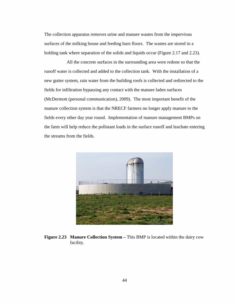
44

The collection apparatus removes urine and manure wastes from the impervious

surfaces of the milking house and feeding barn floors. The wastes are stored in a

holding tank where separation of the solids and liquids occur (Figure 2.17 and 2.23).

All the concrete surfaces in the surrounding area were redone so that the

runoff water is collected and added to the collection tank. With the installation of a

new gutter system, rain water from the building roofs is collected and redirected to the

fields for infiltration bypassing any contact with the manure laden surfaces

(McDermott (personal communication), 2009). The most important benefit of the

manure collection system is that the NRECF farmers no longer apply manure to the

fields every other day year round. Implementation of manure management BMPs on

the farm will help reduce the pollutant loads in the surface runoff and leachate entering

the streams from the fields.

Figure 2.23 Manure Collection System – This BMP is located within the dairy cow facility.

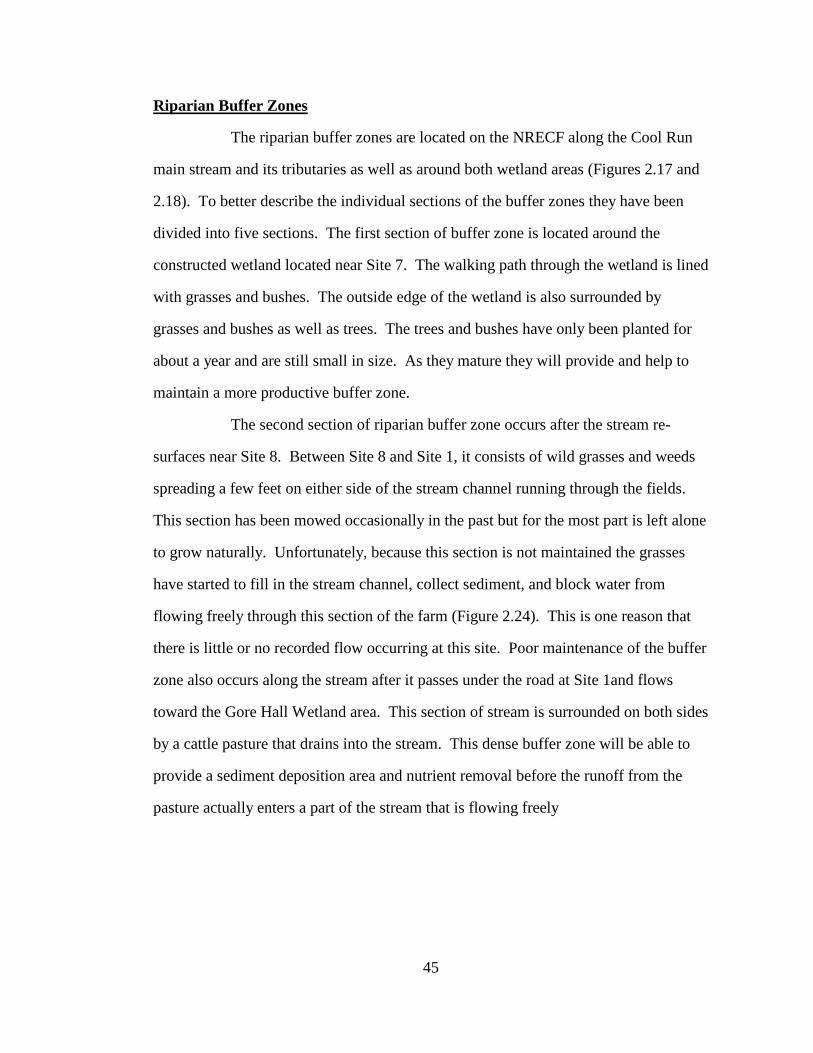
45

Riparian Buffer Zones

The riparian buffer zones are located on the NRECF along the Cool Run

main stream and its tributaries as well as around both wetland areas (Figures 2.17 and

2.18). To better describe the individual sections of the buffer zones they have been

divided into five sections. The first section of buffer zone is located around the

constructed wetland located near Site 7. The walking path through the wetland is lined

with grasses and bushes. The outside edge of the wetland is also surrounded by

grasses and bushes as well as trees. The trees and bushes have only been planted for

about a year and are still small in size. As they mature they will provide and help to

maintain a more productive buffer zone.

The second section of riparian buffer zone occurs after the stream re-

surfaces near Site 8. Between Site 8 and Site 1, it consists of wild grasses and weeds

spreading a few feet on either side of the stream channel running through the fields.

This section has been mowed occasionally in the past but for the most part is left alone

to grow naturally. Unfortunately, because this section is not maintained the grasses

have started to fill in the stream channel, collect sediment, and block water from

flowing freely through this section of the farm (Figure 2.24). This is one reason that

there is little or no recorded flow occurring at this site. Poor maintenance of the buffer

zone also occurs along the stream after it passes under the road at Site 1and flows

toward the Gore Hall Wetland area. This section of stream is surrounded on both sides

by a cattle pasture that drains into the stream. This dense buffer zone will be able to

provide a sediment deposition area and nutrient removal before the runoff from the

pasture actually enters a part of the stream that is flowing freely

46

Figure 2.24 Poorly Maintained Riparian Buffer Zone – This BMP is located throughout the entire site, this was taking looking upstream from Site 1.

The third section of the riparian buffer zone runs along both of the Cool

Run tributaries flowing from north of the farm. The first tributary flows from Site 4 to

the Gore Hall Wetland area while the second tributary flows from Site 3 to the Gore

Hall Wetland area. These are well established, naturally occurring buffers complete

with trees, grasses and dense underbrush in areas. The riparian buffer zone continues

around the edge of the Gore Hall Wetland.

The fourth section of the riparian buffer zone runs along the Cool Run as

it travels from the convergence area through Site 2 and continues to Site 6. There is a

grassy riparian buffer zone with a few scattered trees throughout the section that is

between the Gore Hall Weir and Site 2. After crossing under the access road and the

railroad tracks at Site 2, the Cool Run travels through a densely wooded area, crosses

under Old South Chapel Street through three large culverts and then flows through a

grassy buffer zone before moving through the culvert at Rt. 72.

47

The final section of the riparian buffer zone runs along the Cool Run

within the fenced area as it travels between Site 6 and Site 5.

Figure 2.25 Adequately Maintained Riparian Buffer Zone – This BMP is located throughout the entire site, this was taking looking upstream from Site 5.

Although there is highly dense vegetation lining the banks, the stream flows freely

through the riparian zone (Figure 2.25). There are scattered small trees and bushes

that are mixed in with the grass. The size of the buffer zone varies along this entire

section. From observations after storm events, the fences have been placed outside the

flood zone for normal rain events.

Small Pond

There is a naturally occurring stormwater pond located at Site 6 (Figure

2.18). The pond is fed by two culverts that cross under Route 72. The main stream

flows through a 12 inch diameter culvert while a secondary branch of the Cool Run

and excess storm runoff flow through the larger 5 foot diameter culvert. The pond has

been estimated to be around 3 feet in depth (Figure 2.26). Over the last three years, we

48

have observed the far side of the pond slowly eroding away reducing the size of the

riparian buffer zone surrounding the entire pond.

Figure 2.26 Small Pond – This BMP is located at Site 6, the image was taken looking toward the downstream reach at Site 6.

A history of agronomic management practices was developed and depicted

through a timeline that indicates implementation and construction time of the different

BMPs as well as sample type and sample dates (Figure 2.27). Although the sample

dates are not specially listed on the timeline the two types of samples are indicated by

two different symbols listed in the key.

CARN Cool Run Webb Farm History

SF 7, 8, WetlandSF 7, 8, Wetland

SF 7, 8, Wetland

SF 1-8SF 7 & 8

SF 7 & 8

SF 7 & 8SF 7 & 8

SF 7 & 8SF 7 & 8

SF 7 & 8SF 7 & 8

SF 1-6, 8

SF 7 & 8SF 7 & 8

SF 7 & 8SF 7 & 8

BF 1-6BF 1-6

BF 1 - 6, 8

BF 1-6

BF 1-6

BF 1-6BF 1-6BF 1-6

BF 1-6BF 1-6

BF 1-6

BF 1-6BF 1-6BF 1-6BF 1-6

BF 1-6BF 1-6BF 1-6

BF 1-6BF 1-6BF 1-6BF 1-6BF 1-6BF 1-6

BF 1-6BF 1-6

BF 1-6BF 1-6BF 1-6BF 1-6

BF 1-6

BF 1-6

Aprl 1-6 ?

BF 1-6

BF 1-6

BF 1-6

BF 1-6

BF 1-6

BF 1-6

BF 1-6

Ponding Area (Natural)

Riparian Buffer Zone (Natural)

Manure Collection System

Gore Hall Weir

Fencing Stream Off (Estimated)

Gore Hall Wetland (Stream Junction)

Constructed Wetlands

Jan-97 Sep-97 May-98

Jan-99 Sep-99 Jun-00 Feb-01 Oct-01 Jun-02 Mar-03 Nov-03 Jul-04 Mar-05 Nov-05 Aug-06 Apr-07 Dec-07 Aug-08 Apr-09 Jan-10 Sep-10

Storm Flow (SF) Base Flow (BF) BMPs

BF 1-6

Figure 2.27 CARN Cool Run NRECF History. This is a timeline showing BMP installation and sampling dates.

50

50

Delaware Standards, Delaware Criteria and EPA Water Quality Criteria

In this research work, WQIs were developed using several different

assessment scenarios, which utilized different combinations of the monitored water

quality parameters. In order to develop the subindices for each of these water quality

parameters, concentration values for the regulated standard and/or criteria for each of

the parameters were needed. These values were taken from the State of Delaware

Surface Water Quality Standards (DNREC, 2004). For water quality parameters not

listed by the State of Delaware, standard values were taken from USEPA listings

(USEPA, 2000). As mentioned before, the standard values are set in order to protect

surface water quality in relation to the designated use of the water body under

evaluation. All assessment scenarios were related only to fresh water bodies. A

summary of the general water quality standards for fresh water from the DWQS are

listed in Table 2.6. These criteria relate to any designated use.

51

Table 2.6 General Delaware Fresh Water Quality Standards. These standards are listed in Delaware Surface Water Quality Standards for general fresh water.

PARAMETER WQ STANDARD Temperature No greater than 27.7-30°C

(unless naturally occurring) Dissolved Oxygen Daily Average ≥ 5.5 mg/L

Instantaneous > 4.0 mg/L pH 6.5 – 8.5

Total Suspended Solids

20 mg/L

Turbidity > 10 FTU or NTU Coliforms

(Enterococcus) Single Sample 925/100mL

Geometric Mean 500/100mL {Secondary Contact}

The criteria that will be used for Enterococcus is based on the designated water use of

“secondary contact recreation fresh water.” This contact is defined as a water-based

form of recreation, the practice of which has a low probability for total body

immersion or ingestion of water (examples include but are not limited to wading,

boating and fishing) (DNREC, 2004).

Delaware also has criteria that are specifically related to the protection of

aquatic life in fresh water. Table 2.7 summarizes those values for acute and chronic

exposure limits. Criteria for certain water quality parameters are related to pH or

water hardness of the sample. The values of these related parameters used in the

establishment of the criteria concentrations are given in Table 2.7. A pH of 7.0 and a

Hardness of 100 mg/L CaCO3 were used in calculating the values in Table 2.7 if a

formula required either of the values.

52

The state of Delaware does not specifically state criteria for nitrate in the

protection of aquatic life section, however there is a maximum contaminant level

(MCL) that was specified in the section regarding Human Health Protection. Table

2.8 shows the standard limits of nitrate-nitrogen and fluoride for fish and water

ingestion for systemic toxicants listed in the DWQS document.

Table 2.7 Delaware Water Quality Criteria for Aquatic Life Protection. These criteria are listed in Delaware Surface Water Quality Standards under the section for the protection of aquatic life.

PARAMETER ACUTE (mg/L) CHRONIC (mg/L) Aluminum (pH 6.5 – 9.0)

0.750 0.087

Ammonia (pH 7.0)

24.10 5.97

Arsenic (III) 0.340 0.150 Cadmium

(hardness = 100 mg/L) 0.0025 0.00025

Chromium (III) (hardness = 100mg/L)

0.5698 0.0741

Chromium (VI) 0.016 0.011 Copper

(hardness = 100 mg/L) 0.0134 0.000001

Cyanide 0.022 0.0052 Iron - 1.000 Lead

(hardness = 100 mg/L) 0.06458 0.06391

Mercury 0.0014 0.00077 Nickel

(hardness = 100 mg/L) 0.468 0.052

Selenium 0.020 0.0050 Zinc

(hardness = 100 mg/L) 0.117 0.118

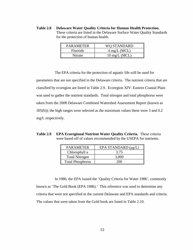
53

Table 2.8 Delaware Water Quality Criteria for Human Health Protection. These criteria are listed in the Delaware Surface Water Quality Standards for the protection of human health.

PARAMETER WQ STANDARD Fluoride 4 mg/L (MCL) Nitrate 10 mg/L (MCL)

The EPA criteria for the protection of aquatic life will be used for

parameters that are not specified in the Delaware criteria. The nutrient criteria that are

classified by ecoregion are listed in Table 2.9. Ecoregion XIV: Eastern Coastal Plain

was used to gather the nutrient standards. Total nitrogen and total phosphorus were

taken from the 2008 Delaware Combined Watershed Assessment Report (known as

305(b)); the high ranges were selected as the maximum values these were 3 and 0.2

mg/L respectively.

Table 2.9 EPA Ecoregional Nutrient Water Quality Criteria. These criteria were based off of values recommended by the USEPA for nutrients.

PARAMETER EPA STANDARD (μg/L) Chlorophyll a 3.75 Total Nitrogen 3,000

Total Phosphorus 200

In 1986, the EPA issued the ‘Quality Criteria for Water 1986’, commonly

known as ‘The Gold Book (EPA 1986).’ This reference was used to determine any

criteria that were not specified in the current Delaware and EPA standards and criteria.

The values that were taken from the Gold book are listed in Table 2.10.

54

Table 2.10 EPA “Gold Book” Criteria. These criteria are based off of values that were from the USEPA Quality Criteria for Water from 1986.

PARAMETER EPA STANDARD (mg/L) Boron* 0.75

Manganese† 0.50 Dissolved Solids 250

*Boron that is naturally occurring in the environment should have no effect on aquatic life. This value is based on long-term irrigation on sensitive crops †Manganese limit for domestic water

No information was found for BOD limits for the Delmarva area. Criteria

for this parameter based on wastewater discharge from The Kansas Department of

Health and Environment Region 7 4B Rationale is shown is Table 2.11 (US EPA,

2008). The values in the table vary by the time of year to help prevent impairment to

the stream from high BOD peaks. The value that will be used in this analysis will set

the upper limit for the BOD concentration at 5 mg/L. This value was chosen fairly low

in comparison to the discharge values (Table 2.11) to try to insure that there would be

a high dilution factor that would prevent impairment.

Table 2.11 EPA Region 7 4B Rationale.

TIME PERIOD EPA CRITERIA September –May 45 mg/L (wkly avg) September – May 30 mg/L (mthly avg)

June – August 40 mg/L (wkly avg) June – August 25 mg/L (mthly avg)

55

Conductivity is not a regulated parameter by Delaware or the EPA,

however, there are optimal ranges described in the USEPA (2006) manual. Water that

has conductivity concentrations out of the ranges listed in Table 2.12 could be

impaired for sustaining certain fish and macro invertebrate species.

Table 2.12 EPA Volunteer Stream Monitoring Manual. The criteria for the conductivity was taken from a Volunteer Stream Monitoring Manual that the USEPA published in 2006.

WATER TYPE EPA STANDARD US Rivers 50 – 1500 μmhos/cm

Inland Fresh Water 150 – 500 μmhos/cm

All the water quality variables that are listed above will be available for

use in the developed model (Objective 2) in order to make the model more diverse and

applicable for many uses. Specific assessments done for this project using the model

may not include all the previously listed quality standards.

Calculation of Subindices

The method in Swamee and Tyagi (2007) states the first step in

developing a WQI is the selection of the parameters that are of most concern. The

next step is to make a set of subindices creating an equal and dimensionless numeric

scale. Finally the subindices are combined to create an overall index value. The

KWQI subindex calculations will use the following equations defined in Swamee and

Tyagi (2000). The WQIs developed for this research were calculated utilizing the 22

parameters that have been monitored in the Cool Run Stream since 2006. In addition,

several different water quality parameters utilized by Swamee and Tyagi (2000, 2007)

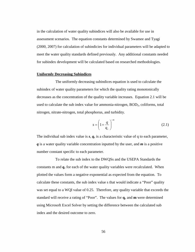
56

in the calculation of water quality subindices will also be available for use in

assessment scenarios. The equation constants determined by Swamee and Tyagi

(2000, 2007) for calculation of subindicies for individual parameters will be adapted to

meet the water quality standards defined previously. Any additional constants needed

for subindex development will be calculated based on researched methodologies.

Uniformly Decreasing Subindices

The uniformly decreasing subindices equation is used to calculate the

subindex of water quality parameters for which the quality rating monotonically

decreases as the concentration of the quality variable increases. Equation 2.1 will be

used to calculate the sub index value for ammonia-nitrogen, BOD5, coliforms, total

nitrogen, nitrate-nitrogen, total phosphorus, and turbidity.

m

cqqs

−

+= 1 (2.1)

The individual sub index value is s, qc is a characteristic value of q to each parameter,

q is a water quality variable concentration inputted by the user, and m is a positive

number constant specific to each parameter.

To relate the sub index to the DWQSs and the USEPA Standards the

constants m and qc for each of the water quality variables were recalculated. When

plotted the values form a negative exponential as expected from the equation. To

calculate these constants, the sub index value s that would indicate a “Poor” quality

was set equal to a WQI value of 0.25. Therefore, any quality variable that exceeds the

standard will receive a rating of “Poor”. The values for qc and m were determined

using Microsoft Excel Solver by setting the difference between the calculated sub

index and the desired outcome to zero.

57

Nonuniformly Decreasing Subindices

The nonuniformly decreasing subindex equation is used on water quality

parameters where the relationship between the rating and the concentration are not

linear. The nonuniformly decreasing subindex accounts for the variability in the rate at

which the quality variables changes with increased concentrations, constants are based

on a threshold concentration. Equation 2.2 will be used to calculate the subindex for

arsenic, chlorophyll a, boron, chromium, cadmium, copper, lead, nickel, and zinc.

Additional water quality parameters that are nonuniformly decreasing include:

aluminum, iron, mercury, selenium, cyanide, and manganese.

44

4

331

1

+

+

+

=

TT

T

qq

qq

qq

s (2.2)

The individual sub index value is s, qT is the threshold concentration for

the specific parameter, and q is the water quality variable concentration inputted by the

user.


constants for each of the quality variables were recalculated. When plotted the values

form a negative S-curve. The constant qT for each of the parameters was calculated

based on conditions to make the threshold limit subindex value 0.25. Therefore, any

quality variable that exceeds the threshold will receive a rating of “Poor”. The value

for qT was determined using Microsoft Excel Solver by setting the difference between

the calculated sub index and the desired outcome to zero.

58

Unimodal Subindices

The unimodal subindices equation is used for parameters that have

optimum values within a water system, the optimum value is considered the point

where s = 1. Equation 2.3 will be used to calculate the subindex for conductivity,

dissolved oxygen, pH, temperature, total dissolved solids and total suspended solids.

The constants for fluoride were calculated for use in the program but were not utilized

in assessments for this project.

pn

T

n

qqrnp

qqrpnpr

s +

−+

−++

=

)1(

)1)((* (2.3)

The individual sub index value is s, p and n are parameter specific constants, q* is the

optimum value for the specific parameter, q is the water quality variable concentration

inputted by the user, and r is the subindex value when q = 0.


constants r, p and n for each of the water quality variables were recalculated. When

plotted the values of s versus concentration form a Bell curve. Constants will be

calculated by a two different methods in this section based on the parameter. The first

method is to use the sum of the difference of the desired and calculated WQI subindex

value. This method is used for parameters that have optimum ranges such as pH and

conductivity. The other method is to run a series of trials until the concentration

values fit the desired WQI concentration plot.

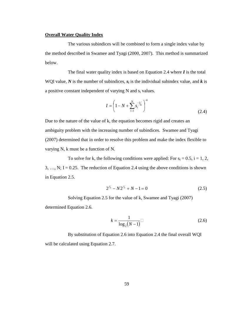
59

Overall Water Quality Index

The various subindices will be combined to form a single index value by

the method described in Swamee and Tyagi (2000, 2007). This method is summarized

below.

The final water quality index is based on Equation 2.4 where I is the total

WQI value, N is the number of subindices, si is the individual subindex value, and k is

a positive constant independent of varying N and si values.

kN

i

kisNI

−

=

−

+−= ∑

1

11

(2.4)

Due to the nature of the value of k, the equation becomes rigid and creates an

ambiguity problem with the increasing number of subindices. Swamee and Tyagi

(2007) determined that in order to resolve this problem and make the index flexible to

varying N, k must be a function of N.

To solve for k, the following conditions were applied: For si = 0.5, i = 1, 2,

3, …, N; I = 0.25. The reduction of Equation 2.4 using the above conditions is shown

in Equation 2.5.

0122 12=−+− NN kk (2.5)

Solving Equation 2.5 for the value of k, Swamee and Tyagi (2007)

determined Equation 2.6.

( )1log1

2 −=

Nk � (2.6)

By substitution of Equation 2.6 into Equation 2.4 the final overall WQI

will be calculated using Equation 2.7.

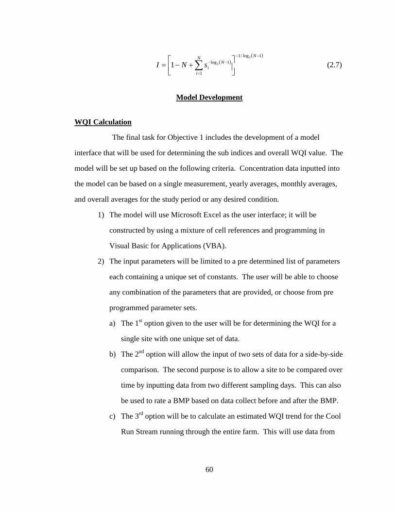
60

( )( )1log/1

1

1log2

21−−

=

−−

+−= ∑

NN

i

NisNI (2.7)

Model Development

WQI Calculation

The final task for Objective 1 includes the development of a model

interface that will be used for determining the sub indices and overall WQI value. The

model will be set up based on the following criteria. Concentration data inputted into

the model can be based on a single measurement, yearly averages, monthly averages,

and overall averages for the study period or any desired condition.

1) The model will use Microsoft Excel as the user interface; it will be

constructed by using a mixture of cell references and programming in

Visual Basic for Applications (VBA).

2) The input parameters will be limited to a pre determined list of parameters

each containing a unique set of constants. The user will be able to choose

any combination of the parameters that are provided, or choose from pre

programmed parameter sets.

a) The 1st option given to the user will be for determining the WQI for a

single site with one unique set of data.

b) The 2nd option will allow the input of two sets of data for a side-by-side

comparison. The second purpose is to allow a site to be compared over

time by inputting data from two different sampling days. This can also

be used to rate a BMP based on data collect before and after the BMP.

c) The 3rd option will be to calculate an estimated WQI trend for the Cool

Run Stream running through the entire farm. This will use data from

61

any combination of Sites 1 to 8. Limitations include the assumption

that between sampling points there is an equal gradient between the

WQI values. To use this plot a flow value must be entered for Sites 1,

3 and 4 on the input screen if values are desired for Site 2.

3) The outputted data will include the following:

a) For the 1st and 2nd options:

i) A list of each parameter that shows the individual WQI sub index

value and the rating associated with that value.

ii) A plot of each parameter’s sub index value with the value indicated

on the plot.

iii) An overall WQI value and the rating associated with it.

iv) A table summarizing the number of parameters that received each

rating.

v) A plot of the distribution of received ratings.

b) For the 2nd option only:

i) The percent change between the two values will be calculated.

ii) The percent change for each subindex will also be plotted.

c) For 3rd option only

i) For each site slot used for data the overall WQI value will be given

and the rating that is associated to that value.

ii) A spatial 3D plot of the farm will be constructed based on the

calculated WQI values. The plot is based on inputting the

calculated WQI values into the site locations and then interpolating

the parts of the stream between sites. For simplification of

62

calculations this assumes an even distribution based on the

estimated pixel parcels between sites. The values are only meant to

simulate the values in the stream and to show basic trends that

occur within the NRECF.

Model Validation

The first tests will use Cool Run water quality monitoring data collected

and reported in Harrell (2001). The data will be used as a basis for water quality

before the installation of BMPs in the watershed. Five of the sites that were used in

Harrell (2002) are close to or the same as the ones that have been used in this study.

The data will also be used to test and calibrate the parameters to be used in the final

model.

The second part of the test will include selecting multiple parameter sets

based on common indicators used to determine water quality based on water use

requirements. As previously stated, the water uses requirements will be based on

quality variables determined by DNREC and the USEPA. From this, tests will be run

to show the effect of different parameters on the overall WQI. This will also be used

in the attempt to determine a minimum, optimum and maximum number of parameters

that should be used.

Assessment of BMP Efficiency

The final objective of determining the effects of the BMPs will be

achieved by using the model to make comparisons. Comparisons will include point to

point comparisons over time, trends at individual sites, and an estimation of trends for

63

the farm over time as well as changes in water quality after installation of the BMPs.

The following steps will be taken to accomplish the assessments.

1) Since data from Sites 2, 3, and 4 are available for a base line of water quality

before the BMPs were implemented, the WQI values will be used to make

point to point comparisons between 2001 and the data collected in 2009.

2) Site 2 is fed from Sites 1, 3, and 4, speculations and comparisons will be made

to relate what happens to water quality as the Cool Run flows through the farm

to Site 2.

3) Sites 2 and 6 are located closest together. A comparison of the WQI values and

trends between these sites in relationship to land use could show how land use

influences water quality over short distances.

4) The comparison between Sites 5 and 6 will assess the effect of riparian buffer

zones and exclusion fencing on water quality.

5) Site 8 primarily measures the quality of stormwater runoff from a nearby

pasture area. The water quality data from this site can be evaluated over time

to show how the runoff water quality has changed over time during storm

events after the installation of the manure collection system.

6) An overall comparison of water quality at all monitoring sites will be made

based on the calculated WQIs. The same parameter sets will be used to

evaluate each of the sites on the same level for each of the years to determine

trends in the WQI ratings.

7) The final analysis will be done using parameter sets that relate to the removal

capabilities of the individual BMPs installed near the different monitoring

sites. Once the parameter set is chosen, it will be used for that site in all the

64

analysis. This will be done to provide an assessment of the efficiency of the

BMPs on water quality improvement and to draw conclusions of how the sites

have been affected over the years.

65

Chapter 3

RESULTS AND DISCUSSION

Annual water quality data from the Cool Run monitoring program

indicates that several of the Cool Run tributaries have elevated levels of nutrients,

bacteria and suspended solids (Tables 3.1, 3.2 and 3.3). In general, metal

concentrations were below Delaware’s water quality criteria. However, copper

concentrations exceeded the criteria limits. The highest concentrations of copper were

found at Site 3 where the tributary flows through an old industrial area. Water quality

values for Site 1 showed the greatest impairment with the highest ammonia nitrogen

(0.92- 2.10 mg l-1) and total phosphorus concentrations (1.46-2.02 mg l-1) and the

lowest flow volumes.

The annual water quality data was used in the calculation of the Kiliszek

WQI (KWQI). Subsequently, the calculated KWQIs were used to evaluate the general

health of the Cool Run and its tributaries located on the NRECF. The KWQIs were

also used in the model comparisons of water quality at the monitoring sites and in the

assessments and evaluations of the installed BMPs.

Table 3.1 Average Annual Concentrations of Monitored Water Quality Parameters- 2006

2006 Parameter 1 2 3 4 5 6 7 8

Ammonia-N (NH4-N) (mg/L) 2.10 0.39 0.11 0.06 0.16 0.24 Nitrates (NO3-N) (mg/L) 0.93 3.22 4.29 3.25 3.15 2.91

Total Nitrogen (mg/L) 5.20 4.12 4.62 3.66 3.82 3.86 Total Phosphorus (mg/L) 2.02 0.22 0.51 0.06 0.16 0.20

Arsenic(III) (mg/L) 0.0222 0.0085 0.0015 0.0110 0.0045 0.0110 Boron (mg/L) 0.0535 0.0393 0.0295 0.0875 0.0370 0.0450

Cadmium (mg/L) 0.0008 0.0008 0.0001 0.0008 0.0005 0.0005 Chromium (III) (mg/L) 0.0012 0.0013 0.0010 0.0000 0.0000 0.0000

Copper (mg/L) 0.0111 0.0240 0.0368 0.0131 0.0207 0.0198 Lead (mg/L) 0.0049 0.0103 0.0086 0.0148 0.0103 0.0135

Nickel (mg/L) 0.0270 0.0225 0.0240 0.0220 0.0240 0.0240 Zinc (mg/L) 0.0309 0.0499 0.0699 0.0564 0.0458 0.0716

BOD5 (mg/L) 5.04 2.40 2.40 2.40 2.40 2.40 DO (mg/L) 3.11 7.23 8.87 6.82 9.10 7.96

Temperature (°C) 16.66 18.32 19.39 18.23 19.25 18.43 pH 6.80 6.74 6.93 6.64 6.99 6.93

Conductivity (mS/cm) 0.431 0.910 1.370 1.650 0.952 1.774 Turbidity (mg/L) 11.25 13.50 9.00 3.00 12.25 9.75

Chlorophyll a (mg/L) 0.0120 0.0051 0.0010 0.0037 0.0054 0.0072 Coliform bacteria (1 sample) 10439 10077 10450 4144 9772 1908

Total Dissolved Soilds (mg/L) 113 160 183 188 171 176 Total Suspended Solids (mg/L) 33 15 6 13 9 20

Flow (m3/s) 0.0069 0.2383 0.0312 0.0287 0.0628 0.1668

67


2007 Parameter 1 2 3 4 5 6 7 8

Ammonia-N (NH4-N) (mg/L) 1.79 0.57 0.24 0.23 0.40 0.72 0.53 3.70 Nitrates (NO3-N) (mg/L) 3.55 3.81 3.81 3.47 3.69 3.59 1.06 1.41

Total Nitrogen (mg/L) 7.06 5.29 4.56 4.10 4.67 4.69 3.27 4.43 Total Phosphorus (mg/L) 1.46 0.18 0.27 0.07 0.18 0.17 0.30 2.83

Arsenic(III) (mg/L) 0.0093 0.0158 0.0108 0.0078 0.0073 0.0090 0.0077 0.0087 Boron (mg/L) 0.0463 0.0713 0.0563 0.1010 0.0713 0.0585 0.0302 0.0484

Cadmium (mg/L) 0.0015 0.0018 0.0021 0.0014 0.0015 0.0015 0.0057 0.0007 Chromium (III) (mg/L) 0.0123 0.0083 0.0058 0.0048 0.0043 0.0143 0.0145 0.0082

Copper (mg/L) 0.0142 0.0389 0.4015 0.0173 0.0246 0.0521 0.0330 0.0193 Lead (mg/L) 0.0083 0.0131 0.0081 0.0052 0.0052 0.0227 0.0087 0.0059

Nickel (mg/L) 0.0350 0.0574 0.1035 0.0483 0.0468 0.1933 0.0288 0.0138 Zinc (mg/L) 0.0587 0.0698 0.0961 0.0527 0.0468 0.1202 0.3807 0.1383

BOD5 (mg/L) 2.40 4.98 3.59 5.23 3.62 3.47 0.00 0.00 DO (mg/L) 3.00 6.99 8.26 6.86 8.18 8.41 4.82 2.51

Temperature (°C) 12.09 14.70 16.98 14.55 14.36 14.12 18.62 19.42 pH 6.30 6.44 6.80 6.60 6.71 6.65 5.76 6.62

Conductivity (mS/cm) 0.506 0.705 1.325 0.754 0.722 0.752 0.677 1.008 Turbidity (mg/L) 29.63 20.25 10.25 3.88 7.63 17.13 0.00 0.00

Chlorophyll a (mg/L) 0.0421 0.0089 0.0027 0.0026 0.0058 0.0101 0.0048 0.0049 Coliform bacteria (1 sample) 1872 5438 1510 7938 4201 3899 54767 1191660

Total Dissolved Soilds (mg/L) 396 559 1000 585 550 577 499 721 Total Suspended Solids (mg/L) 64 30 6 6 29 22 113 49

Flow (m3/s) 0.0001 0.2279 0.0648 0.0047 0.0437 0.2790 0.0000 0.0000

68


2008 Parameter 1 2 3 4 5 6 7 8







BOD5 (mg/L) 4.57 2.40 2.40 2.40 2.40 2.40 0.00 0.00 DO (mg/L) 1.58 4.48 5.59 5.05 6.05 6.23 4.78 4.60

Temperature (°C) 11.23 12.20 13.94 12.94 12.21 12.19 10.86 13.54 pH 6.13 6.39 6.61 6.50 6.74 6.63 6.20 6.49


Chlorophyll a (mg/L) 0.0274 0.0052 0.0024 0.0055 0.0056 0.0131 0.0069 0.0126 Coliform bacteria (1 sample) 2075 1439 853 1259 1318 1749 13846 596740


Flow (m3/s) 0.0001 0.1508 0.0228 0.0168 0.0432 0.2185 0.0000 0.0000

69


2009 Parameter 1 2 3 4 5 6 7 8







BOD5 (mg/L) 4.67 2.76 2.53 2.40 2.81 2.40 0.00 0.00 DO (mg/L) 2.14 6.94 8.65 7.45 8.80 8.36 3.80 3.22

Temperature (°C) 13.89 16.09 16.17 15.83 14.46 13.97 10.65 10.38 pH 6.73 6.83 7.04 6.86 6.90 6.96 6.60 6.24


Chlorophyll a (mg/L) 0.0154 0.0095 0.0070 0.0024 0.0073 0.0146 0.0227 0.0086 Coliforms (1 sample) 8066 819 838 1503 1023 1245 3000 3600


Flow (m3/s) 0.0001 0.1464 0.0276 0.0126 0.0585 0.1816 0.0000 0.0000

70

70

The methodology used in the work for the KWQI development was based

on a modification of the National Sanitation Foundation’s Water Quality Index

[NSFWQI] (Syamee and Tyagi, 2000, 2007). The NSFWQI used curves to relate

concentration of various water quality parameters to subindices. The subindices were

then aggregated into a single water quality index. The subindices equations were

developed using a consensus of national criteria, state standards and information

developed from the literature (Swamee and Tyagi, 2000). For this work, the three

generic subindex equations developed by Swamee and Tyagi were modified using the

State of Delaware water quality standards. For water quality parameters not addressed

in the State of Delaware’s regulations, standard values were based on USEPA eco-

region XIV criteria. This modification resulted in the alteration of the equation

constants as outlined below.

Determination of Subindex Equation Constants

The modifications that were made to the subindex equations constants

were made using Microsoft Excel Solver. The solver function was set to make the

difference between the desired sub-WQI value and the calculated sub-WQI to be zero.

The desired sub-WQI value associated with the calculated sub-WQI was different for

each water quality parameter and was based on the standards or criteria that were set

by the state for the designated water use. Before adapting the constants to meet the

standards and criteria for the Cool Run watershed, the unmodified equations from

Swamee and Tayagi (2000 & 2007) were run through the solver function using water

quality values used in their research. Agreement between the constant values derived

through the solver to those provided by Swamee and Tyagi (2000) verified the

accuracy of the modification method. After verification was achieved for the 3

71

subindice equations, the solver was used to determine the modified constants required

for every water quality parameter as described below.

The uniformly decreasing subindex was determined by setting the desired

sub-WQI value to 0.25. In this subindex, parameters with concentrations greater than

the allowable limit received a rating of poor. An initial number similar to the value of

the provided sub-WQI constant was used as a starting point for the solver.

The nonuniformly decreasing subindex constants are determined based on

the threshold concentration of each parameter. Similar to the uniformly decreasing

subindex values, the desired calculated sub-WQI value was set to 0.25. Any value that

is greater than the threshold limit would receive a rating of poor. The initial number

that was used in the solver function was the threshold concentration of the parameter

or a value very similar to it.

The unimodal subindices constants were determined using two different

methods of calculation. Both methods were dependant on the individual parameter

and the acceptable range for the parameter. When solving for the constants for pH,

temperature, and TSS the desired sub-WQI values were set to be 0.51. Initially all the

parameter constants were calculated based on a sub-WQI value of 0.25. When these

parameters were being tested in the initial stages of model development, the sub-WQI

vs. Concentration curves (discussed in following sections) did not make sense. The

natural average pH value from the monitoring data was on the lower boundary of the

acceptable pH range listed in the Delaware standards. Many of the documents

reporting standards and criteria for water quality parameters state that there are

optimum levels for some parameters but that naturally occurring concentrations may

not fall within the provided range. The criteria values for temperature and TSS

72

behaved similarly to those for pH. These curves were also adjusted to fit naturally

occurring regional values. The sub-WQI for conductivity, TDS and fluoride were all

calculated based on the criteria limits set equal to a sub-WQI value of 0.25.

Many of the parameters have acute and chronic exposure limits described

in the water quality criteria by Delaware and the USEPA. To make the KWQI

program more diverse, the sub-WQI constants for acute and chronic limits were

calculated and will be able to be used in the KWQI program.

Comparison of Determined Constants

The modified and unmodified values for qT used in the nonuniformal

subindex equation are listed in Table 3.5. The water quality parameters that were used

in the Swamee and Tyagi (2000 & 2007) sub-index equations had only a single criteria

value for calculations. The KWQI divided the exposure limits into acute and chronic

values to make the model useful for estimating long term effects on the stream water

quality. There is much variability between the modified and unmodified constant

values. This variability can be attributed to the difference in state regulations and

criteria values. Some states break down every water quality parameter into individual

water uses while others may only separate them into fresh or marine water categories.

It was not stated what water use or if the limits were for chronic or acute exposure in

the criteria values used by Swamee and Tyagi (2000 & 2007). Also, regulation

standards and criteria values vary spatially and temporally. Constant values calculated

for water quality parameters not addressed by Swamee and Tyagi are also included in

Table 3.5.

73

Table 3.5 Nonuniformal Subindex qT Constants – Includes values from Swamee and Tyagi (2000 & 2007) and calculated constants

Parameter Unit S&T* Acute ChronicAluminum mg/L 0.20 0.72 0.08Arsenic mg/L 0.05 0.33 0.14Boron mg/L - - 0.72Cadmium mg/L 0.0005 0.0024 0.0002Chlorophyll a mg/L - 0.0036 -Chromium mg/L 0.050 - -Chromium (III) mg/L - 0.547 0.071Chromium (VI) mg/L - 0.015 0.011Copper mg/L 0.050 0.013 0.009Cyanide mg/L 0.050 0.024 0.005Iron mg/L 0.10 0.96 -Lead mg/L 0.05 0.06 0.06Manganese mg/L 0.05 - 0.05Mercury mg/L 0.001 0.001 0.001Nickel mg/L - 0.449 0.050Selenium mg/L 0.010 0.019 0.005Zinc mg/L 5.000 0.112 0.113* S&T are values from Swamee and Taygi (2000 & 2007)

Nonuniformal Subindex qT Constants

The modified and unmodified values of the different constants used in the

uniform subindex equation are listed in Table 3.6. The constants were calculated for

five water quality parameters: BOD5, coliform bacteria, nitrogen, phosphorus and

turbidity. The BOD5 constants taken from Swamee and Tyagi (2000 & 2007) did not

state whether they were for a monthly or weekly average. The criteria values used to

calculate the modified equation constants were divided into acceptable values for the

time of year and for weekly or monthly averages. The modified and unmodified

constants for BOD5 are similar with little variation among the separate criteria values.

74

Table 3.6 Uniform Subindex Constants - Includes values from Swamee and Tyagi (2000 & 2007) and calculated constants

Parameter Unit m qcBOD5* mg/L 3.0 20.0BOD5 mg/L 1.2 20.1

Coliforms* MPN/100mL 0.30 4.00Coliforms (geometric mean) MPN/100mL 0.29 4.00Coliforms (single sample) MPN/100mL 0.27 5.00

Nitrates (NO3-N)* mg/L 3.0 40.0Nitrate (NO3-N) mg/L 6.2 39.8Total N mg/L 6.2 19.9Ammonia (NH4-N) (acute) mg/L 6.4 99.0Ammonia (NH4-N) (chronic) mg/L 23.1 96.9

Phosphates* mg/L 1.0 0.67Total P mg/L 612.3 88.2

Turbidity* JTU 1.5 50.0Turbidity JTU 6.2 39.8*Values are from Swamee and Taygi (2000 & 2007)

Uniform Subindex Constants

The modified and unmodified values for sub-index constants for coliform bacteria

were similar, which indicates similar criteria standards were used in the calculations.

Swamee and Tyagi (2000 & 2007) only calculated the values for the sub-index

constants for nitrate. Sub-index constant values were calculated for ammonia nitrogen

and total nitrogen in order to include these water quality parameters in the assessment

model. Values for sub-index constants for acute and chronic exposure limits were

calculated for ammonia nitrogen. There were no criteria for phosphate regulation in

the Delaware standards so a comparison between modified and unmodified values

could not be made. However, the criteria for total phosphorus, found within USEPA

documents, were used to calculate the values of the sub-index constants. The

75

modified and unmodified values for the turbidity sub-index constants were quite

different indicating large differences between the states’ regulations and criteria.

The values of the modified and unmodified constants that are to be used

with the unimodal subindex equation are listed in Table 3.7. Conductivity was the

only parameter that was not utilized by Swamee and Tyagi (2000 & 2007), so no

comparison could be made between values. Comparison between the modified and

unmodified values of the sub-index constant for DO was difficult to make because of

the difference in criteria units (units of proportion vs. mg l-1). The modified and

unmodified values of the sub-index DO constant s for q* are very different, however,

the values for the sub-index constants n, p, and r are similar. Although fluoride is not

used in this project the values for the sub-index constants for the parameter were

determined for use in the KWQI if desired. The modified and unmodified values of

the sub-index pH constants were identical for q* but fairly different for the other

constants. This was the direct result of not using just the optimum criteria value for

pH. Instead, the solver set the range of optimum values so that anything out of range

would receive a rating of fair or lower. Swamee and Tyagi (2000 & 2007) used the

total of the suspended and dissolved solids for calculations of the sub-index constants.

However, the state of Delaware has water quality criteria set for each individual

parameter. For this reason the, TDS and the TSS were utilized as separate parameters

in the KWQI. Therefore, no comparisons could be made. The modified and

unmodified values of the sub-index constant for temperature were expected to be

different because of the variance in optimum temperatures for different ecoregions.

76

Table 3.7 Unimodal Subindex Constants - Includes values from Swamee and Tyagi (2000 & 2007) and calculated constants

Parameter Unit q* n p rConductivity mS/cm 0.36 0.89 1.79 0.02

Dissolved Oxygen* proportion 1.0 3.0 1.0 0.0DO (daily average) mg/L 9.6 4.2 2.4 0.0DO (instantaneous) mg/L 8.3 3.4 1.6 0.0

Fluoride* mg/L 1.0 4.0 4.0 0.0Fluoride mg/L 2.4 4.0 4.0 0.0

pH* - 7.0 4.0 6.0 0.0pH - 7.3 9.1 10.2 0.0

Total Solids (TDS+TSS)* mg/L 75.0 1.0 1.0 0.8TDS mg/L 5.0 1.0 1.1 0.8TSS mg/L 30.0 0.9 1.1 0.8

Temperature* °C 20.0 0.5 7.0 0.0Temperature °C 20.1 1.8 4.8 0.4* Values are from Swamee and Taygi (2000 & 2007)

Unimodal Subindex Constants

Comparison of the Sub-KWQI to Water Quality Parameter Concentration

The sub-KWQI values were plotted against the water quality parameter

concentrations in order to demonstrate the relationship among the sub-KWQI, the

associated concentration and the rating scores. The plots include four additional

horizontal lines that mark the division of the five different ratings (Poor, Fair,

Average, Good and Excellent) that a water quality parameter sub-index can represent.

Any calculated index values that are below the red line will receive a rating of “Poor”.

Values that fall between the red and orange lines will have a rating of “Fair”. Values

that occur between the orange and yellow lines receive a rating of “Average”. A rating

of “Good” is received when the calculated value is located between the yellow and

green line. Any value that is above the green line will receive an “Excellent” rating.

77

The uniform subindex equation creates an exponentially decreasing plot

where the sub-index increases with decreasing concentration. The relationship

between concentration and sub-indices for ammonia nitrogen is shown in Figure 3.1.

The difference in the concentration values that exceeds the state criteria between the

acute and chronic exposure for ammonia nitrogen increases significantly as the rating

decreases from excellent to poor. The difference between the acute concentration and

chronic concentration for an excellent rating is approximately 1.6 mg l-1 while the

difference for a poor rating is 18.00 mg l-1. Therefore, the sub-KWQI will vary greatly

and be dependent on the type of exposure under evaluation. The sub-indice values for

the acute exposure limit are used for calculations in the model assessments because we

were evaluating changes in water quality over short periods of time.

Ammonia

Acute Exposure

Chronic Exposure

0.00.10.20.30.40.50.60.70.80.91.0

0 2 4 6 8 10 12 14 16 18 20 22 24 26 28 30

mg/L

sub-

WQ

I Val

ue

Figure 3.1 Uniform Sub-KWQI Versus Concentration Curve - Ammonia

78

Unlike the ammonia sub-indices, the relationship between concentration and the sub-

KWQI for BOD5 is similar regardless of whether monthly or weekly averages are used

(Figure 3.2). Criteria concentrations for weekly averages are allowed to be higher

assuming that averages for the month are within the tolerable ranges. The differences

in the concentration values that exceeds the state criteria between the weekly average

and the monthly average for BOD5 are similar for both the September to May and the

June to August time periods. The difference between the weekly average and the

monthly average values for an average rating is approximately 5 mg l-1 while the

difference for a poor rating is 16.00 mg l-1 for both time periods. When using the sub-

KWQI in model assessments for yearly averages, it is best to use the September to

May values.

The relationship between the sub-KWQI and coliform concentration is

shown in Figure 3.3. This concentration criteria used to create the curves assumes that

at times a single sample measurement may be higher than expected but that an average

of several measurements will fall below the occasional peak values. Therefore, the

concentrations receiving poor ratings are 925 and 500 CFU per 100 ml for single

sample and geometric mean sample, respectively, whereas the concentrations receiving

average ratings are 80 and 50 CFU per 100 ml, respectively.

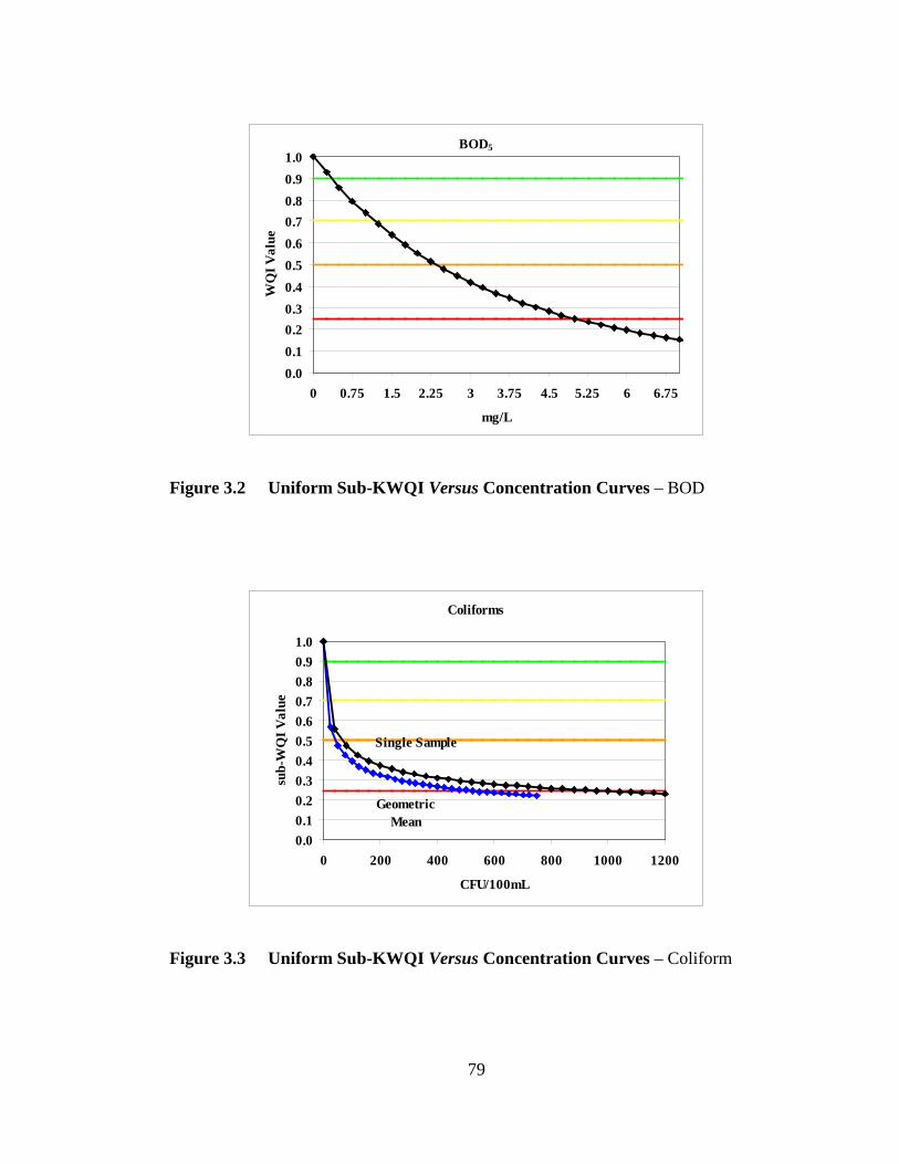
79

BOD5

0.00.10.20.30.40.50.60.70.80.91.0

0 0.75 1.5 2.25 3 3.75 4.5 5.25 6 6.75

mg/L

WQ

I Val

ue

Figure 3.2 Uniform Sub-KWQI Versus Concentration Curves – BOD

Coliforms

Geometric Mean

Single Sample

0.00.10.20.30.40.50.60.70.80.91.0

0 200 400 600 800 1000 1200

CFU/100mL

sub-

WQ

I Val

ue

Figure 3.3 Uniform Sub-KWQI Versus Concentration Curves – Coliform

80

The regulations and criteria for turbidity, nitrate, total nitrogen and total

phosphorus only state that there is a maximum value that should not be exceeded.

Concentration measurements that were greater than the criteria would result in a poor

rating for water quality. Figures 3.4 and 3.5 illustrate the relationship between the

sub-KWQI value and the parameter concentration for turbidity and nitrate-nitrogen. A

water body receiving a rating of excellent will have concentrations equal to or less

than 0.5 JTU and 0.8 mg l-1 for turbidity and nitrate nitrogen, respectively. Figures 3.6

and 3.7 illustrate the relationship between the sub-KWQI value and the parameter

concentration for total nitrogen (TN) and total phosphorus (TP). A water body

receiving a rating of excellent will have concentrations equal to or less than 1.25 and

0.0036 mg l-1 for TN and TP, respectively. The rating falls below average when

concentrations reach 15.0 and 0.027 mg l-1 for TN and TP, respectively.

Turbidity

0.00.10.20.30.40.50.60.70.80.91.0

0 1 2 3 4 5 6 7 8 9 10 11 12 13 14 15

JTU

sub-

WQ

I Val

ue

Figure 3.4 Uniform Sub-KWQI Versus Concentration Curves - Turbidity

81

Nitrate

0.00.10.20.30.40.50.60.70.80.91.0

0 1 2 3 4 5 6 7 8 9 10 11 12

mg/L

sub-

WQ

I Val

ue

Figure 3.5 Uniform Sub-KWQI Versus Concentration Curves – Nitrate

Total Nitrogen

0.00.10.20.30.40.50.60.70.80.91.0

0 0.5 1 1.5 2 2.5 3 3.5

mg/L

sub-

WQ

I Val

ue

Figure 3.6 Uniform Sub-KWQI Versus Concentration Curves – Total Nitrogen

82

Total Phosphorus

0.00.10.20.30.40.50.60.70.80.91.0

0 0.04 0.08 0.12 0.16 0.2 0.24

mg/L

sub-

WQ

I Val

ue

Figure 3.7 Uniform Sub-KWQI Versus Concentration Curves – Total Phosphorus

The relationship between the nonuniformal subindex values and

concentration for aluminum and cadmium behaves quite differently for the acute and

chronic exposures (Figures 3.8 and 3.9). The steeper slope of the chronic exposure

curve indicates a greater change in the sub-KWQI value for smaller changes in

concentration. For ratings ranging between excellent and poor, the concentrations

range from 0.039 to 0.087 and from 0.338 to 0.754 mg l-1 for chronic and acute

aluminum exposures, respectively. Similarly, for ratings ranging between excellent

and poor, the concentrations range from 0.00011 to 0.00024 and from 0.0011 to

0.0025 mg l-1 for chronic and acute cadmium exposures, respectively. The rating

concentrations for acute exposure measurements are 10 times higher than the rating

concentrations for chronic exposure measurement. The relationship between the

nonuniformal subindex value and concentration for chromium (III) and cyanide are

83

shown in Figures 3.10 and 3.11. The relationship behaves quite differently for the

acute and chronic exposures. For ratings ranging between excellent and poor, the

concentrations range from 0.035 to 0.0725 and from 0.260 to 0.560 mg l-1 for chronic

and acute chromium (III) exposures, respectively. Similarly, for ratings ranging

between excellent and poor, the concentrations range from 0.0024 to 0.0052 and from

0.011 to 0.025 mg l-1 for chronic and acute cyanide exposures, respectively. The

relationship between the nonuniformal subindex value and concentration for nickel

and selenium are shown in Figures 3.12 and 3.13. As for the other parameters

discussed above, the relationship behaves quite differently for the acute and chronic

exposures. For ratings ranging between excellent and poor, the concentrations range

from 0.024 to 0.052 and from 0.220 to 0.460 mg l-1 for chronic and acute nickel

exposures, respectively. Similarly, for ratings ranging between excellent and poor, the

concentrations range from 0.0022 to 0.0050 and from 0.009 to 0.0203 mg l-1 for

chronic and acute selenium exposures, respectively. Both the acute and chronic

exposure parameters will be able to be utilized in the KWQI model to calculate the

overall KWQI.

84

Aluminum

Acute Exposure

Chronic Exposure

0.00.10.20.30.40.50.60.70.80.91.0

0 0.2 0.4 0.6

mg/L

sub-

WQ

I Val

ue

Figure 3.8 Nonuniform Sub-KWQI Versus Concentration Curves – Aluminum

Cadmium

Acute Exposure

Chronic Exposure

0.00.10.20.30.40.50.60.70.80.91.0

0.0000 0.0005 0.0010 0.0015 0.0020 0.0025 0.0030

mg/L

sub-

WQ

I Val

ue

Figure 3.9 Nonuniform Sub-KWQI Versus Concentration Curves – Cadmium

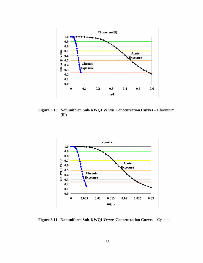
85

Chromium (III)

Acute Exposure

Chronic Exposure

0.00.10.20.30.40.50.60.70.80.91.0

0 0.1 0.2 0.3 0.4 0.5 0.6

mg/L

sub-

WQ

I Val

ue

Figure 3.10 Nonuniform Sub-KWQI Versus Concentration Curves – Chromium (III)

Cyanide

Acute Exposure

Chronic Exposure

0.00.10.20.30.40.50.60.70.80.91.0

0 0.005 0.01 0.015 0.02 0.025 0.03

mg/L

sub-

WQ

I Val

ue

Figure 3.11 Nonuniform Sub-KWQI Versus Concentration Curves – Cyanide

86

Nickel

Acute Exposure

Chronic Exposure

0.00.10.20.30.40.50.60.70.80.91.0

0.000 0.100 0.200 0.300 0.400 0.500 0.600

mg/L

sub-

WQ

I Val

ue

Figure 3.12 Nonuniform Sub-KWQI Versus Concentration Curves – Nickel

Selunium

Acute Exposure

Chronic Exposure

0.00.10.20.30.40.50.60.70.80.91.0

0 0.005 0.01 0.015 0.02

mg/L

sub-

WQ

I Val

ue

Figure 3.13 Nonuniform Sub-KWQI Versus Concentration Curves – Selenium

87

The relationship between the nonuniformal subindex value and

concentration for arsenic (III) and mercury are shown in Figures 3.14 and 3.15. The

relationship for the chronic exposure criteria behaved differently than that of the

previous set of parameters (nonuniformal) in that the sub-KWQI decreases at a slower

rate as concentration increases resulting in a smaller difference between the acute

concentration and the chronic concentration for a particular sub-index value. For

example, a sub-KWQI of 0.70 (GOOD/AVERAGE) is received while the difference

between the chronic and acute concentration is 0.00144 and 0.00042 mg l-1 for

cadmium and mercury respectively. The difference between the acute and chronic

concentration for a particular sub-index value is reduced even more for chromium (VI)

and copper (Figures 3.16 and 3.17). For example, a sub-KWQI of 0.70

(GOOD/AVERAGE), is received but difference between the chronic and acute

concentration is 0.0096 and 0.00274 mg l-1 for selenium and copper, respectively.

88

Arsenic (III)

Acute Exposure

Chronic Exposure

0.00.10.20.30.40.50.60.70.80.91.0

0 0.05 0.1 0.15 0.2 0.25 0.3 0.35

mg/L

sub-

WQ

I Val

ue

Figure 3.14 Nonuniform Sub-KWQI Versus Concentration Curves – Arsenic (III)

Mercury

Chronic Exposure

Acute Exposure

0.00.10.20.30.40.50.60.70.80.91.0

0 0.0003 0.0006 0.0009 0.0012 0.0015

mg/L

sub-

WQ

I Val

ue

Figure 3.15 Nonuniform Sub-KWQI Versus Concentration Curves – Mercury

89

Chromium (VI)

Acute Exposure

Chronic Exposure

0.00.10.20.30.40.50.60.70.80.91.0

0 0.003 0.006 0.009 0.012 0.015 0.018

mg/L

sub-

WQ

I Val

ue

Figure 3.16 Nonuniform Sub-KWQI Versus Concentration curves – Chromium

Copper

Acute Exposure

Chronic Exposure

0.00.10.20.30.40.50.60.70.80.91.0

0.000 0.005 0.010 0.015

mg/L

sub-

WQ

I Val

ue

Figure 3.17 Nonuniform Sub-KWQI Versus Concentration curves – Copper

90

The relationship between the nonuniformal sub-KWQI and concentration

for zinc and lead are shown in Figures 3.18 and 3.19. The curves for the chronic and

acute exposure limits were relatively the same because the criteria concentrations for

acute and chronic exposures were almost equal; 0.117 vs. 0.118 and 0.06458 vs. 06391

mg l-1 for zinc and lead, respectively.

Zinc

Acute Exposure

Chronic Exposure

0.00.10.20.30.40.50.60.70.80.91.0

0.000 0.020 0.040 0.060 0.080 0.100 0.120

mg/L

sub-

WQ

I Val

ue

Figure 3.18 Nonuniform Sub-KWQI Versus Concentration Curves – Zinc Lead

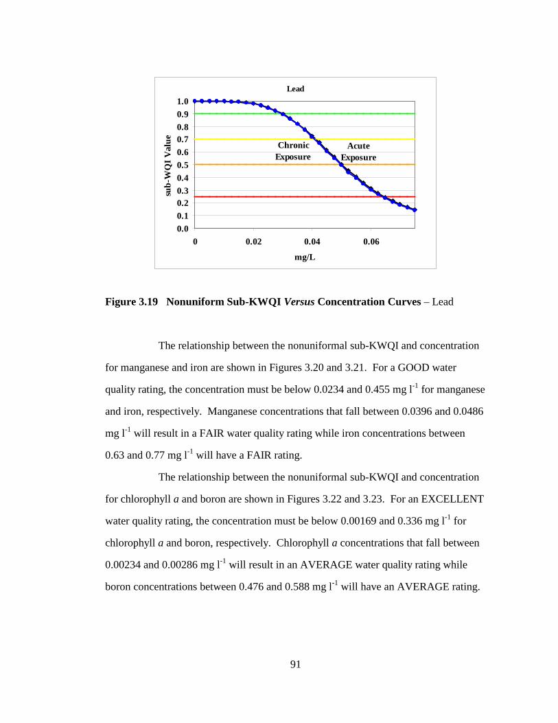
91

Lead

Acute Exposure

Chronic Exposure

0.00.10.20.30.40.50.60.70.80.91.0

0 0.02 0.04 0.06

mg/L

sub-

WQ

I Val

ue

Figure 3.19 Nonuniform Sub-KWQI Versus Concentration Curves – Lead


for manganese and iron are shown in Figures 3.20 and 3.21. For a GOOD water

quality rating, the concentration must be below 0.0234 and 0.455 mg l-1 for manganese

and iron, respectively. Manganese concentrations that fall between 0.0396 and 0.0486

mg l-1 will result in a FAIR water quality rating while iron concentrations between

0.63 and 0.77 mg l-1 will have a FAIR rating.


for chlorophyll a and boron are shown in Figures 3.22 and 3.23. For an EXCELLENT

water quality rating, the concentration must be below 0.00169 and 0.336 mg l-1 for

chlorophyll a and boron, respectively. Chlorophyll a concentrations that fall between

0.00234 and 0.00286 mg l-1 will result in an AVERAGE water quality rating while

boron concentrations between 0.476 and 0.588 mg l-1 will have an AVERAGE rating.

92

Manganese (domestic water)

0.00.10.20.30.40.50.60.70.80.91.0

0 0.01 0.02 0.03 0.04 0.05

mg/L

sub-

WQ

I Val

ue

Figure 3.20 Nonuniform Sub-KWQI Versus Concentration Curves – Manganese

Iron (Chronic Exposure)

0.00.10.20.30.40.50.60.70.80.91.0

0 0.1 0.2 0.3 0.4 0.5 0.6 0.7 0.8 0.9 1

mg/L

sub-

WQ

I Val

ue

Figure 3.21 Nonuniform Sub-KWQI Versus Concentration Curves – Iron

93

Chlorophyll a

0.00.10.20.30.40.50.60.70.80.91.0

0 0.001 0.002 0.003

mg/L

sub-

WQ

I Val

ue

Figure 3.22 Nonuniform Sub-KWQI Versus Concentration Curves – Chlorophyll a

Boron

0.00.10.20.30.40.50.60.70.80.91.0

0 0.1 0.2 0.3 0.4 0.5 0.6 0.7 0.8

mg/L

sub-

WQ

I Val

ue

Figure 3.23 Nonuniform Sub-KWQI Versus Concentration Curves – Boron

94

The final subindex, classified as unimodal, is based on the parameters

having an optimum value or range. The relationship between the unimodal sub-KWQI

and concentration for a single grab sample measurement and a daily average

measurement for dissolved oxygen is shown in Figure 3.24. The sub-KWQI values

decrease after reaching a concentration of 8.5 and 9.5 mg l-1 for a single

(instantaneous/grab) sample measurement and a daily average measurement,

respectively. Before reaching the optimum DO concentration, the sub-KWQI

increases at a slightly faster rate with increasing concentration for the grab sample

curve. However, for DO concentrations above the optimum value, the grab sample

sub-KWQI decreases at a slower rate than the daily average sub-KWQI. Grab sample

DO concentrations between 7.0 and 10.0 mg l-1 will have a water quality rating of

EXCELLENT while daily average DO concentrations between 8.5 and 11 mg l-1 will

receive an EXCELLENT. The DO curve starts to decrease after the optimum ranges

however, this can be explained. The natural upper level of solubility in water is

around 15 mg/L however this can be increases in particular cases. The additional

aeration could be the result from biological processes by autotrophic organisms (algae)

through photosynthesis. High levels of naturally occurring DO should be investigated

to determine if the water body has been taken over by too much plant biota (Biswas,

1997).

95

Dissolved Oxygen

Daily Average

Grab Sample

0.00.10.20.30.40.50.60.70.80.91.0

0 1 2 3 4 5 6 7 8 9 10 11 12 13 14 15

mg/L

sub-

WQ

I Val

ue

Figure 3.24 Unimodal Sub-KWQI Versus Concentration Curve - Dissolved Oxygen

The relationship between the unimodal sub-KWQI and concentration for

conductivity and pH are shown in Figures 3.25 and 3.26. Conductivity sub-KWQI

values increase to 1.00 for concentrations between 0 and 0.35 mS/cm, and decrease at

a slower rate for concentrations greater than 0.35 mS/cm. Changes in sub-KWQI

values for pH occur between the range of 4 and 11.5, reaching the maximum sub-

KWQI value (1.0) at pH 7.0. A rating of POOR is received for pH values below 5.8 or

above 9.0


temperature and fluoride are shown in Figures 3.27 and 3.28. The sub-KWQI value

for temperature increases at a slower rate for temperatures between 0° C and 20° C.

Temperatures above 20° C decrease in sub-KWQI values. Fluoride concentrations that

96

fall between 2.4 and 2.8 mg l-1 will result in an EXCELLENT rating while

concentrations below 1.43 and above 4.0 mg l-1 will have a POOR rating.

Conductivity

0.00.10.20.30.40.50.60.70.80.91.0

0 0.25 0.5 0.75 1 1.25 1.5

mS/cm

sub-

WQ

I Val

ue

Figure 3.25 Unimodal sub-KWQI Versus Concentration Curves – Conductivity

97

pH

0.00.10.20.30.40.50.60.70.80.91.0

0 2 4 6 8 10 12 14

sub-

WQ

I Val

ue

Figure 3.26 Unimodal sub-KWQI Versus Concentration Curves – pH

Temperature

0.00.10.20.30.40.50.60.70.80.91.0

0 5 10 15 20 25 30 35 40 45

°C

sub-

WQ

I Val

ue

Figure 3.27 Unimodal Sub-KWQI Versus Concentration Curves – Temperature

98

Fluoride

0.00.10.20.30.40.50.60.70.80.91.0

0.0 0.5 1.0 1.5 2.0 2.5 3.0 3.5 4.0 4.5 5.0 5.5 6.0

mg/L

sub-

WQ

I Val

ue

Figure 3.28 Unimodal Sub-KWQI Versus Concentration Curves – Fluoride


Total Dissolved Solids (TDS) and Total Suspended Solids (TSS) are shown in Figures

3.29 and 3.30. The sub-KWQI value for TDS and TSS concentrations of 0 mg l-1 is

0.76. Even though these water quality parameters fall under the unimodal sub-index

definition, the Delaware standards are based on a maximum concentration rather than

a range of acceptable concentrations. A POOR water quality rating occurs for TDS

concentrations above 39 mg l-1 and for TSS concentrations above 250 mg l-1.

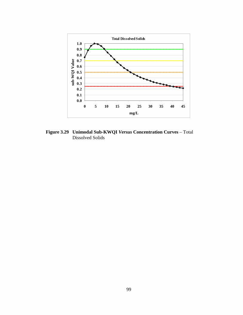
99

Total Dissolved Solids

0.00.10.20.30.40.50.60.70.80.91.0

0 5 10 15 20 25 30 35 40 45

mg/L

sub-

WQ

I Val

ue

Figure 3.29 Unimodal Sub-KWQI Versus Concentration Curves – Total Dissolved Solids

100

Total Suspended Solids

0.00.10.20.30.40.50.60.70.80.91.0

0 50 100 150 200 250 300

mg/L

sub-

WQ

I Val

ue

Figure 3.30 Unimodal Sub-KWQI Versus Concentration Curves – Total Suspended Solids

Model Development

A computer model was developed to perform the aggregation function that

computes the final, single, water quality index (KWQI) from the calculated sub-water

quality indices of individual water quality parameters. The KWQI can be calculated

by aggregating any number of different water quality parameters. The selection of

which water quality parameters to use to calculate the final index is usually based on

the type of water body under assessment, the intended water use, and the purpose of

the assessment. The model was created with a user friendly interface that would allow

for a variety of water quality parameters and parameter sets to be used for KWQI

aggregation.. This would allow the model to calculate a KWQI that could be used in

the future for the evaluation of the water quality of the Cool Run on the Newark

Research and Education Center Farm and for the assessment of the impacts that the

101

installed BMPs have on water quality in the Cool Run tributary. Because the model

was developed using Delaware’s water quality criteria, it could be used to assess any

surface water in the state. A brief overview describing the model functions and

application will be discussed. This will be followed by a breakdown of the individual

options that are available in the three parts of the model. It will conclude with a

simple example that will walk through one of the three options that are available in the

model.

Model Overview

The function of the model is to take many different parameter sub-indices

and create a single water quality index value that can determine the health of a stream

or the performance of a BMP. As stated in Chapter 1, having large amounts of data

and no basis to evaluate the data can cause a problem for environmentalists and policy

makers. The model is meant to help make sense of collected water data and to put it

into a presentable manner that can be use to describe processes in simplistic terms.

For instance, the model has been made with three main options. The first option will

provide an index value (KWQI) for a single set of parameters. The second option will

provide a way to directly compare two sets of data. For example, the model could

make a comparison of two different sample dates or a comparison of two points along

the same stream. The third option will allow a person to assess up to 8 different sets

of data at one time. These data sets can include monitoring data from single sampling

dates, monthly averages, yearly averages, or any other statistical evaluations (median

values for example).

When using the navigation buttons to switch between input pages, a

serious of options will be presented to guide the user through the KWQI. For

102

example, when clicking the navigation buttons, a window will pop up that will ask the

user to select from the following list of options: “continue to the page’’, “create your

own data set”, or “use one of the predefined parameter sets”. There are five groups of

predefined parameter sets that are broken down into the following categories: Water

Quality Standards and Criteria Sets, Manure Collection System Sets, Riparian Buffer

Zone Sets, Wetland Sets and Ponds/Basins Sets. Within each of these set categories,

there are 2-3 different options that are preprogrammed into the model. To make it

easier on the user, the list of water quality parameters that are used to calculate the

KWQI of each set is listed with the set name. The model also allows you to go back to

look at all the options before closing out the box by clicking the “Continue to Input

Page” button. When any of the preprogrammed parameter sets are chosen, there is

always the option of changing any of the parameters in the set. The purpose of the

predefined parameter sets it is to allow users with limited knowledge of the subject to

use this model for assessment of the impacts of particular BMPs with the Cool Run

tributary.

There are reset options built into the program to make clearing sheets

easier for the user. There are four options that are given when the “Reset Options”

button is clicked on the input or output pages. The first option is to clear only the

values that were entered on the input page. This is mainly for when the user runs the

same water quality parameters over and over again but changes the concentration of

the quality variables being entered into the model. The second option is to allow the

user to erase the values that are on the output page only. This is intended to be used

between runs to make sure that all the calculations are done correctly. It will also

provide an easy way to clear all the output from a specific run if a change in

103

parameters is desired. The third option clears the concentration of the quality values

from the input page and also clears the data that was outputted. This is mainly for

situations when the user is running many assessments and wants to make sure that all

the values are calculated correctly. The final option is to reset both the input and

output pages. The end result for this option is that the outputted data is cleared, the

quality variables are erased and all the parameter choices are cleared.

There are many applications where this model can be used. The main

intention for the development of the model was to create a way to evaluate the changes

that occur, if any, in the stream water quality in an agricultural setting where BMPs are

being implemented. The model can also be used to evaluate the health of any flowing

freshwater body, such as larger streams or rivers. This model can be applied to almost

any water body, even those outside of Delaware, as long as the criteria for the

parameters are adjusted for the area under study.

Model Options

The options that are available for use in the KWQI model are listed in

Table 3.8. Option 1 (Single Site) refers to sections of the model used with a single set

of data for a range of parameters. Option 2 (Side-by-Side) refers to sections of the

model used to compute up to two sets of data for a range of parameters. Option 3

(Spatial Estimation) refers to sections of the model where up to eight sets of data can

be done in a single run.

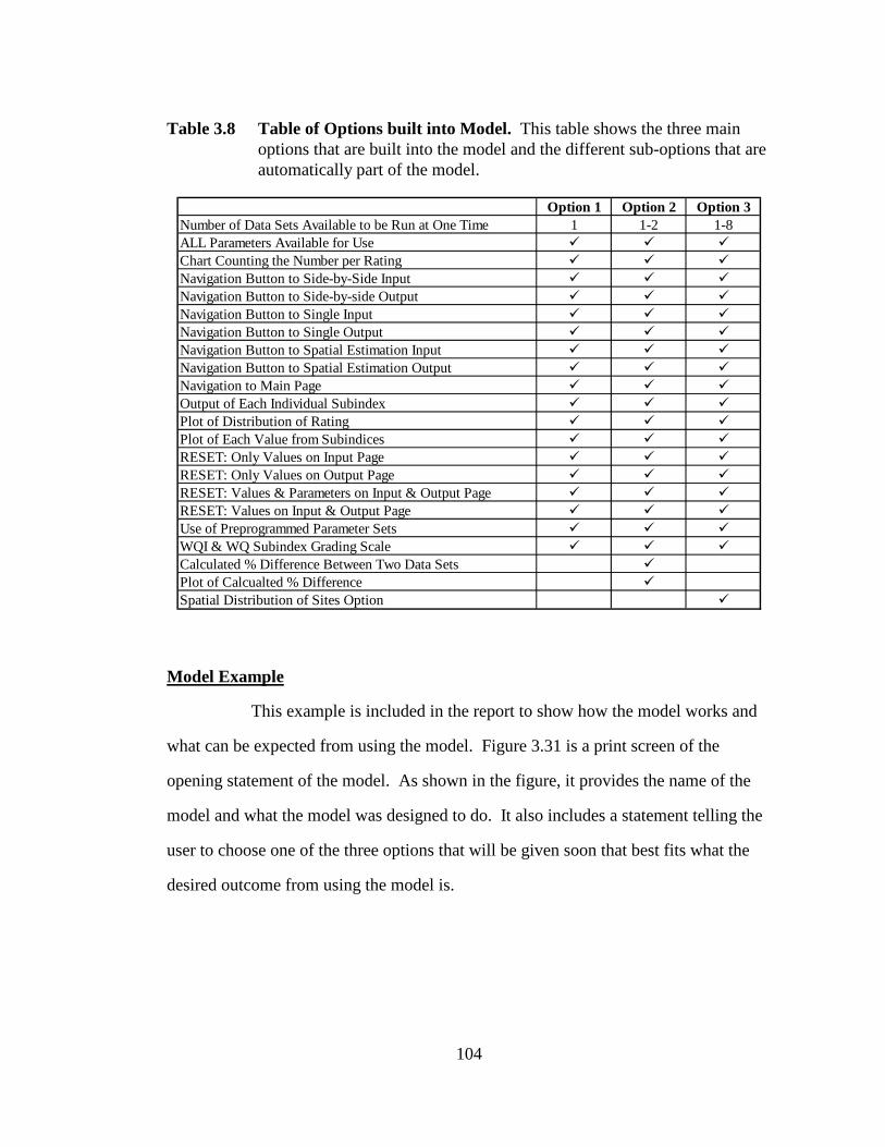
104

Table 3.8 Table of Options built into Model. This table shows the three main options that are built into the model and the different sub-options that are automatically part of the model.

Option 1 Option 2 Option 3Number of Data Sets Available to be Run at One Time 1 1-2 1-8ALL Parameters Available for Use Chart Counting the Number per Rating Navigation Button to Side-by-Side Input Navigation Button to Side-by-side Output Navigation Button to Single Input Navigation Button to Single Output Navigation Button to Spatial Estimation Input Navigation Button to Spatial Estimation Output Navigation to Main Page Output of Each Individual Subindex Plot of Distribution of Rating Plot of Each Value from Subindices RESET: Only Values on Input Page RESET: Only Values on Output Page RESET: Values & Parameters on Input & Output Page RESET: Values on Input & Output Page Use of Preprogrammed Parameter Sets WQI & WQ Subindex Grading Scale Calculated % Difference Between Two Data Sets Plot of Calcualted % Difference Spatial Distribution of Sites Option

Model Example

This example is included in the report to show how the model works and

what can be expected from using the model. Figure 3.31 is a print screen of the

opening statement of the model. As shown in the figure, it provides the name of the

model and what the model was designed to do. It also includes a statement telling the

user to choose one of the three options that will be given soon that best fits what the

desired outcome from using the model is.

105

Figure 3.31 KWQI Model - Opening Screen of Kiliszek WQI Worksheet. This is a screen shot of the opening screen providing some background information on the KWQI and instructing the user to read the options list to make best use of the options available.

After clicking the continue button, the user will then see the print screen

that is in Figure 3.32. To help the user navigate to the part of the model that is most

useful to them, each option is described in detail. The description for each option

includes what types of data sets were intended to be used to calculate the final index.

The content of the output page that is automatically generated with each run of the

model is given in list form.

106

Figure 3.32 KWQI Model - Main Menu Options. This is a screen shot of the options page within the model. It shows the options and cases for each option as well as the output included after the model is ran.

For this example, the option that was chosen was the “Side by Side

Evaluation”. Once the button is clicked, the model will automatically direct you to the

“Side by Side Evaluation” tab where the dialog box (Figure 3.33) will appear on top of

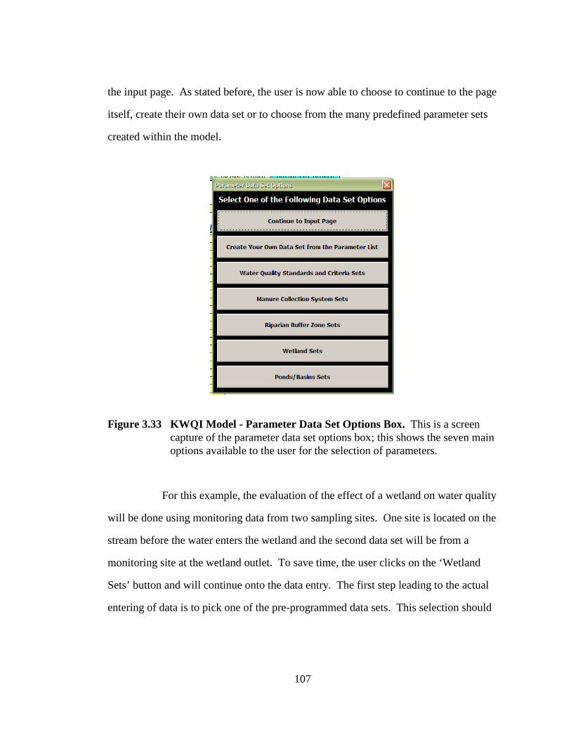
107

the input page. As stated before, the user is now able to choose to continue to the page

itself, create their own data set or to choose from the many predefined parameter sets

created within the model.

Figure 3.33 KWQI Model - Parameter Data Set Options Box. This is a screen capture of the parameter data set options box; this shows the seven main options available to the user for the selection of parameters.

For this example, the evaluation of the effect of a wetland on water quality

will be done using monitoring data from two sampling sites. One site is located on the

stream before the water enters the wetland and the second data set will be from a

monitoring site at the wetland outlet. To save time, the user clicks on the ‘Wetland

Sets’ button and will continue onto the data entry. The first step leading to the actual

entering of data is to pick one of the pre-programmed data sets. This selection should

108

be based on how rigorous the evaluation will be. For all the data sets except the

Manure Collection System Sets, there are at least three options provided. The first

option is always the one that contains the smallest number of parameters. This is

referred to as the minimum number of parameters that should be evaluated when

assessing the BMP. It will provide a very basic parameter set that will only use the

parameters that are most commonly affected by the BMP in question. The general sets

combine the minimum data set with additional parameters that would be associated

with the general health of the water body. The final choice is defined as the maximum

which includes any additional water quality parameters that could be affected by the

BMP. Each popup set dialog box includes a ‘GO BACK’ button so that if the user is

unsure of which set they would like to use, they can easily change their selection.

Figure 3.34 shows the parameter sets that have been preprogrammed for wetland

evaluation. This example uses the minimum parameter set for evaluation of wetland

efficiency for water quality improvement.

109

Figure 3.34 KWQI Model - Wetland Parameter Sets. This screen shot of the model shows one of the seven parameter data set options available. From this you can see that there are multiple options available and that the parameters for each option are listed.

After choosing the parameter set button, the box will close and the user

must click the ‘Continue to Input Page’ button to input the data. The print screen in

Figure 3.35 shows the parameters that were entered into the parameter spaces

automatically by choosing that option. The user may also change the parameters at

this point. Each of the parameter input spaces have a drop box built into them that

contains a list of all the parameters that are available for use in this model. The drop

box menu is shown in Figure 3.36.

Test for 9 font

110

Figure 3.35 KWQI Model - Entered Parameters and Drop Down Menu – Automated selection using the models predetermined parameter set.

Figure 3.36 KWQI Model - Entered Parameters and Drop Down Menu – Parameter selection using the dropdown menu.

111

The user will then have to enter the concentration values of the selected

parameters into the program and define how many parameters are being used. To help

keep track of the number of parameters entered, a counter has been added to the page

view. It is important to correctly input the total number of parameters used because

the equation that calculates the final KWQI value is dependant upon this number. This

will also be useful when evaluating a greater number of parameters. After filling in

the values, as shown in Figure 3.37, the user will then push the “Click to Run

Analysis” button (Figure 3.38). This appears on every input sheet and will run the

program, output the data to another work sheet within the model and then switch the

view to the newly created output page.

Figure 3.37 KWQI Model - Completed Example Input. This screen shot of the model provides an example of the input page from the side by side comparison of four parameters.

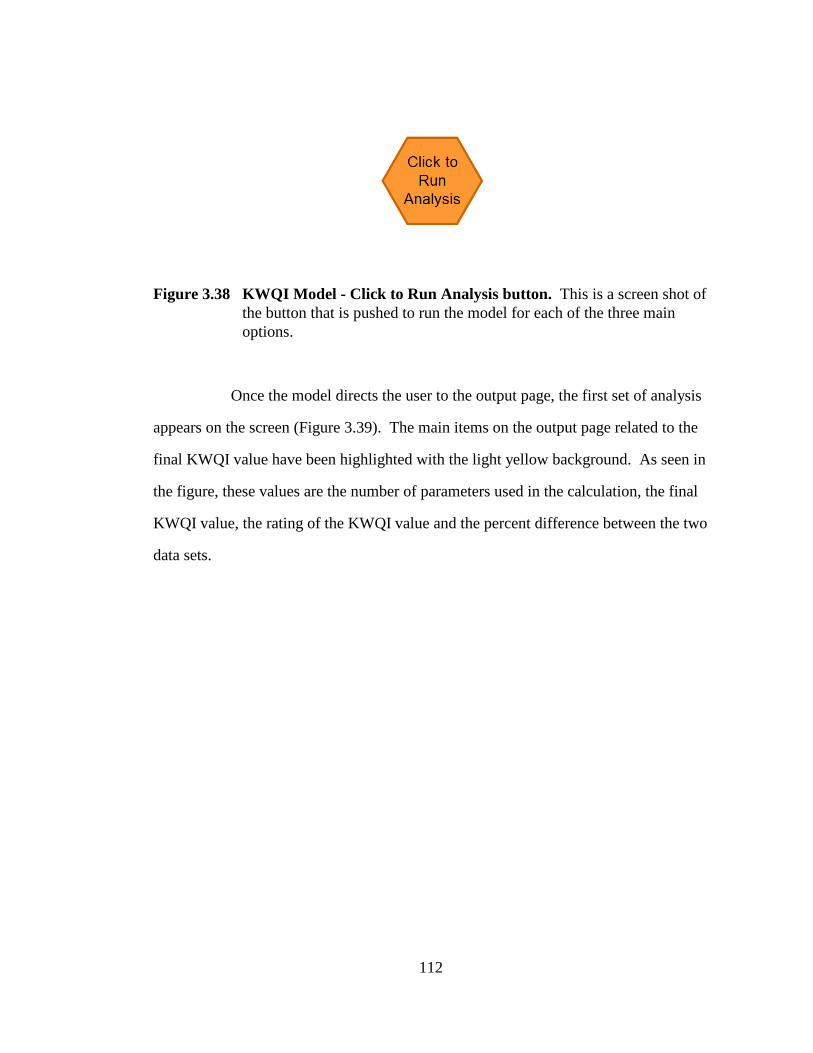
112

Figure 3.38 KWQI Model - Click to Run Analysis button. This is a screen shot of the button that is pushed to run the model for each of the three main options.

Once the model directs the user to the output page, the first set of analysis

appears on the screen (Figure 3.39). The main items on the output page related to the

final KWQI value have been highlighted with the light yellow background. As seen in

the figure, these values are the number of parameters used in the calculation, the final

KWQI value, the rating of the KWQI value and the percent difference between the two

data sets.

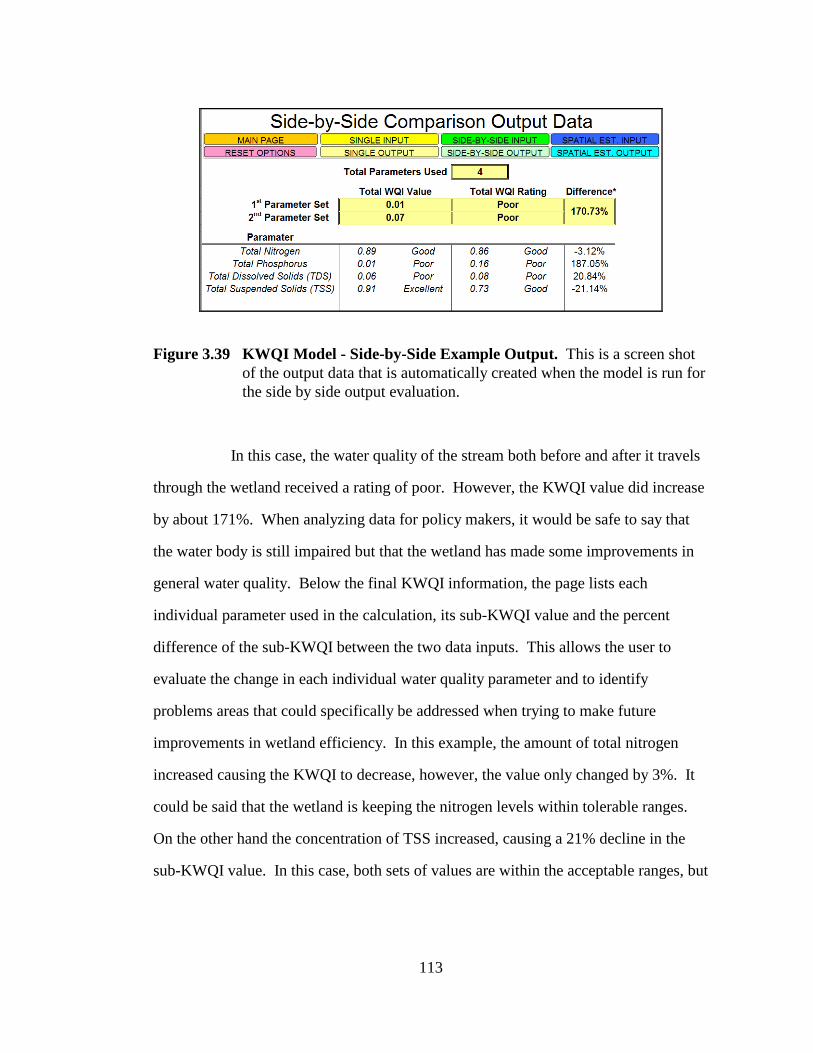
113

Figure 3.39 KWQI Model - Side-by-Side Example Output. This is a screen shot of the output data that is automatically created when the model is run for the side by side output evaluation.

In this case, the water quality of the stream both before and after it travels

through the wetland received a rating of poor. However, the KWQI value did increase

by about 171%. When analyzing data for policy makers, it would be safe to say that

the water body is still impaired but that the wetland has made some improvements in

general water quality. Below the final KWQI information, the page lists each

individual parameter used in the calculation, its sub-KWQI value and the percent

difference of the sub-KWQI between the two data inputs. This allows the user to

evaluate the change in each individual water quality parameter and to identify

problems areas that could specifically be addressed when trying to make future

improvements in wetland efficiency. In this example, the amount of total nitrogen

increased causing the KWQI to decrease, however, the value only changed by 3%. It

could be said that the wetland is keeping the nitrogen levels within tolerable ranges.

On the other hand the concentration of TSS increased, causing a 21% decline in the

sub-KWQI value. In this case, both sets of values are within the acceptable ranges, but

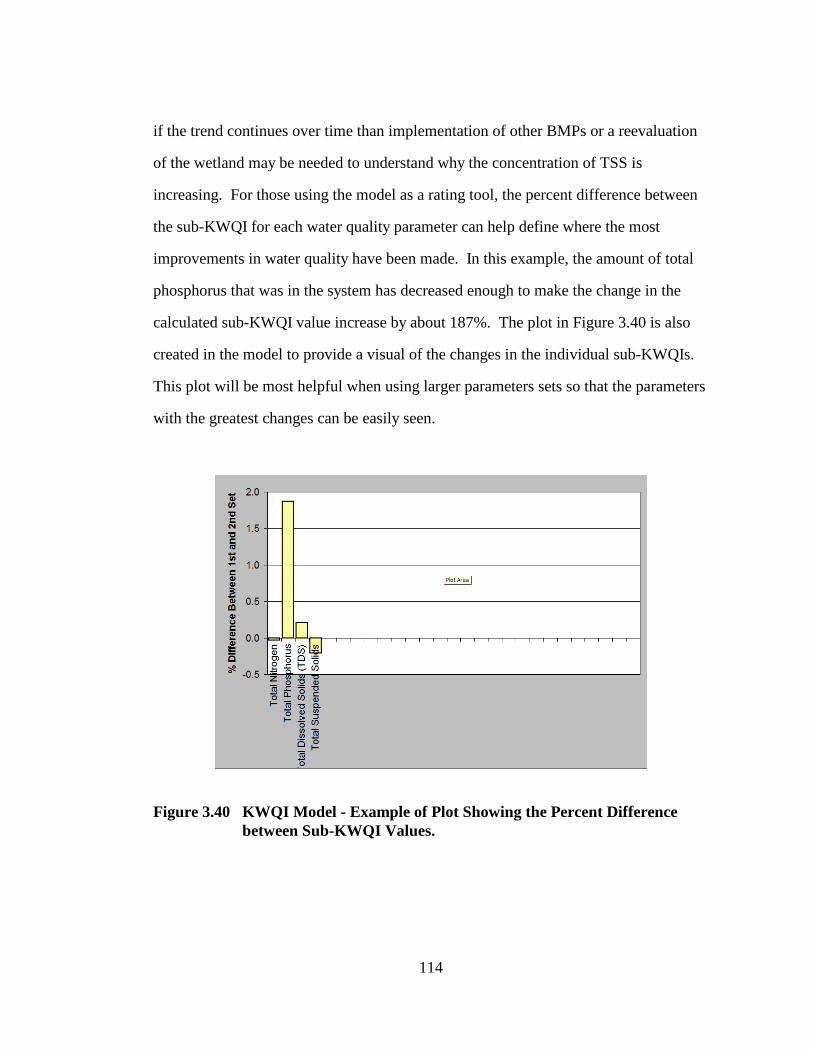
114

if the trend continues over time than implementation of other BMPs or a reevaluation

of the wetland may be needed to understand why the concentration of TSS is

increasing. For those using the model as a rating tool, the percent difference between

the sub-KWQI for each water quality parameter can help define where the most

improvements in water quality have been made. In this example, the amount of total

phosphorus that was in the system has decreased enough to make the change in the

calculated sub-KWQI value increase by about 187%. The plot in Figure 3.40 is also

created in the model to provide a visual of the changes in the individual sub-KWQIs.

This plot will be most helpful when using larger parameters sets so that the parameters

with the greatest changes can be easily seen.

Figure 3.40 KWQI Model - Example of Plot Showing the Percent Difference between Sub-KWQI Values.

115

The plot in Figure 3.41 is adapted for use in all three model options and

was added to the model to show the distribution of sub-KWQI values per parameter.

Similar to the percent different plot, it can be used to quickly identify the parameters

that are the most impaired among the parameter set run. Using this plot, the reason

behind low KWQI values can be justified. In this example, the TP and TDS sub-

KWQIs were very low for both sets of data compared to the sub-KWQIs for TN and

TSS. Since the KWQI uses an aggregation method that does not mask the lower

scoring subindices with averages, these low scoring parameters caused the final KWQI

value to be low.

Figure 3.41 KWQI Model - Example of Output Plot of Side by Side Comparison of Sub-KWQI Values

Another output set that is included in the model assessment can be seen in

Figure 3.42. The green section of the table in Figure 3.42 shows the rating scale and

116

the associated WQI rating scale values. The blue section of the figure shows a

breakdown of the five sub-KWQI ratings achieved and lists the number of parameters

falling within that sub-index rating. This is available for all three of the model

options.

Figure 3.42 KWQI Model - Example of Rating Scale Table and Number of Parameters per sub KWQI Rating

A plot of the sub-index ratings is generated to graphically show the distribution of the

number of parameter sub-indices falling within each of the five rating categories

(Figure 3.43).

117

Figure 3.43 KWQI Model - Example of Chart of Sub Index Rating Distribution

The most important feature of a user-friendly model is the ability to

navigate with ease within the model pages. A tool bar was created to add this feature

(Figure 3.44). The tool bar consists of color coded tabs that allow the user to switch

between any of the pages by clicking the desired destination. If the user would like to

change which main section of the model they are in, going back to the main page will

allow them to re-read the option descriptions and decide which one to use.

Figure 3.44 KWQI Model - Navigation Tool Bar. This is a screen shot of the navigation tool bar that is intended to be used while using the model. The user will scroll over and click the buttons to activate them.

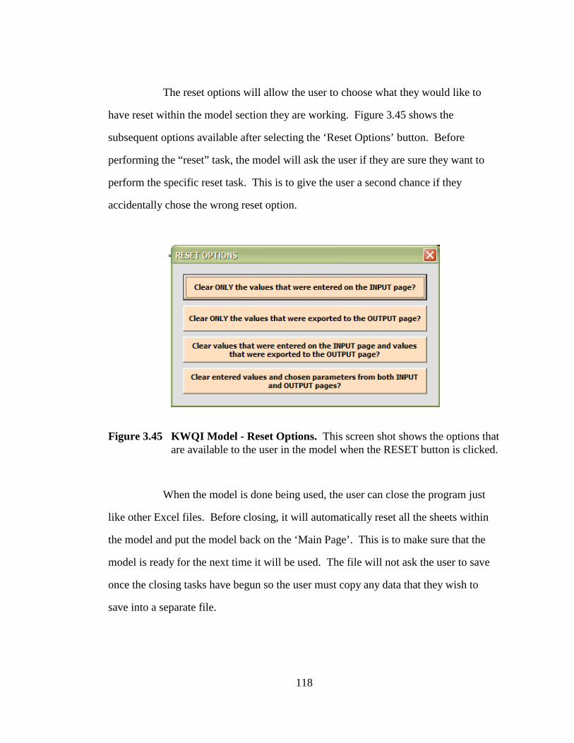
118

The reset options will allow the user to choose what they would like to

have reset within the model section they are working. Figure 3.45 shows the

subsequent options available after selecting the ‘Reset Options’ button. Before

performing the “reset” task, the model will ask the user if they are sure they want to

perform the specific reset task. This is to give the user a second chance if they

accidentally chose the wrong reset option.

Figure 3.45 KWQI Model - Reset Options. This screen shot shows the options that are available to the user in the model when the RESET button is clicked.

When the model is done being used, the user can close the program just

like other Excel files. Before closing, it will automatically reset all the sheets within

the model and put the model back on the ‘Main Page’. This is to make sure that the

model is ready for the next time it will be used. The file will not ask the user to save

once the closing tasks have begun so the user must copy any data that they wish to

save into a separate file.

119

Model Design Assessment: Comparing Kiliszek WQI Ratings to Harrell (2002) Grading Scale

The purpose of research done by Harrell (2002) was to update a water

quality assessment method developed by student researchers funded by the UD Water

Resources Agency (UDWRA). The goal of Harrell’s project was to update and utilize

the older water quality rating system so that it would link stream health to land use.

The end result was an updated report card on stream health that could be applied to

any sampling site within the UDEW. The report card was meant to be simple enough

so that changes could easily be made.

There were 18 water quality parameters monitored for the report card

assessment project (Harrell, 2002). Only 9 of those parameters were utilized in the

current research. The parameters that were not used from Harrell’s (2002) work are

alkalinity, chloride, chlorine, hardness, phosphate, turbidity, odor, sheen, and

hydrocarbon. Parameters that were used include ammonia, chromium, copper,

dissolved oxygen, BOD, iron, nitrate, pH, and conductivity.

The first step that was done to test the model was to make a comparison of

the two grading scales. The two grading scales can be seen in Table 3.9, the Harrell

scale has been related to the KWQI scale to compare the rating ranges. From the table

it is clear that the distribution is different between the two scales. The Harrell states

that any value below a 0.40 will receive a rating of POOR where the KWQI value

must be below 0.25. The EXCELLENT rating scales are similar to each other only

differing by 0.03 points in both scales. The range for each of the individual ratings is

approximately the same size but as stated previously the main difference is the score in

which the quality variable will receive a rating of POOR.

120

Table 3.9 Rating Range Guides for Harrell (2002) and Kiliszek WQI. This table shows the distribution of the rating scales for the Harrell method and the KWQI.

Harrell Kiliszek WQIExcellent 1 .00 - 0.88 1.00 - 0.91

Good 0.87 - 0.65 0.90 - 0.71Average - 0.70 - 0.51

Fair 0.65 - 0.40 0.50 - 0.25Poor <0.40 <0.25

Table 3.10 compares the parameter scoring guides for the Harrell (2002)

and the KWQI models. There are many similarities between the two grading systems

which makes them comparable. However, there are some major differences between

the scales as well.

The first similarity is that both model rating scales use excellent, good, fair

and poor. The KWQI model has one additional rating category, which is average,

falling in between good and fair. Another similarity is that there is no weighting scale

for each parameter, they are all equal and carry equal weight when the total rating is

calculated. This is one of the points that Swamee and Tyagi (2000 & 2007) stressed in

their research, i.e., weighting will skew the grading scale. Although, using a strict

average of individual parameter ratings will mask the lower scoring parameters

resulting in a rating that is not representative of the entire picture.

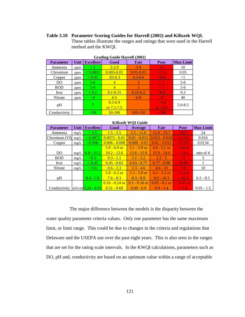
121

Table 3.10 Parameter Scoring Guides for Harrell (2002) and Kiliszek WQI. These tables illustrate the ranges and ratings that were used in the Harrell method and the KWQI.

Parameter Unit Excellent Good Fair Poor Max LimitAmmonia ppm < 1 2-2.9 3-4 >5 10Chromium ppm < 0.0003 0.003-0.01 0.01-0.03 >0.04 0.05

Copper ppm < 0.03 .03-0.3 0.3-0.6 >0.6 <1DO ppm 5-6 4 3 < 2 5-6

BOD ppm 5-6 4 3 < 2 5-6Iron ppm < 0.1 0.1-0.15 0.15-0.2 >0.2 0.3

Nitrate ppm <4 4-5 6-8 >8 40

pH 7 6.5-6.9or 7.1-7.5

< 6.0 or >8.0 5.0-8.5

Conductivity >50 50-100 100-150 >200

Parameter Unit Excellent Good Average Fair Poor Max LimitAmmonia mg/L < 1.5 1.5 - 5.5 5.5 - 11.0 11.0 - 23.7 >23.7 24

Chromium (VI) mg/L < 0.0072 0.0072 - 0.01 0.01 - 0.012 0.012 - 0.016 >0.016 0.016Copper mg/L >0.006 0.006 - 0.008 0.008 - 0.01 0.01 - 0.013 >0.013 0.0134

DO mg/L 6.9 - 10.25.9 - 6.9 or10.2 - 12.6

5.1 - 5.9 or12.6 - 15.9

4.0 - 5.1 or15.9 - 24.6

< 4.0 or> 24.6 min of 4

BOD mg/L <0.3 0.3 - 1.1 1.1 - 2.2 2.2 - 5 >5 5Iron mg/L < 0.45 0.45 - 0.63 0.63 - 0.77 0.77 - 0.98 >0.98 1

Nitrate mg/L < 0.6 0.6 - 2.3 2.3 - 4.6 4.6 - 10 >10 10

pH 6.4 - 7.65.8 - 6.3 or

7.6 - 8.35.3 - 5.8 or

8.3 - 8.94.3 - 5.3 or8.9 - 10.3

< 4.3 or> 10.3 6.5 - 8.5

Conductivity mS/cm 0.24 - 0.510.16 - 0.24 or

0.51 - 0.690.1 - 0.16 or

0.69 - 0.90.05 - 0.1 or

0.9 - 1.4< 0.05 or

> 1.4 0.05 - 1.5

Kiliszek WQI Guide

Grading Guide Harrell (2002)

The major difference between the models is the disparity between the

water quality parameter criteria values. Only one parameter has the same maximum

limit, or limit range. This could be due to changes in the criteria and regulations that

Delaware and the USEPA use over the past eight years. This is also seen in the ranges

that are set for the rating scale intervals. In the KWQI calculations, parameters such as

DO, pH and, conductivity are based on an optimum value within a range of acceptable

122

values. The Harrell (2002) rating process uses only a single range for DO and

conductivity without optimum values.

Table 3.11 compares the final ratings calculated for the individual water

quality parameters using both models based on the values provided in Harrell (2002).

There were five sites that Harrell (2002) used that that were related to sites used on the

UDAESF. Two sample locations were the same in both projects, CP3CR (known as

UDAESF Site 2) and CP2CR (known as UDAESF Site 5). Sample locations CP6T3

(known UDAESF Site 3) and CP5T2 (known as UDAESF Site 4) were taken just

north of the Amtrak railroad tracks were this project sampled south of the railroad

tracks. The final similar sample location was CP4T1 (known as UDAESF Site 7/8)

which is located at a stormwater grate that is between Sites 7 and 8 on the farm.

123

Table 3.11 Kiliszek WQI vs Harrell (2002) Grading System. This table compares the KWQI Subindex values to the Harrell Sub-rating values. The overall rating from both the KWQI and Harrell method are also shown with the respective rating scales.

sub- sub- sub- sub- sub-Parameter WQI Har WQI Har WQI Har WQI Har WQI HarAmmonia G G E E E E E E G FChromium E E E E E E E E E E

Copper E E E E E E E E P PDO F E G E P P P G E E

BOD5 E P G F E P E P G FIron E E P P E E F P P P

Nitrate P P P P A E P P E EpH G F F F A G A G E E

Conductivity A P P E n/a n/a F P F P

Value Determined by Indiviudal System {WQI 0 - 1.0} {Harrell 1 - 4 }WQI 0.24 0 0.03 0.12 0

Harrell 2.67 2.89 3.13 2.44 2.33

OVERALL P F P G P G P F P FE = Excellent G = Good A = Average F = Fair P = Poor

Site 7/8(CP4T1)

Site 2 (CP3CR)

Site 3(CP6T3)

Site 4(CP5T2)

Site 5(CP2CR)

Despite the differences in criteria limits used in the two models to calculate the sub-

indices and their associate ratings, many of the individual water quality parameter

ratings were the same for the two models. The ratings developed by each model for

chromium and copper concentrations were the same for all 5 monitoring sites. The

concentrations of Cr found in the water at the monitoring sites were low enough to

earn a rating of excellent. Surface water concentrations of copper received an

excellent rating at all the sites except for Site7/8 where elevated copper levels resulted

in a rating of poor. The rankings calculated by both models for ammonia differed only

at Site 7/8. Ammonia levels were considered excellent at sites 3, 4, and 5. Site 2

earned a rating of good for ammonia concentration by both models. The rating

124

calculated for ammonia concentration at Site 7/8 was good and fair for the KWQI

model and the Harrell model, respectively. Similarly, the rankings calculated by both

models for iron differed only at Site 5. Iron levels for considered excellent at sites 2

and 4 but poor at sites 3 and 7/8. The rating calculated for iron concentration at Site 5

was fair and poor for the KWQI model and the Harrell model, respectively. The

rankings calculated by both models for nitrate differed only at Site 4. Nitrate levels

were considered excellent at site 7/8 but poor at sites 2, 3 and 5. The rating calculated

for nitrate concentration at Site 4 was average and excellent for the KWQI model and

the Harrell model, respectively. The rankings calculated by both models for pH agreed

only at Sites 3 (FAIR) and 7/8 (EXCELLENT). At Sites 4 and 5, the ratings for pH

were average and good for the KWQI model and the Harrell model, respectively. At

site 2, the rating calculated for pH was good and fair for the KWQI model and the

Harrell model, respectively.

These differences could be attributed to the lack of 5th ranking in the

Harrell (2002) model. The differences could also be explained by the variation in

parameters limits and the division of the limits over the two different rating scales.

The rankings calculated by both models for DO agreed only at Sites 4

(POOR) and 7/8 (EXCELLENT). At Site 3, the ratings for DO were good and

excellent for the KWQI model and the Harrell model, respectively. At Sites 2 and 5,

the rating calculated for DO differed by at least two ranking categories. The DO

criteria used in the KWQI model had a range of acceptable concentrations where

concentrations greater than 24.6 or less than 4.0 mg l-1 would receive a rating of poor.

In the Harrell model, only concentrations below 2 mg l-1 would receive a rating of

poor.

125

The rankings calculated by both models for conductivity did not agree for

any of the monitoring sites. However, the rankings for Sites 2, 5 and 7/8 only varied

by one ranking category. The ratings for conductivity calculated by both models for

Site 3 were poor and excellent for the KWQI model and the Harrell model,

respectively. This difference was directly related to the concentration limits used in

the calculation. The KWQI model allows for a wider range of acceptable values in

conductivity. However, the data point in this case still fell outside the acceptable

range resulting in the poor rating.

The ratings developed by each model for BOD were different for all 5

monitoring sites. The BOD had three similar situations where the KWQI indicated

that the BOD was within the tolerable limit but that the Harrell method indicated that

the parameter was not. This was due to differences in the relationship between the

sub-index value and the concentration of BOD. In the KWQI model, the higher the

BOD concentration, the lower the sub-KWQI value it received. The Harrell model

indicated that the higher the BOD concentration, the higher the ranking values, where

the opposite is true in the KWQI model. Normally, a higher BOD concentration

indicates higher levels of organic compounds present in the water, which would tie up

the oxygen during biological and chemical degradation, thus resulting in lower water

quality.

The overall rankings calculated by the models were very different for all

of the 5 monitoring locations. All five sites received a KWQI rating of poor due to the

fact that at each of the sites, there were water quality parameters that received a sub-

KWQI value of zero or near zero. Using the Harrell (2002) method, Sites 2, 3, 4, 5,

and 7/8 received the grades of fair, good, good, fair and fair, respectively. The major

126

difference between the two models is in the type of aggregation equation used to

calculate the final index and corresponding rating value. Harrell (2002) averaged all

the values that were assigned to each parameter. Given that the scale went from 1 to 4,

where 1 was poor and 4 was excellent, your total grade would be between 1 and 4.

Simply averaging the values may cause the poorly rated parameters to be masked by

the high ranking scores thereby resulting in an overall water quality rating higher than

expected. The KWQI model uses an aggregation equation developed by Swamee and

Tyagi (2000 & 2007) that does not weight the individual parameters but does not let

parameters with low sub-index values be masked by parameters receiving high sub-

index values. Therefore the KWQI model will indicate impairment in stream health

when the concentration of only one water quality parameter falls below the established

criteria. A single, very low sub-index value can cause the final KWQI to fall within

the poor rating category. For this reason, the KWQI model program shows the

individual parameter sub-indices and ratings as well as the overall index and rating

value. The model was designed to function as a tool to identify problems in stream

health and to identify which individual water quality parameters have the greatest

influence on the overall rating.. The model’s assessment allows the user to monitor

the stream’s changes in overall water quality as well as the change in concentration of

each individual monitored parameter.

Selection of Parameter Sets for KQWI Model Assessments

A summary of the parameter sets is shown in Table 3.12 indicating the

number and type of parameters used in each of the different assessment scenarios.

The first section of parameter sets in the table is based on the DWQS for

fresh water and is used for assessments of general fresh water stream health. This set

127

contains 6 basic parameters: temperature, DO, pH, turbidity and coliform bacteria.

The second set of parameters will include the DWQS set with the addition of the

Delaware Water Quality Criteria for the Protection of Aquatic Life (DWQCPAL). The

additional parameters include: aluminum, ammonia, arsenic, cadmium, chromium,

copper, lead, nickel and zinc. The third set of parameters will combine the DWQS and

the DWQCPAL in addition to the Delaware Water Quality Criteria for the Protection

of Human Health (DWCPHH), adding nitrate to parameter set. The fourth set of

parameters includes the DWQS, DWQCPAL and the DWCPHH with the addition of

the USEPA criteria for nutrients; additional parameters include total phosphorus, total

nitrogen and chlorophyll a. The fifth parameter set includes all 22 parameters that

were monitored in the Cool Run. The sixth set in this section will include only

parameters the USEPA state as early indicators of stream impairment, these are nitrate,

total phosphorus, turbidity and chlorophyll a.

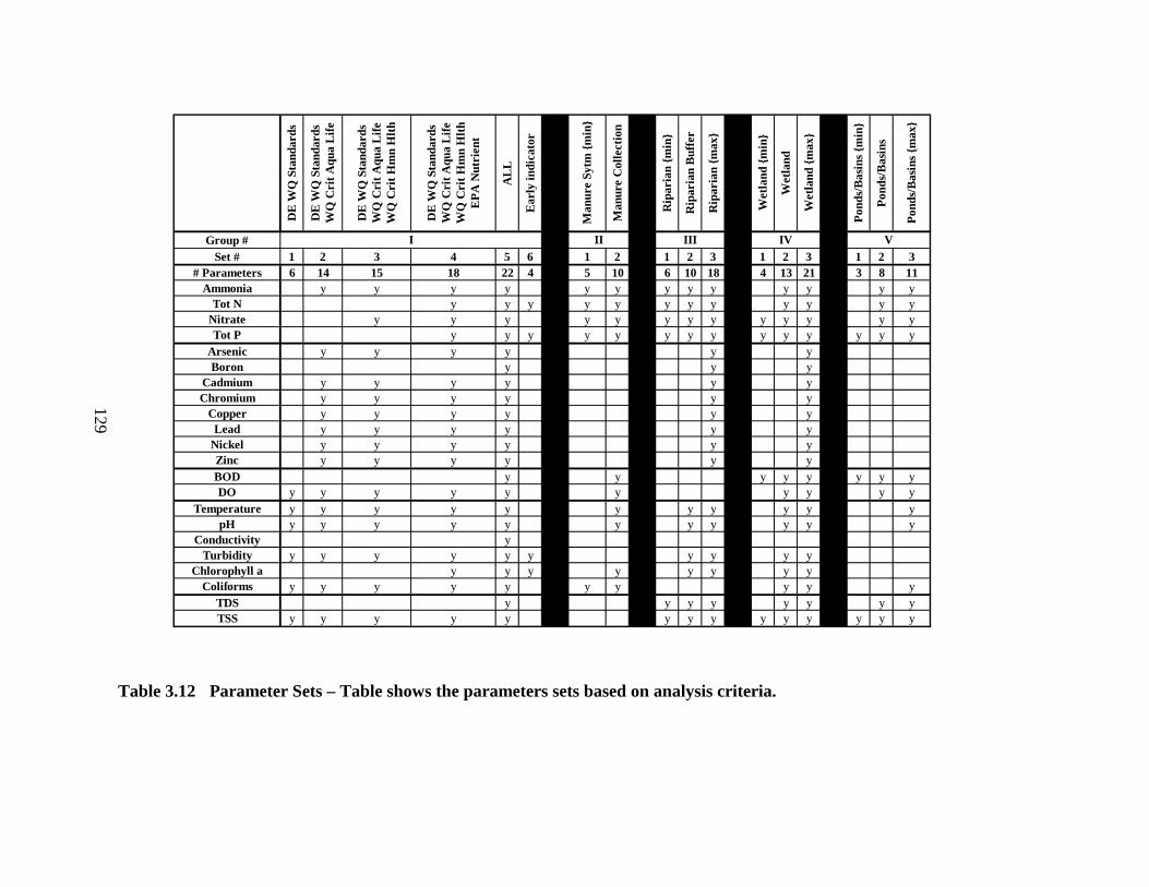
DE

WQ

Sta

ndar

ds

DE

WQ

Sta

ndar

dsW

Q C

rit A

qua

Life

DE

WQ

Sta

ndar

dsW

Q C

rit A

qua

Life

WQ

Cri

t Hm

n H

lth

DE

WQ

Sta

ndar

dsW

Q C

rit A

qua

Life

WQ

Cri

t Hm

n H

lthE

PA N

utri

ent

AL

L

Ear

ly in

dica

tor

Man

ure

Sytm

{min

}

Man

ure

Col

lect

ion

Rip

aria

n {m

in}

Rip

aria

n B

uffe

r

Rip

aria

n {m

ax}

Wet

land

{min

}

Wet

land

Wet

land

{max

}

Pond

s/B

asin

s {m

in}

Pond

s/B

asin

s

Pond

s/B

asin

s {m

ax}

Group #Set # 1 2 3 4 5 6 1 2 1 2 3 1 2 3 1 2 3

# Parameters 6 14 15 18 22 4 5 10 6 10 18 4 13 21 3 8 11Ammonia y y y y y y y y y y y y y

Tot N y y y y y y y y y y y yNitrate y y y y y y y y y y y y yTot P y y y y y y y y y y y y y y

Arsenic y y y y y yBoron y y y

Cadmium y y y y y yChromium y y y y y y

Copper y y y y y yLead y y y y y y

Nickel y y y y y yZinc y y y y y yBOD y y y y y y y yDO y y y y y y y y y y

Temperature y y y y y y y y y y ypH y y y y y y y y y y y

Conductivity yTurbidity y y y y y y y y y y

Chlorophyll a y y y y y y y yColiforms y y y y y y y y y y

TDS y y y y y y y yTSS y y y y y y y y y y y y y y

VI II III IV

Table 3.12 Parameter Sets – Table shows the parameters sets based on analysis criteria.

129

129

The other assessment groups were designed for the model in order to

evaluate the impacts on water quality of the Cool Run after implementation of the

different BMPs on the NRECF. The second group was designed to assess the effects

of the Manure Collection System, which was installed in order to reduce the amount of

nutrients and coliform bacteria in surface runoff entering the stream. The five

parameters chosen for the first set in this assessment group include ammonia, total

nitrogen, nitrate, total phosphorus and coliform bacteria. The second set of parameters

in this group includes the previous five parameters with the addition of BOD, DO,

temperature, pH and chlorophyll a. These parameters were added to help characterize

the overall health of the stream because of the indirect effects that manure leachate

components may have on geochemical processes that could result in changes in their

concentrations.

The third group of parameter sets was designed to assess the effects of

riparian buffer zones on stream water quality. Buffer zones can be used to help control

bank erosion, remove nutrients and prevent sediment from entering the stream. The

minimum number of parameters that were chosen to rate the effect of the riparian

buffers included six parameters; ammonia, total nitrogen, nitrate, total phosphorus,

TDS and TSS (Group III - Set 1). The set 2 in this group included the previous set as

well as the addition of temperature, pH, turbidity and chlorophyll a. These parameters

were added to help determine the overall health of the stream in addition to the

parameters directly influenced by buffer zones. The final parameter set (Set 3) in this

group adds 8 different metals. The metals include arsenic, boron, cadmium,

chromium, copper, lead, nickel and zinc. The addition of the metals was included to

130

help determine if the vegetation along the stream is able to uptake the metals as

potential micronutrients for growth from the water as it moves through the system.

The fourth group of parameter sets was designed to assess the effect a

wetland has on the water as it flows through. Wetlands are designed to remove the

total amount of nitrogen, settle out solids and reduce the amount of phosphorus in the

water moving through the system. The minimum parameter set that is to be used for

the evaluation of the wetland includes 4 parameters; total nitrogen, total phosphorus,

BOD, and TSS (Group IV - Set 1). The second set of parameters in this group was

designed to determine more specifically which nitrogen species have been degraded in

the wetland by the addition of ammonia and nitrate; turbidity has also been added. To

check on the general health of the wetland, DO, temperature, pH, chlorophyll a,

coliform bacteria and TDS were added to this set. The final parameter set in this

group (Group IV - Set 3) includes all of the parameters from the previous set with the

addition of the metals arsenic, boron, cadmium, chromium, copper, lead, nickel and

zinc. Similar to the riparian buffer zone, the plants within and surrounding the wet

areas of the wetland should take up some of the metals as micronutrients.

The fifth and final group of parameters that are listed in the Table 3.12

were designed to assess the productivity of a pond/storm water basin. These basins are

typically known for their ability to decrease the amount of phosphorus and BOD and

for providing a place for sedimentation to occur. The first set of parameters in this

group only evaluates the pond’s effect on phosphorus, BOD and TSS concentrations.

These parameters are very limited and provide a very small but specific picture of what

is actually occurring in the stream. The second set of parameters in this group adds

ammonia, total nitrogen, nitrate, DO and TDS to the previous parameters. This will

131

provide a little bit more information about the general health of the pond/basin. The

final set of parameters (Group V - Set 3) use all the above listed parameters and adds

temperature, pH and coliform bacteria. These three parameters were added because

they are considered indicators of stream health for fresh waters.

The KWQI Worksheet Model was used to calculate the KWQI values

using the average 2009 monitoring data for Site 4. The individual sub-index values for

all 22 parameters previously listed in Table 3.12 are shown in Table 3.13. This was

done to show the range of values that would be used in the aggregation process that

determines the final KWQI for the different parameter sets. It is clear from the table,

that the sub- KWQI values range from 0.07 to 1.00. Although there were many

“Excellent” ratings in this set, it also contained parameters that received a low rating

of “Poor”. This set was chosen to show the impact of choosing different parameters

for aggregation on the final KWQI value. This set of parameters was used to

determine the effects on the addition of parameters for all the different groups of

parameter sets.

Once the subindices were calculated for each of the 22 parameters, the

KWQIs for each of the parameter sets within each of the groups listed in Table 3.12

were determined. Table 3.14 is a summary of the calculated KWQI values. Each

previously described group was kept separate to make comparisons.

132

Table 3.13 Sub-KWQI Using Average 2009 Data from Site 4. These show the individual subindex values for each of the parameters that will be used to determine the variability in the KWQI using different sets of parameters.

Ammonia-N 0.99 Excellent Zinc 0.83 GoodNitrates 0.59 Average BOD5 0.82 GoodTotal Nitrogen 0.16 Poor DO 0.97 ExcellentTotal Phosphorus 0.81 Good Temperature 0.90 GoodArsenic(III) 1.00 Excellent pH 0.83 GoodBoron 1.00 Excellent Conductivity 0.50 FairCadmium 1.00 Excellent Turbidity 0.80 GoodChromium (III) 1.00 Excellent Chlorophyll a 0.71 GoodCopper 0.16 Poor Coliforms 0.22 PoorLead 1.00 Excellent TDS 0.07 PoorNickel 1.00 Excellent TSS 0.96 Excellent

The Group I dealt with standards, criteria and the early indicator parameter

sets. The early indicator parameter set (Set 6) containing the minimum number of

water quality parameters was used as a basis for comparison of the other parameter

sets in this group. Percent difference in Table 3.14 refers to the difference between the

KWQI of the early indicator set (Set 6) and to the KWQI of the other sets within the

standards based assessment group. The KWQI was calculated to be 0.148 for the early

indicator set resulting in a rating of “Poor”. A negative value for the percent

differences indicates a decrease in the KWQI. Conversely, a positive value indicates

an increase in the KWQI. There was a 36.8% difference between the KWQI

calculated for the early indicator set (Set 6) and the DWQS Set (Set 1). The percent

difference between the KWQI for Set 2 composed of the DWQS and the DWQCPAL

and the early indicator set was 1.6%. The addition of the metals and ammonia into the

equation for this group caused only a slight difference when compared to the

difference between the Early Indicator set (Set 6) and the DWQS set (Set 1),

respectively.

133

Table 3.14 Parameter Set WQI Value – This table was constructed using the average values from 2009 for each of the six sites. Individual parameters that make up each set can be seen in Table 3.12.

Parameter Set Name KWQI % DiffEarly indicator 0.148 0.0%

DE WQ Standards 0.215 36.8%DE WQ StandardsWQ Crit Aqua Life 0.151 1.6%

DE WQ StandardsWQ Crit Aqua LifeWQ Crit Hmn Hlth

0.151 1.6%

DE WQ StandardsWQ Crit Aqua LifeWQ Crit Hmn Hlth

EPA Nutrient

0.130 -13.1%

ALL 0.071 -70.9%

Manure Sytm {min} 0.126 0.0%Manure Collection 0.142 11.8%

Riparian {min} 0.067 0.0%Riparian Buffer 0.070 4.6%Riparian {max} 0.071 4.9%

Wetland {min} 0.061 0.0%Wetland 0.071 15.1%

Wetland {max} 0.071 14.1%

Ponds/Basins {min} 0.677 0.0%Ponds/Basins 0.070 -162.7%

Ponds/Basins {max} 0.070 -162.5%

The addition of nitrate in Set 3 did not change the KWQI compared to Set 2. The low

rating of the copper sub-KWQI caused both final KWQIs to fall into a lower rating

category because the parameter concentration value greatly exceeded the threshold

limit criteria. The difference between the Early Indicator KWQI (Set 6) and Set 3

KWQI was 1.6%. Set 4 included the DWQS, DWQCPAL, DWQCPHH and the

USEPA criteria for nutrients. The addition of the three parameters to this set

decreased the KWQI by about 13.1% from the KWQI of Set 6. Using all the

monitored parameters (Set 5) to calculate KWQI resulted in a 57.8% decrease from Set

134

4. The final parameters that were added to Set 5 were BOD, conductivity and TDS. In

this example, the BOD and conductivity were within tolerable ranges when the sub-

index values were calculated. The TDS was significantly out of range for tolerable

quality standards; therefore, the KWQI reflected this impairment in the stream water

quality. This resulted in an 70.9% decrease in the KWQI calculated for the early

indicator set.

The second group of parameters was used for the evaluation of the manure

collection system. The KWQI calculated for the two parameter sets differed by only

11.8%. Addition of the 5 other water quality parameters resulted in a slightly higher

KWQI. The 5 additional parameters had high sub-KWQIs that ranked either excellent

or good resulting in the slight increase of the overall KWQI. However, the KWQI still

indicated a rating of POOR because of the high concentration of coliform bacteria.

The model output with the listing of the individual sub-KWQIs for all the water

quality parameters use to calculate this final KWQI can identify those parameters

responsible for the low rating. This is a very helpful tool for scientists, engineers and

decision makers who need to address the changes in stream health and work towards

improvement of water quality.

In assessment Group III, the 3 parameters sets designed to evaluate

riparian buffer zones resulted in slight variances in KWQIs. There were six

parameters used in the base comparison - Set 1, ten used in the general comparison -

Set 2 and then twenty used in the max comparison - Set 3. With the addition of the

first four parameters the KWQI increased by 4.6%. The final addition of ten extra

parameters resulted in a KWQI difference of less than 0.3%. This leads to the

conclusion that when judging the riparian buffer zone that the parameters chosen for

135

the general and maximum sets are not as sensitive as the parameter sets that have been

used in the previous two sets.

Assessment Group IV, for wetland evaluation used five parameters in the

minimum comparison-Set 1, thirteen in the general comparison- Set 2 and twenty-one

in the maximum comparison-Set 3. The percent difference between the calculated

KWQI of the minimum and general sets was 15.1%, however the difference between

the general and the maximum set KWQI was only -1.0% respectively. Although the

additional parameters of Sets 2 and 3 decreased the KWQI significantly from that of

Set 1 it seems a better representation of what is actually occurring in the stream. It is

recommended that the general or maximum parameter sets are used when trying to

define stream health. The minimum parameter set will provide an over estimated

KWQI indicating a healthier stream than the other two parameter sets. This minimum

analysis can be used for a quick evaluation of water quality.

The final group (Group V) of parameter sets were created to rate the

effects on water quality of ponds/basins within the stream flow pattern. The

parameters sets that were created behaved in a similar fashion to the ones that were

created for the wetland evaluation. The decrease in the KWQI value between the

minimum and general parameter sets was 162.7% with the addition of five parameters.

The increase in the KWQI between the general and the maximum was only 0.2% with

the addition of three more parameters. For calculation purposes the general or

maximum parameter sets should be used. However, for a simple evaluation of the

change in certain water quality parameters, the minimum parameter set would suffice.

The goal of this WQI is to not get the highest WQI value by using the least

amount of parameters in the calculations, but to show any signs of stream impairment.

136

As shown in the example of using the model having the individual sub-indices can be

useful when making comparisons for specific parameters. The total index value is

good indicator of stream health and can help identify areas needing improvement. In

this case, it can be seen that Copper, TDS and coliform bacteria are the problem

parameters that need to be addressed.

Cool Run KWQI Model Assessments

The KWQI Model was used to assess changes in water quality in the Cool

Run based on actual monitoring data. The model was also used to determine the

impacts of BMP implementation on water quality of the Cool Run within the NRECF.

This was done using the developed parameter sets described previously.

Analysis of Changes between 2001 and 2009 (Sites 2, 3, 4 and 5)

Using available data from Harrell (2001), changes in the water quality of

the stream from 2001 to 2009 was assessed using monitoring data collected from Sites

2, 3, 4, and 5. These were the sites along the main stream that paralleled the sample

locations from Harrell (2001). The parameter set used to calculate the final KWQI

values was different than the model pre-sets because of the lack of comparable data

between the two projects. The parameters included in the analysis were ammonia-N,

nitrate-N, chromium, copper, BOD, DO, pH and conductivity. The individual sub-

KWQI values are listed in Table 3.15.

137

Table 3.15 2001 and 2009 Sub-KWQI Values for Sites 2, 3, 4, and 5. This table shows the break down of the individual parameter subindex values for the four sites during the two study periods. The values are color coded based on the rating received.

2001 2009 2001 2009 2001 2009 2001 2009Ammonia-N (NH4-N) (acute) 0.88 0.95 1.00 1.00 1.00 0.99 0.97 0.98

Chromium (III) (chronic) 1.00 1.00 1.00 1.00 1.00 1.00 1.00 1.00Copper (acute) 1.00 0.11 1.00 0.01 1.00 0.16 1.00 0.50

DO (daily average) 0.17 0.58 0.35 0.94 0.00 0.71 0.07 0.96BOD5 (Sept-May mthly) 1.00 0.80 0.85 0.82 0.92 0.82 1.00 0.80

Nitrates (NO3-N) 0.25 0.62 0.14 0.60 0.69 0.59 0.14 0.63pH 0.71 0.81 0.30 0.93 0.58 0.83 0.58 0.86

Conductivity 0.65 0.60 0.08 0.45 - - 0.44 0.62Excellent Good Average Fair Poor

Site 2 Site 3 Site 4 Site 5

The final KWQI values are listed in Table 3.16. Base on the KWQI

values, two out of the four sites have improved since 2001. The overall rating at Site 4

has increased by 4160%, The rating did not change from ‘Poor’ but improvements up

campus such as the installation of the rain garden have helped to increase the KWQI

from 0.004 to 0.16. The KWQI for Site 3 has decreased from 0.08 to 0.01

corresponding to an 80% difference from 2001 to 2009. Site 2 KWQI values have

decreased from 0.15 to 0.11 corresponding to a 28% difference from 2001 to 2009. At

Site 5 where the Cool Run exits the NRECF, the KWQI has increased from 0.06 to

0.39 since 2001. The 500% increase in the KWQI value changed the rating from

‘Poor’ in 2001 to ‘Fair’ in 2009.

138

Table 3.16 2001 and 2009 KWQI Values for Sites 2, 3, 4 and 5. This table shows the final KWQI aggregated index value for the two years of the study broken down by the individual sites.

2001 2009Site 2 0.15 0.11Site 3 0.08 0.01Site 4 0.004 0.16Site 5 0.06 0.39

The percent differences in the individual sub-KWQI ratings are shown in

Table 3.17. The negative values indicate a decline in the sub-KWQI while a positive

value indicates an increase. This table shows how the different parameters have

changed within the last eight years.

Table 3.17 Percent Change between 2001 and 2009 Quality Variables. This table breaks down the percent difference between 2001 and 2009 average values. Each individual site is also broken down by the parameters that were used in the KWQI calculation.

Parameter Site 2 Site 3 Site 4 Site 5Ammonia-N (NH4-N) (acute) 8% 0% -1% 1%

Chromium (III) (chronic) 0% 0% 0% 0%Copper (acute) -89% -99% -84% -50%

DO (daily average) 238% 170% 18813% 1305%BOD5 -20% -4% -10% -20%

Nitrates (NO3-N) 148% 334% -14% 354%pH 14% 210% 42% 47%

Conductivity -8% 447% - 40%

Change in Total KWQI -28% -80% 4160% 500%

Percent Difference

Copper concentrations have increased at all the Sites resulting in a

decrease in the sub-KWQI. Dissolved oxygen concentrations increased and BOD

139

concentration decreased, both resulting in an increase in the sub-KWQI. The

concentration of ammonia for all the sites in both projects always resulted in a rating

of ‘Good’ to ‘Excellent.’ The concentration levels for chromium were well below the

criteria limit and received a rating of ‘Excellent’ in both studies. The copper

concentration was one of the main contributors to the low KWQI values observed. In

2001, the copper concentrations at all the sites resulted in a rating of excellent, but for

the 2009 monitoring data, the ratings were ‘Poor’, ‘Poor’, ‘Poor’, and ‘Fair’ for Sites

2, 3, 4 and 5, respectively. Between 2001 and 2009, there was an increase in copper

leaching into the stream and entering the farm from Sites 3 and 4. The point source of

this copper input is unknown; however, the residential land area surrounding these 2

sites was developed on an industrial property. Although the sites within the NRECF

are impaired by the copper levels the concentration in the water as the stream exits at

Site 5 is within tolerable range of less than 0.0134 mg/L for the acute exposure rate.

The concentration of DO in the water has increased between 39% and 140% between

2001 and 2009. The nitrate levels that were observed in 2001 resulted in a rating of

‘Poor’ at 3 of the 4 sites. The sub-KWQI calculated from the concentrations observed

at Sites 2, 3 and 5 have decreased by 85%, 125% and 128%, respectively and now all

have an ‘Average’ rating. The pH values have changed but are still within the

tolerable limits that promote a healthy stream. Conductivity concentrations remained

relatively the same or increased toward the optimum criteria value in the KWQI

concentration curve (Figure 3.25).

Overall the general health of the stream improved during the 8 years

following the 2001 monitoring. The Kiliszek Model was very useful in assessing the

140

impacts of the implementation of BMPs and other farm management practices on

water quality in the Cool Run

Analysis of Gore Hall Wetland (Sites 1, 2, 3 and 4)

The analysis of the wetland will be done using two of the pre-designed

parameter sets; the General Wetland, Group IV - Set 3 and the DWQS + DWQCPAL,

Group I - Set 2 (Table 3.12). The analysis of the wetland will be completed in two

parts. The first part will be to calculate the actual KWQIs for Sites1, 2, 3 and 4 using

the 2009 average data. The second part will examine the pattern of flow between the

sample sites and how the water quality of the upstream tributaries may affect the water

quality downstream. The tributaries of sample Sites 1, 3 and 4 converge and then flow

into the main branch, which is sampled at Site 2 (Figure 2.6). In part 2, the water

quality parameter concentrations used to calculate the KWQI for Site 2 will be

estimated from composite values based on the 2009 average concentrations and

average flow rates from Sites 1, 3, and 4. A comparison will be made between the Site

2 KWQI value from part one and the estimated Site 2 KWQI from part two.

The KWQI values calculated for Sites 1, 2, 3 and 4 in part one are listed in

Table 3.18. The KWQI values for each of the tributaries differed between the two

parameter set assessments. The wetland parameter set resulted in lower KWQI values

for all of the tributaries while the KWQI values calculated with the parameter set

based on Delaware standards and criteria were approximately twice the amount.

However, the KWQI for Site 2 was the same for both parameter set assessments. This

KWQI value was used for the comparison to the estimated composite KWQI value.

141

Table 3.18 Wetland Analysis and Parameter Set Comparison. The table compares the values for Sites 1, 2, 3 and 4 using the General Wetland (GroupVI – Set 2) and then for using the DWQS + DWQCPAL (Group I – Set 2) parameter sets for determining the KWQI value.

General Wetland

DWQS + DWQCPAL

Site 1 0.000 0.012Site 3 0.023 0.015Site 4 0.070 0.150

Site 2 0.004 0.004

The estimated composite concentrations for Site 2 are calculated from the

sum of the pollutant loads flowing from the three tributaries (Equation 3.1). This is a

simplified estimation which assumes that no physical or chemical processes affect the

pollutant loadings.

( ) ( ) ( )

( )

++++

=431

4433112

***QQQ

QCQCQCC (3.1)

Where C1, C2, C3 and C4 are the individual parameter concentrations for Sites 1, 2, 3,

and 4, respectively and Q1, Q2, Q3 and Q4 are the average flows for Sites 1, 2, 3 and 4,

respectively. The estimated C2 was determined for each of the water quality

parameters utilized in the parameter set assessments.

The sub-KWQI values are shown in Tables 3.19 and 3.20 for both the

actual and estimated composite value that would be expected at Site 2 based on

Equation 3.1. The charts have been color coded by the received rating to help

illustrate if the actual and estimated values received the same rating, if the actual was

better than expected, or if the actual was worse than the expected value. Specific sub-

KWQI values were provided to quantify the changes within the same rating range.

142

Table 3.19 Actual and Estimated sub-KWQI for Site 2 (General Wetland). The table breaks down the individual sub-KWQI values by parameter into the actual and estimated value determined using Equation 3.1 based on the General Wetland (Group VI – Set 2) parameter set.

Actual Estimated ExcellentAmmonia-N (NH4-N) (acute) 0.95 0.99 Good

Nitrates (NO3-N) 0.62 0.60 AverageTotal Nitrogen 0.11 0.16 Fair

Total Phosphorus 0.33 0.39 PoorBOD5 (Sept-May wkly) 0.80 0.82

DO (instantaneous) 0.91 1.00Temperature 0.91 0.91

pH 0.81 0.90Turbidity 0.00 0.51

Chlorophyll a 0.01 0.06Coliforms (1 sample) 0.26 0.24

Total Dissolved Soilds (TDS) 0.09 0.07Total Suspended Solids (TSS) 0.39 0.51

Table 3.20 Actual and Estimated sub-KWQI for Site 2 (DWQS +DWQCPAL). The table breaks down the individual sub-KWQI values by parameter into the actual and estimated value determined using Equation 3.1 based on the DWQS + DWQCPAL (Group I – Set 2) parameter set.

Actual Estimated ExcellentAmmonia-N (NH4-N) (acute) 0.95 0.99 Good

Arsenic(III) (acute) 1.00 1.00 AverageCadmium (acute) 0.94 0.97 Fair

Chromium (III) (acute) 1.00 1.00 PoorCopper (acute) 0.11 0.03Lead (acute) 1.00 1.00

Nickel (acute) 1.00 1.00Zinc (acute) 0.95 0.68

DO (instantaneous) 0.91 1.00Temperature 0.91 0.91

pH 0.81 0.90Turbidity 0.00 0.51

Coliforms (1 sample) 0.26 0.24Total Suspended Solids (TSS) 0.39 0.51

143

There were many differences between the actual and estimated sub-KWQI values for

Site 2. By comparing the estimated values to the actual values, an evaluation of the

impact of the wetland on water quality can be made. The installed BMPs should help

to maintain the current health of the stream or hopefully improve the quality of the

water.

Using the General Wetland Parameter set (Group IV – Set 2), the

estimated pH sub-KWQI received a lower rating than the actual (0.91 and 0.81

respectively); both ratings were within the tolerable pH ranges for stream quality. The

sub-KWQI for turbidity was much lower for the actual data than the estimated value

(0.00 and 0.51 respectively). Receiving such a low POOR value with the sub-KWQI

value will have an overall effect on the KWQI once the total value is aggregated. The

values for the TSS sub-KWQI were also lower for the actual value than for the

composite value (0.39 and 0.51 respectively); these were both within the AVERAGE

range. The TDS, Chl a, and TP sub-KWQI values had almost no difference between

the actual and estimated values; all received ratings of POOR. Ammonia, nitrate, TN,

BOD5, DO, temperature, and coliform bacteria all were the same range or had little or

no variance between the actual and composite values. If wetland was functioning

properly, you would expect to see a significant reduction in the turbidity, TDS and

TSS, reductions could be up to an estimated 58% of the solids as previously stated in

Chapter 1. These three parameters are all still very problematic at Site 2. It is possible

that loose stream bedding may constantly be deposited and removed through natural

stream cycles. As mentioned previously, the weir at the outlet of the wetland was in

disrepair for quite awhile. Now that it has been repaired, the solid concentrations

should be reduced.

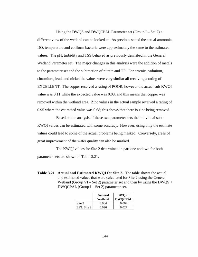
144

Using the DWQS and DWQCPAL Parameter set (Group I – Set 2) a

different view of the wetland can be looked at. As previous stated the actual ammonia,

DO, temperature and coliform bacteria were approximately the same to the estimated

values. The pH, turbidity and TSS behaved as previously described in the General

Wetland Parameter set. The major changes in this analysis were the addition of metals

to the parameter set and the subtraction of nitrate and TP. For arsenic, cadmium,

chromium, lead, and nickel the values were very similar all receiving a rating of

EXCELLENT. The copper received a rating of POOR, however the actual sub-KWQI

value was 0.11 while the expected value was 0.03, and this means that copper was

removed within the wetland area. Zinc values in the actual sample received a rating of

0.95 where the estimated value was 0.68; this shows that there is zinc being removed.

Based on the analysis of these two parameter sets the individual sub-

KWQI values can be estimated with some accuracy. However, using only the estimate

values could lead to some of the actual problems being masked. Conversely, areas of

great improvement of the water quality can also be masked.

The KWQI values for Site 2 determined in part one and two for both

parameter sets are shown in Table 3.21.

Table 3.21 Actual and Estimated KWQI for Site 2. The table shows the actual and estimated values that were calculated for Site 2 using the General Wetland (Group VI – Set 2) parameter set and then by using the DWQS + DWQCPAL (Group I – Set 2) parameter set.

General Wetland

DWQS + DWQCPAL

Site 2 0.004 0.004EST. Site 2 0.026 0.027

145

The values for the KWQI were significantly different than was expected

based on the values in the sub-KWQIs (Tables 3.19 and 3.20). The KWQI was

relatively the same regardless of the parameter set used; major differences occurred

between the actual values and the estimated values. These differences occurred

because of the differences in the lowest ranking sub-KWQI values. Since in the

aggregation process the lowest scoring values are favored to prevent masking of

impairment, the low scoring actual turbidity value had a significant affect on the total

KWQI value. In conclusion, the estimation can be used when no other data is

available but should not be relied on solely to provide accurate accounts of what is

occurring at Site 2 for the individual parameters or the total index rating.

Analysis of Riparian Buffer Zone between Sites 2 and 6

Riparian buffer zones are a very common BMP and once stabilized are

generally low maintenance. A riparian buffer zone lines the stream between Sites 2

and 6 as described previously. The analysis for the riparian buffer zone will be

completed using the Minimum (Group III-Set 1) and the General (Group III-Set 2)

riparian buffer parameter sets (Table 3.12). The two parameter sets were chosen to

show the difference between the calculated KWQI based on parameters affected by the

BMP and the calculated KWQI based on those BMP parameters as well as other

general stream health parameters. Calculations are based on yearly averages.

The sub-KWQI values calculated using the Minimum parameter set is

shown in Table 3.22 and the plot of the KWQI is shown in Figure 3.46. The low

KWQI values were caused by the excessive levels of TN, TP and TDS that were

present at both sites during the study (Table 3.19). Ammonia levels stayed the same

over the four years of the study maintaining a constant high sub-KWQI resulting in a

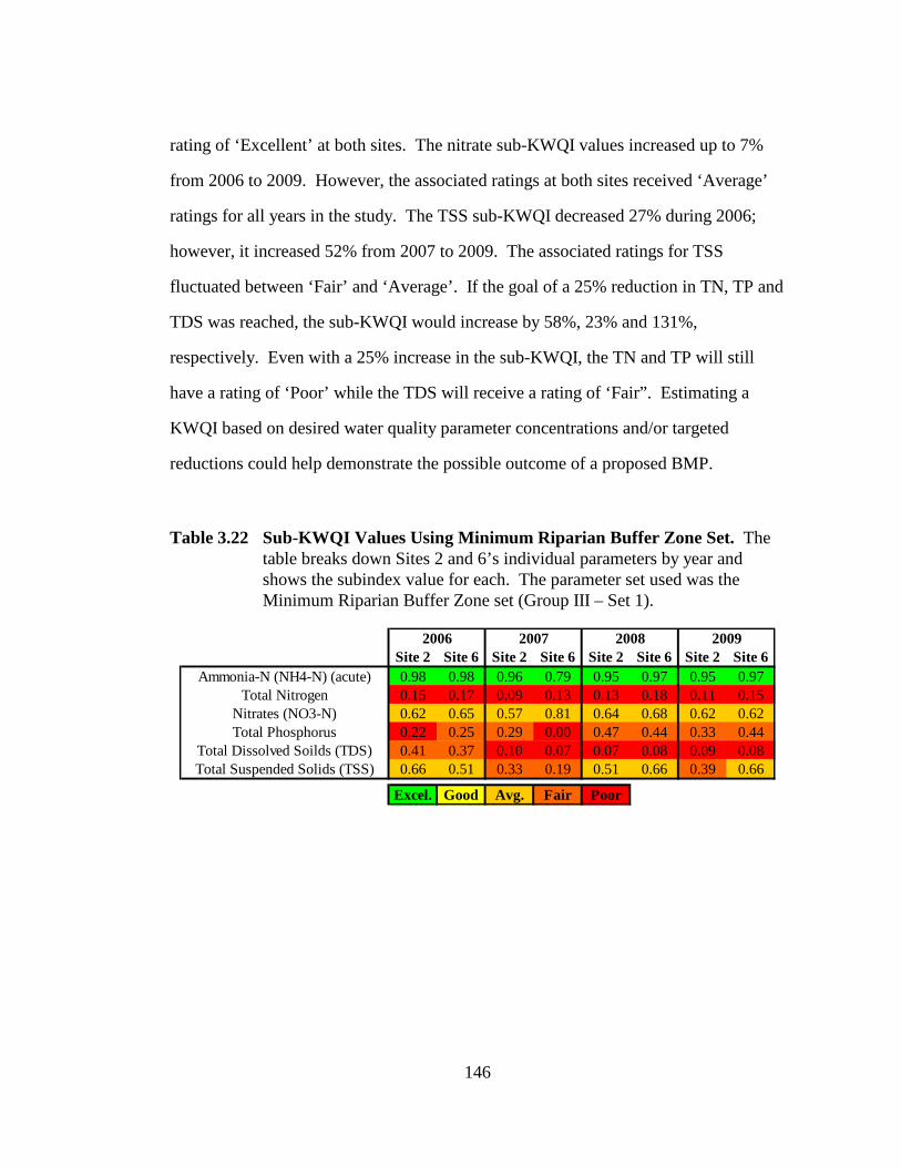
146

rating of ‘Excellent’ at both sites. The nitrate sub-KWQI values increased up to 7%

from 2006 to 2009. However, the associated ratings at both sites received ‘Average’

ratings for all years in the study. The TSS sub-KWQI decreased 27% during 2006;

however, it increased 52% from 2007 to 2009. The associated ratings for TSS

fluctuated between ‘Fair’ and ‘Average’. If the goal of a 25% reduction in TN, TP and

TDS was reached, the sub-KWQI would increase by 58%, 23% and 131%,

respectively. Even with a 25% increase in the sub-KWQI, the TN and TP will still

have a rating of ‘Poor’ while the TDS will receive a rating of ‘Fair”. Estimating a

KWQI based on desired water quality parameter concentrations and/or targeted

reductions could help demonstrate the possible outcome of a proposed BMP.

Table 3.22 Sub-KWQI Values Using Minimum Riparian Buffer Zone Set. The table breaks down Sites 2 and 6’s individual parameters by year and shows the subindex value for each. The parameter set used was the Minimum Riparian Buffer Zone set (Group III – Set 1).

Site 2 Site 6 Site 2 Site 6 Site 2 Site 6 Site 2 Site 6Ammonia-N (NH4-N) (acute) 0.98 0.98 0.96 0.79 0.95 0.97 0.95 0.97

Total Nitrogen 0.15 0.17 0.09 0.13 0.13 0.18 0.11 0.15Nitrates (NO3-N) 0.62 0.65 0.57 0.81 0.64 0.68 0.62 0.62Total Phosphorus 0.22 0.25 0.29 0.00 0.47 0.44 0.33 0.44

Total Dissolved Soilds (TDS) 0.41 0.37 0.10 0.07 0.07 0.08 0.09 0.08Total Suspended Solids (TSS) 0.66 0.51 0.33 0.19 0.51 0.66 0.39 0.66

Excel. Good Avg. Fair Poor

2006 2007 2008 2009

147

0.12

60

0.06

90

0.06

21

0.06

96

0.13

82

0.07

82

0.07

32

0.07

16

0.00

0.02

0.04

0.06

0.08

0.10

0.12

0.14

0.16

2006 2007 2008 2009

KW

QI V

alue

Site 2Site 6

Figure 3.46 KWQI Values Using Minimum Riparian Buffer Zone Set. This figure shows the KWQI values based on the yearly averages for Sites 2 and 6 using the Minimum Riparian Buffer Zone Set (Group III – Set 1).

The sub-KWQI values calculated using the General parameter set is

shown in Table 3.23 and the plot of the KWQI is shown in Figure 3.47. Site 6 KWQI

values decreased dramatically between the two parameter set assessments. This

decrease in KWQI values was due to the high concentration of chlorophyll a found

during all four years. Based on the first assessment, water quality between Site 2 and

Site 6 showed little to no improvement between 2007 and 2009 (Figure 3.46).

However, based on the larger parameter set assessment, the resulting KWQI values

show that the stream is more impaired after traveling through the riparian buffer zone

as it enters the pond area at Site 6 (Figure 3.47). This second set of parameters was

run to show that although the buffer zone can improve certain water quality

parameters, there are other problems that need to be addressed. Therefore, the system

should not be evaluated piecewise in terms of just the performance of BMPs;

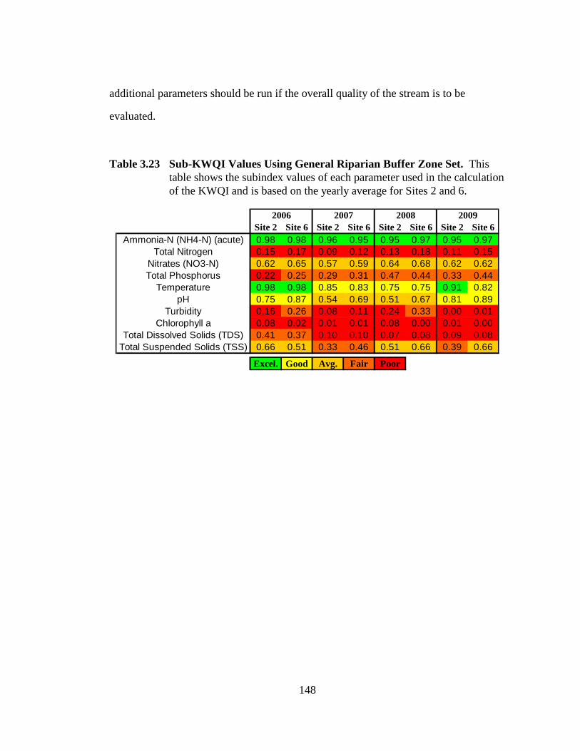
148

additional parameters should be run if the overall quality of the stream is to be

evaluated.

Table 3.23 Sub-KWQI Values Using General Riparian Buffer Zone Set. This table shows the subindex values of each parameter used in the calculation of the KWQI and is based on the yearly average for Sites 2 and 6.



Temperature 0.98 0.98 0.85 0.83 0.75 0.75 0.91 0.82pH 0.75 0.87 0.54 0.69 0.51 0.67 0.81 0.89

Turbidity 0.16 0.26 0.08 0.11 0.24 0.33 0.00 0.01Chlorophyll a 0.08 0.02 0.01 0.01 0.08 0.00 0.01 0.00

Total Dissolved Solids (TDS) 0.41 0.37 0.10 0.10 0.07 0.08 0.09 0.08Total Suspended Solids (TSS) 0.66 0.51 0.33 0.46 0.51 0.66 0.39 0.66


2006 2007 2008 2009

149

0.07

5

0.00

9

0.05

6

0.00

4

0.02

1

0.00

5

0.00

2

0.00

1

0.00

0.01

0.02

0.03

0.04

0.05

0.06

0.07

0.08

2006 2007 2008 2009

KW

QI V

alue

Site 2Site 6

Figure 3.47 KWQI Values Using General Riparian Buffer Zone Set. This figure shows the KWQI values based on the yearly averages for Sites 2 and 6 using the General Riparian Buffer Zone Set (Group III – Set 2)

There are some problems that occur between Sites 2 and 6 that were

noticed during stream exploration that may be affecting the calculated KWQI for Site

6. Site 6 has two culverts with the main channel flowing through the smaller of the

two culverts. This small culvert is almost fully clogged with debris on the other side

of Route 72 just upstream of the sampling location at Site 6. This is causing the

stream to cut though and erode a new path in the banks so the excess water and

associated sediments now flow through the larger storm culvert. If the blocked culvert

is cleared it will allow the stream to flow through the main channel with little soil

erosion and enter into Site 6 as a smooth flowing stream instead of a slow seep. This

will prevent ponding upstream of Site 6 where possible water quality impairment is

occurring. Another possible pollutant load entering the Cool Run upstream of Site 6 is

the surface runoff coming from the Newark Concrete Plant. The permitted discharge

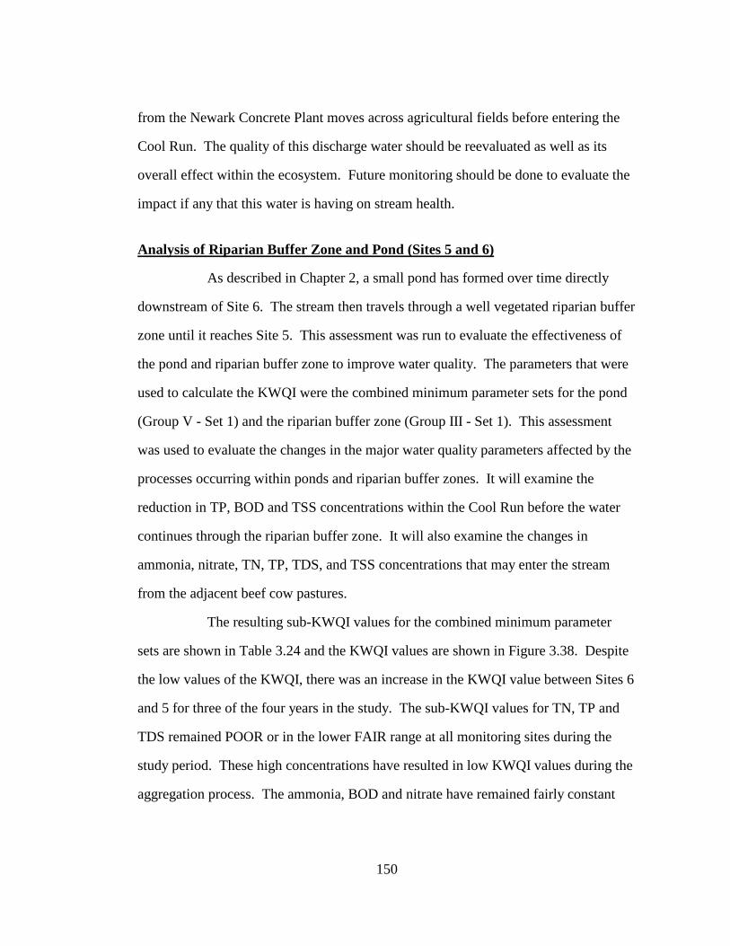
150

from the Newark Concrete Plant moves across agricultural fields before entering the

Cool Run. The quality of this discharge water should be reevaluated as well as its

overall effect within the ecosystem. Future monitoring should be done to evaluate the

impact if any that this water is having on stream health.

Analysis of Riparian Buffer Zone and Pond (Sites 5 and 6)

As described in Chapter 2, a small pond has formed over time directly

downstream of Site 6. The stream then travels through a well vegetated riparian buffer

zone until it reaches Site 5. This assessment was run to evaluate the effectiveness of

the pond and riparian buffer zone to improve water quality. The parameters that were

used to calculate the KWQI were the combined minimum parameter sets for the pond

(Group V - Set 1) and the riparian buffer zone (Group III - Set 1). This assessment

was used to evaluate the changes in the major water quality parameters affected by the

processes occurring within ponds and riparian buffer zones. It will examine the

reduction in TP, BOD and TSS concentrations within the Cool Run before the water

continues through the riparian buffer zone. It will also examine the changes in

ammonia, nitrate, TN, TP, TDS, and TSS concentrations that may enter the stream

from the adjacent beef cow pastures.

The resulting sub-KWQI values for the combined minimum parameter

sets are shown in Table 3.24 and the KWQI values are shown in Figure 3.38. Despite

the low values of the KWQI, there was an increase in the KWQI value between Sites 6

and 5 for three of the four years in the study. The sub-KWQI values for TN, TP and

TDS remained POOR or in the lower FAIR range at all monitoring sites during the

study period. These high concentrations have resulted in low KWQI values during the

aggregation process. The ammonia, BOD and nitrate have remained fairly constant

151

during the study period constantly received ratings of EXCELLENT, GOOD and

AVERAGE, respectively. The increase in KWQI values in 2008 and 2009 were the

result of the reduction in TSS.

Table 3.24 Sub-KWQI Values Using Minimum Riparian Buffer Zone and Pond Set. This table shows the subindex values of each parameter used in the calculation of the KWQI and is based on the yearly average for Sites 5 and 6.



BOD5 0.82 0.82 0.75 0.76 0.82 0.82 0.80 0.82Total Dissolved Soilds (TDS) 0.38 0.37 0.10 0.10 0.07 0.08 0.09 0.08Total Suspended Solids (TSS) 0.90 0.51 0.35 0.46 0.97 0.66 0.86 0.66


2006 2007 2008 2009

The low KWQI values indicate impairment in stream water quality due to

high concentrations of the parameters that the BMPs have been shown to reduce. This

type of analysis can help identify which water quality parameters are not improving

within a system influenced by the BMPs but will not provide information on the

general health of the stream. Modification of the parameter set used in the

assessments can be made to address particular concerns.

152

0.14

4

0.07

9

0.07

5

0.07

3

0.15

5

0.08

1

0.06

9

0.07

9

0.00

0.02

0.04

0.06

0.08

0.10

0.12

0.14

0.16

0.18

2006 2007 2008 2009

KW

QI V

alue

Site 6Site 5

Figure 3.48 KWQI Using Minimum Riparian Buffer Zone and Ponds/Basins Combined Parameter Sets. This figure shows the KWQI values based on the yearly averages for Sites 5 and 6 using the Minimum Riparian Buffer Zone Set (Group III – Set 1)

Analysis of Manure Collection System (Site 8)

Since the start of storm sample collection at Site 8 in 2007, there have

been a total of 15 storm flow samples collected. The yearly averages were used in the

calculation of the sub-KWQI values to determine if there have been improvements in

the quality of stormwater that runs through the fields and into the storm grate after

installation of the manure collection system. The Manure Collection Set (Group II-Set

2) was used to calculate the final KWQI values. The total number of samples collected

in 2007, 2008 and 2009 were 6, 8, and 1, respectively.

The sub-KWQI values for parameters included in the assessment are

shown in Figure 3.49.

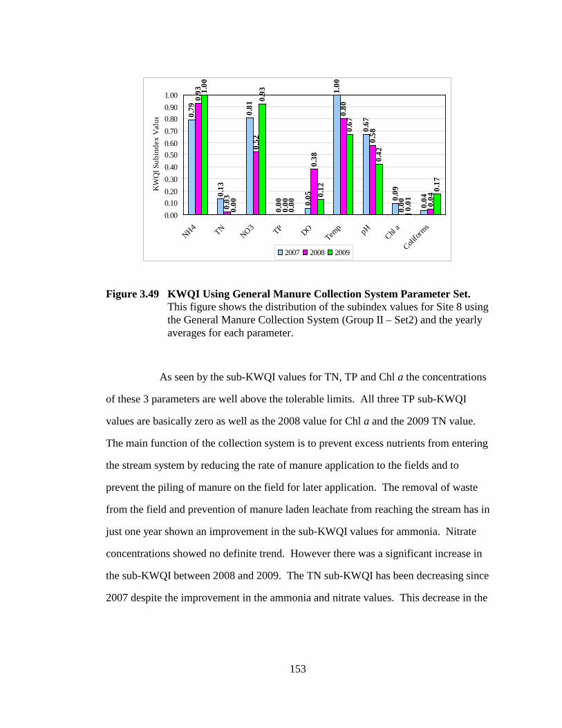
153

0.79

0.13

0.81

0.00 0.

05

1.00

0.67

0.09

0.04

0.93

0.03

0.52

0.00

0.38

0.80

0.58

0.00 0.

04

1.00

0.00

0.93

0.00

0.12

0.67

0.42

0.01

0.17

0.000.100.200.300.400.500.600.700.800.901.00

NH4 TNNO3 TP DO

Temp pH

Chl a

Colifor

ms

KW

QI S

ubin

dex

Val

ue

2007 2008 2009

Figure 3.49 KWQI Using General Manure Collection System Parameter Set. This figure shows the distribution of the subindex values for Site 8 using the General Manure Collection System (Group II – Set2) and the yearly averages for each parameter.

As seen by the sub-KWQI values for TN, TP and Chl a the concentrations

of these 3 parameters are well above the tolerable limits. All three TP sub-KWQI

values are basically zero as well as the 2008 value for Chl a and the 2009 TN value.

The main function of the collection system is to prevent excess nutrients from entering

the stream system by reducing the rate of manure application to the fields and to

prevent the piling of manure on the field for later application. The removal of waste

from the field and prevention of manure laden leachate from reaching the stream has in

just one year shown an improvement in the sub-KWQI values for ammonia. Nitrate

concentrations showed no definite trend. However there was a significant increase in

the sub-KWQI between 2008 and 2009. The TN sub-KWQI has been decreasing since

2007 despite the improvement in the ammonia and nitrate values. This decrease in the

154

TN sub-KWQI suggests that organic nitrogen is the main species of nitrogen present at

site 8. The DO sub-KWQI values have varied over the three years. This is suspected

to be the result of the outlet being clogged, grown over, and having very little water

movement. The most significant change can be seen in the coliform count resulting in

significant changes in the coliform sub-KWQI values. The improvement may not

seem that great based on the low sub-KWQI values. However, the colony forming

units (CFU) per 100 ml in 2007 was estimated to be 1.19 million. This was the year

the manure collection system was being installed. The first year the system was in

operation the CFU per 100 ml dropped to 596,740. The estimated values for 2009 are

3,600 CFU per 100 ml. This change in numbers represents a 1000 fold decrease in

coliform bacteria between 2007 and 2009. This is a significant change and if this trend

continues, the CFU per 100 ml for the site should reach the acceptable value of less

than 925 CFU per 100 ml as regulated by the state of Delaware. Temperature and pH

varied through the years. However, the sub-KWQI values were within the tolerable

ranges with ratings of “average” to “excellent”.

Some physical evidence can be seen were drainage problems still occur at

Site 8. During and after rain events the areas surrounding the storm grate flood and

will remain wet for weeks. A second major problem at this site occurs where the

stream opens up into a free flowing channel. The exit culvert is buried under

vegetation that has over grown the outlet and partially filled in the stream channel.

This is preventing the water from flowing freely from the site and continuing

downstream to Site 1.

155

Analysis of UD Farm (Standards and Criteria Approach)

Two approaches were used to analyze the total water quality of the Cool

Run within the NRECF. The first approach, the Standards and Criteria Approach

(SCA), uses a single set of parameters to evaluate the farm at each of the base flow

sites. The second method uses the general BMP parameter sets to determine the

KWQI based on changes in the water quality parameters most affected by the BMPs.

A major problem affecting the outcome of this assessment approach is the very low

KWQI values at most of the sites resulting in a rating of very poor. These low ratings

reduced the effectiveness of the spatial estimation plots. Another limitation that

occurred was that the individual sites could not be marked within the spatial plot.

Arrows and site numbers were added separately to illustrate the site locations because

of the difficulty in determining the individual peak at site locations.

The spatial estimation section of the model was used to create the plots

that are in Figure 3.50. Only 2006 plot does not include data from Sites 7 and 8,

monitoring for those sites started in 2007. Spatial plots were created using the

combined parameters in the DWQS, DWQCPAL, DWQCPHH and the USEPA

nutrient criteria (combined, known as Group 1 – Set 4) to determine the KWQI. In

order to show the differences in the sites the normal scale of 0 to 1 for the KWQI

values was decreased to 0 to 0.15 on all four of the plots. The peak of the elevation

plot is the path of the stream as it flows through the farm. Color changes indicate a

change in elevation range for the KWQI value. The values calculated using the KWQI

between 2006 and 2007 all decreased. This can be seen in the figure by the decreases

in the elevation of the peaks. In 2008, the quality of water coming from Site 4

decreased while the rest of the NRECF began to show an increase. You can see where

Site 1 starts to enter into the stream but at a much lower KWQI than those coming

156

from Sites 4 and 3. The spatial estimation tool can be more useful in the evaluation of

the farm when there have been significant improvements in the many parameters that

are impaired. For now the tool can show only a portion of the changes in water quality

of the Cool Run that is occurring within the NRECF.

157

a)

1S1

Relative LatitudeRelative Longitude

2006 Spatial Estimation

0.00-0.02 0.02-0.03 0.03-0.05 0.05-0.06 0.06-0.08 0.08-0.090.09-0.11 0.11-0.12 0.12-0.14 0.14-0.15

b)

1S1



0.00-0.02 0.02-0.03 0.03-0.05 0.05-0.06 0.06-0.08 0.08-0.090.09-0.11 0.11-0.12 0.12-0.14 0.14-0.15

Figure 3.50 Spatial Estimation Using DWQS + DWQCPAL + DWQCPHH + USEPA nutrient criteria – a) 2006 yearly averages, b) 2007 yearly averages.

4 3

2

6

5

1 8

7

7 8 1

4 3

2

5

6

158

c)

1S1



0.00-0.02 0.02-0.03 0.03-0.05 0.05-0.06 0.06-0.08 0.08-0.090.09-0.11 0.11-0.12 0.12-0.14 0.14-0.15

d)

1S1



0.00-0.02 0.02-0.03 0.03-0.05 0.05-0.06 0.06-0.08 0.08-0.090.09-0.11 0.11-0.12 0.12-0.14 0.14-0.15

Figure 3.50 cont. c) 2008 yearly averages, d) 2009 yearly averages

5

6

2

3

1 8

7

4

3

2

6

5

4

1 8

7

159

The distribution of coliform bacteria across the NRECF is shown in Figure

3.51. The most western monitoring station, Site 7, is located at the wetland exit. Both

the sub-KWQI values and the coliform bacteria concentrations at Site 7 indicated that

a significant decrease (94.5%) of the coliform bacteria occurred since 2007. Site 8,

located downstream of Site 7, had a 99.7% reduction in the coliform bacteria,

representing a thousand fold decrease in coliform numbers from 2007 to 2009. At Site

4, the coliform concentrations fluctuated over the four years of the study but had a

63.7% reduction in the coliform concentration. The sub-KWQI at Site 1 also

fluctuated during the study. Despite a fluctuation in concentration, coliform bacteria

decreased 22.7% from 2006 and 2009. Between 2006 and 2007, the greatest change in

the coliform bacteria sub-KWQI values occurred at Site 3. Further reductions in

coliform bacteria were recorded in 2008 and 2009. The overall reduction at Site 3

during this study period was 92.0%, which reduced the coliform concentration to the

State of Delaware’s target goal for instantaneous coliform count for secondary contact.

Water from Sites 1, 3 and 4 converge and flow into the stream at Site 2. The coliform

sub-KWQI at Site 2 increased every year representing a 91.9% reduction in coliform

concentration. This site also reached the State’s target criteria for instantaneous

measurements for secondary contact. The coliform sub-KWQI value at Site 6

fluctuated within 0.06 during the study period but there was an overall reduction of

34.7%. The lowest point on Cool Run that is sampled within the NRECF is located at

Site 5. Values for the coliform sub-KWQI at Site 5 increased during the study period

with a reduction of 89.5% in coliform concentration since 2006.

160

a)

b)

*M represents a million colonies/100mL

Figure 3.51 Spatial Coliform Distribution on UDAESF – a) West Side – Sites 1, 3, 4, 8 and 7 b) East Side – Sites 2, 5, and 6. The figure shows the KWQI and concentration (colonies/100mL) for each monitoring site for 2006, 2007, 2008 and 2009 respectively. (Image: Alison Kiliszek and bing.com)

KWQI Conc. - - 0.08 54767

KWQI Conc. - - 0.04 1.1M* 0.04 596740 0.17 3600

KWQI Conc. 0.13 10439 0.21 1872

KWQI Conc. 0.17 4144 0.14 7938 0.23 1259 0.22 1503

KWQI Conc. 0.13 10450 0.22 1510

KWQI Conc. 0.13 9772 0.17 4201 0.23 1318 0.24 1023

KWQI Conc. 0.21 1908 0.17 3899 0.21 1749 0.23 1245

KWQI Conc. 0.13 10077 0.16 5438

161

The distribution of dissolved oxygen (DO) concentrations across the

NRECF is shown in Figure 3.52. There was a 21.2% decrease in the DO concentration

at Site 7 since 2007 resulting in a continuous decrease in the DO sub-KWQI during the

study period. There was an increase of 28.3% in the overall DO concentration at Site

8, although DO concentration has fluctuated over the past three years. Neither Sites 7

nor 8 meet the State of Delaware’s DO minimum concentration. Despite the

fluctuation of DO concentration at Site 4 during the four year study, there was an

overall increase of 9.2% in the average DO concentration. Fluctuations of DO

concentrations and resulting sub-KQWI values during the study also occurred at Site 1.

Based on the DO concentrations measured from 2006 to 2009, a 31.2% reduction in

DO occurred. However, the 2009 DO concentrations did not meet the Delaware

standards. At Site 3, the DO concentrations showed some variations with a lower

average value occurring in 2008. However, during all the other years of the study, DO

concentrations met the required 4.0 mg/L for instantaneous grab sample value. At Site

2, the DO sub-KWQI ratings varied within the EXCELLENT range for 3 of the 4 years

of the study. Although a decrease of 4.0% in DO occurred since 2006, the 2009 sub-

KWQI values were still in the EXCELLENT range. At Site 6, the measured DO

concentrations fluctuated but never had yearly averages below the DE standard. The

DO concentration measured at this site increased by 5.0% during the study period.

Values for the sub-KWQI values at Site 5 decreased during the study period with a

reduction of 3.3% in DO concentration when compared to the 2006 values.

162

a)

b)

Figure 3.52 Spatial Dissolved Oxygen Distribution on UDAESF – a) West Side – Sites 1, 3, 4, 8 and 7 b) East Side – Sites 2, 5, and 6. The figure shows the KWQI and concentration (mg/L) for each monitoring site for 2006, 2007, 2008 and 2009 respectively. (Image: Alison Kiliszek and bing.com)

KWQI Conc. - - 0.43 4.82 0.42 4.78 0.21 3.80

KWQI Conc. - - 0.05 2.51 0.38 4.60 0.12 3.22

KWQI Conc. 0.11 3.11 0.10 3.00 0.01 1.58 0.03 2.14

KWQI Conc. 0.89 6.82 0.90 6.86 0.49 5.05 0.97 7.45

KWQI Conc. 0.99 8.87 1.00 8.26 0.63 5.59 1.00 8.65

KWQI Conc. 1.00 9.10 1.00 8.18 0.78 6.05 0.99 8.80

KWQI Conc. 0.98 7.96 1.00 8.41 0.74 6.23 1.00 8.36

KWQI Conc. 0.95 7.23 0.92 6.99 0.35 4.48 0.91 6.94

163

The distribution of Total Nitrogen (TN) concentrations across the NRECF

is shown in Figure 3.53. There was a 69.7% decrease in the TN concentration at Site 7

during the study. Yearly averages of TN concentrations decreased consistently since

2007 resulting in a consistent increase in the sub-KWQI. At Site 8, located down

stream of Site 7, there was a 4482% increase in the TN concentration. This extremely

high concentration was attributed to a single measurement that may have been an error

in the analysis. However, the flow at Site 8 has been problematic with ponding

occurring for days after a rain event. The concentration of TN at Site 4 fluctuated

during the study, but there was an overall increase of 11.2%. However, the TN

concentration at this site did not meet the target goal of 3 mg/L as an upper limit stated

in the 2008 Delaware 305(b) report. The TN sub-KWQI value at Site 1 fluctuated

during the study. The concentration of TN increased 61.2% from 2006 to 2009. The

TN concentration at this site also did not meet the State’s target level. The TN sub-

KWQI at Site 3 gradually increased between 2006 and 2009. The overall reduction in

TN during this study period was 13.2%. Total Nitrogen concentrations at Site 2

fluctuated, but had an overall increase of 19.4% in TN concentration. The TN sub-

KWQI at Site 6 varied by 0.06 during the study period, but there was an overall

increase in concentration of 9.4%. Values for the sub-KWQI values at Site 5, the

lowest monitoring station on Cool Run, decreased during the study period resulting in

an increase in TN of 5.2% since 2006. The TN concentrations at Sites 2, 6 and 5 do

not meet the DE standards for the targeted TN concentration goals.

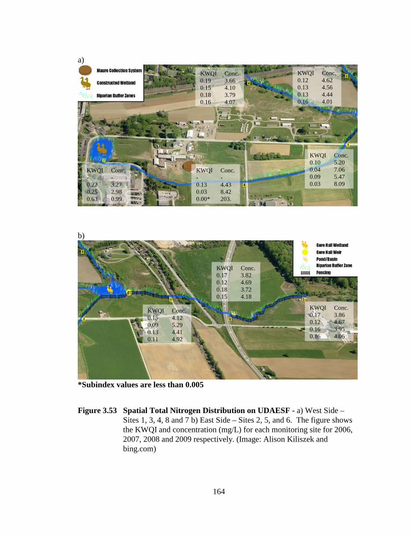
164

a)

b)

*Subindex values are less than 0.005

Figure 3.53 Spatial Total Nitrogen Distribution on UDAESF - a) West Side – Sites 1, 3, 4, 8 and 7 b) East Side – Sites 2, 5, and 6. The figure shows the KWQI and concentration (mg/L) for each monitoring site for 2006, 2007, 2008 and 2009 respectively. (Image: Alison Kiliszek and bing.com)

KWQI Conc. - - 0.22 3.27 0.25 2.98 0.63 0.99

KWQI Conc. - - 0.13 4.43 0.03 8.42 0.00* 203.

KWQI Conc. 0.10 5.20 0.04 7.06 0.09 5.47 0.03 8.09

KWQI Conc. 0.19 3.66 0.15 4.10 0.18 3.79 0.16 4.07

KWQI Conc. 0.12 4.62 0.13 4.56 0.13 4.44 0.16 4.01

KWQI Conc. 0.17 3.86 0.12 4.67 0.16 3.95 0.16 4.06

KWQI Conc. 0.17 3.82 0.12 4.69 0.18 3.72 0.15 4.18

KWQI Conc. 0.15 4.12 0.09 5.29 0.13 4.41 0.11 4.92

165

The distribution of Total Phosphorous (TP) concentrations across the

NREDF is shown in Figure 3.54. During the 2008 construction of the wetland, the

soils at the wetland outlet (Site 7) were disturbed coinciding with a significant peak in

the TP levels with resulting decreases in the sub-KWQI values. Despite the high

average TP concentration measured in 2008, there was a 46.7% reduction between

2007 and 2009. There was a 65% reduction in TP concentration at Site 8 during the

study. The sub-KWQI value at this site was reported as 0.00 because the high TP

concentration resulted in a sub-KWQI of less than 0.005. The TP concentration at Site

4 fluctuated during the study with a peak concentration in 2008. Despite the 2008

increase, the total reduction in TP between 2006 and 2009 was 50%. At Site 1, the TP

concentration also fluctuated during the study with similar sub-KWQI values as Site 8

(all values < 0.005). However, there was a 36.6% reduction in TP concentration

between 2006 and 2009. Since 2006, the TP concentration at Site 3 was reduced

64.7%. In 2009, the TP concentration at Site 3 was no longer above the 0.20 mg/L

target concentration of the 2008 Delaware 305(b) report. The TP sub-KWQI at Site 2

increased during the first three years of the study, with a slight decrease occurring in

2009. The yearly average TP concentration at Site 2 met the State’s upper

concentration target level since 2007. The sub-KWQI at Site 6 consistently increased

during the study period with a corresponding 40% reduction in TP. Although all the

TP concentration levels were in the upper range of the State’s target levels, the yearly

TP average at this site never exceeded the target value. Values for the sub-KWQI at

Site 5 have increased during the study period with a TP reduction of 25% from 2006 to

2009. Total P impairment of the Cool Run within the NRECF occurred but water

leaving Site 5 and the farm did not exceed the State’s upper level target concentration.

166

a)

b)


Figure 3.54 Spatial Total Phosphorus Distribution on UDAESF - a) West Side – Sites 1, 3, 4, 8 and 7 b) East Side – Sites 2, 5, and 6. The figure shows the KWQI and concentration (mg/L) for each monitoring site for 2006, 2007, 2008 and 2009 respectively. (Image: Alison Kiliszek and bing.com)

KWQI Conc. - - 0.13 0.30 0.01 0.62 0.33 0.16

KWQI Conc. - - 0.00* 2.83 0.00* 1.63 0.00* 0.99

KWQI Conc. 0.00* 2.02 0.00* 1.46 0.00* 1.93 0.00* 1.48

KWQI Conc. 0.66 0.06 0.62 0.07 0.07 0.38 0.81 0.03

KWQI Conc. 0.03 0.51 0.15 0.27 0.23 0.21 0.29 0.18

KWQI Conc. 0.33 0.16 0.29 0.18 0.57 0.08 0.44 0.12

KWQI Conc. 0.25 0.20 0.31 0.17 0.44 0.12 0.44 0.12

KWQI Conc. 0.22 0.22 0.29 0.18 0.47 0.11 0.33 0.16

167

The distribution of Total Suspended Solids (TSS) concentrations across

the NRECF is shown in Figure 3.55. There was a 100% reduction in TSS

concentration at Site 7 between 2007 and 2009. A low concentration of TSS is desired

within a water body which is why the sub-KWQI is not 1.00 at 0 mg/L TSS. At Site 8,

located down stream of Site 7, there was an 85.9% reduction in the TSS concentration.

The TSS concentrations at Site 4 fluctuated during the study but remained below 10

mg/L for the last three years of the study representing a total reduction of 46.2%. The

TSS concentrations at Site 1 doubled from 2006 to 2008 but returned to 2006 levels in

2009. There was a 333.3% increase in TSS concentration at Site 3 during the study

resulting in a drop in the sub-KWQI rating from EXCELLENT to FAIR. There was a

73.3% increase in TSS at Site 2, but the sub-KWQI value remained in the FAIR range.

However, there has been a visible increase in deposited sediments at the site over the

course of the study. The TSS concentration at Site 6 slowly but consistently decreased

during the study period with an overall 25% reduction. Values for the TSS sub-KWQI

at Site 5 increased during the second year of the study then decreased during the third

year of the study resulting in an 11.1% increase. Despite the increase, the rating

remained in the upper GOOD range of the sub-KWQI.

The use of the total KWQI value is to aid in a general assessment of water

quality in the area. It is also a tool that can easily determine if a stream is impaired in

some way. The additional use of the subindices can identify which water quality

parameters have the greatest impact on stream health. Examining the changes in the

individual water quality parameters and their associated sub-KWQI values over time

can provide a more detailed description of the effects of BMP implementation in a

watershed.

168

a)

b)


Figure 3.55 Spatial Total Suspended Solids Distribution on UDAESF - a) West Side – Sites 1, 4, 8 and 7 b) East Side – Sites 1, 2, 3, 5, and 6. The figure shows the KWQI and concentration (mg/L) for each monitoring site for 2006, 2007, 2008 and 2009 respectively. (Image: Alison Kiliszek and bing.com)

KWQI Conc. - - 0.08 113 0.21 46 0.75 0

KWQI Conc. - - 0.19 49 0.13 71 0.91 2

KWQI Conc. 0.30 33 0.14 64 0.14 66 0.32 31

KWQI Conc. 0.73 13 0.99 6 1.00 5 0.97 7

KWQI Conc. 0.99 6 0.99 6 0.66 15 0.39 26

KWQI Conc. 0.90 9 0.35 29 0.99 7 0.86 10

KWQI Conc. 0.51 20 0.46 22 0.66 15 0.66 15

KWQI Conc. 0.66 15 0.33 30 0.51 20 0.39 26

169

Analysis of UD Farm (BMP Approach)

This analysis approach involved using a variable set of parameters per site

to calculate the KWQI. This option is not available in the final version of the model.

Using a mixture of the BMP parameter sets, allowed for each site to be rated on the

parameters most affected by the BMPs. This method is to be used for the evaluation

of the BMPs within the farm with some general water quality health standards mixed

in. The analysis was only preformed on Sites 1 through 6. Site 1 KWQI was

calculated using the general manure collection system parameters (Group II - Set 2).

Site 2 KWQI was calculated using a combination of the general wetland and riparian

buffer zone parameter sets (Group IV - Set 2 and Group III - Set 2). The KWQIs for

Sites 3, 4 and 6 were all calculated using the general riparian buffer zone set (Group III

- Set 2). Site 5 KWQI was calculated using the general riparian buffer zone (Group III

- Set 2) and the pond/basins sets (Group V - Set 2).

The spatial plots of the calculated KWQI for the four years of the study are

shown in Figure 3.56. Again, they represent the change in the KWQI of the Cool Run

as it moves through the NRCF. From 2006 to 2007, there seems to be a general

decrease in the KWQI values over the whole farm. In 2008, the KWQI increases at

certain sections of the Cool Run indicating improvement in stream health at those

locations. Improvements can be seen near the location of the Gore Hall Wetland and

the riparian buffer zone that follows the stream after the pond/basin at Site 6. The

2009 spatial estimation shows a general decline in the water quality as it approaches

Site 6. However after passing this site the KWQI increases slightly. The parts of the

stream can be seen in the 2009 Spatial Estimation plot in Figure 3.56 illustrating that

although the stream is impaired, there has been an improvement in the quality of water

that is leaving the farm.

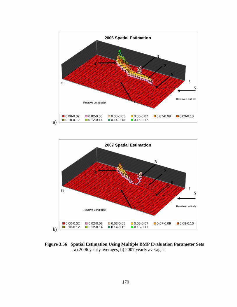
170

a)

1S1



0.00-0.02 0.02-0.03 0.03-0.05 0.05-0.07 0.07-0.09 0.09-0.100.10-0.12 0.12-0.14 0.14-0.15 0.15-0.17

b)

1S1



0.00-0.02 0.02-0.03 0.03-0.05 0.05-0.07 0.07-0.09 0.09-0.100.10-0.12 0.12-0.14 0.14-0.15 0.15-0.17

Figure 3.56 Spatial Estimation Using Multiple BMP Evaluation Parameter Sets – a) 2006 yearly averages, b) 2007 yearly averages

1

2

3 4

5

6

5

1

4

3

2

6

171

c)

1S1



0.00-0.02 0.02-0.03 0.03-0.05 0.05-0.07 0.07-0.09 0.09-0.100.10-0.12 0.12-0.14 0.14-0.15 0.15-0.17

d)

1S1



0.00-0.02 0.02-0.03 0.03-0.05 0.05-0.07 0.07-0.09 0.09-0.100.10-0.12 0.12-0.14 0.14-0.15 0.15-0.17

Figure 3.56 cont. – c) 2008 yearly averages, 2009 yearly averages

3

2

2

6

1

4

5

5

6

2 3

1

4

172

CHAPTER 4

CONCLUSIONS AND FUTURE GOALS

There are many conclusions that can be drawn from this project. One of

the objectives of the project was to answer the question “Are the BMPs helping to

improve the quality of water within the UDEW?” The answer to this question is yes.

The BMPs are having a positive impact on the watershed when looking at the whole

picture. The monitoring time table for this project is too short of a period to make

long term analyses of the BMPs and their effects on the water quality of the Cool Run

as it leaves the NRECF. The BMPs implemented during the course of the project now

have a basis for future evaluation. As discussed previously, many of the ecosystem

processes involved in pollutant removal take a significant amount of time.

Improvements in the watershed may not become evident for years. However,

assessments using the KWQI Model can help identify small changes that may occur in

relatively short time periods. A main goal for the future is to improve the health of the

Cool Run stream throughout the NRECF so that it is not impaired as it enters into the

Christina River. Setting smaller goals at certain key points along the stream where

there is the most impairment will hopefully have the greatest impact on the

downstream regions of Cool Run. For instance, repairing the riparian buffer zone

between Sites 8 and 1 and then from Site 1 until the Gore Hall Wetland should greatly

reduce the amount of nutrients and solids entering the stream. Improving water quality

in the upper reaches of the Cool Run on the NRECF should improve downstream

water quality and eventually increase the KWQI value at Site 5 as the water leaves the

173

area. Setting a reasonable goal to be reached within 5 years will allow the riparian

buffer zone to stabilize from the initial reconstruction.

One of the changes that should be made to the pasture and crop land

would be to install better drainage systems. There are many fields that have large

areas that do not drain becoming deposition areas that then get flushed during the next

storm event. These flushing events could cause abnormal spikes in the concentrations

of the parameters being measured. The dairy cow pasture near Site 8 and the beef cow

pasture area adjacent to Site 5 should be the first two sections worked on. These areas

flood every storm event and take up to a few weeks to dry out naturally.

The final future goal is to reduce the overall cost of the monitoring project

by decreasing sample events while still maintaining a good representation of data for

each of the parameters. To achieve this, a simple statistical analysis was performed on

the last twelve data points for each of the parameters for Sites 1 through 6 to determine

the minimum number of sample events required. Using the average of the values, a

standard deviation and confidence interval was determined. The confidence interval

was set at 95% for this analysis. The goal was to determine the minimum number of

samples that could be taken and still have an average between the upper and lower

limit of the confidence interval for all six sites. Using this method the parameters

ranged from being taken once a year to 6 times a year. The parameters that should be

taken every other month are coliform bacteria, copper, total nitrogen and nitrate.

Parameters that should be taken 5 times during the year are chlorophyll a, nickel,

chromium, cadmium and ammonia. Samples should be analyzed for total suspended

solids, dissolved oxygen, lead, arsenic, and total phosphorus at least once every three

months. The zinc can be monitored quarterly. Turbidity should be measured once

174

every six months. Parameters such as total dissolved solids, conductivity, pH,

temperature, BOD, and boron only need to be monitored once a year to be within the

estimated confidence interval.

Storm samples from Sites 7 and 8 should still be monitored quarterly or

after a storm event lasting an extended amount of time or after a large storm event.

Extended storm events would include rain that falls over a period of more than 8 hours

or events that last a series of days. Large storm events would include events that are

expected to have 2-4 inches or more of rain within a 24 hour period or shorter.

Samples should be collected within 72 hours after the end of the storm event. Storm

flow samples from Sites 1 through 8 should be collected at least twice a year so that an

analysis of storm event pollutant loading can be calculated and compared to base flow

situations.

175

REFERENCES

Biswas, Asit K., 1997. “Water Resources: Environmental Planning, Management, and Development”. McGraw-Hill Inc. Washington, D.C.

Bryant, Curtis W., 1987. “Lagoons, Ponds, and Aerobic Digestion”. Journal of Water Pollution Control Federation 59(6): 401-403.

Campagnini, J. and Kauffman, G., 2001. “Development of the University of Delaware Experimental Watershed Project”. University of Delaware, Pp. 1-31.

Carruthers, T. and C. Wazniak, 2004. “Development of a water quality index for the Maryland coastal bays.” Maryland’s Coastal Bays: Ecosystem Health Assessment, Chapter 4.4. pp. 4-59—4-65. Maryland Department of Natural Resources, Annapolis, Maryland. http://www.dnr.state.md.us/coastalbays/sob_2004.html. Accessed September 8, 2008.

Clesceri, L. S., Greenberg, A. E., Trussell, R. R. (Eds), 1989. “Standard Methods for the Examination of Water and Wastewater”. 17th ed., American Public Health Association, American Water Works Association and Water Pollution Control Federation, Washington, D.C., pp.4-75-4-81.

Coles-Ritchie, M. C., D. W. Roberts, J. L. Kershner, and R. C. Henderson. 2007. “Use of a wetland index to evaluate changes in riparian vegetation after livestock exclusion.” Journal of the American Water Resources Association (JAWRA) 43:731-743.

Corbitt, Robert A. 1990. “Standard Handbook of Environmental Engineering.” Mc Grawl-Hill Inc. Washington, D.C.

176

Cude, C. G. 2001. “Oregon water quality index: tool for evaluating water quality management effectiveness.” Journal of the American Water Resources Association 37(1): 125-137.

Delaware River Basin Commission, 2009. “Basin Facts.” <http://www.state.nj.us/drbc/thedrb.htm>. September 14, 2009.

DNREC, 2004. “State Of Delaware Surface Water Quality Standards As Amended, July 11, 2004.” Department of Natural Resources and Control. Dover, Delaware. pp 46.

DNREC, 2008. “State of Delaware 2008 Combined Watershed Assessment Report (305(b)) and Determination for the Clean Water Act Section 303(d) List of Waters Needing TMDLs.” Department of Natural Resources and Control. Dover, Delaware. pp 204.

Edwards, C. L., R. D. Shannon and A. R. Jarrett, 1999. “Sedimentation Basin Retention Efficiencies for Sediment, Nitrogen, and Phosphorus from Simulated Agricultural Runoff”. American Society of Agricultural and Biological Engineers 42(2): 403-409.

Emerson, Clay H., Claire Welty, and Robert G. Traver, 2005. “Watershed-Scale Evaluation of a System of Storm Water Detention Basins”. Journal of Hydrologic Engineering 10(3): 237-242.

Environmental Laboratory. 1987. Corps of Engineers wetlands delineation manual. US Army Engineer Waterways experiment Station. Vicksburg, MS, USA. Technical Report Y-87-1.

177

Gupta, A. K., Gupta, S. K. and Patil, Rashmi S.(2003) 'A Comparison of Water Quality Indices for Coastal Water', Journal of Environmental Science and Health, Part A, 38 (11): 2711-2725

Harrell, Tara. 2002. “Linking Stream Health and Land Use in the University of Delaware Experimental Watershed.” University of Delaware Senior Thesis.

House, M. A. 1990. “Water quality indices as indicators of ecosystem change.” Environmental Monitoring and Assessment 15: 255-263.

Kaurish, F. W. and T. Younos. 2007. “Developing a standardized water quality index for evaluating surface water quality.” Journal of the American Water Resources Association 43(2): 533-545.

Kovacic, David A., Mark B. David and Lowell E. Gentry, 2000. “Effectiveness of constructed wetlands in reducing nitrogen and phosphorus from agricultural tile drainage”. Journal of Environmental Quality 29(4):1264-1274.

Line, D. E., W. A. Harman, G. D. Jennings, E. J. Thompson, and D. L. Osmond, 2000. “Nonpoint-Source Pollutant Load Reductions Associated with Livestock Exclusion”. Journal of Environmental Quality. 29(6):1882-1890.

Maret, T. R., D. E. MacCoy, and D. M. Carlisle, 2008. “Long-Term Water Quality and Biological Responses to Multiple Best Management Practices in Rock Creek, Idaho”. Journal of the American Water Resources Association (JAWRA) 44(5):1248-1269

McDermott, Jenny. 2009. Email correspondence on BMPs

178

McDermott, J and J.T. Sims. 2007. Request for Funding to Monitor Cool Run Surface Water at the College of Agriculture and Natural Resources, University of Delaware (UD-CANR). Prepared November 14, 2005.

Meals, Donald W., Steven A. Dressing, and Thomas E. Davenport, 2010. “Lag Time in Water Quality Response to Best Management Practices: A Review”. Journal of Environmental Quality. 39:85-96.

Meindl, Christopher F., (2005). “Wetland Diversity: The Limits of Generalization”. Journal of Geography 104(6): 243-256

Meyer, D. Morse, I. Garnett, and J. C. Guthrie, 1997. “A Survey of Dairy Manure Management Practices in California”. Journal of Dairy Science 80:1841-1845.

Ott, W.R., 1978. Environmental Indices. Theory and Practice. Ann Arbor science. Washington, D.C.

Pesce, S. and D.A. Wunderlin. 2000. “Use of water quality indices to verify the impact of Córdoba City (Argintina) on Suquía River.” Water Research 34(11): 2915-2926.

Phillips, Jonathan D., 1990. “Fluvial Sediment Storage in Wetlands”. Journal of the American Water Resources Association. 25(4):867-873.

Powell, J. Mark, Daniel F. McCrory, and D. B. Jackson-Smith, and H. Saam, 2005. “Manure Collection and Distribution on Wisconsin Dairy Farms”. Journal of Environmental Quality. 34(6):2036-2044.

179

Reinhardt, Miriam, Beat Müller, René Gächter and Bernhard Wehrl. 2006. “Nitrogen Removal in a Small Constructed Wetland: An Isotope Mass Balance Approach.” Environmental Science and Technology 40(10): 3310-3319.

Schoeneberger, P.J., D.A. Wysocki, D.A. Benham, and W.D. Broderson. 2002. Field book for describing and sampling soils. Ver. 2.0. Natural resources Conservation Service, National Soil Survey Center, Lincoln, NE, USA.

Sims, J.T. and J. McDermott, 2008. Best Management Practices to Improve Water Quality in an Impaired Tributary and as an Educational Resource for the Environmental Sustainability Initiative at the University of Delaware. Proposal for Delaware Department of Natural Resources and Environmental Control. CWA 319 Funding pp 1-8.

Strahler, Arthur N. “Geology Part II.” Handbook of Applied Hydrology. Ed. Ven Te Chow. Vol. 8. New York: McGraw Hill Book Company, 1964. 39 – 76.

Swamee, P. K. and A. Tyagi. 2000. “Describing Water Quality with Aggregate Index.” Journal of Environmental Engineering 126(5): 451- 455.

Swamee, P. K. and A. Tyagi. 2007. “Improved method for aggregation of water quality subindices.” Journal of Environmental Engineering 133(2): 220-225.

Tabacchi, Eric, Luc Lambs, Helene Guilloy, Anne-Marie Planty-Tabacchi, Etienne Muller, and Henri Decamps, 2000. “Impacts of riparian vegetation on hydrological processes”. Hydrological Processes 14: 2959-2976.

Todd, Albert H. 2008. “Riparian Ecosystems and Buffers: Working at the Water’s Edge.” Water Resources IMPACT 10(3):3-5.

180

US EPA, 1987. “Quality Criteria for Water 1986 [The Gold Book].” Rep. 440/5-86-001. USEPA Office Of Water Regulations and Standards, Washington, DC.

US EPA, 2000. “Ambient Water Quality Criteria Recommendations.” Rep. 822-B-00-022. USEPA Office of Water (4304), 1200 Pennsylvania Avenue, NW, Washington, DC.

US EPA. 2006. “Volunteer Stream Monitoring: A Methods Manual.” USEPA Rep. 841-B-97-003. USEPA Office of Water (4503F), 1200 Pennsylvania Avenue, NW, Washington, DC.

US EPA, 2008. “EPA Region 7 4B Rationale.” <http://www.epa.gov/region7/water/pdf/upper_delaware_river_cedar_creek_review.pdf>.

US EPA, Water Quality Criteria. “Ecoregional Criteria: Summary Table for the Nutrient Criteria Documents.” <http://www.epa.gov/waterscience/criteria/nutrient/ecoregions/files/sumtable.pdf>. October 22, 2009.

USDA, NRCS. 2002. Field indicators of hydric soils in the United States, Version 5.0. G.W. Hurt, P.M. Whited, and R.F. Pringle (eds.). USDA, NRCS in cooperation with the National Technical Committee for Hydric Soils, Fort Worth, TX

Varadharajan, Raman D., Reinier Bouweester and Mohan S. 2009 “Fuzzy Logic Water Quality Index and Importance of Water Quality Parameters” Air, Soil and Water Research 2:51-59

181

Vidon, Phillippe, Craig Allan, and Richard Lowrance. 2008. “Generalizing Riparian Zone Function at the Landscape Scale.” Water Resources IMPCAT 10(3): 12-14

Watershed Professionals Network, 1999. “Oregon Watershed Assessment Manual” June 1999. Prepared for the Governor’s Watershed Enhancement Board. Salem, Oregon.