development of a novel air hybrid engine
TRANSCRIPT
Development of a Novel Air Hybrid
Engine
by
Amir Fazeli
A thesis
presented to the University of Waterloo
in fulfillment of the
thesis requirement for the degree of
PhD
in
Mechanical and Mechatronics Engineering
Waterloo, Ontario, Canada, 2011
©Amir Fazeli 2011

ii
AUTHOR'S DECLARATION
I hereby declare that I am the sole author of this thesis. This is a true copy of the thesis, including any
required final revisions, as accepted by my examiners.
I understand that my thesis may be made electronically available to the public.
iii
Abstract
An air hybrid vehicle is an alternative to the electric hybrid vehicle that stores the kinetic
energy of the vehicle during braking in the form of pressurized air. In this thesis, a novel
compression strategy for an air hybrid engine is developed that increases the efficiency of
conventional air hybrid engines significantly. The new air hybrid engine utilizes a new
compression process in which two air tanks are used to increase the air pressure during the
engine compressor mode. To develop the new engine, its mathematical model is derived and
validated using GT-Power software. An experimental setup has also been designed to test the
performance of the proposed system. The experimental results show the superiority of the
new configuration over conventional single-tank system in storing energy.
In addition, a new switchable cam-based valvetrain and cylinder head is proposed to
eliminate the need for a fully flexible valve system in air hybrid engines. The cam-based
valvetrain can be used both for the conventional and the proposed double-tank air hybrid
engines. To control the engine braking torque using this valvetrain, the same throttle that
controls the traction torque is used. Model-based and model-free control methods are adopted
to develop a controller for the engine braking torque. The new throttle-based air hybrid
engine torque control is modeled and validated by simulation and experiments. The fuel
economy obtained in a drive cycle by a double-tank air hybrid vehicle is evaluated and
compared to that of a single-tank air hybrid vehicle.

iv
Acknowledgments
I would like to express my deepest gratitude to my supervisors Professor Amir Khajepour
and Professor Cécile Devaud for their guidance and continuous support throughout my
graduate studies at University of Waterloo. I cannot thank them enough for all they have
done for me.
I am also grateful to my committee members, Prof. Roydon Fraser, Prof. Bill Epling, Prof.
Behrad Khamesee and Prof. Lino Guzzella, for their insightful comments and valuable
suggestions.
I am grateful for Mahsa, my beloved wife, for her patience and support. She stood by me
through all the successes and setbacks during the last four years. I want to thank my parents,
Maryam Ghavidel Tehrani and Mohammad Javad Fazeli for their unconditional support and
continuous encouragement. I also wish to thank my sisters, Torfeh and Elham Fazeli for their
love and support.
My special thanks to all my friends who helped me over the years: Ali Nabi, Mohammad
Pournazeri, Dr. Hamid Bolandhemmat, Negar Rasti, Dr. Meisam Amiri, Omid Aminfar,
Soroosh Hassanpour, Dr. Vahid Fallah, Dr. Meysar Zeinali, Dr. Nasser Lashgarian and
Saman Mohammadi.
I would like to thank all the staff at the University of Waterloo who gave me this
opportunity to learn and grow.
The financial support from Ontario Centres of Excellence (OCE) and Natural Sciences and
Engineering Research Council of Canada (NSERC) is also appreciated.
v
Table of Contents AUTHOR'S DECLARATION ............................................................................................................... ii
Abstract ................................................................................................................................................. iii
Acknowledgments ................................................................................................................................. iv
Table of Contents ................................................................................................................................... v
List of Figures ..................................................................................................................................... viii
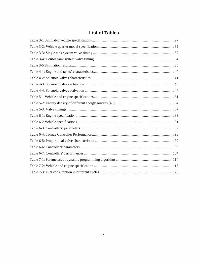
List of Tables ......................................................................................................................................... xi
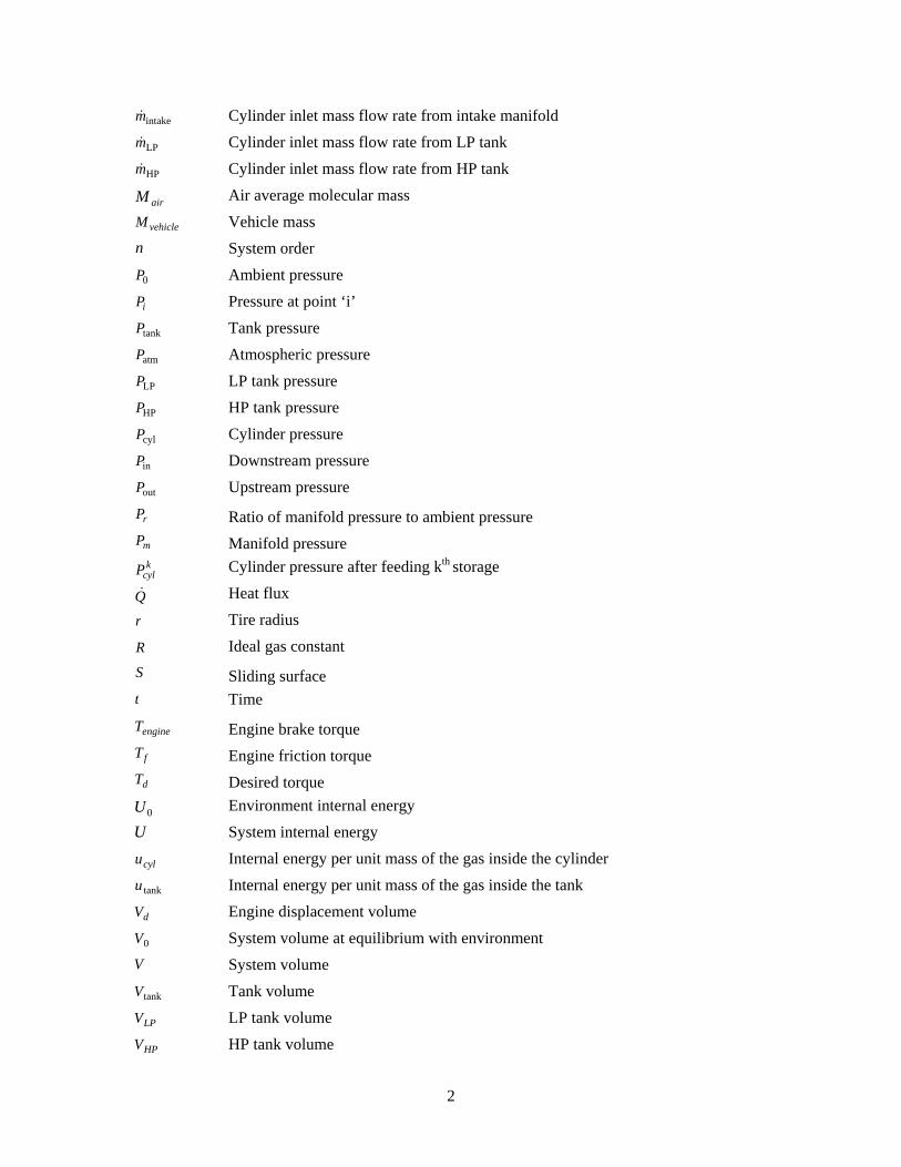
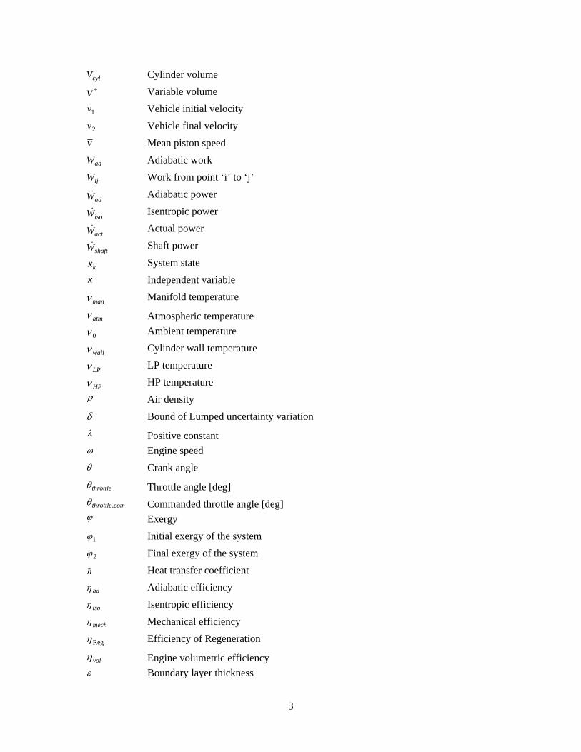
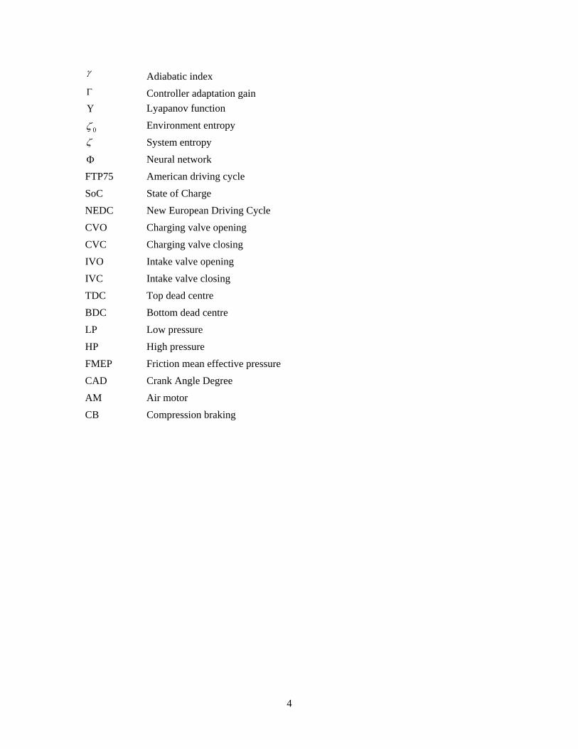
Nomenclature ......................................................................................................................................... 1
Chapter 1 Introduction ............................................................................................................................ 5
1.1 Air Hybrid Vehicles ..................................................................................................................... 5
1.2 Implementation of Air Hybrid Engines ........................................................................................ 8
1.3 Research Objectives and Thesis Layout ....................................................................................... 9
Chapter 2 Literature Review ................................................................................................................ 11
2.1 Air Hybrid Vehicles ................................................................................................................... 11
2.1.1 UCLA Research Group ....................................................................................................... 13
2.1.2 Lund Institute of Technology .............................................................................................. 14
2.1.3 Brunel University ................................................................................................................ 15
2.1.4 Institute PRISME/ EMP Université d’Orléans .................................................................... 16
2.1.5 ETH University ................................................................................................................... 16
2.1.6 National Taipei University of Technology .......................................................................... 17
2.2 Summary .................................................................................................................................... 17
Chapter 3 Double-tank Compression Strategy ..................................................................................... 18
3.1 Efficiency of Energy Storing ...................................................................................................... 18
3.2 Single-tank (conventional) Regenerative Braking ..................................................................... 19
3.3 Double-tank Regenerative Braking ............................................................................................ 23
3.4 Simulations ................................................................................................................................. 27
3.5 Detailed System Modeling Based on the First Law of Thermodynamics .................................. 28
3.6 Simulation of Mathematical and GT-POWER Models .............................................................. 32
3.7 Summary .................................................................................................................................... 37
Chapter 4 Experimental Analysis ......................................................................................................... 38
4.1 Test Procedure ............................................................................................................................ 42
4.2 Experimental Results .................................................................................................................. 43
vi
4.3 Summary .................................................................................................................................... 47
Chapter 5 Cam-based Air Hybrid Engine ............................................................................................ 48
5.1 Background ................................................................................................................................ 48
5.2 Cam-based Valvetrain ................................................................................................................ 50
5.3 Cam-based Single-tank Configuration ....................................................................................... 52
5.4 Cam-based Double-tank Configuration ..................................................................................... 55
5.5 Pros and Cons of the Proposed Air Hybrid Configuration ........................................................ 59
5.6 Simulations ................................................................................................................................ 60
5.6.1 Regenerative Braking .......................................................................................................... 60
5.6.2 Air Motor Mode .................................................................................................................. 63
5.7 Experimental Studies ................................................................................................................. 66
5.7.1 Regenerative Braking Mode ............................................................................................... 68
5.7.2 Air Motor Mode .................................................................................................................. 74
5.8 Summary .................................................................................................................................... 76
Chapter 6 Regenerative Braking Torque Control ................................................................................ 78
6.1 Background ................................................................................................................................ 78
6.2 Regenerative Braking Mean Value Model (MVM) ................................................................... 79
6.3 Robust Regenerative Torque Controller Design ........................................................................ 85
6.3.1 Controller Design for Nominal System .............................................................................. 86
6.3.2 Controller Design for System with Uncertainty .................................................................. 88
6.3.3 Stability and Robustness Analysis ...................................................................................... 88
6.4 Simulation and Numerical Results ............................................................................................. 91
6.5 Experiments ............................................................................................................................... 98
6.5.1 Experimental Procedure ...................................................................................................... 98
6.5.2 Single-tank Regenerative Torque Control .......................................................................... 99
6.5.3 Double-tank Regenerative Torque Control ....................................................................... 105
6.6 Summary .................................................................................................................................. 110
Chapter 7 Drive Cycle Simulations ................................................................................................... 111
7.1 Background .............................................................................................................................. 111
7.1.1 Dynamic Programming ..................................................................................................... 111
7.1.2 Application of Dynamic Programming ............................................................................. 113
7.2 Implementation of the Dynamic Programming ........................................................................ 114
vii
7.2.1 UDDS Drive Cycle ............................................................................................................ 120
7.2.2 FTP75 Drive Cycle ............................................................................................................ 123
7.3 Optimum Fuel Consumption .................................................................................................... 126
7.4 Summary .................................................................................................................................. 126
Chapter 8 Conclusions and Future Work ........................................................................................... 128
8.1 Summary of Contributions ....................................................................................................... 128
8.2 Publications Resulted from This Thesis ................................................................................... 129
8.3 Suggestions for Future Work .................................................................................................... 130
Appendix A ........................................................................................................................................ 131
Compressor Efficiency Definitions .................................................................................................... 131
Appendix B ......................................................................................................................................... 134
Regenerative Braking Thermodynamic Cycle ................................................................................... 134
Appendix C ......................................................................................................................................... 137
LP tank capacity ................................................................................................................................. 137
Appendix D ........................................................................................................................................ 140
Multi-tank Compression ..................................................................................................................... 140
Appendix E Simulation Parameters .................................................................................................... 143
Appendix F ......................................................................................................................................... 144
Voltage to Current Converter Drive ................................................................................................... 144
Appendix G Voltage to Current Converter Drive .............................................................................. 147
Appendix H Identifying the Engine Dynamic Model ........................................................................ 148
Appendix I Accessory assisting Mode ............................................................................................... 151
Reference ............................................................................................................................................ 153
viii
List of Figures Figure 1-1: Energy flow in the CB mode ............................................................................................... 5
Figure 1-2: Energy flow in the AM mode .............................................................................................. 6
Figure 1-3: Series configuration for running the engine accessories ..................................................... 7
Figure 1-4: Parallel configuration for running the engine accessories ................................................... 7
Figure 1-5: Energy flow in supercharged mode ..................................................................................... 8
Figure 2-1: Schechter’s proposed configuration [12] .......................................................................... 12
Figure 2-2: Air hybrid concept using two tanks [18] ........................................................................... 14
Figure 3-1: Regenerative braking ideal air cycle ................................................................................. 20
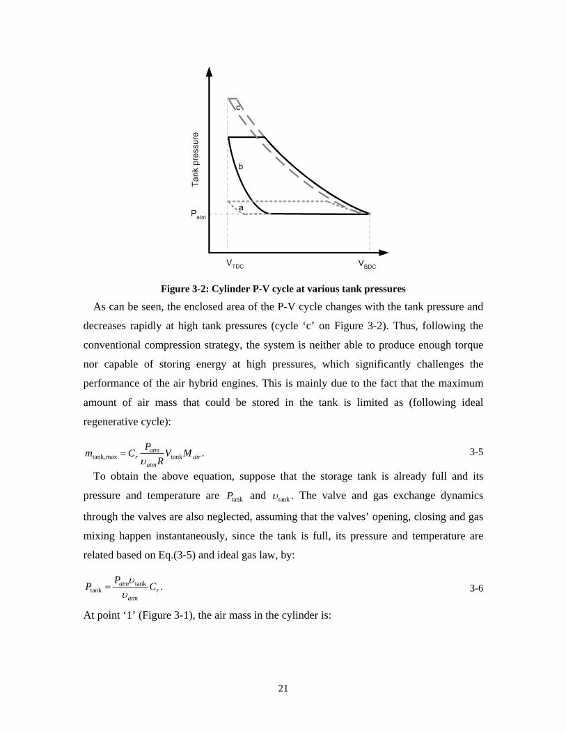
Figure 3-2: Cylinder P-V cycle at various tank pressures .................................................................... 21
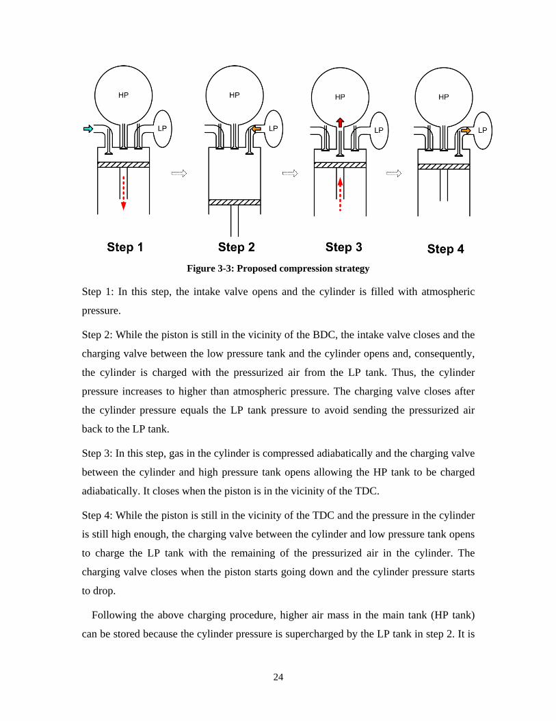
Figure 3-3: Proposed compression strategy ......................................................................................... 24
Figure 3-4: Double-tank regenerative ideal braking cycle ................................................................... 25
Figure 3-5: Vehicle velocity (a) and Tank pressure (b) ....................................................................... 27
Figure 3-6: Vehicle velocity (a) and Tank pressure (b) ....................................................................... 28
Figure 3-7: Cylinder geometrical parameters ...................................................................................... 28
Figure 3-8: Inlet flows to the cylinder ................................................................................................. 29
Figure 3-9: Flow through engine valves .............................................................................................. 30
Figure 3-10: Tank pressure vs. time ..................................................................................................... 33
Figure 3-11: Vehicle velocity vs. time ................................................................................................. 34
Figure 3-12: HP tank pressure vs. time ................................................................................................ 35
Figure 3-13: LP tank pressure vs. time ................................................................................................ 36
Figure 3-14: Vehicle velocity vs. time ................................................................................................. 36
Figure 4-1: Experimental set-up layout ............................................................................................... 39
Figure 4-2: Experimental setup ............................................................................................................ 40
Figure 4-3: Cylinder head configuration .............................................................................................. 41
Figure 4-4: Valve timing (a) Single-tank system, (b) Double-tank system ......................................... 42
Figure 4-5: HP tank pressure obtained from experiment ..................................................................... 44
Figure 4-6: HP tank pressure obtained from experiment ..................................................................... 45
Figure 4-7: LP tank pressure obtained from experiment ..................................................................... 45
Figure 4-8: HP tank pressure obtained from single-tank and double-tank systems ............................. 47
Figure 5-1: Brunel's first proposed air hybrid configuration [35] ........................................................ 49
Figure 5-2: Brunel's second proposed configuration for air hybrid engines [36] ................................ 49
ix
Figure 5-3: Proposed valvetrain based on Vtec .................................................................................... 51
Figure 5-4: Three-way valves arrangement in the conventional mode ................................................ 52
Figure 5-5: Three-way valves arrangement in the CB mode ................................................................ 53
Figure 5-6: Approximate Valve timings in the two-stroke modes ....................................................... 54
Figure 5-7: Three-way valves arrangement in the AM ........................................................................ 55
Figure 5-8: Cylinder head design for the double-tank configuration in the conventional mode .......... 56
Figure 5-9: Three-way valves arrangement in the compression braking mode .................................... 57
Figure 5-10: Approximate valve timings in the two-stroke modes ...................................................... 58
Figure 5-11: Three-way valves arrangement in the air motor mode .................................................... 59
Figure 5-12: Air tank pressure and temperature for the single-tank system ......................................... 62
Figure 5-13: Air tank pressure and temperature in for the double-tank system ................................... 63
Figure 5-14: Tank pressure in the startup mode ................................................................................... 65
Figure 5-15: Vehicle velocity during startup mode .............................................................................. 66
Figure 5-16: Engine speed during startup mode ................................................................................... 66
Figure 5-17: Modified experimental setup ........................................................................................... 67
Figure 5-18: Tank Pressure versus time for single-tank system ........................................................... 68
Figure 5-19: Cylinder head ................................................................................................................... 69
Figure 5-20: Cylinder P-V cycle at various tank pressures .................................................................. 70
Figure 5-21: Cylinder P-V cycle for single-tank and double-tank systems .......................................... 71
Figure 5-22: HP, LP and cylinder pressure for two subsequent cycles ................................................ 72
Figure 5-23: HP tank pressure versus time (42 [rpm]) ......................................................................... 73
Figure 5-24: HP tank pressure versus time (82 [rpm]) ......................................................................... 73
Figure 5-25: Engine speed at startup .................................................................................................... 75
Figure 5-26: Tank pressure in startup mode ......................................................................................... 75
Figure 5-27 Engine power in startup .................................................................................................... 76
Figure 6-1: Hybridized brake system ................................................................................................... 78
Figure 6-2: Comparison between the detailed model and MVM, a) throttle angle signal, b) mass flow
rate, c) manifold pressure, d) braking torque........................................................................................ 84
Figure 6-3: Engine volumetric efficiency in CB mode (@ 3000 [rpm]). ............................................. 85
Figure 6-4: Sliding mode controller scheme ........................................................................................ 93
Figure 6-5 Lookup table/PID controller scheme. ................................................................................. 94
Figure 6-6: Engine speed and tank pressure versus time ...................................................................... 95
x
Figure 6-7: Closed-loop tracking performance and controller commanded signal .............................. 95
Figure 6-8: Tracking error of ASMC, smooth SMC and high-gain PID without external disturbance 96
Figure 6-9: Tracking error of ASMC, smooth SMC and high-gain PID with external disturbance .... 97
Figure 6-10: Experimental setup .......................................................................................................... 99
Figure 6-11: Proportional valve effective area (suggested by manufacturer) .................................... 100
Figure 6-12: Engine braking torque versus tank pressure for various control signals ....................... 100
Figure 6-13: Experimental closed-loop tracking performance for ASMC, smooth SMC and PI ...... 102
Figure 6-14: Experimental closed-loop tracking performance for ASMC and PI ............................. 103
Figure 6-15: Change in the tank pressure throughout the experiment ............................................... 103
Figure 6-16: Actuator control signal .................................................................................................. 104
Figure 6-17: Experimental closed-loop tracking performance of ASMC, smooth SMC and PI ....... 105
Figure 6-18: Engine torque versus tank pressure for different control signals .................................. 106
Figure 6-19: Steady state LP tank pressure variation versus HP tank pressure ................................. 107
Figure 6-20: Experimental closed-loop tracking performance for ASMC and PI ............................. 108
Figure 6-21: LP tank pressure ............................................................................................................ 109
Figure 6-22: HP tank pressure for step input ..................................................................................... 109
Figure 7-1: Dynamic programming ................................................................................................... 113
Figure 7-2: a) Single-tank and, b) double-tank flow rate to the tank ................................................. 117
Figure 7-3: a) Single-tank and, b) double-tank braking torque .......................................................... 118
Figure 7-4: Air motor operating maps ............................................................................................... 119
Figure 7-5: UDDS operating map and single-tank regenerative operating range .............................. 120
Figure 7-6: UDDS Operating map and double-tank regenerative operating range ............................ 121
Figure 7-7: UDDS cycle a) speed profile, b) single-tank SoC profile, c) double-tank SoC profile .. 122
Figure 7-8: FT75 Operating map and single-tank regenerative operating range ............................... 123
Figure 7-9: FT75 Operating map and double-tank regenerative operating range .............................. 124
Figure 7-10: FTP75 cycle a) speed profile, b) single-tank SoC profile, c) double-tank SoC profile 125
xi
List of Tables Table 3-1 Simulated vehicle specifications .......................................................................................... 27
Table 3-2: Vehicle quarter model specifications ................................................................................. 32
Table 3-3: Single tank system valve timing ......................................................................................... 32
Table 3-4: Double tank system valve timing ........................................................................................ 34
Table 3-5 Simulation results ................................................................................................................. 36
Table 4-1: Engine and tanks’ characteristics ........................................................................................ 40
Table 4-2: Solenoid valves characteristics ........................................................................................... 41
Table 4-3: Solenoid valves activation .................................................................................................. 43
Table 4-4: Solenoid valves activation .................................................................................................. 44
Table 5-1 Vehicle and engine specifications ........................................................................................ 61
Table 5-2: Energy density of different energy sources [40] ................................................................. 64
Table 5-3: Valve timings ...................................................................................................................... 67
Table 6-1: Engine specification ............................................................................................................ 83
Table 6-2 Vehicle specifications .......................................................................................................... 91
Table 6-3: Controllers’ parameters ....................................................................................................... 92
Table 6-4: Torque Controller Performance .......................................................................................... 98
Table 6-5: Proportional valve characteristics ....................................................................................... 99
Table 6-6: Controllers' parameters ..................................................................................................... 102
Table 6-7: Controllers' performances ................................................................................................. 104
Table 7-1: Parameters of dynamic programming algorithm .............................................................. 114
Table 7-2: Vehicle and engine specification ...................................................................................... 115
Table 7-3: Fuel consumption in different cycles ................................................................................ 126

1
Nomenclature
a Piston stroke ( )θA Throttle effective area valveA Valve area
A Vehicle frontal area
cylA Cylinder instantaneous area
B Cylinder bore
dC Discharge/Drag coefficient
rC Compression ratio
vC Air specific heat
0C Sound speed C Engine heat capacity
pC Specific heat capacity d External disturbance e Tracking error E Estimation error f Final state F Discrete function
rf Rolling resistance coefficient
BrakingTrracF / Traction/Braking force g Gravitational acceleration
1g Knowledge of 1g 2g Knowledge of 2g
g~ Lumped model uncertainties estg~ Online estimate of g~
h Enthalpy per unit mass
K Controller proportional gain k Time step l Length of connecting rod
throttlem& Mass flow rate through the throttle
enginem& Mass flow rate to the engine [kg/s]
cylm Cylinder air mass
tankm Tank air mass
im Mass at point ‘i’
2
intakem& Cylinder inlet mass flow rate from intake manifold
LPm& Cylinder inlet mass flow rate from LP tank
HPm& Cylinder inlet mass flow rate from HP tank
airM Air average molecular mass
vehicleM Vehicle mass n System order
0P Ambient pressure
iP Pressure at point ‘i’
tankP Tank pressure
atmP Atmospheric pressure
LPP LP tank pressure
HPP HP tank pressure
cylP Cylinder pressure
inP Downstream pressure
outP Upstream pressure
rP Ratio of manifold pressure to ambient pressure mP Manifold pressure k
cylP Cylinder pressure after feeding kth storage
Q& Heat flux
r Tire radius
R Ideal gas constant S Sliding surface t Time
engineT Engine brake torque
fT Engine friction torque dT Desired torque
0U Environment internal energy U System internal energy
cylu Internal energy per unit mass of the gas inside the cylinder
tanku Internal energy per unit mass of the gas inside the tank
dV Engine displacement volume
0V System volume at equilibrium with environment V System volume
tankV Tank volume
LPV LP tank volume
HPV HP tank volume
3
cylV Cylinder volume *V Variable volume
1v Vehicle initial velocity
2v Vehicle final velocity v Mean piston speed
adW Adiabatic work
ijW Work from point ‘i’ to ‘j’
adW& Adiabatic power
isoW& Isentropic power
actW& Actual power
shaftW& Shaft power
kx System state x Independent variable
manν Manifold temperature
atmν Atmospheric temperature
0ν Ambient temperature
wallν Cylinder wall temperature
LPν LP temperature
HPν HP temperature ρ Air density δ Bound of Lumped uncertainty variation λ Positive constant ω Engine speed θ Crank angle
throttleθ Throttle angle [deg]
comthrottle,θ Commanded throttle angle [deg] ϕ Exergy
1ϕ Initial exergy of the system
2ϕ Final exergy of the system
h Heat transfer coefficient
adη Adiabatic efficiency
isoη Isentropic efficiency
mechη Mechanical efficiency
Regη Efficiency of Regeneration
volη Engine volumetric efficiency ε Boundary layer thickness
4
γ Adiabatic index Γ Controller adaptation gain Υ Lyapanov function
0ζ Environment entropy ζ System entropy
Φ Neural network FTP75 American driving cycle SoC State of Charge NEDC New European Driving Cycle CVO Charging valve opening CVC Charging valve closing IVO Intake valve opening IVC Intake valve closing TDC Top dead centre BDC Bottom dead centre LP Low pressure HP High pressure FMEP Friction mean effective pressure CAD Crank Angle Degree AM Air motor CB Compression braking
5
Chapter 1 Introduction
The automotive industry has been in a marathon of advancement over the past decade.
This is partly due to global environmental concerns about increasing air pollution and
decreasing fossil fuel resources. In 2006, the transportation sector comprised more than
135 million passenger cars in the United States representing the largest consumption of
energy [1]. Also, the sector has accounted for 28% of the green house emissions in the
United States [1]. Internal Combustion Engines (ICEs), the primary power source of
conventional vehicles, have a maximum efficiency of 30-40%. However, ICEs work at a
low efficiency level most of the time and, furthermore, the vehicle’s kinetic energy
cannot be recovered during braking and it is wasted.
1.1 Air Hybrid Vehicles
Air hybrid vehicles are founded on the same principle as hybrid electric ones. They
employ two energy sources, fuel and pressurized air, to propel the vehicle. During
braking, the kinetic energy of an air hybrid vehicle is converted into pressurized air by
running the same ICE in the compressor mode. Air hybrid engines can have four modes
of operation: Compression Braking (CB), Air Motor (AM), supercharged, and
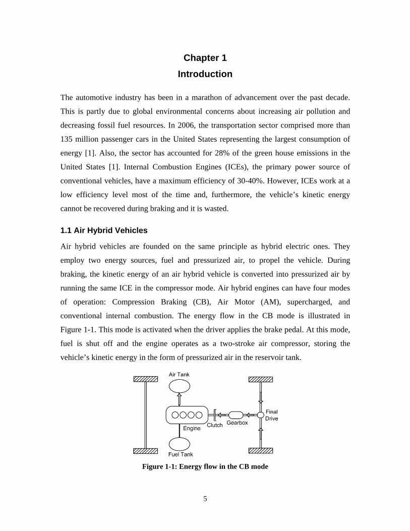
conventional internal combustion. The energy flow in the CB mode is illustrated in
Figure 1-1. This mode is activated when the driver applies the brake pedal. At this mode,
fuel is shut off and the engine operates as a two-stroke air compressor, storing the
vehicle’s kinetic energy in the form of pressurized air in the reservoir tank.
Figure 1-1: Energy flow in the CB mode
6
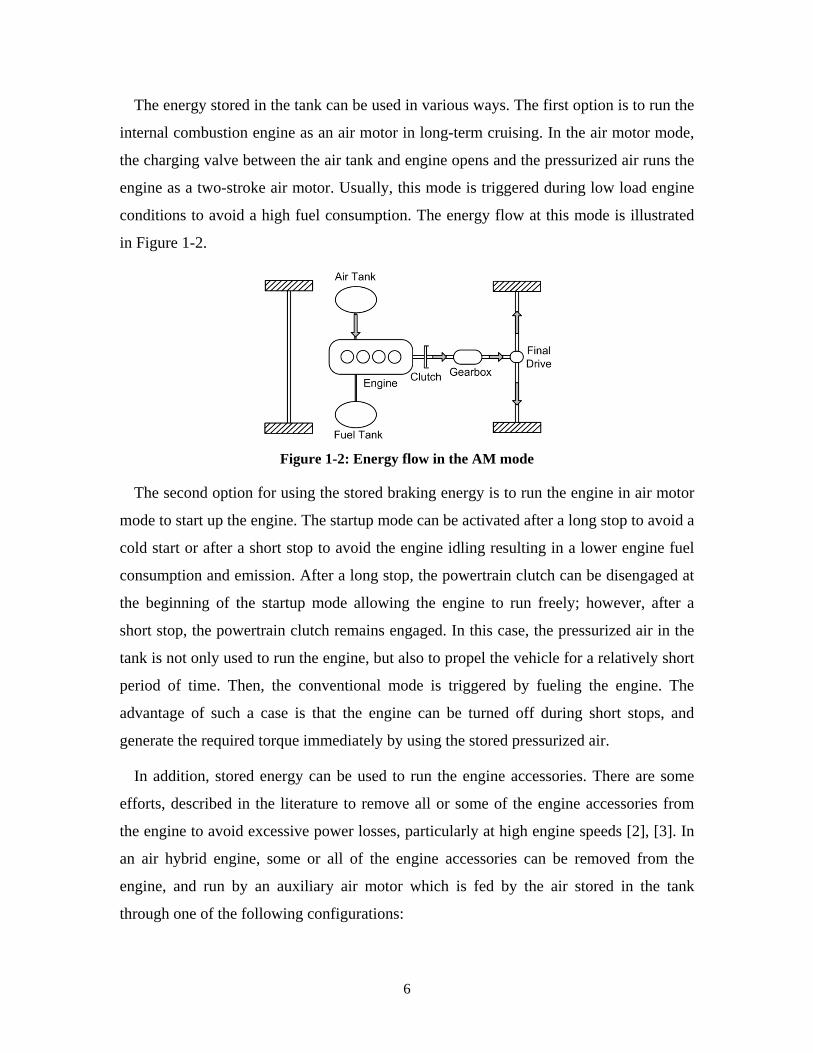
The energy stored in the tank can be used in various ways. The first option is to run the
internal combustion engine as an air motor in long-term cruising. In the air motor mode,
the charging valve between the air tank and engine opens and the pressurized air runs the
engine as a two-stroke air motor. Usually, this mode is triggered during low load engine
conditions to avoid a high fuel consumption. The energy flow at this mode is illustrated
in Figure 1-2.
Figure 1-2: Energy flow in the AM mode
The second option for using the stored braking energy is to run the engine in air motor
mode to start up the engine. The startup mode can be activated after a long stop to avoid a
cold start or after a short stop to avoid the engine idling resulting in a lower engine fuel
consumption and emission. After a long stop, the powertrain clutch can be disengaged at
the beginning of the startup mode allowing the engine to run freely; however, after a
short stop, the powertrain clutch remains engaged. In this case, the pressurized air in the
tank is not only used to run the engine, but also to propel the vehicle for a relatively short
period of time. Then, the conventional mode is triggered by fueling the engine. The
advantage of such a case is that the engine can be turned off during short stops, and
generate the required torque immediately by using the stored pressurized air.
In addition, stored energy can be used to run the engine accessories. There are some
efforts, described in the literature to remove all or some of the engine accessories from
the engine to avoid excessive power losses, particularly at high engine speeds [2], [3]. In
an air hybrid engine, some or all of the engine accessories can be removed from the
engine, and run by an auxiliary air motor which is fed by the air stored in the tank
through one of the following configurations:
7
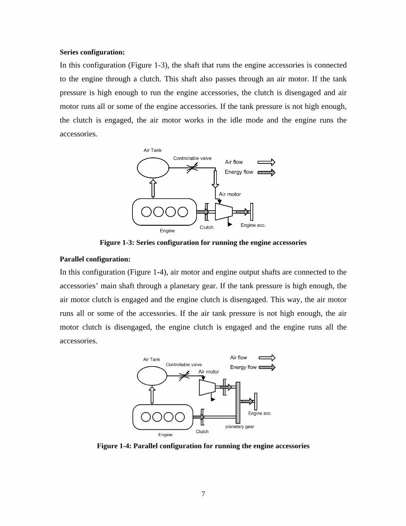
Series configuration:
In this configuration (Figure 1-3), the shaft that runs the engine accessories is connected
to the engine through a clutch. This shaft also passes through an air motor. If the tank
pressure is high enough to run the engine accessories, the clutch is disengaged and air
motor runs all or some of the engine accessories. If the tank pressure is not high enough,
the clutch is engaged, the air motor works in the idle mode and the engine runs the
accessories.
Figure 1-3: Series configuration for running the engine accessories
Parallel configuration:
In this configuration (Figure 1-4), air motor and engine output shafts are connected to the
accessories’ main shaft through a planetary gear. If the tank pressure is high enough, the
air motor clutch is engaged and the engine clutch is disengaged. This way, the air motor
runs all or some of the accessories. If the air tank pressure is not high enough, the air
motor clutch is disengaged, the engine clutch is engaged and the engine runs all the
accessories.
Figure 1-4: Parallel configuration for running the engine accessories
8
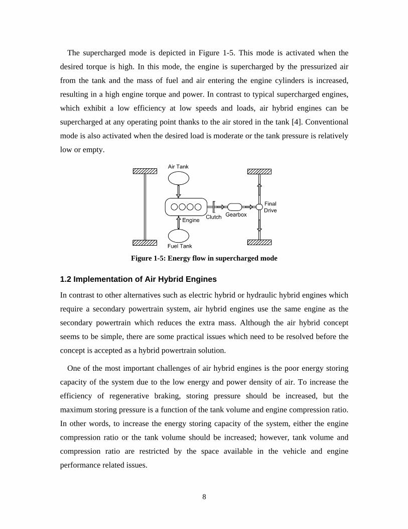
The supercharged mode is depicted in Figure 1-5. This mode is activated when the
desired torque is high. In this mode, the engine is supercharged by the pressurized air
from the tank and the mass of fuel and air entering the engine cylinders is increased,
resulting in a high engine torque and power. In contrast to typical supercharged engines,
which exhibit a low efficiency at low speeds and loads, air hybrid engines can be
supercharged at any operating point thanks to the air stored in the tank [4]. Conventional
mode is also activated when the desired load is moderate or the tank pressure is relatively
low or empty.
Figure 1-5: Energy flow in supercharged mode
1.2 Implementation of Air Hybrid Engines
In contrast to other alternatives such as electric hybrid or hydraulic hybrid engines which
require a secondary powertrain system, air hybrid engines use the same engine as the
secondary powertrain which reduces the extra mass. Although the air hybrid concept
seems to be simple, there are some practical issues which need to be resolved before the
concept is accepted as a hybrid powertrain solution.
One of the most important challenges of air hybrid engines is the poor energy storing
capacity of the system due to the low energy and power density of air. To increase the
efficiency of regenerative braking, storing pressure should be increased, but the
maximum storing pressure is a function of the tank volume and engine compression ratio.
In other words, to increase the energy storing capacity of the system, either the engine
compression ratio or the tank volume should be increased; however, tank volume and
compression ratio are restricted by the space available in the vehicle and engine
performance related issues.
9
The other challenge in the implementation of an air hybrid engine is the inevitability of
using flexible valvetrains. Since an air hybrid engine has different operational modes, a
flexible valvetrain is needed for the implementation of the concept. Although
conventional valvetrains limit the engine’s performance and cannot practically be used in
an air hybrid engine, they have operational advantages, because the valve motion is
governed by a cam profile, designed to confine the valve seating velocity and lift [5]. In
contrast, a flexible camless valvetrain with no direct mechanical connection with the
engine introduces control complexities, a high power consumption, and an increased cost
into the system. Several ongoing studies address the technical challenges of using fully
flexible valvetrains [6], [7] [8].
In addition, the implementation of torque control in an air hybrid engine during the
AM, CB, and supercharged modes has not been addressed by any researcher so far. To
implement an air hybrid engine, the engine configuration should be further modified to
control the engine torque in the AM and CB modes. Furthermore, a robust controller for
adjusting the torque should be developed.
1.3 Research Objectives and Thesis Layout
Although there are many challenges there are also many advantages in the
implementation and commercialization of air hybrid engines. This research is intended to
address some of these challenges by focusing on improving the overall efficiency and
reducing the complexity in the valve system and torque control of air hybrid engines.
The objectives of this thesis, in general, are:
1. Development and testing a novel compression strategy to increase the energy
storing capacity of regenerative braking system in air hybrid engines.
2. Development and testing a cam-based valvetrain and cylinder head structure to
relax the need for a fully flexible valvetrain.
3. Design and implementation of an engine torque controller for regenerative
braking mode.
4. Evaluation of the overall efficiency of the proposed air hybrid engine in various
standard drive cycles.
10
This thesis is organized in eight chapters and nine appendixes. Chapter 1 provides an
introduction to air hybrid engines and the objectives of this thesis. Ongoing studies in
different aspects of air hybrid engines are addressed in Chapter 2. Chapter 3 introduces a
new compression process using two air tanks for the regenerative braking system, and
presents a comparison between the conventional and developed compression processes.
Chapter 4 describes experimental studies and results of the proposed compression
strategy. A novel cam-based valvetrain for conventional and proposed air hybrid
configurations is developed and assessed using simulation and experimental studies in
Chapter 5. Chapter 6 is devoted to the design and implementation of model-based and
model-free regenerative braking torque controllers. Chapter 7 presents the drive cycle
simulation and provides a comparison between the conventional and proposed air hybrid
engines based on their optimized mode scheduling. Chapter 8 summarizes the
contributions and provides some suggestions for future work.
11
Chapter 2 Literature Review
Powertrains can be divided into two groups, according to the number of their energy
sources: single-source vehicles such as gas, diesel, pure electric and compressed air
vehicles, and double-source vehicles such as electric and air hybrid vehicles. In this
chapter, the investigations on air hybrid vehicles are discussed in detail.
2.1 Air Hybrid Vehicles
Hybrid Electric Vehicles (HEVs) have overcome production limits and are regarded as
one of the most effective and feasible solutions to current environmental concerns. HEVs
use two sources of energy: fossil fuel and electrochemical energy stored in batteries.
They are usually comprised of an ICE and an electric motor. HEVs are able to store the
vehicle’s kinetic energy in the shape of electrochemical energy in a battery by running
the electric motor as a generator. Despite the beneficiary improvements that this kind of
vehicle provides, there are some serious concerns about HEVs performance. The HEV
powertrain system is complex, which introduces a very complicated control problem and
increases the maintenance cost of the vehicle. Using a battery in the powertrain is also a
drawback for HEVs because battery-charging efficiency is highly dependent to the
charging strategy [9], the state of charge of the battery (which forms the basis of vehicle
control strategy) cannot be precisely defined [10]. In addition, HEVs are 10% to 30%
heavier than ICE-based vehicles [11].
Compared with a hybrid electric vehicle, an air hybrid-based vehicle could provide a
better efficiency with less complexity, weight and cost. In 1999, Schechter [12] proposed
the idea of an air hybrid engine for the first time. The idea evolved from the fact that the
internal combustion engine can be run as a compressor and an air motor by changing the
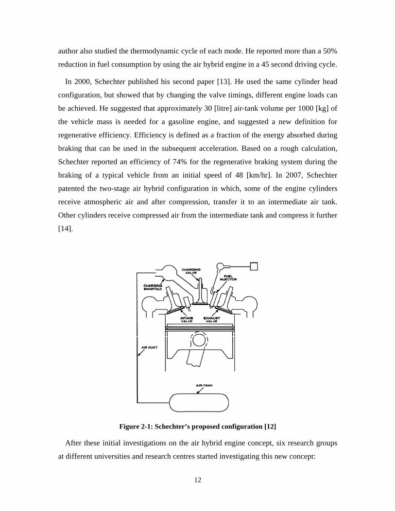
valve timing. Schechter [12] has introduced a new cylinder head configuration in which
there is an extra valve connecting the cylinder to an air tank, called the charging valve.
This extra valve is active only when the engine works as a compressor or air motor. The
valve sends the pressurized air from the cylinder to the air tank, and vice versa. The
12
author also studied the thermodynamic cycle of each mode. He reported more than a 50%
reduction in fuel consumption by using the air hybrid engine in a 45 second driving cycle.
In 2000, Schechter published his second paper [13]. He used the same cylinder head
configuration, but showed that by changing the valve timings, different engine loads can
be achieved. He suggested that approximately 30 [litre] air-tank volume per 1000 [kg] of
the vehicle mass is needed for a gasoline engine, and suggested a new definition for
regenerative efficiency. Efficiency is defined as a fraction of the energy absorbed during
braking that can be used in the subsequent acceleration. Based on a rough calculation,
Schechter reported an efficiency of 74% for the regenerative braking system during the
braking of a typical vehicle from an initial speed of 48 [km/hr]. In 2007, Schechter
patented the two-stage air hybrid configuration in which, some of the engine cylinders
receive atmospheric air and after compression, transfer it to an intermediate air tank.
Other cylinders receive compressed air from the intermediate tank and compress it further
[14].
Figure 2-1: Schechter’s proposed configuration [12]
After these initial investigations on the air hybrid engine concept, six research groups
at different universities and research centres started investigating this new concept:
13
1. UCLA in collaboration with Ford Motor Company.
2. Lund Institute of Technology.
3. Brunel University.
4. Institute PRISME/ EMP Université d’Orléans.
5. ETH University.
6. National Taipei University of Technology.
In the next section the work of each research group is reviewed.
2.1.1 UCLA Research Group
In 2003, Chun Tai et al., in collaboration with Ford Motor Company [15], proposed a
new cylinder head configuration which enabled different modes of operation without
adding an extra valve to the head. The group utilized four fully flexible camless valves
for each cylinder, two intakes, and two exhausts. In this configuration, one of the intake
valves is switchable, and connects either the intake manifold or air tank to the cylinder by
a three-way valve. The group also optimized the valve timings according to the desired
load, the tank pressure, and speed. The researchers claimed a 64% and 12% fuel economy
improvement in city and highway driving, respectively. This improvement is reported to
be partly due to using the camless valvetrain which permitted the engine to run
unthrottled. The authors have provided no experimental results, but did use GT-POWER
to simulate the proposed air hybrid engine configuration.
In 2008, Kang et al. [16] published their first experimental work on an air hybrid
engine in collaboration with Volvo and Sturman Industries. They converted a six-cylinder
diesel engine to an air hybrid engine utilizing a Sturman hydraulic camless valvetrain.
They optimized the valve timings of the AM and CB modes at two engine speeds and
three tank pressures, and implemented the obtained valve timings experimentally. They
also reported the transient performance of the engine in switching from the CB to the AM
mode.
14
In a dissertation submitted by one of the group members [17], the concept of using a
double-stage regenerative braking, initially introduced by Schechter in 2007, was
compared to a single-stage system in simulations
2.1.2 Lund Institute of Technology
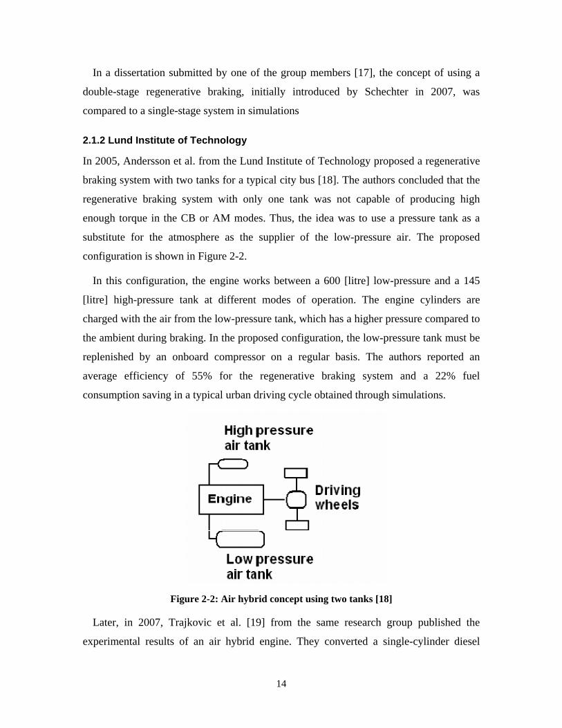
In 2005, Andersson et al. from the Lund Institute of Technology proposed a regenerative
braking system with two tanks for a typical city bus [18]. The authors concluded that the
regenerative braking system with only one tank was not capable of producing high
enough torque in the CB or AM modes. Thus, the idea was to use a pressure tank as a
substitute for the atmosphere as the supplier of the low-pressure air. The proposed
configuration is shown in Figure 2-2.
In this configuration, the engine works between a 600 [litre] low-pressure and a 145
[litre] high-pressure tank at different modes of operation. The engine cylinders are
charged with the air from the low-pressure tank, which has a higher pressure compared to
the ambient during braking. In the proposed configuration, the low-pressure tank must be
replenished by an onboard compressor on a regular basis. The authors reported an
average efficiency of 55% for the regenerative braking system and a 22% fuel
consumption saving in a typical urban driving cycle obtained through simulations.
Figure 2-2: Air hybrid concept using two tanks [18]
Later, in 2007, Trajkovic et al. [19] from the same research group published the
experimental results of an air hybrid engine. They converted a single-cylinder diesel
15
engine to an air hybrid engine. Pneumatic valve actuators were used to make the air
hybrid configuration possible. Two modes, CB and AM, were tested and studied in this
work. The Engine’s Indicated Mean Effective Pressure (IMEP) and tank pressure were
reported for different valve timings and engine speeds at the AM and CB modes. A new
definition for efficiency was also presented, based on the negative and positive IMEP at
the CB and consequent AM modes. An efficiency of 33% for the regenerative braking
system was reported.
Trajkovic et al. [20] published their second investigation on the same air hybrid engine
in 2008. They optimized the valve timings for the CB and AM modes at various tank
pressures. Additionally, they modified the tank valve diameter to increase the system
efficiency. They showed that, by using a larger charging valve, the efficiency of the
regenerative system, based on their definition of efficiency, could be increased to
approximately 44%. They also compared the experimental results with GT-POWER
results and found them to be in agreement.
In their next study, the authors validated an engine model in GT-Power by the
experimental results and used the GT-Power model to study the effect of different
parameters such as tank valve diameter and valve timings on pneumatic hybrid
performance [20]. In 2010, they published the driving cycle simulation results of their
single-cylinder air hybrid engine. They chose a lower limit of 8 [bar] for the tank pressure
and reported a reduction in the fuel consumption up to 30% in the Braunschweig driving
cycle [21].
2.1.3 Brunel University
In 2009, Hua Zhao’s group from Brunel University proposed four stroke air modes for an
air hybrid engine. To implement the concept without using a camless valvetrain, a new
valve configuration was proposed utilizing a Cam Profile Switching (CPS) system for the
operational mode switching, a controllable solenoid valve for managing the amount of air
entering or exiting the air tank, and a variable valve timing system to shift the valve
events without changing the valve duration. They reported a regenerative braking
efficiency of 15% from the simulations, but the need for a high speed solenoid valve was
a substantial drawback of the proposed design. Later in 2010, the team tackled the
16
problem by introducing two new designs for air hybrid engines. In one of their designs,
the researchers introduced and extra check valve between the tank and one of the intake
valves, and a butterfly valve in the intake manifold to eliminate the need for a high speed
solenoid valve. In their other design, they proposed a valvetrain with the intake opening
duration of 360 degrees and a check valve between the intake manifold and the intake
valves. Their proposed configurations will be discussed in more detail in Chapter 5.
2.1.4 Institute PRISME/ EMP Université d’Orléans
P. Higelin et al. [6] published their work on the air hybrid concept in 2003. They
presented a thermodynamic model of each operational mode, and also adopted a set of
operating mode selection rules, based on the tank pressure and vehicle speed. The
optimized values for the tank volume and maximum allowable tank pressure were
defined based on NEDC cycle simulation results. The author reported a 15% fuel saving
in NEDC driving cycle. They proposed and compared different energy management
strategies in their work in 2009 [22].
2.1.5 ETH University
Guzzella et al. [4], [23] proposed and conducted experiments on the four-stroke air
hybrid engine to eliminate the need for a complete set of fully camless valves. In their
proposed configuration, the intake and exhaust valves remained camshaft-driven but an
extra camless valve connecting the cylinder to the tank was added. They classified the air
tank as an ultra short-term storage device due to the low energy density of pressurized air.
They concluded that the best way to use the tank-pressurized air was to supercharge the
engine. Since the engine could be supercharged even at low torques and speeds, a larger
engine can be downsized in an air hybrid vehicle and there is no need to design the
engine turbocharger for an optimal dynamic performance. Thus, the supercharged mode
is activated whenever a sudden increase in the engine torque is required until the
supercharger reaches the steady state condition and as a result, the turbo lag is eliminated.
This was reported to be the most important advantage of air hybrid engines, leading to
25-35% reduction in fuel consumption, compared with that of a typical engine. They
proposed the concept of a cold air tank in contrast to an insulated, hot tank proposed in
17
[12] to reduce the knock probability. The team was successful in running the air hybrid
engine in all operational modes, including conventional mode.
They employed the Dynamic Programming (DP) algorithm to find the optimum mode
scheduling for the air hybrid vehicle in a drive cycle and also conduct a comparison
between different hybrid structures in [24].
2.1.6 National Taipei University of Technology
In addition to the aforementioned air hybrid structures, there is also a totally different
configuration of an air hybrid, proposed by Huang [25] in 2004. In this configuration, a
typical ICE was connected to a screw compressor and operates at the engine’s most
efficient point. Then, a pneumatic motor is driven by the compressed air to generate
power. Thus, the main difference between the proposed air hybrid configuration and a
series hybrid electric vehicle is that an air compressor replaces the generator, a pneumatic
motor replaces the electric motor, and a high-pressure air tank replaces the battery.
Huang achieved an 18% improvement in efficiency, compared with that of an ICE-based
powertrain. However, the author has not considered the effect of the vehicle weight
increase (due to adding extra components such as pneumatic motor and compressor) on
the overall efficiency of the vehicle. The author reported his proposed system’s
experimental results in [26] and [27].
2.2 Summary
In this chapter, a literature survey on the concept of air hybrid engines was presented.
The concept is not new; however, the practical challenges in implementing the concept
have prevented researchers from exploiting its potential to increase the powertrain
efficiency. Except for the ETH research group who was successful in running the engine
in various modes, most of the experimental work has been limited to testing regenerative
or air motor modes of an air hybrid engine. Although some substitute valvetrain
configurations have been suggested to avoid a camless valvetrain in theory, all
experimental work is based on camless valvetrain in the literature.
18
Chapter 3 Double-tank Compression Strategy
A significant fraction of energy is wasted in braking in a typical city driving cycle, where
stop-and-go driving patterns are common. For instance, in the FTP75 urban driving cycle
approximately 40% of the energy is wasted while braking [28]. Thus, if the braking
energy can be recovered, the vehicle energy consumption can be significantly reduced
[28]. The main motivation to hybridize a vehicle’s powertrain is to capture and reuse the
energy wasted during braking. Air hybrid vehicles can capture and store braking energy
in the form of pressurized air for further use.
3.1 Efficiency of Energy Storing
As mentioned, an internal combustion engine works as a simple compressor during
regenerative braking. Although there are several efficiency definitions for compressors,
such as volumetric, adiabatic, isothermal, isentropic and mechanical efficiency
(Appendix A), none of them represents the ratio of the stored energy in the tank to the
consumed energy. The efficiency of regenerative braking should be represented in terms
of energy stored in the tank to the change in the kinetic energy of the decelerating
vehicle. While stored energy in the tank cannot be expressed by internal energy of the
stored air (as it does not represent the ability of stored gas to perform work), it can be
expressed by the exergy of the stored gas. Exergy, or availability of a system, is defined
as the maximum useful work of a process which brings the system to equilibrium with
the environment, and can be expressed by the following relation [29]:
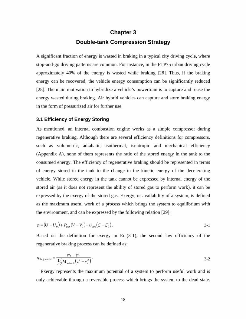
( ) ( ) ( ) .000 ζζυϕ −−−+−= atmatm VVPUU 3-1
Based on the definition for exergy in Eq.(3-1), the second law efficiency of the
regenerative braking process can be defined as:
( ) .2
1 22
21
12storedReg, vvM vehicle −
−=
ϕϕη 3-2
Exergy represents the maximum potential of a system to perform useful work and is
only achievable through a reversible process which brings the system to the dead state.
19
The dead state is a condition at which the system has the same pressure and temperature
as those of the surroundings. However, in the case of a regenerative braking system, the
stored energy in the tank is used later through an adiabatic expansion which brings the
system only to pressure equilibrium with the environment, not thermal equilibrium. This
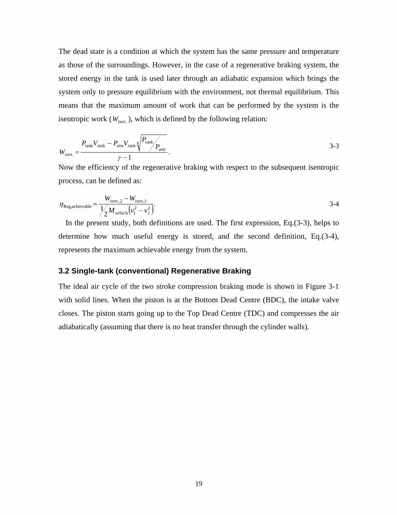
means that the maximum amount of work that can be performed by the system is the
isentropic work ( .isenW ), which is defined by the following relation:
.1
tanktanktanktank
. −
−=
γ
katm
atm
isenP
PVPVPW
3-3
Now the efficiency of the regenerative braking with respect to the subsequent isentropic
process, can be defined as:
( ).21 2
221
1.,2.,achievableReg, vvM
WW
vehicle
isenisen
−
−=η 3-4
In the present study, both definitions are used. The first expression, Eq.(3-3), helps to
determine how much useful energy is stored, and the second definition, Eq.(3-4),
represents the maximum achievable energy from the system.
3.2 Single-tank (conventional) Regenerative Braking
The ideal air cycle of the two stroke compression braking mode is shown in Figure 3-1
with solid lines. When the piston is at the Bottom Dead Centre (BDC), the intake valve
closes. The piston starts going up to the Top Dead Centre (TDC) and compresses the air
adiabatically (assuming that there is no heat transfer through the cylinder walls).
20
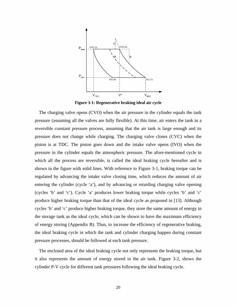
Figure 3-1: Regenerative braking ideal air cycle
The charging valve opens (CVO) when the air pressure in the cylinder equals the tank
pressure (assuming all the valves are fully flexible). At this time, air enters the tank in a
reversible constant pressure process, assuming that the air tank is large enough and its
pressure does not change while charging. The charging valve closes (CVC) when the
piston is at TDC. The piston goes down and the intake valve opens (IVO) when the
pressure in the cylinder equals the atmospheric pressure. The afore-mentioned cycle in
which all the process are reversible, is called the ideal braking cycle hereafter and is
shown in the figure with solid lines. With reference to Figure 3-1, braking torque can be
regulated by advancing the intake valve closing time, which reduces the amount of air
entering the cylinder (cycle ‘a’), and by advancing or retarding charging valve opening
(cycles ‘b’ and ‘c’). Cycle ‘a’ produces lower braking torque while cycles ‘b’ and ‘c’
produce higher braking torque than that of the ideal cycle as proposed in [13]. Although
cycles ‘b’ and ‘c’ produce higher braking torque, they store the same amount of energy in
the storage tank as the ideal cycle, which can be shown to have the maximum efficiency
of energy storing (Appendix B). Thus, to increase the efficiency of regenerative braking,
the ideal braking cycle in which the tank and cylinder charging happen during constant
pressure processes, should be followed at each tank pressure.
The enclosed area of the ideal braking cycle not only represents the braking torque, but
it also represents the amount of energy stored in the air tank. Figure 3-2, shows the
cylinder P-V cycle for different tank pressures following the ideal braking cycle.
21
Figure 3-2: Cylinder P-V cycle at various tank pressures As can be seen, the enclosed area of the P-V cycle changes with the tank pressure and
decreases rapidly at high tank pressures (cycle ‘c’ on Figure 3-2). Thus, following the
conventional compression strategy, the system is neither able to produce enough torque
nor capable of storing energy at high pressures, which significantly challenges the
performance of the air hybrid engines. This is mainly due to the fact that the maximum
amount of air mass that could be stored in the tank is limited as (following ideal
regenerative cycle):
.tankmax,tank airatm
atmr MV
RPCmυ
= 3-5
To obtain the above equation, suppose that the storage tank is already full and its
pressure and temperature are tankP and tankυ . The valve and gas exchange dynamics
through the valves are also neglected, assuming that the valves’ opening, closing and gas
mixing happen instantaneously, since the tank is full, its pressure and temperature are
related based on Eq.(3-5) and ideal gas law, by:
.tanktank r
atm
atm CPPυυ
= 3-6
At point ‘1’ (Figure 3-1), the air mass in the cylinder is:
22
.1 airatm
cylatm MR
VPm
υ= 3-7
Considering adiabatic compression and ideal mixing of gases when the charging valve
is opened, cylinder pressure at arbitrary point ‘2’ where the cylinder volume is *V , (this
point may not be necessarily the point where the cylinder pressure equals the tank
pressure), is:
,tank
*
tanktank*
*
2 VV
CVPVVV
PP
ratm
atmcylatm
+
+⎟⎟⎠
⎞⎜⎜⎝
⎛
=υυ
γ
3-8
and the temperature at point ‘2’ is:
.
tank1
*
**
tanktank*
*
2
ratm
atm
cylatm
cylatm
ratm
atmcylatm
CVP
VV
VVV
P
CVPVVV
P
υυ
υυ
υ
γ
γ
γ
+
⎟⎟⎠
⎞⎜⎜⎝
⎛
⎟⎟⎠
⎞⎜⎜⎝
⎛
+⎟⎟⎠
⎞⎜⎜⎝
⎛
=
−
3-9
Air pressure and temperature at point ‘3’ are defined by:
,
tank
*tank
23
γ
⎟⎟⎟⎟⎟
⎠
⎞
⎜⎜⎜⎜⎜
⎝
⎛
+
+=
r
cyl
CV
V
VVPP 3-10
.
1
tank
*tank
23
−
⎟⎟⎟⎟⎟
⎠
⎞
⎜⎜⎜⎜⎜
⎝
⎛
+
+=
γ
υυ
r
cyl
CV
V
VV 3-11
The charging valve closes at point ‘3’ so the amount of air mass trapped in the cylinder
dead volume can be found as follows:
.3
3
airr
cyl
cyl MR
CV
Pm
υ= 3-12
Now if we plug Eqs.(3-10) and (3-11) into Eq.(3-12), the trapped mass in the cylinder
after closing the charging valve will be:
23
,airatm
cylatmcyl M
RVP
mυ
= 3-13
which equals the amount of air mass entered into the cylinder at point ‘1’ (Eq. (3-7)).
This means that no air can be stored in the tank if the amount of the air mass in the tank
equals to what is shown by Eq.(3-5). Since the maximum amount of air mass in the air
tank is limited, to increase the energy storing ability of the system, tank temperature
should be kept as high as possible. Although higher tank temperature increases the
storing pressure and, consequently, increases the energy storing capacity of the system,
tank temperature should be bounded because it increases the engine body temperature
and causes pre-ignition in the cylinder. Thus, the storing pressure and energy storing
capacity of the regenerative system are also bounded. For an air hybrid engine with the
compression ratio of 10 and maximum tank temperature of 450[K], the maximum
achievable tank pressure is about 15[bar]. Considering these results, the maximum energy
storing capacity of a pneumatic regenerative braking system is about 1.57[kJ/litre].
Compared to the energy density of Lithium-ion batteries which is about 700-
1000[kJ/Litre] [28,30,31], the pneumatic regenerative braking system’s ability to store
energy is insignificant. Based on Eq.(3-5), there are two options to increase the capacity
of energy storing of the air tank – either using a larger tank or increasing the compression
ratio. Increasing the volume of the tank is not a viable solution due to space limitation in
the vehicle. Likewise, increasing the compression ratio of the cylinder is not achievable
because of engine performance limitations. However, the system overall compression
ratio can be increased indirectly if a multi-tank compression technique is employed.
3.3 Double-tank Regenerative Braking
The double-tank regenerative system is comprised of two storage tanks, one small in size,
low pressure tank (LP) and one large in size, high pressure tank (HP), as shown in Figure
3-3. With reference to this figure, the four steps of a cycle are defined as follows:
24
Figure 3-3: Proposed compression strategy
Step 1: In this step, the intake valve opens and the cylinder is filled with atmospheric
pressure.
Step 2: While the piston is still in the vicinity of the BDC, the intake valve closes and the
charging valve between the low pressure tank and the cylinder opens and, consequently,
the cylinder is charged with the pressurized air from the LP tank. Thus, the cylinder
pressure increases to higher than atmospheric pressure. The charging valve closes after
the cylinder pressure equals the LP tank pressure to avoid sending the pressurized air
back to the LP tank.
Step 3: In this step, gas in the cylinder is compressed adiabatically and the charging valve
between the cylinder and high pressure tank opens allowing the HP tank to be charged
adiabatically. It closes when the piston is in the vicinity of the TDC.
Step 4: While the piston is still in the vicinity of the TDC and the pressure in the cylinder
is still high enough, the charging valve between the cylinder and low pressure tank opens
to charge the LP tank with the remaining of the pressurized air in the cylinder. The
charging valve closes when the piston starts going down and the cylinder pressure starts
to drop.
Following the above charging procedure, higher air mass in the main tank (HP tank)
can be stored because the cylinder pressure is supercharged by the LP tank in step 2. It is
25
important to note that this strategy is different from a multi-stage compression strategy
since it only needs one cylinder and the compression cycle is completed in only one
revolution of the crank shaft. This results in doubling the flow rate to the air tank
compared to the double-stage strategy proposed by Schechter [14]. It has to be mentioned
that as the case of double-stage compression strategy in which air is cooled down
between the stages to increase the overall efficiency of the system, in double-tank
compression strategy the LP tank should be cooled down to increase the mass flow rate
from the LP to the cylinder and, consequently, to increase the energy storing efficiency of
the system.
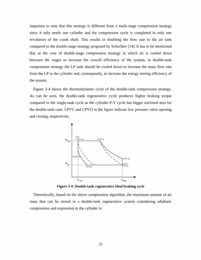
Figure 3-4 shows the thermodynamic cycle of the double-tank compression strategy.
As can be seen, the double-tank regenerative cycle produces higher braking torque
compared to the single-tank cycle as the cylinder P-V cycle has bigger enclosed area for
the double-tank case. LPVC and LPVO in the figure indicate low pressure valve opening
and closing, respectively.
Figure 3-4: Double-tank regenerative ideal braking cycle
Theoretically, based on the above compression algorithm, the maximum amount of air
mass that can be stored in a double-tank regenerative system considering adiabatic
compression and expression in the cylinder is:
26
.1
1tank
max,tank air
cyl
LP
cyl
LPr
ratm
atm M
VV
VVC
CR
VPm
⎟⎟⎟⎟⎟
⎠
⎞
⎜⎜⎜⎜⎜
⎝
⎛
+
+
=υ
3-14
To prove the above equation we consider Figure 3-4 again. It is assumed that the LP
tank is cooled down to the environment temperature. The maximum LP pressure when
both of the tanks are completely full, is defined by the following relation (For more
details see Appendix C):
.ratmLP CPP = 3-15
Assuming an ideal mixing process, the cylinder pressure at point ‘2’, after supercharging
the engine with the LP tank pressurized air, is:
.2LPcyl
LPLPcylatm
VVVPVP
P+
+= 3-16
Since HP tank is already full, we can assume that the charging valve opens and closes
precisely at TDC. Thus, pressure and temperature at point ‘4’ will be defined by:
,4,3γ
rLPcyl
LPLPcylatm CVV
VPVPP
+
+= 3-17
.14,3
−= γυυ ratmC 3-18
Since the HP tank is full, 4,3PPHP = , thus, the maximum amount of mass stored in the HP
tank becomes:
.1
1tank
4
tank4maxtank, air
cyl
LP
cyl
LPr
ratm
atmair M
VV
VVC
CR
VPMRVPm
⎟⎟⎟⎟⎟
⎠
⎞
⎜⎜⎜⎜⎜
⎝
⎛
+
+
==υυ 3-19
Considering K][450max, =HPυ , cylLP VV = and 10=rC , the maximum pressure could go
up to 82.5[bar], which is a considerable improvement compared to 15[bar].
Consequently, the aforementioned double-tank compression technique can increase the
energy density of the main storage by a factor of 8.5 (based on the definition for
efficiency given in Eq. (3-4)).
27
3.4 Simulations
The above-mentioned compression processes are used to simulate and compare the
single-tank and the double-tank regenerative braking of a quarter vehicle model with the
specifications shown in Table 3-1. It is assumed that the vehicle decelerates from
60[km/hr] only by using regenerative braking and no energy is lost due to engine friction,
vehicle resistance or any other source of energy losses. The LP tank in the double-tank
system is assumed to be cooled down to the environment temperature. In these
simulations, the valve and gas exchange dynamics through the valves are neglected.
Table 3-1 Simulated vehicle specifications Vehicle Mass 450 [kg] Engine Type Single Cylinder Cylinder Volume 500 [cc] Storage Tank Volume 7.5 [l] Compression Ratio 10 Storage Tank Initial Pressure 1 [bar] Maximum Tank Temperature 450 [k] LP Tank Volume 0.5 [l]
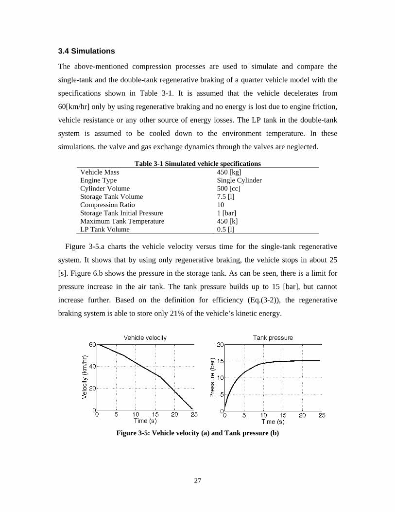
Figure 3-5.a charts the vehicle velocity versus time for the single-tank regenerative
system. It shows that by using only regenerative braking, the vehicle stops in about 25
[s]. Figure 6.b shows the pressure in the storage tank. As can be seen, there is a limit for
pressure increase in the air tank. The tank pressure builds up to 15 [bar], but cannot
increase further. Based on the definition for efficiency (Eq.(3-2)), the regenerative
braking system is able to store only 21% of the vehicle’s kinetic energy.
Figure 3-5: Vehicle velocity (a) and Tank pressure (b)
28
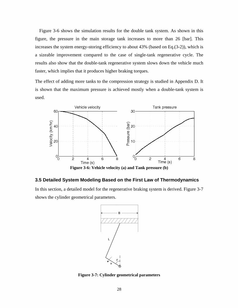
Figure 3-6 shows the simulation results for the double tank system. As shown in this
figure, the pressure in the main storage tank increases to more than 26 [bar]. This
increases the system energy-storing efficiency to about 43% (based on Eq.(3-2)), which is
a sizeable improvement compared to the case of single-tank regenerative cycle. The
results also show that the double-tank regenerative system slows down the vehicle much
faster, which implies that it produces higher braking torques.
The effect of adding more tanks to the compression strategy is studied in Appendix D. It
is shown that the maximum pressure is achieved mostly when a double-tank system is
used.
Figure 3-6: Vehicle velocity (a) and Tank pressure (b)
3.5 Detailed System Modeling Based on the First Law of Thermodynamics
In this section, a detailed model for the regenerative braking system is derived. Figure 3-7
shows the cylinder geometrical parameters.
Figure 3-7: Cylinder geometrical parameters
29
Based on these parameters, the rate of change of cylinder volume can be expressed as a
function of engine speed, as:
( ) ( ) ( )( )
.sin
cossinsin4 222
22
ωθ
θθθπ⎥⎥⎦
⎤
⎢⎢⎣
⎡
−+=
al
aaBdt
dVcyl (3.14)
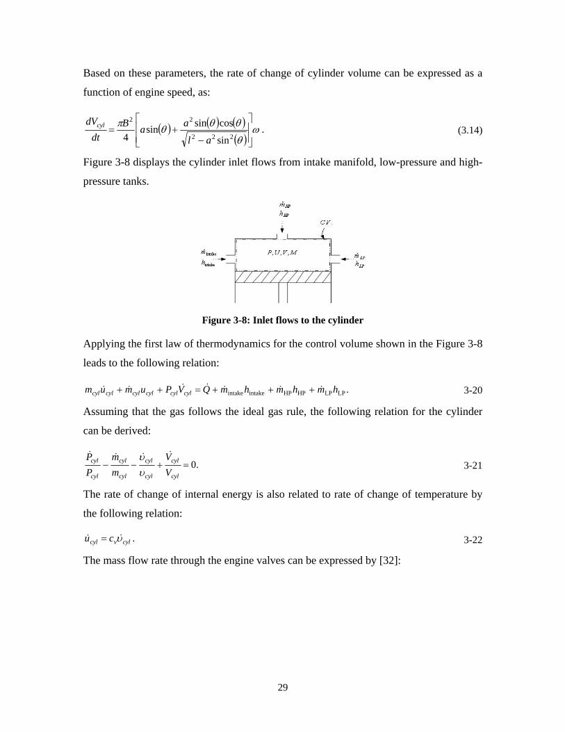
Figure 3-8 displays the cylinder inlet flows from intake manifold, low-pressure and high-
pressure tanks.
Figure 3-8: Inlet flows to the cylinder
Applying the first law of thermodynamics for the control volume shown in the Figure 3-8
leads to the following relation:
.LPLPHPHPintakeintake hmhmhmQVPumum cylcylcylcylcylcyl &&&&&&& +++=++ 3-20
Assuming that the gas follows the ideal gas rule, the following relation for the cylinder
can be derived:
.0=+−−cyl
cyl
cyl
cyl
cyl
cyl
cyl
cyl
VV
mm
PP &&&&
υυ
3-21
The rate of change of internal energy is also related to rate of change of temperature by
the following relation:
.cylvcyl cu υ&& = 3-22
The mass flow rate through the engine valves can be expressed by [32]:
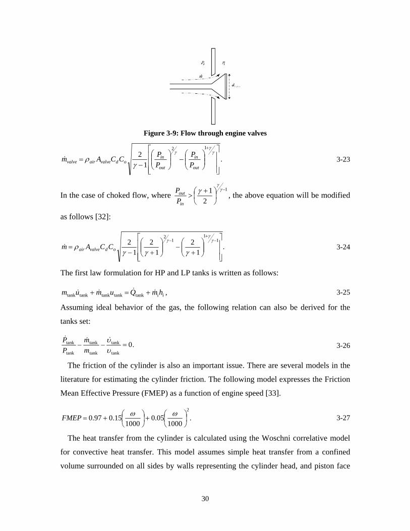
30
Figure 3-9: Flow through engine valves
.1
212
⎥⎥⎥
⎦
⎤
⎢⎢⎢
⎣
⎡
⎟⎟⎠
⎞⎜⎜⎝
⎛−⎟⎟
⎠
⎞⎜⎜⎝
⎛−
=
+γ
γγ
γρ
out
in
out
inodvalveairvalve P
PPPCCAm& 3-23
In the case of choked flow, where 1
21 −⎟⎠⎞
⎜⎝⎛ +
>γ
γγ
in
out
PP , the above equation will be modified
as follows [32]:
.1
21
21
2 11
12
⎥⎥⎥
⎦
⎤
⎢⎢⎢
⎣
⎡
⎟⎟⎠
⎞⎜⎜⎝
⎛+
−⎟⎟⎠
⎞⎜⎜⎝
⎛+−
=−
+− γ
γγ
γγγρ odvalveair CCAm& 3-24
The first law formulation for HP and LP tanks is written as follows:
,itanktanktanktanktank ihmQumum &&&& +=+ 3-25
Assuming ideal behavior of the gas, the following relation can also be derived for the
tanks set:
.0tank
tank
tank
tank
tank
tank =−−υυ&&&
mm
PP 3-26
The friction of the cylinder is also an important issue. There are several models in the
literature for estimating the cylinder friction. The following model expresses the Friction
Mean Effective Pressure (FMEP) as a function of engine speed [33].
.1000
05.01000
15.097.02
⎟⎠⎞
⎜⎝⎛+⎟
⎠⎞
⎜⎝⎛+=
ωωFMEP 3-27
The heat transfer from the cylinder is calculated using the Woschni correlative model
for convective heat transfer. This model assumes simple heat transfer from a confined
volume surrounded on all sides by walls representing the cylinder head, and piston face
31
areas exposed to the combustion chamber [33]. The heat transfer coefficient of Woschni
model is:
.26.3 8.055.08.02.0gascylcyl vPB −−= υh 3-28
In the above equation, gasv is the gas mean speed and is estimated by the following
relation [34]:
,28.2 pgas vv = 3-29
where ωavp 4= . Based on the Woschni model, heat transfer to the cylinder is expressed
as:
( ) ,cylccylcyl AQ υυ −= h& 3-30
where cυ is coolant temperature and cylA is the cylinder exposed area which is a function
of the crank angle based on:
( ) ( ) ( ) ( )( ) .sin/cos1/2
5.022 ⎟⎠⎞⎜
⎝⎛ −+−++= θθππ alalBaBAcyl 3-31
For the sake of simplicity, heat flux from the tanks surfaces is modeled by the following
relations:
( ),0 LPLPLPQ υυ −= h& 3-32
( ),0 HPHPHPQ υυ −= h& 3-33
where oυ is environment temperature. As discussed previously, to increase the efficiency
of compression braking LP tank should be cooled down but the HP tank should be
insulated. Since there is no specific design for both of the tanks, LPh is considered to be
much larger than HPh .
The above differential equations could be coupled with vehicle dynamic equations
through the following relation:
( )( ) .sgn ., vFVVFMEPPP BrakingTraccylcylatmcyl =+− && 3-34
Vehicle velocity, which is related to the engine speed by:
.1 ωrG
v = 3-35
32
The vehicle dynamic equation is also written as follows:
( ) .sin21 2
, vMfgMgMvACF vehiclervehiclevehicledairbrakingtrac &=−−− θρ 3-36
Equations (3-14) to (3-36) comprise a system of nonlinear differential equations which
should be solved together.
3.6 Simulation of Mathematical and GT-POWER Models
GT-POWER is a simulation program which is widely used by major vehicle
manufacturers and engine developers. It can be used for engine and powertrain analysis.
This software is based on 1-D simulation of gas dynamics and has the ability to model
and analyze heat transfer, combustion, and vibration. In this section, the simulation
results of the mathematical model described in Section 3.5 and GT-POWER model for
both single-tank and double-tank regenerative braking system are presented and
compared. A vehicle quarter model with the specifications shown in Table 3-2
decelerated from 80 [km/hr] to a complete stop utilizing a single-storage regenerative
braking system.
Table 3-2: Vehicle quarter model specifications 1 Vehicle Mass 1800/4 [kg] Initial Velocity 80 [km/hr] Final Velocity 0 [km/hr] Engine Displacement 450 [cc] Compression Ratio 8.5 HP Tank Volume 10 [l] LP Tank Volume 1 [l]
Table 3-3 lists intake and charging fixed valve timing with respect to TDC used in both
GT-POWER and mathematical model.
Table 3-3: Single tank system valve timing Opening Degree Closing Degree Intake Valve 20 160 Charging Valve 270 350
1 More simulation parameters may be found in Appendix E
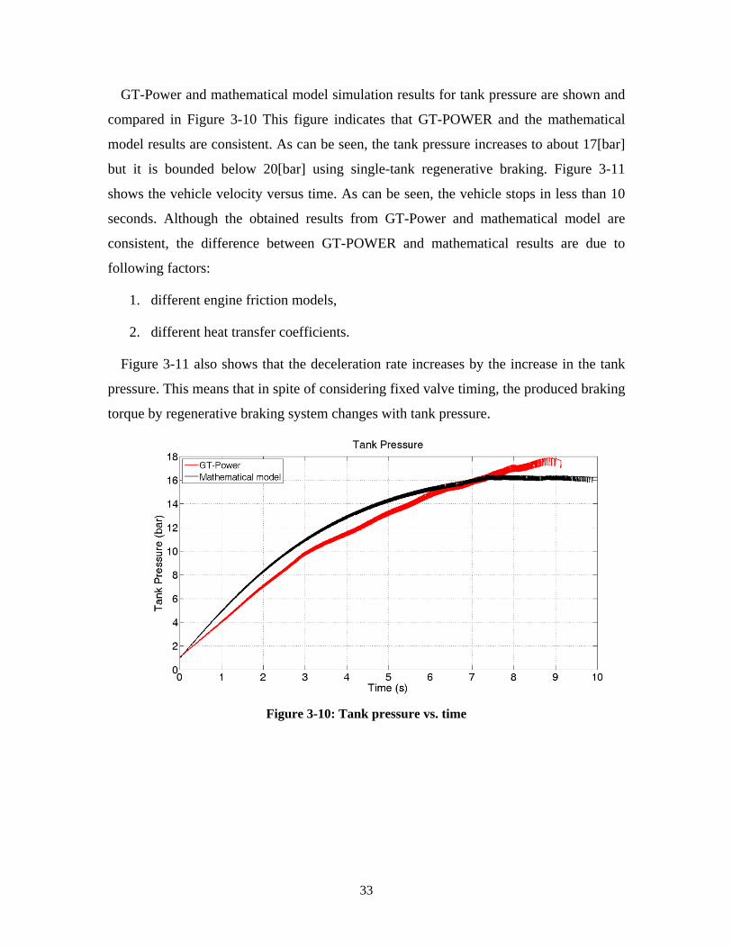
33
GT-Power and mathematical model simulation results for tank pressure are shown and
compared in Figure 3-10 This figure indicates that GT-POWER and the mathematical
model results are consistent. As can be seen, the tank pressure increases to about 17[bar]
but it is bounded below 20[bar] using single-tank regenerative braking. Figure 3-11
shows the vehicle velocity versus time. As can be seen, the vehicle stops in less than 10
seconds. Although the obtained results from GT-Power and mathematical model are
consistent, the difference between GT-POWER and mathematical results are due to
following factors:
1. different engine friction models,
2. different heat transfer coefficients.
Figure 3-11 also shows that the deceleration rate increases by the increase in the tank
pressure. This means that in spite of considering fixed valve timing, the produced braking
torque by regenerative braking system changes with tank pressure.
Figure 3-10: Tank pressure vs. time
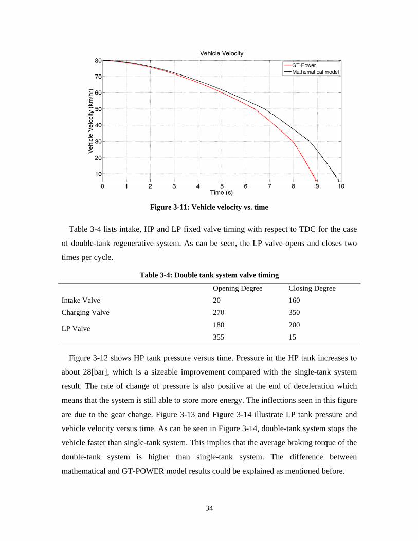
34
Figure 3-11: Vehicle velocity vs. time
Table 3-4 lists intake, HP and LP fixed valve timing with respect to TDC for the case
of double-tank regenerative system. As can be seen, the LP valve opens and closes two
times per cycle.
Table 3-4: Double tank system valve timing Opening Degree Closing Degree Intake Valve 20 160 Charging Valve 270 350
LP Valve 180 200 355 15
Figure 3-12 shows HP tank pressure versus time. Pressure in the HP tank increases to
about 28[bar], which is a sizeable improvement compared with the single-tank system
result. The rate of change of pressure is also positive at the end of deceleration which
means that the system is still able to store more energy. The inflections seen in this figure
are due to the gear change. Figure 3-13 and Figure 3-14 illustrate LP tank pressure and
vehicle velocity versus time. As can be seen in Figure 3-14, double-tank system stops the
vehicle faster than single-tank system. This implies that the average braking torque of the
double-tank system is higher than single-tank system. The difference between
mathematical and GT-POWER model results could be explained as mentioned before.
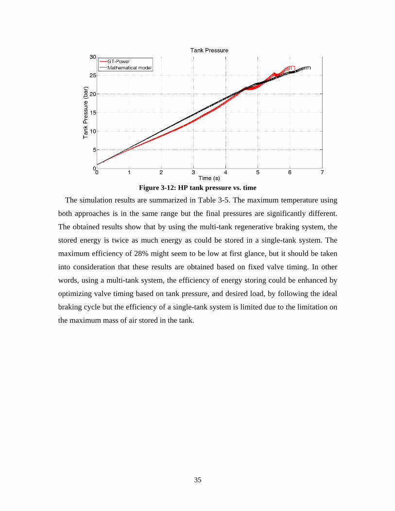
35
Figure 3-12: HP tank pressure vs. time
The simulation results are summarized in Table 3-5. The maximum temperature using
both approaches is in the same range but the final pressures are significantly different.
The obtained results show that by using the multi-tank regenerative braking system, the
stored energy is twice as much energy as could be stored in a single-tank system. The
maximum efficiency of 28% might seem to be low at first glance, but it should be taken
into consideration that these results are obtained based on fixed valve timing. In other
words, using a multi-tank system, the efficiency of energy storing could be enhanced by
optimizing valve timing based on tank pressure, and desired load, by following the ideal
braking cycle but the efficiency of a single-tank system is limited due to the limitation on
the maximum mass of air stored in the tank.
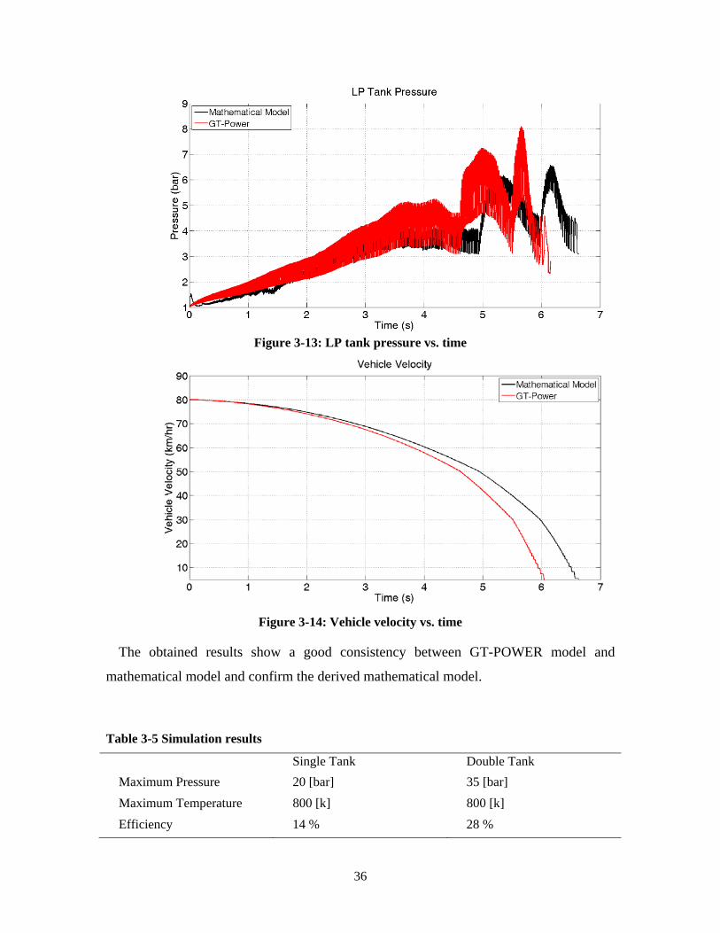
36
Figure 3-13: LP tank pressure vs. time
Figure 3-14: Vehicle velocity vs. time
The obtained results show a good consistency between GT-POWER model and
mathematical model and confirm the derived mathematical model.
Table 3-5 Simulation results
Single Tank Double Tank Maximum Pressure 20 [bar] 35 [bar] Maximum Temperature 800 [k] 800 [k] Efficiency 14 % 28 %
37
3.7 Summary
In this chapter a new compression strategy was introduced for air hybrid engines. The
theoretical results showed the advantage of the proposed strategy over the conventional
single-tank system. The proposed compression algorithm can be utilized in an air hybrid
vehicle to increase the efficiency of energy recovery by the compression braking system.
Compared to the double-stage regenerative braking, the double-tank system doubles the
air flow rate because only one cylinder is needed to implement the proposed concept and
thus, all the cylinders can be connected directly to the main tank. The proposed
compression algorithm can be applied not only in air hybrid vehicle compression braking
system, but also in any other applications where higher pressure with higher air mass
flow rate is demanded such as typical reciprocating compressors. Double-tank
compressors are expected to have the same working pressure and outlet flow rate as
double-stage compressors, but with a weight of almost half of a double-stage one. The
following chapter presents the experimental results of implementing the double-tank
regenerative system.
38
Chapter 4 Experimental Analysis
To test the proposed double-tank compression technique and compare it with the single-
tank technique in practice, an experimental setup has been designed and built as shown in
Figure 4-1 and Figure 4-2. This setup enables the testing of two modes of operation: AM
and CB. In the setup, a single cylinder engine has been turned into an air hybrid engine
by replacing the cylinder head with a new one that connects the engine to two air tanks.
Figure 4-1 shows the schematic of the system layout. A servo DC motor is connected to a
large flywheel through an electromagnetic clutch and an electromagnetic brake. The
motor shaft is connected to the engine shaft by a timing pulleys set with the ratio of
60/28. The engine angular rotation is measured by an incremental encoder mounted on
the engine shaft. The encoder’s signal defines the accurate angular position of the crank
shaft w.r.t. TDC. The experimental set-up is comprised of the following components:
1. A single cylinder engine
2. Electromagnetic clutch and brake
3. Flywheel
4. Servo motor and drive
5. Timing pulleys
6. Pressure sensors
7. Thermocouples
8. Small and large tanks
9. Solenoid valves
10. Beckhoff PLC controller
11. Encoder
12. Couplings and universal joint
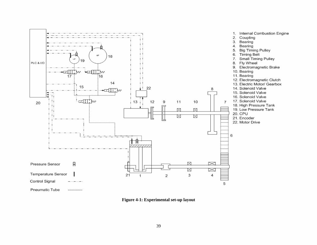
39
Figure 4-1: Experimental set-up layout
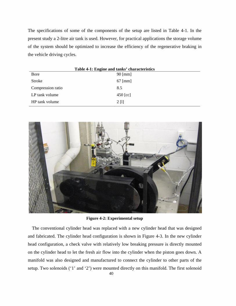
40
The specifications of some of the components of the setup are listed in Table 4-1. In the
present study a 2-litre air tank is used. However, for practical applications the storage volume
of the system should be optimized to increase the efficiency of the regenerative braking in
the vehicle driving cycles.
Table 4-1: Engine and tanks’ characteristics Bore 90 [mm] Stroke 67 [mm] Compression ratio 8.5 LP tank volume 450 [cc] HP tank volume 2 [l]
Figure 4-2: Experimental setup
The conventional cylinder head was replaced with a new cylinder head that was designed
and fabricated. The cylinder head configuration is shown in Figure 4-3. In the new cylinder
head configuration, a check valve with relatively low breaking pressure is directly mounted
on the cylinder head to let the fresh air flow into the cylinder when the piston goes down. A
manifold was also designed and manufactured to connect the cylinder to other parts of the
setup. Two solenoids (‘1’ and ‘2’) were mounted directly on this manifold. The first solenoid
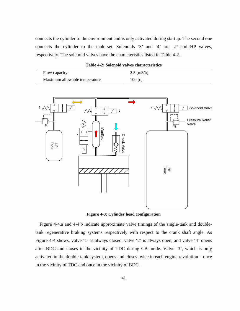
41
connects the cylinder to the environment and is only activated during startup. The second one
connects the cylinder to the tank set. Solenoids ‘3’ and ‘4’ are LP and HP valves,
respectively. The solenoid valves have the characteristics listed in Table 4-2.
Table 4-2: Solenoid valves characteristics
Flow capacity 2.5 [m3/h] Maximum allowable temperature 100 [c]
Figure 4-3: Cylinder head configuration
Figure 4-4.a and 4-4.b indicate approximate valve timings of the single-tank and double-
tank regenerative braking systems respectively with respect to the crank shaft angle. As
Figure 4-4 shows, valve ‘1’ is always closed, valve ‘2’ is always open, and valve ‘4’ opens
after BDC and closes in the vicinity of TDC during CB mode. Valve ‘3’, which is only
activated in the double-tank system, opens and closes twice in each engine revolution – once
in the vicinity of TDC and once in the vicinity of BDC.
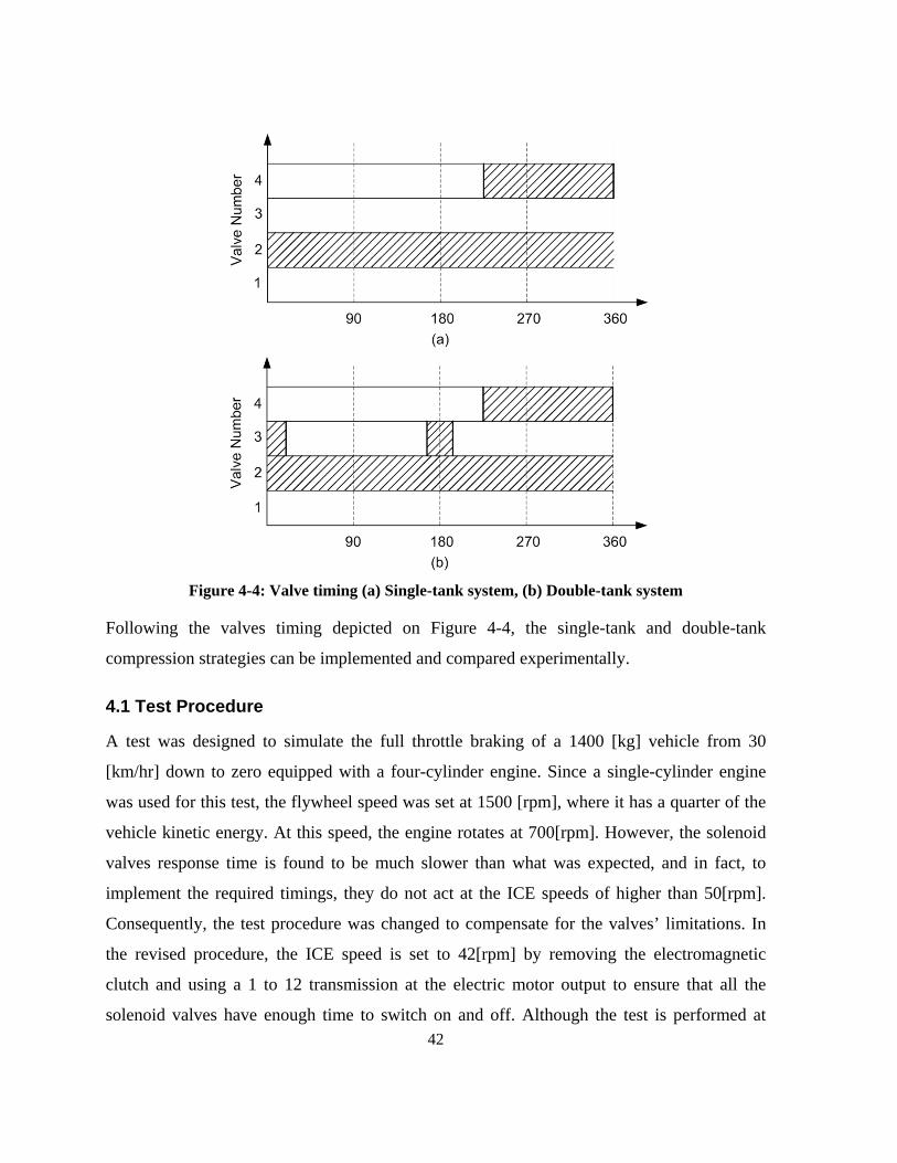
42
Figure 4-4: Valve timing (a) Single-tank system, (b) Double-tank system
Following the valves timing depicted on Figure 4-4, the single-tank and double-tank
compression strategies can be implemented and compared experimentally.
4.1 Test Procedure
A test was designed to simulate the full throttle braking of a 1400 [kg] vehicle from 30
[km/hr] down to zero equipped with a four-cylinder engine. Since a single-cylinder engine
was used for this test, the flywheel speed was set at 1500 [rpm], where it has a quarter of the
vehicle kinetic energy. At this speed, the engine rotates at 700[rpm]. However, the solenoid
valves response time is found to be much slower than what was expected, and in fact, to
implement the required timings, they do not act at the ICE speeds of higher than 50[rpm].
Consequently, the test procedure was changed to compensate for the valves’ limitations. In
the revised procedure, the ICE speed is set to 42[rpm] by removing the electromagnetic
clutch and using a 1 to 12 transmission at the electric motor output to ensure that all the
solenoid valves have enough time to switch on and off. Although the test is performed at
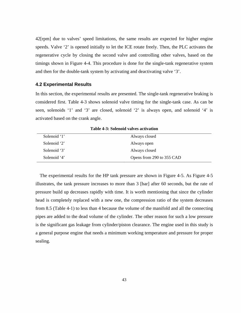
43
42[rpm] due to valves’ speed limitations, the same results are expected for higher engine
speeds. Valve ‘2’ is opened initially to let the ICE rotate freely. Then, the PLC activates the
regenerative cycle by closing the second valve and controlling other valves, based on the
timings shown in Figure 4-4. This procedure is done for the single-tank regenerative system
and then for the double-tank system by activating and deactivating valve ‘3’.
4.2 Experimental Results
In this section, the experimental results are presented. The single-tank regenerative braking is
considered first. Table 4-3 shows solenoid valve timing for the single-tank case. As can be
seen, solenoids ‘1’ and ‘3’ are closed, solenoid ‘2’ is always open, and solenoid ‘4’ is
activated based on the crank angle.
Table 4-3: Solenoid valves activation
Solenoid ‘1’ Always closed Solenoid ‘2’ Always open Solenoid ‘3’ Always closed Solenoid ‘4’ Opens from 290 to 355 CAD
The experimental results for the HP tank pressure are shown in Figure 4-5. As Figure 4-5
illustrates, the tank pressure increases to more than 3 [bar] after 60 seconds, but the rate of
pressure build up decreases rapidly with time. It is worth mentioning that since the cylinder
head is completely replaced with a new one, the compression ratio of the system decreases
from 8.5 (Table 4-1) to less than 4 because the volume of the manifold and all the connecting
pipes are added to the dead volume of the cylinder. The other reason for such a low pressure
is the significant gas leakage from cylinder/piston clearance. The engine used in this study is
a general purpose engine that needs a minimum working temperature and pressure for proper
sealing.
44
Figure 4-5: HP tank pressure obtained from experiment
The double-tank regenerative braking is tested in the next experiment. Here, the solenoid
valves are activated based on Table 4-4. Solenoid ‘3’ is switched on and off twice during
each cycle, once in the vicinity of TDC and once in the vicinity of BTC. The results are
shown in Figure 4-6 and Figure 4-7.
Table 4-4: Solenoid valves activation Solenoid ‘1’ Always closed
Solenoid ‘2’ Always open
Solenoid ‘3’ Opens from 170 to 190 and from 5 to 25 CAD
Solenoid ‘4’ Opens from 290 to 355 CAD
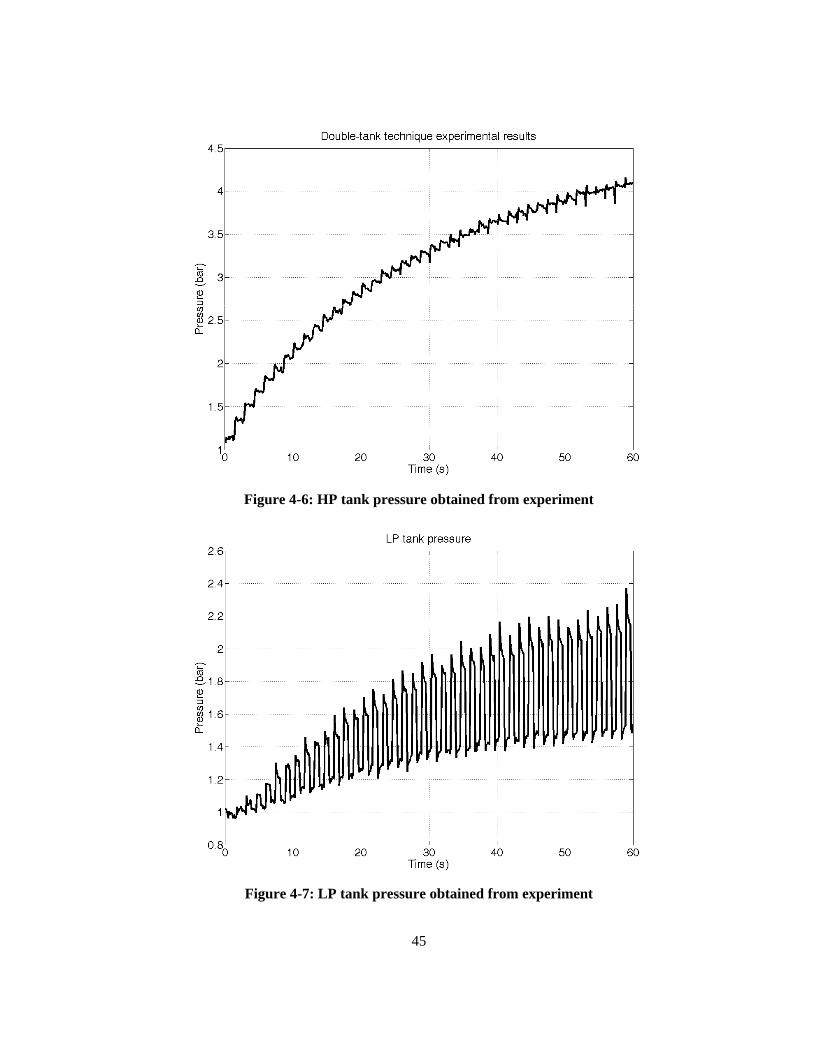
45
Figure 4-6: HP tank pressure obtained from experiment
Figure 4-7: LP tank pressure obtained from experiment
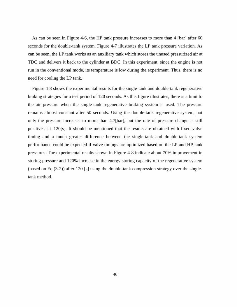
46
As can be seen in Figure 4-6, the HP tank pressure increases to more than 4 [bar] after 60
seconds for the double-tank system. Figure 4-7 illustrates the LP tank pressure variation. As
can be seen, the LP tank works as an auxiliary tank which stores the unused pressurized air at
TDC and delivers it back to the cylinder at BDC. In this experiment, since the engine is not
run in the conventional mode, its temperature is low during the experiment. Thus, there is no
need for cooling the LP tank.
Figure 4-8 shows the experimental results for the single-tank and double-tank regenerative
braking strategies for a test period of 120 seconds. As this figure illustrates, there is a limit to
the air pressure when the single-tank regenerative braking system is used. The pressure
remains almost constant after 50 seconds. Using the double-tank regenerative system, not
only the pressure increases to more than 4.7[bar], but the rate of pressure change is still
positive at t=120[s]. It should be mentioned that the results are obtained with fixed valve
timing and a much greater difference between the single-tank and double-tank system
performance could be expected if valve timings are optimized based on the LP and HP tank
pressures. The experimental results shown in Figure 4-8 indicate about 70% improvement in
storing pressure and 120% increase in the energy storing capacity of the regenerative system
(based on Eq.(3-2)) after 120 [s] using the double-tank compression strategy over the single-
tank method.
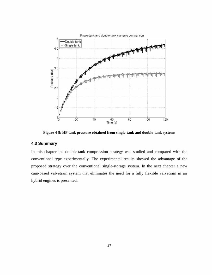
47
Figure 4-8: HP tank pressure obtained from single-tank and double-tank systems
4.3 Summary
In this chapter the double-tank compression strategy was studied and compared with the
conventional type experimentally. The experimental results showed the advantage of the
proposed strategy over the conventional single-storage system. In the next chapter a new
cam-based valvetrain system that eliminates the need for a fully flexible valvetrain in air
hybrid engines is presented.
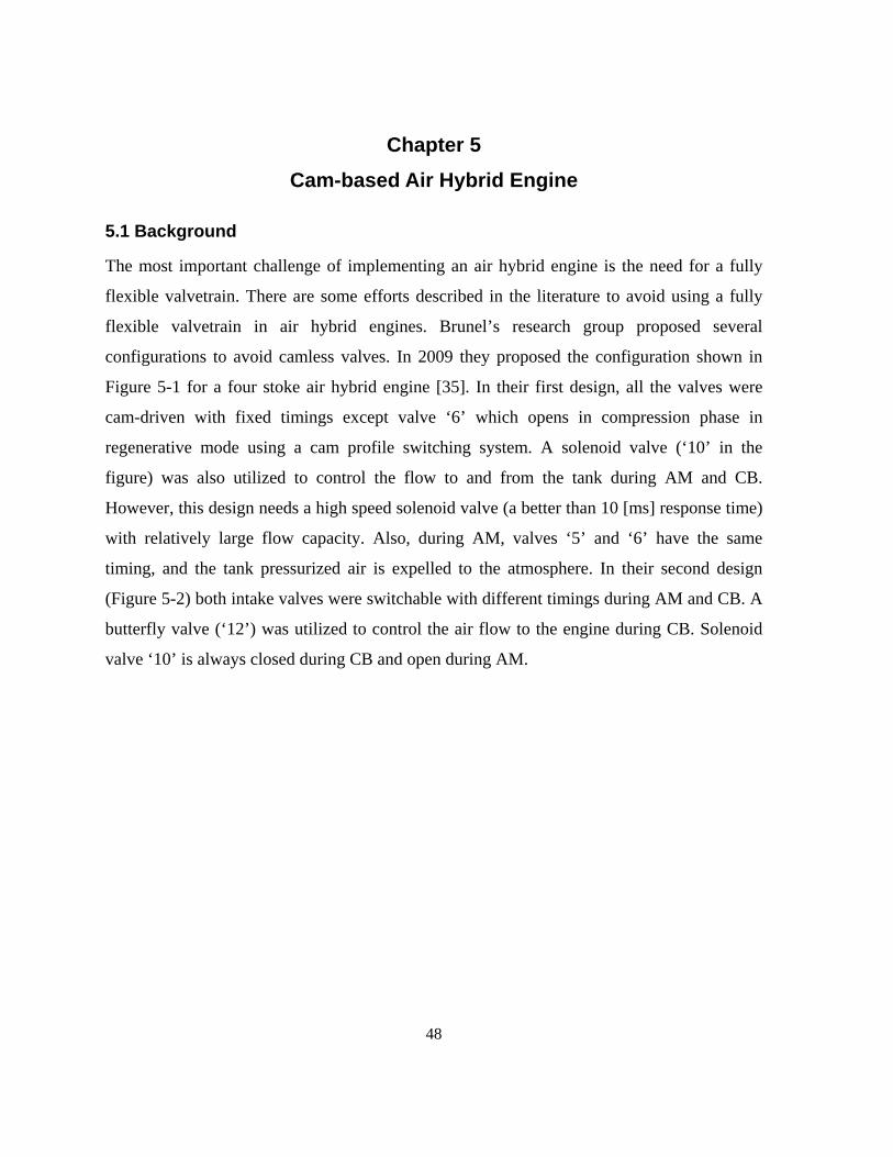
48
Chapter 5 Cam-based Air Hybrid Engine
5.1 Background
The most important challenge of implementing an air hybrid engine is the need for a fully
flexible valvetrain. There are some efforts described in the literature to avoid using a fully
flexible valvetrain in air hybrid engines. Brunel’s research group proposed several
configurations to avoid camless valves. In 2009 they proposed the configuration shown in
Figure 5-1 for a four stoke air hybrid engine [35]. In their first design, all the valves were
cam-driven with fixed timings except valve ‘6’ which opens in compression phase in
regenerative mode using a cam profile switching system. A solenoid valve (‘10’ in the
figure) was also utilized to control the flow to and from the tank during AM and CB.
However, this design needs a high speed solenoid valve (a better than 10 [ms] response time)
with relatively large flow capacity. Also, during AM, valves ‘5’ and ‘6’ have the same
timing, and the tank pressurized air is expelled to the atmosphere. In their second design
(Figure 5-2) both intake valves were switchable with different timings during AM and CB. A
butterfly valve (‘12’) was utilized to control the air flow to the engine during CB. Solenoid
valve ‘10’ is always closed during CB and open during AM.
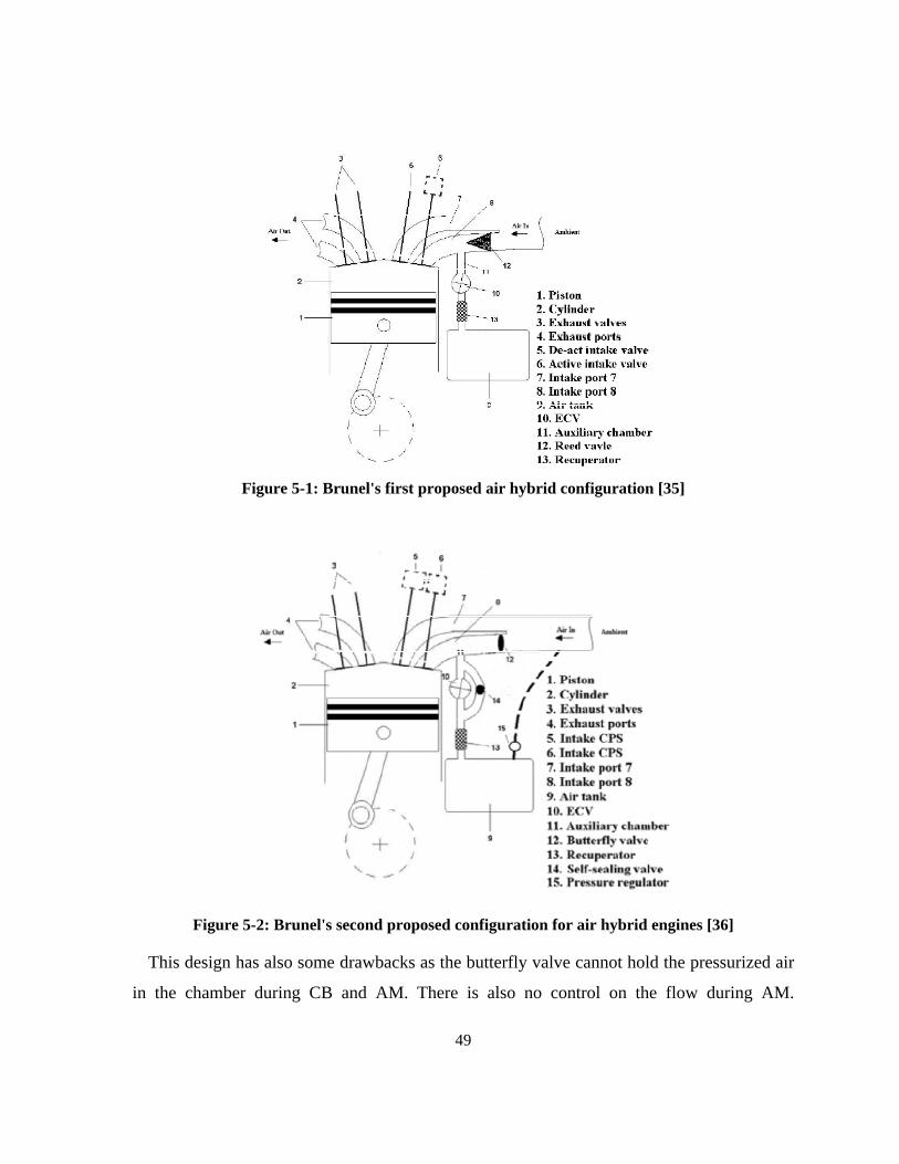
49
Figure 5-1: Brunel's first proposed air hybrid configuration [35]
Figure 5-2: Brunel's second proposed configuration for air hybrid engines [36]
This design has also some drawbacks as the butterfly valve cannot hold the pressurized air
in the chamber during CB and AM. There is also no control on the flow during AM.
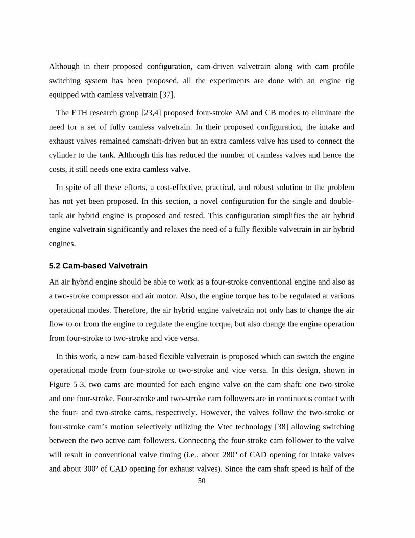
50
Although in their proposed configuration, cam-driven valvetrain along with cam profile
switching system has been proposed, all the experiments are done with an engine rig
equipped with camless valvetrain [37].
The ETH research group [23,4] proposed four-stroke AM and CB modes to eliminate the
need for a set of fully camless valvetrain. In their proposed configuration, the intake and
exhaust valves remained camshaft-driven but an extra camless valve has used to connect the
cylinder to the tank. Although this has reduced the number of camless valves and hence the
costs, it still needs one extra camless valve.
In spite of all these efforts, a cost-effective, practical, and robust solution to the problem
has not yet been proposed. In this section, a novel configuration for the single and double-
tank air hybrid engine is proposed and tested. This configuration simplifies the air hybrid
engine valvetrain significantly and relaxes the need of a fully flexible valvetrain in air hybrid
engines.
5.2 Cam-based Valvetrain
An air hybrid engine should be able to work as a four-stroke conventional engine and also as
a two-stroke compressor and air motor. Also, the engine torque has to be regulated at various
operational modes. Therefore, the air hybrid engine valvetrain not only has to change the air
flow to or from the engine to regulate the engine torque, but also change the engine operation
from four-stroke to two-stroke and vice versa.
In this work, a new cam-based flexible valvetrain is proposed which can switch the engine
operational mode from four-stroke to two-stroke and vice versa. In this design, shown in
Figure 5-3, two cams are mounted for each engine valve on the cam shaft: one two-stroke
and one four-stroke. Four-stroke and two-stroke cam followers are in continuous contact with
the four- and two-stroke cams, respectively. However, the valves follow the two-stroke or
four-stroke cam’s motion selectively utilizing the Vtec technology [38] allowing switching
between the two active cam followers. Connecting the four-stroke cam follower to the valve
will result in conventional valve timing (i.e., about 280º of CAD opening for intake valves
and about 300º of CAD opening for exhaust valves). Since the cam shaft speed is half of the
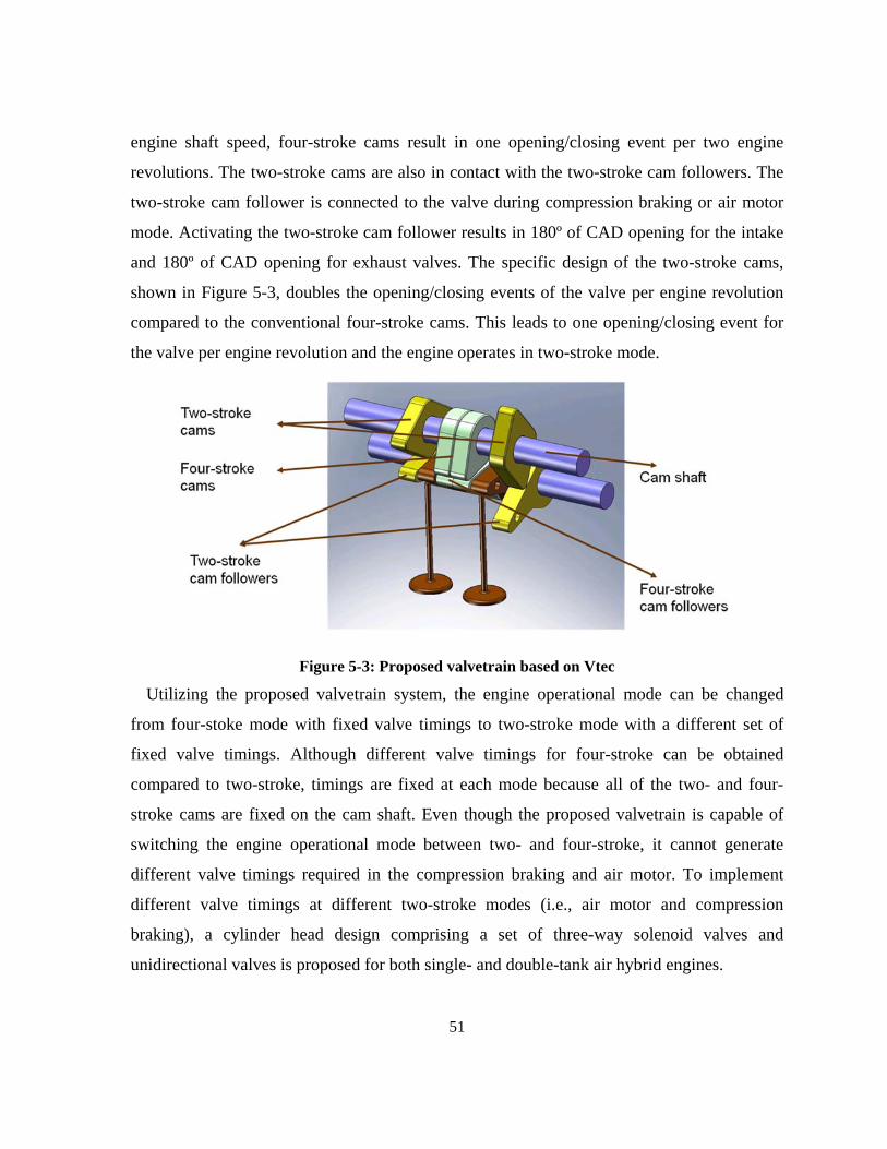
51
engine shaft speed, four-stroke cams result in one opening/closing event per two engine
revolutions. The two-stroke cams are also in contact with the two-stroke cam followers. The
two-stroke cam follower is connected to the valve during compression braking or air motor
mode. Activating the two-stroke cam follower results in 180º of CAD opening for the intake
and 180º of CAD opening for exhaust valves. The specific design of the two-stroke cams,
shown in Figure 5-3, doubles the opening/closing events of the valve per engine revolution
compared to the conventional four-stroke cams. This leads to one opening/closing event for
the valve per engine revolution and the engine operates in two-stroke mode.
Figure 5-3: Proposed valvetrain based on Vtec
Utilizing the proposed valvetrain system, the engine operational mode can be changed
from four-stoke mode with fixed valve timings to two-stroke mode with a different set of
fixed valve timings. Although different valve timings for four-stroke can be obtained
compared to two-stroke, timings are fixed at each mode because all of the two- and four-
stroke cams are fixed on the cam shaft. Even though the proposed valvetrain is capable of
switching the engine operational mode between two- and four-stroke, it cannot generate
different valve timings required in the compression braking and air motor. To implement
different valve timings at different two-stroke modes (i.e., air motor and compression
braking), a cylinder head design comprising a set of three-way solenoid valves and
unidirectional valves is proposed for both single- and double-tank air hybrid engines.
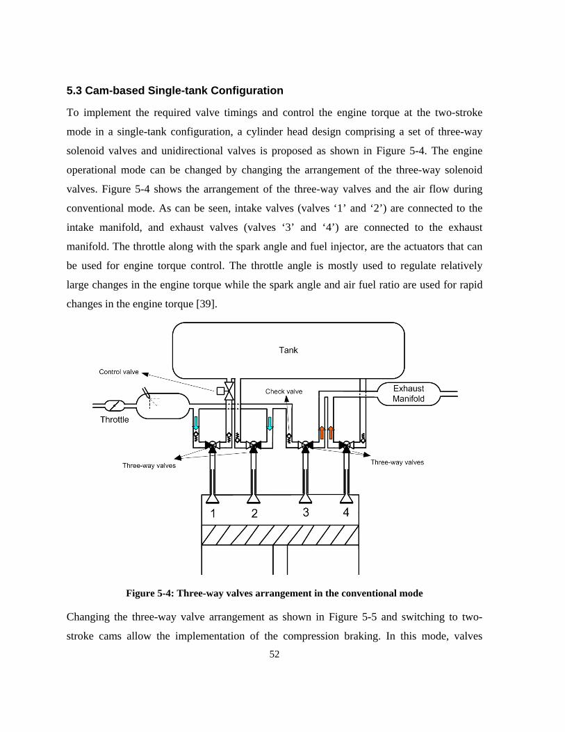
52
5.3 Cam-based Single-tank Configuration
To implement the required valve timings and control the engine torque at the two-stroke
mode in a single-tank configuration, a cylinder head design comprising a set of three-way
solenoid valves and unidirectional valves is proposed as shown in Figure 5-4. The engine
operational mode can be changed by changing the arrangement of the three-way solenoid
valves. Figure 5-4 shows the arrangement of the three-way valves and the air flow during
conventional mode. As can be seen, intake valves (valves ‘1’ and ‘2’) are connected to the
intake manifold, and exhaust valves (valves ‘3’ and ‘4’) are connected to the exhaust
manifold. The throttle along with the spark angle and fuel injector, are the actuators that can
be used for engine torque control. The throttle angle is mostly used to regulate relatively
large changes in the engine torque while the spark angle and air fuel ratio are used for rapid
changes in the engine torque [39].
Figure 5-4: Three-way valves arrangement in the conventional mode
Changing the three-way valve arrangement as shown in Figure 5-5 and switching to two-
stroke cams allow the implementation of the compression braking. In this mode, valves
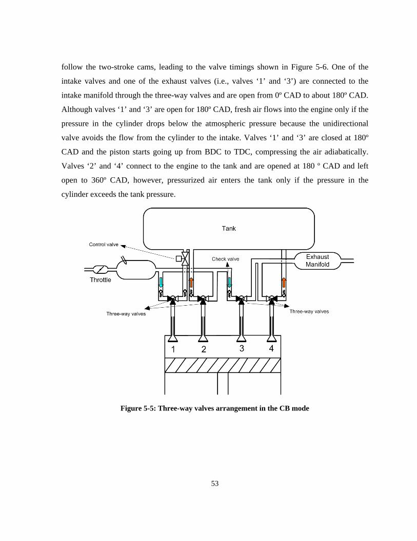
53
follow the two-stroke cams, leading to the valve timings shown in Figure 5-6. One of the
intake valves and one of the exhaust valves (i.e., valves ‘1’ and ‘3’) are connected to the
intake manifold through the three-way valves and are open from 0º CAD to about 180º CAD.
Although valves ‘1’ and ‘3’ are open for 180º CAD, fresh air flows into the engine only if the
pressure in the cylinder drops below the atmospheric pressure because the unidirectional
valve avoids the flow from the cylinder to the intake. Valves ‘1’ and ‘3’ are closed at 180º
CAD and the piston starts going up from BDC to TDC, compressing the air adiabatically.
Valves ‘2’ and ‘4’ connect to the engine to the tank and are opened at 180 º CAD and left
open to 360º CAD, however, pressurized air enters the tank only if the pressure in the
cylinder exceeds the tank pressure.
Figure 5-5: Three-way valves arrangement in the CB mode
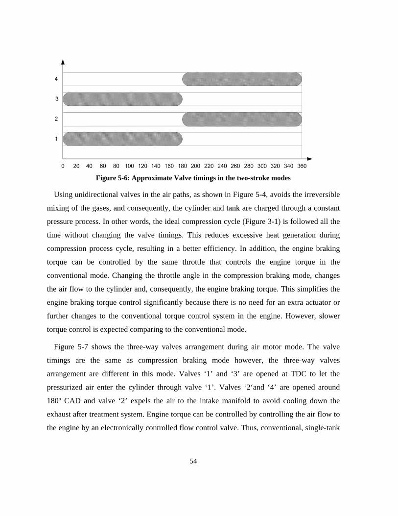
54
Figure 5-6: Approximate Valve timings in the two-stroke modes
Using unidirectional valves in the air paths, as shown in Figure 5-4, avoids the irreversible
mixing of the gases, and consequently, the cylinder and tank are charged through a constant
pressure process. In other words, the ideal compression cycle (Figure 3-1) is followed all the
time without changing the valve timings. This reduces excessive heat generation during
compression process cycle, resulting in a better efficiency. In addition, the engine braking
torque can be controlled by the same throttle that controls the engine torque in the
conventional mode. Changing the throttle angle in the compression braking mode, changes
the air flow to the cylinder and, consequently, the engine braking torque. This simplifies the
engine braking torque control significantly because there is no need for an extra actuator or
further changes to the conventional torque control system in the engine. However, slower
torque control is expected comparing to the conventional mode.
Figure 5-7 shows the three-way valves arrangement during air motor mode. The valve
timings are the same as compression braking mode however, the three-way valves
arrangement are different in this mode. Valves ‘1’ and ‘3’ are opened at TDC to let the
pressurized air enter the cylinder through valve ‘1’. Valves ‘2‘and ‘4’ are opened around
180º CAD and valve ‘2’ expels the air to the intake manifold to avoid cooling down the
exhaust after treatment system. Engine torque can be controlled by controlling the air flow to
the engine by an electronically controlled flow control valve. Thus, conventional, single-tank
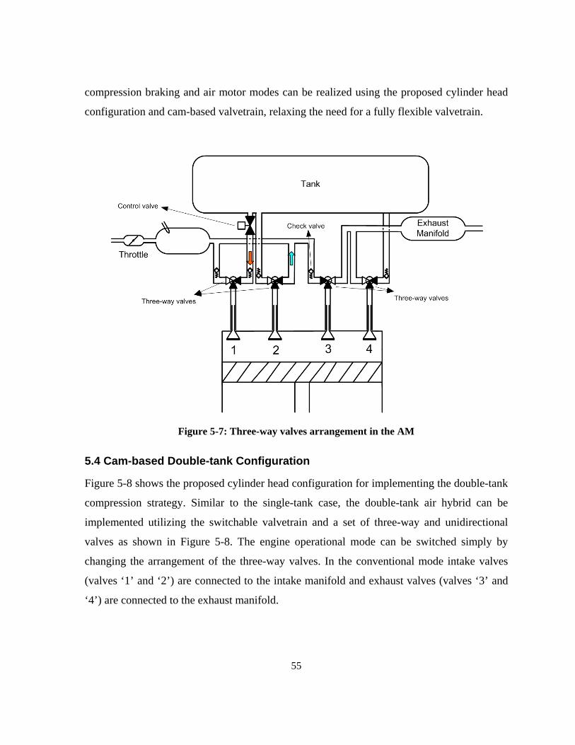
55
compression braking and air motor modes can be realized using the proposed cylinder head
configuration and cam-based valvetrain, relaxing the need for a fully flexible valvetrain.
Figure 5-7: Three-way valves arrangement in the AM
5.4 Cam-based Double-tank Configuration
Figure 5-8 shows the proposed cylinder head configuration for implementing the double-tank
compression strategy. Similar to the single-tank case, the double-tank air hybrid can be
implemented utilizing the switchable valvetrain and a set of three-way and unidirectional
valves as shown in Figure 5-8. The engine operational mode can be switched simply by
changing the arrangement of the three-way valves. In the conventional mode intake valves
(valves ‘1’ and ‘2’) are connected to the intake manifold and exhaust valves (valves ‘3’ and
‘4’) are connected to the exhaust manifold.
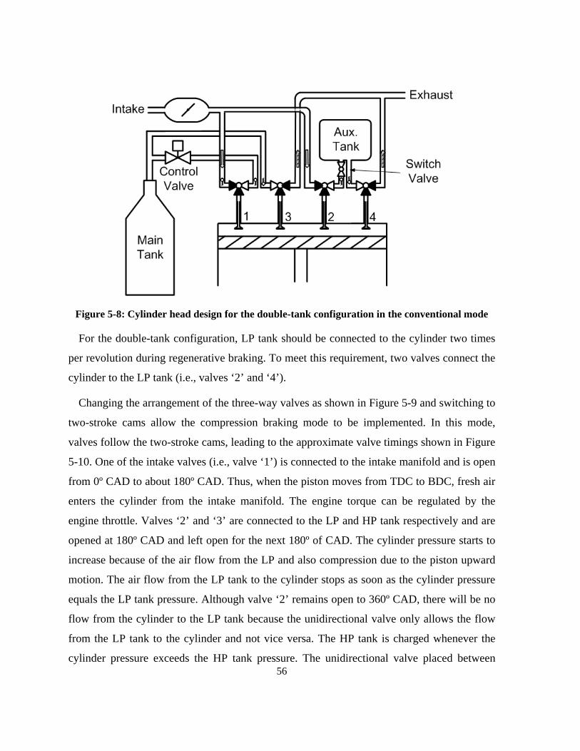
56
Figure 5-8: Cylinder head design for the double-tank configuration in the conventional mode
For the double-tank configuration, LP tank should be connected to the cylinder two times
per revolution during regenerative braking. To meet this requirement, two valves connect the
cylinder to the LP tank (i.e., valves ‘2’ and ‘4’).
Changing the arrangement of the three-way valves as shown in Figure 5-9 and switching to
two-stroke cams allow the compression braking mode to be implemented. In this mode,
valves follow the two-stroke cams, leading to the approximate valve timings shown in Figure
5-10. One of the intake valves (i.e., valve ‘1’) is connected to the intake manifold and is open
from 0º CAD to about 180º CAD. Thus, when the piston moves from TDC to BDC, fresh air
enters the cylinder from the intake manifold. The engine torque can be regulated by the
engine throttle. Valves ‘2’ and ‘3’ are connected to the LP and HP tank respectively and are
opened at 180º CAD and left open for the next 180º of CAD. The cylinder pressure starts to
increase because of the air flow from the LP and also compression due to the piston upward
motion. The air flow from the LP tank to the cylinder stops as soon as the cylinder pressure
equals the LP tank pressure. Although valve ‘2’ remains open to 360º CAD, there will be no
flow from the cylinder to the LP tank because the unidirectional valve only allows the flow
from the LP tank to the cylinder and not vice versa. The HP tank is charged whenever the
cylinder pressure exceeds the HP tank pressure. The unidirectional valve placed between
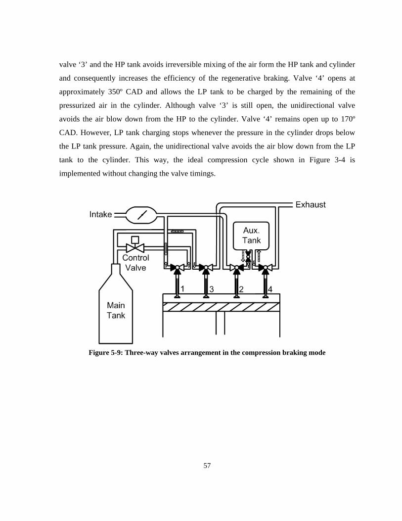
57
valve ‘3’ and the HP tank avoids irreversible mixing of the air form the HP tank and cylinder
and consequently increases the efficiency of the regenerative braking. Valve ‘4’ opens at
approximately 350º CAD and allows the LP tank to be charged by the remaining of the
pressurized air in the cylinder. Although valve ‘3’ is still open, the unidirectional valve
avoids the air blow down from the HP to the cylinder. Valve ‘4’ remains open up to 170º
CAD. However, LP tank charging stops whenever the pressure in the cylinder drops below
the LP tank pressure. Again, the unidirectional valve avoids the air blow down from the LP
tank to the cylinder. This way, the ideal compression cycle shown in Figure 3-4 is
implemented without changing the valve timings.
Figure 5-9: Three-way valves arrangement in the compression braking mode
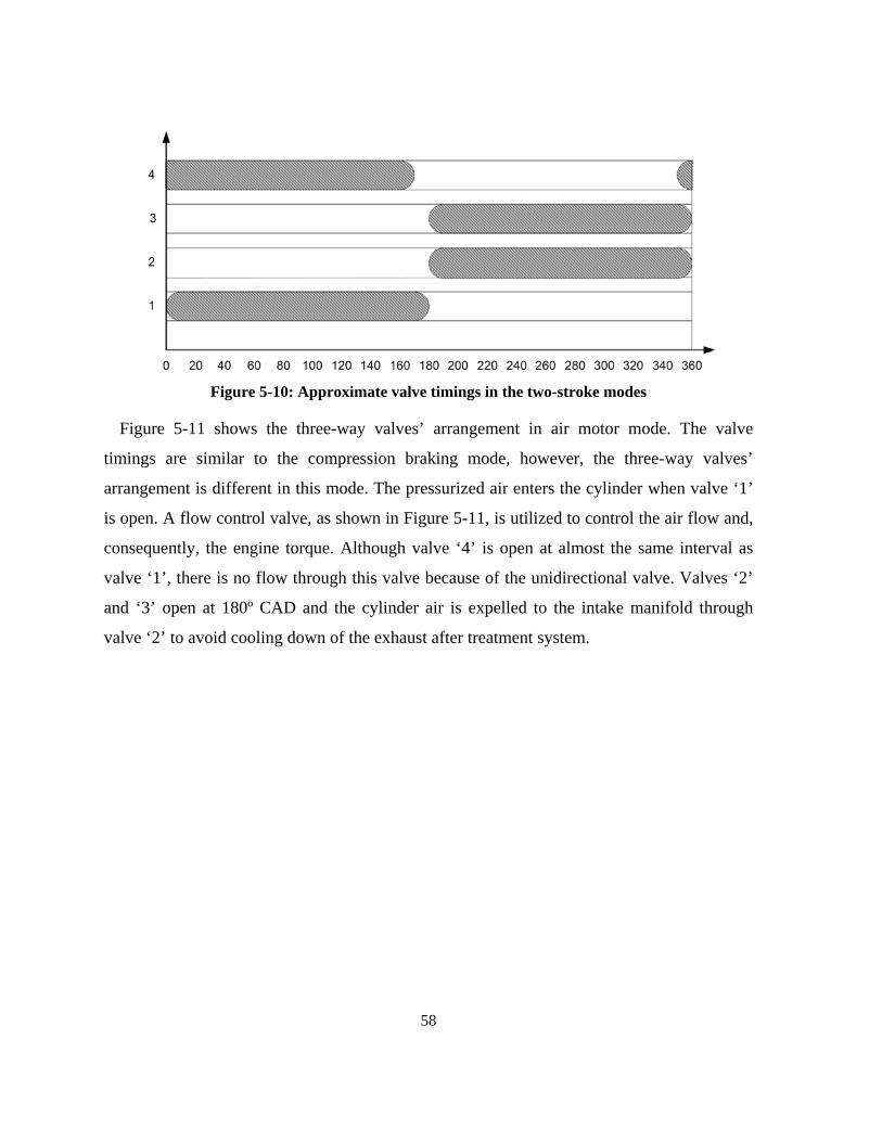
58
Figure 5-10: Approximate valve timings in the two-stroke modes
Figure 5-11 shows the three-way valves’ arrangement in air motor mode. The valve
timings are similar to the compression braking mode, however, the three-way valves’
arrangement is different in this mode. The pressurized air enters the cylinder when valve ‘1’
is open. A flow control valve, as shown in Figure 5-11, is utilized to control the air flow and,
consequently, the engine torque. Although valve ‘4’ is open at almost the same interval as
valve ‘1’, there is no flow through this valve because of the unidirectional valve. Valves ‘2’
and ‘3’ open at 180º CAD and the cylinder air is expelled to the intake manifold through
valve ‘2’ to avoid cooling down of the exhaust after treatment system.
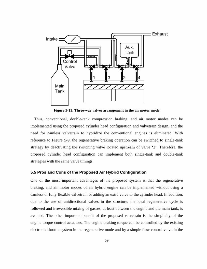
59
Figure 5-11: Three-way valves arrangement in the air motor mode
Thus, conventional, double-tank compression braking, and air motor modes can be
implemented using the proposed cylinder head configuration and valvetrain design, and the
need for camless valvetrain to hybridize the conventional engines is eliminated. With
reference to Figure 5-9, the regenerative braking operation can be switched to single-tank
strategy by deactivating the switching valve located upstream of valve ‘2’. Therefore, the
proposed cylinder head configuration can implement both single-tank and double-tank
strategies with the same valve timings.
5.5 Pros and Cons of the Proposed Air Hybrid Configuration
One of the most important advantages of the proposed system is that the regenerative
braking, and air motor modes of air hybrid engine can be implemented without using a
camless or fully flexible valvetrain or adding an extra valve to the cylinder head. In addition,
due to the use of unidirectional valves in the structure, the ideal regenerative cycle is
followed and irreversible mixing of gasses, at least between the engine and the main tank, is
avoided. The other important benefit of the proposed valvetrain is the simplicity of the
engine torque control actuators. The engine braking torque can be controlled by the existing
electronic throttle system in the regenerative mode and by a simple flow control valve in the
60
air motor mode, eliminating the need for a complete valve timing control. Furthermore, both
the single- and double-tank compression strategies can be implemented by the proposed
double-tank air hybrid engine configuration.
In spite of the above mentioned advantages, there might be some drawbacks associated
with the proposed cylinder head design which requires further studies. The configuration of
such an intake system and the use of three-way valves and check valves introduce resistance
to the air flow and hence results in poor engine performance. Although there is no need for
high speed three-way solenoid valves (as they just change the operational mode), they need
to have good resistance against high temperature as they are exposed to exhaust gas. In
addition, the compression ratio of the engine in regenerative mode could drop as the three-
way and check valves volumes are added to the cylinder volume.
5.6 Simulations
5.6.1 Regenerative Braking
To study the performance of the proposed cylinder head design in capturing the kinetic
energy of a vehicle, full throttle deceleration of a Ford 150 truck equipped with 5.4[L] V8
engine from 70 [km/hr] down to 10 [km/hr] is modeled in GT-Power. The valvetrain and
cylinder head design proposed in Sections 5.3 and 5.4 is utilized to implement the air hybrid
engine concept for both single- and double-tank systems. The vehicle and engine
specifications are tabulated in Table 5-1. It is noteworthy that all the three-way valves and
check valves flow characteristics and their related energy losses are considered in
GT_Power.
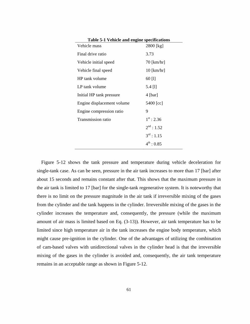
61
Table 5-1 Vehicle and engine specifications Vehicle mass 2800 [kg]
Final drive ratio 3.73
Vehicle initial speed 70 [km/hr]
Vehicle final speed 10 [km/hr]
HP tank volume 60 [l]
LP tank volume 5.4 [l]
Initial HP tank pressure 4 [bar]
Engine displacement volume 5400 [cc]
Engine compression ratio 9
Transmission ratio 1st : 2.36
2nd : 1.52
3rd : 1.15
4th : 0.85
Figure 5-12 shows the tank pressure and temperature during vehicle deceleration for
single-tank case. As can be seen, pressure in the air tank increases to more than 17 [bar] after
about 15 seconds and remains constant after that. This shows that the maximum pressure in
the air tank is limited to 17 [bar] for the single-tank regenerative system. It is noteworthy that
there is no limit on the pressure magnitude in the air tank if irreversible mixing of the gases
from the cylinder and the tank happens in the cylinder. Irreversible mixing of the gases in the
cylinder increases the temperature and, consequently, the pressure (while the maximum
amount of air mass is limited based on Eq. (3-13)). However, air tank temperature has to be
limited since high temperature air in the tank increases the engine body temperature, which
might cause pre-ignition in the cylinder. One of the advantages of utilizing the combination
of cam-based valves with unidirectional valves in the cylinder head is that the irreversible
mixing of the gases in the cylinder is avoided and, consequently, the air tank temperature
remains in an acceptable range as shown in Figure 5-12.
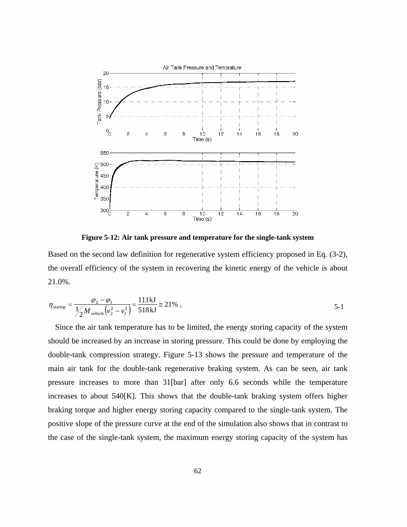
62
Figure 5-12: Air tank pressure and temperature for the single-tank system
Based on the second law definition for regenerative system efficiency proposed in Eq. (3-2),
the overall efficiency of the system in recovering the kinetic energy of the vehicle is about
21.0%.
( ) ,%21kJ518kJ111
21 2
122
12startup ≅=
−
−=
vvM vehicle
ϕϕη 5-1
Since the air tank temperature has to be limited, the energy storing capacity of the system
should be increased by an increase in storing pressure. This could be done by employing the
double-tank compression strategy. Figure 5-13 shows the pressure and temperature of the
main air tank for the double-tank regenerative braking system. As can be seen, air tank
pressure increases to more than 31[bar] after only 6.6 seconds while the temperature
increases to about 540[K]. This shows that the double-tank braking system offers higher
braking torque and higher energy storing capacity compared to the single-tank system. The
positive slope of the pressure curve at the end of the simulation also shows that in contrast to
the case of the single-tank system, the maximum energy storing capacity of the system has
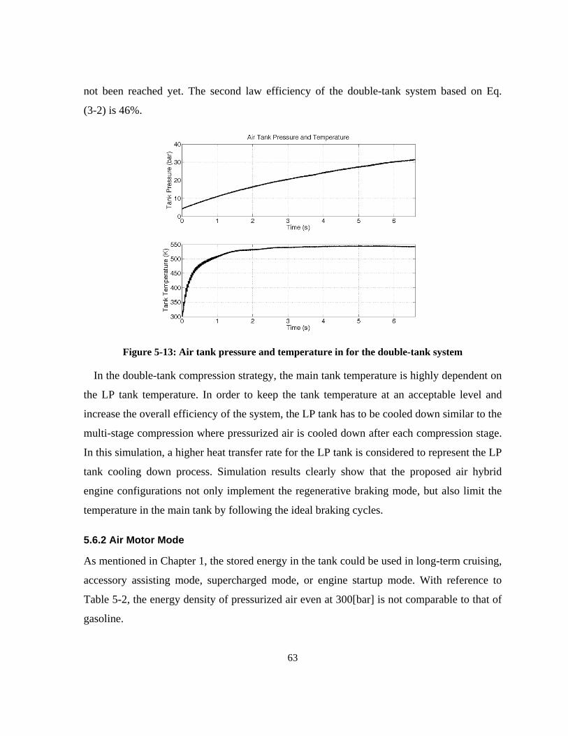
63
not been reached yet. The second law efficiency of the double-tank system based on Eq.
(3-2) is 46%.
Figure 5-13: Air tank pressure and temperature in for the double-tank system
In the double-tank compression strategy, the main tank temperature is highly dependent on
the LP tank temperature. In order to keep the tank temperature at an acceptable level and
increase the overall efficiency of the system, the LP tank has to be cooled down similar to the
multi-stage compression where pressurized air is cooled down after each compression stage.
In this simulation, a higher heat transfer rate for the LP tank is considered to represent the LP
tank cooling down process. Simulation results clearly show that the proposed air hybrid
engine configurations not only implement the regenerative braking mode, but also limit the
temperature in the main tank by following the ideal braking cycles.
5.6.2 Air Motor Mode
As mentioned in Chapter 1, the stored energy in the tank could be used in long-term cruising,
accessory assisting mode, supercharged mode, or engine startup mode. With reference to
Table 5-2, the energy density of pressurized air even at 300[bar] is not comparable to that of
gasoline.
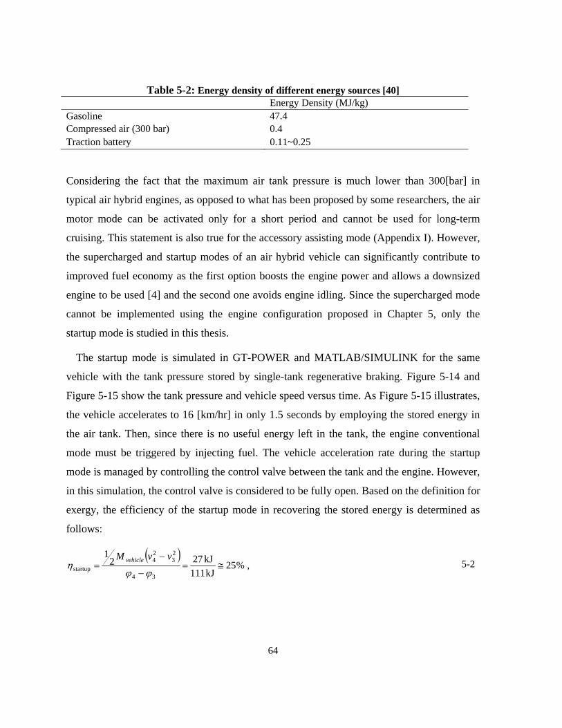
64
Table 5-2: Energy density of different energy sources [40] Energy Density (MJ/kg) Gasoline 47.4 Compressed air (300 bar) 0.4 Traction battery 0.11~0.25
Considering the fact that the maximum air tank pressure is much lower than 300[bar] in
typical air hybrid engines, as opposed to what has been proposed by some researchers, the air
motor mode can be activated only for a short period and cannot be used for long-term
cruising. This statement is also true for the accessory assisting mode (Appendix I). However,
the supercharged and startup modes of an air hybrid vehicle can significantly contribute to
improved fuel economy as the first option boosts the engine power and allows a downsized
engine to be used [4] and the second one avoids engine idling. Since the supercharged mode
cannot be implemented using the engine configuration proposed in Chapter 5, only the
startup mode is studied in this thesis.
The startup mode is simulated in GT-POWER and MATLAB/SIMULINK for the same
vehicle with the tank pressure stored by single-tank regenerative braking. Figure 5-14 and
Figure 5-15 show the tank pressure and vehicle speed versus time. As Figure 5-15 illustrates,
the vehicle accelerates to 16 [km/hr] in only 1.5 seconds by employing the stored energy in
the air tank. Then, since there is no useful energy left in the tank, the engine conventional
mode must be triggered by injecting fuel. The vehicle acceleration rate during the startup
mode is managed by controlling the control valve between the tank and the engine. However,
in this simulation, the control valve is considered to be fully open. Based on the definition for
exergy, the efficiency of the startup mode in recovering the stored energy is determined as
follows:
( ),%25
kJ111kJ272
1
34
23
24
startup ≅=−
−=
ϕϕη
vvM vehicle 5-2
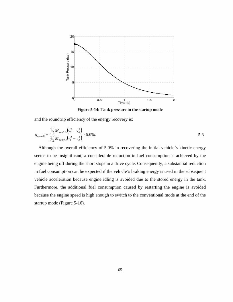
65
Figure 5-14: Tank pressure in the startup mode
and the roundtrip efficiency of the energy recovery is:
( )( ) %.0.5
21
21
22
21
24
23
overall ≅−
−=
vvM
vvM
vehicle
vehicleη 5-3
Although the overall efficiency of 5.0% in recovering the initial vehicle’s kinetic energy
seems to be insignificant, a considerable reduction in fuel consumption is achieved by the
engine being off during the short stops in a drive cycle. Consequently, a substantial reduction
in fuel consumption can be expected if the vehicle’s braking energy is used in the subsequent
vehicle acceleration because engine idling is avoided due to the stored energy in the tank.
Furthermore, the additional fuel consumption caused by restarting the engine is avoided
because the engine speed is high enough to switch to the conventional mode at the end of the
startup mode (Figure 5-16).
0 0.5 1 1.5 20
5
10
15
20
Time (s)
Tan
k P
ress
ure
(bar
)
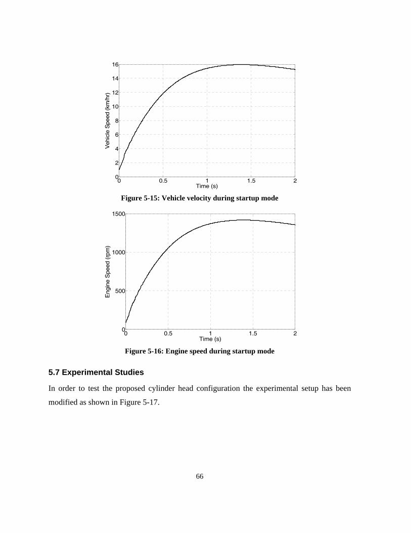
66
Figure 5-15: Vehicle velocity during startup mode
Figure 5-16: Engine speed during startup mode
5.7 Experimental Studies
In order to test the proposed cylinder head configuration the experimental setup has been
modified as shown in Figure 5-17.
0 0.5 1 1.5 20
2
4
6
8
10
12
14
16
Time (s)
Veh
icle
Spe
ed (
km/h
r)
0 0.5 1 1.5 20
500
1000
1500
Time (s)
Eng
ine
Spe
ed (
rpm
)
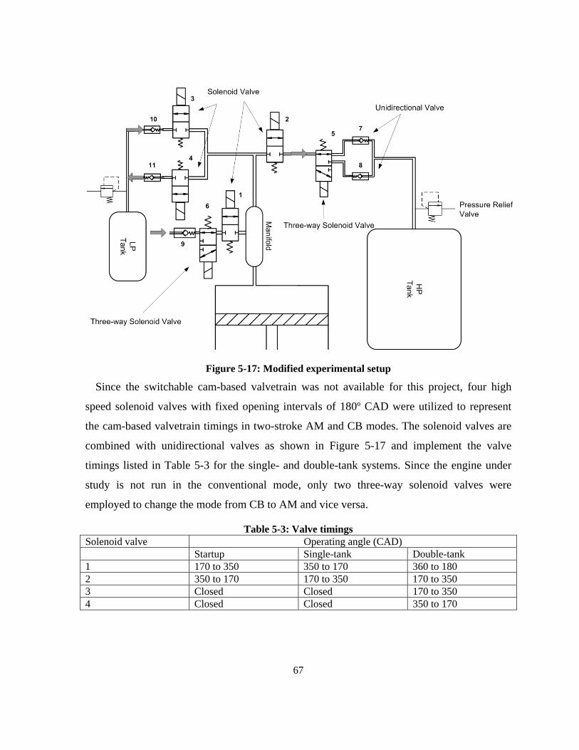
67
Figure 5-17: Modified experimental setup Since the switchable cam-based valvetrain was not available for this project, four high
speed solenoid valves with fixed opening intervals of 180º CAD were utilized to represent
the cam-based valvetrain timings in two-stroke AM and CB modes. The solenoid valves are
combined with unidirectional valves as shown in Figure 5-17 and implement the valve
timings listed in Table 5-3 for the single- and double-tank systems. Since the engine under
study is not run in the conventional mode, only two three-way solenoid valves were
employed to change the mode from CB to AM and vice versa.
Table 5-3: Valve timings Solenoid valve Operating angle (CAD) Startup Single-tank Double-tank 1 170 to 350 350 to 170 360 to 180 2 350 to 170 170 to 350 170 to 350 3 Closed Closed 170 to 350 4 Closed Closed 350 to 170
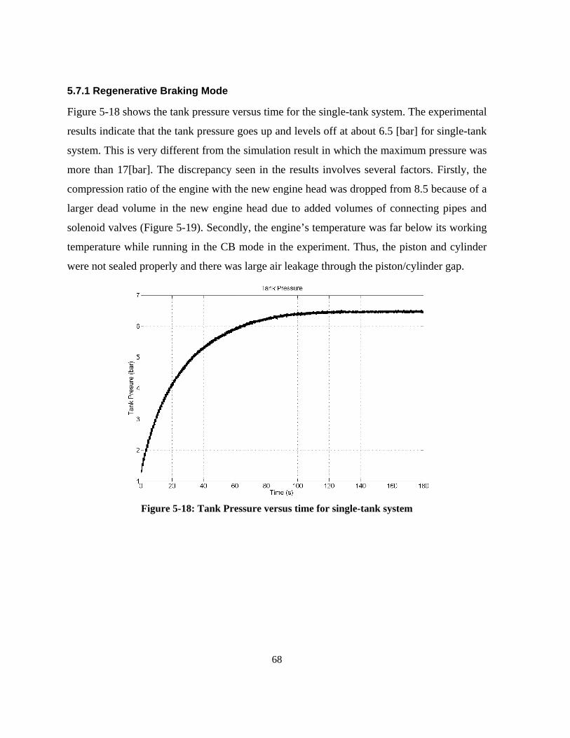
68
5.7.1 Regenerative Braking Mode
Figure 5-18 shows the tank pressure versus time for the single-tank system. The experimental
results indicate that the tank pressure goes up and levels off at about 6.5 [bar] for single-tank
system. This is very different from the simulation result in which the maximum pressure was
more than 17[bar]. The discrepancy seen in the results involves several factors. Firstly, the
compression ratio of the engine with the new engine head was dropped from 8.5 because of a
larger dead volume in the new engine head due to added volumes of connecting pipes and
solenoid valves (Figure 5-19). Secondly, the engine’s temperature was far below its working
temperature while running in the CB mode in the experiment. Thus, the piston and cylinder
were not sealed properly and there was large air leakage through the piston/cylinder gap.
Figure 5-18: Tank Pressure versus time for single-tank system
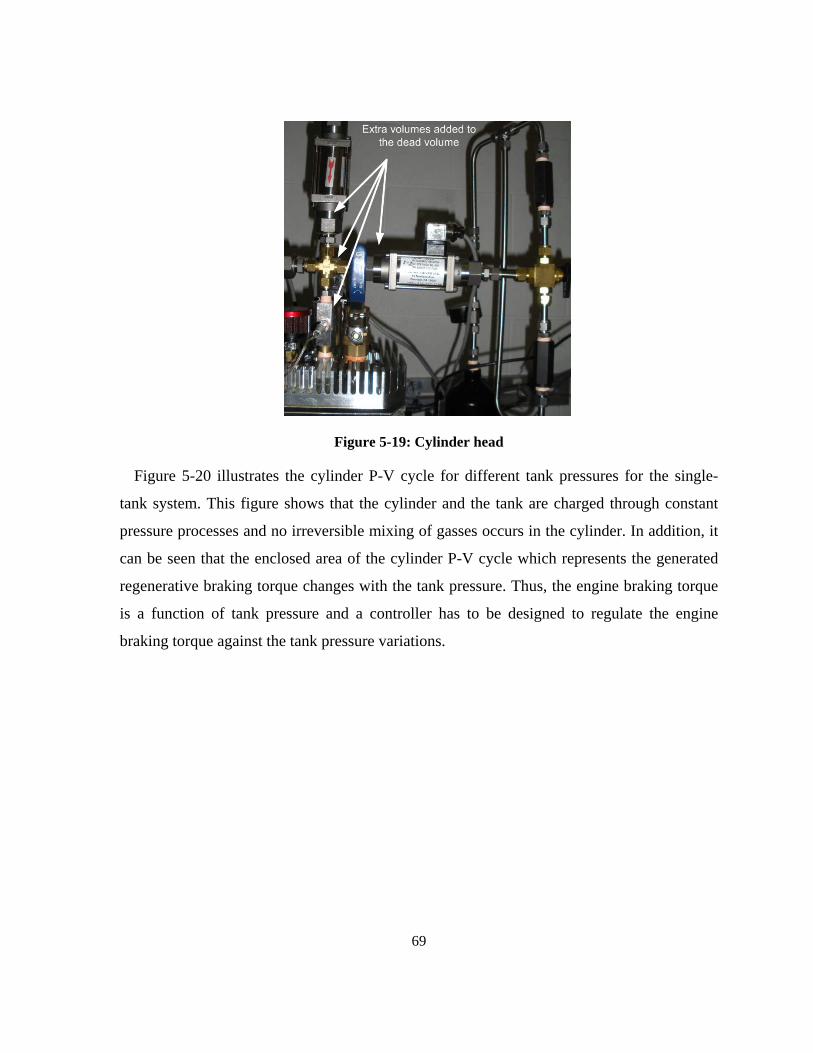
69
Figure 5-19: Cylinder head
Figure 5-20 illustrates the cylinder P-V cycle for different tank pressures for the single-
tank system. This figure shows that the cylinder and the tank are charged through constant
pressure processes and no irreversible mixing of gasses occurs in the cylinder. In addition, it
can be seen that the enclosed area of the cylinder P-V cycle which represents the generated
regenerative braking torque changes with the tank pressure. Thus, the engine braking torque
is a function of tank pressure and a controller has to be designed to regulate the engine
braking torque against the tank pressure variations.
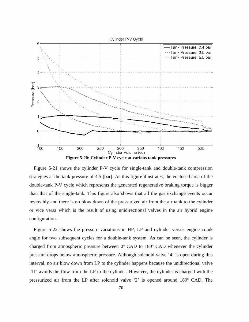
70
Figure 5-20: Cylinder P-V cycle at various tank pressures
Figure 5-21 shows the cylinder P-V cycle for single-tank and double-tank compression
strategies at the tank pressure of 4.5 [bar]. As this figure illustrates, the enclosed area of the
double-tank P-V cycle which represents the generated regenerative braking torque is bigger
than that of the single-tank. This figure also shows that all the gas exchange events occur
reversibly and there is no blow down of the pressurized air from the air tank to the cylinder
or vice versa which is the result of using unidirectional valves in the air hybrid engine
configuration.
Figure 5-22 shows the pressure variations in HP, LP and cylinder versus engine crank
angle for two subsequent cycles for a double-tank system. As can be seen, the cylinder is
charged from atmospheric pressure between 0º CAD to 180º CAD whenever the cylinder
pressure drops below atmospheric pressure. Although solenoid valve ‘4’ is open during this
interval, no air blow down from LP to the cylinder happens because the unidirectional valve
‘11’ avoids the flow from the LP to the cylinder. However, the cylinder is charged with the
pressurized air from the LP after solenoid valve ‘2’ is opened around 180º CAD. The
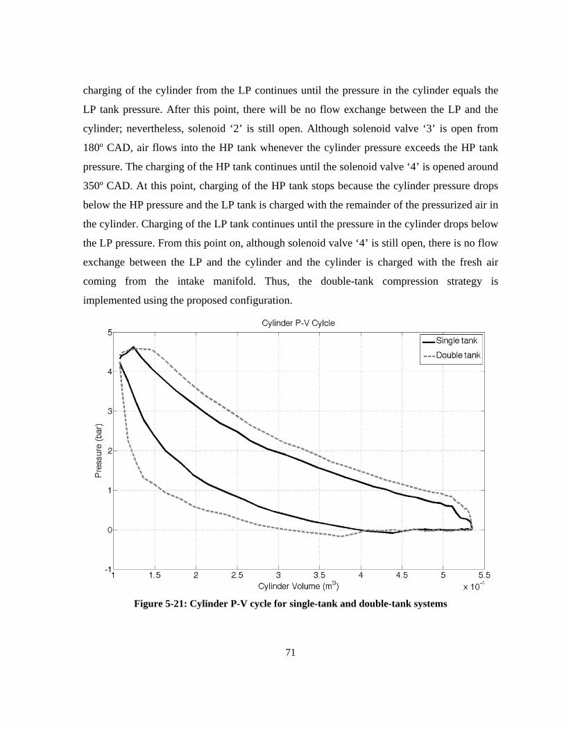
71
charging of the cylinder from the LP continues until the pressure in the cylinder equals the
LP tank pressure. After this point, there will be no flow exchange between the LP and the
cylinder; nevertheless, solenoid ‘2’ is still open. Although solenoid valve ‘3’ is open from
180º CAD, air flows into the HP tank whenever the cylinder pressure exceeds the HP tank
pressure. The charging of the HP tank continues until the solenoid valve ‘4’ is opened around
350º CAD. At this point, charging of the HP tank stops because the cylinder pressure drops
below the HP pressure and the LP tank is charged with the remainder of the pressurized air in
the cylinder. Charging of the LP tank continues until the pressure in the cylinder drops below
the LP pressure. From this point on, although solenoid valve ‘4’ is still open, there is no flow
exchange between the LP and the cylinder and the cylinder is charged with the fresh air
coming from the intake manifold. Thus, the double-tank compression strategy is
implemented using the proposed configuration.
Figure 5-21: Cylinder P-V cycle for single-tank and double-tank systems
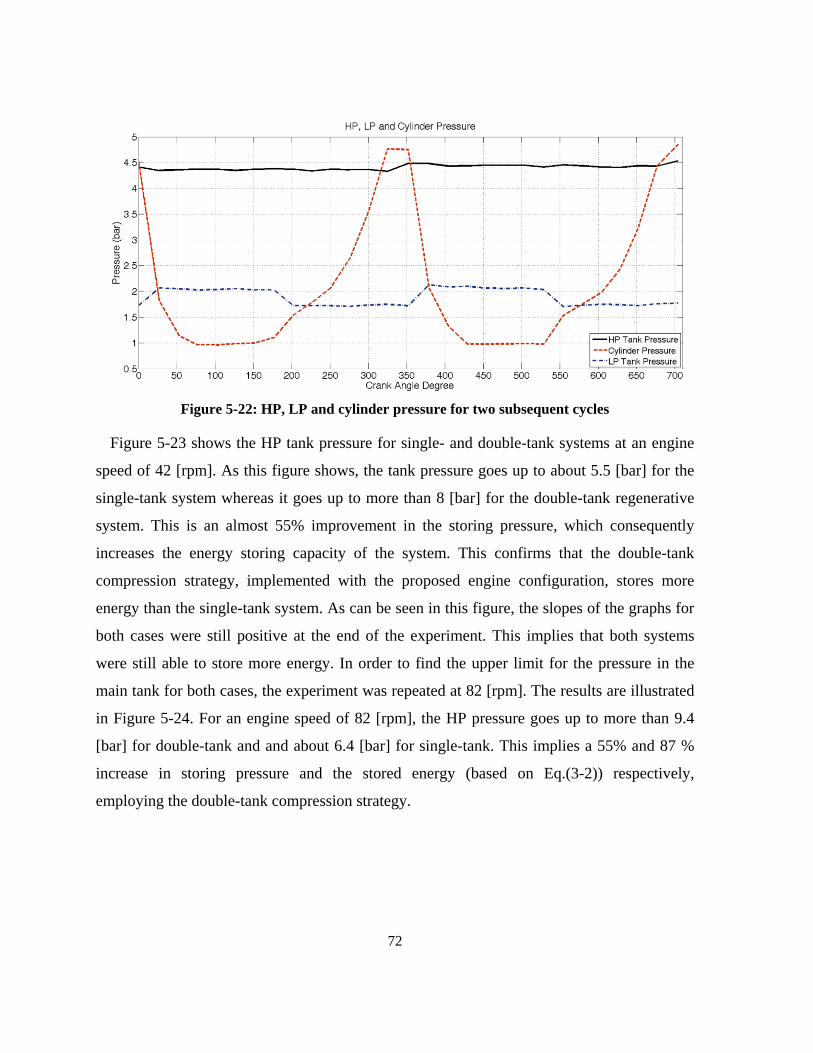
72
Figure 5-22: HP, LP and cylinder pressure for two subsequent cycles
Figure 5-23 shows the HP tank pressure for single- and double-tank systems at an engine
speed of 42 [rpm]. As this figure shows, the tank pressure goes up to about 5.5 [bar] for the
single-tank system whereas it goes up to more than 8 [bar] for the double-tank regenerative
system. This is an almost 55% improvement in the storing pressure, which consequently
increases the energy storing capacity of the system. This confirms that the double-tank
compression strategy, implemented with the proposed engine configuration, stores more
energy than the single-tank system. As can be seen in this figure, the slopes of the graphs for
both cases were still positive at the end of the experiment. This implies that both systems
were still able to store more energy. In order to find the upper limit for the pressure in the
main tank for both cases, the experiment was repeated at 82 [rpm]. The results are illustrated
in Figure 5-24. For an engine speed of 82 [rpm], the HP pressure goes up to more than 9.4
[bar] for double-tank and and about 6.4 [bar] for single-tank. This implies a 55% and 87 %
increase in storing pressure and the stored energy (based on Eq.(3-2)) respectively,
employing the double-tank compression strategy.
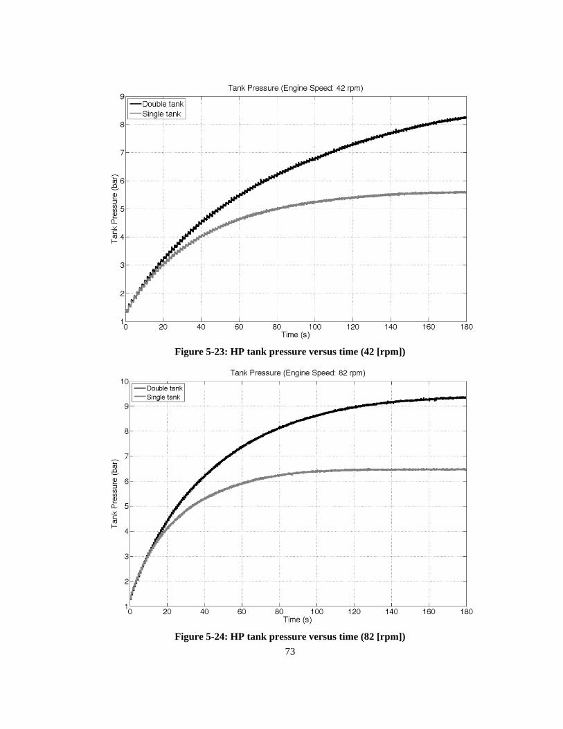
73
Figure 5-23: HP tank pressure versus time (42 [rpm])
Figure 5-24: HP tank pressure versus time (82 [rpm])
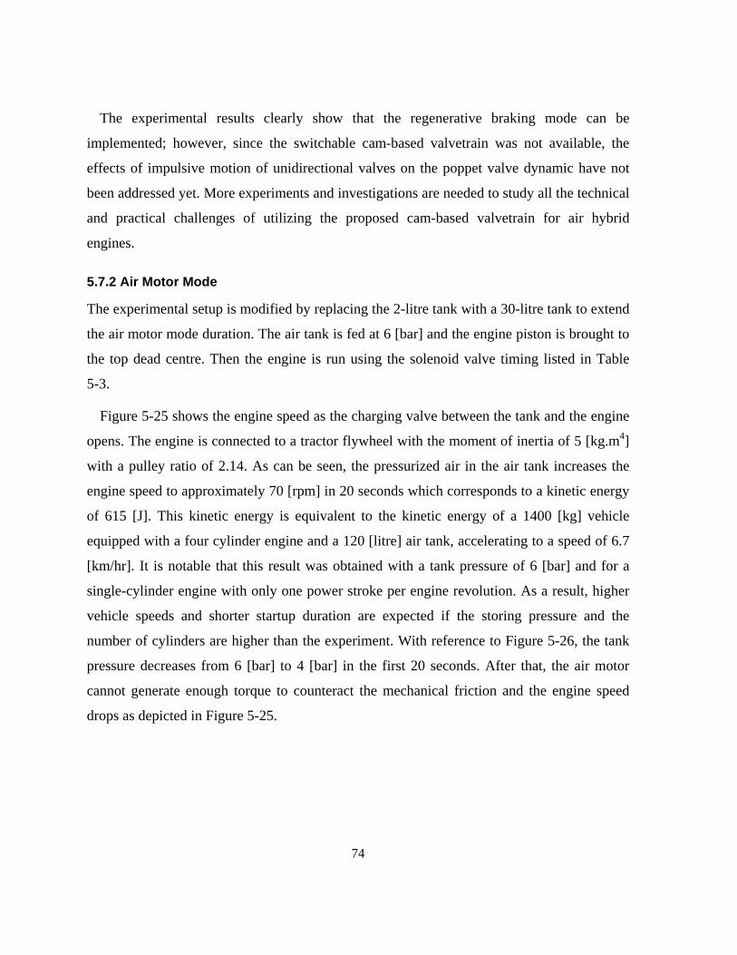
74
The experimental results clearly show that the regenerative braking mode can be
implemented; however, since the switchable cam-based valvetrain was not available, the
effects of impulsive motion of unidirectional valves on the poppet valve dynamic have not
been addressed yet. More experiments and investigations are needed to study all the technical
and practical challenges of utilizing the proposed cam-based valvetrain for air hybrid
engines.
5.7.2 Air Motor Mode
The experimental setup is modified by replacing the 2-litre tank with a 30-litre tank to extend
the air motor mode duration. The air tank is fed at 6 [bar] and the engine piston is brought to
the top dead centre. Then the engine is run using the solenoid valve timing listed in Table
5-3.
Figure 5-25 shows the engine speed as the charging valve between the tank and the engine
opens. The engine is connected to a tractor flywheel with the moment of inertia of 5 [kg.m4]
with a pulley ratio of 2.14. As can be seen, the pressurized air in the air tank increases the
engine speed to approximately 70 [rpm] in 20 seconds which corresponds to a kinetic energy
of 615 [J]. This kinetic energy is equivalent to the kinetic energy of a 1400 [kg] vehicle
equipped with a four cylinder engine and a 120 [litre] air tank, accelerating to a speed of 6.7
[km/hr]. It is notable that this result was obtained with a tank pressure of 6 [bar] and for a
single-cylinder engine with only one power stroke per engine revolution. As a result, higher
vehicle speeds and shorter startup duration are expected if the storing pressure and the
number of cylinders are higher than the experiment. With reference to Figure 5-26, the tank
pressure decreases from 6 [bar] to 4 [bar] in the first 20 seconds. After that, the air motor
cannot generate enough torque to counteract the mechanical friction and the engine speed
drops as depicted in Figure 5-25.
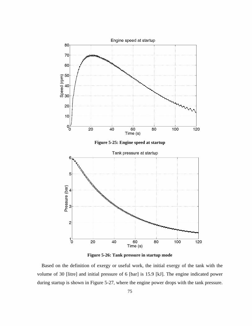
75
Figure 5-25: Engine speed at startup
Figure 5-26: Tank pressure in startup mode
Based on the definition of exergy or useful work, the initial exergy of the tank with the
volume of 30 [litre] and initial pressure of 6 [bar] is 15.9 [kJ]. The engine indicated power
during startup is shown in Figure 5-27, where the engine power drops with the tank pressure.
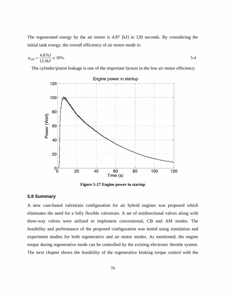
76
The regenerated energy by the air motor is 4.87 [kJ] in 120 seconds. By considering the
initial tank exergy, the overall efficiency of air motor mode is:
%.309.15
87.4AM ≅=
kJkJη 5-4
The cylinder/piston leakage is one of the important factors in the low air motor efficiency.
Figure 5-27 Engine power in startup
5.8 Summary
A new cam-based valvetrain configuration for air hybrid engines was proposed which
eliminates the need for a fully flexible valvetrain. A set of unidirectional valves along with
three-way valves were utilized to implement conventional, CB and AM modes. The
feasibility and performance of the proposed configuration was tested using simulation and
experiment studies for both regenerative and air motor modes. As mentioned, the engine
torque during regenerative mode can be controlled by the existing electronic throttle system.
The next chapter shows the feasibility of the regenerative braking torque control with the

77
throttle and presents the design and implementation of model-based and model-free
controllers for this purpose.
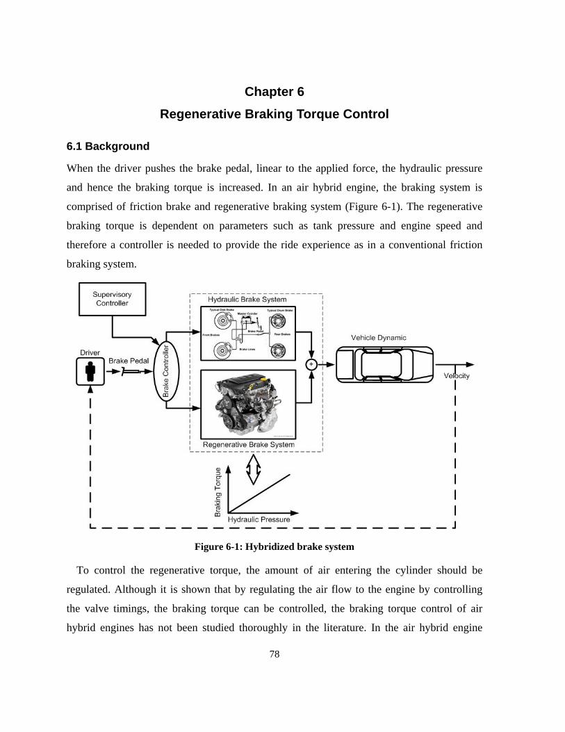
78
Chapter 6 Regenerative Braking Torque Control
6.1 Background
When the driver pushes the brake pedal, linear to the applied force, the hydraulic pressure
and hence the braking torque is increased. In an air hybrid engine, the braking system is
comprised of friction brake and regenerative braking system (Figure 6-1). The regenerative
braking torque is dependent on parameters such as tank pressure and engine speed and
therefore a controller is needed to provide the ride experience as in a conventional friction
braking system.
Figure 6-1: Hybridized brake system
To control the regenerative torque, the amount of air entering the cylinder should be
regulated. Although it is shown that by regulating the air flow to the engine by controlling
the valve timings, the braking torque can be controlled, the braking torque control of air
hybrid engines has not been studied thoroughly in the literature. In the air hybrid engine
79
configuration proposed in Chapter 5, the regenerative braking torque is controlled by
regulating the throttle angle. By controlling the throttle angle, one can control the manifold
pressure and consequently the engine braking torque. The main objective of this chapter is to
develop a throttle-based braking torque control for the proposed air hybrid engine. This
controller should be robust and be able to track the desired braking torque.
Model free controllers such as proportional-integral (PI) controllers along with lookup
tables are usually used in engine controls [41]. Although these control strategies offer
satisfactory performance, the wide range of engine operating conditions, inherent non-
linearity and controller calibrations have motivated researchers to conduct many studies on
model-based controllers [41]. For instance, Souder et al [42] designed an adaptive sliding
mode controller based on the mean value model of the engine to control the air-fuel ratio.
Wagner et al. [41] designed a backstepping controller for simultaneous air to fuel ratio and
engine speed control. Tang et al. [43] designed an adaptive feedback linearization based
controller to control the air fuel ratio in spark ignition engines. The authors showed that,
using nonlinear controllers leads to better closed-loop performance than conventional model-
free or lookup table controllers.
There are several techniques for controlling nonlinear dynamic systems. However, the
robust sliding mode controllers (SMC) have widely been used in many practical applications
due to their capability to deal with uncertainties, good transient performance and their
simplicity [44]. Furthermore, these control techniques could provide a systematic approach to
maintain both stability and performance in the presence of modeling uncertainties [44].
In this chapter, the adaptive sliding mode controller is used for the engine regenerative
braking torque control. This controller plus other model-free controllers are used in
simulation and experiments for evaluation.
6.2 Regenerative Braking Mean Value Model (MVM)
The first step in designing a model-based controller for the engine in compression braking
mode is deriving a control oriented model. This section is devoted to deriving an MVM for
the engine during braking.
80
An MVM is a dynamic model of an engine that requires little engine data [45]. For a
typical SI engine, MVM is comprised of three main subsystems [45], [46]: the fueling
dynamics, the crank shaft dynamics and the manifold air dynamics. However, for an air
hybrid engine in the regenerative mode, only the latter two subsystems are needed for the
mean value model.
Air mass flow rate through the throttle in MVM is a function of manifold pressure and
throttle angle that can be expressed by [47]:
( ) ( ) ,rairthrottle PAm ψθρ=& 6-1
where ( )rPψ is:
( )( )
,
53.011
2
53.01
21
2
11
11
⎪⎪⎪
⎩
⎪⎪⎪
⎨
⎧
≥⎥⎥⎦
⎤
⎢⎢⎣
⎡−
−
<+⎟⎟
⎠
⎞⎜⎜⎝
⎛+
=−
−
rrmanair
r
rmanair
r
PPM
RP
PM
R
Pγγ
γ
γ
γγυ
γυγ
γψ 6-2
and ( )θA is the throttle effective area and is estimated by :
( ) ),(0 θθ dCAA = 6-3
where 0A is the throttle reference area and )(θdC is the discharge coefficient which is
defined experimentally as a function of throttle angle. Mass flow rate to the engine is defined
by speed-density equation as:
( ) ,,,2 tankPPV
RMPm mdatm
airatmengine ωη
πω
υ=& 6-4
where ( )tank,, PPmvol ωη is the engine volumetric efficiency and is a function of manifold
pressure and engine speed for typical engines [47]. However, in the case of air hybrid
engines in the compression braking mode, tank pressure has a direct effect on the value of
volumetric efficiency. As the tank pressure increases, the volumetric efficiency drops
because the leftover pressurized air in the cylinder decreases the air flow rate to the engine.
Thus, engine volumetric efficiency in the regenerative mode is considered to be a function of
81
the manifold pressure, engine speed and tank pressure. The manifold pressure dynamic,
assuming constant manifold temperature is derived using the conservation of air mass in the
intake manifold and the ideal gas law:
( ).enginethrottleairman
manm mm
MVRP &&& −=υ
6-5
Now, we need to derive an expression for the engine torque as a function of air mass flow
rate to the engine. In the MVM for SI engines, the engine torque is related to the air mass
flow rate by considering the engine thermal efficiency map and the heat content of the
injected fuel. However, there is no fuel injection during the CB mode. Therefore, a new
model is needed to relate the air mass flow rate to the engine torque. In the regenerative
braking mode, the engine can be considered in a steady state mode which receives air at the
manifold pressure and compresses it adiabatically to the tank pressure. Thus, the engine
braking torque can be estimated by:
.
1
1
tank
ωυ
γγ
⎟⎟⎟
⎠
⎞
⎜⎜⎜
⎝
⎛−⎟⎟
⎠
⎞⎜⎜⎝
⎛
=
−
atm
pmanengineengine
PP
CmT &
6-6
In the above equation, the engine friction and heat transfer from the cylinder are ignored. To
incorporate both of these parameters, the above equation is modified to:
( ) ,,,
1
tank
1
tank
PPTPPCm
T mf
atmpmanengine
engine ωω
υγγ
+⎟⎟⎟
⎠
⎞
⎜⎜⎜
⎝
⎛−⎟⎟
⎠
⎞⎜⎜⎝
⎛
=
−
&
6-7
where, ( )tank,, PPT mf ω accounts for the engine friction and heat transfer that can be found
through experiment. Replacing enginem& from Eq. (6-4) results in:
( ) ,,,121
tank
1
tank PPTPPCV
RMPT mf
atmpmanvold
atm
atmengine ωυη
πυ
γγ
+⎟⎟⎟
⎠
⎞
⎜⎜⎜
⎝
⎛−⎟⎟
⎠
⎞⎜⎜⎝
⎛⎟⎟⎠
⎞⎜⎜⎝
⎛=
−
6-8
82
Differentiating the above equation with respect to time and assuming that t∂∂ω and
tP ∂∂ tank are negligible compared to the manifold pressure dynamic (the air tank is at least
two order of magnitude larger than the manifold) leads to:
.121
1
tankm
m
fm
atmpman
m
vold
atm
atmengine P
PT
PPPC
PV
RMPT &&&
∂∂
+⎟⎟⎟
⎠
⎞
⎜⎜⎜
⎝
⎛−⎟⎟
⎠
⎞⎜⎜⎝
⎛⎟⎟⎠
⎞⎜⎜⎝
⎛∂∂
=
+−γγ
υηπυ
6-9
For convenience, the above equation can be written as:
,1 mengine PfT && = 6-10
where, .121
1
tank1
m
fatmpman
m
vold
atm
atm
PT
PPC
PV
RMPf
∂∂
+⎟⎟⎟
⎠
⎞
⎜⎜⎜
⎝
⎛−⎟⎟
⎠
⎞⎜⎜⎝
⎛⎟⎟⎠
⎞⎜⎜⎝
⎛∂∂
=
+−γγ
νηπυ
Substituting mP& from Eq.
(6-5) in Eq. (6-10) yields:
.2
)()(1 ⎟⎟⎠
⎞⎜⎜⎝
⎛−= vold
atm
mrair
man
manengine V
RMPPA
MVRfT η
πω
υψθρυ& 6-11
Now, the above equation can be written as the following control affine system (for more
information on control affine systems see [44]):
,)( 21 gAgTengine += θ& 6-12
where, ( )( )rman
man PMV
Rfg ψρυ011 = and ⎟⎟
⎠
⎞⎜⎜⎝
⎛−= vold
atm
m
man
man VR
MPMV
Rfg ηπω
υυ
212 .
Now, the engine braking torque is related to the control input, θ , by a non-linear first order
differential equation in a canonical controllable form, Eq. (6-12). In order to check the
validity of the MVM model, a control signal as shown in Figure 6-2.a is applied to both a
detailed engine model in GT-Power with the specifications shown in Table 6-1 and its mean
value model in Matlab/SIMULINK. The mean value model parameters such as volumetric
efficiency maps are obtained from GT-Power detailed model.
83
Table 6-1: Engine specification Number of cylinders 4 Displacement 1800 [cc] Compression ratio 8.5 Throttle diameter 50 [mm]
Figure 6-2.b and Figure 6-2.c show air mass flow rate to the engine and the manifold
pressure obtained from the two models with respect to time. As can be seen, there is a good
agreement between the detailed model and MVM. However, a non-negligible difference
between engine braking torque obtained from GT-Power and MVM can be seen in Figure
6-2.d. The discrepancies seen between the detailed model and MVM can be explained as
follows:
1. MVM is an average model. Thus, the fluctuations caused by the reciprocal operation of the
cylinders cannot be seen in the MVM.
2. Engine volumetric efficiency map ( ( )tank,, PPmvol ωη ), shown in Figure 6-3 for engine speed
of 3000 rpm, is obtained at discrete engine speeds of 500, 1000, 2000, 3000 and 4000 rpm.
The value of volumetric efficiency at the engine speeds different from these values is
obtained by interpolation. This introduces a source of error to the mean value model.
3. The term ( )tank,, PPT mf ω in Eq. (6-7) is neglected in the mean value model. This is the main
source of the discrepancy seen between the detailed model and MVM in Figure 6-2.d. This
difference can be minimized by obtaining a ( )tank,, PPT mf ω map and considering it in the
MVM. However, in this thesis, it is assumed that ( ) 0,, tank =PPT mf ω .
It is a well-known fact that the dynamic model of a system is an approximation of the real
system, due to the presence of complex phenomena and disturbances. Therefore, even though
the derived mean value is not an exact model of the system, it can be used in the design of a
robust model-based controller. Furthermore, the differences between the detailed model and
MVM can be minimized by acquiring the engine operating maps such as ( )tank,, PPm ωη at a
higher number of operating points and including ( )tank,, PPT mf ω in the MVM, but in this
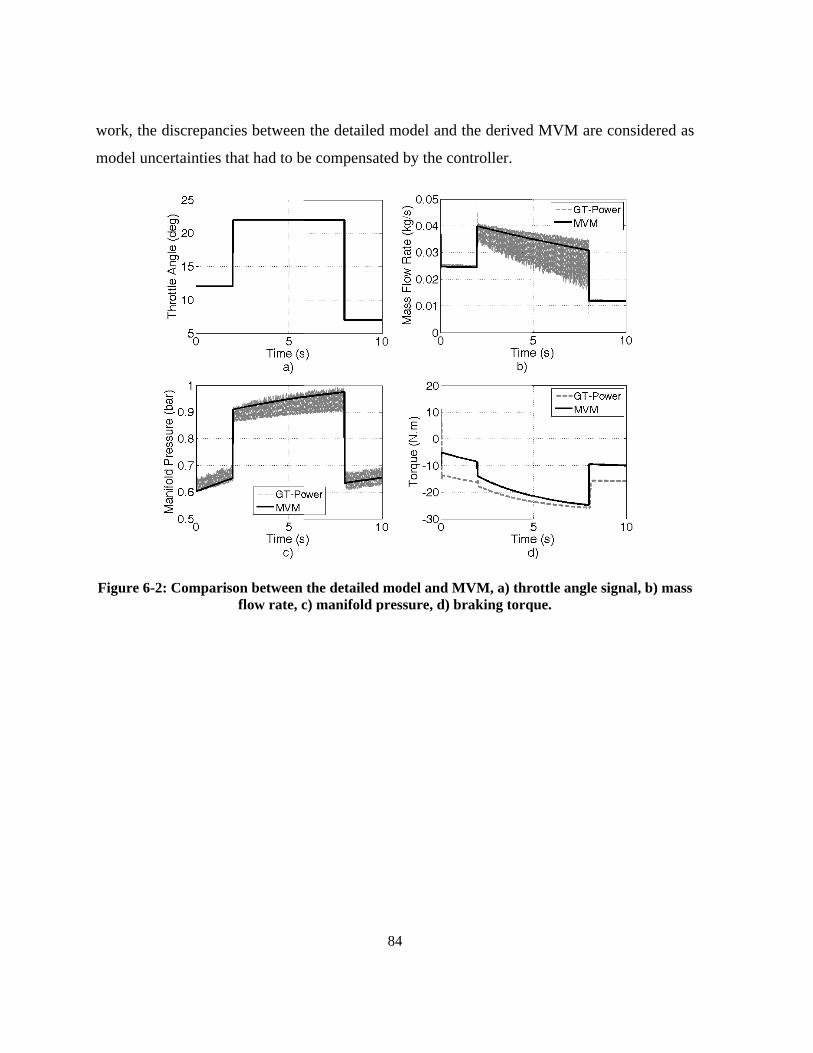
work, the
model un
Figure 6-
e discrepanc
ncertainties t
-2: Comparis
cies between
that had to b
son between flow rate, c
n the detailed
e compensat
the detailed c) manifold p
84
d model and
ted by the co
model and Mpressure, d) b
d the derived
ontroller.
MVM, a) thrbraking torq
d MVM are c
rottle angle sique.
considered a
ignal, b) mas
as
ss
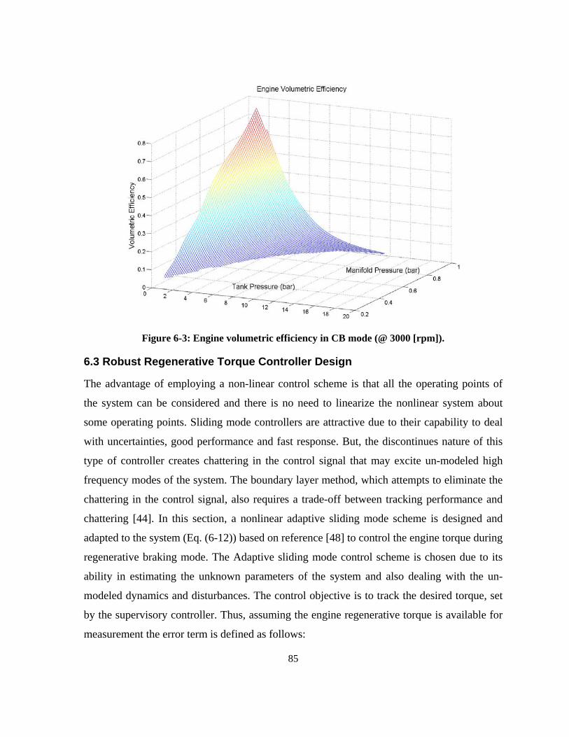
85
Figure 6-3: Engine volumetric efficiency in CB mode (@ 3000 [rpm]).
6.3 Robust Regenerative Torque Controller Design
The advantage of employing a non-linear control scheme is that all the operating points of
the system can be considered and there is no need to linearize the nonlinear system about
some operating points. Sliding mode controllers are attractive due to their capability to deal
with uncertainties, good performance and fast response. But, the discontinues nature of this
type of controller creates chattering in the control signal that may excite un-modeled high
frequency modes of the system. The boundary layer method, which attempts to eliminate the
chattering in the control signal, also requires a trade-off between tracking performance and
chattering [44]. In this section, a nonlinear adaptive sliding mode scheme is designed and
adapted to the system (Eq. (6-12)) based on reference [48] to control the engine torque during
regenerative braking mode. The Adaptive sliding mode control scheme is chosen due to its
ability in estimating the unknown parameters of the system and also dealing with the un-
modeled dynamics and disturbances. The control objective is to track the desired torque, set
by the supervisory controller. Thus, assuming the engine regenerative torque is available for
measurement the error term is defined as follows:
86
.dengine TTe −= 6-13
The first step in designing the SMC is to define/design the sliding surface. In this study, the
integral type sliding surface [44] is chosen to ensure a zero steady-state error.
,0∫ =⎟⎠⎞
⎜⎝⎛ += edt
dtdS
n
λ 6-14
where n is the order of the system. Based on Eq. (6-12), the order of the system is one, thus,
the sliding surface is defined as follows:
.0=+= ∫edteS λ 6-15
The control law that guarantees achieving the above goal is designed systematically in two
steps, which is described next.
6.3.1 Controller Design for Nominal System
In the first step, the design of the SMC for the case of the nominal system (i.e., Eq. (6-12)) is
considered. Then, the control law is designed for the actual system where there are model
uncertainties and external disturbances. Let’s suppose that the system dynamics and all the
model parameters are known at each instant and there are no unknown external disturbances.
One method to design a control law that derives the system trajectories to the sliding surface
is the Lyapunov direct method. Therefore, the following Lyapunov function is considered for
the single-input single-output system defined by Eq. (6-12) as:
.21 SS=Υ 6-16
To guarantee the stability of the system, the derivative of Lyapunv function should satisfy the
following relation:
.0≤=Υ SS && 6-17
If we set Υ& equal to a negative value such as SKSSS −==Υ && where K is a positive constant,
inequality (6-16) is satisfied. Thus,
87
( ) .0=+⇒−= KSSSSKSSS && 6-18
From Eq. (6-15) the derivative of S with respect to time is:
.eTTeeS dengine λλ +−=+= &&&& 6-19
Replacing engineT& from Eq. (6-12) and plugging S& in 0=+ KSS& , results in:
( ) .021 =++−+ KSeTgAg d λθ & 6-20
Thus, the control law for the nominal system is derived as follows:
( )( ) .21
11 KSeTggA d −−+−= −− λθ & 6-21
The standard SMC control law for this system is:
( )( )( ) .sgn21
11 SKeTggA d −−+−= −− λθ & 6-22
Comparing Eq. (6-21), to the standard SMC control law, Eq. (6-22), shows that the
discontinuous signum function, ( )Ssgn , which causes chattering in standard SMC, is replaced
with the continuous function, KS . This removes the chattering from the control input.
However, the smooth control law of (6-21) still needs to be modified as it is not robust to the
model uncertainties and disturbances. There are some other techniques to remove chattering
from the control signal. One of them is the boundary layer method. In the case of boundary
layer method, the control law of (6-22) is replaced with following control law:
( )( )( ) ,/21
11 ελθ SKsateTggA d −−+−= −− & 6-23
where ε is the layer thickness. It can be shown that using the boundary layer method is a
tradeoff between the performance and control discontinuity (Appendix F). Although for a
given system, an optimum value for the thickness can be obtained, the closed-loop system
may not be robust to the plant uncertainties and external disturbances [49].
88
6.3.2 Controller Design for System with Uncertainty
The control law obtained above is valid for a completely known system without any model
uncertainties or external disturbances. However, in the presence of unknown external
disturbances, model and parameters uncertainties, functions 1g and 2g are of the form:
111 ˆ ggg Δ+= , 222 ˆ ggg Δ+= , 6-24
where 1g and 2g are the known parts and 1gΔ and 2gΔ are the unknown parts of 1g and 2g .
Therefore, if the model uncertainties and external disturbances are considered, Eq. (6-12) is
written as:
( ) ( ) ( ).ˆˆ 2211 tdggAgAgTengine +Δ++Δ+= θθ& 6-25
Now, all the uncertain terms can be lumped as follows [48]:
( ) ( ),~21 tdgAgg +Δ+Δ= θ 6-26
and Eq.( 6-12) is rewritten as:
( ) .~ˆˆ 21 ggAgTengine ++= θ& 6-27
For the above system, the control law in Eq. (6-21) has to be modified to:
( )( ) ,~ˆ 21
11 gKSeTggA d −−−+−= −− λθ &)
6-28
however, g~ is unknown and not available in general. Thus, g~ should be replaced by its
estimate, estg~ . Consequently, the control law can be written as:
( )( ) ,~ˆ 21
11
estd gKSeTggA −−−+−= −− λθ &) 6-29
where estg~ is the online estimate of g~ , and is derived in the next section.
6.3.3 Stability and Robustness Analysis
In order to prove the stability of the controller law of (6-29) and to derive an estimation law
for unknown g~ , the following Lyapunov function is considered:
89
( ) ,21 22 Γ+=Υ ES 6-30
where Γ is a positive constant and ggE est~~ −= is the estimation of error. Derivative of the
above function is:
.Γ+=Υ EESS &&& 6-31
From Eq.(6-19), eTTS dengine λ+−= &&& , ( ) ggAgTengine~ˆˆ 21 ++= θ& and
( ) ( )estd gKSeTggA ~ˆ 21
1 −−−+−= − λθ &) . Thus,
( ) ( ),~~11 ggESESKSEEEKSSV est&&&& −Γ+−−=Γ+−−= −− 6-32
now, if the following update law is chosen:
,~ Sgest Γ=& 6-33
the adaptive control law for the system with uncertainties and external disturbances is
defined as:
( )( ).~
~ˆ 21
11
⎪⎩
⎪⎨⎧
Γ=
−−−+−=
∫
−−
Sdtg
gKSeTggA
est
estd λθ &)
6-34
The proposed control law of (6-34) and the dynamic system given in Eq. (6-27) lead to the
following closed-loop dynamics:
,~~ ggKSS est +−=+& 6-35
where estg~ can be replaced by Eq. (6-33) as follows:
.~gSdtKSS =Γ++ ∫& 6-36
Assuming K to be constant, the derivative of the above equation is:
.~gSSKS &&&& =Γ++ 6-37
90
The stability of the above second order system, which is a constant-coefficient Lineard
equation, is studied in[50]. The global asymptotic stability of ( ) ( ) 0=++ xgxxfx &&& can be
proved if all the conditions listed below are satisfied:
I) ( ) 0>xxg ,
II) ( ) 0>xf ,
III) ( ) .lim0
∞=∫∞→ ξξ dgx
x
6-38
Now for the asymptotic stability of the closed-loop system under study (6-35), all of the
above conditions have to be satisfied. The first condition leads to the following inequality:
( ).~~0
~~0~
~0~0~
1
12
222
⎪⎩
⎪⎨⎧
>Γ⇒<Γ⇒<
>Γ⇒>Γ⇒>⇒>Γ⇒
>Γ⇒>−Γ⇒>−Γ
−
−
SggSS
SggSSgSS
gSSgSSSgS
&&
&&&
&&&
6-39
Thus, if Sg&~>Γ is valid, the first condition for global asymptotic stability of the system
is satisfied. If the rate of change of lumped uncertainties is bounded, ∞<< δg&~ , then Sg&~
>Γ
can be satisfied for the whole state space except a small neighborhood of the sliding surface
where ε<S , if εδ
=Γ . Thus, we can conclude that there exists a Γ for which the first
condition of asymptotic stability of the closed loop system is satisfied everywhere in the state
space, except a small neighborhood of the sliding surface if the rate of change of lumped
uncertainties is bounded. The second and third conditions are satisfied because: II) 0>K
and III) ∞=⎟⎟⎠
⎞⎜⎜⎝
⎛−Γ∫∞→
S
S dg
0
lim ξξ
ξ&
. Thus, it can be concluded that the closed-loop system
(6-35) can be brought to any small neighborhood of the sliding surface by choosing a proper
set of control parameters.
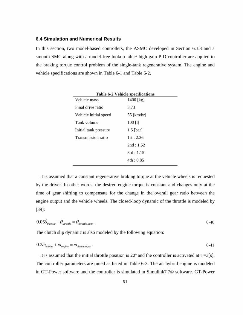
91
6.4 Simulation and Numerical Results
In this section, two model-based controllers, the ASMC developed in Section 6.3.3 and a
smooth SMC along with a model-free lookup table/ high gain PID controller are applied to
the braking torque control problem of the single-tank regenerative system. The engine and
vehicle specifications are shown in Table 6-1 and Table 6-2.
Table 6-2 Vehicle specifications Vehicle mass 1400 [kg]
Final drive ratio 3.73
Vehicle initial speed 55 [km/hr]
Tank volume 100 [l]
Initial tank pressure 1.5 [bar]
Transmission ratio 1st : 2.36
2nd : 1.52
3rd : 1.15
4th : 0.85
It is assumed that a constant regenerative braking torque at the vehicle wheels is requested
by the driver. In other words, the desired engine torque is constant and changes only at the
time of gear shifting to compensate for the change in the overall gear ratio between the
engine output and the vehicle wheels. The closed-loop dynamic of the throttle is modeled by
[39]:
.05.0 ,comthrottlethrottlethrottle θθθ =+& 6-40
The clutch slip dynamic is also modeled by the following equation:
.2.0 outputclutchengineengine ωωω =+& 6-41
It is assumed that the initial throttle position is 20º and the controller is activated at T=3[s].
The controller parameters are tuned as listed in Table 6-3. The air hybrid engine is modeled
in GT-Power software and the controller is simulated in Simulink7.7© software. GT-Power
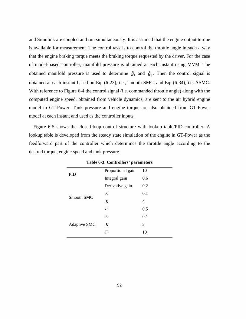
92
and Simulink are coupled and run simultaneously. It is assumed that the engine output torque
is available for measurement. The control task is to control the throttle angle in such a way
that the engine braking torque meets the braking torque requested by the driver. For the case
of model-based controller, manifold pressure is obtained at each instant using MVM. The
obtained manifold pressure is used to determine 1g and 2g . Then the control signal is
obtained at each instant based on Eq. (6-23), i.e., smooth SMC, and Eq. (6-34), i.e, ASMC.
With reference to Figure 6-4 the control signal (i.e. commanded throttle angle) along with the
computed engine speed, obtained from vehicle dynamics, are sent to the air hybrid engine
model in GT-Power. Tank pressure and engine torque are also obtained from GT-Power
model at each instant and used as the controller inputs.
Figure 6-5 shows the closed-loop control structure with lookup table/PID controller. A
lookup table is developed from the steady state simulation of the engine in GT-Power as the
feedforward part of the controller which determines the throttle angle according to the
desired torque, engine speed and tank pressure.
Table 6-3: Controllers’ parameters
PID Proportional gain 10
Integral gain 0.6
Derivative gain 0.2
Smooth SMC λ 0.1
K 4
ε 0.5
Adaptive SMC
λ 0.1
K 2
Γ 10
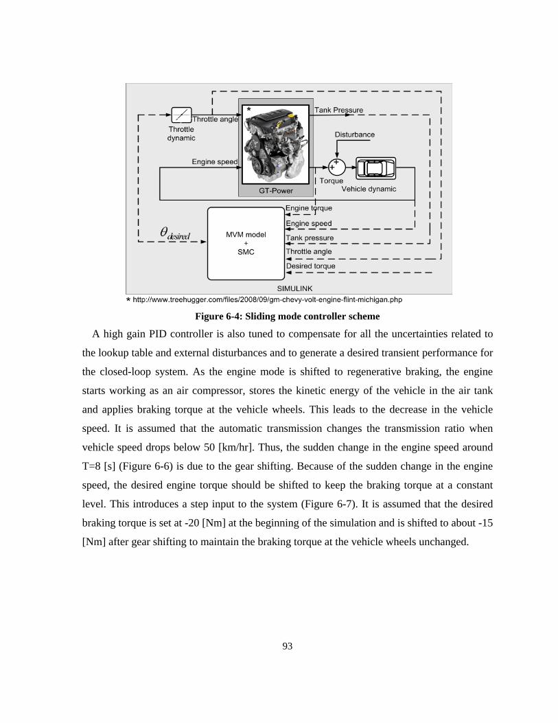
93
Figure 6-4: Sliding mode controller scheme
A high gain PID controller is also tuned to compensate for all the uncertainties related to
the lookup table and external disturbances and to generate a desired transient performance for
the closed-loop system. As the engine mode is shifted to regenerative braking, the engine
starts working as an air compressor, stores the kinetic energy of the vehicle in the air tank
and applies braking torque at the vehicle wheels. This leads to the decrease in the vehicle
speed. It is assumed that the automatic transmission changes the transmission ratio when
vehicle speed drops below 50 [km/hr]. Thus, the sudden change in the engine speed around
T=8 [s] (Figure 6-6) is due to the gear shifting. Because of the sudden change in the engine
speed, the desired engine torque should be shifted to keep the braking torque at a constant
level. This introduces a step input to the system (Figure 6-7). It is assumed that the desired
braking torque is set at -20 [Nm] at the beginning of the simulation and is shifted to about -15
[Nm] after gear shifting to maintain the braking torque at the vehicle wheels unchanged.
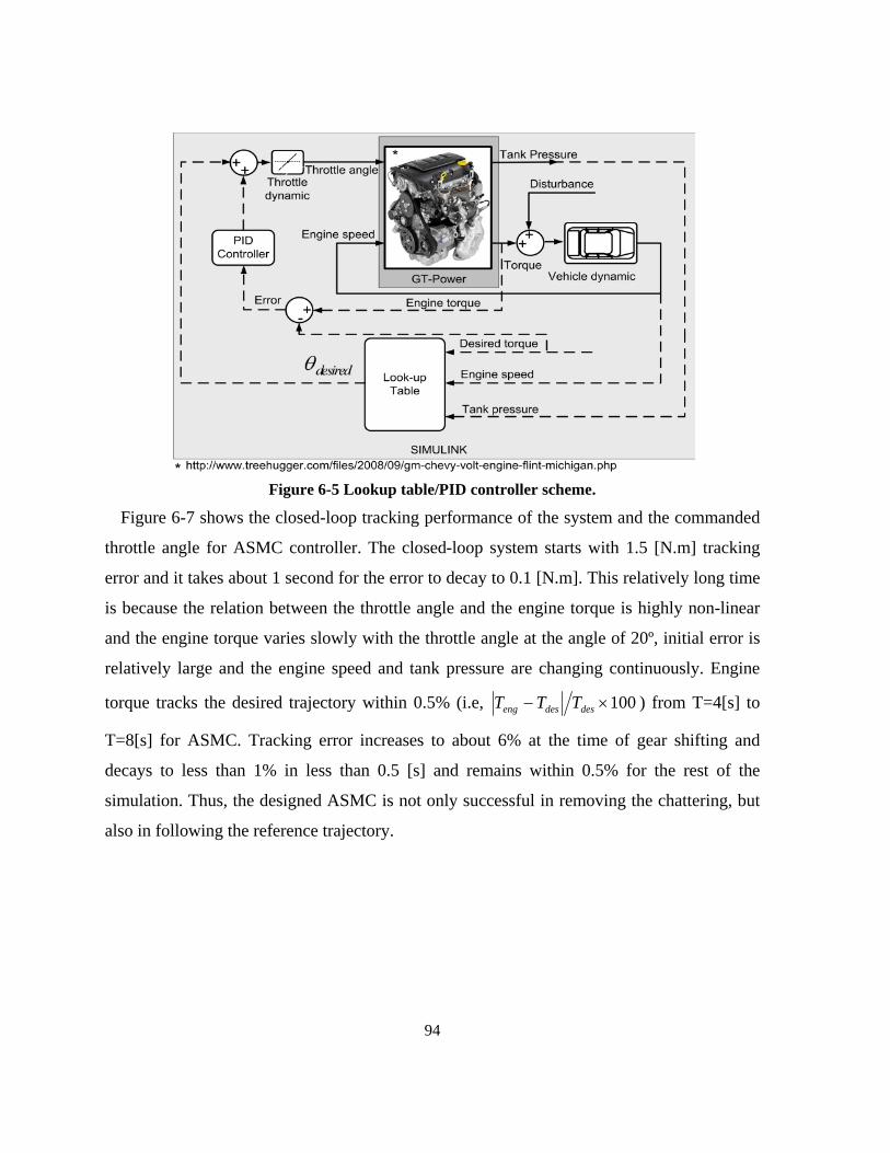
94
Figure 6-5 Lookup table/PID controller scheme.
Figure 6-7 shows the closed-loop tracking performance of the system and the commanded
throttle angle for ASMC controller. The closed-loop system starts with 1.5 [N.m] tracking
error and it takes about 1 second for the error to decay to 0.1 [N.m]. This relatively long time
is because the relation between the throttle angle and the engine torque is highly non-linear
and the engine torque varies slowly with the throttle angle at the angle of 20º, initial error is
relatively large and the engine speed and tank pressure are changing continuously. Engine
torque tracks the desired trajectory within 0.5% (i.e, 100×− desdeseng TTT ) from T=4[s] to
T=8[s] for ASMC. Tracking error increases to about 6% at the time of gear shifting and
decays to less than 1% in less than 0.5 [s] and remains within 0.5% for the rest of the
simulation. Thus, the designed ASMC is not only successful in removing the chattering, but
also in following the reference trajectory.
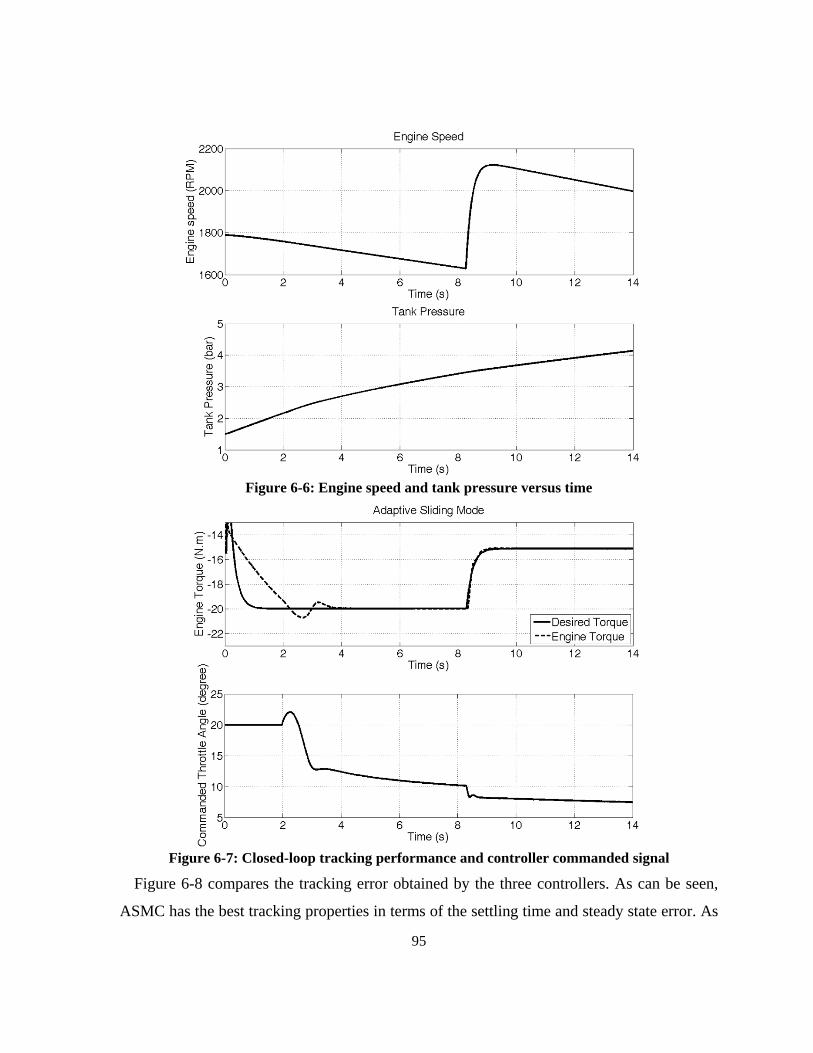
95
Figure 6-6: Engine speed and tank pressure versus time
Figure 6-7: Closed-loop tracking performance and controller commanded signal
Figure 6-8 compares the tracking error obtained by the three controllers. As can be seen,
ASMC has the best tracking properties in terms of the settling time and steady state error. As
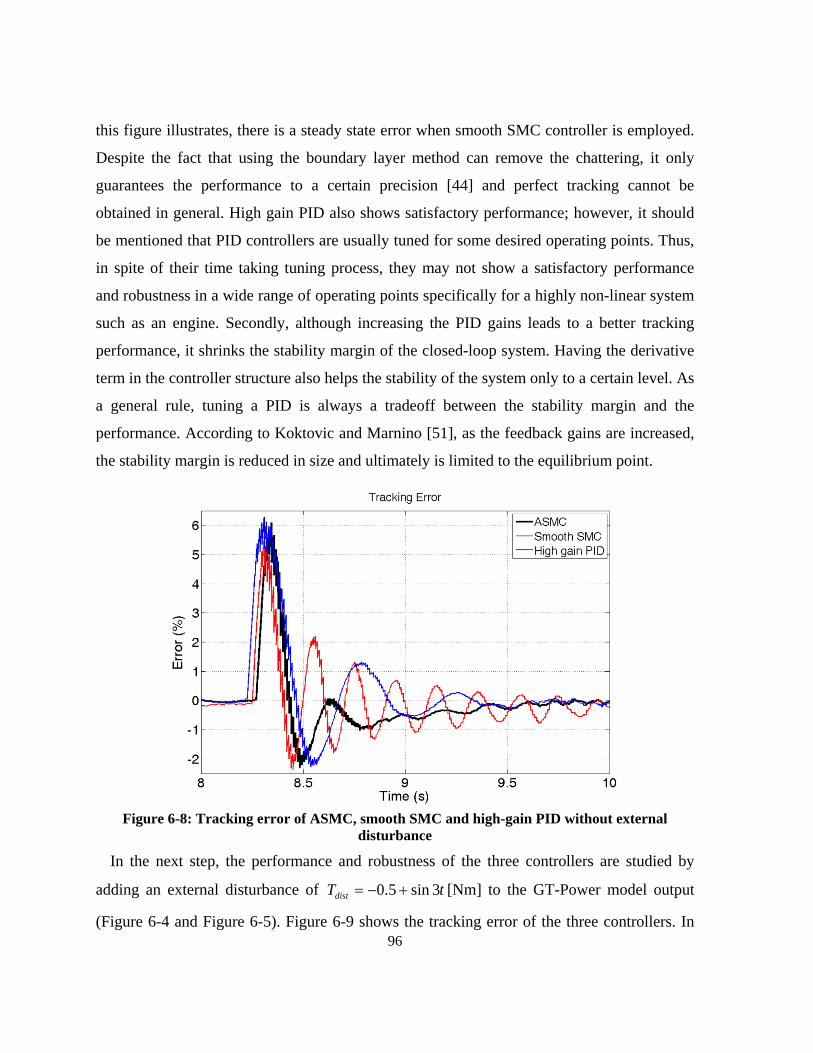
96
this figure illustrates, there is a steady state error when smooth SMC controller is employed.
Despite the fact that using the boundary layer method can remove the chattering, it only
guarantees the performance to a certain precision [44] and perfect tracking cannot be
obtained in general. High gain PID also shows satisfactory performance; however, it should
be mentioned that PID controllers are usually tuned for some desired operating points. Thus,
in spite of their time taking tuning process, they may not show a satisfactory performance
and robustness in a wide range of operating points specifically for a highly non-linear system
such as an engine. Secondly, although increasing the PID gains leads to a better tracking
performance, it shrinks the stability margin of the closed-loop system. Having the derivative
term in the controller structure also helps the stability of the system only to a certain level. As
a general rule, tuning a PID is always a tradeoff between the stability margin and the
performance. According to Koktovic and Marnino [51], as the feedback gains are increased,
the stability margin is reduced in size and ultimately is limited to the equilibrium point.
Figure 6-8: Tracking error of ASMC, smooth SMC and high-gain PID without external
disturbance
In the next step, the performance and robustness of the three controllers are studied by
adding an external disturbance of tTdist 3sin5.0 +−= [Nm] to the GT-Power model output
(Figure 6-4 and Figure 6-5). Figure 6-9 shows the tracking error of the three controllers. In
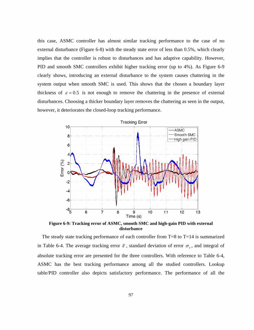
97
this case, ASMC controller has almost similar tracking performance to the case of no
external disturbance (Figure 6-8) with the steady state error of less than 0.5%, which clearly
implies that the controller is robust to disturbances and has adaptive capability. However,
PID and smooth SMC controllers exhibit higher tracking error (up to 4%). As Figure 6-9
clearly shows, introducing an external disturbance to the system causes chattering in the
system output when smooth SMC is used. This shows that the chosen a boundary layer
thickness of 5.0=ε is not enough to remove the chattering in the presence of external
disturbances. Choosing a thicker boundary layer removes the chattering as seen in the output,
however, it deteriorates the closed-loop tracking performance.
Figure 6-9: Tracking error of ASMC, smooth SMC and high-gain PID with external
disturbance
The steady state tracking performance of each controller from T=8 to T=14 is summarized
in Table 6-4. The average tracking error e , standard deviation of error eσ , and integral of
absolute tracking error are presented for the three controllers. With reference to Table 6-4,
ASMC has the best tracking performance among all the studied controllers. Lookup
table/PID controller also depicts satisfactory performance. The performance of all the
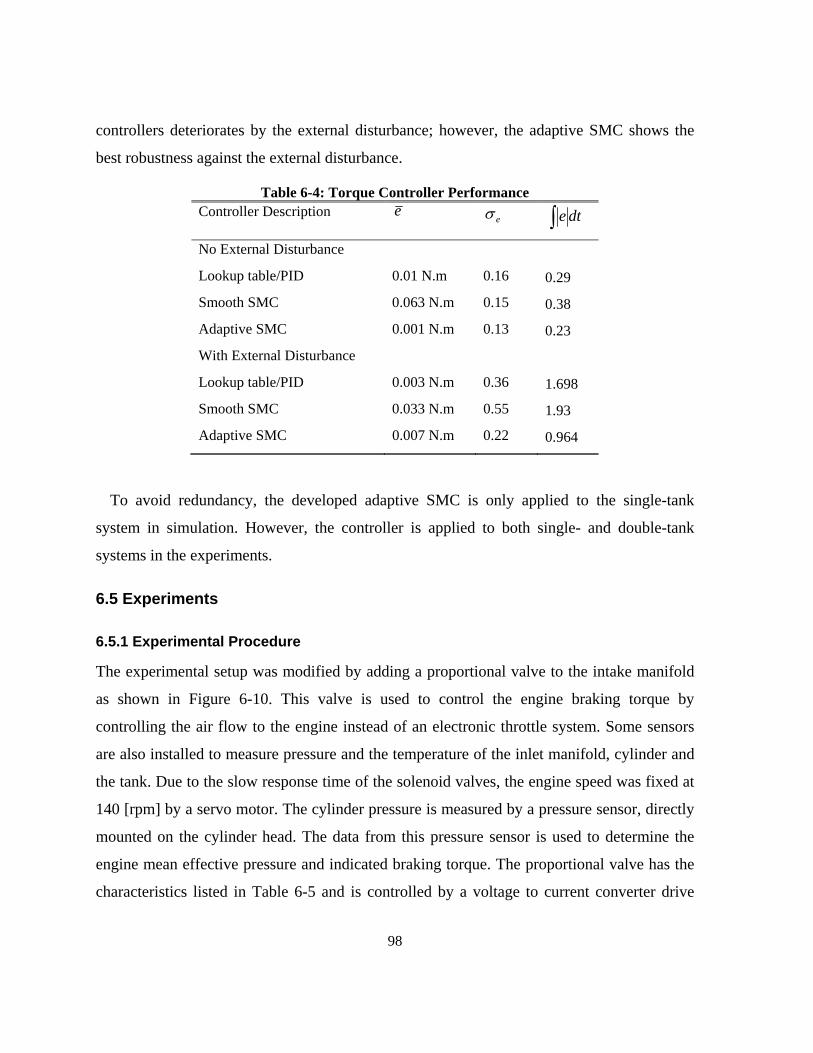
98
controllers deteriorates by the external disturbance; however, the adaptive SMC shows the
best robustness against the external disturbance.
Table 6-4: Torque Controller Performance Controller Description e
eσ ∫ dte
No External Disturbance
Lookup table/PID 0.01 N.m 0.16 0.29
Smooth SMC 0.063 N.m 0.15 0.38
Adaptive SMC 0.001 N.m 0.13 0.23
With External Disturbance
Lookup table/PID 0.003 N.m 0.36 1.698
Smooth SMC 0.033 N.m 0.55 1.93
Adaptive SMC 0.007 N.m 0.22 0.964
To avoid redundancy, the developed adaptive SMC is only applied to the single-tank
system in simulation. However, the controller is applied to both single- and double-tank
systems in the experiments.
6.5 Experiments
6.5.1 Experimental Procedure
The experimental setup was modified by adding a proportional valve to the intake manifold
as shown in Figure 6-10. This valve is used to control the engine braking torque by
controlling the air flow to the engine instead of an electronic throttle system. Some sensors
are also installed to measure pressure and the temperature of the inlet manifold, cylinder and
the tank. Due to the slow response time of the solenoid valves, the engine speed was fixed at
140 [rpm] by a servo motor. The cylinder pressure is measured by a pressure sensor, directly
mounted on the cylinder head. The data from this pressure sensor is used to determine the
engine mean effective pressure and indicated braking torque. The proportional valve has the
characteristics listed in Table 6-5 and is controlled by a voltage to current converter drive
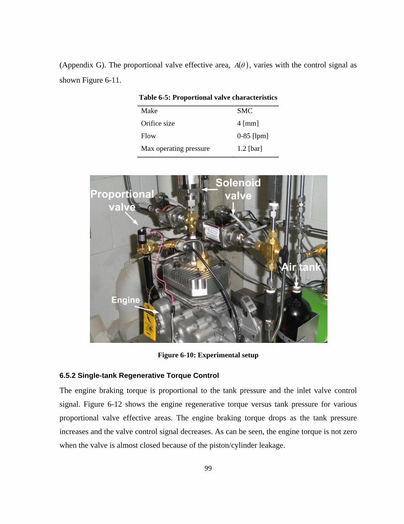
99
(Appendix G). The proportional valve effective area, ( )θA , varies with the control signal as
shown Figure 6-11.
Table 6-5: Proportional valve characteristics
Make SMC
Orifice size 4 [mm]
Flow 0-85 [lpm]
Max operating pressure 1.2 [bar]
Figure 6-10: Experimental setup
6.5.2 Single-tank Regenerative Torque Control
The engine braking torque is proportional to the tank pressure and the inlet valve control
signal. Figure 6-12 shows the engine regenerative torque versus tank pressure for various
proportional valve effective areas. The engine braking torque drops as the tank pressure
increases and the valve control signal decreases. As can be seen, the engine torque is not zero
when the valve is almost closed because of the piston/cylinder leakage.
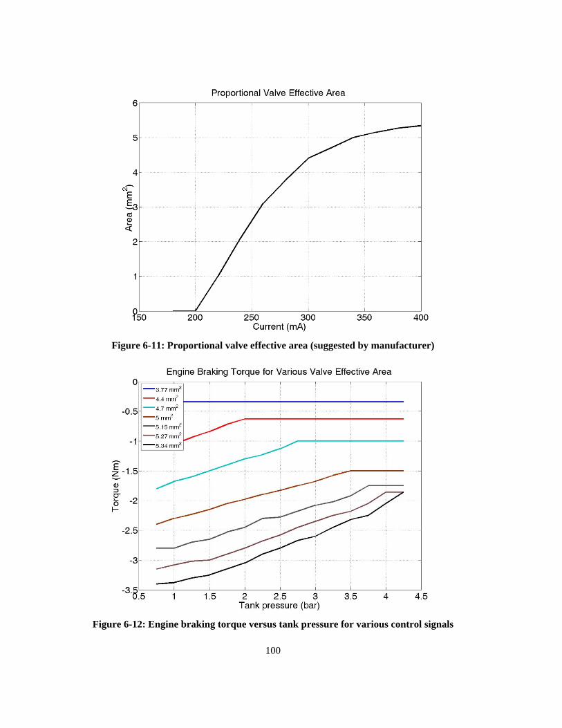
100
Figure 6-11: Proportional valve effective area (suggested by manufacturer)
Figure 6-12: Engine braking torque versus tank pressure for various control signals
101
In order to apply the adaptive SMC to the system, 1g and 2g in Eq.(6-12) are required. To
define these parameters engine volumetric efficiency maps, along with the online
measurement of the manifold pressure are required. However, since the flow to the engine
and to the tank cannot be measured in the available test bed, the volumetric efficiency maps
cannot be obtained. In addition, the pressure sensor mounted on the inlet manifold did not
show a meaningful pressure offset form atmospheric pressure which is mainly because of the
low engine speed. As a result, parameters required for defining 1g and 2g could not be
measured or identified. As a result, 1g and 2g were identified directly by measuring engineT& at
various operating points by the least square method (more details in Appendix H).
Three different controllers, adaptive SMC, smooth SMC and a PI controller are tuned and
used for the engine torque control. It is noteworthy that ASMC was tuned after only 4 trials;
however, PI and smooth SMC were tuned after 16 and 30 trials respectively. Controllers’
parameters are listed in Table 6-6.
Figure 6-13 shows the closed-loop tracking performance of the controllers. All the
controllers show satisfactory performances, however, ASMC and PI have the best tracking
performance as they track the desired torque within 5% (Figure 6-14), despite the continuous
change in the tank pressure and unfiltered sensor noises (Figure 6-15). For smooth SMC, the
overshoot is about 7%, however, the performance deteriorates with time and the steady state
error rises to about 13%.
Settling time for ASMC and PI is about 5 seconds (about 11 engine cycles) which is
mainly due to the slow engine speed (140 [rpm]). Figure 6-16 shows the actuator control
signal for ASMC controller. As can be seen, chattering is removed from the control signal
employing ASMC. The closed-loop performances of the three controllers are listed in Table
6-7.
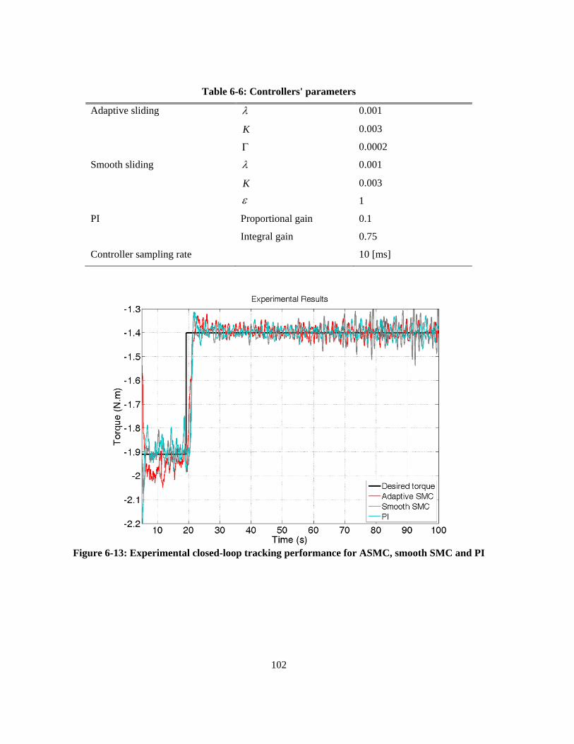
102
Table 6-6: Controllers' parameters
Adaptive sliding λ 0.001
K 0.003
Γ 0.0002
Smooth sliding λ 0.001
K 0.003
ε 1
PI Proportional gain 0.1
Integral gain 0.75
Controller sampling rate 10 [ms]
Figure 6-13: Experimental closed-loop tracking performance for ASMC, smooth SMC and PI
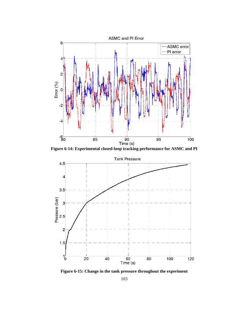
103
Figure 6-14: Experimental closed-loop tracking performance for ASMC and PI
Figure 6-15: Change in the tank pressure throughout the experiment
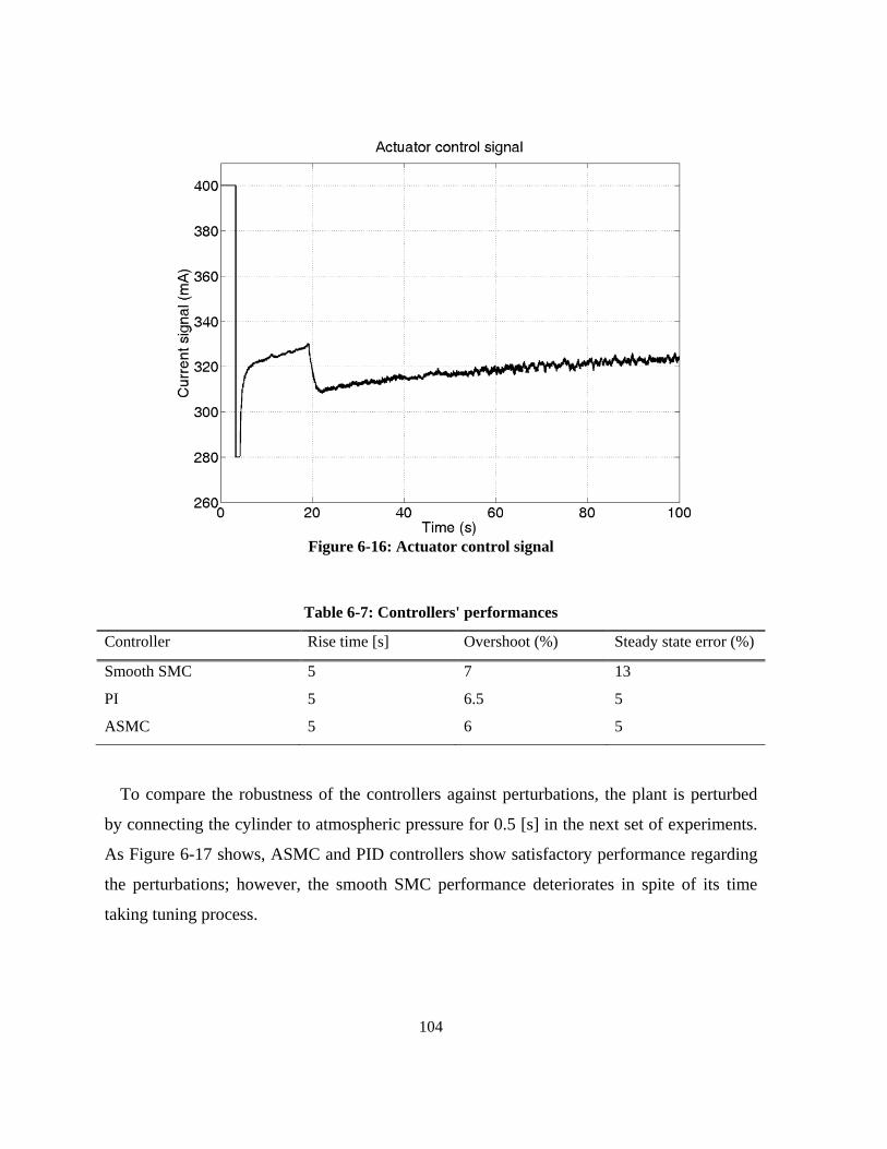
104
Figure 6-16: Actuator control signal
Table 6-7: Controllers' performances
Controller Rise time [s] Overshoot (%) Steady state error (%)
Smooth SMC 5 7 13
PI 5 6.5 5
ASMC 5 6 5
To compare the robustness of the controllers against perturbations, the plant is perturbed
by connecting the cylinder to atmospheric pressure for 0.5 [s] in the next set of experiments.
As Figure 6-17 shows, ASMC and PID controllers show satisfactory performance regarding
the perturbations; however, the smooth SMC performance deteriorates in spite of its time
taking tuning process.
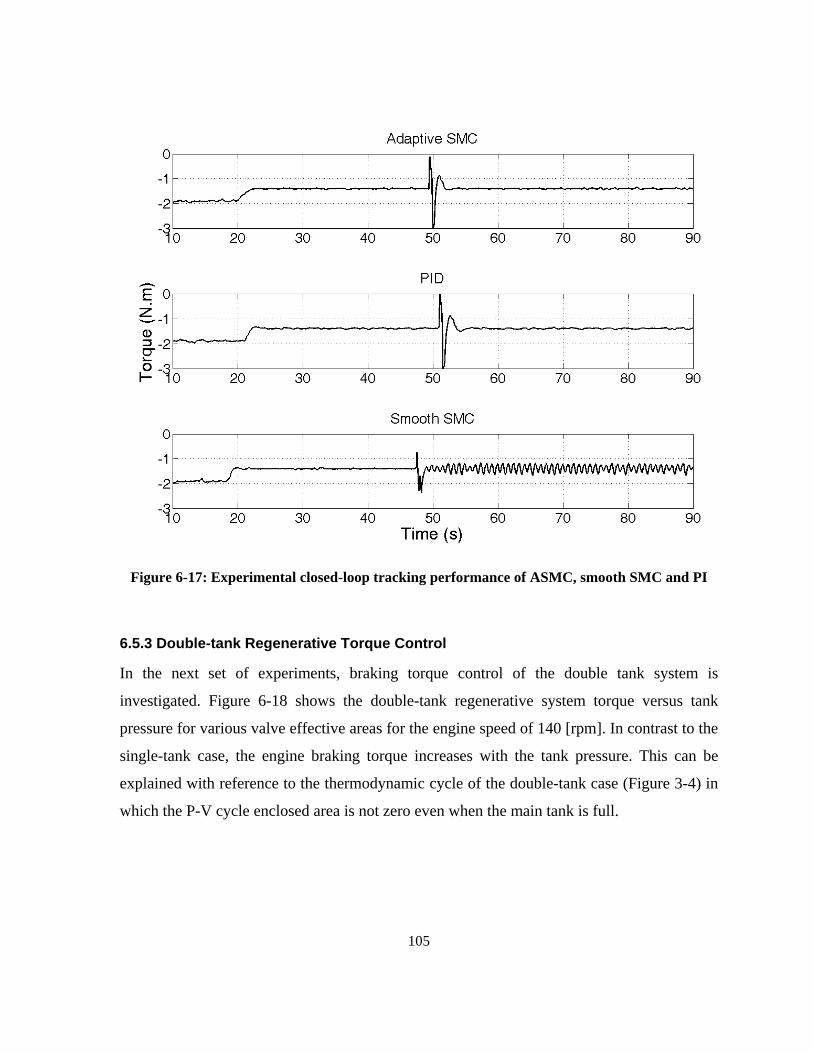
105
Figure 6-17: Experimental closed-loop tracking performance of ASMC, smooth SMC and PI
6.5.3 Double-tank Regenerative Torque Control
In the next set of experiments, braking torque control of the double tank system is
investigated. Figure 6-18 shows the double-tank regenerative system torque versus tank
pressure for various valve effective areas for the engine speed of 140 [rpm]. In contrast to the
single-tank case, the engine braking torque increases with the tank pressure. This can be
explained with reference to the thermodynamic cycle of the double-tank case (Figure 3-4) in
which the P-V cycle enclosed area is not zero even when the main tank is full.
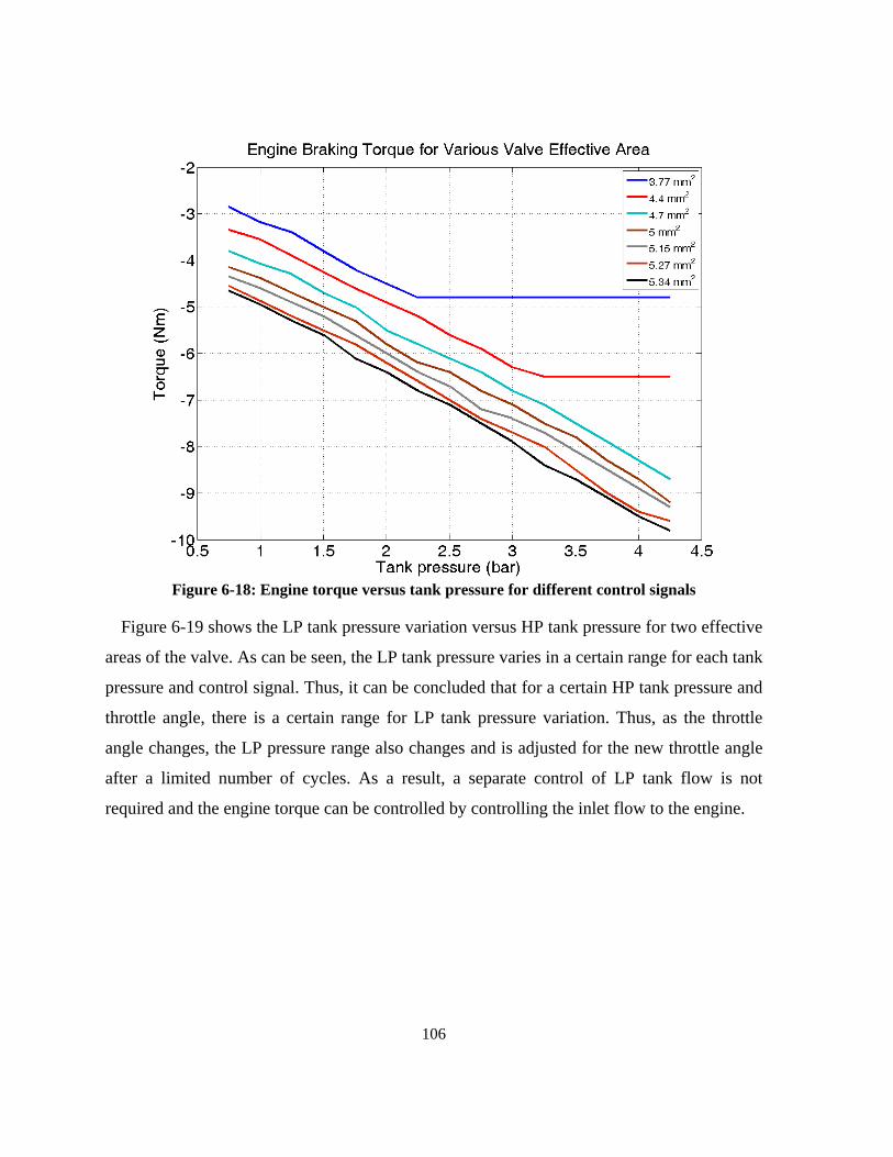
106
Figure 6-18: Engine torque versus tank pressure for different control signals
Figure 6-19 shows the LP tank pressure variation versus HP tank pressure for two effective
areas of the valve. As can be seen, the LP tank pressure varies in a certain range for each tank
pressure and control signal. Thus, it can be concluded that for a certain HP tank pressure and
throttle angle, there is a certain range for LP tank pressure variation. Thus, as the throttle
angle changes, the LP pressure range also changes and is adjusted for the new throttle angle
after a limited number of cycles. As a result, a separate control of LP tank flow is not
required and the engine torque can be controlled by controlling the inlet flow to the engine.
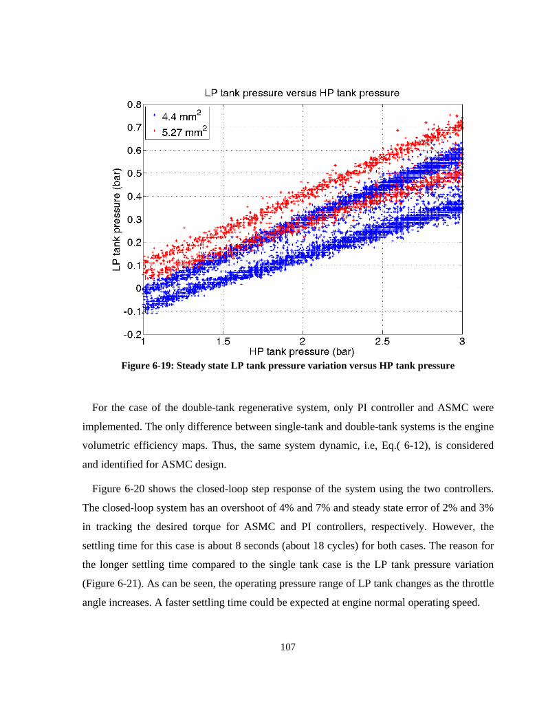
107
Figure 6-19: Steady state LP tank pressure variation versus HP tank pressure
For the case of the double-tank regenerative system, only PI controller and ASMC were
implemented. The only difference between single-tank and double-tank systems is the engine
volumetric efficiency maps. Thus, the same system dynamic, i.e, Eq.( 6-12), is considered
and identified for ASMC design.
Figure 6-20 shows the closed-loop step response of the system using the two controllers.
The closed-loop system has an overshoot of 4% and 7% and steady state error of 2% and 3%
in tracking the desired torque for ASMC and PI controllers, respectively. However, the
settling time for this case is about 8 seconds (about 18 cycles) for both cases. The reason for
the longer settling time compared to the single tank case is the LP tank pressure variation
(Figure 6-21). As can be seen, the operating pressure range of LP tank changes as the throttle
angle increases. A faster settling time could be expected at engine normal operating speed.
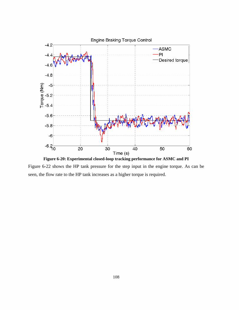
108
Figure 6-20: Experimental closed-loop tracking performance for ASMC and PI
Figure 6-22 shows the HP tank pressure for the step input in the engine torque. As can be
seen, the flow rate to the HP tank increases as a higher torque is required.
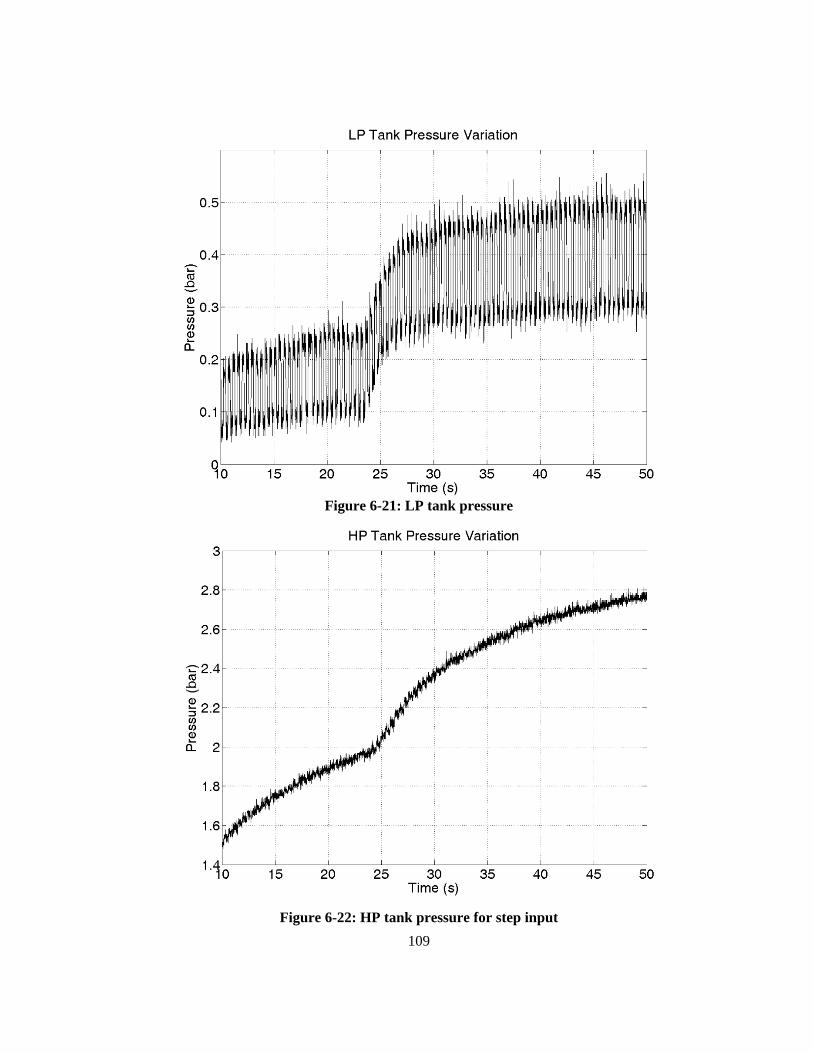
109
Figure 6-21: LP tank pressure
Figure 6-22: HP tank pressure for step input
110
6.6 Summary
In this chapter, a throttle-based regenerative braking torque control for air hybrid engines was
developed. A new mean value model for the engine during braking was derived and an
adaptive sliding mode was implemented for this particular application. The robustness and
performance of the controller was investigated and compared using simulation and
experiments with that of a high-gain PID and a model-based smooth sliding mode controller.
The experimental results showed that a throttle-based controller could be used efficiently to
regulate the regenerative braking torque in air hybrid engines.
111
Chapter 7 Drive Cycle Simulations
7.1 Background
An air hybrid vehicle uses two energy sources for propulsion: pressurized air and fossil fuel.
The air hybrid vehicle powertrain also has different modes of operation while accelerating
and braking. In practice, the performance of a hybrid engine is highly dependent on the
power management strategy for mode-schedule planning. Therefore, a supervisory control or
power management strategy should be designed to choose between the different modes of
operation. There are many studies in the literature addressing power management strategies
in hybrid vehicles. Typically, heuristic controllers are employed for power management in
vehicles.
In this chapter, the optimal power management strategy using Dynamic Programming (DP)
to minimize the vehicle fuel consumption for both the single and double-tank hybrid engines
are studied and compared. This study is conducted for two standard drive cycles.
7.1.1 Dynamic Programming
Dynamic programming can be applied to the following discrete dynamic systems [11]:
),,(1 kkk xFx α=+ 7-1
where { }ik xxXx ,...,1=∈ and { }jk ααα ,...,1=Α∈ are the system state and control action
respectively ( k is the step index) to find the optimal set of control actions that minimizes the
cost function, ( )0xΩ , subjected to both state and control action constraints. The solution to
this DP problem is the set of control actions, { }1210 ,...,,, −=Α fαααα , that minimizes the cost
function such that:
( ) ( ) .min 00 xxAoptimum Ω=Ω 7-2
112
The notion A
min is used to indicate the minimum of a function taken over all the possible
values of the variable A . The cost function for the discrete dynamic system (7-1) is defined
as [11]:
( ) ( ) ( ).,1
00 ∑
−
=
+=Ωf
kkkkff xxx αππ 7-3
In the above equation, ( )ff xπ is the cost associated with the final state and is usually set to
impose the constraint on the state final value and ( )kkk x απ , is the cost of applying kα at kx .
The DP method is applied backward in time, and is most useful for offline optimization
where the final state of the system is known a priori. Figure 7-1, shows how the method can
be applied to a system that is discretized both in space and time. The idea is to start from the
final states and define the cost associated with each final state of the system. A high cost is
assigned to those final states that are unlikely to occur or are constrained. Consequently, the
associated cost to each of the final states is defined as:
( ) ( ) ,if
if xx π=Ω 7-4
where ifx is the ith state at ft . Once the cost associated with each final state is determined,
the solution continues backward in time by calculating ( ) ,1ifx−
Ω as follows:
( ) ( ) ( )( ).,,min 11111jf
ifoptimum
jf
ifj
ifoptimum xFxx −−−−−
Ω+=Ω ααπ 7-5
Figure 7-1 shows the case where { }211 ,ααα ∈−f , and the two control actions, 1α and 2α that
can be applied to ifx 1− at 1−ft , take the system to ( )1
11 ,−−
= fif
if xFx α and ( )2
11 ,−− f
ifxF α at 1−ft .
In this case, the optimum cost associated with ifx 1− is expressed as:
( ) ( ) ( ) ( ) ( )( )( ) .,,,,min 211
211
1111 −−−−−−−
Ω+Ω+=Ω fifoptimumf
if
ifoptimumf
if
ifoptimum xFxxxx ααπαπ 7-6
Since the space is discritized in space, ( )211 ,−− f
ifxF α is not associated with any state. Thus,
( )( )211 , −−
Ω fifoptimum uxF should be calculated by interpolating ( )1−Ω i
foptimum x and ( )2−Ω ifoptimum x .
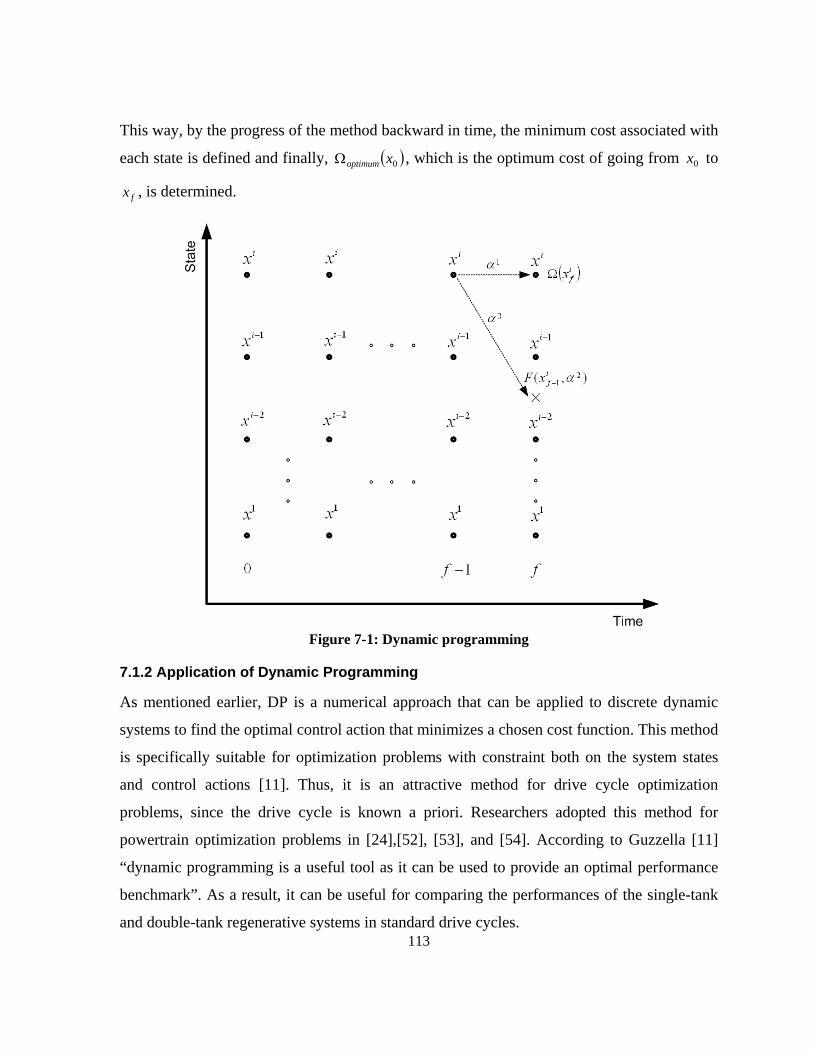
113
This way, by the progress of the method backward in time, the minimum cost associated with
each state is defined and finally, ( )0xoptimumΩ , which is the optimum cost of going from 0x to
fx , is determined.
Figure 7-1: Dynamic programming
7.1.2 Application of Dynamic Programming
As mentioned earlier, DP is a numerical approach that can be applied to discrete dynamic
systems to find the optimal control action that minimizes a chosen cost function. This method
is specifically suitable for optimization problems with constraint both on the system states
and control actions [11]. Thus, it is an attractive method for drive cycle optimization
problems, since the drive cycle is known a priori. Researchers adopted this method for
powertrain optimization problems in [24],[52], [53], and [54]. According to Guzzella [11]
“dynamic programming is a useful tool as it can be used to provide an optimal performance
benchmark”. As a result, it can be useful for comparing the performances of the single-tank
and double-tank regenerative systems in standard drive cycles.
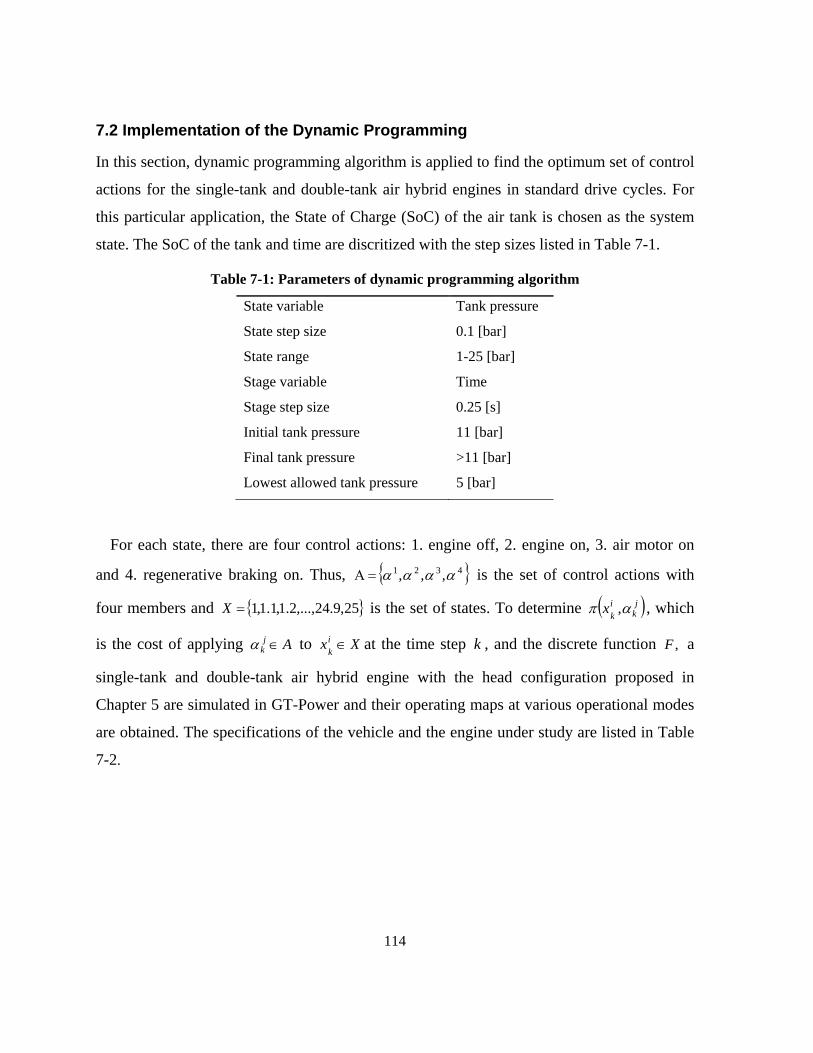
114
7.2 Implementation of the Dynamic Programming
In this section, dynamic programming algorithm is applied to find the optimum set of control
actions for the single-tank and double-tank air hybrid engines in standard drive cycles. For
this particular application, the State of Charge (SoC) of the air tank is chosen as the system
state. The SoC of the tank and time are discritized with the step sizes listed in Table 7-1.
Table 7-1: Parameters of dynamic programming algorithm
State variable Tank pressure
State step size 0.1 [bar]
State range 1-25 [bar]
Stage variable Time
Stage step size 0.25 [s]
Initial tank pressure 11 [bar]
Final tank pressure >11 [bar]
Lowest allowed tank pressure 5 [bar]
For each state, there are four control actions: 1. engine off, 2. engine on, 3. air motor on
and 4. regenerative braking on. Thus, { }4321 ,,, αααα=Α is the set of control actions with
four members and { }25,9.24,...,2.1,1.1,1=X is the set of states. To determine ( )jk
ikx απ , , which
is the cost of applying Ajk ∈α to Xxi
k ∈ at the time step k , and the discrete function ,F a
single-tank and double-tank air hybrid engine with the head configuration proposed in
Chapter 5 are simulated in GT-Power and their operating maps at various operational modes
are obtained. The specifications of the vehicle and the engine under study are listed in Table
7-2.
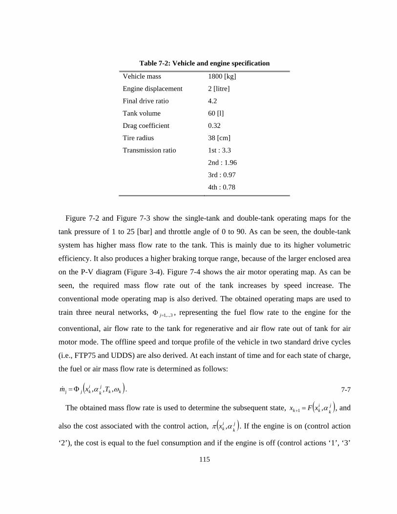
115
Table 7-2: Vehicle and engine specification
Vehicle mass 1800 [kg]
Engine displacement 2 [litre]
Final drive ratio 4.2
Tank volume 60 [l]
Drag coefficient 0.32
Tire radius 38 [cm]
Transmission ratio 1st : 3.3
2nd : 1.96
3rd : 0.97
4th : 0.78
Figure 7-2 and Figure 7-3 show the single-tank and double-tank operating maps for the
tank pressure of 1 to 25 [bar] and throttle angle of 0 to 90. As can be seen, the double-tank
system has higher mass flow rate to the tank. This is mainly due to its higher volumetric
efficiency. It also produces a higher braking torque range, because of the larger enclosed area
on the P-V diagram (Figure 3-4). Figure 7-4 shows the air motor operating map. As can be
seen, the required mass flow rate out of the tank increases by speed increase. The
conventional mode operating map is also derived. The obtained operating maps are used to
train three neural networks, 3,..,1=Φ j , representing the fuel flow rate to the engine for the
conventional, air flow rate to the tank for regenerative and air flow rate out of tank for air
motor mode. The offline speed and torque profile of the vehicle in two standard drive cycles
(i.e., FTP75 and UDDS) are also derived. At each instant of time and for each state of charge,
the fuel or air mass flow rate is determined as follows:
( ) .,,,j kkjk
ikj Txm ωαΦ=& 7-7
The obtained mass flow rate is used to determine the subsequent state, ( )jk
ikk xFx α,1 =+ , and
also the cost associated with the control action, ( )jk
ikx απ , . If the engine is on (control action
‘2’), the cost is equal to the fuel consumption and if the engine is off (control actions ‘1’, ‘3’
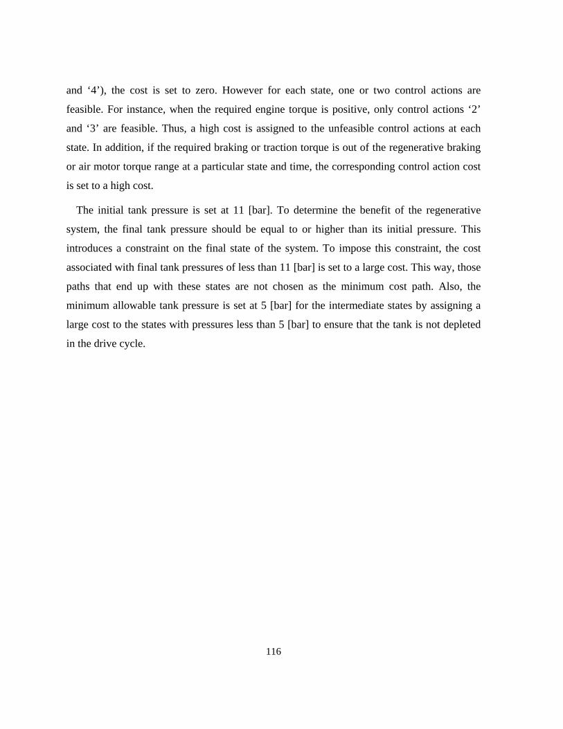
116
and ‘4’), the cost is set to zero. However for each state, one or two control actions are
feasible. For instance, when the required engine torque is positive, only control actions ‘2’
and ‘3’ are feasible. Thus, a high cost is assigned to the unfeasible control actions at each
state. In addition, if the required braking or traction torque is out of the regenerative braking
or air motor torque range at a particular state and time, the corresponding control action cost
is set to a high cost.
The initial tank pressure is set at 11 [bar]. To determine the benefit of the regenerative
system, the final tank pressure should be equal to or higher than its initial pressure. This
introduces a constraint on the final state of the system. To impose this constraint, the cost
associated with final tank pressures of less than 11 [bar] is set to a large cost. This way, those
paths that end up with these states are not chosen as the minimum cost path. Also, the
minimum allowable tank pressure is set at 5 [bar] for the intermediate states by assigning a
large cost to the states with pressures less than 5 [bar] to ensure that the tank is not depleted
in the drive cycle.
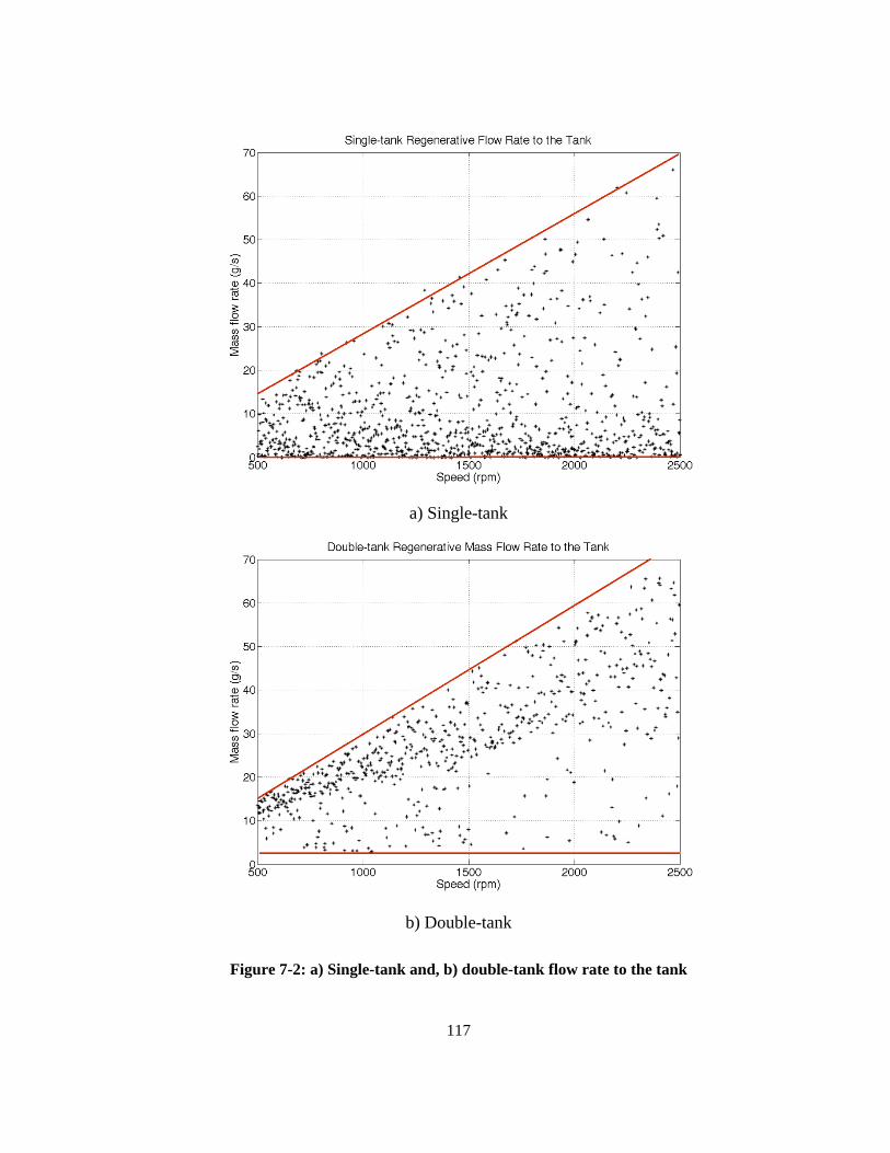
117
a) Single-tank
b) Double-tank
Figure 7-2: a) Single-tank and, b) double-tank flow rate to the tank
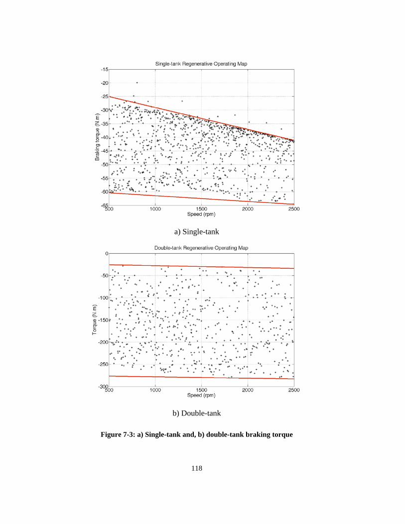
118
a) Single-tank
b) Double-tank
Figure 7-3: a) Single-tank and, b) double-tank braking torque
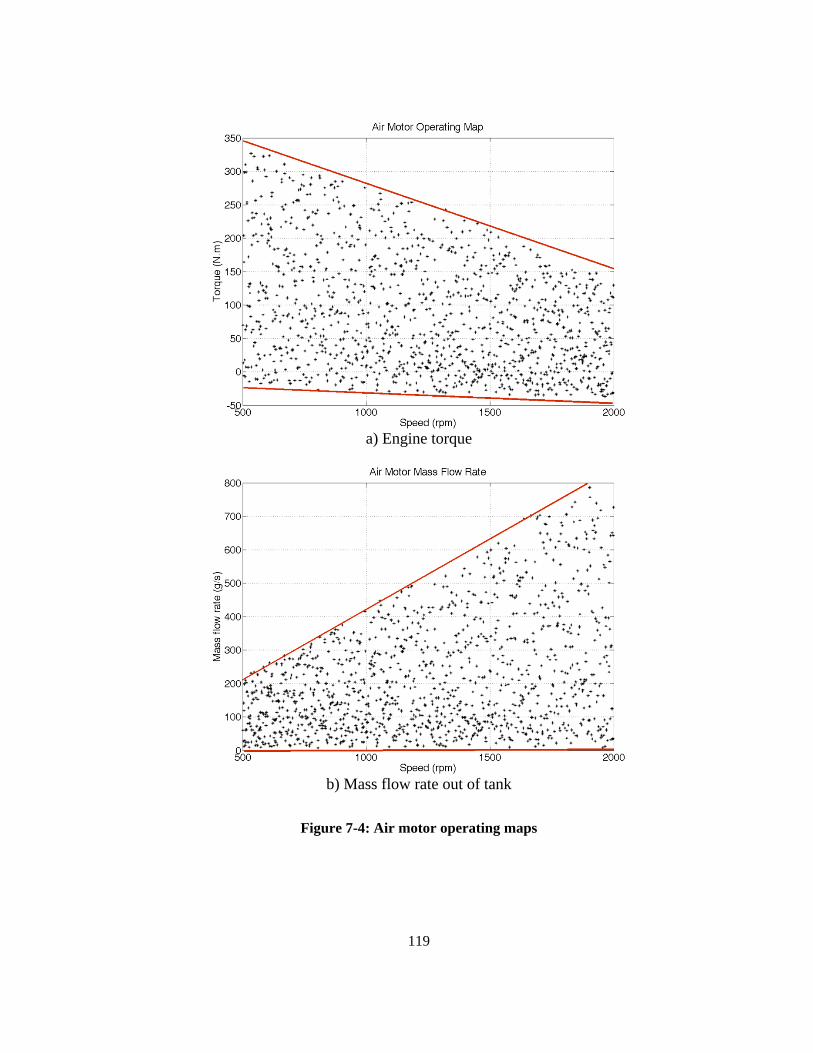
119
a) Engine torque
b) Mass flow rate out of tank
Figure 7-4: Air motor operating maps
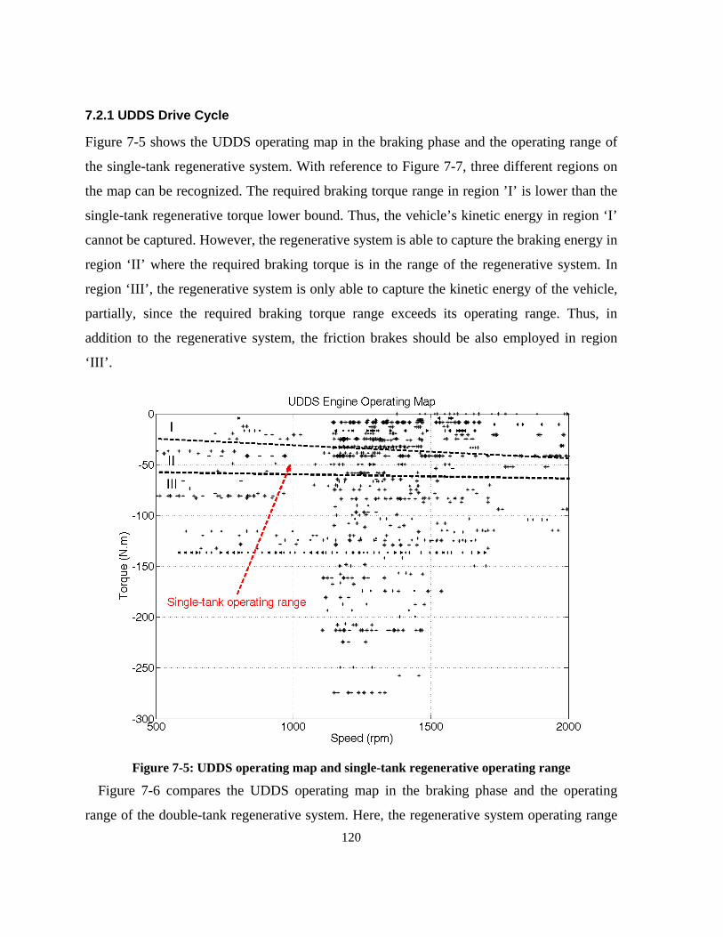
120
7.2.1 UDDS Drive Cycle
Figure 7-5 shows the UDDS operating map in the braking phase and the operating range of
the single-tank regenerative system. With reference to Figure 7-7, three different regions on
the map can be recognized. The required braking torque range in region ’I’ is lower than the
single-tank regenerative torque lower bound. Thus, the vehicle’s kinetic energy in region ‘I’
cannot be captured. However, the regenerative system is able to capture the braking energy in
region ‘II’ where the required braking torque is in the range of the regenerative system. In
region ‘III’, the regenerative system is only able to capture the kinetic energy of the vehicle,
partially, since the required braking torque range exceeds its operating range. Thus, in
addition to the regenerative system, the friction brakes should be also employed in region
‘III’.
Figure 7-5: UDDS operating map and single-tank regenerative operating range
Figure 7-6 compares the UDDS operating map in the braking phase and the operating
range of the double-tank regenerative system. Here, the regenerative system operating range
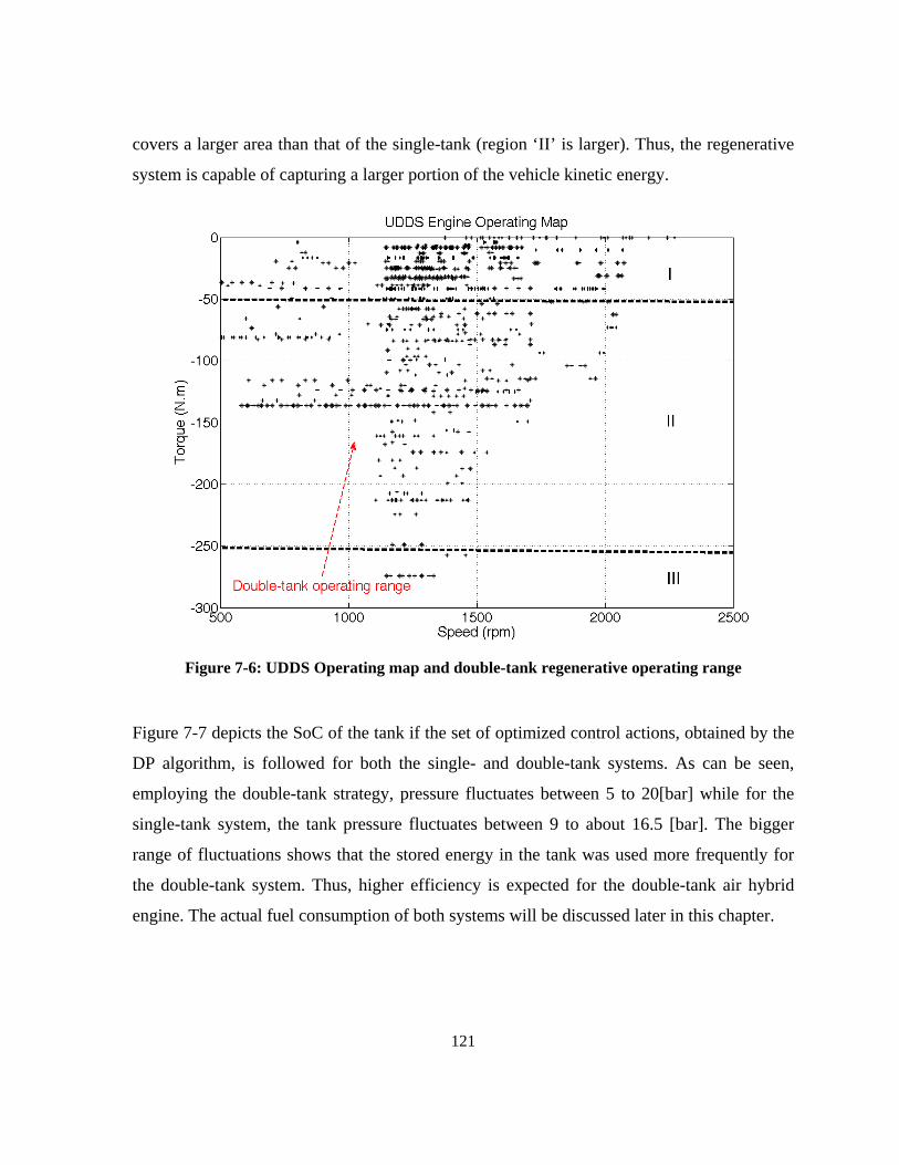
121
covers a larger area than that of the single-tank (region ‘II’ is larger). Thus, the regenerative
system is capable of capturing a larger portion of the vehicle kinetic energy.
Figure 7-6: UDDS Operating map and double-tank regenerative operating range
Figure 7-7 depicts the SoC of the tank if the set of optimized control actions, obtained by the
DP algorithm, is followed for both the single- and double-tank systems. As can be seen,
employing the double-tank strategy, pressure fluctuates between 5 to 20[bar] while for the
single-tank system, the tank pressure fluctuates between 9 to about 16.5 [bar]. The bigger
range of fluctuations shows that the stored energy in the tank was used more frequently for
the double-tank system. Thus, higher efficiency is expected for the double-tank air hybrid
engine. The actual fuel consumption of both systems will be discussed later in this chapter.
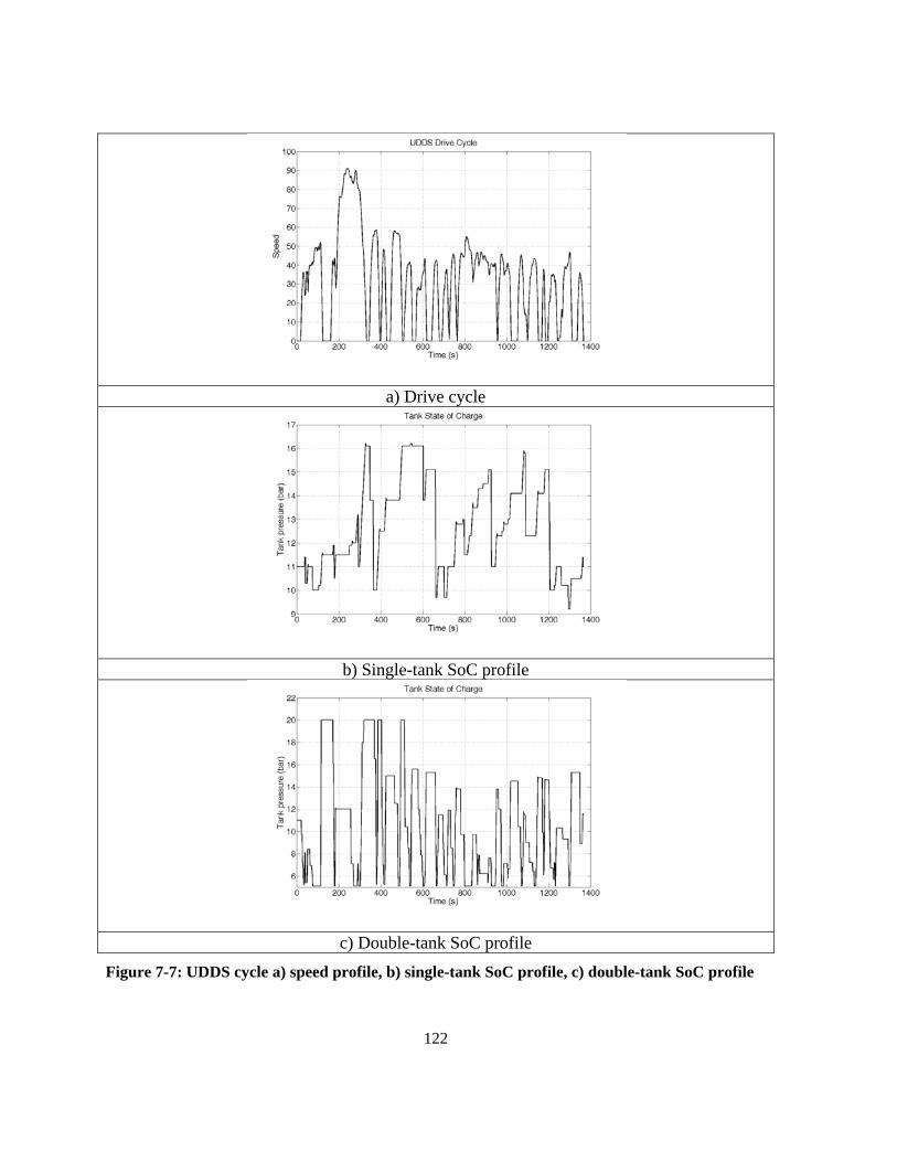
122
a) Drive cycle
b) Single-tank SoC profile
c) Double-tank SoC profile Figure 7-7: UDDS cycle a) speed profile, b) single-tank SoC profile, c) double-tank SoC profile
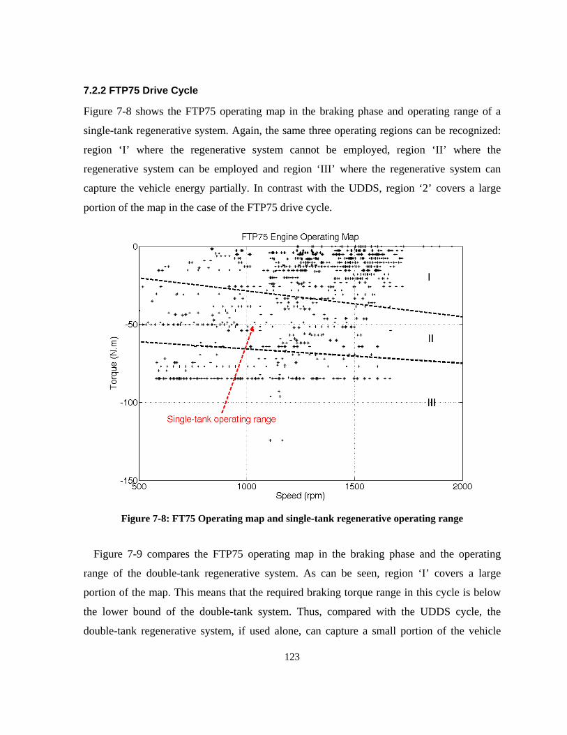
123
7.2.2 FTP75 Drive Cycle
Figure 7-8 shows the FTP75 operating map in the braking phase and operating range of a
single-tank regenerative system. Again, the same three operating regions can be recognized:
region ‘I’ where the regenerative system cannot be employed, region ‘II’ where the
regenerative system can be employed and region ‘III’ where the regenerative system can
capture the vehicle energy partially. In contrast with the UDDS, region ‘2’ covers a large
portion of the map in the case of the FTP75 drive cycle.
Figure 7-8: FT75 Operating map and single-tank regenerative operating range
Figure 7-9 compares the FTP75 operating map in the braking phase and the operating
range of the double-tank regenerative system. As can be seen, region ‘I’ covers a large
portion of the map. This means that the required braking torque range in this cycle is below
the lower bound of the double-tank system. Thus, compared with the UDDS cycle, the
double-tank regenerative system, if used alone, can capture a small portion of the vehicle
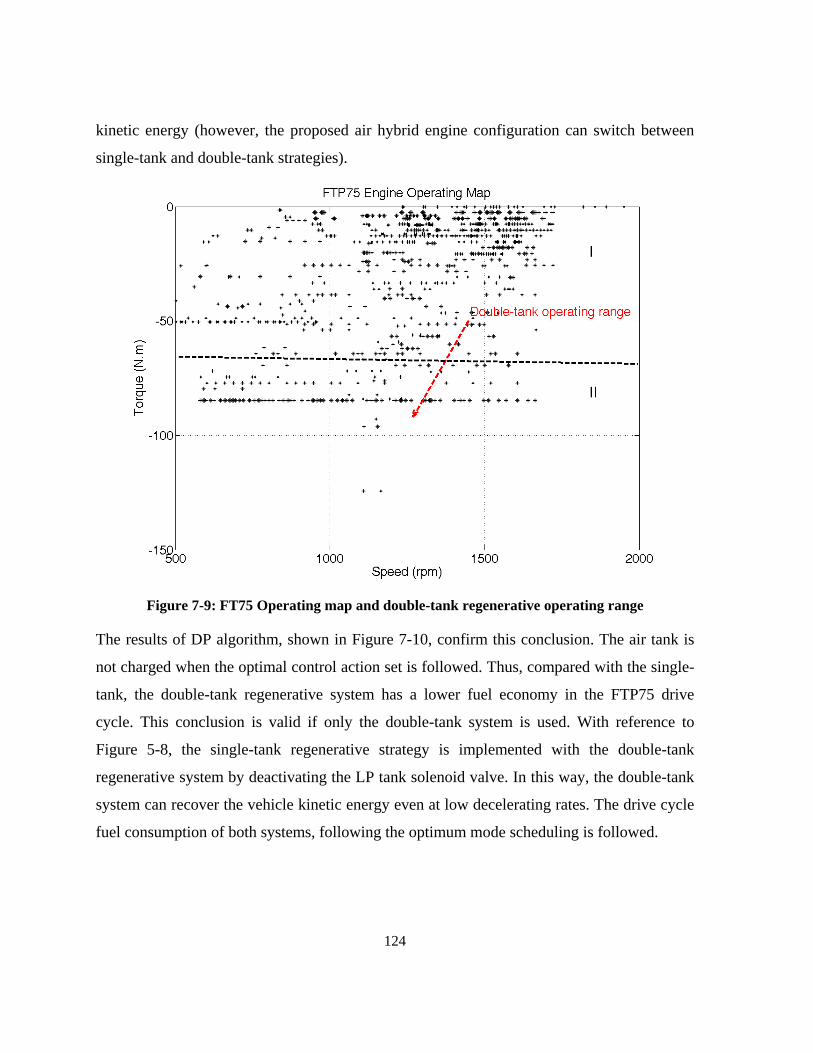
124
kinetic energy (however, the proposed air hybrid engine configuration can switch between
single-tank and double-tank strategies).
Figure 7-9: FT75 Operating map and double-tank regenerative operating range
The results of DP algorithm, shown in Figure 7-10, confirm this conclusion. The air tank is
not charged when the optimal control action set is followed. Thus, compared with the single-
tank, the double-tank regenerative system has a lower fuel economy in the FTP75 drive
cycle. This conclusion is valid if only the double-tank system is used. With reference to
Figure 5-8, the single-tank regenerative strategy is implemented with the double-tank
regenerative system by deactivating the LP tank solenoid valve. In this way, the double-tank
system can recover the vehicle kinetic energy even at low decelerating rates. The drive cycle
fuel consumption of both systems, following the optimum mode scheduling is followed.
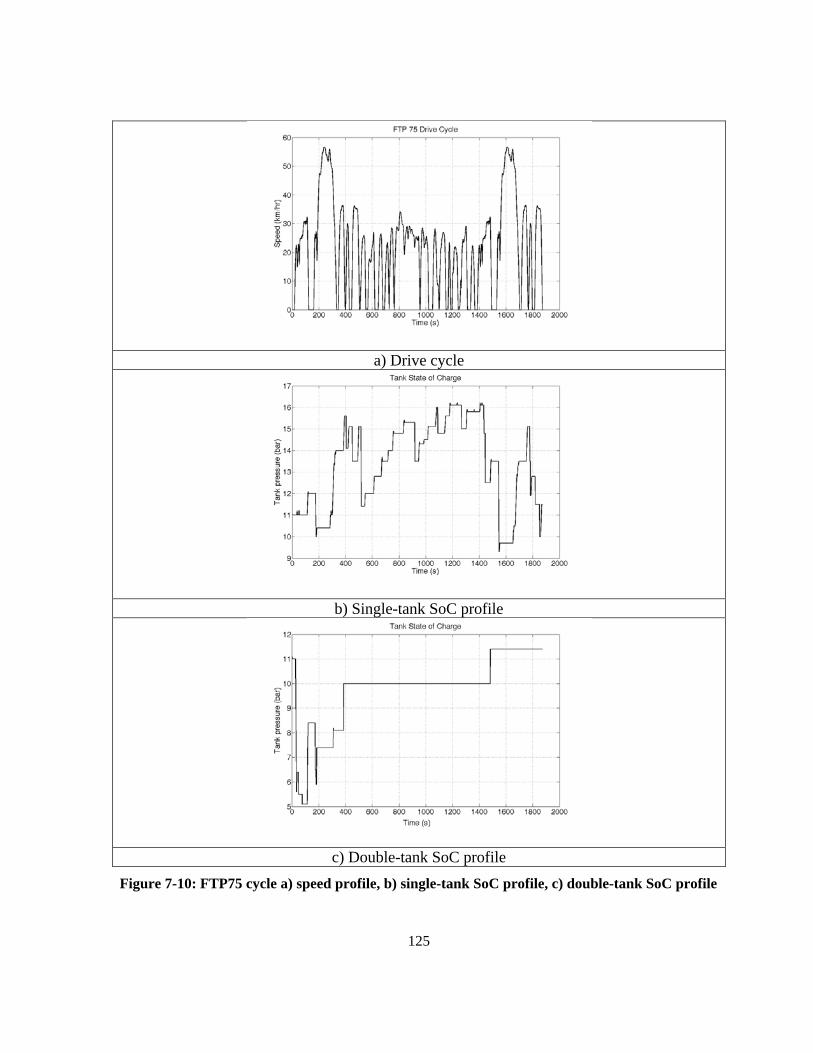
125
a) Drive cycle
b) Single-tank SoC profile
c) Double-tank SoC profile Figure 7-10: FTP75 cycle a) speed profile, b) single-tank SoC profile, c) double-tank SoC profile
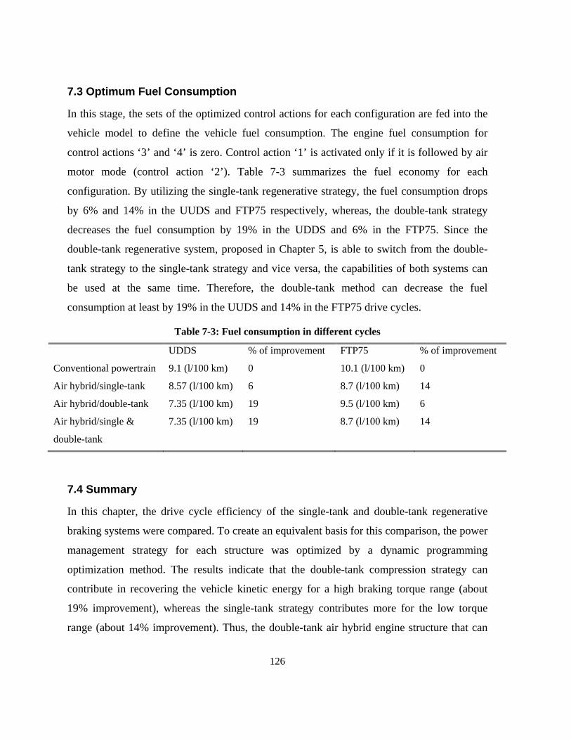
126
7.3 Optimum Fuel Consumption
In this stage, the sets of the optimized control actions for each configuration are fed into the
vehicle model to define the vehicle fuel consumption. The engine fuel consumption for
control actions ‘3’ and ‘4’ is zero. Control action ‘1’ is activated only if it is followed by air
motor mode (control action ‘2’). Table 7-3 summarizes the fuel economy for each
configuration. By utilizing the single-tank regenerative strategy, the fuel consumption drops
by 6% and 14% in the UUDS and FTP75 respectively, whereas, the double-tank strategy
decreases the fuel consumption by 19% in the UDDS and 6% in the FTP75. Since the
double-tank regenerative system, proposed in Chapter 5, is able to switch from the double-
tank strategy to the single-tank strategy and vice versa, the capabilities of both systems can
be used at the same time. Therefore, the double-tank method can decrease the fuel
consumption at least by 19% in the UUDS and 14% in the FTP75 drive cycles.
Table 7-3: Fuel consumption in different cycles
UDDS % of improvement FTP75 % of improvement
Conventional powertrain 9.1 (l/100 km) 0 10.1 (l/100 km) 0
Air hybrid/single-tank 8.57 (l/100 km) 6 8.7 (l/100 km) 14
Air hybrid/double-tank 7.35 (l/100 km) 19 9.5 (l/100 km) 6
Air hybrid/single &
double-tank
7.35 (l/100 km) 19 8.7 (l/100 km) 14
7.4 Summary
In this chapter, the drive cycle efficiency of the single-tank and double-tank regenerative
braking systems were compared. To create an equivalent basis for this comparison, the power
management strategy for each structure was optimized by a dynamic programming
optimization method. The results indicate that the double-tank compression strategy can
contribute in recovering the vehicle kinetic energy for a high braking torque range (about
19% improvement), whereas the single-tank strategy contributes more for the low torque
range (about 14% improvement). Thus, the double-tank air hybrid engine structure that can

127
implement both the single- and double-tank compression strategies can capture both low and
high braking torque ranges.
128
Chapter 8 Conclusions and Future Work
8.1 Summary of Contributions
In this thesis a new air hybrid engine with higher efficiency and lower complexity was
developed. It was shown in Chapter 3 that the storing capacity of a conventional, single-tank
regenerative air hybrid system was limited. Thus, a compression strategy based on using two
tanks was proposed to increase the energy storing capacity of the system during braking. The
double-tank compression strategy increases the volumetric efficiency of the engine during
braking, the system capacity in storing air mass, and the range of the braking torque
compared with the single-tank compression method. Although the efficiency of regenerative
braking system is dependent to the vehicle initial velocity, it was shown that the double-tank
strategy could lead to 28% energy recovery, whereas the single-tank system captures only
14% of the vehicle initial kinetic energy in a single braking event The double-tank strategy
was tested and compared experimentally with the single-tank regenerative system in Chapter
4. The experimental results confirmed the higher energy storing capacity of the double-tank
system.
A switchable cam-based valvetrain was proposed for implementing the air hybrid engine in
Chapter 5. Both single-tank and double-tank regenerative systems can be implemented by the
proposed configuration. One of the advantages of the proposed system is that the
regenerative braking torque can be controlled by the same electronic throttle used in the
traction torque control. The feasibility and performance of the proposed cam-based valvetrain
were shown through simulation and experiments.
The feasibility of engine braking torque control using the electronic throttle was shown in
Chapter 6. Since the engine is a highly non-linear system, the regenerative braking mean
value model was derived and an adaptive sliding mode controller was developed for this
particular application.
129
In Chapter 7, drive cycle efficiency of single-tank and double-tank regenerative braking
systems were compared. In order to create an equivalent basis for this comparison, the
optimized power management strategy for each method was obtained using the dynamic
programming. The results showed that the cam-based double-tank air hybrid engine can
improve the fuel economy by 19% in UDDS and 14% in FTP75 drive cycles. A higher fuel
economy could be expected if the air hybrid engine is run in supercharged mode and as a
result, a down-sized engine is used (34% in MVEG-95 drive cycle [24])
8.2 Publications Resulting from This Thesis
Several publications and a patent have resulted from this research as follows:
1. Fazeli A., Zeinali M., Khajepour A., ‘Application of Adaptive Sliding Mode Control
Regenerative Braking Torque Control’, IEEE/ASME Transactions on Mechatronics,
DOI 10.1109/TMECH.2011.2129525.
2. Fazeli A., Khajepour A., Devaud C., ‘A Novel Compression Strategy for Air Hybrid
Engines’, Journal of Applied Energy, 2011 doi:10.1016/j.apenergy.2011.03.008.
3. Fazeli A., Khajepour A., Devaud C., Pournazeri M., ‘Regenerative Braking Torque
Control of Air Hybrid Engines with Cam-Based Valvetrains’, Int. Journal of
Powertrains, 2010 (Accepted for publication).
4. Fazeli A., Khajepour A., Devaud C. and Pournazeri M., “A Novel Air Hybrid Engine
Configuration Utilizing Cam-based Valvetrain”, SAE World Congress & Exhibition
2011, paper# 2011-01-0871.
5. Fazeli A., Zeinali M., Khajepour A., Pournazeri M., “Air Hybrid Engine Torque
Control Using Adaptive Sliding Mode Control”, ASME International Mechanical
Engineering Congress and Exposition IMECE2010, November 12-18, 2010,
Vancouver, British Columbia, Canada, Paper# IMECE2010-38762.
6. Fazeli A., Khajepour A., Devaud C., Lashgarian N., “A New Air Hybrid Engine
Using Throttle Control”, SAE World Congress & Exhibition, Detroit, Michigan,
USA, 2009, Paper# 2009-01-1319.
130
7. Khajepour A., Fazeli A., Devaud C. and Azad N., ‘Air compression method and
apparatus’ PTC pending patent number: 090218-0028, 2010.
8.3 Suggestions for Future Work
In regards to the future work on air hybrid engines, the following directions are suggested:
1. Complete thermal analysis: Since the speed was low and engine was not fired in the
available setup, the temperature increase during compression was not significant. At
nominal engine temperature and speed ranges, the temperature rise due to the
compression is an important factor and should be investigated.
2. Full implementation of the switchable cam-based valvetrain: The switchable
valvetrain was not implemented using fixed valve timings in this thesis. A full
implementation is needed to study different engine operational modes and switching
between them at the nominal speed range of an engine.
3. Full implementation of the suggested air hybrid engine: Although the proposed
double-tank strategy was proven to have higher efficiency and a simpler valvetrain, it
needs to be implemented on a real engine.
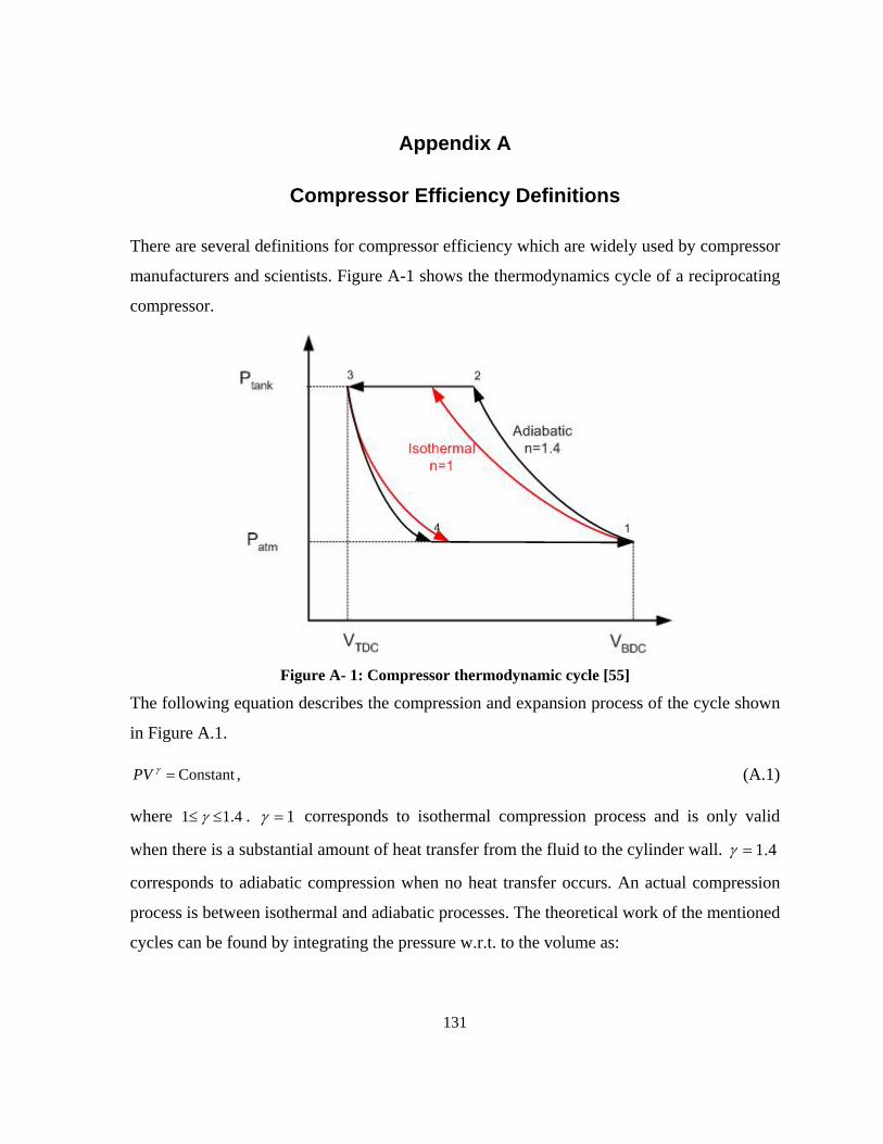
131
Appendix A
Compressor Efficiency Definitions
There are several definitions for compressor efficiency which are widely used by compressor
manufacturers and scientists. Figure A-1 shows the thermodynamics cycle of a reciprocating
compressor.
Figure A- 1: Compressor thermodynamic cycle [55]
The following equation describes the compression and expansion process of the cycle shown
in Figure A.1.
,Constant=γPV (A.1)
where 4.11 ≤≤ γ . 1=γ corresponds to isothermal compression process and is only valid
when there is a substantial amount of heat transfer from the fluid to the cylinder wall. 4.1=γ
corresponds to adiabatic compression when no heat transfer occurs. An actual compression
process is between isothermal and adiabatic processes. The theoretical work of the mentioned
cycles can be found by integrating the pressure w.r.t. to the volume as:
132
( ) .∫= dVVPW (A.2)
Theoretical power is also expressed by following relation:
.2
WW compressor
πω
=& (A.3)
Adiabatic power, adW& and isoW& are the theoretical compressor power if all the expansions
and compressions are assumed to be adiabatic or isothermal respectively. Actual power, actW&
, is also the measured power from an experimentally measured P-V curve. The
experimentally measured power to run the compressor is shaft power, shaftW& , and is expressed
as follows:
frictionactshaft WWW &&& += (A.4)
Based on the mentioned cycle and definitions, the following definitions for efficiency can be
derived:
Volumetric Efficiency:
The ratio of the volume actually pumped to the volume swept by the piston is volumetric
efficiency and, according to Figure A.1, is defined by the following relation:
31
41
VVVV
vol −−
=η (A.5)
The volumetric efficiency of a compressor is always less than one because of trapped gas in
the clearance volume, the imperfect nature of the valves and wall friction [56].
Adiabatic Efficiency:
Adiabatic efficiency is the ratio of adiabatic power to the actual power and is defined as
follows:
act
adadiabatic W
W&
&=η (A.6)
133
Isothermal Efficiency:
Isothermal efficiency is the ratio of isothermal power to the actual power and is defined as
follows:
act
isoiso W
W&
&=η (A.7)
Mechanical Efficiency:
Mechanical efficiency is the ratio of actual power to the shaft power and is defined as
follows:
shaft
actmech W
W&
&=η (A.8)
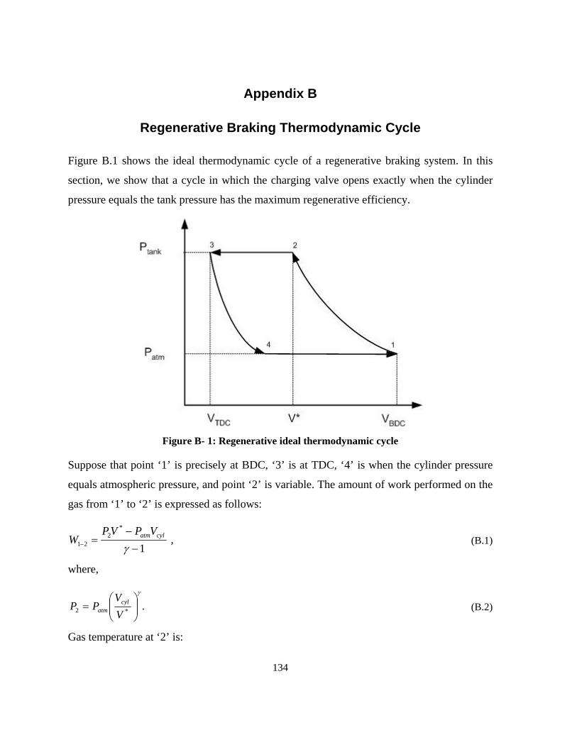
134
Appendix B
Regenerative Braking Thermodynamic Cycle
Figure B.1 shows the ideal thermodynamic cycle of a regenerative braking system. In this
section, we show that a cycle in which the charging valve opens exactly when the cylinder
pressure equals the tank pressure has the maximum regenerative efficiency.
Figure B- 1: Regenerative ideal thermodynamic cycle
Suppose that point ‘1’ is precisely at BDC, ‘3’ is at TDC, ‘4’ is when the cylinder pressure
equals atmospheric pressure, and point ‘2’ is variable. The amount of work performed on the
gas from ‘1’ to ‘2’ is expressed as follows:
,1
*2
21 −
−=− γ
cylatmVPVPW (B.1)
where,
.*2
γ
⎟⎟⎠
⎞⎜⎜⎝
⎛=
VV
PP cylatm (B.2)
Gas temperature at ‘2’ is:
135
.1
*2
−
⎟⎟⎠
⎞⎜⎜⎝
⎛=
γ
υυVVcyl
atm (B.3)
Work between ‘2’ and ‘3’ is expressed by:
,1
**2tank3
32 −
−⎟⎟⎠
⎞⎜⎜⎝
⎛+
=− γ
VPVCV
PW r
cyl
(B.4)
where,
,tank
*tanktank2
**
2 VVPVPVP
++
= (B.5)
and,
.tank
*tank*
23
γ
⎟⎟⎟⎟⎟
⎠
⎞
⎜⎜⎜⎜⎜
⎝
⎛
+
+=
r
cyl
CV
V
VVPP (B.6)
Temperature at point ‘3’ is:
,
1
tank
*tank*
23
−
⎟⎟⎟⎟⎟
⎠
⎞
⎜⎜⎜⎜⎜
⎝
⎛
+
+=
γ
υυ
r
cyl
CV
V
VV (B.7)
where, assuming ideal mixing of gases we have:
( ) .1
tank
tanktank
2
*2*
tank*
2*2
−
⎟⎟⎠
⎞⎜⎜⎝
⎛++=
υυυ VPVPVVP (B.8)
Work between ‘3’ and ‘4’ is defined by:
,1
34
43 −
−=− γ
r
cylatm C
VPVP
W (B.9)
where,
136
.
1
34
γ
⎟⎟⎠
⎞⎜⎜⎝
⎛=
atmr
cyl
PP
CV
V (B.10)
Work between ‘4’ and ‘1’ is also defined by:
( ).1414 VVPW atm −=− (B.11)
The total work of the cycle can be defined by:
.41433221 −−−− +++= WWWWWtot (B.12)
The amount of mass stored in the tank is:
.1
3
3
airr
cyl
atm
cylatminduced MC
VPVP
Rm
⎟⎟⎟⎟⎟
⎠
⎞
⎜⎜⎜⎜⎜
⎝
⎛
−=υυ
(B.13)
Now, in order to maximize the cycle efficiency, the following equation should be solved:
.0=tot
induced
dWdm
(B.14)
Using MAPLE, the solution of the above equation with respect to *V is found to be:
.
1
tan
*γ
⎟⎟⎠
⎞⎜⎜⎝
⎛=
k
atmcyl P
PVV (B.15)
The result shows that in order to have maximum efficiency of a regenerative cycle, the
charging valve should open when the cylinder pressure equals the tank pressure.
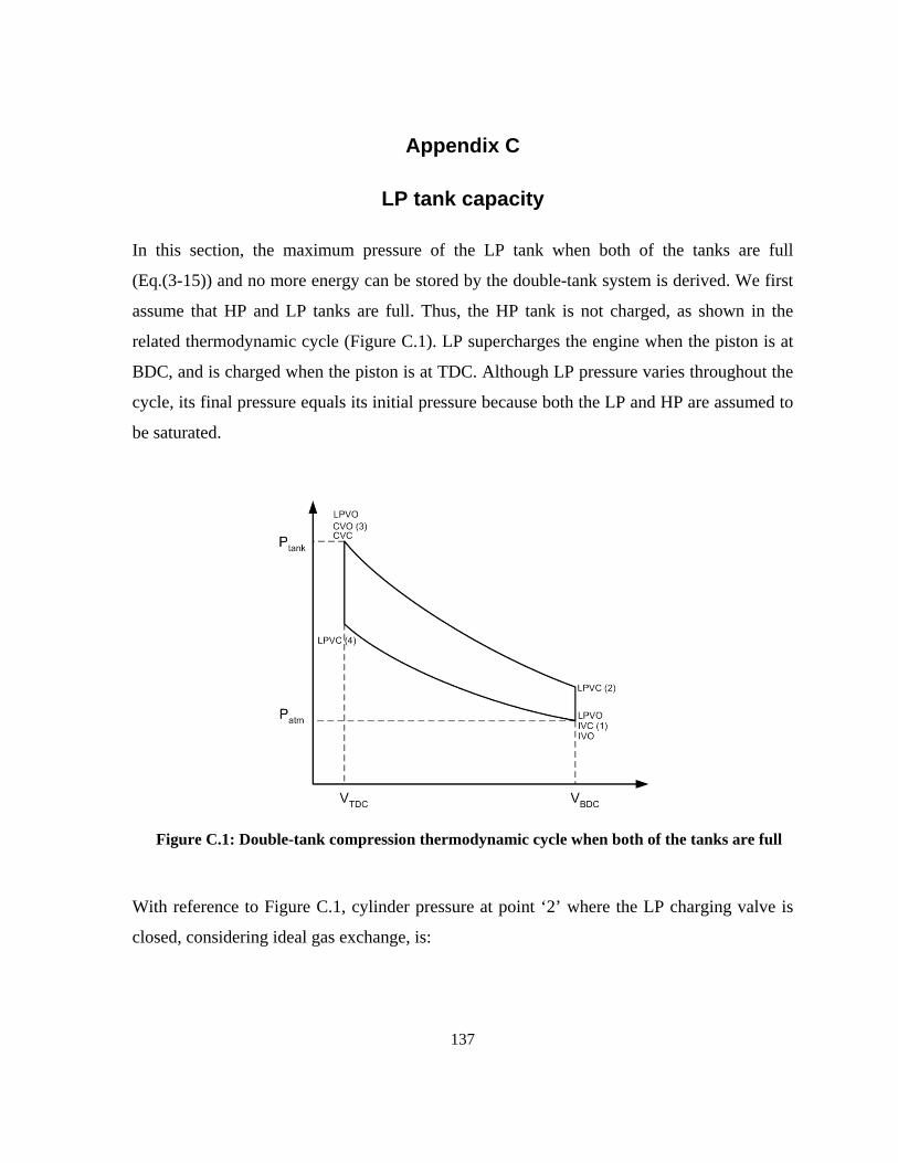
137
Appendix C
LP tank capacity
In this section, the maximum pressure of the LP tank when both of the tanks are full
(Eq.(3-15)) and no more energy can be stored by the double-tank system is derived. We first
assume that HP and LP tanks are full. Thus, the HP tank is not charged, as shown in the
related thermodynamic cycle (Figure C.1). LP supercharges the engine when the piston is at
BDC, and is charged when the piston is at TDC. Although LP pressure varies throughout the
cycle, its final pressure equals its initial pressure because both the LP and HP are assumed to
be saturated.
Figure C.1: Double-tank compression thermodynamic cycle when both of the tanks are full
With reference to Figure C.1, cylinder pressure at point ‘2’ where the LP charging valve is
closed, considering ideal gas exchange, is:
138
.2LPcyl
LPLPcylatm
VVVPVP
P+
+= (C.1)
Since the LP tank should be cooled down, its initial temperature is assumed to be equal to
the atmospheric temperature, atmυυ =2 . Thus, the cylinder pressure and temperature at point
‘3’ assuming no heat transfer from the cylinder are:
( ) ,3γ
rLPcyl
LPLPcylatm CVV
VPVPP
+
+= (C.2)
( ) .13
−= γυυ ratm C (C.3)
Since the HP tank is already full, there is no flow exchange between the cylinder and the
tank. LP valve opens at TDC and the pressure of the LP tank after the ideal flow exchange
between the tank and the cylinder is:
( ).4
r
cyllp
LPLPcyl
LPLPcylatm
r
cylr
LPcyl
LPLPcylatm
CV
V
VVV
VPVPCV
CVV
VPVP
P+
++
++
+
=
γ
(C.4)
The LP tank temperature after closing the charging valve is:
( )
( )
( )
.
1
4
−
+
+
++
+
⎟⎟⎠
⎞⎜⎜⎝
⎛+
⎟⎟⎟⎟⎟
⎠
⎞
⎜⎜⎜⎜⎜
⎝
⎛
+
+
++
+
+
=
γ
γ
γ
υυ
υ
ratm
r
cylr
LPcyl
LPLPcylatm
atm
LP
LPcyl
LPLPcylatm
LPr
cyl
r
cyllp
LPLPcyl
LPLPcylatm
r
cylr
LPcyl
LPLPcylatm
CCV
CVV
VPVP
VVV
VPVP
VCV
CV
V
VVV
VPVPCV
CVV
VPVP
(C.5)
Since LP and HP tanks are already saturated, the LP tank pressure should be equal to its
initial pressure after its temperature reaches the environment temperature (i.e. no change in
the LP tank air mass occurs in a cycle). Thus,
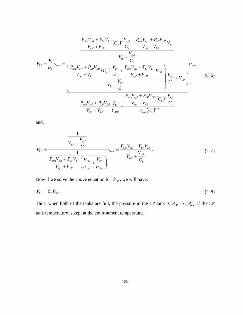
139
( )
( )
( )
( )
,
1
4
4atm
ratm
r
cylr
LPcyl
LPLPcylatm
atm
LP
LPcyl
LPLPcylatm
LPr
cyl
r
cyllp
LPLPcyl
LPLPcylatm
r
cylr
LPcyl
LPLPcylatm
r
cyllp
LPLPcyl
LPLPcylatm
r
cylr
LPcyl
LPLPcylatm
atmLP
CCV
CVV
VPVP
VVV
VPVP
VCV
CV
V
VVV
VPVPCV
CVV
VPVPCV
V
VVV
VPVPCV
CVV
VPVP
PP υ
υυ
υυ
γ
γ
γ
γ
−
+
+
++
+
⎟⎟⎠
⎞⎜⎜⎝
⎛+
⎟⎟⎟⎟⎟
⎠
⎞
⎜⎜⎜⎜⎜
⎝
⎛
+
+
++
+
+
+
+
++
+
+
==
(C.6)
and,
.1
1
r
cylLP
LPLPcylatmatm
atm
cyl
atm
LP
LPcyl
LPLPcylatm
r
cylLP
LP
CV
V
VPVP
VVVV
VPVP
CV
VP
+
+=
⎟⎟⎠
⎞⎜⎜⎝
⎛+
+
+
+= υ
υυ
(C.7)
Now if we solve the above equation for LPP , we will have:
.atmrLP PCP = (C.8)
Thus, when both of the tanks are full, the pressure in the LP tank is atmrLP PCP = if the LP
tank temperature is kept at the environment temperature.
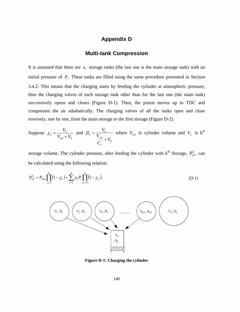
140
Appendix D
Multi-tank Compression
It is assumed that there are sn storage tanks (the last one is the main storage tank) with an
initial pressure of iP . These tanks are filled using the same procedure presented in Section
3.4.2. This means that the charging starts by feeding the cylinder at atmospheric pressure,
then the charging valves of each storage tank other than for the last one (the main tank)
successively opens and closes (Figure D-1). Then, the piston moves up to TDC and
compresses the air adiabatically. The charging valves of all the tanks open and close
reversely, one by one, from the main storage to the first storage (Figure D-2).
Suppose kcyl
kk VV
V+
=χ and k
r
cyl
kk
VCV
V
+=β where cylV is cylinder volume and kV is kth
storage volume. The cylinder pressure, after feeding the cylinder with kth Storage, kcylP , can
be calculated using the following relation:
( ) ( )∑ ∏∏= +==
−+−=k
i
k
ijjii
k
iiatm
kcyl PPP
1 11
.11 χχχ (D.1)
Figure D-1: Charging the cylinder
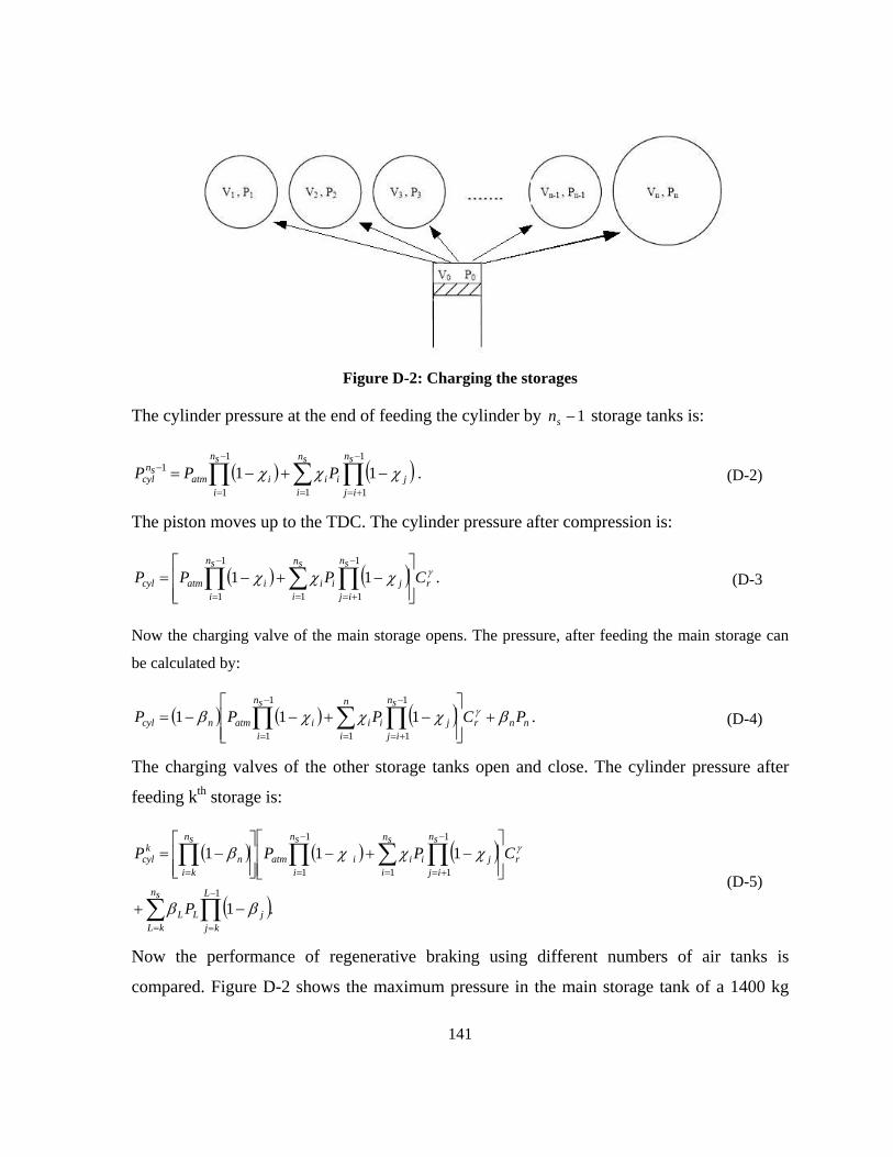
141
Figure D-2: Charging the storages
The cylinder pressure at the end of feeding the cylinder by 1−sn storage tanks is:
( ) ( ) .111
1
1
1
1
1 ∑ ∏∏=
−
+=
−
=
− −+−=sn
i
sn
ijjii
sn
iiatm
sncyl PPP χχχ
(D-2)
The piston moves up to the TDC. The cylinder pressure after compression is:
( ) ( ) .111
1
1
1
1
γχχχ r
sn
i
sn
ijjii
sn
iiatmcyl CPPP
⎥⎥⎦
⎤
⎢⎢⎣
⎡−+−= ∑ ∏∏
=
−
+=
−
=
(D-3
Now the charging valve of the main storage opens. The pressure, after feeding the main storage can
be calculated by:
( ) ( ) ( ) .1111
1
1
1
1nnr
n
i
sn
ijjii
sn
iiatmncyl PCPPP βχχχβ γ +
⎥⎥⎦
⎤
⎢⎢⎣
⎡−+−−= ∑ ∏∏
=
−
+=
−
=
(D-4)
The charging valves of the other storage tanks open and close. The cylinder pressure after
feeding kth storage is:
( ) ( ) ( )
( ).1
1 11
1
1
1
1
1
1
∏∑
∑ ∏∏∏−
==
=
−
+=
−
==
−+
⎥⎥⎦
⎤
⎢⎢⎣
⎡−+−
⎥⎥⎦
⎤
⎢⎢⎣
⎡−=
L
kjj
sn
kLLL
r
sn
i
sn
ijjii
sn
iiatm
sn
kin
kcyl
P
CPPP
ββ
χχχβ γ
(D-5)
Now the performance of regenerative braking using different numbers of air tanks is
compared. Figure D-2 shows the maximum pressure in the main storage tank of a 1400 kg
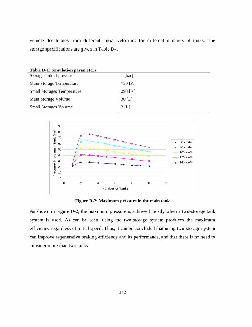
142
vehicle decelerates from different initial velocities for different numbers of tanks. The
storage specifications are given in Table D-1.
Table D-1: Simulation parameters Storages initial pressure 1 [bar]
Main Storage Temperature 750 [K]
Small Storages Temperature 298 [K]
Main Storage Volume 30 [L]
Small Storages Volume 2 [L]
Figure D-2: Maximum pressure in the main tank
As shown in Figure D-2, the maximum pressure is achieved mostly when a two-storage tank
system is used. As can be seen, using the two-storage system produces the maximum
efficiency regardless of initial speed. Thus, it can be concluded that using two-storage system
can improve regenerative braking efficiency and its performance, and that there is no need to
consider more than two tanks.
0
10
20
30
40
50
60
70
80
90
0 2 4 6 8 10 12
Number of Tanks
Pre
ssur
e in
the
mai
n Ta
nk (b
ar)
60 km/hr80 km/hr100 km/hr120 km/hr140 km/hr
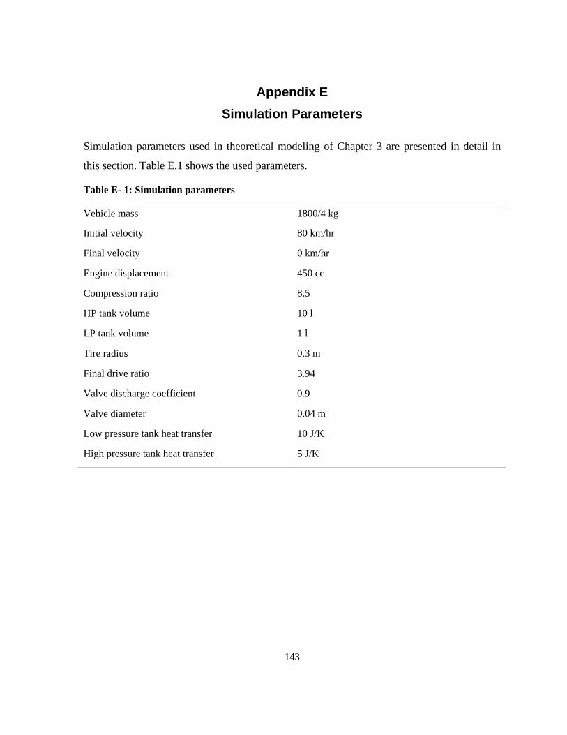
143
Appendix E
Simulation Parameters
Simulation parameters used in theoretical modeling of Chapter 3 are presented in detail in
this section. Table E.1 shows the used parameters.
Table E- 1: Simulation parameters
Vehicle mass 1800/4 kg
Initial velocity 80 km/hr
Final velocity 0 km/hr
Engine displacement 450 cc
Compression ratio 8.5
HP tank volume 10 l
LP tank volume 1 l
Tire radius 0.3 m
Final drive ratio 3.94
Valve discharge coefficient 0.9
Valve diameter 0.04 m
Low pressure tank heat transfer 10 J/K
High pressure tank heat transfer 5 J/K
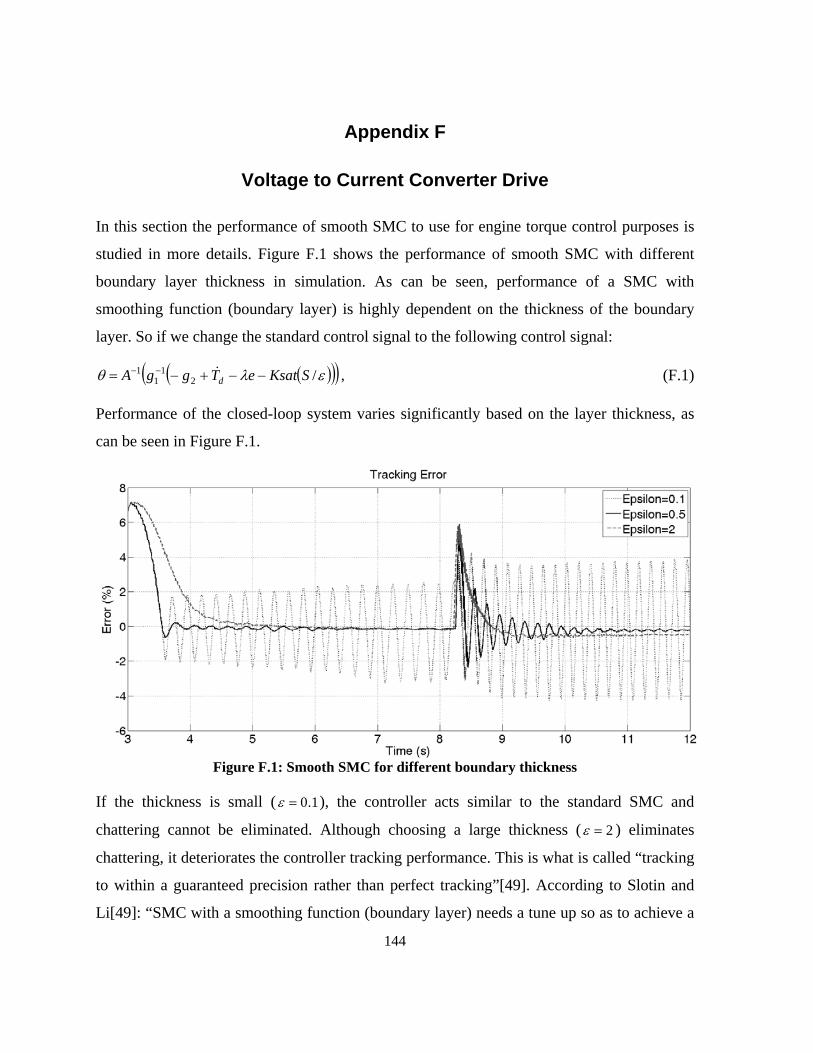
144
Appendix F
Voltage to Current Converter Drive
In this section the performance of smooth SMC to use for engine torque control purposes is
studied in more details. Figure F.1 shows the performance of smooth SMC with different
boundary layer thickness in simulation. As can be seen, performance of a SMC with
smoothing function (boundary layer) is highly dependent on the thickness of the boundary
layer. So if we change the standard control signal to the following control signal:
( )( )( ) ,/21
11 ελθ SKsateTggA d −−+−= −− & (F.1)
Performance of the closed-loop system varies significantly based on the layer thickness, as
can be seen in Figure F.1.
Figure F.1: Smooth SMC for different boundary thickness
If the thickness is small ( 1.0=ε ), the controller acts similar to the standard SMC and
chattering cannot be eliminated. Although choosing a large thickness ( 2=ε ) eliminates
chattering, it deteriorates the controller tracking performance. This is what is called “tracking
to within a guaranteed precision rather than perfect tracking”[49]. According to Slotin and
Li[49]: “SMC with a smoothing function (boundary layer) needs a tune up so as to achieve a
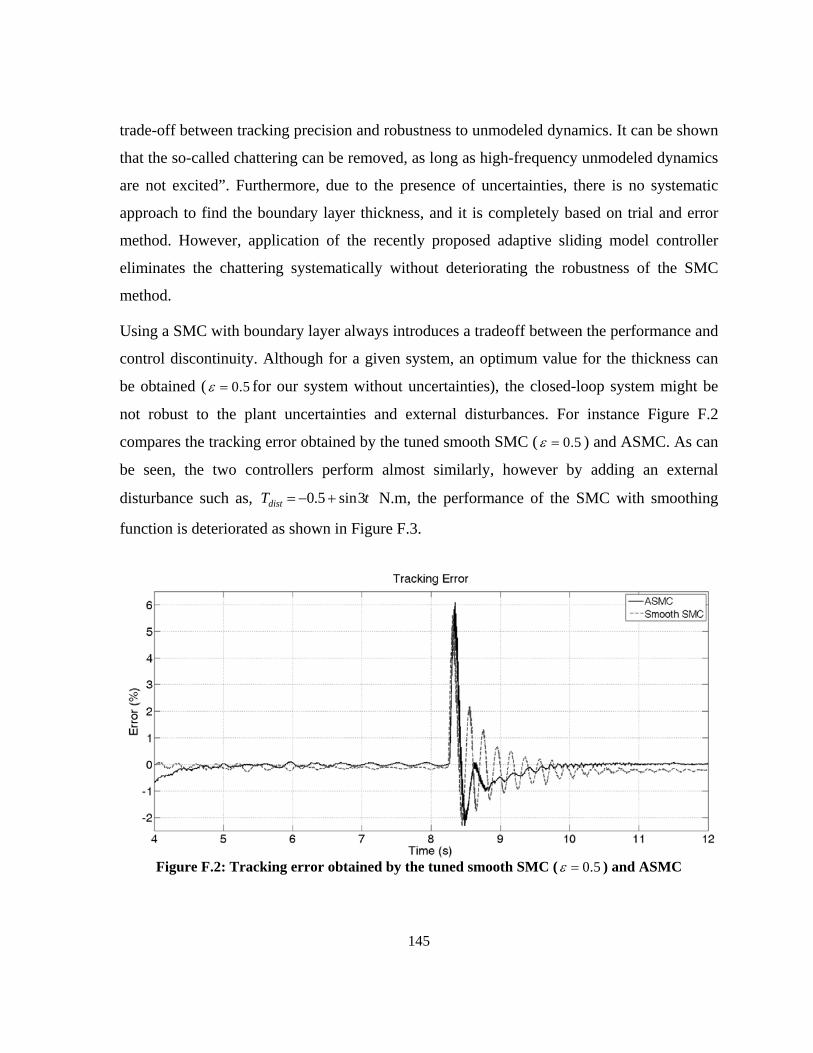
145
trade-off between tracking precision and robustness to unmodeled dynamics. It can be shown
that the so-called chattering can be removed, as long as high-frequency unmodeled dynamics
are not excited”. Furthermore, due to the presence of uncertainties, there is no systematic
approach to find the boundary layer thickness, and it is completely based on trial and error
method. However, application of the recently proposed adaptive sliding model controller
eliminates the chattering systematically without deteriorating the robustness of the SMC
method.
Using a SMC with boundary layer always introduces a tradeoff between the performance and
control discontinuity. Although for a given system, an optimum value for the thickness can
be obtained ( 5.0=ε for our system without uncertainties), the closed-loop system might be
not robust to the plant uncertainties and external disturbances. For instance Figure F.2
compares the tracking error obtained by the tuned smooth SMC ( 5.0=ε ) and ASMC. As can
be seen, the two controllers perform almost similarly, however by adding an external
disturbance such as, tTdist 3sin5.0 +−= N.m, the performance of the SMC with smoothing
function is deteriorated as shown in Figure F.3.
Figure F.2: Tracking error obtained by the tuned smooth SMC ( 5.0=ε ) and ASMC
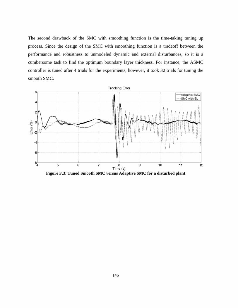
146
The second drawback of the SMC with smoothing function is the time-taking tuning up
process. Since the design of the SMC with smoothing function is a tradeoff between the
performance and robustness to unmodeled dynamic and external disturbances, so it is a
cumbersome task to find the optimum boundary layer thickness. For instance, the ASMC
controller is tuned after 4 trials for the experiments, however, it took 30 trials for tuning the
smooth SMC.
Figure F.3: Tuned Smooth SMC versus Adaptive SMC for a disturbed plant
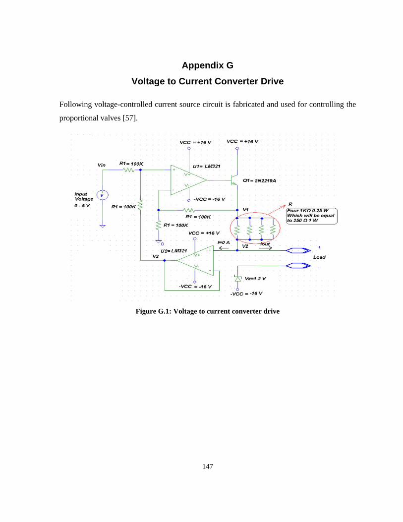
147
Appendix G Voltage to Current Converter Drive
Following voltage-controlled current source circuit is fabricated and used for controlling the
proportional valves [57].
Figure G.1: Voltage to current converter drive
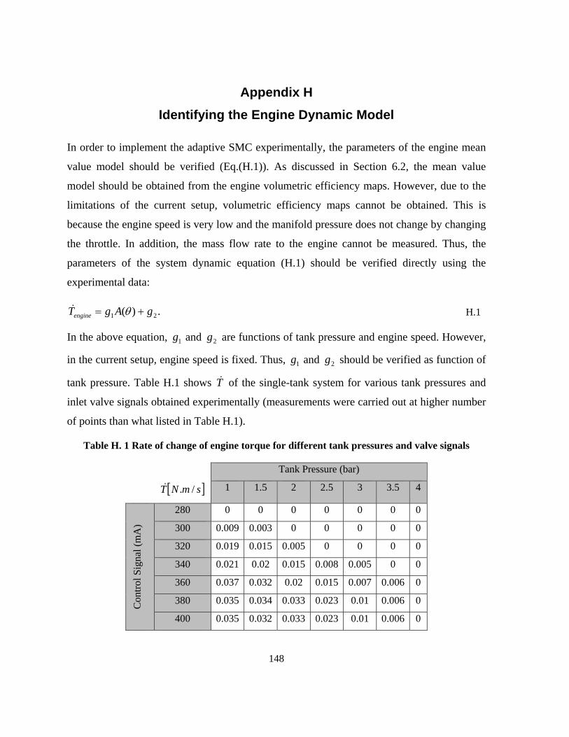
148
Appendix H Identifying the Engine Dynamic Model
In order to implement the adaptive SMC experimentally, the parameters of the engine mean
value model should be verified (Eq.(H.1)). As discussed in Section 6.2, the mean value
model should be obtained from the engine volumetric efficiency maps. However, due to the
limitations of the current setup, volumetric efficiency maps cannot be obtained. This is
because the engine speed is very low and the manifold pressure does not change by changing
the throttle. In addition, the mass flow rate to the engine cannot be measured. Thus, the
parameters of the system dynamic equation (H.1) should be verified directly using the
experimental data:
.)( 21 gAgTengine += θ& H.1
In the above equation, 1g and 2g are functions of tank pressure and engine speed. However,
in the current setup, engine speed is fixed. Thus, 1g and 2g should be verified as function of
tank pressure. Table H.1 shows T& of the single-tank system for various tank pressures and
inlet valve signals obtained experimentally (measurements were carried out at higher number
of points than what listed in Table H.1).
Table H. 1 Rate of change of engine torque for different tank pressures and valve signals
Tank Pressure (bar)
[ ]smNT /.& 1 1.5 2 2.5 3 3.5 4
Con
trol S
igna
l (m
A)
280 0 0 0 0 0 0 0
300 0.009 0.003 0 0 0 0 0
320 0.019 0.015 0.005 0 0 0 0
340 0.021 0.02 0.015 0.008 0.005 0 0
360 0.037 0.032 0.02 0.015 0.007 0.006 0
380 0.035 0.034 0.033 0.023 0.01 0.006 0
400 0.035 0.032 0.033 0.023 0.01 0.006 0
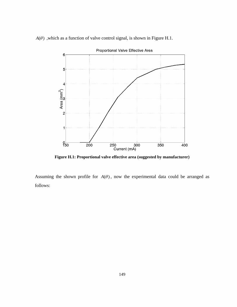
149
)(θA ,which as a function of valve control signal, is shown in Figure H.1.
Figure H.1: Proportional valve effective area (suggested by manufacturer)
Assuming the shown profile for )(θA , now the experimental data could be arranged as
follows:
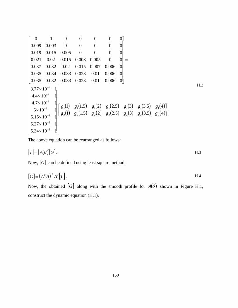
150
( ) ( ) ( ) ( ) ( ) ( ) ( )( ) ( ) ( ) ( ) ( ) ( ) ( ) .
45.335.225.1145.335.225.11
11034.511027.511015.511051107.41104.411077.3
0006.001.0023.0033.0032.0035.00006.001.0023.0033.0034.0035.00006.0007.0015.002.0032.0037.000005.0008.0015.002.0021.00000005.0015.0019.000000003.0009.00000000
2222222
1111111
6
6
6
6
6
6
6
⎥⎦
⎤⎢⎣
⎡
⎥⎥⎥⎥⎥⎥⎥⎥⎥
⎦
⎤
⎢⎢⎢⎢⎢⎢⎢⎢⎢
⎣
⎡
×××
××××
=
⎥⎥⎥⎥⎥⎥⎥⎥⎥
⎦
⎤
⎢⎢⎢⎢⎢⎢⎢⎢⎢
⎣
⎡
−
−
−
−
−
−
−
gggggggggggggg
H.2
The above equation can be rearranged as follows:
[ ] ( )[ ][ ] .GAT θ=& H.3
Now, [ ]G can be defined using least square method:
[ ] ( ) [ ] .1 TAAAG TT &−= H.4
Now, the obtained [ ]G along with the smooth profile for ( )θA shown in Figure H.1,
construct the dynamic equation (H.1).
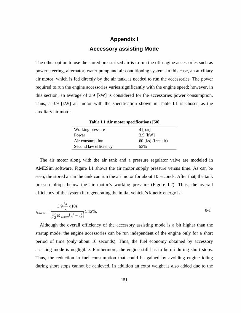
151
Appendix I Accessory assisting Mode
The other option to use the stored pressurized air is to run the off-engine accessories such as
power steering, alternator, water pump and air conditioning system. In this case, an auxiliary
air motor, which is fed directly by the air tank, is needed to run the accessories. The power
required to run the engine accessories varies significantly with the engine speed; however, in
this section, an average of 3.9 [kW] is considered for the accessories power consumption.
Thus, a 3.9 [kW] air motor with the specification shown in Table I.1 is chosen as the
auxiliary air motor.
Table I.1 Air motor specifications [58]
Working pressure 4 [bar] Power 3.9 [kW] Air consumption 60 [l/s] (free air) Second law efficiency 53%
The air motor along with the air tank and a pressure regulator valve are modeled in
AMESim software. Figure I.1 shows the air motor supply pressure versus time. As can be
seen, the stored air in the tank can run the air motor for about 10 seconds. After that, the tank
pressure drops below the air motor’s working pressure (Figure I.2). Thus, the overall
efficiency of the system in regenerating the initial vehicle’s kinetic energy is:
( ) %.122
1
109.3
22
21
overall ≅−
×=
vvM
ss
kJ
vehicle
η 8-1
Although the overall efficiency of the accessory assisting mode is a bit higher than the
startup mode, the engine accessories can be run independent of the engine only for a short
period of time (only about 10 seconds). Thus, the fuel economy obtained by accessory
assisting mode is negligible. Furthermore, the engine still has to be on during short stops.
Thus, the reduction in fuel consumption that could be gained by avoiding engine idling
during short stops cannot be achieved. In addition an extra weight is also added due to the
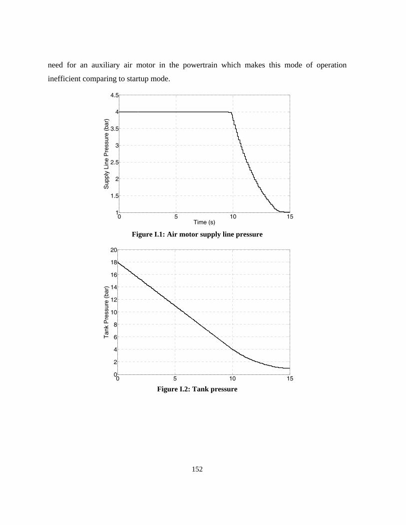
152
need for an auxiliary air motor in the powertrain which makes this mode of operation
inefficient comparing to startup mode.
Figure I.1: Air motor supply line pressure
Figure I.2: Tank pressure
0 5 10 151
1.5
2
2.5
3
3.5
4
4.5
Time (s)
Sup
ply
Line
Pre
ssur
e (b
ar)
0 5 10 150
2
4
6
8
10
12
14
16
18
20
Tan
k P
ress
ure
(bar
)
153
Reference
[1] "Transportation Statistics Annual Report," The Bureau of Transportation Statistics, 2008.
[2] Kluger, J., Harris, M., "Fuel Economy Benefits of Electric and Hydraulic Off Engine
Accessories," in SAE World Congress, 2007.
[3] Ali, I., Yang, K., Kim, S., "E3 System - A Two speed Accessory Belt Drive System for Reduced
Fuel Consumption," in SAE International Powertrains, Fuels and Lubricants Congress, 2008.
[4] Donitz, C., Vasile, L.,Onder, C., Guzzella, L., "Realizing a Concept for High Efficiency and
Excellent Drivability: The Downsized and Supercharged Hybrid Pneumatic Engine," in SAE
World Congress, 2009.
[5] Wang, Y., Megli, T., Haghgooie, M., "Modeling and control of electromechanical valve
actuator," in SAE World Congress, 2002.
[6] Giglio V., Lorio B. and Police G., "Analysis of advantages and of problems of electromechanical
valve actuators," in SAE World Congress, 2002.
[7] Pournazeri, M., Fazeli, A., Khajepour, A., "A cam-based electro-hydraulic variable valve timing
system for pneumatic hybrid engines," in ASME International Mechanical Engineering
Congress and Exposition IMECE09, 2009.
[8] Tai, C., Tsao, T., "Control of an electromechanical camless valve actuator," in Proceeding of the
American Control Conference, 2002.
[9] Amiri, M.,Esfahanian, M.,Hariri-Yazdi, M.,Esfahanian, V. , "Minimization of Power Losses in
Hybrid Electric Vehicles in View of the Prolonging of Battery Life," Journal of Power Sources,
vol. 10, no. 2, pp. 372-379, May 2009.
[10] I. Kim, "The Novel State of Charge Estimation Method for Lithium Battery Using Sliding Mode
Observer," Journal of Power Sources, vol. 163, pp. 584-590, 2006.
[11] Guzzella, L., Sciarretta, A., Vehicle Propulsion Systems Introduction to Modeling and
Optimization, 2nd ed. New York: Springer, 2007.
[12] Schechter, M., "New Cycle for Automobile Engines," in SAE World Congress, Detroit, 1999.
[13] Schechter, M., "Regenerative Compression Braking- A Low Cost Alternative to Electric
Hybrids," in SAE World Congress, 2000.
154
[14] Schechter M., "Operating a vehicle with braking energy recovery," 7231998, 2007.
[15] Tai, C.,Tsao, T., Levin, M. B. ,Barta, G., Schechter, M., "Using Camless Valvetrain for Air
Hybrid Optimization," in SAE World Congress, 2003.
[16] Kang, H.,Tai, C. ,Smith, E. ,Wang, X. ,Tsao, T. ,Stewart, J.,Blumberg, P.N. , "Demonstration of
Air-Power-Assist Engine Technology for Clean Combustion and Direct Energy Recovery in
Heavy Duty Application," in SAE Technical Paper # 2008-01-1197, 2008.
[17] Wang, X., "Modeling and Experiment of Compressed Air," University of California, Los
Angeles, A dissertation submitted in partial satisfaction of the requirements for the degree
Doctor of Philosophy in Mechanical Engineering 2008.
[18] Andersson, M., Johansson, B., Hultqvist, A., "An Air Hybrid for High Power Absorption and
Discharge," in SAE World Congress, 2005.
[19] Trajkovic, S.,Tunestal, P., Johansson, B., "Introductory Study of Variable Valve Actuation for
Pneumatic Hybridization," in SAE World Congress, 2007.
[20] Trajkovic, S.,Tunestal, P., Johansson, B., "Investigation of Different Valve Geometries and
Valve Timing Strategies and their Effect on Regenerative Efficiency for a Pneumatic Hybrid
with Variable Valve Actuation," in SAEWorld Congress, 2008.
[21] Trajkovic, S.,Tunestal, P., Johansson, B. , "Vehicle Driving Cycle Simulation of a Pneumatic
Hybrid Bus Based on Experimental Engine Measurements," in SAE World Congress, 2010.
[22] Ivanco, A.,Charlet, A.,Chamaillard, Y. ,Higelin, P. , "Energy Management Strategies for Hybrid-
Pneumatic Engine Studied on an," in SAE world congress, 2009.
[23] Donitz, C., Vasile, I., Onder, C., Guzzella, L., "Modelling and optimizing two- and four-stroke
hybrid pneumatic engines," Journal of Automobile Engineering, vol. 223, no. 2, 2009.
[24] Onitz, C. , Vasile, I. , Onder, C., Guzzella, L., "Dynamic Programming for Hybrid Pneumatic
Vehicles," in American Control Conference, Hyatt Regency Riverfront, St. Louis, MO, USA,
2009.
[25] Huang, K. D., Tzeng, S. C., "A new parallel-type hybrid electricvehicle," Applied Energy, no.
79, pp. 51-64, 2004.
[26] Huang, K. D., Tzeng, S. C., Chang, W. C., "Energy saving hybrid vehicle using a pneumatic
power system," Jorunal of Applied Energy, vol. 1, pp. 1-18.
155
[27] Huang, K. D.,Tzeng, S. C.,Ma, W. P., Chang, W. C. , "Hybrid pneumatic power system which
recycles exhaust-gas of an internal combustion engine," Applied Energy, vol. 82, pp. 117-132,
2005.
[28] Ehsani, M., Gao, Y., Gat, S., Emadi, A., Modern Electric Hybrid Electric, and Fuel Cell
Vehicles. Washington, D.C., USA: CRC Press, 2005.
[29] Cengel, Y., Boles, M., Thermodynamic: An Engineering Approach, 6th ed.: McGraw-Hill
Science, 2006.
[30] Ehrlich, GM., Gitzendanner, R., Puglia, F., Marsh, C., Bragg, B. J., "A Lithium Ion Cell for the
EMU Battery," in SAE Aerospace Power Systems Conference and Exposition, 1999.
[31] Joseph, P., Fellner, R., Miller, M., Shanmugasundaram, V., "Rechargeable Lithium-Ion Based
Batteries and Thermal Management for Airborne High Energy Electric Lasers," in SAE Power
Systems Conference, 2006.
[32] Ferguson, C. R., Internal Combustion Engines.: John Wiley & Sons, 1986.
[33] Heywood, J. B., Internal Combustion Engines Fundamentals, McGraw-Hill Science, Ed., 1988.
[34] Oliver, G., "Computer Simulation of Air Injection to Inlet Manifold On Turbocharged Engines,"
in FISITA 2006, 2006.
[35] Lee, C., Zhao, H. , Ma, T. , "Analysis of a Cost Effective Air Hybrid Concept," in SAE World
congress, 2009.
[36] Lee, C., Zhao, H., Ma, T., "The Perfromance Characteritics of a Production Oriented Air Hybrod
Powertrain," in SAE World Congress, 2010.
[37] Psanis, C., "Modelling and experomentation on air hybrid engine concept for automotive
application," Brunel University, A thesis submitted for the degree of Doctor of Philosophy 2007.
[38] Hosaka, T., Hamazaki, M., "Development of the variable valve timing and lift (Vtec) engine for
the Honda Nsx," in SAE Technical Paper 910008, 1991.
[39] Gafvert M., Arzen K., Pedersen L. and Bernhardsson B., "Control of GDI engines using torque
feedback exemplified by simulations," Journal of Control Engineering Practice, vol. 12, 2004.
[40] Carvalho, L., "Exergitic Analysis of Compressed Air for Vehicular Propulsion," in SAE World
Congress, 2008.
[41] Wagner, J., Dawson, D., Zeyu, L., "Nonlinear Air-to_Fuel Ratio and Engine Speed Control for
156
Hybrid Vehicles," IEEE Transactions on Vehicular Technology, vol. 52, no. 1, 2003.
[42] Souder, J., Hedrick, J. K., "Adaptive Sliding Mode Control of Air-Fuel Ratio in Internal
Combustion Engines," International Journal of Robust and Nonlinear, vol.
(DOI:10.1002/rnc.901)., pp. 525-541, 2004.
[43] Tang, H., Weng, L., Dong, Z., Yan, R., "Adaptive and Learning Control for SI Engine Model
with Uncertainties," IEEE/ASME Transactions on Mechatronics, vol. 14, no. 1, 2009.
[44] Slotine, J. J. E., Li, W., Applied Nonlinear Control.: Prentice-Hall Inc., 1991.
[45] Hendricks, E., "Engine Modeliing for Control Applications: A Critical Survey," Mechanica, vol.
32, pp. pp. 387-396, 1997.
[46] Hendricks, E., Sorenson, S.C., "Mean Value Modelling of Spark Ignition Engines," in SAE
International Congress and Exposition, vol. and Exposition Detroit, Michigan, 1999., Detroit,
Michigan, 1999.
[47] De Nicolao, G., Scattolini, R., Siviero, C., "Modelling the volumetric efficiency of IC engines:
Parametric, non-parametric and neural techniques," vol. 4, pp. 1405-1415, 1996.
[48] Zeinali, M., Notash, L., "Adaptive Sliding Mode Control with Uncertainty Estimator for Robot
Manipulators," Journal of Mechanism and Machine Theory, vol. 45, 2010.
[49] Slotine, J. and Li, W., Applied Nonlinear Control. New Jersey: Prentice hall, 1991.
[50] Chunji, L., "Global Asymptotic Stability of Generalized Lienard Equation," Trends in
Mathematics Information Center for Mathematical Sciences, vol. 4, no. 2, pp. 127-131,
December 2001.
[51] Kokotovic, P., Marino, R., "On vanishing stability regions in nonlinear systems with high-gain
feedback," IEEE Transactions on Automatic Control, vol. 31, no. 10, pp. 967-970, October 1986.
[52] Sundström, O.,Ambühl, D., Guzzella, L., "On Implementation of Dynamic Programming for
Optimal Control Problems with Final State Constraints," Oil & Gas Science and Technology,
vol. 65, no. 1, pp. 91-102, 2010.
[53] P´erez, L., Bossio, G., Moitre, D., Garc´ıa, G. , "Optimization of power management in an
hybrid electric vehicle using dynamic programming," Mathematics and Computers in
Simulation, vol. 73, pp. 244–254, 2006 2006.
[54] Brahma, A.,Guezennec, Y.,Rizzoni, G. , "Optiml Energy Managment in Series Hybrid Electric

157
Vehicles," in American Control Conference, Chicago, 2000.
[55] Ueno, K. ,Bye, R. E. , Hunter, K. S., "Compressor Efficiency Definitions," University of
Colorado, 2003.
[56] Chlumský, V., Reciprocating and rotary compressors. Prague: SNTL, 1965.
[57] Hosseini, M. www.astinco.com. [Online]. http://www.astinco.com/pdf/vccs.pdf
[58] TDI Tech development. [Online]. http://www.tdi-turbotwin.com/t30m.php