development of an ultrasonic sensing technique to measure
TRANSCRIPT
Development of an Ultrasonic Sensing
Technique to Measure Lubricant Viscosity
in Engine Journal Bearing In-Situ
PhD Thesis
Candidate: MICHELE M. SCHIRRU
Department: Mechanical Engineering
The Leonardo Centre for Tribology
Thesis submitted for the Degree of Doctor of Philosophy
January 2016
Supervisors: Prof. R. Dwyer-Joyce and Dr. M. Marshall
1
Table of Contents Summary .............................................................................................................................. 5
Chapter 1 Introduction ................................................................................ 8
Introduction .......................................................................................................................... 8
1.1Statement of the Problem................................................................................................... 8
1.2Project Aims ................................................................................................................... 11
1.3Thesis Layout ................................................................................................................. 11
Chapter 2 Background on Viscosity and Lubrication................................ 13
2.1Definition of Viscosity .................................................................................................... 13
2.1.1Viscosity Relation with Temperature ............................................................................. 14
2.1.2Viscosity Index ............................................................................................................ 14
2.1.3Viscosity and Pressure .................................................................................................. 15
2.1.4 Viscosity and Shear Rate ............................................................................................. 16
2.2 Viscosity Measurement .................................................................................................. 18
2.2.1 Capillary Viscometers ................................................................................................. 19
2.2.2 Rotational Viscometers ................................................................................................ 19
2.2.3 Falling Body Viscometers ............................................................................................ 21
2.2.4 Vibrational Viscometers .............................................................................................. 22
2.2.5 High Pressure Viscometers .......................................................................................... 23
2.2.6 High Shear Viscometers............................................................................................... 25
2.3 Engine Lubricating Oil Composition ............................................................................... 26
2.3.1 Base Oils .................................................................................................................... 27
2.3.2 Viscosity Modifiers ..................................................................................................... 28
2.3.2 Detergents .................................................................................................................. 29
2.4 Oil Classification by Viscosity ........................................................................................ 30
2.5 Lubrication Principles in Mechanical Components ............................................................ 31
2.5.1 The Stribeck Curve...................................................................................................... 31
2.5.2 Journal Bearing Lubrication ......................................................................................... 32
2.6 Conclusions ................................................................................................................... 32
Chapter 3 Background on Ultrasound ....................................................... 39
3.1 Introduction to Ultrasound .............................................................................................. 39
3.2 Ultrasound and Material Properties ................................................................................. 40
3.3 Ultrasonic Transducers ................................................................................................... 42
3.3.1 The Piezoelectric Effect ............................................................................................... 42
3.3.2 Ultrasonic Transducer Type ......................................................................................... 43
2
3.4 Characteristics of Ultrasonic Signals ............................................................................... 47
3.5 Transducers Arrangements ............................................................................................. 48
3.6 Reflection of Ultrasound Waves at Interface. ................................................................... 49
3.6.1 Reflection and Transmission in a Three-Layered System ............................................... 53
3.6.2 Reflection of Shear Waves at Solid-Liquid Boundary .................................................... 54
Chapter 4 Literature review ...................................................................... 59
4.1 The Crystal Resonator .................................................................................................... 59
4.2 The Resonating Plate/Rod............................................................................................... 60
4.3 Reflectance Methodologies ............................................................................................. 61
4.3.1 The Newtonian reflection model................................................................................... 62
4.3.2 The Greenwood Model ................................................................................................ 64
4.4 The Attenuation Method ................................................................................................. 65
4.5 Ultrasonic Spectroscopy Methods ................................................................................... 66
4.6 Ultrasonic Resonator to Analyse Lubricating Oils ............................................................ 67
4.7 Comparison of Ultrasonic Viscometers and Conventional Viscometers.............................. 70
4.8 Conclusions ................................................................................................................... 71
Chapter 5 A Novel Ultrasonic Model for Non-Newtonian Fluids .............. 74
5.1 Introduction ................................................................................................................... 74
5.3 The Ultrasonic Model for Non-Newtonian Fluids ............................................................. 75
5.4 Comparison of Models ................................................................................................... 77
5.5 Non-Newtonian Ultrasonic Model Sensitivity Analysis .................................................... 80
5.6 Conclusions ................................................................................................................... 82
Chapter 6 Viscosity Measurement at an Aluminium-Oil Boundary .......... 83
6.1 Ultrasonic Apparatus ...................................................................................................... 83
6.1.1 The Transducers .......................................................................................................... 84
6.1.2 The Cables .................................................................................................................. 84
6.1.3 Thermocouple Calibration............................................................................................ 85
6.1.4 Test Lubricants ........................................................................................................... 86
6.1.5 Experimental Protocol ................................................................................................. 86
6.2 Signal Processing ........................................................................................................... 87
6.4 Conventional Reflectance Technique: Acoustic Mismatch ................................................ 91
6.5 Conclusions ................................................................................................................... 93
Chapter 7 The Matching Layer Method .................................................... 93
7.1 Origins of the Matching Layer Methodology.................................................................... 93
7.2 Matching Layer Theory .................................................................................................. 94
3
7.3 Measurement Apparatus ................................................................................................. 98
7.3.1 Instrumentation ........................................................................................................... 98
7.3.2 Test Cell and Matching Layer ...................................................................................... 98
7.3.3 Samples Tested ........................................................................................................... 99
7.4 Signal Processing and Data Analysis ............................................................................... 99
7.5 Results .........................................................................................................................101
7.5.1 Measurement Sensitivity Increment .............................................................................101
7.5.2 Viscosity Results for Newtonian Oils...........................................................................103
7.5.3 The Empirical Correlation Between Viscosity and Reflection Coefficient ......................104
7.5.3 Viscosity Results for Fully Formulated Engine Oils ......................................................105
7.6 Effect of Polymer Concentration and Excitation Frequency..............................................108
7.7 Effect of Temperature on Ultrasonic Matching Layer Viscometry ....................................111
7.7.1 Samples Tested ..........................................................................................................111
7.7.2 Experimental Protocol ................................................................................................111
7.7.3 Results.......................................................................................................................111
7.8 Effect of Pressure on Ultrasonic Matching Layer Viscometry...........................................114
7.8.1 Materials....................................................................................................................114
7.8.2 Signal Processing .......................................................................................................116
7.8.3 Experimental Protocol ................................................................................................116
7.8.4 Results.......................................................................................................................117
7.9 Conclusions ..................................................................................................................120
Chapter 8 Viscosity Measurement in a Journal Bearing ......................... 122
8.1 Apparatus .....................................................................................................................122
8.1.1 The Journal Bearing Test Rig ......................................................................................123
8.1.2 Ultrasonic Viscometer Probe .......................................................................................124
8.1.3 The Slip Ring .............................................................................................................125
8.1.4 Triggering and Data Acquisition..................................................................................126
8.1.5 Reflection Coefficient Acquisition in Journal Bearings .................................................127
8.2 Experimental Protocol ...................................................................................................128
8.3 Results .........................................................................................................................129
8.3.1 Effect of Seizure.........................................................................................................133
8.4 Analytical Simulation of Journal Bearing Viscosity Field ................................................135
8.4.1 Power Losses .............................................................................................................142
8.5 Preliminary Application to a Real Bearing ......................................................................145
8.6 Conclusions ..................................................................................................................146

4
Chapter 9 Conclusions ............................................................................. 147
9.1 The Ultrasonic Model for Non-Newtonian Fluids ............................................................147
9.2 The Quarter Wavelength Matching Layer Sensing Technique ..........................................147
9.3 Application of the Matching Layer Method in a Journal Bearing ......................................148
9.4 Future Directions ..........................................................................................................148

5
SUMMARY This work presents a novel technique to measure viscosity in-situ and in real time in engine
component interfaces by means of an ultrasonic technique. Viscosity is a key parameter in the
characterization of lubrication regime in engine parts because it can be related to friction in the
contact, and to the lubricant film thickness.
Ultrasound is a non-destructive and non-invasive technique that is based on the reflection of sound
from interfaces. The reflection from a solid-air boundary can identify, for instance, the presence of a
crack in a material, while reflection from a solid-liquid interface can help detecting the properties of
the liquid sample. Reflection of longitudinal waves measures fluid film thickness and chemical
composition, while the reflection of ultrasonic shear waves measures the fluid viscosity. The viscosity
measurements based on ultrasonic reflection from solid-fluid boundaries are referred to as reflectance
viscometry techniques. Common ultrasonic reflectance viscometry methods can only measure the
viscosity of Newtonian fluids. This work introduces a novel model to correlate the ultrasonic shear
reflection coefficient with the viscosity of non-Newtonian oils by means of the Maxwell model
analogy. This algorithm overcomes the limitation of previous models because it is suitable for the
analysis of common engine oils, and because it relies only on measurable parameters. However,
viscosity measurements are prohibitive at the metal-oil interfaces in auto engines because when the
materials in contact have very different acoustic impedances the sound energy is almost totally
reflected, and there is very little interaction between the ultrasonic wave and the lubricant. This
phenomenon is called acoustic mismatch. When acoustic mismatch occurs, any valuable information
about the liquid properties is buried in measurement noise. To prove this, the common reflectance set-
up was tested to measure the viscosity of different lubricants (varying from light base oils to greases)
using aluminium as solid boundary. More than 99.5% of the ultrasonic energy was reflected for the
different oils, and accurate viscosity measurement was not possible because the sensitivity of the
ultrasonic measurement at the current state of the art is of ±0.5%. Consequently, the discrimination by
viscosity of the oil tested was not possible.
In this study a new approach is developed. The sensitivity of the ultrasonic reflectance method is
enhanced with a quarter wavelength matching layer material. This material is interleaved between
metal and lubricant to increment the ultrasonic measurement sensitivity. This layer is chosen to have
thickness and mechanical properties that induce the ultrasonic wave to resonate at the solid-liquid
interface, at specific frequencies. In this work, resonance is associated with the destructive interaction
between the wave that is incident to the matching layer and the wave that is reflected at the matching
layer-oil interface. This solution brings a massive increment in the ultrasonic measurement sensitivity.
The matching layer technique was first tested by enhancing the sensitivity of the aluminium-oil set-up
that was affected by acoustical mismatch. A thin polyimide layer was used as a matching layer
between aluminium and the engine oil. This probe was used as ultrasonic viscometer to validate the
sensing technique by comparison with a conventional viscometer and by applying a temperature and
pressure variation to the samples analysed. The results showed that the ultrasonic viscometer is as
precise as a conventional viscometer when Newtonian oils are tested, while for Non-Newtonian oils
the measurement is frequency dependent. In particular, it was noticed that at high ultrasonic frequency
only the viscosity of the base of the oil was measured. The ultrasonic viscometer was used to validate
the mathematical model based on the Maxwell analogy for the correlation of the ultrasonic response
with the liquid viscosity.

6
At a second stage, this technique was implemented in a journal bearing. The ultrasonic viscometer
was mounted in the shaft to obtain the first viscosity measurement along the circumference of a
journal bearing at different rotational speeds and loads. The ultrasonic viscometer identified the
different viscosity regions that are present in the journal bearing: the inlet, the regions characterized
by the rise in temperature at the contact and the maximum loaded region were the minimum film
thickness occurs. The results were compared with the analytical isoviscous solution of the Reynolds
equation to confirm that the shape of the angular position-viscosity curves was correct.
Finally, the method was preliminarily tested on a coated shell bearing to show that the coating
presents in bearing, like iron-oxide or babbit, is a good matching layer for the newly developed
ultrasonic viscometer technique. This means that ultrasonic transducers, with sizes as small as a pencil
tip, have the potential to be mounted as viscometers in real steel bearings where the coating layer in
contact with the fluid acts as a matching layer. Overall, the results obtained showed that this technique
provides robust and precise viscosity measurements for in-situ applications in engine bearings.

7
Nomenclature
| | Reflection coefficient modulus (dimensionless)
Am Ultrasonic measurement amplitude (V)
Ar Ultrasonic reference Amplitude (V)
B Bearing width (m)
c Speed of sound (ms-1
)
c Bearing clearance (m)
E Young Modulus (Pa)
f Frequency (Hz)
FFT Fast Fourier Transform
G Shear modulus (Pa)
G’ Storage modulus (Pa)
G’’ Loss modulus (Pa)
G∞ Infinite shear modulus (Pa)
h Oil film thickness (m)
k Spring stiffness (Nm)
P Pressure (Pa)
R Complex reflection coefficient (dimensionless)
R Radius (m)
S Sommerfield Number (dimensionless)
T Temperature (°C)
T Transmission coefficient (dimensionless)
tm Matching layer thickness (m)
u Particle displacement (m)
W Load (N)
Ẇ Power losses (W)
z Material acoustic impedance (Rayl)
Liquid acoustic impedance (Rayl)
Solid acoustic impedance (Rayl) α Pressure-Viscosity coefficient (GPa
-1)
α Attenuation coefficient (Npm-1
)
δ Penetration depth (m)
η Dynamic viscosity (Pas)
σy Shear stress (Pa)
𝜀 Spring deformation (m)
𝜃 Reflection coefficient phase (radians)
𝜆 Wavelength (m)
μ Friction coefficient (dimensionless)
Material density (kgm-3
)
𝜏 Relaxation time (s)
𝜔 Angular frequency (rad/s)
𝜔 Rotational speed (s-1
)
Chapter 1 Introduction
8
Chapter 1 Introduction .
Introduction This chapter describes the reason and the aims of the project. The major role of viscosity in engine
lubrication is highlighted by showing the correlation of this parameter to wear mechanisms, and the
fuel economy market direction. Ultrasound is presented as the ideal non-invasive technology to build
a novel tool to measure viscosity in-situ and real time in operating engines. The advantages of this
tool are presented and described. Finally, the thesis layout reports a brief description of each thesis
chapter.
1.1 Statement of the Problem
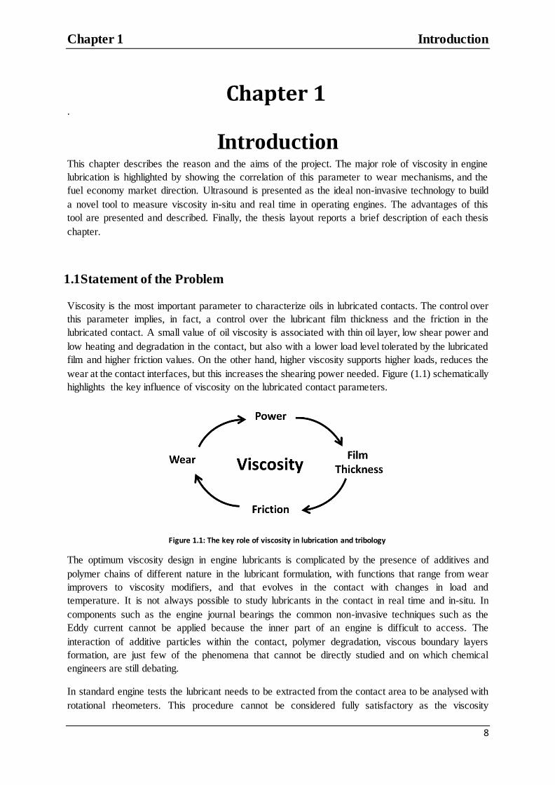
Viscosity is the most important parameter to characterize oils in lubricated contacts. The control over
this parameter implies, in fact, a control over the lubricant film thickness and the friction in the
lubricated contact. A small value of oil viscosity is associated with thin oil layer, low shear power and
low heating and degradation in the contact, but also with a lower load level tolerated by the lubricated
film and higher friction values. On the other hand, higher viscosity supports higher loads, reduces the
wear at the contact interfaces, but this increases the shearing power needed. Figure (1.1) schematically
highlights the key influence of viscosity on the lubricated contact parameters.
Figure 1.1: The key role of viscosity in lubrication and tribology
The optimum viscosity design in engine lubricants is complicated by the presence of additives and
polymer chains of different nature in the lubricant formulation, with functions that range from wear
improvers to viscosity modifiers, and that evolves in the contact with changes in load and
temperature. It is not always possible to study lubricants in the contact in real time and in-situ. In
components such as the engine journal bearings the common non-invasive techniques such as the
Eddy current cannot be applied because the inner part of an engine is difficult to access. The
interaction of additive particles within the contact, polymer degradation, viscous boundary layers
formation, are just few of the phenomena that cannot be directly studied and on which chemical
engineers are still debating.
In standard engine tests the lubricant needs to be extracted from the contact area to be analysed with
rotational rheometers. This procedure cannot be considered fully satisfactory as the viscosity
Chapter 1 Introduction
9
measured in a bulk is different from the one expected in thin layers and at the high shear rates and
pressures in operating engine conditions. Although test rigs can be used to simulate operating engine
shear rate conditions, for example the ultra-high shear viscometer (UHSV), the measurements from
such instrumentations cannot recreate the temperature, pressure and wear that occur in the real
lubricated contacts.
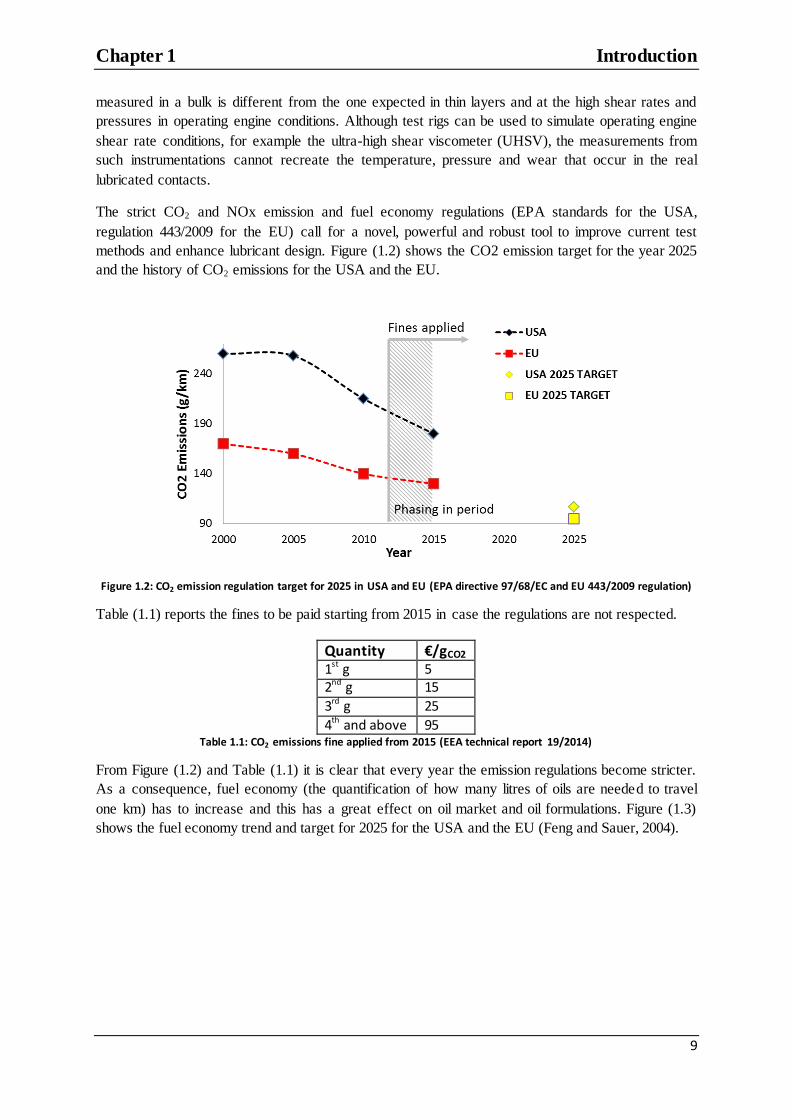
The strict CO2 and NOx emission and fuel economy regulations (EPA standards for the USA,
regulation 443/2009 for the EU) call for a novel, powerful and robust tool to improve current test
methods and enhance lubricant design. Figure (1.2) shows the CO2 emission target for the year 2025
and the history of CO2 emissions for the USA and the EU.
Figure 1.2: CO2 emission regulation target for 2025 in USA and EU (EPA directive 97/68/EC and EU 443/2009 regulation)
Table (1.1) reports the fines to be paid starting from 2015 in case the regulations are not respected.
Quantity €/gCO2 1st g 5 2nd g 15
3rd g 25
4th and above 95 Table 1.1: CO2 emissions fine applied from 2015 (EEA technical report 19/2014)
From Figure (1.2) and Table (1.1) it is clear that every year the emission regulations become stricter.
As a consequence, fuel economy (the quantification of how many litres of oils are needed to travel
one km) has to increase and this has a great effect on oil market and oil formulations. Figure (1.3)
shows the fuel economy trend and target for 2025 for the USA and the EU (Feng and Sauer, 2004).

Chapter 1 Introduction
10
Figure 1.3: Fuel economy target for 2025 in USA and EU (Feng and Sauer. 2004)
Figure (1.3) shows that the lubricant oil market has to point towards thinner oils. This is because
lower viscosity oils bring to less friction and consequently to less energy losses in the engine and to
higher fuel economy. However, when the viscosity is too low there is risk of wear due to solid-solid
contact in engine parts. Therefore, an optimum viscosity has to be achieved to balance performance
and regulations requirements. Figure 1.4 shows the trend in oil manufacturing between 2002 and 2008
for passenger cars in the EU (source The Lubrizol Corp. © survey).
Figure 1.4: Oil grade change between 2002 and 2008 in passenger vehicles market in the EU (source The Lubrizol corp.© survey)
At the same time, the oil formulation has to respect the emission regulation and this leads to
formulations with lower SAPS (sulphated ash, phosphorous, sulphur). To guarantee low viscosity, but
high engine durability and low SAPS, the oil industry is developing new polymeric oil additives that
act as viscosity modifier, wear improvers and anti-oxidant, just to cite a few.
In spite of the improvements in oil manufacturing, respecting the emission and fuel economy target
remains one of the biggest industrial challenges. An example of this is given when Volkswagen
suffered a US$18 billion fine for not respecting EPA‟s USA pollutions emission standards in

Chapter 1 Introduction
11
September 2015, roughly $30,000 / fault vehicle, equivalent to ¼ of the trade mark value as reported
by (Vlasic and Kessler, 2015). The formation and emission of harmful particles is controlled by
contact friction, oil temperature and pressure and is then correlated with the oil viscosity.
In this scenario, it appears clear that a novel technique to design and measure lubricant property is
needed. Ultrasound was chosen to develop this tool because it is the most versatile non-invasive
technology. The ultrasonic set-up can be miniaturized to fit the complex engine geometry and receive
data from contact areas otherwise inaccessible such as journal bearing contact interfaces. This
technique allows direct correlation of the energy of the reflected sound wave at a solid-liquid
boundary with the viscosity. Though viscosity measurement by means of ultrasonic technique has
been possible since the 1950s (Mason, 1948), application of this technique in many practical
applications such us in engine has not been possible due to the acoustic mismatch between steel and
lubricant. In this work, this limitation has been overcome by interleaving a matching layer between
the metal and the oil. It has been found that in a real component the matching layer can be constituted
by the coating, and this allows the application of this technique in real engines, opening up the
possibility of the first in-situ viscosity measurements.
1.2 Project Aims
The aim of this work was to develop a novel viscometer that can be used in real time and in-situ to
improve the current engine test techniques, to help designing more effective lubricants and to better
understand oil evolution in the contact.
The objectives of the project were:
Development of a mathematical model to correlate the ultrasound reflection to viscosity. This
model has to overcome the limitation of the current Newtonian methodologies to be applied
in the analysis of Non-Newtonian lubricants.
Validate the model by comparison with previously developed Newtonian models.
Development of an experimental method to successfully measure viscosity at a metal-oil
interface by means of ultrasound technology.
Compare the results acquired from the ultrasound viscometer with the results from a
conventional viscometer.
Mount the ultrasound viscometer into a journal bearing test rig to obtain the circumferential
viscosity profile.
1.3 Thesis Layout
This work is divided into nine chapters. This section reports a brief summary for all the chapters.
Chapter 2: Background on viscosity and lubrication. This chapter gives a fundamental knowledge
of what viscosity is and how it is measured. Attention is given in particular to the relationship
between viscosity and temperature, pressure and shear rate. The chapter covers also the basic aspects
of engine lubricants formulation and classification. Finally, in chapter 2.5, the basic concepts of
journal bearing lubrication are presented.

Chapter 1 Introduction
12
Chapter 3: Background on ultrasound. This chapter provides the reader with the basic knowledge
of ultrasound. The chapter starts with the basic ultrasound definition and relation of sound with the
material properties. It follows an accurate description of the different set-up and transducers used for
ultrasound measurements. Finally the reflection and transmission of ultrasound waves at boundaries is
studied in detail for normal and angular incidence and for two and three-layered systems.
Chapter 4: Literature review. This chapter describes the different ultrasonic methodologies
developed so far to measure viscosity. This chapter aims to show the application found by shear
waves in industry for viscosity measurement and the limits of the current state of the art. Particular
attention is given to the reflectance method that has been chosen in this research to undertake
viscosity measurement.
Chapter 5: A novel ultrasonic model for Non-Newtonian oils . This chapter describes in depth the
novel analytical model developed to calculate viscosity using the ultrasound method. The Maxwell
viscosity is correlated to the ultrasonic reflection coefficient and the analytical results are compared to
the expected results from common Newtonian based models.
Chapter 6: Viscosity measurements at an aluminium-oil boundary. This chapter describes the
instrumentation employed for the ultrasound acquisition and reports the results from the first
experiments in this work. Ultrasound reflection coefficient is acquired at an aluminium-oil boundary,
for different samples, and this parameter is converted to viscosity using different analytical models.
The high error in the results show that such a measurement is not practically possible by employing
the common ultrasonic reflectance technique.
Chapter 7: The matching layer method. This chapter describes the approach used to overcome the
limitations of the common reflectance technique. A matching layer is interposed between the metal
and oil interface to allow a better response from the reflected wave at the solid-oil boundary. This
novel method to measure viscosity is explained in detail. The chapter starts with the theory at the
heart of the method. The methodology is then implemented to analyse the effect of frequency, shear
rate, temperature and pressure on the viscosity and the results are compared with the viscosity
measured with a common cone-on-plate viscometer.
Chapter 8: Viscosity measurement in journal bearing . In this chapter the matching layer
methodology is tested for in-situ and real time viscosity measurement in a journal bearing test rig. At
first the set-up and the experimental protocol are presented. Different lubricants are tested for
different loads and rotational speed of the shaft. Finally the circumferential viscosity results are
presented and then discussed.
Chapter 9: Conclusions . In this section the results and finding of the research are summarized. The
chapter highlights the usefulness of the research results and suggestions for future works are outlined.

Chapter 2 Background on Viscosity and Lubrication
13
Chapter 2 Background on Viscosity
and Lubrication
Background on Viscosity and Lubrication
This chapter introduces the basic concepts of viscosity and lubrication. The optimization of the
lubricant viscosity plays a crucial role in preventing wear mechanisms in engineering components.
The chapter starts with the basic definition of viscosity and the relation of viscosity with temperature,
load and shear rate. This is followed by an overview of the current conventional methods to measure
viscosity and on the composition of engine lubricant. Subsequently the different lubrication regimes
are described with particular attention to the analysis of different lubrication stages in a journal
bearing, the case study in this research.
2.1 Definition of Viscosity
Figure (2.1) schematically shows the contact of two solid components in relative motion separated by
a fluid layer. For this situation, the relation between force F applied to the “Component 2”, the
relative velocity gradient u and fluid film thickness h is:
(2.1)
Where A is the wet surface area and the proportionality constant is called viscosity.
Figure 2.1: Schematic representation of a lubricated contact with two components in relative motion
Shear viscosity therefore defines the resistance offered by a fluid to an applied shear stress.
Rearranging equation (2.1) it is possible to obtain the following definition for the viscosity:
⁄ (2.2)
and consequently:
(2.3)

Chapter 2 Background on Viscosity and Lubrication
14
where is the shear stress and is the shear rate. When expressed in Pas, the shear viscosity is
referred to as dynamic viscosity, measured in P (Poiseuille) where 1P=0.1Pas. The viscosity can be
also calculated as kinematic viscosity when the dynamic viscosity is divided by the density of the oil:
(2.4)
where ν is the kinematic viscosity. The kinematic viscosity is measured in St (Stokes). Kinematic
viscosity is used to quantify the resistance to the fluid flow. Fluid viscosity is sensitive to
thermodynamic and stress changes in the lubricated system and especially to temperature, pressure
and shear rate variations.
2.1.1 Viscosity Relation with Temperature
The lubricant viscosity decreases with an increment in temperature because the particles dispersed in
the fluid will increase their oscillatory speed and atomic bonds become weaker thus offering an
overall less resistance to motion. The relation between viscosity and temperature is described by
several empirical laws, the most precise of which being the Vogel equation (Crouch and Cameron,
1961):
(2.5)
In this equation a, b and c are constants defined by knowing three values of viscosity at three known
temperatures and T is the temperature at which the viscosity is measured.
2.1.2 Viscosity Index
The viscosity index describes how oil viscosity changes with the temperature. This is an empirical
parameter that was introduced by Dean and Davis (1929) and is measured as:
(2.6)
Where L is the viscosity at 40°C of an oil of 0 VI having the same viscosity at 100°C of the oil whose
VI has to be calculated, H is the viscosity at 40°C of an oil of 100 VI having the same viscosity at
100°C as the oil whose VI has to be calculated, U is the viscosity at 40°C of the oil whose VI has to be
calculated. The values of L and H are tabled in the ASTM standard D2270 (1998). The viscosity index
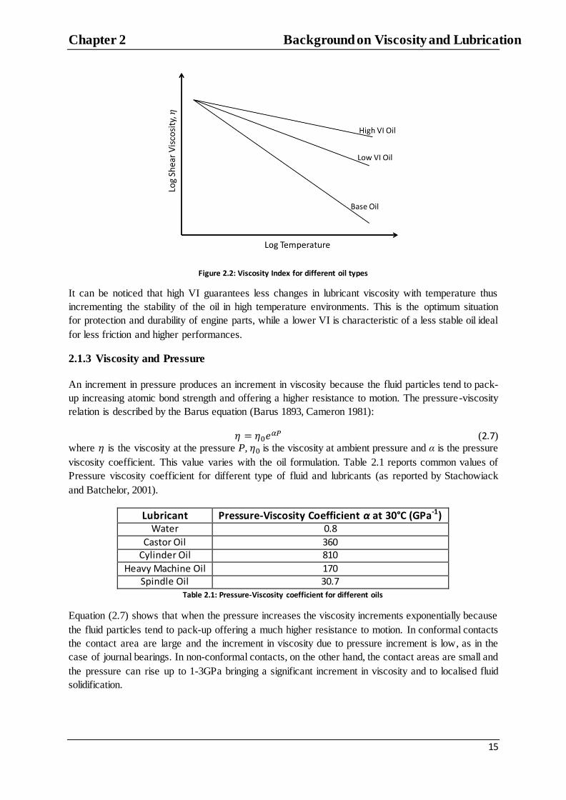
is one of the most important in the classification of lubricants. Figure (2.2) compares the viscosity
index for base oils and polymer oils with high and low VI.
Chapter 2 Background on Viscosity and Lubrication
15
Figure 2.2: Viscosity Index for different oil types
It can be noticed that high VI guarantees less changes in lubricant viscosity with temperature thus
incrementing the stability of the oil in high temperature environments. This is the optimum situation
for protection and durability of engine parts, while a lower VI is characteristic of a less stable oil ideal
for less friction and higher performances.
2.1.3 Viscosity and Pressure
An increment in pressure produces an increment in viscosity because the fluid particles tend to pack-
up increasing atomic bond strength and offering a higher resistance to motion. The pressure-viscosity
relation is described by the Barus equation (Barus 1893, Cameron 1981):
(2.7)
where is the viscosity at the pressure P, is the viscosity at ambient pressure and α is the pressure
viscosity coefficient. This value varies with the oil formulation. Table 2.1 reports common values of
Pressure viscosity coefficient for different type of fluid and lubricants (as reported by Stachowiack
and Batchelor, 2001).
Lubricant Pressure-Viscosity Coefficient α at 30°C (GPa-1) Water 0.8
Castor Oil 360 Cylinder Oil 810
Heavy Machine Oil 170 Spindle Oil 30.7
Table 2.1: Pressure-Viscosity coefficient for different oils
Equation (2.7) shows that when the pressure increases the viscosity increments exponentially because
the fluid particles tend to pack-up offering a much higher resistance to motion. In conformal contacts
the contact area are large and the increment in viscosity due to pressure increment is low, as in the
case of journal bearings. In non-conformal contacts, on the other hand, the contact areas are small and
the pressure can rise up to 1-3GPa bringing a significant increment in viscosity and to localised fluid
solidification.

Chapter 2 Background on Viscosity and Lubrication
16
2.1.4 Viscosity and Shear Rate
In perfectly Newtonian fluids the shear stress is proportional to the shear rate through the
proportionality constant shear viscosity, as shown in equation (2.3). This means that for purely
Newtonian oils viscosity is not dependent on shear rate. In practice perfectly Newtonian fluids do not
exist at the very high shear rates encountered in engine machinery, and oils with high additive
concentrations or complex molecular structure show Non-Newtonian behaviour. For these lubricants
the relation between stress and viscosity is non-linear. The relation of Non-Newtonian oils viscosity
with shear rate is quite complex and various mechanisms are involved. The main categories of Non-
Newtonian fluids are the pseudoplastic, or shear thinning, and dilatant, or shear thickening. For the
first category, the viscosity decreases as the shear rate increases because the random positioned
molecules tend to align thus offering less resistance to the shear, as shown in Figure (2.3 a). On the
other hand, shear thickening oils have suspensions of polymer particles with high solid content. When
there is no shear applied the solid particle will have a closed-up formation. When shear is applied the
voids between the solid particles expand in way that not enough liquid can fill them. This results in an
increment to the resistance to shear applied as shown in Figure (2.3 b). Another category of shear
dependent fluid is constituted by the Bingham fluid. These fluids “mimic” solid behaviour at low
shear and start flowing only after a sufficient stress is applied. The minimum stress at which Bingham
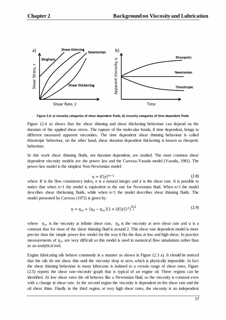
fluids flow is called the yield stress. Figure (2.4 a) shows the different shear rate-shear stress curves
for the different strain-dependent fluid type described in this chapter.
Figure 2.3: a) Shear thinning oil, b) Shear thickening oil
Chapter 2 Background on Viscosity and Lubrication
17
Figure 2.4: a) viscosity categories of shear dependent fluids, b) viscosity categories of time dependent fluids
Figure (2.4 a) shows that the shear thinning and shear thickening behaviour can depend on the
duration of the applied shear stress. The rupture of the molecular bonds, if time dependent, brings to
different measured apparent viscosities. The time dependent shear thinning behaviour is called
thixotropic behaviour, on the other hand, shear duration dependent thickening is known as rheopetic
behaviour.
In this work shear thinning fluids, not duration dependent, are studied. The most common shear
dependent viscosity models are the power law and the Carreau-Yasuda model (Yasuda, 1981). The
power-law model is the simplest Non-Newtonian model:
| | (2.8) where K is the flow consistency index, n is a natural integer and is the shear rate. It is possible to
notice that when n=1 the model is equivalent to the one for Newtonian fluid. When n>1 the model
describes shear thickening fluids, while when n<1 the model describes shear thinning fluids. The
model presented by Carreau (1972) is given by:
| |
(2.9)
where is the viscosity at infinite shear rate, is the viscosity at zero shear rate and a is a
constant that for most of the shear thinning fluid is around 2. This shear rate dependent model is more
precise than the simple power-law model for the way it fits the data at low and high shear. In practice
measurements of are very difficult so this model is used in numerical flow simulations rather than
as an analytical tool.
Engine lubricating oils behave commonly in a manner as shown in Figure (2.3 a). It should be noticed
that the oils do not shear thin until the viscosity drop to zero, which is physically impossible. In fact
the shear thinning behaviour in many lubricants is isolated to a certain range of shear rates. Figure
(2.5) reports the shear rate-viscosity graph that is typical of an engine oil. Three regions can be
identified. At low shear rates the oil behaves like a Newtonian fluid, so the viscosity is constant even
with a change in shear rate. In the second region the viscosity is dependent on the shear rate and the
oil shear thins. Finally in the third region, at very high shear rates, the viscosity is an independent
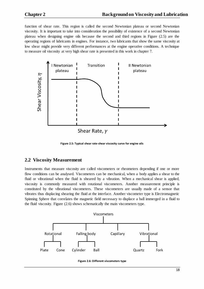
Chapter 2 Background on Viscosity and Lubrication
18
function of shear rate. This region is called the second Newtonian plateau or second Newtonian
viscosity. It is important to take into consideration the possibility of existence of a second Newtonian
plateau when designing engine oils because the second and third regions in Figure (2.5) are the
operating regions of lubricants in engines. For instance, two lubricants that show the same viscosity at
low shear might provide very different performances at the engine operative conditions. A technique
to measure oil viscosity at very high shear rate is presented in this work in chapter 7.
Figure 2.5: Typical shear rate-shear viscosity curve for engine oils
2.2 Viscosity Measurement
Instruments that measure viscosity are called viscometers or rheometers depending if one or more
flow conditions can be analysed. Viscometers can be mechanical, when a body applies a shear to the
fluid or vibrational when the fluid is sheared by a vibration. When a mechanical shear is applied,
viscosity is commonly measured with rotational viscometers. Another measurement principle is
constituted by the vibrational viscometers. These viscometers are usually made of a sensor that
vibrates thus displacing shearing the fluid at the interface. Another viscometer type is Electromagnetic
Spinning Sphere that correlates the magnetic field necessary to displace a ball immerged in a fluid to
the fluid viscosity. Figure (2.6) shows schematically the main viscometers type.
Figure 2.6: Different viscometers type

Chapter 2 Background on Viscosity and Lubrication
19
A wide number of viscometers exist and it would be impossible, and out of the purpose of this
research, to enumerate and describe them all in this chapter. In this section the main mechanical shear
type viscometers are analysed to give the reader the perspective of some of the options the market
offers to measure viscosity with conventional systems (sections 2.2.1-2.2.3). Along with this, the main
commercial type of vibrational viscometers (section 2.2.4) are described. In this research a vibrational
viscometer is developed and the results are compared with the reading from a conventional
mechanical shear rheometer. Finally, high pressure and high shear viscometry is described in relation
to tribological and automotive applicability.
2.2.1 Capillary Viscometers
Capillary viscometers measure viscosity by correlating the time a fluid samples takes to travel through
a capillary with the kinematic viscosity of the sample. The higher the fluid viscosity, the longer the
time needed by the sample to travel through the capillary. Figure (2.7) shows the scheme of capillary
viscometers.
Figure 2.7: Schematic representation of a capillary viscometer
Kinematic viscosity in capillary viscometers is measured as (Webster, 1999):
(
)
(2.10)
where is the difference in pressure at the inlet and outlet of the viscometer, D is the diameter of
the capillary, Q is the fluid volume flow rate and L is the length of the capillary.
2.2.2 Rotational Viscometers
Rotational viscometers are used to measure dynamic viscosity. In this type of viscometer the fluid is
placed between two surfaces, one stationary, while the second one rotates. The viscosity measurement
is either done by measuring the change in rotational speed given a fixed torque or by measuring the
torque change given a constant rotational speed. The main rotational viscometers are cylinder or cone-
on-plate. Figure (2.8) reports the typical setup for a rotating cylinder viscometer. Here the gap

Chapter 2 Background on Viscosity and Lubrication
20
between two concentric cylinders is filled with the fluid sample. The inner cylinder rotates thus
shearing the contact interface between solid and liquid.
Figure 2.8: Schematic representation of a cylinder rotational viscometer
The viscosity is measured as follows (Webster, 1999):
(
)
𝜔
(2.11)
where is a parameter dependent on the cylinder geometry, 𝜔 is the rotational speed, T is the applied
torque and L is the effective length of the cylinder at which the torque is measured. Figure (2.9)
reports the setup for a cone-to-plate viscometer. The operating principle is the same as in the rotating
cylinder, but in this case the rotating part is cone shaped. This type of viscometer is the most used on
the market as just a small drop of fluid is needed and very thin films can be analysed.
Figure 2.9: Schematic representation of a cone-on-plate viscometer

Chapter 2 Background on Viscosity and Lubrication
21
In cone type viscometers the viscosity is measured as:
𝜃
𝜔 (2.12)
where 𝜃 is the cone angle of incidence and R is the plate radius. The shear rate generated in
rotational viscometer varies from in conventional viscometers to in
recently developed ultra-high shear viscometers (UHSV). The same measurement principle is adopted
in other viscometers such as the plate-to-plate viscometer.
2.2.3 Falling Body Viscometers
Falling body viscometers measure viscosity by correlating the time a body takes to travel through a
capillary with the resistance offered by the fluid and so to the viscosity. Figure (2.10) reports two
examples of falling body viscometers.
Figure 2.10: a) Falling sphere viscometer, b) falling cylinder viscometer
Figure (2.8a) shows schematically a falling ball viscometer, Figure (2.8b) shows a falling cylinder
viscometers. In this section only the case of the falling body is analysed, but similar consideration can
be made to obtain the value of viscosity from the falling cylinder viscometer type. The restraining
force F resulting from the viscous drag in a fluid for a spherical body is calculated from the Stokes
law as:
(2.13)
where is the radius of the sphere and is the terminal velocity of the falling body. By balancing
equation (2.13) with the buoyancy force exerted on a ball then viscosity can be calculated as:
(2.14)
More accurate equations can be obtained by taking into consideration the wall effect and the finite
length of the capillary.

Chapter 2 Background on Viscosity and Lubrication
22
2.2.4 Vibrational Viscometers
Different types of vibrational viscometers exist. The rotational and the turning-fork viscometer
measure the viscosity by determining the amount of power necessary to displace the fluid of a certain
quantity. The quartz resonators measure the change in resonant driving frequency when an oscillating
quartz crystal is submerged in a liquid. The sonic and ultrasonic viscometer measures the reflection of
sound at a solid-liquid interface and correlate the amount of reflected energy to the viscosity of the
fluid samples. In this section the rotational and the turning fork viscometer are described, while the
quartz resonator is briefly described in section 4.1. The ultrasound viscometer is described in depth in
chapter 3, 4 and 5 and the applications of this novel technique are described in sections 6 to 8.
Figure (2.11) shows schematically a turning fork viscometer.
Figure 2.11: Schematic representation of a vibrational fork viscometer
The rotational viscometer operates similarly, but in that case only a cantilever beam is present. The
measuring system is driven by electromagnetic power and the natural frequency of the system is
determined by the mass and spring constant of the measuring system. The energy consumed by the
measuring system will only be the viscous term of the liquid because the inertial force and the
restorative force of the spring balance each other. The motion equation of the system is:
(2.15)
where F is the excitation force, m is the mass of the system c is the viscosity-density coefficient, K is
the spring constant and x is the displacement of the system. After integration, equation (2.15) gives:
𝜔
(2.16)
where 𝜔 is the natural vibrational frequency of the system. The coefficient c is calculated by setting
x and 𝜔 as constant.

Chapter 2 Background on Viscosity and Lubrication
23
2.2.5 High Pressure Viscometers
The viscometers described in sections 2.2.1 to 2.2.4 can be modified to work as pressure viscometers
to study the pressure-viscosity characteristic of engine oils. Basically, the viscometer is enclosed in a
pressurized vessel where the oil to be study is brought to the desired pressure normally using pressure
intensifiers. Bair (2007) enumerated and described the characteristic of the most common high
pressure viscometers:
High pressure capillary viscometer. the first attempt of pressurizing the capillary
viscometers was made by Warburg and Sachs (1884), but the maximum performance (at the
current state of the art) were achieved by Novak and Winer (1968) who managed to obtain
viscosity at 0.6 GPa at the temperature of 150°C. Figure (2.12) shows the viscometer.
Figure 2.12: The Novak and Winer high pressure capillary viscometer. R1 and R2 are the translating pistons the displace the fluid and P1 is the piston that determine the pressure at which the fluid is measured (Bair, 2007)
The high pressure is obtained with two pressure intensifiers. The capillary of the viscometer is
placed in between the pressure intensifiers and the pressure is measured with strain gage
transducers.
High pressure dropping body viscometer. These are divided in falling ball and falling
cylinder viscometers. The high pressure falling ball viscometer consists of a falling ball
capillary inserted in a pressure vessel. The vessel pressurizes the tube externally and
internally. Figure (2.13) shows the high pressure ball viscometer by Sawamura et al. (1990).

Chapter 2 Background on Viscosity and Lubrication
24
Figure 2.13: Sawamura high pressure falling body viscometer (Bair, 2007)
In this set-up, the light from a lamp is refracted from the glass ball across a pair of sapphire
windows. This allows measurement of the falling time of the ball. This type of viscometer,
however, presents some limitations such as complex flow and a limited range of viscosity that
can be studied. The falling cylinder viscometer by Irving and Barlow (1971) provided
considerable improvement because the sinker does not have to travel along all the length of
the capillary. This is because the sinker position is detected monitoring the inductance of
different coils that are positioned around the viscometer. This allows using any desirable
length of the capillary for the measurement. Figure (2.14) shows the high pressure falling
cylinder viscometer. The operative principle is very similar to the falling body viscometer, but
for the falling cylinder the falling time is measured by detecting the making and breaking of
an electric contact once the sinker touches an electric pin at the bottom of the capillary.

Chapter 2 Background on Viscosity and Lubrication
25
Figure 2.14: Irving and Barlow high pressure falling body viscometer. The falling body (9) descends through the capillary
(1). The electrical coils (10) allows the identification of the position of the falling body (Bair, 2007)
2.2.6 High Shear Viscometers
Common viscometers can measure viscosity at shear rates up to 10,000 s-1
. The shear rate in engine
journal bearings can exceed 10,000,000 s-1
(Selby and Miller, 1995). Starting from the 60s, novel high
shear viscometers were designed to measure oil properties at the operating engine conditions and to
fulfil the requirements of the ASTM standards. The operative principle of the high shear viscometer
is the same as the rotating cylinder viscometer, but the gaps between the cylinder are very thin and the
rotational speed of the cylinder is much higher. The first high shear viscometer was the tapered
bearing shear viscometer, patented by the Savant Inc. (1979), and its design has been used for
decades. Figure (2.15) shows this viscometer schematically.
Figure 2.15: Tapered bearing high shear viscometer (Selby and Miller, 1995)
In this geometry, the stator and the rotor are separated by a gap of just a few micrometres. This means
that if the rotor spins at high rotational speed (usually ω>2000 rpm) then high shear rates are obtained.
This measurement from this viscometer is affected by the shear heating that occurs at the contact area.
This causes distortions in the film shape that affect the accuracy of the measurement at shear rates
higher than 3,000,000 s-1
. These limitations have been recently overcome by the USV ultra high shear
Chapter 2 Background on Viscosity and Lubrication
26
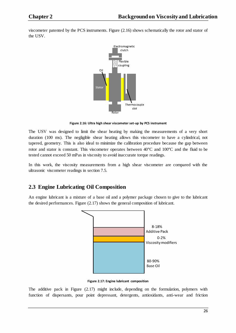
viscometer patented by the PCS instruments. Figure (2.16) shows schematically the rotor and stator of
the USV.
Figure 2.16: Ultra high shear viscometer set-up by PCS instrument
The USV was designed to limit the shear heating by making the measurements of a very short
duration (100 ms). The negligible shear heating allows this viscometer to have a cylindrical, not
tapered, geometry. This is also ideal to minimize the calibration procedure because the gap between
rotor and stator is constant. This viscometer operates between 40°C and 100°C and the fluid to be
tested cannot exceed 50 mPas in viscosity to avoid inaccurate torque readings.
In this work, the viscosity measurements from a high shear viscometer are compared with the
ultrasonic viscometer readings in section 7.5.
2.3 Engine Lubricating Oil Composition
An engine lubricant is a mixture of a base oil and a polymer package chosen to give to the lubricant
the desired performances. Figure (2.17) shows the general composition of lubricant.
Figure 2.17: Engine lubricant composition
The additive pack in Figure (2.17) might include, depending on the formulation, polymers with
function of dispersants, pour point depressant, detergents, antioxidants, anti-wear and friction

Chapter 2 Background on Viscosity and Lubrication
27
modifiers. A polymer is a long chain of repeating monomers arranged in different architectures, as
shown in Figure (2.18).
Figure 2.18: Some polymer architectures
Figures (2.17) and (2.18) show the complexity involved in the study and design of lubricants.
Depending on the polymers nature (geometry and chemical composition) and the number of species
present in a lubricant the analysis of contact in engine is complicated by the interaction of these
species and their evolution (or deterioration) in new compounds inside the contact. In the following
sections the base oil type and viscosity modifier and detergent additives are analysed (sections 2.3.1-
2.3.2) because the engine lubricant tested in this work are made manly of these polymers.
2.3.1 Base Oils
Base oils are long chain hydrocarbons refined from crude oil (mineral oils) or they can be
synthetically made. Tables (2.3) and (2.4) report respectively the composition of mineral oils and their
official API classification.
Element % by weight Carbon 83-87
Hydrogen 11-14 Sulphur 0-8
Nitrogen 0-1
Oxygen 0.5 Metals 0.02
Table 2.3: Mineral oil composition (Arora, 2005)
API Classification I II III % saturates <90 >90 >90
%Sulfur >0.03 <0.03 <0.03
VI 80-120 80-120 >120 Table 2.4: API base oil official classification (source API)

Chapter 2 Background on Viscosity and Lubrication
28
An “unofficial” classification exists also for synthetic base oils. This classification includes two other
groups: Group IV or the synthetic Polyalphaolephin (PAO) group and Group V or Ester group.
API Classification IV-PAO V- Ester % saturates - -
%Sulfur 0 0
VI 130 135 Table 2.5: Unofficial synthetic base oil classification (source API)
The 90% of base oil market is constituted of oils from the first three groups, while the synthetic oils
constitute only 1% of the overall sales due to the high costs involved in the manufacturing process.
2.3.2 Viscosity Modifiers
Viscosity modifiers are polymers that increase the viscosity of the base oil and are among the most
important additives. They are designed to increase the viscosity at low temperature as little as they
can, while thickening the base at high temperatures, as shown in Figure (2.19).
Figure 2.19: Viscosity-Temperature characteristic behaviour with the addition of viscosity modifier
It is possible to notice that the viscosity modifiers increase the VI. The aim of current light duty
commercial vehicle market is to increase oil‟s VI for higher economy and durability as engine
components wear is decreased. Another decisive factor in the viscosity modifier design is the polymer
shear stability. This is the ability of a fluid to maintain its viscosity after a stress is applied. When a
stress is applied to a polymer chain this might break or strain/compress with no rupture. For a
viscosity modifier polymer it is desired that the polymer does not break because otherwise the
viscosity modifier properties of the polymeric chain deteriorates over time. Table (2.6) reports a list
of the main polymers used as viscosity modifiers with benefits and negative effects on the engine
parts.

Chapter 2 Background on Viscosity and Lubrication
29
Polymer Advantages Disadvantages Olefin Copolymer
(OCP) Cost effective. High thickening. Good solubility.
Weak low temperature performances. Contribute to piston deposits in engines.
Maleic Styrene Copolymer (MSC)
Cost effective High thickening.
Weak low temperature performances. Leave high deposits.
Poly(alkyl methacrylates) (PMA)
Great low temperature properties. Thermal and oxidative stability. Excellent engine test performance. Used as VM and pour point depressant.
Expensive. Cannot be made as a solid. Relative low thickening.
Table 2.6: Main viscosity modifier polymers characteristics (Covitch and Trickett, 2015)
2.3.2 Detergents
Detergents are polymers used in engine oils, gear oils and automatic transmission lubricants. Their
major roles are to clean internal engine parts, neutralise acids of combustion and inhibit oxidation. All
these functions enhance durability of engine parts. Figure (2.20) shows schematically a detergent
polymer particle.
Figure 2.20: Schematic representation of detergent polymers in contact to an engine surface
Detergent particles come in different shapes, but Figure (2.20) gives a good idea of the general
detergent polymer structure and behaviour. This polymer is mainly made of a fatty oil soluble tail and
a charged polarised head. The detergent polymers head stick to the iron surface at the contact interface
with the lubricant oil. This allows inhibiting corrosion and removing undesired polarised particle from
the surface. Table (2.7) reports the most commonly used detergent polymer and highlights advantages
and disadvantages of using one polymer over the other.

Chapter 2 Background on Viscosity and Lubrication
30
Detergent type Advantages Disadvantages Sulfonates Excellent detergency.
Cost effective. No antioxidancy.
Phenates Good detergency. Antioxidant performance.
Expensive.
Salicylates
Excellent antioxidant. Good detergency. Sulphur free.
Expensive.
Table 2.7: Unofficial synthetic base oil classification (Mortier and Orszulik, 2010)
2.4 Oil Classification by Viscosity
Oil viscosity in combustion engines is classified by the SAE J-300 standard. This standard establishes
different oil grades and is updated every two years to meet the latest industrial standards. Table (2.8)
reports the oil grades viscosity as stated in the SAE J-300 standard of April 2013.
SAE Viscosity
Grade
Low-Temperature (°C) cranking
viscosity, mPas
Low-Temperature (°C) Pumping
Viscosity, mPas
Low-Shear rate
kinematic viscosity
( at 100 °C Min
Low-Shear rate
kinematic viscosity
( at 100 °C Max
High Shear rate
viscosity (mPas) at
150 °C Min
0W 6200 at -35°C 60000 at -40°C 3.8 5W 6600 at -30°C 60000 at -35°C 3.8
10W 7000 at -25°C 60000 at -30°C 4.1 15W 7000 at -20°C 60000 at -25°C 5.6
20W 9500 at -15°C 60000 at -20°C 5.6
25W 13000 at -10°C 60000 at -15°C 9.3 16 6.1 <8.2 2.3
20 6.9 <9.3 2.6 30 9.3 <12.5 2.9
40 12.5 <16.3 3.5 40 12.5 <16.3 3.7
50 16.3 <21.9 3.7
60 21.9 <26.1 3.7 Table 2.8: SAE J-300, oil classification by viscosity (source SAE standards)
In this table the letter W means “winter” and characterize the so called multigrade oils. This category
of lubricants have good cold start capabilities, but tend to shear thin at high shear rates that occur in
components such as journal bearing. The oils that appear in Table (2.8) without the letter W are called
monograde because they meet only one SAE grade. It has to be highlighted that in the SAE J-300 the
extreme grades are the ones more exposed to change. For example the grade SAE 16 has been
recently added to lower the limit of HSHT (high shear high temperature) applications. Also, the
upgrades are made to meet the pollution emission regulations; engines that operate with oils outside
the limits of this table are considered harmful and such engines need to be upgraded or dismissed.

Chapter 2 Background on Viscosity and Lubrication
31
2.5 Lubrication Principles in Mechanical Components
2.5.1 The Stribeck Curve
Separation of sliding surfaces by means of a lubricant layer is necessary to reduce friction and wear in
mechanical components assemblies. Two sliding components in contact operate in ideal condition
when this separation is achieved. In practice three different lubrication regimes occur among
mechanical components in contact: boundary lubrication, mixed lubrication and hydrodynamic (HD).
The Stribeck curve, Figure (2.21), identifies these regimes in a graph where the non-dimensional
product of viscosity η, rotational speed U and the load in the contact area W is plotted against the
friction μ.
Figure 2.21: The Stribeck curve
The first region of the graph is called boundary lubrication because the lubrication film is not formed
and contact between asperities occurs. In this region of the Stribeck curve the load is completely
carried by the solid asperities in contact because there is absence of the hydrodynamic lift. Because of
this, the boundary lubrication region is characterized by high values of friction coefficient. This is the
case for most of the start-up conditions of mechanical components.
Once the components are in relative motion the contact area between asperities reduces and a
lubricant film starts forming. This causes a drastic drop in friction that is characteristic of the mixed
lubrication region. In this lubrication region the lubricant film starts forming and the load is partially
supported by the solid asperities and by the forming lubricant film. Figure (2.22) shows schematically
a mixed lubrication regime situation.

Chapter 2 Background on Viscosity and Lubrication
32
Figure 2.22: Schematic representation of mixed lubrication contact
When mixed lubrication occurs, the hydrodynamic lift of the lubricating layer is still not sufficient to
form a full lubricated layer. Consequently, the contact region is characterized by pockets of oil and
asperities in contact. The mixed lubrication region physical nature is still a matter of debate. Spikes
(Spikes and Olver, 2003) states: “The key feature of mixed lubrication is considered to be that it
contains a mixture, i.e., the presence of two distinctly different regimes of lubrication within one
contact, one being conventional fluid-film lubrication … and the other something else. This begs the
question as to what is the 'something else”. That „something else‟ can be arise from complex solid-
solid asperities interaction, formation of micro-EHD (elasto-hydrodynamic) regions, and/or formation
of thin layer of lubricant that behaves differently compared to the bulk case.
As a full lubrication film is formed, the value of load per unit area decreases drastically and the
product of viscosity and rotational speed increases. Consequently the friction increases linearly
because of the increment in viscous drag forces. The region characterized by the absence of asperity
contact is referred to as hydrodynamic lubrication zone. HD lubrication was first studied by Tower
(1883) and Reynolds (1886) developed the governing equation describing fluid film separating two
wedge shaped components:
(
)
(2.17)
where h is the film thickness and U is the velocity gradient. This equation has been developed to suit
the analysis of different components geometries such as plain journal bearings.
2.5.2 Journal Bearing Lubrication
Journal bearings are widely used in automotive engines and their main purpose is to support and align
the load from a rotating shaft, for instance the crankshaft. Depending on the load direction the journal
bearing can be axial or radial. In this work the case of radial journal bearing is studied. In contrast to
ball or cylindrical roller bearings, the surface of the journal bearing is in direct contact with the shaft
to support. Figure (2.23) shows the main components constituting the journal bearing assembly. This
is made of a shaft or journal in direct contact with the bearing or bush. The separation of journal and
bush in automotive engines is usually obtained through a layer of liquid lubricant.
Chapter 2 Background on Viscosity and Lubrication
33
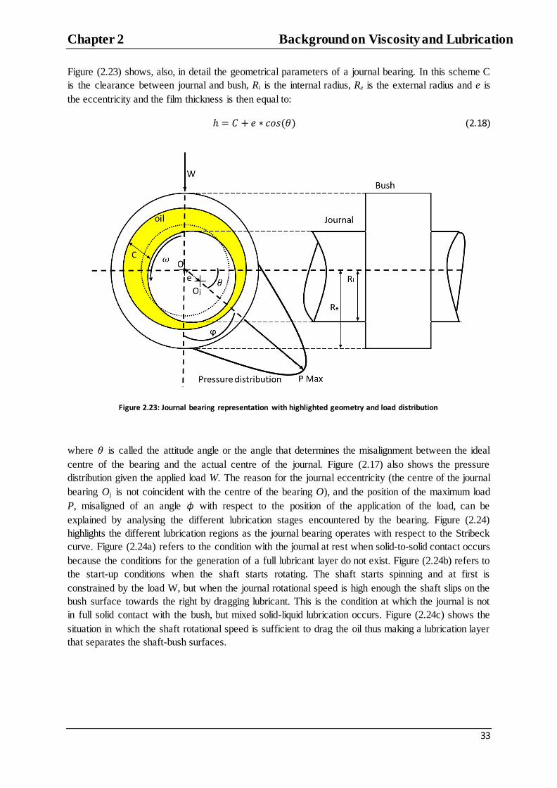
Figure (2.23) shows, also, in detail the geometrical parameters of a journal bearing. In this scheme C
is the clearance between journal and bush, Ri is the internal radius, Re is the external radius and e is
the eccentricity and the film thickness is then equal to:
𝜃 (2.18)
Figure 2.23: Journal bearing representation with highlighted geometry and load distribution
where 𝜃 is called the attitude angle or the angle that determines the misalignment between the ideal
centre of the bearing and the actual centre of the journal. Figure (2.17) also shows the pressure
distribution given the applied load W. The reason for the journal eccentricity (the centre of the journal
bearing Oj is not coincident with the centre of the bearing O), and the position of the maximum load
P, misaligned of an angle ϕ with respect to the position of the application of the load, can be
explained by analysing the different lubrication stages encountered by the bearing. Figure (2.24)
highlights the different lubrication regions as the journal bearing operates with respect to the Stribeck
curve. Figure (2.24a) refers to the condition with the journal at rest when solid-to-solid contact occurs
because the conditions for the generation of a full lubricant layer do not exist. Figure (2.24b) refers to
the start-up conditions when the shaft starts rotating. The shaft starts spinning and at first is
constrained by the load W, but when the journal rotational speed is high enough the shaft slips on the
bush surface towards the right by dragging lubricant. This is the condition at which the journal is not
in full solid contact with the bush, but mixed solid-liquid lubrication occurs. Figure (2.24c) shows the
situation in which the shaft rotational speed is sufficient to drag the oil thus making a lubrication layer
that separates the shaft-bush surfaces.

Chapter 2 Background on Viscosity and Lubrication
34
Figure 2.24: a) Journal bearing at rest solid-solid contact, b) rotation of shaft initiate the friction coefficient decreases and the lubrication is mixed, c) full hydrodynamic lubrication
The determination of the maximum eccentricity and the minimum film thickness is complex and
dependent on many parameters; the most important of which are the radius of the shaft, the width of
the bush, the rotational speed of the shaft, the surface finish, and the applied load. The design of
journal bearings starts with the Reynolds equation, equation (2.17). For a narrow bearing (L/D<1/3)
the Reynolds equation becomes (Cameron, 1966):
𝜀 𝜃
𝜀 𝜃 (
)
(2.19)
where y is the length on the axial direction. This solution is very convenient, but in practice L/D<1/3
are not common in engines because the bearing vibrations are not well-damped (Alford, 1911).
Common values of L/D ratio ranges normally between 0.6 to 1 for bearings used in engines. Because
of this the Reynolds equation was solved numerically by Raimondi and Boyd (1958) for bearings with
different L/D ratio. Figure (2.25) show the results plotted as function of the non-dimensional
Sommerfield parameter. This parameter is very important in bearing design because it correlates the
load, the pressure and the geometry parameter to the bearing eccentricity.

Chapter 2 Background on Viscosity and Lubrication
35
Figure 2.25: Raimondi-Boyd chart for journal bearing design (Juvinall, 2006)
In Figure (2.25) the Sommerfield number (S) can be written in terms of the load (Δ) and in terms of
the pressure (P).
𝜔
(
)
(2.20)
(
)
(2.21)

Chapter 2 Background on Viscosity and Lubrication
36
Figure 2.26: Raimondi-Boyd chart for the determination of the journal bearings minimum film thickness (Juvinall, 2006)
Figure (2.26) shows an alternative solution of the Reynolds equation. In this case the Sommerfield
number is correlated to the minimum film thickness in the bearing.
2.5.3 Considerations for Journal Bearing Design
The charts in Figure (2.25) and (2.26) are at the basic stage of journal bearing design. The following
have to be taken into consideration when designing a journal bearing:
The bush material. The material chosen for the bush have to resist the operative machinery
temperature, guarantee elastic deformability and resistance to the corrosion.
The maximum operating pressure and the minimum film thickness. The minimum film
thickness has to provide full lubrication at regime given the operative pressure. These two
parameters can be determined using the Raimondi-Boyd charts (Figure (2.25) or (2.26)).
The friction coefficient. This is correlated to the film thickness and can be obtained with one
of the Raimondi-Boyd solutions.
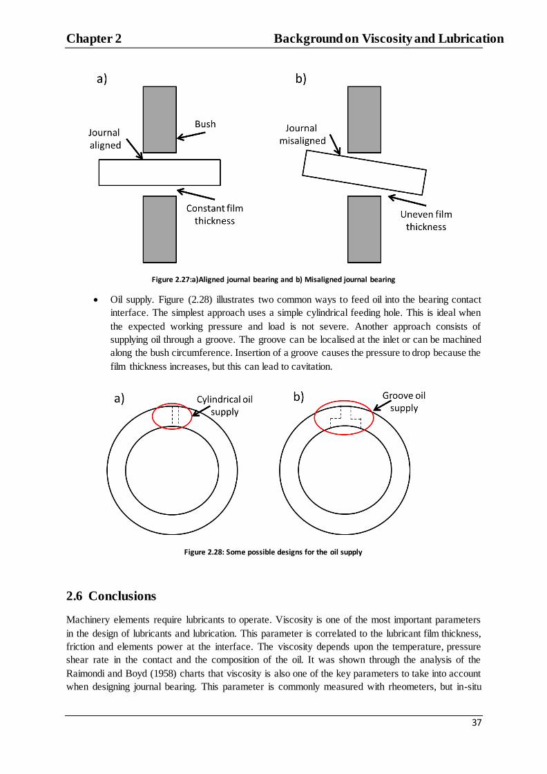
Bearing misalignment. The best bearing design can fail if bearing and shaft are misaligned
when mounted. Figure (2.27) schematically shows an aligned and a misaligned journal
bearing. When the journal and bush are completely aligned the maximum pressure is obtained
at the centre of the bearing. When the bearing is misaligned, the maximum pressure is
obtained where the minimum thickness is encountered. The maximum pressure at
misalignment is higher than the maximum pressure in the aligned case because the film
thickness is less and the friction increases. The bearing, then, operates in non-ideal conditions.
Chapter 2 Background on Viscosity and Lubrication
37
Figure 2.27:a)Aligned journal bearing and b) Misaligned journal bearing
Oil supply. Figure (2.28) illustrates two common ways to feed oil into the bearing contact
interface. The simplest approach uses a simple cylindrical feeding hole. This is ideal when
the expected working pressure and load is not severe. Another approach consists of
supplying oil through a groove. The groove can be localised at the inlet or can be machined
along the bush circumference. Insertion of a groove causes the pressure to drop because the
film thickness increases, but this can lead to cavitation.
Figure 2.28: Some possible designs for the oil supply
2.6 Conclusions
Machinery elements require lubricants to operate. Viscosity is one of the most important parameters
in the design of lubricants and lubrication. This parameter is correlated to the lubricant film thickness,
friction and elements power at the interface. The viscosity depends upon the temperature, pressure
shear rate in the contact and the composition of the oil. It was shown through the analysis of the
Raimondi and Boyd (1958) charts that viscosity is also one of the key parameters to take into account
when designing journal bearing. This parameter is commonly measured with rheometers, but in-situ
Chapter 2 Background on Viscosity and Lubrication
38
measurement with conventional technique is prohibitive. Development of a novel tool to analyse
viscosity in real time can therefore benefit the design of journal bearing and of lubricant additives.

Chapter 3 Background on Ultrasound
39
Chapter 3 Background on Ultrasound
Background on Ultrasound
This chapter presents the background on ultrasound, the technology used in this research work to
measure the lubricant viscosity. The aim of this chapter is to provide the reader with an introduction
to the basic definitions of sound and on the properties of the ultrasonic plane waves. After the basic
definitions and methods, the different ultrasound transducers and measurement setups are introduced.
Finally the reflection of sound from interfaces is analysed in detail.
3.1 Introduction to Ultrasound
The sound is a vibration that propagates throughout a medium by elastic deformation of its particles.
When the vibration occurs at frequencies above the human audible limit ( Hz), it is referred to as
ultrasound. Figure (3.1) reports the range limit for the different type of sound vibrational frequency.
Figure 3.1: Frequency limits for infrasonic, sonic, ultrasonic and hypersonic vibrations (Kinsler and Frey, 2000)
Ultrasonic waves are used in nature by animals, such as bats, for orientation or prey localization.
Since the early twentieth century they have found use also in industry originally for military non-
destructive examination and evaluation of structure (Firestone, 1940). Since then ultrasound has been
used in a wide range of application such as non-destructive examination of structures, medical
applications, fluid chemical analysis, and seismology.
Ultrasound propagates in different modes depending on the sound wave type and source. In this work,
plane wave propagation is studied. Plane waves are defined as constant frequency waves with wave
front propagating as a series of infinite parallel planes (Achenbach, 1973). In this case the particle
deformation can be compressional or transverse. Figure (3.2a) schematically represents a material
particle network at rest as a series of spring and masses to better understand how plane waves
propagate throughout matter. The displacement of the particles is parallel to the wave propagation
when a longitudinal or compressional wave interacts with the particles network, as shown in Figure
(3.2b). On the other hand, the displacement of the particle is normal to the wave propagation when a
shear or transverse wave interacts with the particles network, as shown in Figure (3.2c). When the
wave (either longitudinal or shear) has travelled through the material the particle network returns to
rest in the original configuration as shown in Figure (3.2a) because the deformation due to sound
propagation is considered to be purely elastic. Table (3.1) summarizes the main propagation features
of longitudinal and shear waves.

Chapter 3 Background on Ultrasound
40
Figure 3.2: a) Particle network at rest, b) Longitudinal wave propagation, c) Shear wave propagation
Wave Type Propagation mode Propagation medium Longitudinal The particle displacement is parallel to the
direction of wave propagation Solid, liquid, gas
Shear The particle displacement is normal to the direction of wave propagation
Solid
Table 3.1: Recap of plane waves propagation properties
3.2 Ultrasound and Material Properties
The condition of sound propagation is strictly linked to the material properties. The speed of
propagation in a given material is called speed of sound. With reference to Figure (3.2), the speed of
sound is a function of the inertia of the molecules constituting the particle network and a function of
the stiffness of the springs. The inertia is represented by the density of the particle network and the
stiffness is the bulk modulus in case of compression and the shear modulus in case of transverse
motion. The following formulas report the expressions of the speed of sound for longitudinal and
shear waves:
√
(3.1)
√
(3.2)

Chapter 3 Background on Ultrasound
41
where is the compressional speed of sound, is the transverse speed of sound, is the bulk
modulus, is the material density and is the shear modulus. Equations (3.1) and (3.2) show that the
speed of sound is a characteristic of every material. This quantity can also be related to the vibrational
frequency and to the wavelength through the relation:
𝜆 (3.3)
where c is the speed of sound, f is the frequency and 𝜆 is the wavelength. In many practical
applications the speed of sound is commonly measured through time of flight measurement. This
consists of the measurement of the time needed for a sound wave to propagate though a known
distance as:
(3.4)
Another important acoustic property of materials is the acoustic impedance, z. This property
quantifies how well a sound wave propagates through a determined material. This is defined as the
ratio of the acoustic pressure P, which is the super-pressure the atoms are subjected to when
interacting with a sound wave, and the displacement velocity of the particle, v.
(3.5)
Equation (3.5) can be re-written in terms of material density, , and speed of sound as:
(3.6)
The acoustic impedance is measured in Rayl ( ). Table (3.2) reports the value of acoustic
impedance for common engineering materials.
Material Acoustic Impedance (MRayl) Air 0.0005
Water 1.48
Aluminium 18
Steel 45 Table 3.2: Acoustic impedance of different materials
The values in Table (3.2) highlight that for solid materials the acoustic impedance is much higher than
for liquids and gases. In practice this means that the more compact the particle network constituting a
material is, the easier it is for the sound to travel through it for longer distances.
Ultrasonic wave propagation process is not exempt from energy losses. Figure (3.3) schematically
shows the main source of attenuation of sound energy due to interaction with material: scattering and
absorption.

Chapter 3 Background on Ultrasound
42
Figure 3.3: Schematic representation of the attenuation process for ultrasound wave
Scattering is defined as a redirection of energy due to a material‟s inhomogeneity. When the sound
wave is incident at a material boundary, part of the wave is reflected away from the original
trajectory. Absorption is associated with conversion of ultrasonic vibrational energy into other energy
forms such as thermal energy. The overall attenuation is evaluated in the form of attenuation
coefficient. This can be obtained from the formula:
(3.7)
In equation (3.7) is the amplitude of the ultrasonic wave after a distance d, is the initial
amplitude of the wave and is the attenuation coefficient. Rearranging equation (3.7) the attenuation
coefficient is:
(3.8)
attenuation in metallic materials is usually low, allowing investigation of thick specimens, while
propagation in softer material like plastics is much more attenuated. The attenuation coefficient is
highly dependent on the temperature and the stress state. As result of this it is recommended to
determine the attenuation coefficient experimentally rather than rely on literature tables.
3.3 Ultrasonic Transducers
3.3.1 The Piezoelectric Effect
Generation and reception of sound waves is commonly achieved by the so-called piezoelectric effect.
This is a property possessed by a class of materials, the piezoelectric materials, that was discovered by
the Curie brothers (1880). They noted that when an electric potential was applied to a piezoelectric
crystal cut in a certain direction, a deformation or vibration occurs. On the other hand, when the
crystal was deformed an electric charge is produced. The possibility of generating ultrasonic waves
and converting the vibration into an electric signal allows the production of ultrasonic transducers for
non-destructive examination. Originally these transducers were made with a single barium titanate
quartz. However, in the 1950s these where replaced with ceramic plate made of lead zirconate titanate

Chapter 3 Background on Ultrasound
43
or PZT that are still widely used today. Ceramic materials are cheaper and do not need to be cut in a
certain direction to allow the piezoelectric effect to take place. This is an advantage because PZT can
then come in different shape (rectangular, circular, rod and so on) depending on the desired
application.
3.3.2 Ultrasonic Transducer Type
Ultrasonic transducers can be used as transmitters or receivers of the ultrasonic wave. The bare crystal
can be used as stand-alone pulsing-receiving unit or it can be incorporated in a probe. For industrial
applications the frequency of the ultrasonic transducer ranges from 0.5-50 MHz. The schematic
representation of an ultrasonic commercial probe is shown in Figure (3.4). The main elements
constituting a commercially assembled ultrasonic probe are the:
Piezoelectric element
External housing
Backing material
Wear plate
Electrical connection and connector
Figure 3.4: Schematic representation of an ultrasonic probe
The external housing is usually cylindrical, and together with the wear plate protects the active
element from wear and external agents. The backing material damps the vibration of the piezoelectric
element inner face allowing the transmission of a short pulse rather than a continuous signal.
Commercial probes are divided into contact and immersion transducers, as shown in Figure (3.5a) and
(3.5b).
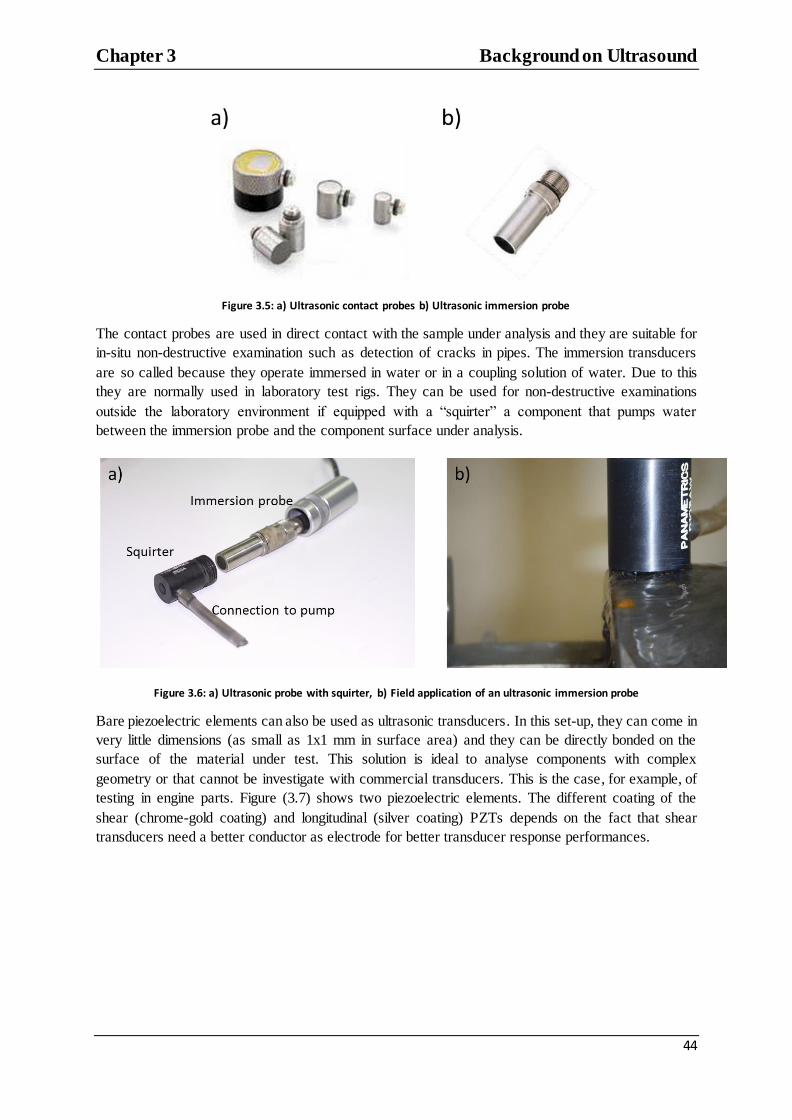
Chapter 3 Background on Ultrasound
44
Figure 3.5: a) Ultrasonic contact probes b) Ultrasonic immersion probe
The contact probes are used in direct contact with the sample under analysis and they are suitable for
in-situ non-destructive examination such as detection of cracks in pipes. The immersion transducers
are so called because they operate immersed in water or in a coupling solution of water. Due to this
they are normally used in laboratory test rigs. They can be used for non-destructive examinations
outside the laboratory environment if equipped with a “squirter” a component that pumps water
between the immersion probe and the component surface under analysis.
Figure 3.6: a) Ultrasonic probe with squirter, b) Field application of an ultrasonic immersion probe
Bare piezoelectric elements can also be used as ultrasonic transducers. In this set-up, they can come in
very little dimensions (as small as 1x1 mm in surface area) and they can be directly bonded on the
surface of the material under test. This solution is ideal to analyse components with complex
geometry or that cannot be investigate with commercial transducers. This is the case, for example, of
testing in engine parts. Figure (3.7) shows two piezoelectric elements. The different coating of the
shear (chrome-gold coating) and longitudinal (silver coating) PZTs depends on the fact that shear
transducers need a better conductor as electrode for better transducer response performances.
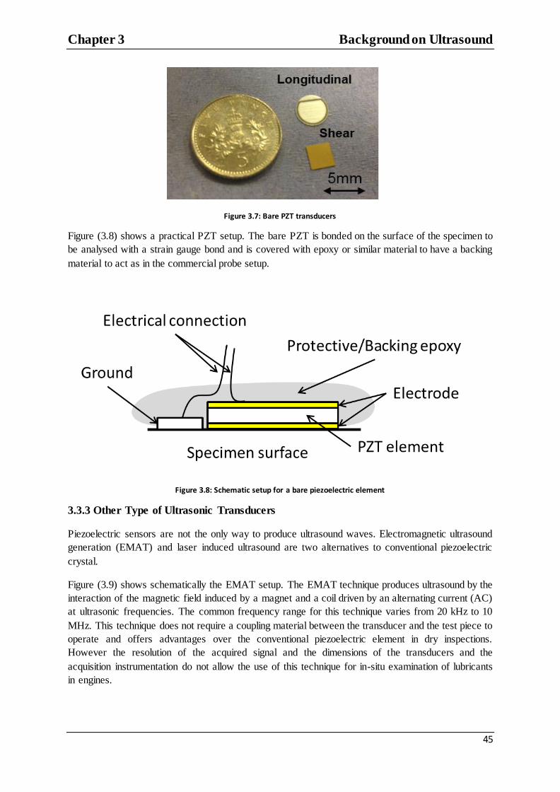
Chapter 3 Background on Ultrasound
45
Figure 3.7: Bare PZT transducers
Figure (3.8) shows a practical PZT setup. The bare PZT is bonded on the surface of the specimen to
be analysed with a strain gauge bond and is covered with epoxy or similar material to have a backing
material to act as in the commercial probe setup.
Figure 3.8: Schematic setup for a bare piezoelectric element
3.3.3 Other Type of Ultrasonic Transducers
Piezoelectric sensors are not the only way to produce ultrasound waves. Electromagnetic ultrasound
generation (EMAT) and laser induced ultrasound are two alternatives to conventional piezoelectric
crystal.
Figure (3.9) shows schematically the EMAT setup. The EMAT technique produces ultrasound by the
interaction of the magnetic field induced by a magnet and a coil driven by an alternating current (AC)
at ultrasonic frequencies. The common frequency range for this technique varies from 20 kHz to 10
MHz. This technique does not require a coupling material between the transducer and the test piece to
operate and offers advantages over the conventional piezoelectric element in dry inspections.
However the resolution of the acquired signal and the dimensions of the transducers and the
acquisition instrumentation do not allow the use of this technique for in-situ examination of lubricants
in engines.
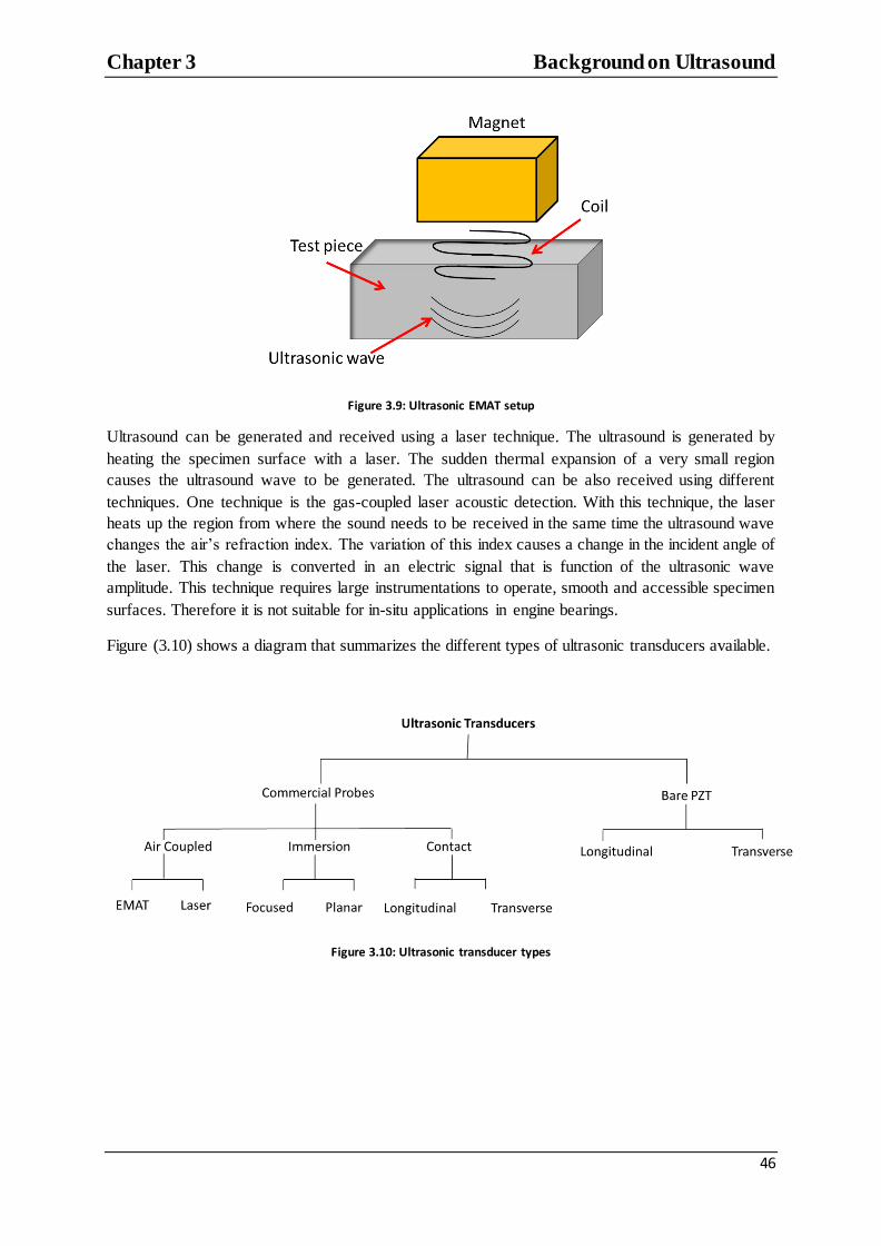
Chapter 3 Background on Ultrasound
46
Figure 3.9: Ultrasonic EMAT setup
Ultrasound can be generated and received using a laser technique. The ultrasound is generated by
heating the specimen surface with a laser. The sudden thermal expansion of a very small region
causes the ultrasound wave to be generated. The ultrasound can be also received using different
techniques. One technique is the gas-coupled laser acoustic detection. With this technique, the laser
heats up the region from where the sound needs to be received in the same time the ultrasound wave
changes the air‟s refraction index. The variation of this index causes a change in the incident angle of
the laser. This change is converted in an electric signal that is function of the ultrasonic wave
amplitude. This technique requires large instrumentations to operate, smooth and accessible specimen
surfaces. Therefore it is not suitable for in-situ applications in engine bearings.
Figure (3.10) shows a diagram that summarizes the different types of ultrasonic transducers available.
Figure 3.10: Ultrasonic transducer types
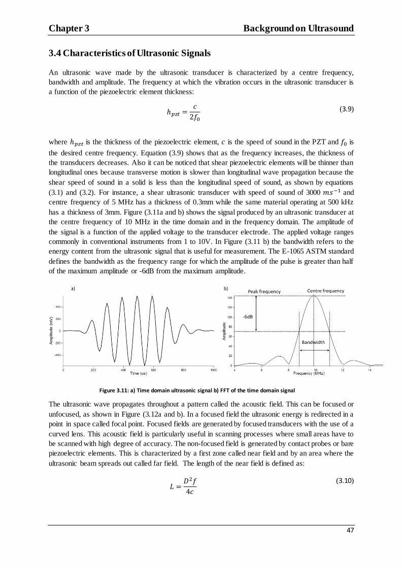
Chapter 3 Background on Ultrasound
47
3.4 Characteristics of Ultrasonic Signals
An ultrasonic wave made by the ultrasonic transducer is characterized by a centre frequency,
bandwidth and amplitude. The frequency at which the vibration occurs in the ultrasonic transducer is
a function of the piezoelectric element thickness:
(3.9)
where is the thickness of the piezoelectric element, c is the speed of sound in the PZT and is
the desired centre frequency. Equation (3.9) shows that as the frequency increases, the thickness of
the transducers decreases. Also it can be noticed that shear piezoelectric elements will be thinner than
longitudinal ones because transverse motion is slower than longitudinal wave propagation because the
shear speed of sound in a solid is less than the longitudinal speed of sound, as shown by equations
(3.1) and (3.2). For instance, a shear ultrasonic transducer with speed of sound of 3000 and
centre frequency of 5 MHz has a thickness of 0.3mm while the same material operating at 500 kHz
has a thickness of 3mm. Figure (3.11a and b) shows the signal produced by an ultrasonic transducer at
the centre frequency of 10 MHz in the time domain and in the frequency domain. The amplitude of
the signal is a function of the applied voltage to the transducer electrode. The applied voltage ranges
commonly in conventional instruments from 1 to 10V. In Figure (3.11 b) the bandwidth refers to the
energy content from the ultrasonic signal that is useful for measurement. The E-1065 ASTM standard
defines the bandwidth as the frequency range for which the amplitude of the pulse is greater than half
of the maximum amplitude or -6dB from the maximum amplitude.
The ultrasonic wave propagates throughout a pattern called the acoustic field. This can be focused or
unfocused, as shown in Figure (3.12a and b). In a focused field the ultrasonic energy is redirected in a
point in space called focal point. Focused fields are generated by focused transducers with the use of a
curved lens. This acoustic field is particularly useful in scanning processes where small areas have to
be scanned with high degree of accuracy. The non-focused field is generated by contact probes or bare
piezoelectric elements. This is characterized by a first zone called near field and by an area where the
ultrasonic beam spreads out called far field. The length of the near field is defined as:
(3.10)
Figure 3.11: a) Time domain ultrasonic signal b) FFT of the time domain signal

Chapter 3 Background on Ultrasound
48
where L is the near field length, D is the transducer diameter, f is the frequency and c is the speed of
sound in the medium. The near field is characterized by superposition of waves generated by and
reflected to the transducer. It is good practice to work with signals acquired at the end of the near field
for maximum amplitude energy and minimum noise.
Figure 3.12: a) Planar transducer acoustic field, b) Focused transducer acoustic field
3.5 Transducers Arrangements
Figure (3.13) presents the two main ultrasonic set-up techniques: through-transmission and pulse
echo.
Figure 3.13: a) Through transmission method, b) Pulse echo method
Figure (3.13a) shows the setup of the through-transmission technique. In this case one transducer
emits the ultrasonic wave while the second transducer located on the other side of the specimen
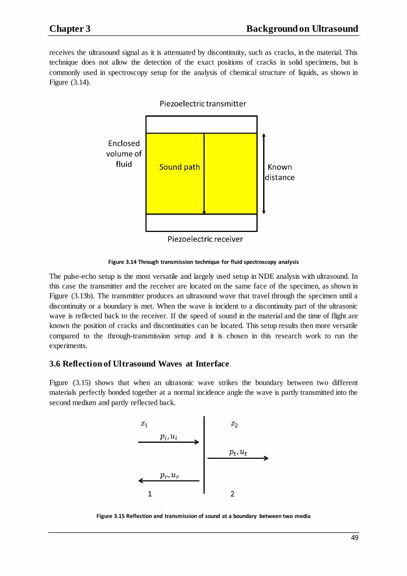
Chapter 3 Background on Ultrasound
49
receives the ultrasound signal as it is attenuated by discontinuity, such as cracks, in the material. This
technique does not allow the detection of the exact positions of cracks in solid specimens, but is
commonly used in spectroscopy setup for the analysis of chemical structure of liquids, as shown in
Figure (3.14).
Figure 3.14 Through transmission technique for fluid spectroscopy analysis
The pulse-echo setup is the most versatile and largely used setup in NDE analysis with ultrasound. In
this case the transmitter and the receiver are located on the same face of the specimen, as shown in
Figure (3.13b). The transmitter produces an ultrasound wave that travel through the specimen until a
discontinuity or a boundary is met. When the wave is incident to a discontinuity part of the ultrasonic
wave is reflected back to the receiver. If the speed of sound in the material and the time of flight are
known the position of cracks and discontinuities can be located. This setup results then more versatile
compared to the through-transmission setup and it is chosen in this research work to run the
experiments.
3.6 Reflection of Ultrasound Waves at Interface.
Figure (3.15) shows that when an ultrasonic wave strikes the boundary between two different
materials perfectly bonded together at a normal incidence angle the wave is partly transmitted into the
second medium and partly reflected back.
Figure 3.15 Reflection and transmission of sound at a boundary between two media

Chapter 3 Background on Ultrasound
50
In Figure (3.15) is the incident wave pressure and is the incident wave velocity, while the
subscripts t and r refer to the transmitted and reflected waves respectively. By continuity of pressure
and velocity at the boundary:
and (3.11)
Rearranging equation (3.11) gives:
(3.12)
From the definition of acoustic impedance (equation (3.5)):
and
and
(3.13)
where the sign depends on the arbitrary convention on the positive direction of the propagation axis.
This means that the terms on the right in the equation (3.12) is the acoustic impedance of the second
medium, while the particle velocities on the left hand side terms can be written in terms of acoustic
impedance and acoustic pressure using the expression (3.13). Rearranging in this way equation (3.12)
becomes:
(3.14)
The amount of energy reflected is calculated in the form of amplitude reflection coefficient. This is a
non-dimensional factor that states the percentage of ultrasonic signal amplitude that is reflected from
an interface as:
(3.15)
Substituting equation (3.15) in equation (3.14), it is possible to obtain an expression of the reflection
coefficient in terms of acoustic impedance as:
(3.16)
In the same way, the transmitted amplitude is calculated in the form of amplitude transmission
coefficient as:
(3.17)
When the second medium is a liquid only longitudinal wave can be transmitted while shear wave can
propagate only for a very short distance, as shown in Figure (3.16).

Chapter 3 Background on Ultrasound
51
Figure 3.16: a) Propagation of longitudinal sound wave at solid-liquid interface, b) Propagation of shear sound wave at solid-liquid interface
The propagation distance that a shear wave can withstand in a fluid is called penetration depth and is
calculated as (Buckin, 2001):
√
(3.18)
In equation (3.18) is the penetration depth, is the viscosity, and is the density of the fluid.
Figure (3.17) shows what happens when an ultrasonic waves is incident to a solid-solid and to a solid-
liquid boundary at a non-normal incidence angle.

Chapter 3 Background on Ultrasound
52
Figure 3.17: Reflection and transmission of ultrasound longitudinal (a) and shear (b) waves at solid-solid boundary and
reflection and transmission of ultrasound longitudinal (c) and shear (d) waves at solid-liquid boundary at an angle different from normal incidence
In the case of a longitudinal wave and in the case of solid-solid boundary the reflected and transmitted
resultants are affected by mode conversion, meaning that both longitudinal and transverse resultants
are produced. The angle at which the longitudinal and the transverse wave are produced can be
calculated using the Snell‟s law of reflection:
𝜃
𝜃
(3.19)
where is the speed of sound of the incident wave (either longitudinal or shear) and is the speed
of sound in the medium where reflection or transmission occurs, 𝜃 is sine of the angle of
incidence and 𝜃 is the angle at which reflection or transmission occurs. In the case of
longitudinal wave incident to a solid-liquid boundary, the reflected wave will be affected by mode
conversion, while in the liquid medium only a longitudinal wave will propagate. The angles of
reflection and transmission can be calculated again using the Snell‟s law. In case a shear wave is
incident to a solid-solid boundary, no mode conversion happens and the reflection and transmission
angle is calculated again with equation (3.17). Finally, Figure (3.17d) shows that when a shear wave
is incident to a solid-liquid boundary only a shear wave is reflected.
The reflection coefficient is the most important ultrasonic measurable parameter because it can be
correlated to many material properties. In the case of shear waves, the reflected energy from a solid-
liquid layer can be directly correlated with the liquid viscosity, as shown in the latter chapters.

Chapter 3 Background on Ultrasound
53
3.6.1 Reflection and Transmission in a Three-Layered System
Figure (3.18) shows the propagation of an ultrasonic wave through two media into a third one. This is
the case of propagation of longitudinal or shear waves when at least medium one and two are solid or
the case of propagation of a longitudinal wave when media two and three are liquids.
Figure 3.18 Sound transmission and reflection in a three layered system
The boundary conditions for the situation depicted in Figure (3.17) are continuity of shear
displacement and shear force at the two boundaries and . If the displacement and
the consequent pressure field are supposed to be sinusoidal, the following relation applies:
(3.20)
where P is a constant, k is the wave number in the medium considered and the subscript x refers to
any incident or reflection subscript for the different wave component in Figure (3.17). At the
application of the continuity displacement boundary condition gives:
(3.21)
where k is the wave number in the medium considered. Since it is supposed that then equation
(3.21) becomes:
(3.22)
The second boundary condition at states that the force ( ⁄ ) is continuous so:
(3.23) If equation (3.23) is divided by ω and remembering that 𝜔⁄ , then the equation becomes:
(3.24) Similarly the application of the same boundary conditions at gives for the displacement
continuity:
(3.25) and for the force continuity:
(
) (3.26)
x
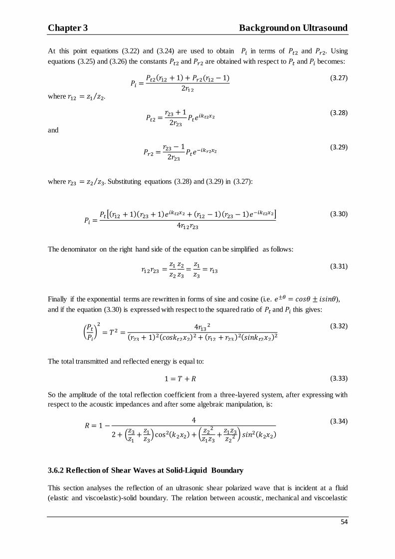
Chapter 3 Background on Ultrasound
54
At this point equations (3.22) and (3.24) are used to obtain in terms of and . Using
equations (3.25) and (3.26) the constants and are obtained with respect to and becomes:
(3.27)
where ⁄ .
(3.28)
and
(3.29)
where ⁄ . Substituting equations (3.28) and (3.29) in (3.27):
[ ]
(3.30)
The denominator on the right hand side of the equation can be simplified as follows:
(3.31)
Finally if the exponential terms are rewritten in forms of sine and cosine (i.e. 𝜃 𝜃),
and if the equation (3.30) is expressed with respect to the squared ratio of and this gives:
(
)
(3.32)
The total transmitted and reflected energy is equal to:
(3.33)
So the amplitude of the total reflection coefficient from a three-layered system, after expressing with
respect to the acoustic impedances and after some algebraic manipulation, is:
(
) (
)
(3.34)
3.6.2 Reflection of Shear Waves at Solid-Liquid Boundary
This section analyses the reflection of an ultrasonic shear polarized wave that is incident at a fluid
(elastic and viscoelastic)-solid boundary. The relation between acoustic, mechanical and viscoelastic

Chapter 3 Background on Ultrasound
55
parameters obtained in this chapter is the basis of the ultrasonic analytical model described in chapters
4 and 5. The analysis starts by considering the interaction of a shear wave with an element of fluid as
shown in Figure (3.19).
Figure 3.19: Interaction of a shear wave stress with a fluid element
The equation of motion for a fluid element under the stress is:
(
)
(3.35)
where is the particle displacement. By defining the shear modulus as and
gives:
(
)
(3.36)
This is the wave equation in general form in case of shear stress applied to the element of fluid shown
in Figure (3.18). For sinusoidal displacement the solution of this equation is:
(3.37)
In the last equation √
is the speed of the shear wave. In the case where the wave is propagating
into a solid the value of G would be a real value, and this leads to the relation of the acoustic
impedance and sound speed presented in equation (3.6). For a purely viscous (Newtonian) fluid G is
90 degrees out of phase with the strain and this means that the shear modulus is composed just by the
imaginary component. From Newton‟s law, and:

Chapter 3 Background on Ultrasound
56
𝜔
(3.38)
In a real viscoelastic fluid, the complex shear modulus is composed of a real and an imaginary part:
(3.39)
where the real part is called the storage modulus, while the imaginary component is called loss
modulus. Figure (3.20) helps understanding what the shear modulus represents for viscoelastic fluids
with a simple experiment.
Figure 3.20: The rotational viscometer analogy to show fluid behaviour under oscillation
In this figure, the cup contains a fluid and is connected to a motor that oscillates with sinusoidal
motion. Inside the cup and in contact with the fluid, is a cylinder that rotates passively with the fluid.
For instance, if the fluid is replaced with a solid the cup and the cylinder would oscillate in phase as
shown in Figure (3.19). Alternatively, if a completely viscous fluid is in the cup the oscillation would
be 90° out of phase. For real viscoelastic fluids the oscillation is partly in phase, and partly out of
phase. As a consequence also the resistance offered by the fluid to the motion will be partly in phase
and partly out of phase. When defining the shear modulus of a fluid the real component, or the storage
modulus, is a measure of the material‟s ability to store elastic energy, while the out of phase
component, or loss modulus, is related to the viscosity. The shear modulus is then a very important
parameter to define the viscoelastic behaviour of fluids and polymers.
The shear modulus can be related to the impedance of a viscoelastic fluid. By definition the acoustic
impedance is the ratio between the acoustic load and the displacement on the fluid element:
(3.40)

Chapter 3 Background on Ultrasound
57
Substituting equation (3.35) in equation (3.38) a direct correlation between shear acoustic impedance
and shear modulus is obtained:
𝜔
(3.41)
and the value of fluid impedance may be correlated with the shear reflection coefficient in the same
way as defined in equation (3.16). In this case the reflection coefficient R is a complex value because
is complex and can be written in terms of modulus and phase as:
| | (3.42)
where | | is the reflection coefficient modulus and is the reflection coefficient phase . From
equation (3.39) it can be noticed that the value of the fluid impedance is a complex value that can be
expressed as and so the reflection coefficient may be written in the following form:
√
√
(3.43)
The modulus of the complex reflection coefficient can be obtained as:
| | √
(3.44)
where:
√ (3.45)
and
( √ ) (3.46)
Equation (3.44) can be simplified in case of Newtonian fluid. In this particular case =0, 𝜔
and and become:
√ 𝜔
(3.47)
Equation (3.47) shows the relation between the viscosity and the shear modulus in the terms of
and . Substituting equation (3.47) in equation (3.44) it is possible to obtain a relation between
viscosity and reflection coefficient. This relation is implemented in chapter 4 to obtain the relation
between the viscosity of a Newtonian fluid and the reflection coefficient at a solid-liquid boundary. In
chapter 5 the hypothesis of Newtonian fluid is overcome and the relation between reflection
coefficient and viscosity is solved in case of Non-Newtonian Maxwell fluids.

Chapter 3 Background on Ultrasound
58
3.7 Conclusions
Ultrasonic methods are ideal for non-invasive testing. Different transducers types are available, but
the bare piezoelectric transducers are ideal for the analysis of lubricants in machinery components.
This is because they can be miniaturized to fit machinery components with geometries that are
difficult to access with conventional techniques. This is the case for engine parts like journal bearings.
The pulse-echo transducers arrangement allows the propagation of an ultrasonic wave through a
component and the analysis of the reflected echo from the solid-liquid boundary of a lubricated
contact. The amplitude of the reflected echo is measured as reflection coefficient. This is a quantity
that can be directly measured experimentally (see chapter 6) and that can be directly correlated to the
fluid viscosity. The reflection coefficient, in fact, is a function of the acoustical and mechanical
properties of the solid where the transducers are bonded and the viscoelastic characteristic of the
liquid layer. In chapters 4 and 5 the correlation between the reflection coefficient and the viscosity is
studied to obtain an analytical model for the correlation of viscosity with the experimentally measured
reflection coefficient.

Chapter 4 Literature Review
59
Chapter 4
Literature Review This chapter presents the literature review on liquid viscosity measurement by means of ultrasonic
plane waves. The purpose of this review is to provide the knowledge of the current state of the art in
ultrasonic plane waves viscometry. Several techniques have been developed to study viscosity with
ultrasound. The first part of the literature review analyses these methods. They may be recapped in the
following categories: crystal and rod resonators, the speed of sound and attenuation techniques,
spectroscopy and the reflectance technique. In this review the advantages, applications and the
limitations of each method are analysed. The second part of the literature reports how these
techniques have been used to analyse lubricating oils. The review provides also a comparison between
the ultrasonic viscometers and the conventional viscometers. Finally, the considerations on the limits
of the literature methods are used to point out the direction undertaken in this research to design a
novel ultrasonic viscometer for in-situ applications in journal bearings.
4.1 The Crystal Resonator
The pioneer of the use of ultrasonic techniques for measuring viscosity was Mason (1948). In his
innovative work Mason described the possibility of studying the viscoelastic characteristic of liquid
mixtures by shearing them quickly enough to analyse ultrasonic waves elastic effect on solid particles
dispersed in the liquid. Mason‟s work is divided both in the analysis of resonance quartz peak
variation and in the analysis of the reflection coefficient from a solid-liquid boundary. Figure (4.1)
shows the setup implemented by Mason. Every piezoelectric material has a resonance peak at a
certain frequency and Mason noticed that if a quartz crystal was immersed into a liquid the frequency
peak was shifted. The analysis of the resonance peak shifts in the quartz-liquid system was used to
calculate the viscoelastic properties of different fluid mixtures. Mason‟s equipment pulsed a
piezoelectric (PZT) crystal at 500 kHz and analysed the response with good agreement to theoretical
data fluids with a value of shear viscosity up to 10 mPas.
Figure 4.1: Mason’s reflectance set-up
Mason‟s resonating quartz viscometer is still used in industry. The resonating crystal approach is
applied, for example, to analyse the viscosity of curing epoxy in composite materials (Bujard, 1989).

Chapter 4 Literature Review
60
The resonating quartz technique is also used to produce modern acoustic microbalances (Eggers and
Funk, 1987).
Figure 4.2 Frequency response from quartz-air system and from quartz fluid system in the frequency shift technique
4.2 The Resonating Plate/Rod Woodward (1953) and Rich and Roth (1953) developed in parallel two vibrational viscometers based
on Mason‟s resonance frequency shift principle. This was the first attempt to build an ultrasonic
viscometer to be used on-site for industrial characterization of lubricants. The Woodward viscometer
correlated the damping experienced by a vibrating plate driven by a piezoelectric crystal immersed in
a viscous fluid. Similarly, the so called ultra-viscoson by Rich and Roth, shown in Figure (4.3),
operated with a magnetostrictive strip or cylindrical rod driven by a piezoelectric sensor that was used
to produce transverse elastic waves guided to interact with the fluid sample of interest. This work is of
particular importance because for the first time the piezoelectric transducer was not in direct contact
with the fluid being analysed. The resonating plate viscometer consisted of a metal strip that was
immerged in the liquid and vibrated at a desired frequency (in the range 0.2-2MHz). The vibration of
the strip into the liquid was compared to the one in a reference volume (e.g. air). The vibration in the
liquid was damped by the vibration in air. This damping was correlated to the viscosity of the liquid.
This viscometer cannot be used to analyse thin layers of lubricant because of the dimensions of the
probe, so the implementation to real time and on site application was, in fact, limited to the analysis of
fluids in barrels or pipes. Kim and Bau (1988) refined this viscometer at low operational frequencies
(50 kHz). Kauzlarich (1996) used the same operating principle at higher frequencies (2.5 MHz) to
obtain a patent for an ultrasonic viscometer for general fluid characterization. The main limitation of
the resonating plate is that the waveguide cannot be used to analyse the thin films that are present in
machinery lubricated layers.

Chapter 4 Literature Review
61
Figure 4.3: Schematic representation of the resonating waveguide. The vibration of the strip is damped when it is
submerged in the fluid sample. The damping is correlated to the viscosity of the fluid (Woodward, 1953)
Figure 4.4: Archive image of the Ultra-Viscoson from Roth and Rich (1953)
4.3 Reflectance Methodologies
Mason (1948) described in his ground-breaking work the possibility of using the reflection of shear
ultrasound waves from the piezoelectric-fluid interface to measure viscosity. Following Mason‟s
work, different approaches based on the reflection coefficient analysis have been developed and
nowadays different reflection coefficient techniques are at the heart of modern ultrasonic viscometers.
Figure (4.5) shows schematically the set-up for the analysis of the reflection of shear waves at a solid-
liquid boundary. The ultrasonic pulser and receiver in Figure (4.5b) can be represented by any kind of
transducer described in sections 3.2 and 3.3.
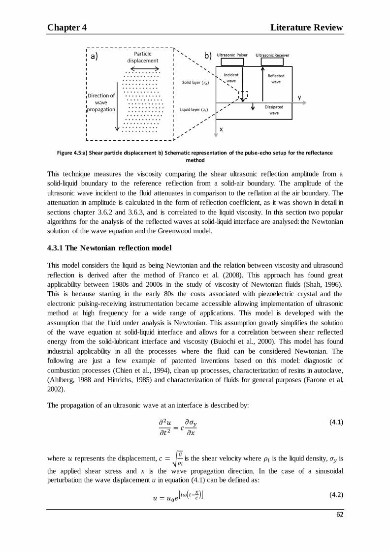
Chapter 4 Literature Review
62
Figure 4.5:a) Shear particle displacement b) Schematic representation of the pulse-echo setup for the reflectance method
This technique measures the viscosity comparing the shear ultrasonic reflection amplitude from a
solid-liquid boundary to the reference reflection from a solid-air boundary. The amplitude of the
ultrasonic wave incident to the fluid attenuates in comparison to the reflation at the air boundary. The
attenuation in amplitude is calculated in the form of reflection coefficient, as it was shown in detail in
sections chapter 3.6.2 and 3.6.3, and is correlated to the liquid viscosity. In this section two popular
algorithms for the analysis of the reflected waves at solid-liquid interface are analysed: the Newtonian
solution of the wave equation and the Greenwood model.
4.3.1 The Newtonian reflection model
This model considers the liquid as being Newtonian and the relation between viscosity and ultrasound
reflection is derived after the method of Franco et al. (2008). This approach has found great
applicability between 1980s and 2000s in the study of viscosity of Newtonian fluids (Shah, 1996).
This is because starting in the early 80s the costs associated with piezoelectric crystal and the
electronic pulsing-receiving instrumentation became accessible allowing implementation of ultrasonic
method at high frequency for a wide range of applications. This model is developed with the
assumption that the fluid under analysis is Newtonian. This assumption greatly simplifies the solution
of the wave equation at solid-liquid interface and allows for a correlation between shear reflected
energy from the solid-lubricant interface and viscosity (Buiochi et al., 2000). This model has found
industrial applicability in all the processes where the fluid can be considered Newtonian. The
following are just a few example of patented inventions based on this model: diagnostic of
combustion processes (Chien et al., 1994), clean up processes, characterization of resins in autoclave,
(Ahlberg, 1988 and Hinrichs, 1985) and characterization of fluids for general purposes (Farone et al,
2002).
The propagation of an ultrasonic wave at an interface is described by:
(4.1)
where represents the displacement, √
is the shear velocity where is the liquid density, is
the applied shear stress and x is the wave propagation direction. In the case of a sinusoidal
perturbation the wave displacement u in equation (4.1) can be defined as:
* (
)+
(4.2)
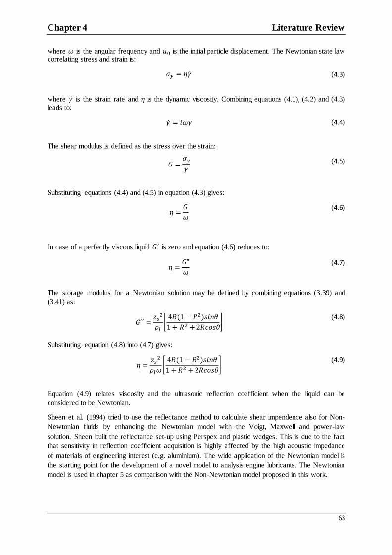
Chapter 4 Literature Review
63
where 𝜔 is the angular frequency and is the initial particle displacement. The Newtonian state law correlating stress and strain is:
(4.3)
where is the strain rate and is the dynamic viscosity. Combining equations (4.1), (4.2) and (4.3) leads to:
𝜔 (4.4)
The shear modulus is defined as the stress over the strain:
(4.5)
Substituting equations (4.4) and (4.5) in equation (4.3) gives:
𝜔
(4.6)
In case of a perfectly viscous liquid is zero and equation (4.6) reduces to:
𝜔
(4.7)
The storage modulus for a Newtonian solution may be defined by combining equations (3.39) and
(3.41) as:
* 𝜃
𝜃+
(4.8)
Substituting equation (4.8) into (4.7) gives:
𝜔* 𝜃
𝜃+
(4.9)
Equation (4.9) relates viscosity and the ultrasonic reflection coefficient when the liquid can be
considered to be Newtonian.
Sheen et al. (1994) tried to use the reflectance method to calculate shear impendence also for Non-
Newtonian fluids by enhancing the Newtonian model with the Voigt, Maxwell and power-law
solution. Sheen built the reflectance set-up using Perspex and plastic wedges. This is due to the fact
that sensitivity in reflection coefficient acquisition is highly affected by the high acoustic impedance
of materials of engineering interest (e.g. aluminium). The wide application of the Newtonian model is
the starting point for the development of a novel model to analysis engine lubricants. The Newtonian
model is used in chapter 5 as comparison with the Non-Newtonian model proposed in this work.

Chapter 4 Literature Review
64
Figure 4.6 Kasolang-Dwyer Joyce set-up for measuring viscosity and film thickness in Journal bearings: it can be noticed the shear sensor to be inserted in the shaft (Kasolang and Dwyer Joyce, 2011)
4.3.2 The Greenwood Model
Greenwood (2002) developed another reflection coefficient based technique. This model can be easily
obtained from the definition of acoustic impedance for Newtonian fluids as it has been shown in the
work of Kasolang and Dwyer-Joyce(2011). This methodology has the advantage of being independent
of the film thickness and the reflection coefficient phase, but its applicability is still limited to
Newtonian fluids in the viscosity range 5-600 mPas.
The equation that correlates the viscosity of a fluid layer and the ultrasonic reflection coefficient is
derived starting from the most general definition of acoustic impedance for a viscoelastic fluid:
(4.10)
From the definition of viscosity the shear stress is proportional to the shear strain and so:
(4.11)
Combining equation (4.11) and equation (4.1), and if equation (4.1) is solved with the limitation that
the displacement is sinusoidal, a solution for u is obtained in the form:
(4.12)
Where k’ is defined by Greenwood et al. (2002) and it is solution of equation (4.1) only if it is equal
to:
(𝜔
)
(4.13)

Chapter 4 Literature Review
65
Finally substituting equation (4.13) in equations (4.11) and (4.10) gives the definition of acoustic
impedance:
(𝜔
) (4.14)
By equating the real parts of the reflection coefficient equation (3.14) and the real part of equation
(4.14) the fluid viscosity value is obtained in terms of reflection coefficient:
( (
𝜔)
(
))
(4.15)
Equation (4.15) presents a simplified approach to the problem with respect to equation (4.9) as only
the modulus, and not phase, of the reflection coefficient is needed to calculate shear viscosity. This
model has been studied and implemented for its simplicity and the good accuracy of the results
obtained. The weakness of this model is that it can be used only to study Newtonian fluids.
4.4 The Attenuation Method
Longitudinal plane waves can be used to measure viscosity as well. The use of a longitudinal stress
instead of a shear stress allows the measurement of a quantity called compressional viscosity. This is a
measure of the resistance of the fluid particle network to a normal stress. The use of longitudinal
waves is at the base of the attenuation method. Dukhin (2009) correlated the attenuation of an
ultrasonic wave to the longitudinal viscosity through the relation:
𝜔 (4.16)
The attenuation coefficient was measured experimentally using equation (3.8). In this equation the
value of speed of sound is obtained through time of flight measurement as described in section (3.2)
in equation (3.4). Figure (4.7) shows the conventional set-up to measure the speed of sound using the
time of flight technique.
Figure 4.7: Schematic setup of the attenuation and time of flight technique test cell
The time of flight measurement technique consists in measuring the time that takes to an ultrasonic
longitudinal wave to travel through a path of known length that is filled with the liquid. The speed of

Chapter 4 Literature Review
66
sound in a liquid can be related to many fluid properties. An example of the time of flight
methodology is reported in the work of Greenwood (2003). In this work a simultaneous measurement
of density and viscosity was made by taking into account the possibility of measuring accurately the
speed of sound in the fluid layer under examination by knowing the time of flight in the layer. The
weakness of this model is that it can be implemented only for fluid in a bulk. The Greenwood model
for viscosity measurement by means of time of flight measurement found applicability in the
characterization of slurry and the range of viscosity covered is 4 to 940 mPas at the frequency of 2.25
MHz.
The attenuation coefficient method is based on the same principle of the time of flight method. If the
time of flight is known then the attenuation coefficient can be calculated through equation (3.8). The
attenuation coefficient can be correlated to the fluid composition and to the longitudinal viscosity. Ju,
Gotlieb et al. (2010) followed Dukhin‟s work and demonstrated that using the set-up shown in Figure
(4.7) it is possible to correlate the attenuation of the sound wave that travels through the liquid with
the sample viscosity. In this case the viscosity will be a combination of the shear viscosity and the
longitudinal viscosity, defined as the resistance of the fluid to normal stress. Shear viscosity,
longitudinal viscosity and attenuation can be correlated through:
𝜔
(
)
(4.17)
The method has proven to be ideal for the investigation of fluids flowing through a pipe (Augenstein
et al., 1999), but it is not suitable for application in the analysis of thin layer of fluid because the
method is based on the time of flight measurement.
4.5 Ultrasonic Spectroscopy Methods
Recently, Kaatze (2001) developed a shear spectroscopy approach to measure viscosity of low
viscosity fluids. Figure (4.8) shows the set-up developed by Kaatze for spectroscopy measurements of
the liquid shear viscosity.
Figure 4.8: Spectroscopy ultrasonic viscometer (Kaatze, 2001). The fluid sample (9) viscosity is analysed using a
piezoelectric crystal (5).
The set-up is, again, very similar to the one proposed by Mason. An AT-cut quartz in contact with the
fluid and oscillated transversely. The oscillation was damped by the presence of the liquid and the
damping was correlated to the liquid viscosity. This damping corresponded also to a shift of the
resonance frequency. The shift is calculated as:
(4.18)

Chapter 4 Literature Review
67
where is the frequency shift, is the immaginary part of the shear acoustic impedance, is the
real part of the shear impedance of the unloaded quartz and is the resonance frequency of the
unloaded quartz, 2 MHz in the experiment by Kaatze. Combining equations (4.18) and equation
(3.41) Kaatze calculated the complex viscosity coefficients as:
and
(4.19)
Using the shift of the frequency spectrum between 1 and 150 MHz Kaatze measured the viscosity at a
wide range of frequencies. Figure (4.9) shows the results obtained by Kaatze.
Figure 4.9: Spectroscopy viscosity measurement by Kaatze. (Kaatze, 2001)
The results are in good agreement for the real component of the viscosity, but the experimental error
is high for the imaginary component (up to over 20 %). This method has not found applicability in
real time processes as for an ultrasonic spectroscopy approach it is necessary to contain the lubricant
of interest into a perfectly machined test cell, as shown in Figure (4.9). This is, in fact, a limitation in
industrial processes. In other experiments Kaatze (2001) used a combination of longitudinal and shear
wave to analyse a wide variety of fluid samples mechanical and chemical properties. The shear
viscosity of a series of samples in the range 6-120 MHz is obtained with a technique based on the
quartz resonator technique. The complex shear viscosity spectrum in this case was used to find the
relaxation frequency and the results were compared with the classical longitudinal wave based
techniques.
4.6 Ultrasonic Resonator to Analyse Lubricating Oils
One of the limitations of the previously described methodologies is that most of them consider the
fluid as perfectly viscous. In the analysis of lubrication regimes this assumption is not valid anymore.
Dowson (1962) showed that lubricant layers subjected to at high pressures and shear rates, in fact,
assume Non-Newtonian behaviour. A first attempt to study complex lubricants and
elastohydrodynamic lubrication (EHL) by means of ultrasound waves was made by Lamb (1967) and
Barlow (1959). The analysis by Lamb and Barlow was dictated by the necessity of obtaining
experimental data to validate the novel findings of Dowson in EHD analysis. With the use of the
ultrasound technique viscoelastic parameters such as the relaxation time and the fluid complex shear
modulus were obtained for selected engine lubricants. The aim of this innovative work was to
comprehend how oils act at the high shear rates encountered in engines, how the shear stress at
alternating shear is correlated to the shear stress at steady shear and to obtain the relaxation spectra for
the different oils tested. Figure (4.10) shows the ultrasonic set-up by Barlow and Lamb.
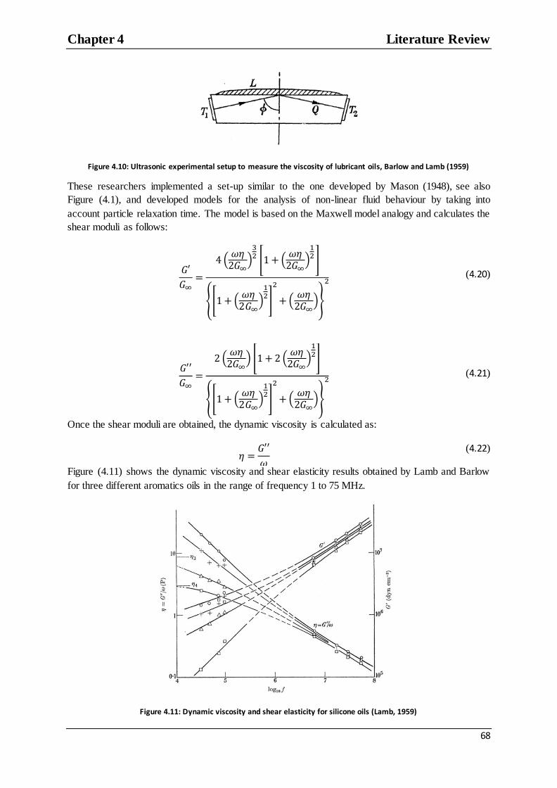
Chapter 4 Literature Review
68
Figure 4.10: Ultrasonic experimental setup to measure the viscosity of lubricant oils, Barlow and Lamb (1959)
These researchers implemented a set-up similar to the one developed by Mason (1948), see also
Figure (4.1), and developed models for the analysis of non-linear fluid behaviour by taking into
account particle relaxation time. The model is based on the Maxwell model analogy and calculates the
shear moduli as follows:
(𝜔
)
[ (
𝜔
)
]
{[ (𝜔
)
]
(𝜔
)}
(4.20)
(𝜔
) [ (𝜔
)
]
{[ (𝜔
)
]
(𝜔
)}
(4.21)
Once the shear moduli are obtained, the dynamic viscosity is calculated as:
𝜔
(4.22)
Figure (4.11) shows the dynamic viscosity and shear elasticity results obtained by Lamb and Barlow
for three different aromatics oils in the range of frequency 1 to 75 MHz.
Figure 4.11: Dynamic viscosity and shear elasticity for silicone oils (Lamb, 1959)
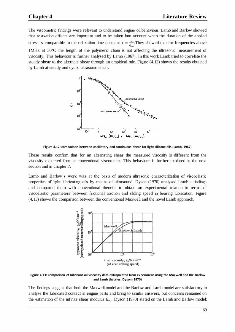
Chapter 4 Literature Review
69
The viscometric findings were relevant to understand engine oil behaviour. Lamb and Barlow showed
that relaxation effects are important and to be taken into account when the duration of the applied
stress is comparable to the relaxation time constant 𝜏
.They showed that for frequencies above
1MHz at 30°C the length of the polymeric chain is not affecting the ultrasonic measurement of
viscosity. This behaviour is further analysed by Lamb (1967). In this work Lamb tried to correlate the
steady shear to the alternate shear through an empirical rule. Figure (4.12) shows the results obtained
by Lamb at steady and cyclic ultrasonic shear.
Figure 4.12: comparison between oscillatory and continuous shear for light silicone oils (Lamb, 1967)
These results confirm that for an alternating shear the measured viscosity is different from the
viscosity expected from a conventional viscometer. This behaviour is further explored in the next
section and in chapter 7.
Lamb and Barlow‟s work was at the basis of modern ultrasonic characterization of viscoelastic
properties of light lubricating oils by means of ultrasound. Dyson (1970) analysed Lamb‟s findings
and compared them with conventional theories to obtain an experimental relation in terms of
viscoelastic parameters between frictional traction and sliding speed in bearing lubrication. Figure
(4.13) shows the comparison between the conventional Maxwell and the novel Lamb approach.
Figure 4.13: Comparison of lubricant oil viscosity data extrapolated from experiment using the Maxwell and the Barlow
and Lamb theories, Dyson (1970)
The findings suggest that both the Maxwell model and the Barlow and Lamb model are satisfactory to
analyse the lubricated contact in engine parts and bring to similar answers, but concerns remained on
the estimation of the infinite shear modulus . Dyson (1970) stated on the Lamb and Barlow model:

Chapter 4 Literature Review
70
“Some features remain unexplained, and there is need for more information, particularly on the
variation with pressure and temperature of the limiting shear modulus in oscillatory shear”.
More recently, Verdier et al. (1998) used the ultrasonic technique developed by Lamb and Barlow to
compare the evolution of light silicon oils shear moduli over the last decades to determine how the oil
market has been evolving throughout the XX century.
The work of Lamb and Barlow was certainly innovative, but the viscoelastic parameters of the oils,
such as the fluid complex shear modulus, were a function of parameters that are impossible to
measure accurately outside the laboratory environment. This is the case of the infinite shear modulus
that is the shear modulus obtained if an infinite stress is applied at the oil surface. This does not make
it possible to apply the Barlow technique in practical applications because the ultrasonic measurement
is not standalone.
4.7 Comparison of Ultrasonic Viscometers and Conventional Viscometers
All the previously mentioned authors claimed to measure the shear viscosity of fluids by the use of
vibrational techniques, but an important difference exists between vibrational techniques and steady
shear techniques (or the conventional viscometers). Cox and Merz (1958) were the first to study the
correlation between steady shear and vibrational shear. These researchers showed that the
mechanically induced shear rate in a conventional viscometer is the same as the shear rate induced at
the equivalent vibrational frequency in a rotational viscometer. This consideration is known as the
Cox-Merz rule:
𝜔 | (4.23)
At that time it was possible to prove this rule only in the shear rate range of s-1
and the
work conducted at low ultrasonic frequency, such as the Mason or the Woodward‟s one (1958), was
validated. Figure (4.14) shows the results obtained by Yu et al. (2004) in an attempt to validate this
rule.
Figure 4.14: comparison of the viscosity measured with conventional techniques (solid line) and oscillatory measurement (circles), Yu et al. (2004)
It is possible to see that the results at steady and oscillatory shear start deviating for shear rates above
s-1
. Following Cox and Merz, other more complex rules to correlate steady shear and vibrational
shear were made. It is the case of the Laun‟s rule (Laun, 1986):
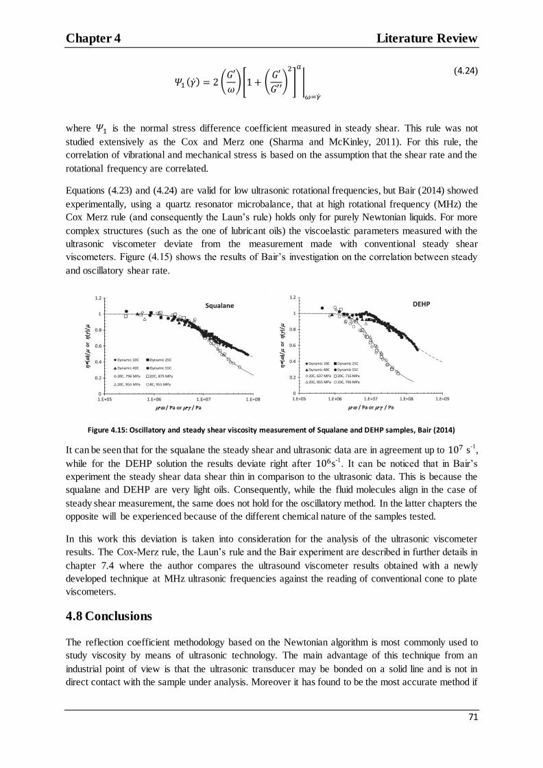
Chapter 4 Literature Review
71
(
𝜔)[ (
)
]
|
(4.24)
where is the normal stress difference coefficient measured in steady shear. This rule was not
studied extensively as the Cox and Merz one (Sharma and McKinley, 2011). For this rule, the
correlation of vibrational and mechanical stress is based on the assumption that the shear rate and the
rotational frequency are correlated.
Equations (4.23) and (4.24) are valid for low ultrasonic rotational frequencies, but Bair (2014) showed
experimentally, using a quartz resonator microbalance, that at high rotational frequency (MHz) the
Cox Merz rule (and consequently the Laun‟s rule) holds only for purely Newtonian liquids. For more
complex structures (such as the one of lubricant oils) the viscoelastic parameters measured with the
ultrasonic viscometer deviate from the measurement made with conventional steady shear
viscometers. Figure (4.15) shows the results of Bair‟s investigation on the correlation between steady
and oscillatory shear rate.
Figure 4.15: Oscillatory and steady shear viscosity measurement of Squalane and DEHP samples, Bair (2014)
It can be seen that for the squalane the steady shear and ultrasonic data are in agreement up to s-1
,
while for the DEHP solution the results deviate right after s-1
. It can be noticed that in Bair‟s
experiment the steady shear data shear thin in comparison to the ultrasonic data. This is because the
squalane and DEHP are very light oils. Consequently, while the fluid molecules align in the case of
steady shear measurement, the same does not hold for the oscillatory method. In the latter chapters the
opposite will be experienced because of the different chemical nature of the samples tested.
In this work this deviation is taken into consideration for the analysis of the ultrasonic viscometer
results. The Cox-Merz rule, the Laun‟s rule and the Bair experiment are described in further details in
chapter 7.4 where the author compares the ultrasound viscometer results obtained with a newly
developed technique at MHz ultrasonic frequencies against the reading of conventional cone to plate
viscometers.
4.8 Conclusions
The reflection coefficient methodology based on the Newtonian algorithm is most commonly used to
study viscosity by means of ultrasonic technology. The main advantage of this technique from an
industrial point of view is that the ultrasonic transducer may be bonded on a solid line and is not in
direct contact with the sample under analysis. Moreover it has found to be the most accurate method if

Chapter 4 Literature Review
72
a sensitive solid line is provided. Nevertheless the following limitations preclude the use of any of the
previous methods for in-situ viscosity measurement in engine components:
All the methods developed so far that can be applied in-situ, for instance the reflection
coefficient methodology, can measure only the viscosity of Newtonian oils.
The methods that allow measurements of Non-Newtonian viscosity are not stand-alone and so
cannot be used for in-situ applications.
The quartz resonators technique is not suitable for on-site fluid investigation because the
quartz cannot resist the temperature and pressures in the lubricated contact.
The attenuation and time of flight measurement technique cannot be applied in-situ at the
current state of the art because the method cannot be applied to the thin films that are
common in lubricated contacts.
The study of the ultrasonic viscometry literature brings the following important considerations that are
the foundation for the development of a non-invasive ultrasonic viscometer for applications in the
study of bearing lubrication:
The shear reflection coefficient technique is the most suitable method implemented because
the transducer is not submerged in the fluid and the lubricant layer thickness is not a
parameter that influences the measurement response. This is proven by the wide variety of
industrial applications for this technique.
A novel analytical model that takes into account lubricant viscoelasticity, but that is
implemented with measurable quantities has to be implemented.
A novel sensing technique has to be developed to allow the application of the reflectance
technique with materials of engineering interest for bearing applications (for instance steel
and not quartz or polymer).
The measurement made with the ultrasonic viscometer has to be compared with the steady
shear measurement for a fully understanding of the quantity that is measured.
The methods to measure viscosity using ultrasound are summarized in table 4.1. Appendix A reports a
table that summarizes the literature review of ultrasound viscosity methods to measure viscosity.

Chapter 4 Literature Review
73
Method Advantage Disadvantage Application Quartz resonator
Precise for Newtonian viscosity measurement.
Not good for in line lubricant characterization as the transducer has to be in contact with the liquid under analysis.
Characterization of fluids in laboratory environment.
Rod resonator Precise for Newtonian viscosity measurement, possibility to excite several modes (plane, surface, Rayleigh) inside the fluid sample under analysis.
Too many variables involved in the process compared to other techniques. Need for a calibrated line to guide the waves.
Characterization of fluids in laboratory environment.
Reflection coefficient (plane waves)
Relate the reflection coefficient to Newtonian and Non-Newtonian fluid properties.
Applicable in-situ for industrial application as the ultrasonic transducer may be mounted on a delay line.
Shear reflection coefficient allows for direct measurement of rheological parameters of interest (e.g. elastic shear modulus)
Measurements are sensitive to acoustic mismatch between delay line and fluid sample. As with all other techniques, acquisition is really sensitive to temperature variations.
In line clean up processes. Characterization of slurries. Characterization of resins in autoclave.
Attenuation coefficient
Based on reflection coefficient analysis.
Measurements are limited to fluid in a bulk
Characterization of slurries. Characterization of industrial wastes. Characterization of fluids in pipes.
Spectroscopy Wide range of frequency involved.
Precise to analyse Newtonian fluids.
A perfectly machined chamber has to be provided as spectroscopy techniques are based on speed of sound (time of flight) measurements.
Characterization of fluids in laboratory environment.
Table 4.1: Recap of methods to measure viscosity by means of ultrasonic technology

Chapter 5 A Novel Ultrasonic Model for Non-Newtonian Fluids
74
Chapter 5 A Novel Ultrasonic Model for
Non-Newtonian Fluids
A Novel Ultrasonic Model for
Non-Newtonian Fluids
Chapter 4 highlighted the necessity to develop a model that correlates the viscosity of Non-Newtonian
oils to the shear reflection coefficient. In this chapter the Maxwell model is derived and simplified to
obtain an analytical model that is function of the reflection coefficient only. The Maxwell model is
then compared with the Newtonian algorithms and its efficiency is tested through a sensitivity
analysis.
5.1 Introduction
The Newtonian solution of the wave equation (equation 4.9) and the Greenwood model (equation
(4.15)) can be easily implemented with a common ultrasonic reflectance set-up (see chapter 6) for
non-invasive analysis, but they do not allow the precise measurement of complex polymeric oils. On
the other hand, the Non-Newtonian Maxwell models introduced by Lamb (1967) and Barlow (1959)
are very complex to be practically implemented. It is impossible to use the ultrasonic method with
these complex algorithms due to the presence of terms in the viscoelastic model such as the viscosity
at infinite strain. This limits the applicability in-situ of these techniques. In this chapter the Maxwell
fluid analogy (Maxwell, 1860) is further simplified to obtain a direct correlation between the
experimentally measured reflection coefficient and the viscosity. The aim is to obtain a stand-alone
technique that allows viscosity measurement by analysis of the ultrasonic reflection only.
Several viscoelastic models exist. Some examples are the Wiechert model (1893) and the Boltzman
integral solution (Markovitz, 1977). These models are considered more precise than the Maxwell
model because they describe more completely complex fluids. For example, the Wiechert model
considers multiple relaxation times, while the Boltzman overcome the simplicity of the viscoelastic
mechanical analogy through a complex integral solution. In this work, the Maxwell model is chosen
for its simplicity and because it takes into account the main viscoelastic parameters and the main fluid
relaxation time, thus approximating with sufficient precision the lubricant oil behaviour. For the same
reasons, this model was extensively used to study the rheological behaviour of lubricant oils. Hutton
(1967) validated the findings of Barlow and Lamb by applying their Maxwell model to study the
relaxation behaviour of a selection of engine oils. Johnson and Teevarwerk (1977) used a non-linear
isothermal Maxwell model to analyse the traction forces at the contact interface between oil and disc
on a two-disc machine. Bair and Wiener (1980) applied another modification to the Maxwell model to
predict oil behaviour in elasto-hydrodynamic (EHD) lubrication regime.
5.2 The Maxwell Fluid Model
To build the models described in equations (4.9) and (4.15) the assumption of Newtonian response of
the fluid to shear stress excitation was made and viscosity was calculated by rearranging equation
(3.34) as function of the reflection coefficient. Most lubricants operating in mixed or EHD lubrication
conditions are non-Newtonian and relaxation effects are not negligible, for example in operating
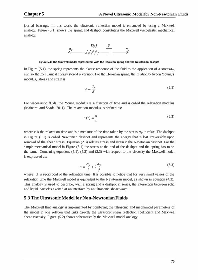
Chapter 5 A Novel Ultrasonic Model for Non-Newtonian Fluids
75
journal bearings. In this work, the ultrasonic reflection model is enhanced by using a Maxwell
analogy. Figure (5.1) shows the spring and dashpot constituting the Maxwell viscoelastic mechanical
analogy.
Figure 5.1: The Maxwell model represented with the Hookean spring and the Newtonian dashpot
In Figure (5.1), the spring represents the elastic response of the fluid to the application of a stress ,
and so the mechanical energy stored reversibly. For the Hookean spring, the relation between Young‟s
modulus, stress and strain is:
𝜀
(5.1)
For viscoelastic fluids, the Young modulus is a function of time and is called the relaxation modulus
(Mainardi and Spada, 2011). The relaxation modulus is defined as:
𝜏
(5.2)
where 𝜏 is the relaxation time and is a measure of the time taken by the stress to relax. The dashpot
in Figure (5.1) is called Newtonian dashpot and represents the energy that is lost irreversibly upon
removal of the shear stress. Equation (2.3) relates stress and strain in the Newtonian dashpot. For the
simple mechanical model in Figure (5.1) the stress at the end of the dashpot and the spring has to be
the same. Combining equations (5.1), (5.2) and (2.3) with respect to the viscosity the Maxwell model
is expressed as:
𝜆
(5.3)
where 𝜆 is reciprocal of the relaxation time. It is possible to notice that for very small values of the
relaxation time the Maxwell model is equivalent to the Newtonian model, as shown in equation (4.3).
This analogy is used to describe, with a spring and a dashpot in series, the interaction between solid
and liquid particles excited at an interface by an ultrasonic shear wave.
5.3 The Ultrasonic Model for Non-Newtonian Fluids
The Maxwell fluid analogy is implemented by combining the ultrasonic and mechanical parameters of
the model in one relation that links directly the ultrasonic shear reflection coefficient and Maxwell
shear viscosity. Figure (5.2) shows schematically the Maxwell model analogy.

Chapter 5 A Novel Ultrasonic Model for Non-Newtonian Fluids
76
Figure 5.2 Maxwell analogy to describe contact interface particle interaction due to applied shear ultrasonic stress
The damper element models the relaxation effects of a viscoelastic system as ultrasonic shear occurs
at the solid-liquid boundary. The interaction between a solid particle and the liquid particle ,
both subjected to ultrasonic displacements v and v , is described by a mechanical analogy. As it was
stated in section 5.2, the total stress and strain in the system are given by:
and (5.4)
where is the total stress, the total strain, the subscript s refers to the spring element while the
subscript d to the dashpot. From Hooke‟s law and from the dashpot theory:
and
(5.5)
Differentiating equations (5.4) and substituting in equations (5.5) gives:
(5.6)
where k (or in Barlow and Lamb (1959)) is the stiffness of the spring defined as
, and 𝜏 is the
relaxation time. In the case of sinusoidal varying stress, the stress and strain are:
and (5.7)
Substituting equations (5.7) in equation (5.6) gives:
𝜔 ( 𝜔
𝜏)
(5.8)
Now by substituting equation (5.8) into the definition of shear modulus stated in equation (3.36):
𝜔𝜏
𝜔𝜏 (
𝜔 𝜏
𝜔 𝜏 𝜔𝜏
𝜔 𝜏 )
(5.9)
Substituting the stiffness
into equation (5.9) gives:
(𝜔 𝜏
𝜔 𝜏 𝜔
𝜔 𝜏 )
(5.10)
Separating the real and imaginary part gives:

Chapter 5 A Novel Ultrasonic Model for Non-Newtonian Fluids
77
{
𝜔 𝜏
𝜔 𝜏
𝜔
𝜔 𝜏
(5.11)
The system of equations (5.11) is a system of two equations with two unknowns, and 𝜏. Solving the
two equations simultaneously leads to the solution for the viscosity in case the relaxation effects are
taken into account. It is possible to compare the Maxwell model expressed in equations (5.11) with the
Newtonian solutions reported in chapter 4 as follows. Expressing the second equation of (5.11) with
respect to gives:
𝜔 𝜏
𝜔
(5.12)
The storage and loss moduli and are related to the ultrasonic reflection coefficient by equation
(3.41) and can be measured experimentally. They are therefore known parameters. Combining these
equations with (5.10) leads to:
( (
)) 𝜔 𝜏
𝜔
(5.13)
Substituting the definition of shear acoustic impedance, equation (3.41), into equation (5.13) it is
possible to directly correlate the reflection coefficient to the shear viscosity:
( 𝜃
𝜃 ) 𝜔 𝜏
𝜔
(5.14)
where 𝜏 is a known parameter that can be obtained from the first equation of (5.11). It can be noticed
that equation (5.14) is equivalent to equation (4.9) except for the term 𝜔 𝜏 . When 𝜔 𝜏 then
equation (5.12) reduces to the Newtonian solution of the wave equation (4.9).
5.4 Comparison of Models
The ultrasonic models (the Newtonian (4.9), the Greenwood (4.15) and the Maxwell (5.14)) relate the
fluid shear modulus to the viscosity through the shear reflection coefficient. The propagation of an
ultrasonic wave at a solid-oil boundary can be described with an electrical analogy. This kind of
analogy is very helpful to explain the differences between the Newtonian and the Non-Newtonian
models. When an ultrasonic wave travels through a solid, stress and strain are in phase and the shear
modulus value is a real number, consequently the solid layer acts like a resistance with respect to the
ultrasonic wave motion because the vibrational energy is partly dissipated in the propagation. When
an ultrasonic wave is incident to a Newtonian fluid boundary, stress and strain are out of phase by 90
degrees. This is equivalent to a pure capacitance element, as stated in section 5.1. Figure (5.3 a) shows
the propagation of a shear wave at a solid-Newtonian fluid interface as an electrical analogy with a
resistance (solid) and a capacitance (fluid) in series. This electric circuit applies to the ultrasonic

Chapter 5 A Novel Ultrasonic Model for Non-Newtonian Fluids
78
Newtonian models. The Maxwell model differs because it takes into account of the viscoelastic
behaviour of real lubricants. For these fluids the stress and strain are out of phase of a quantity that is
between 0 and 90 degrees. Figure (5.3 b) shows the electrical circuit that represents this situation
using a variable gain resistance (equivalent to ) and a capacitance in series.
Figure 5.3 Electrical analogy to describe the incident ultrasonic wave to (a) Newtonian and (b) Viscoelastic fluids
In the Maxwell model, the value of the variable gain resistance is correlated to the relaxation time.
When the relaxation time increases, the Non-Newtonian grade of the oil is accentuated and the circuit
in Figure (5.3 b) becomes totally resistive. Figure (5.4) shows the amplitude of G versus frequency as
the relaxation time of the lubricant is changed, from equations (4.9) and (5.14).
Figure 5.4: Comparison shear storage modulus (a) and loss modulus (b) from Newtonian and Maxwell models as the relaxation time changes
a) b)

Chapter 5 A Novel Ultrasonic Model for Non-Newtonian Fluids
79
For low values of the relaxation time (so for𝜔 𝜏 ), the Newtonian and the Maxwell models are
identical. In the electric circuit analogy this corresponds to a situation where the variable gain
resistance in Figure (5.3 b) is negligible. For high values of the relaxation time the value is of the
same order as and the Newtonian model fails in describing the real oil behaviour. Figure (5.5)
shows the three different models for equations (4.9), (4.15) and (5.14) are compared for different
liquid relaxation times. For low relaxation times the three algorithms give a similar response, while for
higher values of relaxation time only the Maxwell model is sensitive to the fluid structure changes. In
all cases, for the viscosities considered, the reflection coefficient is close to one. This is a serious
limitation in the practical implementation of these methods on a lubricant viscometer, as described in
chapter 6.
Figure 5.5: Application of Newtonian and Maxwell model for different relaxation times at an aluminium -liquid boundary
Table (5.1) recaps and compares the three reflectance models.
Model Mechanical Model
Ultrasound Model = f(R) Mechanical Analogy
Newtonian
𝜔* 𝜃
𝜃+
Greenwood
( (
𝜔)
(
))
Maxwell
𝜆
( 𝜃
𝜃 )
𝜔 𝜏
𝜔
Table 5.1: Summary of the ultrasonic models to predict viscosity
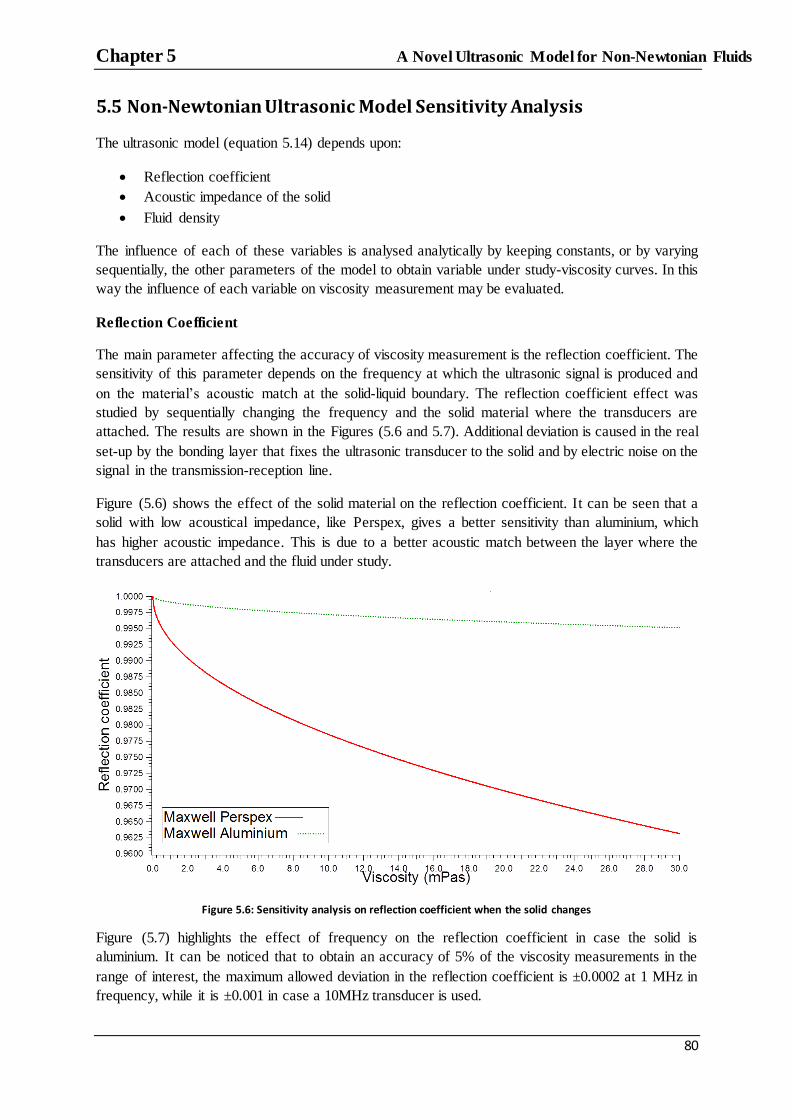
Chapter 5 A Novel Ultrasonic Model for Non-Newtonian Fluids
80
5.5 Non-Newtonian Ultrasonic Model Sensitivity Analysis
The ultrasonic model (equation 5.14) depends upon:
Reflection coefficient
Acoustic impedance of the solid
Fluid density
The influence of each of these variables is analysed analytically by keeping constants, or by varying
sequentially, the other parameters of the model to obtain variable under study-viscosity curves. In this
way the influence of each variable on viscosity measurement may be evaluated.
Reflection Coefficient
The main parameter affecting the accuracy of viscosity measurement is the reflection coefficient. The
sensitivity of this parameter depends on the frequency at which the ultrasonic signal is produced and
on the material‟s acoustic match at the solid-liquid boundary. The reflection coefficient effect was
studied by sequentially changing the frequency and the solid material where the transducers are
attached. The results are shown in the Figures (5.6 and 5.7). Additional deviation is caused in the real
set-up by the bonding layer that fixes the ultrasonic transducer to the solid and by electric noise on the
signal in the transmission-reception line.
Figure (5.6) shows the effect of the solid material on the reflection coefficient. It can be seen that a
solid with low acoustical impedance, like Perspex, gives a better sensitivity than aluminium, which
has higher acoustic impedance. This is due to a better acoustic match between the layer where the
transducers are attached and the fluid under study.
Figure 5.6: Sensitivity analysis on reflection coefficient when the solid changes
Figure (5.7) highlights the effect of frequency on the reflection coefficient in case the solid is
aluminium. It can be noticed that to obtain an accuracy of 5% of the viscosity measurements in the
range of interest, the maximum allowed deviation in the reflection coefficient is ±0.0002 at 1 MHz in
frequency, while it is ±0.001 in case a 10MHz transducer is used.
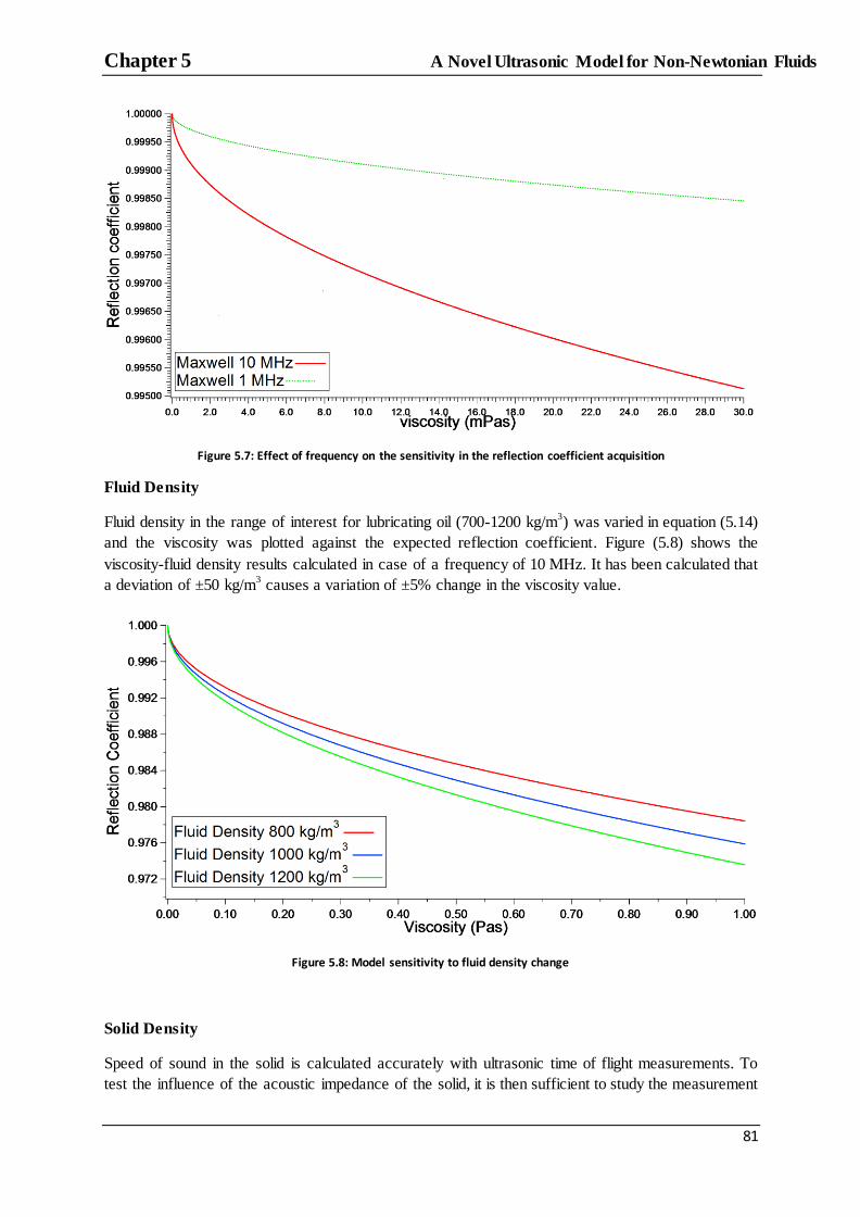
Chapter 5 A Novel Ultrasonic Model for Non-Newtonian Fluids
81
Figure 5.7: Effect of frequency on the sensitivity in the reflection coefficient acquisition
Fluid Density
Fluid density in the range of interest for lubricating oil (700-1200 kg/m3) was varied in equation (5.14)
and the viscosity was plotted against the expected reflection coefficient. Figure (5.8) shows the
viscosity-fluid density results calculated in case of a frequency of 10 MHz. It has been calculated that
a deviation of ±50 kg/m3 causes a variation of ±5% change in the viscosity value.
Figure 5.8: Model sensitivity to fluid density change
Solid Density
Speed of sound in the solid is calculated accurately with ultrasonic time of flight measurements. To
test the influence of the acoustic impedance of the solid, it is then sufficient to study the measurement
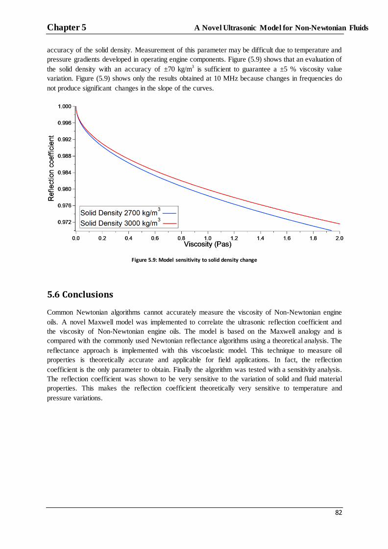
Chapter 5 A Novel Ultrasonic Model for Non-Newtonian Fluids
82
accuracy of the solid density. Measurement of this parameter may be difficult due to temperature and
pressure gradients developed in operating engine components. Figure (5.9) shows that an evaluation of
the solid density with an accuracy of ±70 kg/m3 is sufficient to guarantee a ±5 % viscosity value
variation. Figure (5.9) shows only the results obtained at 10 MHz because changes in frequencies do
not produce significant changes in the slope of the curves.
Figure 5.9: Model sensitivity to solid density change
5.6 Conclusions
Common Newtonian algorithms cannot accurately measure the viscosity of Non-Newtonian engine
oils. A novel Maxwell model was implemented to correlate the ultrasonic reflection coefficient and
the viscosity of Non-Newtonian engine oils. The model is based on the Maxwell analogy and is
compared with the commonly used Newtonian reflectance algorithms using a theoretical analysis. The
reflectance approach is implemented with this viscoelastic model. This technique to measure oil
properties is theoretically accurate and applicable for field applications. In fact, the reflection
coefficient is the only parameter to obtain. Finally the algorithm was tested with a sensitivity analysis.
The reflection coefficient was shown to be very sensitive to the variation of solid and fluid material
properties. This makes the reflection coefficient theoretically very sensitive to temperature and
pressure variations.

Chapter 6 Viscosity Measurement at an Aluminium-Oil Boundary
83
Chapter 6 Viscosity Measurement at
an Aluminium-Oil Boundary
Viscosity Measurements at an Aluminium-
Oil Boundary This Chapter describes the ultrasonic experimental apparatus and its application to measure the
viscosity at an aluminium-oil boundary. The conventional reflectance set-up is made of a pair of
ultrasonic transducers that are bonded on the top of an aluminium block in contact with a thin layer of
lubricant oil. The reflection coefficient is acquired when the oil is heated up and the viscosity is
calculated using the equations (4.9, 4.15 and 5.14). Finally, the results are compared with the reading
from a conventional cone-on-plate viscometer.
6.1 Ultrasonic Apparatus
The conventional experimental ultrasonic apparatus is shown schematically in Figure (6.1). The
piezoelectric transducers are glued to the test piece using a strain gauge adhesive. One transducer
acted as a pulser and the other as a receiver. This set-up is commonly known as pulse-echo. A
waveform function generator (TTI TG5011) produces a burst pulse excitation that is sent to the
transmitting ultrasonic transducer (pulser) producing an ultrasonic wave. The ultrasonic pulse from
the first transducer propagates through the solid until is incident to a boundary where part of the wave
is reflected. The reflected wave from the interface is received by the second transducer (receiver). The
reflected signal is recorded on an oscilloscope (Lecroy LT342), continuously analysed, averaged and
stored in real time using an acquisition interface written in Labview™.
Figure 6.1 Experimental Apparatus
The arbitrary waveform generator and the oscilloscope represent the pulsing/receiving
instrumentation. The main characteristics of this system are: voltage, frequency, repetition rate,
sampling rate.

Chapter 6 Viscosity Measurement at an Aluminium-Oil Boundary
84
The voltage is the amplitude of the excitation pulse. Common values range from 1 to 10 V.
This value can be controlled or increased by adding an amplification system in the
measurement line.
The frequency is the inverse of the period of the excitation pulse and is set to match the
desired pulsing frequency of the transducer.
The repetition rate is the rate at which the signals are sent to the ultrasonic transducer from
the waveform generator. It is a critical factor only in dynamic tests where the transducer
should produce and receive a high number of ultrasonic signals.
The sampling rate is a characteristic of the oscilloscope and determines the capacity of a
system to discretize a continuous signal, such as a waveform, in a discrete number of points.
The sampling rate of the LeCroy oscilloscope is 500 MHz. This tool allows to average up to
1000 signals to filter out any random electric noise before transferring data to the computer.
6.1.1 The Transducers
Figure (6.2) shows the ultrasonic transducers bonded on the aluminium surface. The transducer
chosen for this experiment are a pair of 10 MHz wraparound chrome-gold coated PZ-5A bare
piezoelectric element. PZ-5A is a grade of the lithium metanobiate PZTs and is normally used for
industrial application. The Curie temperature (the temperature at which the crystal loses the
piezoelectric properties) is 250 °C making it ideal for laboratory temperature applications that involve
a temperature change. The operating frequency is 10 MHz. This is chosen to have a penetration depth
less than 1μm so that the ultrasound wave is reflected from the solid-oil boundary and is not
transmitted to the bottom of the fluid layer.
Figure 6.2: The ultrasonic transducers
6.1.2 The Cables
The cables used to connect the transducer to the pulsing/receiving equipment are coaxial cables with
external diameter of 1.2 mm and signal attenuation of 2.3 dB/m at 1 GHz.

Chapter 6 Viscosity Measurement at an Aluminium-Oil Boundary
85
Figure 6.3: Coaxial cable structure, picture property of Nexans
This type of cable is chosen for the low signal attenuation capabilities and for its flexibility. This is an
important requirement because the transducers, due to their thinness, cannot be stressed to avoid
breakage, or to cause damage to the coated electrode. In this work the shield is used as connection for
the ground providing a resistance of 50 Ohm, while the conductor is connected to the transducer.
Figure (6.4) shows the soldered connection between the coaxial cable and the ultrasonic transducer.
Figure 6.4: Connection of the coaxial cable to the ultrasonic transducer
6.1.3 Thermocouple Calibration
The thermocouples were calibrated with respect to a RTD system. This is the best thermocouple
system available off the shelf and guarantees an accuracy of ±0.2°C. Unfortunately, the RTD probe is
very large and it cannot be used to acquire temperature from the thin layer within the set-up proposed
in Figure (6.1). On the other hand, k-type thermocouples are ideal because of the very small active
area (1mm length) and the small radius of the probe (0.8 mm), but their nominal accuracy is of
±0.5°C. Viscosity is very sensitive to temperature changes and the system used to measure the
temperature had to provide the maximum precision possible. The calibration of the k-type
thermocouple was then needed to make sure that the accuracy of temperature measurement was
within the RTD precision. To do so the RTD system and the k-type thermocouples were heated up in
the oven. The experiment was repeated twice and both in heating and cooling down. Figure (6.5)
shows the RTD reading against the k-type thermocouple reading.

Chapter 6 Viscosity Measurement at an Aluminium-Oil Boundary
86
Figure 6.5: K-type thermocouple calibration curves
It is possible to notice in Figure (6.5) that the reading from the RTD and the k type thermocouples
were very close. Also, between heating and cooling, no hysteresis is created and this is a confirmation
that the k-type thermocouple represents the ideal tool to perform the temperature measurement in this
experiment.
6.1.4 Test Lubricants
The samples tested were six different Cannon viscosity standard calibrated lubricants (information
about the test lubricants viscosities is reported in Table 6.1). The Cannon™ standard viscosity oils
tested were Newtonian mineral hydrocarbon base oils tested following the NIST (National Institute of
Standards and Technology) standards. The use of these oils was justified not only by their Newtonian
behaviour, but also by the amount of information supplied on these oils thus making it the right
reference for the calibration of a new sensing and measurement system.
Mineral oil @20°C (mPas) @40°C (mPas) @50°C (mPas) S20 37.32 15.27 10.65
S60 139.1 53.83 34.69 S200 587.4 177.5 155.8
N350 1114 270.3 151.1
S600 2008 446.2 240.4 S2000 9256 1662 808.2
Table 6.1 Cannon viscosity standard mineral oils tested
6.1.5 Experimental Protocol
Figure (6.6) shows the experimental apparatus used in the reflectance test. Two flat aluminium plates
were used to trap a thin layer of liquid; oil films in the range 20-100 um were generated. The film
thickness was known by interleaving at the sides of the aluminium plates two thin metal strips of
known thicknesses. Aluminium was chosen to simulate the engine materials in contraposition to the
plastic substrates that are normally used in laboratory experiments. On the upper plate, two
piezoelectric transducers (PZT) were bonded, as described in section 6.1.1. The bottom solid plate had
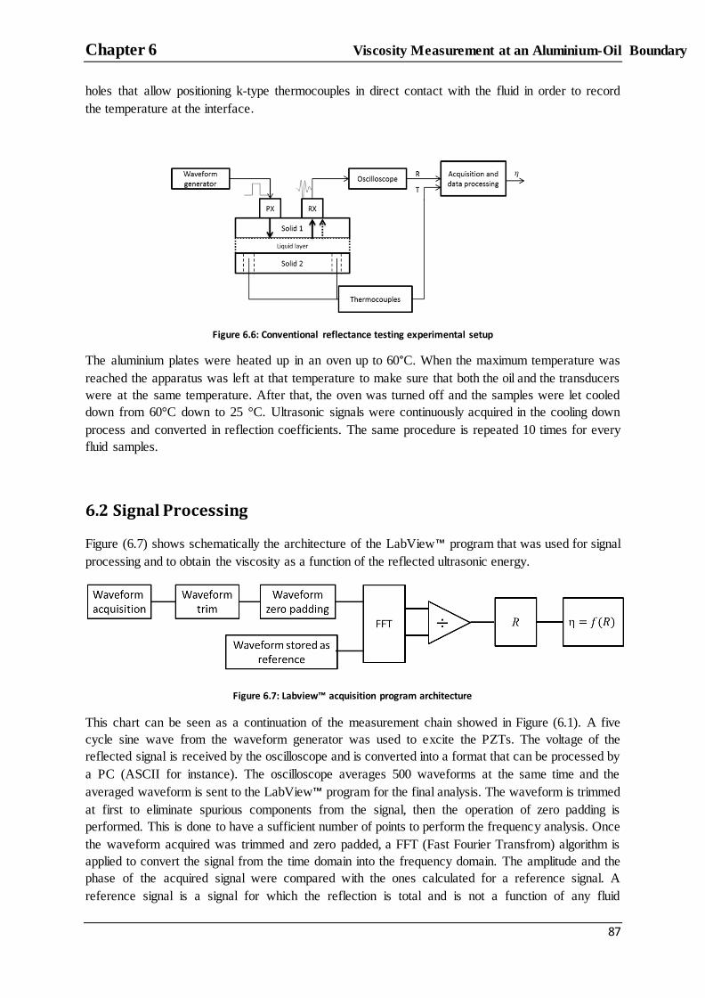
Chapter 6 Viscosity Measurement at an Aluminium-Oil Boundary
87
holes that allow positioning k-type thermocouples in direct contact with the fluid in order to record
the temperature at the interface.
Figure 6.6: Conventional reflectance testing experimental setup
The aluminium plates were heated up in an oven up to 60°C. When the maximum temperature was
reached the apparatus was left at that temperature to make sure that both the oil and the transducers
were at the same temperature. After that, the oven was turned off and the samples were let cooled
down from 60°C down to 25 °C. Ultrasonic signals were continuously acquired in the cooling down
process and converted in reflection coefficients. The same procedure is repeated 10 times for every
fluid samples.
6.2 Signal Processing
Figure (6.7) shows schematically the architecture of the LabView™ program that was used for signal
processing and to obtain the viscosity as a function of the reflected ultrasonic energy.
Figure 6.7: Labview™ acquisition program architecture
This chart can be seen as a continuation of the measurement chain showed in Figure (6.1). A five
cycle sine wave from the waveform generator was used to excite the PZTs. The voltage of the
reflected signal is received by the oscilloscope and is converted into a format that can be processed by
a PC (ASCII for instance). The oscilloscope averages 500 waveforms at the same time and the
averaged waveform is sent to the LabView™ program for the final analysis. The waveform is trimmed
at first to eliminate spurious components from the signal, then the operation of zero padding is
performed. This is done to have a sufficient number of points to perform the frequency analysis. Once
the waveform acquired was trimmed and zero padded, a FFT (Fast Fourier Transfrom) algorithm is
applied to convert the signal from the time domain into the frequency domain. The amplitude and the
phase of the acquired signal were compared with the ones calculated for a reference signal. A
reference signal is a signal for which the reflection is total and is not a function of any fluid

Chapter 6 Viscosity Measurement at an Aluminium-Oil Boundary
88
properties, thus being the ideal comparison term with the signal attenuated from the fluid. The
reference signal was obtained by removing the fluid sample from the upper aluminium block to
acquire a waveform at a solid-air boundary. The signal acquired from the solid-liquid interface was
called measurement signal and the amplitude of this signal, , was attenuated compared to the
reference amplitude because part of the energy was dissipated at the fluid contact interface due to the
fluid viscosity. The reflection coefficient was obtained by dividing the measurement amplitude by the
reference amplitude as:
Similarly the phase is obtained as:
(6.1)
𝜃 𝜃 𝜃
(6.2)
where is the measurement amplitude, calculated with the FFT at the centre frequency of 10 MHz,
of the reflected signal from the solid liquid interface, is the amplitude of the reflected signal from
the solid-air interface (reference measurement) as shown in Figure (6.8), 𝜃 the phase of the reflected
signal from the solid liquid interface, and 𝜃 is the phase of the reflected signal from the solid-air
interface. The reflection coefficient was calculated this way because the solid-air interface constitutes
a very good reference, since almost 100% of the ultrasonic energy was reflected from air. The
reflection from a fluid layer was, on the other hand, affected by some energy being transmitted and
dissipated in the fluid. The comparison of the two reflections was then a good indicator of the effect
of the fluid on the ultrasound response and the ratio of the amplitude reflected from the liquid and the
air constitute the so called reflection coefficient.
The phase is very sensitive to temperature changes (±0.1 °C leads to ± 10 degrees of error) and the
following relation defining the phase is obtained by manipulating equation (3.40) (Franco et al.,
2010):
𝜃
(6.3)
The signals acquired in the time domain were then converted to the frequency domain using a FFT
(Fast Fourier transform), see Figure (6.8b). Once the FFT was performed the reflection coefficient
was obtained from equation (6.1) by dividing the measurement FFT by the reference FFT at the
desired frequency. In the application of the three methodologies only the reflection coefficient
component at the centre resonance frequency of the shear crystal (10 MHz) was considered. The
reflection coefficient value obtained with this procedure was then used in equations (4.9), (4.15) and
(5.14) to obtain oil sample viscosity.
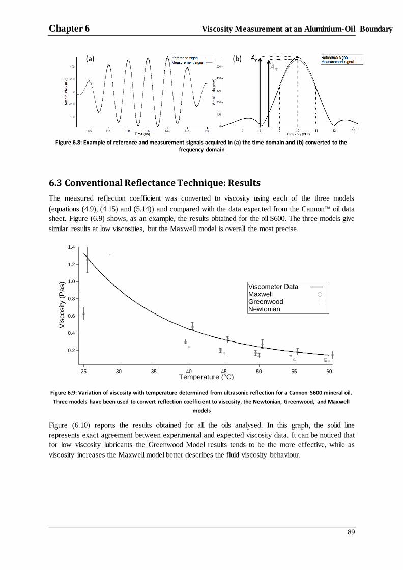
Chapter 6 Viscosity Measurement at an Aluminium-Oil Boundary
89
Figure 6.8: Example of reference and measurement signals acquired in (a) the time domain and (b) converted to the frequency domain
6.3 Conventional Reflectance Technique: Results
The measured reflection coefficient was converted to viscosity using each of the three models
(equations (4.9), (4.15) and (5.14)) and compared with the data expected from the Cannon™ oil data
sheet. Figure (6.9) shows, as an example, the results obtained for the oil S600. The three models give
similar results at low viscosities, but the Maxwell model is overall the most precise.
Figure 6.9: Variation of viscosity with temperature determined from ultrasonic reflection for a Cannon S600 mineral oil.
Three models have been used to convert reflection coefficient to viscosity, the Newtonian, Greenwood, and Maxwell
models
Figure (6.10) reports the results obtained for all the oils analysed. In this graph, the solid line
represents exact agreement between experimental and expected viscosity data. It can be noticed that
for low viscosity lubricants the Greenwood Model results tends to be the more effective, while as
viscosity increases the Maxwell model better describes the fluid viscosity behaviour.
1.4
1.2
1.0
0.8
0.6
0.4
0.2
Vis
cosity (
Pa
s)
6055504540353025
Temperature (°C)
Viscometer Data Maxwell Greenwood Newtonian
(a) (b)

Chapter 6 Viscosity Measurement at an Aluminium-Oil Boundary
90
Figure 6.10: Comparison of measured viscosity against expected data sheet values for all fluid samples tested
Using the data of Figure (6.10), Figure (6.11) shows the error between the ultrasonic measured
viscosity and the data sheet value. Three distinct regions can be identified.
Figure 6.11: Error associated with each reflection model. Three regions are shown: 1) R tends to 1 and all models are
subject to scatter, (2) the optimum region for the Greenwood model, (3) the optimum region for the Maxwell model
Region 1 is characterized by a high error for all the models, equations (4.9), (4.15) and (5.14). This is
because for a metal-liquid interface and for lubricant with low viscosity, the reflection coefficient
modulus is very close to the unity. As a consequence, any noise in the measurement line has a
significant effect on the result. For example, a variation of ±1% in the reflection coefficient can lead
to a deviation of ±25mPas from the theoretical viscosity value. So for the low viscosity oil S20, the
viscosity is 10 mPas at 55 °C while the measured value varies with an error of 20% to 100 %
depending on the model used. The reason the reflection coefficient is very close to one at metal-oil
interfaces is further analysed in section 6.4.
In the second region, the Greenwood Model gives the minimum error. In this region, most of the
results give an average error of about the 10% and the mineral oils analysed can be considered as
perfectly Newtonian. These results are in line with the accuracy obtained by other researchers (Sheen
et al., 1994).

Chapter 6 Viscosity Measurement at an Aluminium-Oil Boundary
91
In region 3, the Maxwell model gives the best precision. At around 0.15 Pas the Maxwell model
converges to the minimum error (less than 12%) while the accuracy of the Newtonian models diverge
quickly. This is because the Non-Newtonian behaviour is accentuated as the viscosity increases.
6.4 Conventional Reflectance Technique: Acoustic Mismatch
The viscosity results obtained from the application of the ultrasonic reflectance technique are affected
by a high error. This is accentuated for fluids with viscosity less than 10 mPas. This limits the
applicability of the reflectance technique to direct applications in engines because common values of
lubricant viscosity in operating engine components range from 5 to 20 mPas. The high measurement
error is due to the acoustic mismatch that occurs between solid and oil. Inspection of the reflection
coefficient equation (3.14) shows that when the acoustic impedance of the solid is much higher than
the acoustic impedance of the liquid the reflection coefficient tends to one. This is especially true for
metal-oil interfaces where the solid acoustic impedance can be one or two order of magnitude higher
than the modulus of the fluid shear acoustic impedance. In this situation, more than 99% of the
acoustic energy is reflected from the solid-liquid boundary. As a result the common reflectance
technique is highly insensitive to the oil properties, as the value of the reflection coefficient is very
close to the expected value for a solid-air interface. Since most engine components and bearings are
metallic, this practically precludes such a measurement method for in-situ and real time evaluation.
Table (6.2) lists the reflection coefficient acquired for the oils analysed in this section together with
the standard deviation. It is possible to notice that an error of ±1% in the acquisition of the reflection
coefficient does not allow discriminating among different fluids and consequently to obtain viscosity
measurements within an acceptable accuracy (± 5% difference in comparison to conventional
viscometers).
Sample Average reflection coefficient (thin layer)
Standard deviation
S20 0.9978 0.013
S60 0.9946 0.018
S200 0.9871 0.015 Table 6.2: Cannon viscosity standard mineral oils tested
At the current state of the art it is not possible to obtain reflection coefficient measurement with a
better accuracy of ±0.5% because of unavoidable noises and interferences created by the electrical
instrumentation. It then becomes clear that because of this inaccuracy a new technique is necessary to
allow viscosity measurement in engine.
6.5 Conclusions
The conventional reflectance technique was identified as the ideal method to measure viscosity in the
lubricated contacts in engines because the transducers can be miniaturized to fit the bearing geometry.
The reflectance technique was applied with the conventional setup to an aluminium-oil interface. The
experiment highlighted the effect of the greatest limitations of this method: the acoustic mismatch
between the solid and the liquid. When the transducers are bonded on a solid material with high
acoustic impedance, almost all of the ultrasonic energy is reflected and the measurement sensitivity is
very low in case of oils with viscosity of less than 0.02 Pas. The Maxwell model resulted to be the
Chapter 6 Viscosity Measurement at an Aluminium-Oil Boundary
92
most accurate system to predict viscosity when the liquid viscosity is higher than 0.3 Pas. This is the
case of engine oils under high load (for example the oil in a CVT transmission) or operating at low
temperatures, but it is not the case of journal bearings. The next sections present a novel method that
is developed to increase the measurement sensitivity for low viscosity oils.

Chapter 7 The Matching Layer Method
93
Chapter 7 The Matching Layer Method
The Matching Layer Method
This chapter presents the methodology used to overcome the limitations of the conventional
reflectance methodology. The ultrasound sensitivity to fluid viscosity is increased by interleaving a
layer of material between the solid and the oil. This layer matches the acoustic impedance of the solid
with the impedance of the oil and is called the matching layer. In this chapter the use of a matching
layer developed by the author is analysed analytically and then tested to measure the viscosity of oil
samples in a range of shear rates, temperatures and pressures. The method is able to precisely measure
the viscosity of Newtonian oils and to identify the Non-Newtonian nature of polymer lubricants.
7.1 Origins of the Matching Layer Methodology
The experimental viscosity results in chapter (6) showed that it is not possible to apply the
conventional ultrasonic reflectance technique with the materials commonly encountered in engines.
The difference in acoustic properties between the solid and oil in engine parts is such that all the
sound energy is reflected from the contact interface. This makes an accurate viscosity measurement
impossible. To overcome this limitation, a quarter wavelength matching layer is used to increase the
acoustic response by bonding it on the solid surface on the direction of the ultrasound wave path
propagation, as shown in Figure (7.1). In this picture it is schematically shown a comparison between
the common reflectance technique, Figures (7.1a and b), and the alternative matching layer method,
Figure (7.1c).
Figure 7.1: a) Shear ultrasound transmission and reflection from a solid-liquid boundary, (b) Shear ultrasound
transmission and reflection from a solid-liquid-solid system, (c) Shear ultrasound transmission and reflection from a solid-matching layer-liquid system
The quarter wavelength matching layer method is widely used to overcome impedance mismatch in
many electrical application. For example, the losses at the connections in long electric lines have to be
maintained as low as possible, and the materials that form the connection are interleaved with a
suitable material to match the different load at the terminations.
This method is also used in the production of ultrasonic immersion transducers or non-contact air
coupled probes. In this case, a layer with quarter wavelength thickness is bonded to the transducer and
is used to acoustically couple the piezoelectric element to water or air (Alvarez-Arenas, 2004). The
researchers that first applied this technique (Desiletes et al., 1978) treated the acoustic mismatch
between the ultrasonic transducer and the water with an electrical approach and compared the pzt-

Chapter 7 The Matching Layer Method
94
water system to an electrical circuit where the abrupt change in acoustic load acts as a short circuit, as
shown in Figure (7.2a).
Figure 7.2: Electrical analogy between system with and without matching layer
In Figure (7.2) are respectively the solid, liquid and matching layer acoustic impedance.
Figure (7.2a) represents a short circuit when and the short circuit is solved as shown in Figure
(7.2b) by the insertion of an appropriate acoustic load in between the previous two. This electrical
analogy has been the foundation of the matching layer methodology since the 50s (Mason, 1948 and
Collin, 1955). At that time the knowledge of the mechanics and physics of propagation of ultrasonic
waves in materials was very limited. The lack of experimental data and the high price of the ultrasonic
instrumentation brought the researchers to use the electrical analogy to study the acoustic mismatch
between different materials. Since then, different approaches to the problem have been presented,
ranging from the use of quarter wavelength, one-eighth of wavelength or multiple matching layers.
This technique found large use in industry for ultrasonic method employing longitudinal waves (for
example Haller, 1992), but surprisingly the literature is very poor in the application of this method to
shear wave-based techniques. In fact, no work currently exists in academia that applies the matching
layer technique to the analysis of engine lubricants by means of ultrasonic shear waves, while this
method is used only in a patent for the analysis of pharmaceutical products (Emmert, 1986). In this
work, the quarter wavelength matching layer method is applied for the first time to design an in-situ
viscometer for engine lubricants analysis. The method is analysed theoretically, then tested with
temperature variations, pressure variations and finally validated to measure the circumferential
viscosity in a journal bearing test rig and coated engine shell bearings (in chapter 8).
7.2 Matching Layer Theory Figure (7.3) shows schematically an ultrasonic wave travelling through a solid material and being
reflected at a liquid interface (7.3 a) and at a matching layer interface (7.3 b). In Figure (7.3 a) the
wave is incident to the solid-liquid interface and is completely reflected as it is expected from the
results presented in chapter 6. In Figure (7.3 b) the wave is first incident to a second layer of solid
material. The ultrasonic wave is then transmitted into this second layer of material and part is
reflected, just as described in section (3.7). Inside the second solid layer, the waves superimpose in
phase producing a larger resultant. Simultaneously, the reflected wave from the layer cancels out the
incident wave. This cancellation effect is known as resonance. The overall effect is to greatly increase
the transmitted energy into the oil and reduce the reflected energy. In this way, the signal to noise
ratio (SNR) and sensitivity to lubricant viscosity is improved.
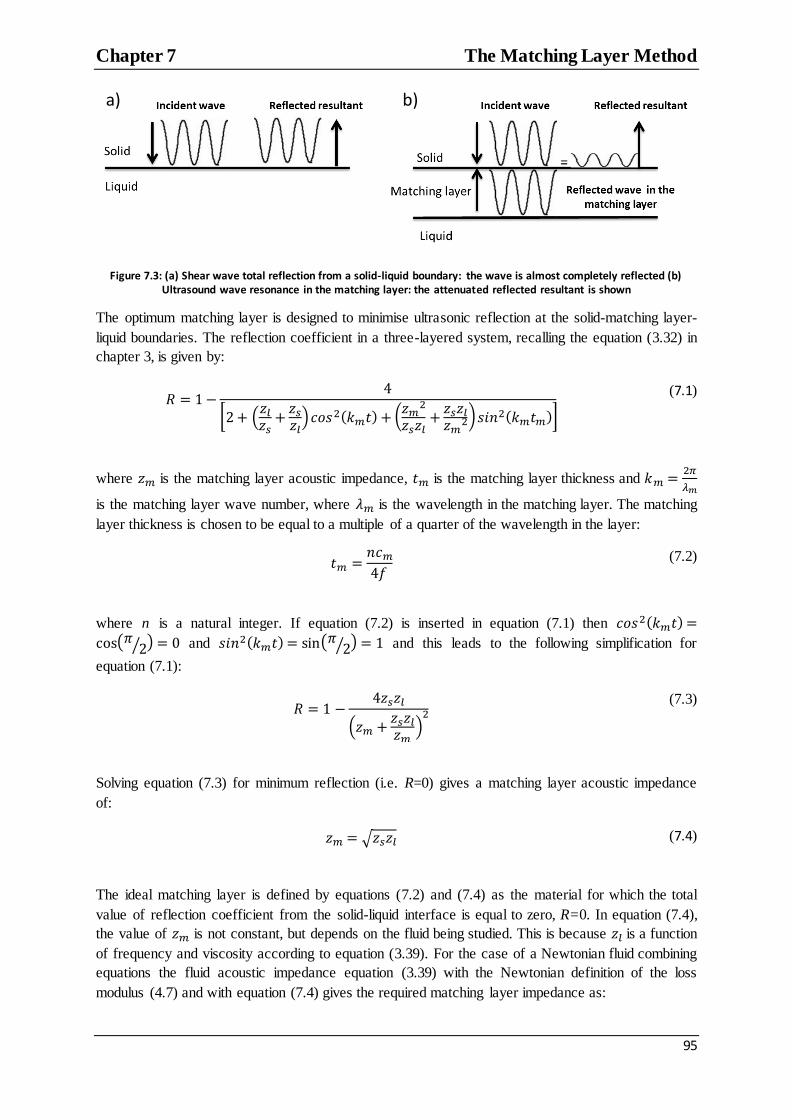
Chapter 7 The Matching Layer Method
95
Figure 7.3: (a) Shear wave total reflection from a solid-liquid boundary: the wave is almost completely reflected (b) Ultrasound wave resonance in the matching layer: the attenuated reflected resultant is shown
The optimum matching layer is designed to minimise ultrasonic reflection at the solid-matching layer-
liquid boundaries. The reflection coefficient in a three-layered system, recalling the equation (3.32) in
chapter 3, is given by:
[ (
) (
) ]
(7.1)
where is the matching layer acoustic impedance, is the matching layer thickness and
is the matching layer wave number, where 𝜆 is the wavelength in the matching layer. The matching
layer thickness is chosen to be equal to a multiple of a quarter of the wavelength in the layer:
(7.2)
where n is a natural integer. If equation (7.2) is inserted in equation (7.1) then
( ⁄ ) and ( ⁄ ) and this leads to the following simplification for
equation (7.1):
(
)
(7.3)
Solving equation (7.3) for minimum reflection (i.e. R=0) gives a matching layer acoustic impedance
of:
√ (7.4)
The ideal matching layer is defined by equations (7.2) and (7.4) as the material for which the total
value of reflection coefficient from the solid-liquid interface is equal to zero, R=0. In equation (7.4),
the value of is not constant, but depends on the fluid being studied. This is because is a function
of frequency and viscosity according to equation (3.39). For the case of a Newtonian fluid combining
equations the fluid acoustic impedance equation (3.39) with the Newtonian definition of the loss
modulus (4.7) and with equation (7.4) gives the required matching layer impedance as:
a) b)

Chapter 7 The Matching Layer Method
96
√ √ (7.5)
Equation (7.5) shows that the optimum matching layer impedance is a function of the excitation
frequency. Therefore, as well as selecting a layer to match the material properties, it is important to
match the transducer frequency bandwidth. Figure (7.4) shows the optimum matching material
acoustic impedance calculated with equation (7.5) in case of a fluid of 250 mPas viscosity, density of
900 and for the transducer frequency varying from 100kHz to 10 MHz for both aluminium,
steel or tungsten carbide solid body. For example, when measuring at 5 MHz on a steel bearing the
matching layer material should have an acoustic impedance of 1.3 MRayl. It can be noticed that the
acoustic properties of the matching layer change considerably from low to high ultrasonic
frequencies.
Figure 7.4 Optimum matching layer acoustic impedance for bearing materials of aluminium, steel and tungsten carbide coupled with an oil of viscosity 250 mPas and density 900 over a range of ultrasonic frequencies
The „ideal‟ values of the matching layer impedance and thickness (i.e. values that lead to R=0) are
given by equations (7.2) and (7.4). Figure (7.5) shows the effect of deviation from the ideal matching
layer acoustic impedance and thickness on R calculated using equation (7.1). The results are
calculated for the transducer frequency of 5 MHz and for a lubricant with viscosity of 250 mPas and
density of 900 kgm-3
. Sensitive ultrasonic measurements of fluid properties are possible when R<0.9
because a good discrimination of the different samples analysed is possible. For values greater than
0.9, the reflected signal is too close in magnitude to the incident signal and measurements suffer from
noise, as in the case where no matching layer is inserted on the wave path. The plot shows the
acceptable combinations of matching layer thicknesses. Therefore the polyimide matching layers are
suitable for all three bearing metals; whereas a lead based Babbit is on the limit for steel.
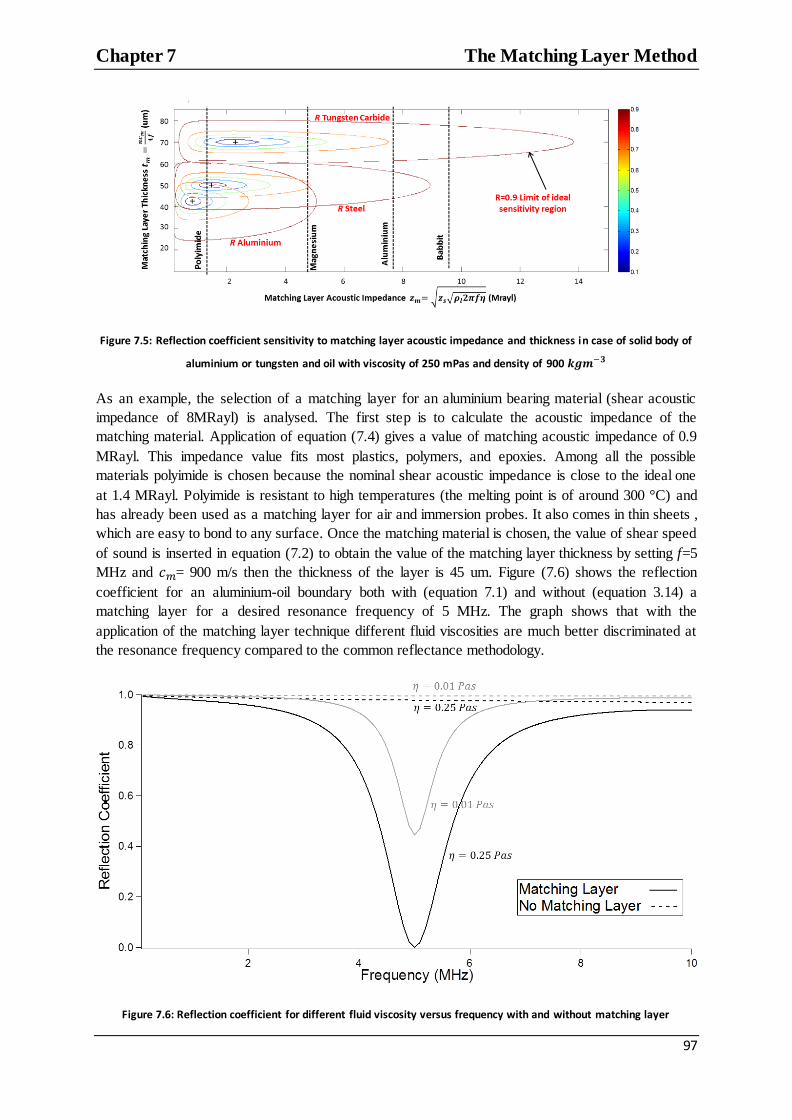
Chapter 7 The Matching Layer Method
97
Figure 7.5: Reflection coefficient sensitivity to matching layer acoustic impedance and thickness in case of solid body of
aluminium or tungsten and oil with viscosity of 250 mPas and density of 900
As an example, the selection of a matching layer for an aluminium bearing material (shear acoustic
impedance of 8MRayl) is analysed. The first step is to calculate the acoustic impedance of the
matching material. Application of equation (7.4) gives a value of matching acoustic impedance of 0.9
MRayl. This impedance value fits most plastics, polymers, and epoxies. Among all the possible
materials polyimide is chosen because the nominal shear acoustic impedance is close to the ideal one
at 1.4 MRayl. Polyimide is resistant to high temperatures (the melting point is of around 300 °C) and
has already been used as a matching layer for air and immersion probes. It also comes in thin sheets ,
which are easy to bond to any surface. Once the matching material is chosen, the value of shear speed
of sound is inserted in equation (7.2) to obtain the value of the matching layer thickness by setting f=5
MHz and = 900 m/s then the thickness of the layer is 45 um. Figure (7.6) shows the reflection
coefficient for an aluminium-oil boundary both with (equation 7.1) and without (equation 3.14) a
matching layer for a desired resonance frequency of 5 MHz. The graph shows that with the
application of the matching layer technique different fluid viscosities are much better discriminated at
the resonance frequency compared to the common reflectance methodology.
Figure 7.6: Reflection coefficient for different fluid viscosity versus frequency with and without matching layer

Chapter 7 The Matching Layer Method
98
7.3 Measurement Apparatus
7.3.1 Instrumentation
Figure (7.7) schematically shows the measurement instrumentation. A pair of ultrasonic piezoelectric
(PZT) shear mode transducers operate in pulse-echo mode at a centre frequency of 10 MHz. One
transducer produces the ultrasonic wave (transmitter) and the second receives the echo wave
(receiver). The pulser is excited by a signal produced by an arbitrary waveform function generator
(TTI TG5011). Once excited by the electric signal, the pulser vibrates, emitting an ultrasonic wave
that propagates through the solid until it is incident on the solid-liquid interface, where part of the
wave is transmitted and part is reflected back. The reflected signal is received by the receiver sensor
and the signal is recorded on an oscilloscope (LeCroy LT342) with a sampling capacity of 500 MS/s,
continuously analysed, and stored in real time using an acquisition interface written in LabView™.
The LabView™ routine is the same as the one described in chapter 6.
Figure 7.7: Schematic diagram of the measurement apparatus
7.3.2 Test Cell and Matching Layer
Figure (7.8) shows the ultrasonic probe that consists of an aluminium plate 20 mm thick, exactly like
the one described in section (6.1), with the ultrasonic transducers bonded underneath. A top solid
plate is used to enclose the oil sample in a thin film set-up and has holes that allow positioning K-type
thermocouples in direct contact with the fluid. Figure (7.8a) shows the 50um polyimide matching
layer bonded on the aluminium surface. The choice of the matching layer is based on equations (7.2)
and (7.4) and is described in detail in the example in section 7.2.

Chapter 7 The Matching Layer Method
99
Figure 7.8 a) Ultrasonic test cell. (b) Ultrasonic transducers
7.3.3 Samples Tested
The same Cannon™ standard viscosity mineral oils were tested along with a selection of engine
lubricants. Table 7.1 gives the viscosity data for the samples tested. The engine lubricants were
selected from common mixtures and compounds used in automotive engines. The oils VM1 and VM2
refer to fully formulated engine lubricants with two different viscosity modifiers while the Detergents
refer to oils with different TBN (total base number). The viscosity of all the oils has been measured
with a cone viscometer at at three temperatures. Three values of viscosity at different
temperature are needed to apply the Vogel equation (equation (2.5)) to obtain accurate reference
viscosity values in case the ultrasonic acquisition is done outside the tabled viscosity values for the
Cannon™ standards.
Oil Type Oil Sample Viscosity (mPas) @25°C
Viscosity (mPas) @40°C
Viscosity (mPas) @50°C
Mineral Oils
S20 29.1 15.3 10.7 N35 55.9 27.1 18.1
N100 200.7 83.1 50.5 S200 407.6 155.8 92.3
S600 1329 446.2 240.4
Synthetic Oils PAO 8 89.7 43.1 31.4
PAO 40 914 349.2 231.3 PAO 100 3540 1218 765.2
Fully Formulated
Engine Oils
VM1 246.9 102.6 71.1 VM2 118.2 57.3 41.9
High Detergent 84.7 41.5 31.0 Low Detergent 116.2 51.6 36.1
ESTER 234.2 99.2 69.3 Table 7.1: Samples tested and the viscosities measured with a cone viscometer at a shear rate of
7.4 Signal Processing and Data Analysis
The frequency dependent reflected amplitude spectrum is initially obtained when there is no oil
present (reference acquisition). Since almost all the wave is reflected back non-attenuated at an air
interface, this signal is equal to the incident signal and serves as a reference. All subsequent
measurements from solid-liquid interfaces, , are divided by this reference to give the reflection
Matching Layer

Chapter 7 The Matching Layer Method
100
coefficient, R. The pulsing signal employed is a chirp as shown in Figure (7.9). This is a signal
modulated in frequency; which means that with a single chirp burst it is possible to excite a range of
different frequencies.
Figure 7.9: Chirp pulse 3-10 MHz, time domain representation
The chirp ensures that the matching layer resonance frequency is found precisely. Figure (7.10 a)
shows the applicable frequency spectrum of the reflected pulse from the setup shown in Figure (7.8)
when there is a fluid sample in a contact and when it is absent.
Figure 7.10: a) Chirp FFT for measurement and calibration reference. b) Reflection coefficient: it is highlighted the
increment in sensitivity at the resonance frequency, while outside resonance the reflection coefficient approaches 1
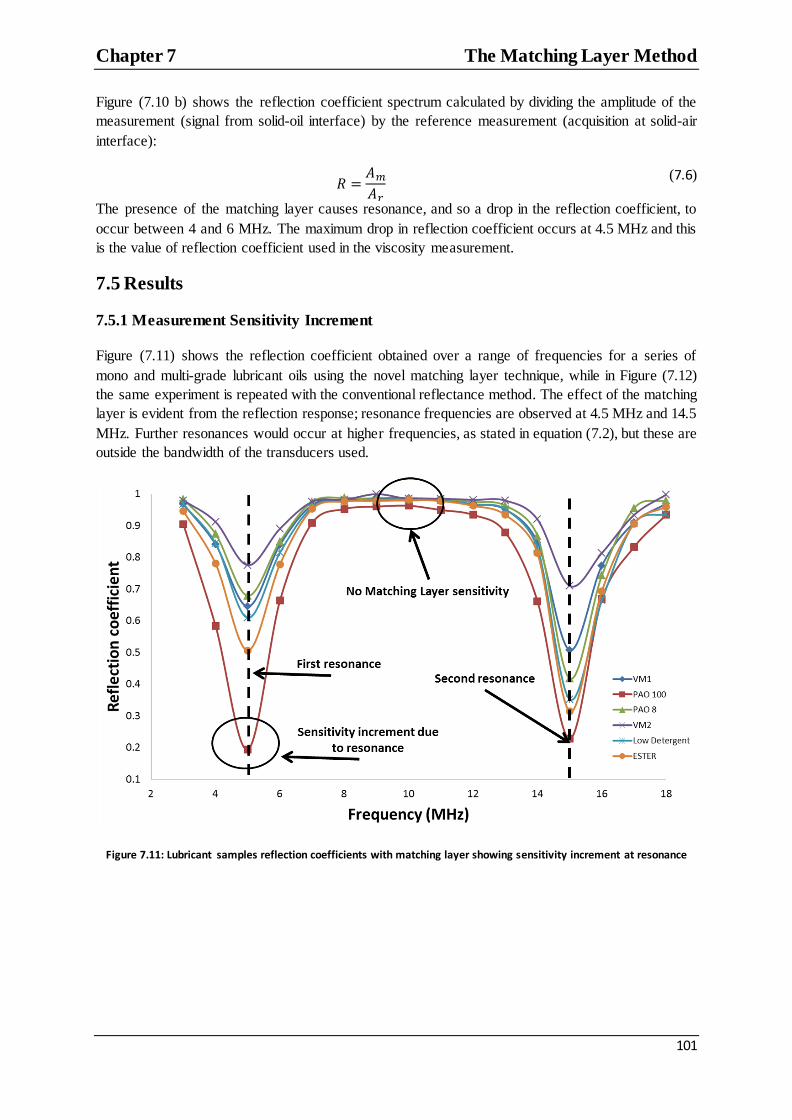
Chapter 7 The Matching Layer Method
101
Figure (7.10 b) shows the reflection coefficient spectrum calculated by dividing the amplitude of the
measurement (signal from solid-oil interface) by the reference measurement (acquisition at solid-air
interface):
(7.6)
The presence of the matching layer causes resonance, and so a drop in the reflection coefficient, to
occur between 4 and 6 MHz. The maximum drop in reflection coefficient occurs at 4.5 MHz and this
is the value of reflection coefficient used in the viscosity measurement.
7.5 Results
7.5.1 Measurement Sensitivity Increment
Figure (7.11) shows the reflection coefficient obtained over a range of frequencies for a series of
mono and multi-grade lubricant oils using the novel matching layer technique, while in Figure (7.12)
the same experiment is repeated with the conventional reflectance method. The effect of the matching
layer is evident from the reflection response; resonance frequencies are observed at 4.5 MHz and 14.5
MHz. Further resonances would occur at higher frequencies, as stated in equation (7.2), but these are
outside the bandwidth of the transducers used.
Figure 7.11: Lubricant samples reflection coefficients with matching layer showing sensitivity increment at resonance

Chapter 7 The Matching Layer Method
102
Figure 7.12: Lubricant sample reflection coefficients acquired with the conventional ultrasonic reflectance technique
In Figure (7.11) the response of the different lubricants at the resonance frequency is well
discriminated. Away from the resonance frequencies, for example at 10 MHz, all the lubricant films
show a reflection close to one and it is hard to discriminate between them. In this region the matching
layer has no beneficial effect on the reflection because the incident wave and the reflected wave from
the matching layer are not in phase and total reflection happens just as in the case where no matching
layer is inserted present. This is shown schematically in Figure (7.13).
Figure 7.13: On the left the cancellation effect at the resonance frequency that reduces the overall reflected energy, on the right the ultrasonic wave is incident at a frequency for which the reflection from the matching layer is out of phase;
as a consequence total reflection occurs
The graph in Figure (7.11) shows the importance of the matching layer technique. Without the
matching layer the response would be similar to that which occurs at 10 MHz across the whole
frequency spectrum. Table 7.2 reports the reflection coefficient at the first resonance frequency, 4.5
MHz, and away from resonance, at 10 MHz. The reported values are obtained from the mean of five
experimental repetitions.

Chapter 7 The Matching Layer Method
103
Frequency (MHz) Sample Mean Reflection coefficient Standard Deviation
4.5
VM1 0.634 0.011 VM2 0.784 0.011
PAO 8 0.687 0.013
PAO 100 0.200 0.015 High Detergent 0.607 0.020
ESTER 0.515 0.012
10
VM1 0.986 0.012
VM2 0.984 0.014 PAO 8 0.983 0.015
PAO 100 0.962 0.015
High Detergent 0.979 0.017 ESTER 0.981 0.018
Table 7.2. Sensitivity increment at resonance
This table, which can be compared with Table 6.2, shows that the matching layer technique does not
improve the accuracy of the ultrasound method, but increases the sensitivity to fluid viscosity. The
standard deviation in the reflection coefficient is in fact equivalent to around 1% for both the cases,
but in the case of resonance the error of ±1% it is acceptable, while outside resonance the same error
makes impossible to distinguish between different samples. This happens because the electrical
instrumentation and the acquisition tools have not been changed compared to the setup in section 6
and so the uncertainty in the ultrasound signal acquisition has not changed compared to the previous
setup while only the sensitivity to fluid characteristic is enhanced by the insertion of the matching
layer.
7.5.2 Viscosity Results for Newtonian Oils
Figure (7.14) shows the reflection coefficients acquired for a set of Cannon™ calibrated mineral oils
(see section 6.1) around the resonance frequency. The mineral oils were chosen for their Newtonian
behaviour, which is ideal to test the efficiency of the ultrasonic viscometer.
Figure 7.14: Reflection coefficient at resonance for calibrated Newtonian oils
The reflection coefficient values at 4.5 MHz were used in equation (5.14) to obtain the oil viscosity.
Figure (7.15) shows viscosities measured with the ultrasonic method plotted against the viscosity

Chapter 7 The Matching Layer Method
104
determined using a conventional cone viscometer. This plot shows the excellent agreement between
the predicted and measured data with a correlation coefficient of R2=0.999.
Figure 7.15: Ultrasonic viscometer versus conventional cone viscometer plot
7.5.3 The Empirical Correlation Between Viscosity and Reflection Coefficient
Figure (7.16) shows the reflection coefficient plotted against the viscosity values measured with a
conventional cone viscometer for the tested mineral oils. The Maxwell, Greenwood and Newtonian
models of reflection, given respectively as equations (5.14, 4.9 and 4.15), are plotted as well. For the
different algorithms the values of reflection coefficient reported in chapter 7.5.2 are converted to
viscosity. It can be noticed that the experimental results and the Maxwell model are in very good
agreement, while the Newtonian model shear thins for values of viscosity >0.1 Pas and the
Greenwood model gives shear thickened values for viscosity values >0.1 Pas.
Figure 7.16 Relationship between reflection coefficient and viscosity for standard mineral oils. The experimental data are close to the Maxwell model and a logarithmic fit.

Chapter 7 The Matching Layer Method
105
The Maxwell model, equation (5.14), contains some parameters, like fluid density and the oil acoustic
impedance, that need to be measured in order to convert R to viscosity. Another approach for
determining the relationship between viscosity and reflection coefficient would be to calibrate a
particular list of known viscosity Newtonian oils by curve fitting pairs of ( ,R) experimental data
points. As it can be seen in Figure (7.16), a logarithmic relation fit to the data points:
( √
)
(7.7)
Where the coefficients of equations (7.7) have the following values:
Coefficient Value 0.98305
-0.92349
21.198
4.9335 Table 7.3: Coefficient of the logarithmic fit function, equation (7.7)
The logarithmic fit was chosen because it guarantees the maximum correlation with the experimental
data point. Moreover, it can be noticed that there is a strong correlation between the theoretical
Maxwell model and the empirical fit. This means that viscosity could be measured by knowing only
the reflection coefficient. In fact, this type of empirical law does not need the prior knowledge of any
fluid properties to determine the viscosity, but only the measured reflection coefficient. It is then not
affected by any error due to the evaluation of the fluid density and the solid and liquid acoustic
impedances. The values of the coefficients reported in table (7.3) are dependent on the transducers
characteristics and vary when the ultrasonic set-up change.
The empirical law could be implemented as follows. The first step consists of calibrating the
ultrasonic probe with respect to Newtonian oils, for which it is possible to make a viscosity-reflection
coefficient graph as the one shown in Figure (7.16). Newtonian oils have to be chosen so that the
calibration graph is not dependent on the operating frequency. After the reflection coefficient-
viscosity curve is obtained, this is interpolated and the function is used to measure viscosity in the in-
situ test. This method is used in chapter 8 to obtain viscosity in the journal bearing test rig.
7.5.3 Viscosity Results for Fully Formulated Engine Oils
The reflection coefficient data for the formulated engine lubricants reported in Table (7.2) were
converted into viscosity using equation (7.7). Figure (7.17) reports the comparison of the viscosity
measured with the ultrasonic method for fully formulated engine lubricants against the viscosity
measured with a cone viscometer at 102 s
-1.
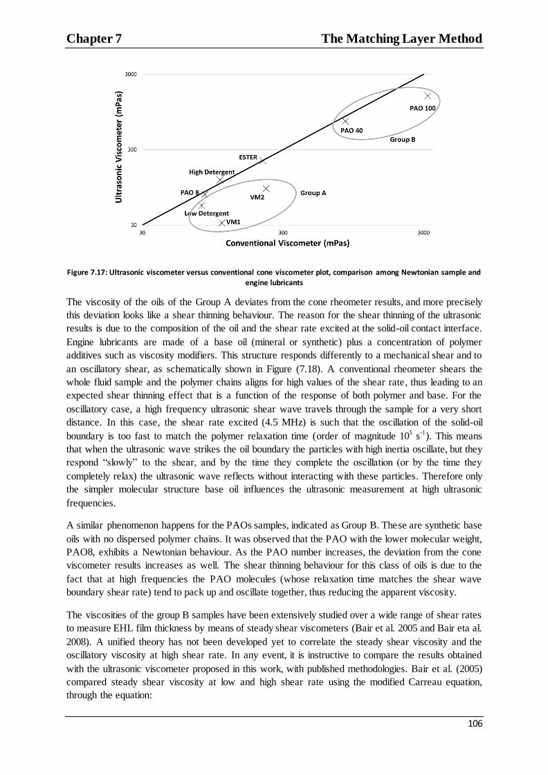
Chapter 7 The Matching Layer Method
106
Figure 7.17: Ultrasonic viscometer versus conventional cone viscometer plot, comparison among Newtonian sample and engine lubricants
The viscosity of the oils of the Group A deviates from the cone rheometer results, and more precisely
this deviation looks like a shear thinning behaviour. The reason for the shear thinning of the ultrasonic
results is due to the composition of the oil and the shear rate excited at the solid-oil contact interface.
Engine lubricants are made of a base oil (mineral or synthetic) plus a concentration of polymer
additives such as viscosity modifiers. This structure responds differently to a mechanical shear and to
an oscillatory shear, as schematically shown in Figure (7.18). A conventional rheometer shears the
whole fluid sample and the polymer chains aligns for high values of the shear rate, thus leading to an
expected shear thinning effect that is a function of the response of both polymer and base. For the
oscillatory case, a high frequency ultrasonic shear wave travels through the sample for a very short
distance. In this case, the shear rate excited (4.5 MHz) is such that the oscillation of the solid-oil
boundary is too fast to match the polymer relaxation time (order of magnitude 105 s
-1). This means
that when the ultrasonic wave strikes the oil boundary the particles with high inertia oscillate, but they
respond “slowly” to the shear, and by the time they complete the oscillation (or by the time they
completely relax) the ultrasonic wave reflects without interacting with these particles. Therefore only
the simpler molecular structure base oil influences the ultrasonic measurement at high ultrasonic
frequencies.
A similar phenomenon happens for the PAOs samples, indicated as Group B. These are synthetic base
oils with no dispersed polymer chains. It was observed that the PAO with the lower molecular weight,
PAO8, exhibits a Newtonian behaviour. As the PAO number increases, the deviation from the cone
viscometer results increases as well. The shear thinning behaviour for this class of oils is due to the
fact that at high frequencies the PAO molecules (whose relaxation time matches the shear wave
boundary shear rate) tend to pack up and oscillate together, thus reducing the apparent viscosity.
The viscosities of the group B samples have been extensively studied over a wide range of shear rates
to measure EHL film thickness by means of steady shear viscometers (Bair et al. 2005 and Bair eta al.
2008). A unified theory has not been developed yet to correlate the steady shear viscosity and the
oscillatory viscosity at high shear rate. In any event, it is instructive to compare the results obtained
with the ultrasonic viscometer proposed in this work, with published methodologies. Bair et al. (2005)
compared steady shear viscosity at low and high shear rate using the modified Carreau equation,
through the equation:
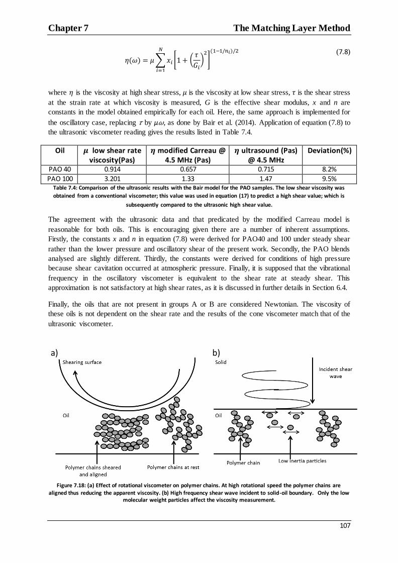
Chapter 7 The Matching Layer Method
107
𝜔 ∑ * (𝜏
)
+
(7.8)
where is the viscosity at high shear stress, is the viscosity at low shear stress, 𝜏 is the shear stress
at the strain rate at which viscosity is measured, G is the effective shear modulus, x and n are
constants in the model obtained empirically for each oil. Here, the same approach is implemented for
the oscillatory case, replacing 𝜏 by μ𝜔, as done by Bair et al. (2014). Application of equation (7.8) to
the ultrasonic viscometer reading gives the results listed in Table 7.4.
Oil low shear rate viscosity(Pas)
modified Carreau @ 4.5 MHz (Pas)
ultrasound (Pas) @ 4.5 MHz
Deviation(%)
PAO 40 0.914 0.657 0.715 8.2%
PAO 100 3.201 1.33 1.47 9.5% Table 7.4: Comparison of the ultrasonic results with the Bair model for the PAO samples. The low shear viscosity was
obtained from a conventional viscometer; this value was used in equation (17) to predict a high shear value; which is
subsequently compared to the ultrasonic high shear value.
The agreement with the ultrasonic data and that predicated by the modified Carreau model is
reasonable for both oils. This is encouraging given there are a number of inherent assumptions.
Firstly, the constants x and n in equation (7.8) were derived for PAO40 and 100 under steady shear
rather than the lower pressure and oscillatory shear of the present work. Secondly, the PAO blends
analysed are slightly different. Thirdly, the constants were derived for conditions of high pressure
because shear cavitation occurred at atmospheric pressure. Finally, it is supposed that the vibrational
frequency in the oscillatory viscometer is equivalent to the shear rate at steady shear. This
approximation is not satisfactory at high shear rates, as it is discussed in further details in Section 6.4.
Finally, the oils that are not present in groups A or B are considered Newtonian. The viscosity of
these oils is not dependent on the shear rate and the results of the cone viscometer match that of the
ultrasonic viscometer.
Figure 7.18: (a) Effect of rotational viscometer on polymer chains. At high rotational speed the polymer chains are
aligned thus reducing the apparent viscosity. (b) High frequency shear wave incident to solid-oil boundary. Only the low molecular weight particles affect the viscosity measurement.
a) b)

Chapter 7 The Matching Layer Method
108
7.6 Effect of Polymer Concentration and Excitation Frequency
In chapter 4, it was reported that several researchers compared viscosity from an oscillatory shear and
a mechanical induced continuous shear (Cox and Merz, 1958, Laun, 1986 and Al-Hadithi et al.,
1992). Cox and Merz introduced a generally accepted empirical rule to compare the shear strain of
conventional viscometers and oscillatory based ones:
𝜔 | (7.9)
where is the shear strain from a conventional rotational viscometer and 𝜔 is the rotational
frequency. This rule states that the rotational frequency of an oscillatory based viscometer is equal to
the shear strain at the solid-liquid boundary and that the measurement made with such technique is
comparable with the reading from a conventional rheometer. In chapter 4 this rule was shown to be
valid up to 104 Hz. At high shear rates this is no longer, especially for polymer based oils. Larson
(1988) stated regarding the viscosity measurement of polymers executed with an oscillatory
technique: “In the bead and spring description, a polymer molecule contributes nothing to the viscous
dissipation if the deformation is too fast. In this limit, the dilute solution acts as a suspension of rigid
particles, and the viscosity is constant”. This statement was validated by the results shown in the
previous section. Similarly Laun (1986) proposed another model to correlate the steady state
mechanical shear rate to the vibrational shear rate:
(
𝜔)[ (
)
]
|
(7.10)
where is the normal stress difference coefficient measured in steady shear. Both rules by Cox and
Laun were analysed by Wen et al. (2004) at low shear rates (up to Hz). It was demonstrated that
the rules are valid in the shear rate range ( s-1
), thought deviation from the measured steady
state shear rate begins at the higher frequency. A similar comparison was conducted numerically by
Sharma and McKinley (2013). Bair (2014) first applied the Cox-Merz rule at high rotational
frequencies (107
Hz) using an impedance spectrometer microbalance, and discovered that for the
polymer based oils tested this rule is no longer valid. The matching layer ultrasound viscometer
results in section 6.3 show the same behaviour. This is confirmed by comparing the measurements
taken using an ultra-high shear viscometer (the USV by PCS instruments) and the proposed ultrasonic
viscometer. The different mixtures with the same base oil and different polymer concentrations were
tested at a shear rate of 4.5 MHz. Table (7.5) reports the mixture polymer content and viscosity
measured with both the UHSV and the ultrasonic viscometer at 4.5 MHz at 100°C.
Sample Base (%)
Polymer concentration (%)
Viscosity (mPas)
@100°C [UHSV,4.5* s-1]
Viscosity (mPas)
@100°C [Ultrasound,4.5 MHz]
Base 1 100 0 6.18 6.11
Mixture 1 99.5 0.5 6.73 6.20
Mixture 2 99 1 7.72 6.16
Mixture 3 98 2 12.43 6.29
Table 7.5: Polymer concentration and viscosity of several custom mixtures
Figure (7.19) shows that the ultrasonic viscometer reading is coincident with the viscosity of the base
(0% polymer concentration). These results demonstrate that the lubricants are sheared too quickly by
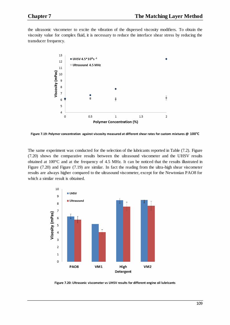
Chapter 7 The Matching Layer Method
109
the ultrasonic viscometer to excite the vibration of the dispersed viscosity modifiers. To obtain the
viscosity value for complex fluid, it is necessary to reduce the interface shear stress by reducing the
transducer frequency.
Figure 7.19: Polymer concentration against viscosity measured at different shear rates for custom mixtures @ 100°C
The same experiment was conducted for the selection of the lubricants reported in Table (7.2). Figure
(7.20) shows the comparative results between the ultrasound viscometer and the UHSV results
obtained at 100°C and at the frequency of 4.5 MHz. It can be noticed that the results illustrated in
Figure (7.20) and Figure (7.19) are similar. In fact the reading from the ultra-high shear viscometer
results are always higher compared to the ultrasound viscometer, except for the Newtonian PAO8 for
which a similar result is obtained.
Figure 7.20: Ultrasonic viscometer vs UHSV results for different engine oil lubricants
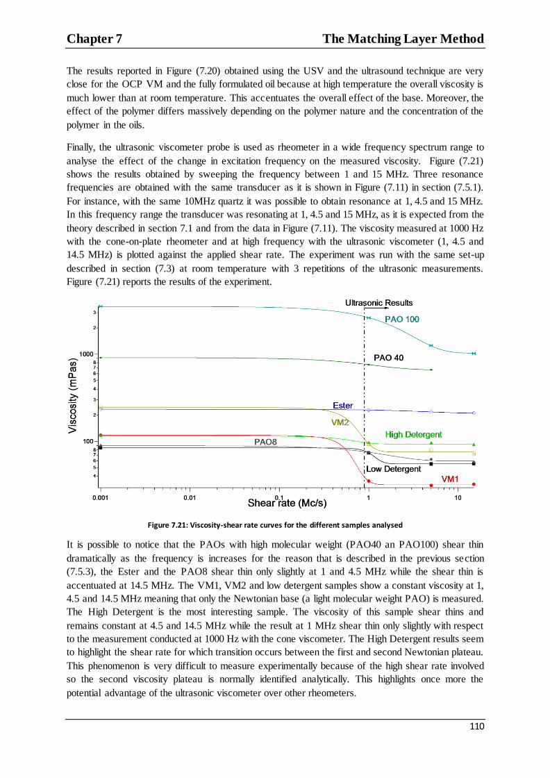
Chapter 7 The Matching Layer Method
110
The results reported in Figure (7.20) obtained using the USV and the ultrasound technique are very
close for the OCP VM and the fully formulated oil because at high temperature the overall viscosity is
much lower than at room temperature. This accentuates the overall effect of the base. Moreover, the
effect of the polymer differs massively depending on the polymer nature and the concentration of the
polymer in the oils.
Finally, the ultrasonic viscometer probe is used as rheometer in a wide frequency spectrum range to
analyse the effect of the change in excitation frequency on the measured viscosity. Figure (7.21)
shows the results obtained by sweeping the frequency between 1 and 15 MHz. Three resonance
frequencies are obtained with the same transducer as it is shown in Figure (7.11) in section (7.5.1).
For instance, with the same 10MHz quartz it was possible to obtain resonance at 1, 4.5 and 15 MHz.
In this frequency range the transducer was resonating at 1, 4.5 and 15 MHz, as it is expected from the
theory described in section 7.1 and from the data in Figure (7.11). The viscosity measured at 1000 Hz
with the cone-on-plate rheometer and at high frequency with the ultrasonic viscometer (1, 4.5 and
14.5 MHz) is plotted against the applied shear rate. The experiment was run with the same set-up
described in section (7.3) at room temperature with 3 repetitions of the ultrasonic measurements.
Figure (7.21) reports the results of the experiment.
Figure 7.21: Viscosity-shear rate curves for the different samples analysed
It is possible to notice that the PAOs with high molecular weight (PAO40 an PAO100) shear thin
dramatically as the frequency is increases for the reason that is described in the previous section
(7.5.3), the Ester and the PAO8 shear thin only slightly at 1 and 4.5 MHz while the shear thin is
accentuated at 14.5 MHz. The VM1, VM2 and low detergent samples show a constant viscosity at 1,
4.5 and 14.5 MHz meaning that only the Newtonian base (a light molecular weight PAO) is measured.
The High Detergent is the most interesting sample. The viscosity of this sample shear thins and
remains constant at 4.5 and 14.5 MHz while the result at 1 MHz shear thin only slightly with respect
to the measurement conducted at 1000 Hz with the cone viscometer. The High Detergent results seem
to highlight the shear rate for which transition occurs between the first and second Newtonian plateau.
This phenomenon is very difficult to measure experimentally because of the high shear rate involved
so the second viscosity plateau is normally identified analytically. This highlights once more the
potential advantage of the ultrasonic viscometer over other rheometers.
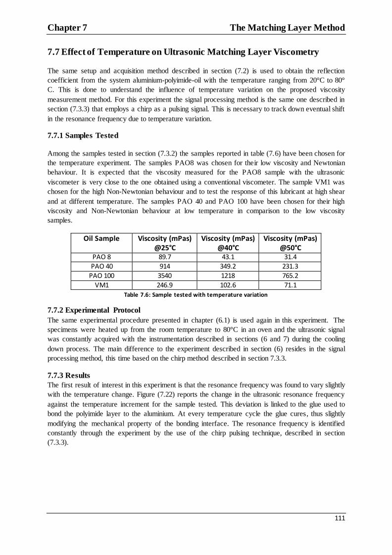
Chapter 7 The Matching Layer Method
111
7.7 Effect of Temperature on Ultrasonic Matching Layer Viscometry
The same setup and acquisition method described in section (7.2) is used to obtain the reflection
coefficient from the system aluminium-polyimide-oil with the temperature ranging from 20°C to 80°
C. This is done to understand the influence of temperature variation on the proposed viscosity
measurement method. For this experiment the signal processing method is the same one described in
section (7.3.3) that employs a chirp as a pulsing signal. This is necessary to track down eventual shift
in the resonance frequency due to temperature variation.
7.7.1 Samples Tested
Among the samples tested in section (7.3.2) the samples reported in table (7.6) have been chosen for
the temperature experiment. The samples PAO8 was chosen for their low viscosity and Newtonian
behaviour. It is expected that the viscosity measured for the PAO8 sample with the ultrasonic
viscometer is very close to the one obtained using a conventional viscometer. The sample VM1 was
chosen for the high Non-Newtonian behaviour and to test the response of this lubricant at high shear
and at different temperature. The samples PAO 40 and PAO 100 have been chosen for their high
viscosity and Non-Newtonian behaviour at low temperature in comparison to the low viscosity
samples.
Oil Sample Viscosity (mPas) @25°C
Viscosity (mPas) @40°C
Viscosity (mPas) @50°C
PAO 8 89.7 43.1 31.4
PAO 40 914 349.2 231.3
PAO 100 3540 1218 765.2
VM1 246.9 102.6 71.1
Table 7.6: Sample tested with temperature variation
7.7.2 Experimental Protocol
The same experimental procedure presented in chapter (6.1) is used again in this experiment. The
specimens were heated up from the room temperature to 80°C in an oven and the ultrasonic signal
was constantly acquired with the instrumentation described in sections (6 and 7) during the cooling
down process. The main difference to the experiment described in section (6) resides in the signal
processing method, this time based on the chirp method described in section 7.3.3.
7.7.3 Results
The first result of interest in this experiment is that the resonance frequency was found to vary slightly
with the temperature change. Figure (7.22) reports the change in the ultrasonic resonance frequency
against the temperature increment for the sample tested. This deviation is linked to the glue used to
bond the polyimide layer to the aluminium. At every temperature cycle the glue cures, thus slightly
modifying the mechanical property of the bonding interface. The resonance frequency is identified
constantly through the experiment by the use of the chirp pulsing technique, described in section
(7.3.3).

Chapter 7 The Matching Layer Method
112
Figure 7.22: Resonance frequency deviation with temperature
Figure (7.11) shows that the frequency bandwidth for which high sensitivity is achieved ranges from 4
to 6 MHz, with the resonance frequency around 4.5 MHz. Consequently, a deviation of less than 200
kHz does not affect the sensitivity or the results of this experiment. The change in the resonance
frequency has to be taken into consideration when working at lower ultrasonic frequencies. In this
situation the sensitivity bandwidth is expected to be smaller, as it is shown in the graph in Figure
(7.5). The resonance shift is also important in experiments where the temperature gradient is high
because this might lead to higher deviations than the one shown in Figure (7.22). The use of the chirp
technique allows keeping track of the resonance change thus being ideal for working at lower
frequencies. Direct coating of the matching layer on the solid surface would make it possible to limit
this resonance frequency shift.
The reflection coefficients are acquired exactly as for the experiment described in Chapter 6and are
converted to viscosity using the Maxwell model (5.14). Figure (7.23a-d) shows the temperature-
viscosity plot for the samples tested. It is possible to notice that for the PAO8 lubricant (Figure 7.23a)
the ultrasonic results are in line with the conventional viscometer reading while the ultrasonic
measurement for the thickest lubricants shear thin compared to the conventional viscometer results.

Chapter 7 The Matching Layer Method
113
Figure 7.23: Temperature-viscosity graphs for a) PAO8, b) VM1, c) PAO 40, d) PAO100
The results show also that as the temperature is increased the reading from the ultrasonic viscometer
and cone-to-plate viscometer converges. This is shown for the case of Figure (7.23b) and for Figure
(7.23d). For the VM1 lubricant, Figure (7.23b) this is due to the fact that at high temperature the
polymer chains tend to “untangle” thus reducing the overall resistance to shear. The results of this
experiment can then be used to separate the contribution of the base and the polymer to the overall
viscosity at different temperature, as shown in Figure (7.24).
Figure 7.24: The ultrasonic viscometer measurement allow separating the viscosity of the base from the viscosity of the
polymer

Chapter 7 The Matching Layer Method
114
The ultrasonic viscometer results for the PAO100 in Figure (7.23d) converge to the classic rheometer
results because of the chemical composition of the PAO sample and its response to the different shear
stresses. The PAO100 does not have any dispersed polymer in it, but has a very complex structure that
confers a Non-Newtonian behaviour to this base oil. In particular, the molecules of the PAO tend to
align at high shear rate. This is typical in shear thin fluids and because of this the viscosity measured
at 4.5 MHz with the ultrasonic viscometer is less than the one measured with the cone viscometer at
100 Hz. This difference is less accentuated at high temperature because the molecule reticule of the
PAO stretches thus offering a minor resistance to motion at low and high shear rate.
7.8 Effect of Pressure on Ultrasonic Matching Layer Viscometry
The effect of pressure was tested in the range 0-50 MPa. This is, in fact, the range of pressures that are
expected in a journal bearing. Non-conformal contact occurs in journal bearings and so the operating
pressures are not as high as, for examples, in ball bearings (pressures up to 3 GPa). The pressure test
rig, described in detail in section 7.8.1, is made of a close cylinder where the fluid is pressurized. The
vessel is made of aluminium and a polyimide layer is used as matching layer in contact with the fluid.
This setup allowed acquiring the ultrasonic signal with high sensitivity as the fluid is pressurized. The
acquired reflection coefficient was converted in viscosity, relaxation time and complex shear modulus
using the Maxwell model (equation 5.12).
7.8.1 Materials
Figure (7.25) shows schematically the pressure test rig measurement chain. The ultrasonic pulsing-
receiving acquisition apparatus is the same as the one used in previous experiments. The oil samples
are pressurised inside a closed cylinder by an Enerpac hydraulic hand pump that can reach up to the
maximum pressure of 70 MPa. The pump is connected to the cylinder through a hydraulic sealed
connection. Figure (7.26) shows the cylinder design in more detail. The cylinder is made of EN24T
grade steel and the wall is 20 mm thick. The cylinder contains a volume of 0.0045 . Inside the
cylinder the lubricant is contained in a thin film chamber machined to have an overall thickness of 50
micron.
Figure 7.25: Pressure test rig measurement chain

Chapter 7 The Matching Layer Method
115
Figure (7.27) shows a picture of the thin film chamber test cell along with the vessel and the localizer.
The thin film chamber is a cylindrical element with three channels that allow the lubricant to fill a
cavity of 50 micron depth. This was done to recreate the same thin film setup described in Chapter 6.
The localizer is a component that centres the test cell with respect to the centre of the vessel and the
ultrasonic transducers. In this way, the ultrasonic wave is localised always at the solid-thin film
interface. The assembly of the vessel, the localizer and the thin film chamber is shown in Figures
(7.26) and (7.28). The ultrasonic transducers are 5 MHz PZ-5A ultrasonic bare elements and are
located on the top of the vessel, as shown in Figure (7.26). The vessel is made of aluminium and at the
bottom of the vessel a 50 um polyimide layer is bonded to act as a matching layer just like described
in Chapter 7.
Figure 7.26: Schematic representation of the pressure rig and the vessell assembly
Figure 7.27: The vessel, the thin film chamber and the localizer
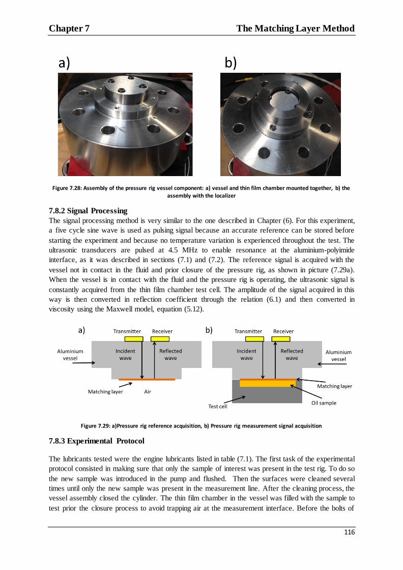
Chapter 7 The Matching Layer Method
116
Figure 7.28: Assembly of the pressure rig vessel component: a) vessel and thin film chamber mounted together, b) the
assembly with the localizer
7.8.2 Signal Processing
The signal processing method is very similar to the one described in Chapter (6). For this experiment,
a five cycle sine wave is used as pulsing signal because an accurate reference can be stored before
starting the experiment and because no temperature variation is experienced throughout the test. The
ultrasonic transducers are pulsed at 4.5 MHz to enable resonance at the aluminium-polyimide
interface, as it was described in sections (7.1) and (7.2). The reference signal is acquired with the
vessel not in contact in the fluid and prior closure of the pressure rig, as shown in picture (7.29a).
When the vessel is in contact with the fluid and the pressure rig is operating, the ultrasonic signal is
constantly acquired from the thin film chamber test cell. The amplitude of the signal acquired in this
way is then converted in reflection coefficient through the relation (6.1) and then converted in
viscosity using the Maxwell model, equation (5.12).
Figure 7.29: a)Pressure rig reference acquisition, b) Pressure rig measurement signal acquisition
7.8.3 Experimental Protocol
The lubricants tested were the engine lubricants listed in table (7.1). The first task of the experimental
protocol consisted in making sure that only the sample of interest was present in the test rig. To do so
the new sample was introduced in the pump and flushed. Then the surfaces were cleaned several
times until only the new sample was present in the measurement line. After the cleaning process, the
vessel assembly closed the cylinder. The thin film chamber in the vessel was filled with the sample to
test prior the closure process to avoid trapping air at the measurement interface. Before the bolts of
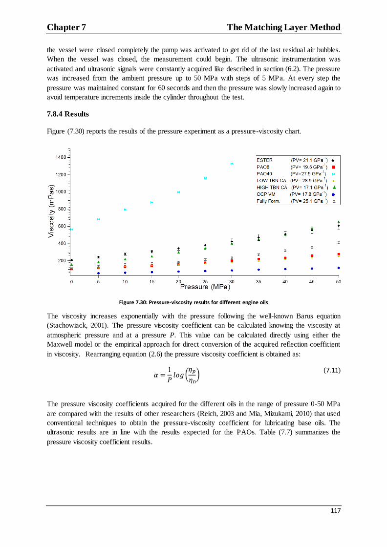
Chapter 7 The Matching Layer Method
117
the vessel were closed completely the pump was activated to get rid of the last residual air bubbles.
When the vessel was closed, the measurement could begin. The ultrasonic instrumentation was
activated and ultrasonic signals were constantly acquired like described in section (6.2). The pressure
was increased from the ambient pressure up to 50 MPa with steps of 5 MPa. At every step the
pressure was maintained constant for 60 seconds and then the pressure was slowly increased again to
avoid temperature increments inside the cylinder throughout the test.
7.8.4 Results
Figure (7.30) reports the results of the pressure experiment as a pressure-viscosity chart.
Figure 7.30: Pressure-viscosity results for different engine oils
The viscosity increases exponentially with the pressure following the well-known Barus equation
(Stachowiack, 2001). The pressure viscosity coefficient can be calculated knowing the viscosity at
atmospheric pressure and at a pressure P. This value can be calculated directly using either the
Maxwell model or the empirical approach for direct conversion of the acquired reflection coefficient
in viscosity. Rearranging equation (2.6) the pressure viscosity coefficient is obtained as:
(
) (7.11)
The pressure viscosity coefficients acquired for the different oils in the range of pressure 0-50 MPa
are compared with the results of other researchers (Reich, 2003 and Mia, Mizukami, 2010) that used
conventional techniques to obtain the pressure-viscosity coefficient for lubricating base oils. The
ultrasonic results are in line with the results expected for the PAOs. Table (7.7) summarizes the
pressure viscosity coefficient results.

Chapter 7 The Matching Layer Method
118
Lubricant Pressure viscosity coefficient ultrasonic
viscometer ( )
Pressure viscosity coefficient literature
( )
Literature reference
PAO 8 19.5 11-18 (@ 40 °C) Reich (2003), Mia (2010), Roelands (1966) PAO 40 27.5 14-20 (@ 40 °C)
ESTER 21.1 16-21 (@40 °C) Roelands (1966)
High TBN 28.9 - -
Low TBN 17.1 - -
OCP VM 17.8 - -
Fully Formulated
25.4 - -
Table 7.7: Pressure viscosity coefficient for the samples tested
The lubricant oils tests are based on PAOs formulation and these results confirm that the ultrasonic
results relate to only the base of the lubricated oil. This can be noticed from the values obtained for
the OCP VM and the low TBN. The variation in the pressure-viscosity coefficients encountered in
literature for the base oils (PAOs and Ester) is due to the different blending and applications for which
the oil use is intended (for instance lubrication of journal bearing, gears or transmission).
Viscosity is not the only quantity that can be measured using the Maxwell model viscometer. It is
possible to notice from the theory section in chapter 5.1 that this model allows measuring the
relaxation times and the complex shear modulus. The complex shear modulus was obtained by
combining the equations defining the complex reflection coefficient in term of acoustic fluid
impedances, respectively equations (3.16), (3.41) and (3.42):
𝜃
𝜃
(7.12)
𝜃
𝜃
(7.13)
Once the complex shear modulus was defined, the relaxation time was obtained from the system of
equations (5.11) as:
𝜏 √(𝜔
)
𝜔
(7.14)
Figure (7.31) show the pressure-relaxation time values for the oils measured.

Chapter 7 The Matching Layer Method
119
Figure 7.31: Pressure-relaxation time for the engine oils samples
It is not surprising that the relaxation time increases with pressure at the same rate of the viscosity.
When pressure is applied to a fluid the particles pack up and the movement of the particle network is
inevitably slower, as it was discussed in Chapter 2. It follows an increment of the time needed for a
fluid particle to be displaced from one position to another and consequently also the overall resistance
of fluid to shear stress increases.
These considerations are confirmed by analysing the complex shear modulus. Figures (7.32a) and
(7.32b) display respectively the storage modulus, the loss modulus, and the ratio for the storage
modulus over the loss modulus.
As explained in Chapter 2, the storage modulus is a measure of the material‟s ability to store
elastic energy while the loss modulus is related to heat dissipation and viscosity. A pure Newtonian
fluid has =0 because the fluid is purely viscous. Figure (7.33) shows that the rate of increment of
is greater than that of as pressure increases. This happens because the fluid tends to act more and
more like a solid when the pressure is increased, thus storing a bigger amount of elastic energy and
subsequently dissipating less heat in form of viscosity. The shear modulus results confirm, that a
Newtonian based algorithm is not fit to measure viscosity in fluids under pressure and validate the
implementation of the Maxwell method

Chapter 7 The Matching Layer Method
120
Figure 7.32: The ratio of the storage modulus over the loss modulus for the engine oils samples
.
7.9 Conclusions
In this chapter, a novel matching layer method to measure viscosity by means of ultrasound
technology is introduced. The theory for a single quarter wavelength matching layer is applied to
solve the acoustic impedance matching problem in a three-layered system. The quarter wavelength
method has been adapted from the original electric application to the solution of shear acoustic wave
mismatch at solid-liquid interfaces. Following this theory, a thin polyimide film was used as a
matching layer between aluminium and engine oils. The aluminium polyimide system solved the
problem of the low measurement sensitivity encountered in the experiment conducted with the
conventional reflectance technique, as discussed in Chapter 6. The ultrasonic measurement sensitivity
increased considerably allowing very accurate viscosity measurement for the Newtonian samples. In
the case of Non-Newtonian samples the ultrasonic response is frequency dependent and at the
operating frequency of 4.5 MHz only the viscosity of the base of the lubricant was measured. This is
proven by comparison of the results obtained from an ultra-high shear viscometer and the ultrasound
viscometer at the same shear rate.
The dependency of the viscosity measurement to the shear rate was tested by comparing the ultrasonic
viscometer results (obtained at 1, 4.5 and 14.5 MHz resonance frequency) against a cone plate
viscometer operating at 1000 Hz and at 4.5 MHz. The results showed that the ultrasonic viscometer
allow the investigation of phenomena such as the existence of the second Newtonian plateau and of
the transition zone between the first and second Newtonian plateau.
The effect of the temperature and pressure change on the ultrasonic response was also tested. The
experiment with the increment in temperature has two important conclusions. The first is that the
resonance frequency in the matching layer shifts slightly with the temperature increment because the
Chapter 7 The Matching Layer Method
121
bonding layer keeps on curing with the thermal cycles. This changes the bonding mechanical
properties and consequently the resonance frequency shifts. Moreover, it is noticed that the shear
thinning behaviour is maintained even when the temperature is incremented demonstrating that the
ultrasound viscometer analysis only the base oil (or the base oil plus low inertia solid particles) at high
ultrasonic frequency.
Finally the pressure effect was analysed in the range 0-50 MPa. The experiment showed again that
only the base of the oil is contributing to the viscosity measurement because the pressure-viscosity
coefficient are comparable with the results obtained by other authors that analysed base oils
viscoelastic behaviour under pressure. Important information was also acquired by using the reflection
coefficient and viscosity to measure the oil relaxation times and complex shear modulus. The ratio of
the shear storage modulus over the loss modulus in particular showed that with the increment in
pressure the samples behave more like a solid rather than a pure Newtonian sample because the elastic
energy stored increases compared to the loss modulus, the viscosity related term.

Chapter 8 Viscosity Measurement in Journal Bearing
122
Chapter 8 Viscosity Measurement in
Journal Bearing
Viscosity Measurements in a Journal Bearing The matching layer methodology allows accurate measurement of Newtonian oils viscosity by means
of the ultrasonic reflectance technique. This method has been shown to be precise for measurement in
thin base oil layers with temperature and pressure variations, as described in section (7.7) and (7.8).
This chapter describes the application of the matching layer method to a journal bearing. This
experiment is important because, so far, it was not possible to measure the circumferential viscosity in
a journal bearing. In fact, the viscosity in the design of journal bearing is often assumed to be constant
(Raimondi and Boyd, 1958), or it was approximated through numerical models (Benasciutti, Mircea
and Muntenau, 2012) that could not be validated by experimental data acquired from the contact
surface in the bearing. Viscosity influences the friction in the bearing. It is also used in the various
definitions of the Sommerfield number, and is linked to the chemical structure of the lubricant. It is
then very useful to develop an in-situ test protocol to follow the evolution and degradation of the
chemical species in the lubricant used in the journal bearing. In this chapter a method to measure
viscosity in journal bearings is proposed and the applicability of this technique is tested for different
loads and rotational speeds of the journal to obtain the circumferential viscosity at different
conditions.
8.1 Apparatus
Figure (8.1) shows schematically the experimental apparatus.
Figure 8.1: Scheme of the measurement chain of the journal bearing test rig
The measurement chain is very similar to the one used for the experiments described in chapters 6 and
7, but this time the ultrasonic transducers are bonded inside the rotating shaft of the journal. Because
of this, the acquisition of the ultrasonic signal has to be triggered by a system that allows pulsing and
acquiring the ultrasonic signal only at the desired angular position of the shaft. The apparatus is
described in detail in the next sub-sections. The triggering system and the signal acquisition are
described in sections (8.1.3) and (8.1.4), while the design of the journal bearing and the ultrasonic
plug designs are discussed in sections (8.1.1) and (8.1.2).
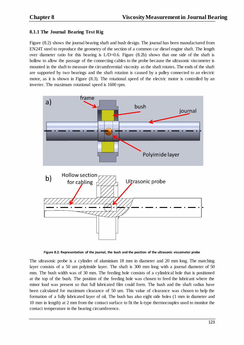
Chapter 8 Viscosity Measurement in Journal Bearing
123
8.1.1 The Journal Bearing Test Rig
Figure (8.2) shows the journal bearing shaft and bush design. The journal has been manufactured from
EN24T steel to reproduce the geometry of the section of a common car diesel engine shaft. The length
over diameter ratio for this bearing is L/D=0.6. Figure (8.2b) shows that one side of the shaft is
hollow to allow the passage of the connecting cables to the probe because the ultrasonic viscometer is
mounted in the shaft to measure the circumferential viscosity as the shaft rotates. The ends of the shaft
are supported by two bearings and the shaft rotation is caused by a pulley connected to an electric
motor, as it is shown in Figure (8.3). The rotational speed of the electric motor is controlled by an
inverter. The maximum rotational speed is 1600 rpm.
Figure 8.2: Representation of the journal, the bush and the position of the ultrasonic viscometer probe
The ultrasonic probe is a cylinder of aluminium 18 mm in diameter and 20 mm long. The matching
layer consists of a 50 um polyimide layer. The shaft is 300 mm long with a journal diameter of 50
mm. The bush width was of 30 mm. The feeding hole consists of a cylindrical hole that is positioned
at the top of the bush. The position of the feeding hole was chosen to feed the lubricant where the
minor load was present so that full lubricated film could form. The bush and the shaft radius have
been calculated for maximum clearance of 50 um. This value of clearance was chosen to help the
formation of a fully lubricated layer of oil. The bush has also eight side holes (1 mm in diameter and
10 mm in length) at 2 mm from the contact surface to fit the k-type thermocouples used to monitor the
contact temperature in the bearing circumference.

Chapter 8 Viscosity Measurement in Journal Bearing
124
The bush is contained in a frame that has the function of maintaining the journal bearing assembly
stable when rotating and to distribute the load applied. The load was applied to the bearing with a
hydraulic ram activated by an Enerpac™ pump. For this experiment the applied load varies from 0-
15kN. Figure (8.3) shows a photography of the journal bearing rig assembly.
Figure 8.3: The journal bearing test rig for viscosity measurement
8.1.2 Ultrasonic Viscometer Probe
Figure (8.4) shows schematically the ultrasonic probe. This consists of two ultrasonic PZT (PZ-5A)
bare transducers pulsing at the frequency of 5 MHz bonded on an aluminium solid line of cylindrical
shape with length of 20 mm and 18 mm in radius. At the end of the aluminium solid line, a 50 μm
thick film of polyimide is bonded to obtain a resonance frequency of 4.5 MHz.
Figure 8.4: The ultrasonic probe
Figure (8.2) shows how the ultrasonic probe is fitted in the journal. One half of the journal is hollow
to allow the passage of the cables and so the communication of the transducers with the pulsing-
receiving instrumentation. The probe is fitted and bonded in a hole of 18 mm in diameter. At first the
aluminium solid line is pushed into the hole so that the journal surface is above the aluminium line of
about 0.1 mm. At this point, the polyimide layer is bonded on the surface and the surface of the shaft

Chapter 8 Viscosity Measurement in Journal Bearing
125
is machined in a lathe so that the polyimide surface is as close as possible to the same level of the
journal surface.
8.1.3 The Slip Ring
A slip ring is needed to transfer the ultrasonic signal from the probe in the shaft to the pulsing-
receiving instrumentation outside the bearing rig. Without this component, the cables would tangle
and break apart when the shaft starts the rotation. The slip ring is a component that converts the
rotation of the shaft into a static connection with the pulser and the receiver. The slip ring used in this
experiment is shown in Figure (8.5) and is a solid-solid contact type, but also liquid-solid slip ring
exists where a conductive liquid, such as mercury, transmits the signal from the rotating part to the
static receiver. The terminations of the cables that are connected to the transducer are soldered in
correspondence of the outer copper races of the slip ring that are concentric respect to the axis of
rotation of the shaft. In this way when the journal rotates the cables inside it follow the rotation
without breaking. At the same time, while the shaft rotates, the connection from the pulsing-receiving
equipment touches the surface of the races to establish a connection to the transducers. Figure (8.6)
schematically represents the operating conditions of the slip ring.
Figure 8.5: The slip ring
Figure 8.6: Schematic representation of the slip ring

Chapter 8 Viscosity Measurement in Journal Bearing
126
8.1.4 Triggering and Data Acquisition
The ultrasonic pulsing-receiving instrumentation is the same as the one described in Chapters 6 and 7
and the data acquisition measurement chain is reported in Figure (8.7).
Figure 8.7: Ultrasonic acquisition detailed measurement chain
The main difference from the previous experimental setups is that the data are acquired from a
moving contact. The rotation was anticlockwise. An optical trigger controlled the acquisition of the
signal at the different shaft angular positions. Every time the shaft made a revolution a plastic strip
bonded on the edge of the shaft crossed the triggering sensor and a signal was acquired, as shown in
Figure (8.8). When the optical sensor was activated by passing across the plastic strip it sent a signal
that was used as trigger by a waveform generator. This waveform generator was another TTI TG5011
type and its task was to pulse a single cycle square pulse every time it was triggered. This pulse was
used by a second waveform generator as an external trigger to fire the chirp signal. To acquire signals
at position other than the crossing point, a time delay was added to the square signal produce by the
first signal generator. A LabView™ program controlled the oscilloscope to obtain a signal that was
average of 500 acquisitions.
Figure 8.8: Signal acquisition by incremental delays

Chapter 8 Viscosity Measurement in Journal Bearing
127
8.1.5 Reflection Coefficient Acquisition in Journal Bearings
The acquisition of the reflection coefficient in journal bearings is complicated by the absence of an air
reference interface. The solid-air boundary was used as convenient reference interface in Chapters 6
and 7 to conduct the reflectance experiments. This is not possible in the experiment involving the
journal bearing. The chirp technique proposed in section (7.2) can be used to overcome this limitation.
In chapter 7, it was shown that the portion of the chirp that contains the resonance frequency
component attenuates massively, while the portion of the chirp with frequency components outside
resonance does not attenuate. This means that the part of the signal that attenuates because of the
resonance can be used as measurement, while the component outside resonance acts like the case of
solid-air interface, thus being an ideal reference without need for using any air interface. Figure (8.9)
shows schematically how this novel measurement technique works by referring to Figure (7.10).
Figure 8.9: It is possible to use the chirp technique to acquire reflection coefficients in journal bearing without using the common air reference because the frequencies outside the resonance frequencies are not sensitive to the fluid
The usual equation to measure the reflection coefficient (
) cannot, however, be used in this
case. As it is shown in Figure (8.9), when only the air is in contact with the matching layer probe the
amplitude of the frequency component associated with resonance is (100 mV). This is different from
the amplitude of the frequency components outside resonance (200 mV). As a consequence, before a
comparison between the different frequency components is possible, the amplitude of the frequency
components at resonance and outside resonance has to be the same when no liquid is in contact. In
this way, the drop in amplitude at the resonance frequency when the liquid is in contact with the probe
can be compared with the response of the frequency component that is not sensitive to the presence of
the fluid. A calibration of the frequency response at resonance and outside resonance is needed and
the reflection coefficient can be calculated as:

Chapter 8 Viscosity Measurement in Journal Bearing
128
(8.1)
The weight w(T) in equation (8.1) is a function of temperature. In fact, the transducer characteristic
varies with the temperature and the ratio between the frequency components at different temperature
may vary as well. To obtain the weight in equation (8.1) the shaft is put in an oven and the amplitude
variation of the component at 4.5 MHz (resonance) and 9 MHz (frequency outside resonance chosen
as reference) is recorded and averaged for three heating and cooling cycles. The amplitudes of the
signals obtained are then divided to obtain the weight curve. Figure (8.10) shows the characteristic
temperature curve and the weight function for this particular case.
Figure 8.10: Weight function for the novel reflectance acquisition technique
8.2 Experimental Protocol
Table (8.1) reports the experiment matrix. Five engine lubricants with different compositions were
tested at the rotational speed of 500 rpm and 1000 rpm and at different load levels. The load was
chosen to obtain a significant variation in viscosity due to the pressure variation. Every experiment
run was repeated twice in a row with a pause of one hour between each test run to disperse the heat
accumulated in the shaft and bush during the previous experiment. Every time a new sample was
tested the rig was cleaned by flushing the new test lubricant until only the new sample was present in
the contact area. The results for the high detergent were affected by grip and the results from this
experiment are analysed separately in section 8.2.2.
Sample Load at 500 rpm (kN) Load at 1000 rpm (kN) Ester 12 12
PAO40 15 20 VM1 12 15
VM2 12 15 High Detergent 15 15
Table 8.1: Experimental test matrix: load for every sample at different rotational speed.

Chapter 8 Viscosity Measurement in Journal Bearing
129
8.3 Results
Figures (8.11-8.14) show the viscosity results acquired from the experimental apparatus described in
sections (8.1-8.2) in the form of angle-viscosity graphs. The shape of the viscosity curves is very
similar for all the oils tested. It can be noticed that where only the temperature effects are important
the viscosity is lower, while the effect of the load at around 160 degrees causes the viscosity to rise to
its maximum.
Figure 8.11: Angle-Viscosity results for the oil VM1 for two bearing rotational speed

Chapter 8 Viscosity Measurement in Journal Bearing
130
Figure 8.12: Angle-Viscosity results for the oil VM2 for two bearing rotational speed
Figure 8.13 Angle-Viscosity results for the oil Pao40 for two bearing rotational speed

Chapter 8 Viscosity Measurement in Journal Bearing
131
Figure 8.14 Angle-Viscosity results for the oil Ester for two bearing rotational speed
The values of temperature in Figures (8.11-8.14) refer to the average temperature measured in the
different zones. Figure (8.15) shows the five viscosity regions with respect to the bearing geometry in
a simplified sketch.
Figure 8.15: The five viscosity regions highlighted by the bearing experiment

Chapter 8 Viscosity Measurement in Journal Bearing
132
Region 1 has low temperature and low load and is associated with the inlet region. The oil is
fed at the angle of 30 degrees at room temperature and the viscosity value measured is very
close to that measured in section (7.5) when no pressure or temperature gradient is applied.
Region 2 the temperature rises and the load is still low. This region is characterized by a
lower value of viscosity because the temperature rises and the load value is negligible.
Attention is drawn to the measured value of temperature, which is much higher than in region
1 and so the viscosity drops because this is the last region for which viscosity is measured. In
fact, the viscosity is measured anticlockwise and this means that after region 1 the first value
of viscosity is measured in Region 5.
Region 3 is characterized by a temperature rise and high load. The viscosity value measured
in this region is higher than the inlet value of viscosity, and this is due to the fact that the
viscosity loss due to the increment in temperature is balanced by the viscosity increment due
to higher pressure, as explained in Figure (8.16).
Figure 8.16 Schematic representation of the viscosity profile in the region under maximum load
Region 4 is characterized by high temperature and low load. This region is characterized by a
drop in viscosity and it is also the area where minimum film thickness is expected. It is
interesting to notice that the viscosity profile in this region is similar to the one in region 2.
This is due to the fact that the temperature measured in region 4 is very close to the one
measure in region 2. In region 4, therefore, the temperature effect is the dominant one even if
a residual load effect is present, but this is not enough to rise considerably the viscosity that
is, in fact, very similar to the one measured in the unloaded region 2.
Region 5 is characterized by a lower contact temperature, influenced by the inlet oil
temperature, and there is no load. It can be noticed that the viscosity value in this case is
higher than in region 4, but slightly lower than in region 1 this is because the oil inlet
temperature influence the contact temperature and so the overall value of viscosity in this
region. These results can be analysed in terms of viscosity measured in the different areas as
reported in table (8.2).

Chapter 8 Viscosity Measurement in Journal Bearing
133
VM1 (mPas) VM2 (mPas) PAO40 (mPas) Ester (mPas) 1000 rpm 500 rpm 1000 rpm 500 rpm 1000 rpm 500 rpm 1000 rpm 500 rpm
Region 1 35 35 170 180 350 400 160 160 Region 2 25 25 100 120 230 300 120 140
Region 3 40 45 170 180 400 450 170 180
Region 4 18 20 110 120 180 200 100 120 Region 5 25 25 120 130 250 260 120 130
Table 8.2: Average viscosity value for the 5 viscosity regions in the results in Figure (8.11-8.14)
This table shows that the average oil viscosity is substantially constant in regions 1 to 3, but in drops
dramatically in region 4 where the maximum temperature and the minimum load are encountered. The
results presented in this table are presented as a graph in Figure (8.17).
Figure 8.17: Comparison of average viscosity in the different load-temperature regions that are present in the journal bearing
8.3.1 Effect of Seizure
The experiment involving the high detergent sample was affected by grip due to failure in aligning the
load correctly and the results are analysed in this section. Figure (8.18) reports the effect of the solid-
solid adhesion contact between the bush and the journal. The adhesion led the motor to grip while
trying to make the journal rotating.
The result of this adhesion was such a high increment in temperature due to friction that the thermal
effect overcame the effect of the applied load. Figure (8.19) shows the angle-viscosity results for the
high detergent sample.
In Figure (8.19) it can be noticed that the viscosity decreases constantly even in the maximum load
region. This happens because the high increment in temperature is dominant over the expected
increment in viscosity due to the rise in pressure.

Chapter 8 Viscosity Measurement in Journal Bearing
134
Figure 8.18: Brass adhesion to the journal for the high detergent sample
Figure 8.19: Angle-viscosity results for a high detergent sample. The results are influenced by grip.

Chapter 8 Viscosity Measurement in Journal Bearing
135
8.4 Analytical Simulation of Journal Bearing Viscosity Field
The performances of the journal bearing set-up are simulated and compared with a semi-isoviscous
solution of the hydrodynamic Reynolds equation for journal bearings. The model does not take into
account bearing vibration, elastic deformation or deflection and shear heating, and it calculates the
pressure field in the journal bearing with the assumption that the viscosity does not change around the
bearing circumference (isoviscous). The viscosity is chosen at the so called effective temperature
( ). This is the average temperature at which the journal bearing is operating. The model is
implemented in Matlab™ using the finite differences technique (Stachowiack and Batchelor, 2001)
and Figure (8.20) reports the scheme of how the model is implemented.
Figure 8.20: Flow chart of the numerical model implemented to simulate the bearing pressure field
The semi-isoviscous model was chosen because the non-isoviscous solution requires the knowledge
of more input parameters that are difficult to measure or for which information are limited. These
parameters are, for example, the variation of the oil density with temperature and the thermal
conductivity. The input eccentricity parameter was obtained through the Raimondi-Boyd (1958) chart
that correlates the non-dimensional load with the eccentricity. Figure (8.21) reports the chart. In
Figure (8.21) the non-dimensional load is a parameter that correlate the absolute load applied to the
bearing to the viscosity the L/D ratio and the bearing clearance. The intersection of with the L/D
curves gives the desired value of eccentricity.
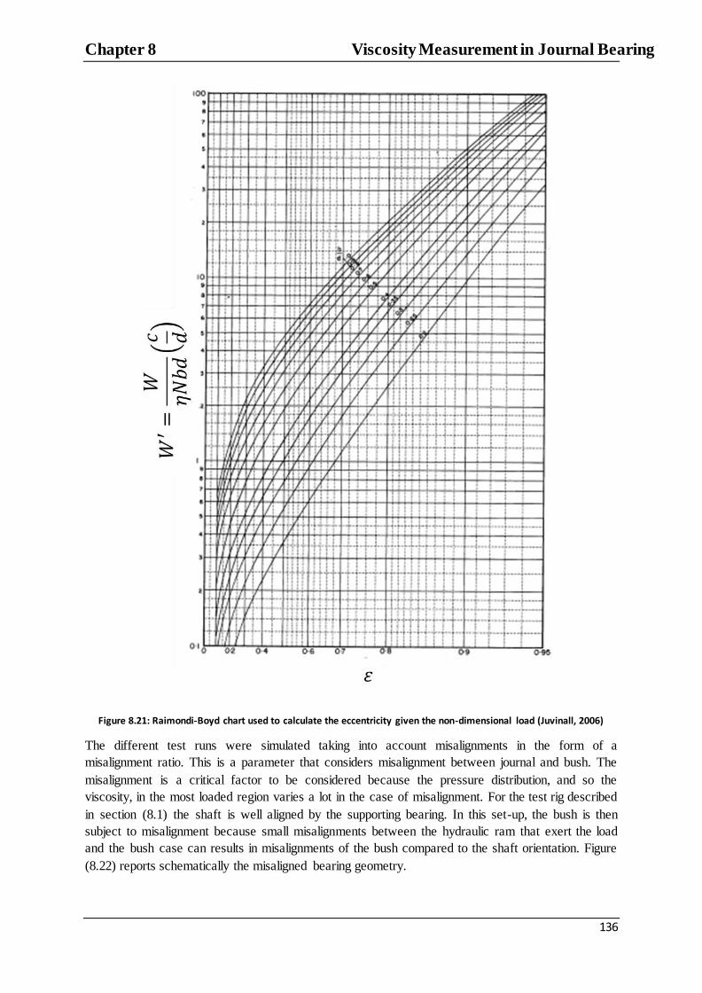
Chapter 8 Viscosity Measurement in Journal Bearing
136
Figure 8.21: Raimondi-Boyd chart used to calculate the eccentricity given the non-dimensional load (Juvinall, 2006)
The different test runs were simulated taking into account misalignments in the form of a
misalignment ratio. This is a parameter that considers misalignment between journal and bush. The
misalignment is a critical factor to be considered because the pressure distribution, and so the
viscosity, in the most loaded region varies a lot in the case of misalignment. For the test rig described
in section (8.1) the shaft is well aligned by the supporting bearing. In this set-up, the bush is then
subject to misalignment because small misalignments between the hydraulic ram that exert the load
and the bush case can results in misalignments of the bush compared to the shaft orientation. Figure
(8.22) reports schematically the misaligned bearing geometry.

Chapter 8 Viscosity Measurement in Journal Bearing
137
Figure 8.22: Misaligned load applied to the bush and misalignment angle
In this figure (8.22) the misaligned load W causes the bush to be deflected of an angle α. The input
parameters for the numerical model and the values of eccentricity are reported in table (8.3) for all the
samples.
Parameter Ester PAO40 VM1 VM2 High Detergent 140 250 25 100 50
1.7109 0.9125 7.984 1.597 4.79 3.43 1.372 16 2.134 6.403
𝜀 0.425 0.29 0.72 0.4 0.62 𝜀 0.58 0.39 0.82 0.45 0.68
0.1168 0.0591 0.642 0.1026 0.3298
0.261 0.0977 1.543 0.1315 0.4828
Misalignment ratio 0.5 0.5 0.5 0.5 0.5
Table 8.3: Entry parameters of the analytical model
In table 8.3 the inlet viscosity is measured with the ultrasonic viscometer, is the non-dimensional
load, 𝜀 is the eccentricity obtained from Figure (8.21), and is the non-dimensional maximum
pressure obtained by running the analytical model for the different samples, where the non-
dimensional pressure is calculated as
. The misalignment ratio is set to 0.5 to take into
account of unavoidable position misalignments of the hydraulic ram with respect to the axis of
rotation of the bearing in the journal bearing test rig. This misalignment was the primary cause of
seizure for the experiment reported in section 8.3.1. The program calculates parameters the friction
coefficient, the maximum load capacity of the bearing and the pressure field. The pressure field is the
output parameter of interest in this analysis. This is calculated in the case of no misalignment or in
case the misalignment ratio is variable. Figure (8.23a, b, c) report an example of the three dimensional
pressure field calculated for a lubricant with no misalignment (Figure 8.23a), with a small
misalignment ratio (Figure 8.23b) and with a high misalignment ratio (Figure 8.23c).

Chapter 8 Viscosity Measurement in Journal Bearing
138
Figure 8.23 a) Aligned journal bearing, b) Misalignment ratio 0.1, c) Misalignment ratio 0.5
Only the values of pressure from the centre load line are used to obtain viscosity because the
ultrasonic probe acquires data from those positions. Figures (8.24-8.27) show the journal bearing
pressure distributions for the different oils samples. These results are obtained at the input conditions
reported in Table (8.3).
Figure 8.24: Pressure distribution PAO 40 sample

Chapter 8 Viscosity Measurement in Journal Bearing
139
Figure 8.25: Pressure distribution Ester sample
Figure 8.26: Pressure distribution VM1 sample
Figure 8.27: Pressure distribution VM2 sample

Chapter 8 Viscosity Measurement in Journal Bearing
140
The pressure fields are converted in viscosity using the Barus equation implemented with the
pressure-viscosity coefficients calculated in section (7.5) and here reported in table (8.4).
Sample Pressure-viscosity coefficient ( ) Ester 21.1 Pao40 27.5
VM1 17.8 VM2 25.1
Table 8.4: Pressure-viscosity coefficients
The pressure-viscosity coefficients are assumed to be constant thought the variation in temperature
experienced in the experiments. Figures (8.18) to (8.21) compare the results of the ultrasonic
viscometer with the results from the isoviscous model.
Figure 8.28: Comparison of analytical and experimental results for the sample Ester
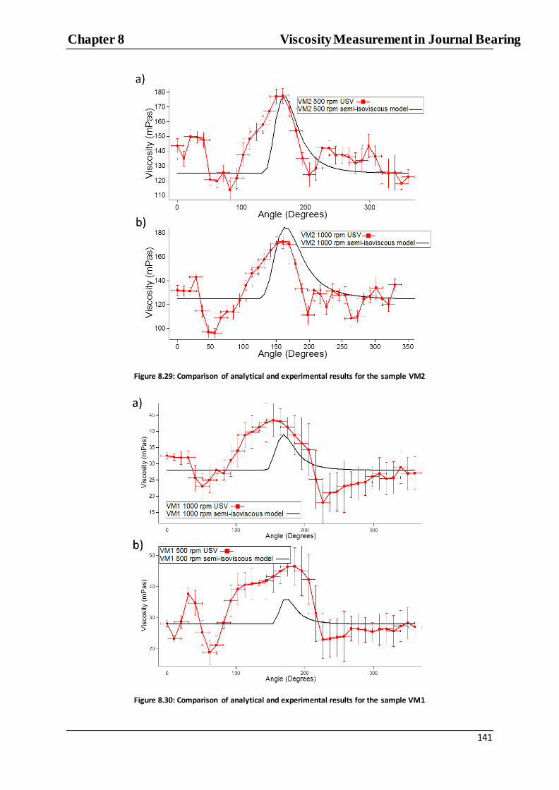
Chapter 8 Viscosity Measurement in Journal Bearing
141
Figure 8.29: Comparison of analytical and experimental results for the sample VM2
Figure 8.30: Comparison of analytical and experimental results for the sample VM1

Chapter 8 Viscosity Measurement in Journal Bearing
142
Figure 8.31: Comparison of analytical and experimental results for the sample PAO40
The results show that the ultrasonic viscometer identifies the angle at which maximum pressure
occurs and the maximum loaded region where the viscosity increases. The isoviscous model does not
calculate the variation of temperature and viscosity in the regions that are not loaded. This brings to a
substantial difference in the viscosity measured outside the loaded region. Figure (8.31) shows that
the simulation for the VM1 sample is not precise as the other samples tested. This is due to the fact
that the input parameters for this sample are related to the base oil properties and not to the parameters
for the polymer lubricant.
8.4.1 Power Losses
The viscosity results are important because they can be used to calculate the frictional power losses at
each position in the journal bearing circumference. Figure (8.32) shows the geometry of the bearing as
an infinitesimal lubricant quantity is sheared at the contact interface. For this geometry the localized
power losses are:
𝜏 𝜔 (8.2) where 𝜏 is the shear force on the element of surface area A and 𝜔 is the entraining velocity.
This expression can be expanded in terms of the frictional parameters such as viscosity and film
thickness as:
𝜔
(8.3)
where is the surface area and dy is the film thickness at every bearing location. Assuming a
linear velocity gradient
and it follows:

Chapter 8 Viscosity Measurement in Journal Bearing
143
𝜔
𝜔
(8.4)
Figure 8.32: Scheme of the journal bearing geometry
Consequently:
𝜔 ∫
(8.5)
In section 8.3 the viscosity results were acquired at discrete locations. Because of this, the integral in
equation (8.5) becomes the sum of
at each discrete locations and becomes
where i is the
number of discrete points acquired. Therefore, equation (8.5) becomes:
𝜔 ∑
(8.6)
where the film thickness is calculated from the Raimondi-Boyd (1958) charts as:
𝜀 𝜃 (8.7) Figure (8.33 a, b) shows the localized power loss at each location that are calculated using equation
(8.6) and the viscosity results in Figure (8.28)-(8.31), while Figure (8.33 c, d) shows the total power
losses obtained cumulatively at each location by integration of the curves in Figure (8.33 a, b). The
total power losses are compared with the Petroff (Juvinall, 2006) equation for the total power losses in
a plain journal bearing:
𝜔
(8.8)
where is the Petroff total power loss in a plain journal bearing.
It can be noticed that the majority of the power losses are encountered in the bearing region where the
higher viscosity and the minimum film thickness are present. From equation (8.6), when the viscosity
is high and the film thickness is low the total power rises at its maximum. Figure (8.34) shows on a
polar graph the power losses versus angle for the Ester oil at 500 rpm with respect to the bearing
geometry. The graph shows clearly that the majority of the power losses are concentrated in the small
area where the film thickness is the minimum. The ultrasonic viscometry technique described in this
chapter can then be applied to the design of real bearing where the losses due to friction have to be
minimized.
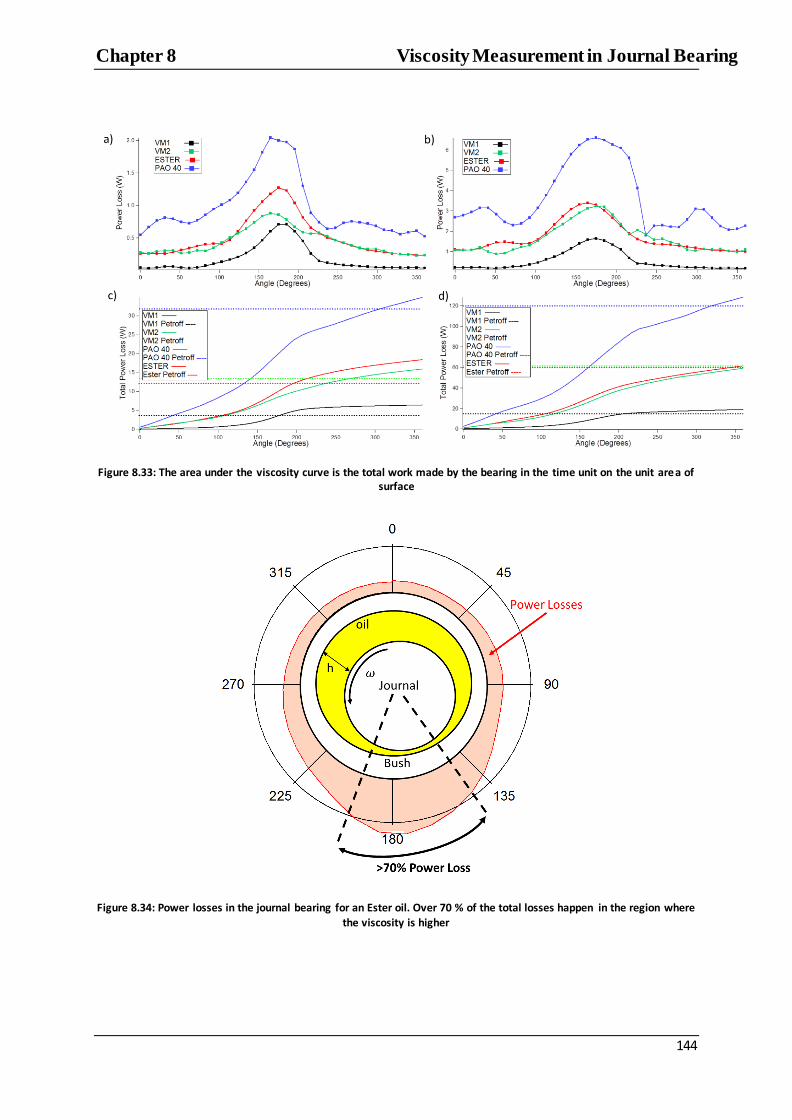
Chapter 8 Viscosity Measurement in Journal Bearing
144
Figure 8.33: The area under the viscosity curve is the total work made by the bearing in the time unit on the unit area of surface
Figure 8.34: Power losses in the journal bearing for an Ester oil. Over 70 % of the total losses happen in the region where the viscosity is higher

Chapter 8 Viscosity Measurement in Journal Bearing
145
8.5 Preliminary Application to a Real Bearing
The matching layer technique proved to be very effective for an aluminium-polyimide setup.
However, in real engine applications polyimide cannot be used as matching layer for long test run
because the layer would wear out. To overcome this limitation it is possible to use the existing coating
that are found, for example in shell bearing, as matching layer. Babbit and Iron-Oxide (Irox ®
bearings) are the most used coating material in automotive steel engine bearing. Iron oxide, in
particular, is proven to be a high performance coating. This is a polymer with high alumina content
therefore the acoustical impedance of this material is very close to that of aluminium. From Figure
(7.5) it can be noticed that steel and aluminium are matched and it is possible to expect a reflection
coefficient of around 0.8 for a lubricant of 250 mPas in viscosity. The coating layer thickness is
around 30-50 micrometre and from equation (7.2) it is expected a resonant frequency between 4 and 5
MHz. It is then possible to bond an ultrasonic shear transducer directly in contact with the steel shell
to use the steel-iron oxide line as it is done for the aluminium-polyimide in chapter 7 and in chapter
(8.1 to 8.4). Figure (8.35) shows an ultrasonic viscometer setup for in-situ applications in a shell
bearing lubrication analysis.
Figure 8.35: Ultrasonic viscometer setup in a coated shell partial bearing
The setup is tested exactly as the one described in chapter (7) using a four cannon viscosity standard
mineral oil. Table (8.6) reports the characteristic of the oil tested.
Oil Sample Viscosity (mPas) @25°C S20 29.1 N35 55.9
S60 98.5
N100 200.7
Table 8.6: The mineral oils tested to calibrate the ultrasonic viscometer on the partial shell bearing
Similarly as in section (7), the reflection coefficient is acquired from the mineral oil and is plotted
against the viscosity, as shown in Figure (8.36)

Chapter 8 Viscosity Measurement in Journal Bearing
146
Figure 8.36: Calibration curve for the shell bearing ultrasound viscometer
The viscosity-reflection coefficient experimental points are interpolated with a logarithmic function as
it was done in chapter (7) and it is was observed that the reflection coefficient at 200 mPas is around
0.87, as it is expected by the theory and the model described in sections (7.1). It is also noticed that
the correlation coefficient R is less accurate than the correlation coefficient found in chapter (7). This
is due to the fact that as the steel-iron oxide combination is not a perfect match and the sensitive to the
measurement does not increase as much as in the aluminium-polyimide case. Nevertheless, the setup
described in this section proves to be sensitive enough to discriminate the viscosity of the calibrated
oil in a wide range and with a good sensitivity.
8.6 Conclusions
This chapter illustrated the application of the matching layer technique to a journal bearing test rig.
Four lubricants were tested: two base synthetic oils and two oils with viscosity modifiers functions.
The ultrasonic viscometer was mounted in the journal to allow measurement of the circumferential
viscosity at different rotational speed and different loads. The experimental results were compared
with a simulation of the Reynolds equation for journal bearings hydrodynamic lubrication. The
simulation was conducted with a finite difference numerical algorithm. The comparison of the results
shows that the ultrasonic viscometer and the model identify the same loaded region and the same
angle at which the maximum load occurs. The discrepancies between the maximum viscosity
measured with the numerical model and the viscometer is found in the fact that the numerical model is
ideal, thus not taking into account vibration, elastic deflection, solid-solid contact, thermal effect and
shear heating. Overall, the ultrasonic viscometer proves to be a useful tool for in-situ investigation of
journal bearing, and potentially a variety of engine components. The experimental results showed that
the isoviscous model is not sufficient to design a journal bearing as the viscosity losses due to the
thermal effect varied from 25% for the thin oils to 60% for the thickest samples tested. The method
was also preliminary tested on a real iron-oxide coated journal bearing. The results of the viscometer
calibration on this component are in line with the expected theoretical model presented in chapter 7.1,
thus validating this sensing technique as applicable in real engines components.

Chapter 9 Conclusions
147
Chapter 9 Conclusions
Conclusions
This chapter presents a summary of the findings of this research. The area of work analysed are: a
novel ultrasonic mathematical model for the analysis of Non-Newtonian fluids, the development of
the matching layer technique as a novel sensing technique to measure viscosity and the application of
this technique to a journal bearing.
9.1 The Ultrasonic Model for Non-Newtonian Fluids The first goal of this work was to enhance the existing ultrasonic model to the analysis of fluid
viscosity from a Newtonian to a Non-Newtonian (or generalized Newtonian) model. To do so the
simplest viscoelastic model, the Maxwell model, is implemented to correlate viscosity and reflection
coefficient. The application of this model to the common reflectance setup demonstrated that this
model is ideal to study high viscosity lubricants (viscosity >0.3 Pas). The application of this model to
the quarter wavelength matching layer technique demonstrated, through the increment in sensitivity in
the measurement technique, that this model is ideal to study also low viscosity fluids. The application
of this model allowed the implementation of an empirical model that correlates viscosity to the
reflection coefficient only to make oil measurements also in the situation where accurate reference or
the material properties are not known.
The results presented in section 7.4 shows also that the viscoelastic model is necessary to analyse
lubricants under pressure and so to analyse real engine components. It is shown in fact that when the
lubricant is under pressure the loss modulus increase exponentially and so the behaviour of the oil
tends to be highly non-Newtonian.
9.2 The Quarter Wavelength Matching Layer Sensing Technique The common reflectance cannot be used to the analysis of engine lubricant in-situ because of the high
acoustical mismatch between the solid engine component material (usually steel) and the oil, as
shown in chapter 6. The acoustic mismatch is overcome by the implementation of a quarter
wavelength matching layer technique. This consists in interleaving between the solid and the oil a
layer of material that allows a better sound transmission and increase the sensitivity of the
measurement. The sensing technique was first tested on an aluminium-polyimide system. The probe
was tested at different shear rates, temperature, and pressure.
The shear rate experiment confirmed that at high ultrasonic frequencies the Cox-Merz rule (Cox and
Merz, 1958) is no longer valid, and that only the base of the oil is sheared while additives, polymer
and particle with high inertia do not contribute to the ultrasound viscometer reading. These results are
in line with the experiments conducted by Bair (2007). The experiment showed that sweeping
ultrasonic frequencies different shear rate at interface are excited and the transition from first
Newtonian plateau to the second Newtonian plateau is highlighted.
The experiment with temperature vitiation aimed to analyse the behaviour of the matching layer as the
temperature is highlighted. The experiment showed that an increment in temperature shifted slightly
the resonance frequency because the bonding between the matching layer and the solid kept on curing
with the temperature cycle. This behaviour can be controlled by directly coating the matching layer on
the solid surface.
Chapter 9 Conclusions
148
The pressure experiment was needed to analyse the performance of the matching layer technique at
the journal bearing operating pressures. The experiment demonstrated that only the base of the oil is
analysed because the pressure viscosity coefficient is the one expected for synthetic oil. The results
were also converted in relaxation time and complex shear modulus. These results highlighted that as
the pressure increases the term G‟ takes over the term G‟‟, thus meaning that the Non-Newtonian
behaviour is accentuated and that a viscoelastic model is needed to test in auto engines.
9.3 Application of the Matching Layer Method in a Journal Bearing The quarter wavelength matching layer technique is finally applied to a journal bearing. The
ultrasonic viscometer is mounted on a journal to measure the circumferential viscosity in the bearing.
This is the first non-invasive circumferential viscosity measurement in a journal bearing. The
viscosity-angle results were compared with the analytical results from a numerical model of the
Reynolds equation implemented with the finite differences technique. The results show that both the
ultrasonic viscometer and the numerical solution identify the same angle at which the maximum
pressure occur and the loaded region contact area. The discrepancies between the actual results and
the model are to be identified in the simplifications of the model that does not consider crucial factors
such as vibration, deformation and shear heating at the contact surface.
Finally, the ultrasonic viscometer setup was developed for a real diesel engine shell bearing. In this
case the matching layer was the coating of the steel shell. Steel and iron-oxide coating (aluminium
like acoustical impedance) is a match, as shown from the theory in section 7.1. The calibration
reflection coefficient-viscosity plot was made in the same way as for the aluminium-polyimide
ultrasonic probe. The results show that the same logarithmic empirical law applies to this case and
that, even if the sensitivity is slightly lower than the aluminium-polyimide case, the matching layer
technique can be applied in case of a real component is instrumented.
9.4 Future Directions The following is a list of future development for this research:
Implement a broadband ultrasonic viscometer to analyse oils at frequencies ranging from
kHz to GHz to identify the shear rate transition zone between the first and the second
Newtonian plateau. The current work focused on the frequency range 1-10 MHz. In future, it
will be of great interest to obtain viscosity readings at kHz frequencies for a comparison with
conventional rheometers and at frequencies in the magnitude order of Hz because of the
lack of knowledge in the lubricant behaviour at such high frequencies.
Use the results to enhance the current viscoelastic models for Non-Newtonian fluid analysis.
The mathematical model developed in Chapter 5 is based on the Maxwell model. This is a
relaxation time based algorithm. In future it will be of great interest to develop more complex
model that could take into account of the specific chemical behaviour of the tested lubricant
sample.
Instrument the ultrasonic viscometer technique in a real engine to enhance current testing
techniques protocols. The matching layer viscometer shows the potential to be mounted in
engine test rigs to study lubricant performances in journal bearings (plain or partial), but also
in other coated components (e.g. piston oil linen) and in oil swamps for in-situ and real time
analysis. This is of crucial interest for chemical and manufacturing companies that are trying
to enhance oils and engine design to respect the international fuel economy regulations.
Use this technique to test performances of coatings and lubricants. The use of a wide range of
frequencies would allow following the evolution of the base oil and the additive separately

Chapter 9 Conclusions
149
and this would be of great benefit for designing of effective lubricants for different engine
operating situations.
Implement the matching layer technique for the analysis of EHL (elastohydrodynamic
lubrication) contacts. This is of primary interest in the field of tribology. It is still not
completely clear what are the mechanisms that govern the lubrication in components
subjected to EHL contacts, such as ball bearings. The implementation of this novel ultrasonic
technique in these components would open up to a better understanding of EHL.
Application of the matching layer technique to other disciplines such as biomedical
engineering. The matching layer method, in fact, could be used to develop novel, non-
invasive instruments for the remote monitoring of bio-fluids properties. Bio-fluids (e.g
blood) viscosity is directly linked to conditions and disease in the human body. For instance
the presence of a virus in the blood stream would change its viscosity. Miniaturized
ultrasonic probes manufactured on the same principles of the one described in Chapter 7
could be used to obtain important information on the conditions of bio-fluids remotely and
non-invasively with great benefits for the patients and the health services.

150
References
Achenbach J.D. (1973) Wave propagation in elastic solids, 1st ed. North Holland Publishing Company
Ahlberg L.A. and Cohen-Tenoudji F. (1988) High temperature ultrasonic viscometer. US Patent
Number 4779452
Alford L.P. (1911) Bearings and their lubrication, 1st ed., Mc Graw Hill
Al-Hadithi T.S.R et al. (1992) The relationship between the linear (oscillatory) and nonlinear (steady-state) flow properties of a series of polymer and colloidal systems. Colloid and Polymer
Science, Vol.270 pp.40-46.
Alvarez-Arenas T.E.G. (2004) Acoustic impedance matching of piezoelectric transducers to the air.
IEEE Transactions on Ultrasonics, Ferroelectrics and Frequency Control. Vol. 51(5) pp.624-633
Arora, A. (2005). Text Book of Inorganic Chemistry. Discovery Publishing House.
Augenstein et al. (1999) Method and apparatus for determining the viscosity of a fluid in a container.
US Patent Number CA2258329
Bair, S,. (2007). High pressure rheology for quantitative elastohydrodynamics (Vol. 54). Elsevier.
Bair, S., Liu, Y., Krupka, I., et al., (2008): The shear-thinning elastohydrodynamic film thickness of a
two-component mixture., Journal of Tribology, 130(2), 021502
Bair, S., Vergne, P., Querry, M.,(2005) A unified shear-thinning treatment of both film thickness and
traction in EHD., Tribology Letters, 18(2), 145-152
Bair S., Yamaguchi T. et al.(2014) Oscillatory and steady shear viscosity: The Cox-Merz rule
superposition and application to EHL friction. Tribology International Vol.79 pp. 126-131
Bair S. and Winer W.O., (1980) Some observations on the relationship between lubricant mechanical
and dielectric transitions under pressure, Trans. ASME, Journal of Lubrication Tech., 102, 2, pp 229-
235
Barlow A.J. and Lamb J. (1959) The visco-elastic behaviour of lubricating oils under cyclic shearing
stress. Proc. R. Soc. Lond. Vol 253 pp. 52-69
Barus C. (1893). Isotherms, isopiestics and isometrics relative to viscosity. American Journal of
Science. Vol. 45 pp. 87-96
Benasciutti D., Munteanu M.G. and Flumian F. (2012) A numerical approach for static and dynamic analysis of deformable journal bearings. World Academy of Science, Engineering and Technology .
Vol.6, pp. 609-620
Buckin V. and Kudryashov E. (2001) Ultrasonic shear wave rheology of weak particle gels. Adv.
Colloid Interface Sci. Vol. 89-90 pp. 401-422
Buiochi F., Higuti R.T. and Furukawa C.M. (2000) Ultrasonic measurement of viscosity of liquids,
IEEE Ultrasonics Symposium. Vol. 1 pp. 525-528
151
Bujard M.R. (1989) Method of measuring the dynamic viscosity of a viscous fluid utilizing acoustic
transducer. US Patent Number 04862384
Cameron A. (1966) Priciples of lubrication. 1st ed, Longmans Green and Co. Ltd
Cameron A. (1981). Basic lubrication theory , 1st ed., Ellis Horwood Limited
Carreau P.J. (1972) Rheological equations from molecular network theories. Transactions of the
Society of Rheology Vol. 16(1) pp. 99-127
Collin R.E. (1955) Theory and design of wide-band multisection quarter-wave transformers.
Proceedings of the IRE Vol.36 pp. 621-629
Covitch, M. J., & Trickett, K. J. (2015). How Polymers Behave as Viscosity Index Improvers in
Lubricating Oils. Advances in Chemical Engineering and Science, 5(02), 134.
Cox W.P and Merz E.H. (1958) Correlation of dynamic and steady flow viscosities. J Polym Sci
Vol.28(118) pp.619–22.
Crouch R.F. and Cameron A. (1961) Viscosity-temperature equations for lubricants. Journal of the
Institute of Petroleu. Vol, 47 pp. 307-313
Curie J, Curie P. (1880) Sur l‟électricité polaire dans les cristaux hémièdres à faces inclinées. C R
Acad Sci Vol.91 pp.383–386
Dabir S. et al. (2010) Viscosity of liquids: theory, estimation, experiment and data . 2nd
Ed., Springer.
Dean E.W. and Davis G.H.B (1929). Viscosity variations of oils with temperature. Chem. and Met.
Eng. Vol. 36 pp. 618-619
Desilets C.S. et al. (1978) The design of efficient broad-band piezoelectric transducers. IEEE
Transactions on Sonics and Ultrasonics. Vol. 25(3) pp.115-125
Dukhin A.S. and Goetz P.J. (2009) Bulk viscosity and compressibility measurement using acoustic
spectroscopy. The Journal of Chemical Physics. Vol.130
Dwyer-Joyce R.S. and Kasolang S. (2008) Viscosity measurement in thin ubricant films using shear
ultrasonic reflection. Proceeding of the Institution of Mechanical Engineers, Part J: Journal of
Engineering Tribology. Vol. 222 (3) pp. 423-429
Emmert S.W. (1986) Apparatus and method for determining the viscosity of a fluid sample. US
Patent Number 4721874
Farone W.A. et al. (2002) Acoustic viscometer and method of determining kinematic viscosity and
intrinsic viscosity by propagation of shear waves. US Patent Number 6439034
An F., and Sauer, A. (2004) Comparison of passenger vehicle fuel economy and GHG emission
standards around the world. Pew Center on Global Climate Change
152
Firestone F.A., (1940) Flaw detecting device and measuring instrument, US Patent Number 2280226A
Franco E.E. and Adamowski J.C. (2008) Viscosity measurement of Newtonian liquids using the
complex reflection coefficient. IEEE Transactions on Ultrasonics, Ferroelectrics, and Frequency
Control. Vol. 55 (10) pp. 2247-2253
Franco E.E., Adamowski J.C. and Buiochi F. (2010)Ultrasonic viscosity measurement using the shear
wave reflection coefficient with a novel signal processing technique. IEEE transactions on ultrasonics,
ferroelectrics, and frequency control . Vol. 57(5) pp.1133-1139.
Greenwood J.A. and Williamson J.B.P. (1966) Contact of nominally flat surfaces. Proc. R. Soc. Lond.
Vol. 295 pp. 300-319
Greenwood M.S. (2003) Self calibrating apparatus and method for ultrasonic determination of fluid
properties. US Patent Number CA2479119
Greenwood M.S. and Bamberger J.A. (2002) Measurement of viscosity and shear wave velocity of a
liquid or slurry for on-line process control. Ultrasonics Vol. 39 pp 623-630
Haller M.I. and Khuri-Yakub B.T. (1992) 1-3 air composite for ultrasonic air transducers. Ultrasonic
Symposium pp. 937-939
Hamrock B.J. and Dowson D. (1981) Ball bearing lubrication, the elastohydrodynamic of elliptical
contacts. 1st ed, John Willey&Sons.
Hinrichs R.J. (1985) Method for determining resin viscosity with ultrasonic waves. US Patent
Number 4559810
Hutton, J.F. (1967) Viscoelastic relaxation spectra of lubricating oils and their component fractions.
Proc. Roy. Soc. London Mathematical and Physical Sciences. Vol. 304, 1476, pp.65-80
Irving, J.B. and Barlow, A.J. (1971) An Automatic High Pressure Viscometer, J. Phys. E., Vol. 4, No.
3, pp. 232–236
Johnson, K. L., & Tevaarwerk, J. L. (1977). Shear behaviour of elastohydrodynamic oil
films. Proceedings of the Royal Society of London A: Mathematical, Physical and Engineering
Sciences Vol. 356, No. 1685, pp. 215-236
Ju H., Gottlieb E.J. and Augenstein D.R. et al. (2010) An empirical method to estimate the viscosity
of mineral oil by means of ultrasonic attenuation. IEEE Tras. Ultrason. Ferroelectr. Freq. Control.,
Vol 57(7) pp. 1612-1620
Juvinall R.C. and Kurt M.M. (2006) Fundamentals of machine component design. 5th
ed., John
Wiley&Sons
Kaatze U. and Behrends R. (2001) A high frequency shear wave impedance spectrometer for low
viscosity liquids. Measurement Sciece and Technology. Vol 12(4)
Kauzlarich J.J. (1996) Electronic viscometer, US Patent Number 5571952

153
Kim J.O. and Bau H.H. (1988) Instrument for simultaneous measurement of density and viscosity,
Rev. Sci. Instrum. Vol 60 pp. 1111-1115
Kinsler, L. E., Frey, A. R., Coppens, A. B., & Sanders, J. V. (1999). Fundamentals of acoustics.
Fundamentals of Acoustics, 4th Edition, by Lawrence E. Kinsler, Austin R. Frey, Alan B. Coppens,
James V. Sanders, pp. 560. ISBN 0-471-84789-5. Wiley-VCH, December 1999., 560.
Lamb J. (1967) Physical properties of fluid lubricants: rheological and viscoelastic behaviour.
Proceedings of the Institution of Mechanical Engineers, Conference Proceedings. Vol. 182 pp. 293-
310
Larson, R.G. (1988) Constitutive equations for polymer melts and solutions, Butterworths, Boston
Laun H.M. (1986) Prediction of elastic strains of polymer melts in shear and elongation. Journal of
Rheology Vol.30 pp. 459-501.
Markovitz, H. (1977). Boltzmann and the beginnings of linear viscoelasticity.Transactions of The
Society of Rheology (1957-1977), 21(3), 381-398.
Mason W.P., Baker W.O., McSkimin H.J. et al. (1948). Measurement of shear elasticity and viscosity
of liquids at ultrasonic frequencies. Physical Review. Vol. 75(6) pp. 936-946
Mia S. et al. (2010) High-pressure behaviour and tribological properties of wind turbine gear oil.
Journal of Mechanical Science and Technology . Vol. 24(1) pp. 111-114
Mortier R.M., Fox M.F. and Orszulik S.T. (2010) Chemistry and Technology of Lubricants, Springer,
Heidelberg
Novak, J.D. and Winer, W.O. (1968) Some Measurements of High Pressure Lubricant Rheology,
ASME J. Lubr. Techn., Vol. 90, No. 3, pp. 580–591.
Raimondi A.A. and Boyd J. (1958) A solution for the finite journal bearing and its application to
analysis and design. ASLE Transactions. Vol. 1 pp.159-209
Reich R.A. et al. (2003) Base oil properties of ionic liquids. Lubrication Engineering. Vol. 59(7) pp.
16-21
Reynolds O. (1886) On the theory of lubrication and its application to Mr. Beauchamp Tower‟s
experiments including an experimental determination of the viscosity of olive oil. Phil. Trans., Roy.
Soc. London. Vol. 177 pp 157-234
Roelands, C. J. A. (1966). Correlational aspects of the viscosity-temperature-pressure relationship of
lubricating oils (Doctoral dissertation, TU Delft, Delft University of Technology).
Roth W. and Rich S. (1953) A new method for countinous viscosity measurement. General theory of
the Ultra-Viscoson. Journal of Applied Physics. Vol. 27 pp. 940-950
Sawamura, S., Takeuchi et al. (1990) High Pressure Rolling- Ball Viscometer of a Corrosion-Resistant Type, Rev. Sci. Instrum., Vol. 61, No. 2, pp. 871–873
Selby, T. W., & Miller, G. C. (1995). U.S. Patent No. 5,565,621. Washington, DC: U.S. Patent and
Trademark Office.
154
Shah V.V. and Balasubramaniam K. (2000) Measuring Newtonian viscosity from the phase of
reflected ultrasonic shear wave. Ultrasonics. Vol. 38(9) pp. 921-927
Sharma V. and McKinley G.H. (2013) An Intriguing Empirical Rule for Estimating the First Normal Stress Difference from Steady Shear Viscosity Data for Concentrated Polymer Solutions and Melts .
APS Meeting Abstracts Vol.1
Sheen S.H., Chien H.T. and Raptis A.C. (1994) Method for measuring liquid viscosity and ultrasonic
viscometer, US Patent Number 5365778
Smith E. (1962), The importance of viscosity. Industrial Lubrication and Tribology. Vol.14 pp 18-26
Stachowiack G.W. and Batchelor A.W. (2001) Engineering Tribology. 2nd
ed. Butterworth
Heinemann
Tower B. (1883) First report on friction experiments. Proc. Inst. Mech. Engrs, pp.632-659
Vlasic B. and Kessler A.M. (2015), It took E.P.A pressure to get VW to admit fault. The New York
Times. [Online] 15th
of September, from: nytimes.com
Warburg, S. and Sachs, W. (1884) The Effect of Density on the Viscosity of Liquids, Wiedmanns
Annalen., Vol. 22, p. 518.
Webster, J. G. (1999).Mechanical Variables Measurement-Solid, Fluid, and Thermal. CRC Press.
Wen Y.H. et al. (2004) An experimental appraisal of the Cox-Merz rule and Laun‟s rule based on
bidisperse entangled polystyrene solutions. J Polymer Vol. 45 pp.8851-8859
Wiechert, E (1893); "Gesetze der elastischen Nachwirkung für constante Temperatur", Annalen der
Physik, 286, 335–348, 546–570
Woodward J.G. (1953) A vibrating plate viscometer. Journal of the Acoustical Society of America.
Vol. 25 pp. 147-151
Yasuda K., Armstrong R.C. and Cohen (1981) Shear flow properties of concentrated solutions of
linear and star branched polystyrenes. Rheol. Atcta Vol. 20 pp. 163-178