dicin paper serie - iza institute of labor economicsftp.iza.org/dp10456.pdf · dicin paper serie...
TRANSCRIPT

Discussion PaPer series
IZA DP No. 10456
Jorge Luis GarcíaJames J. HeckmanDuncan Ermini LeafMara Jose Prados
The Life-cycle Benefits of an Influential Early Childhood Program
December 2016

Any opinions expressed in this paper are those of the author(s) and not those of IZA. Research published in this series may include views on policy, but IZA takes no institutional policy positions. The IZA research network is committed to the IZA Guiding Principles of Research Integrity.The IZA Institute of Labor Economics is an independent economic research institute that conducts research in labor economics and offers evidence-based policy advice on labor market issues. Supported by the Deutsche Post Foundation, IZA runs the world’s largest network of economists, whose research aims to provide answers to the global labor market challenges of our time. Our key objective is to build bridges between academic research, policymakers and society.IZA Discussion Papers often represent preliminary work and are circulated to encourage discussion. Citation of such a paper should account for its provisional character. A revised version may be available directly from the author.
Schaumburg-Lippe-Straße 5–953113 Bonn, Germany
Phone: +49-228-3894-0Email: [email protected] www.iza.org
IZA – Institute of Labor Economics
Discussion PaPer series
IZA DP No. 10456
The Life-cycle Benefits of an Influential Early Childhood Program
December 2016
Jorge Luis GarcíaThe University of Chicago
James J. HeckmanAmerican Bar Foundation, The University of Chicago and IZA
Duncan Ermini LeafUniversity of Southern California
María José PradosUniversity of Southern California

AbstrAct
IZA DP No. 10456 December 2016
The Life-cycle Benefits of an Influential Early Childhood Program*
This paper estimates the long-term benefits from an influential early childhood program
targeting disadvantaged families. The program was evaluated by random assignment and
followed participants through their mid-30s. It has substantial beneficial impacts on health,
children’s future labor incomes, crime, education, and mothers’ labor incomes, with greater
monetized benefits for males. Lifetime returns are estimated by pooling multiple data sets
using testable economic models. The overall rate of return is 13.7% per annum, and the
benefit/cost ratio is 7.3. These estimates are robust to numerous sensitivity analyses.
JEL Classification: J13, I28, C93
Keywords: childcare, early childhood education, long-term predictions, gender differences in responses to programs, health, quality of life, randomized trials, substitution bias
Corresponding author:James J. HeckmanDepartment of EconomicsUniversity of Chicago1126 East 59th StreetChicago, IL 60637USA
E-mail: [email protected]
* This research was supported in part by: the Buffett Early Childhood Fund; the Pritzker Children’s Initiative; the Robert Wood Johnson
Foundation’s Policies for Action program; the Leonard D. Schaeffer Center for Health Policy and Economics; NIH grants NICHD R37HD065072,
NICHD R01HD054702, NIA R24AG048081, and NIA P30AG024968; Successful Pathways from School to Work, an initiative of the University of
Chicago’s Committee on Education and funded by the Hymen Milgrom Supporting Organization; the Human Capital and Economic Opportunity
Global Working Group, an initiative of the Center for the Economics of Human Development and funded by the Institute for New Economic
Thinking; and the American Bar Foundation. The views expressed in this paper are solely those of the authors and do not necessarily represent
those of the funders or the official views of the National Institutes of Health. The authors wish to thank Frances Campbell, Craig and Sharon
Ramey, Margaret Burchinal, Carrie Bynum, and the staff of the Frank Porter Graham Child Development Institute at the University of North
Carolina Chapel Hill for the use of data and source materials from the Carolina Abecedarian Project and the Carolina Approach to Responsive
Education. Years of partnership and collaboration have made this work possible. Collaboration with Andres Hojman, Yu Kyung Koh, Sylvi
Kuperman, Stefano Mosso, Rodrigo Pinto, Joshua Shea, Jake Torcasso, and Anna Ziff on related work has strengthened the analysis in this paper.
Collaboration with Bryan Tysinger of the Leonard D. Schaeffer Center for Health Policy and Economics at the University of Southern California
on adapting the Future America Model is gratefully acknowledged. For helpful comments on various versions of the paper, we thank Stephane
Bonhomme, Flavio Cunha, Steven Durlauf, David Figlio, Dana Goldman, Ganesh Karapakula, Sidharth Moktan, Tanya Rajan, Azeem Shaikh,
Jerey Smith, Matthew Tauzer, and Ed Vytlacil. We also benefited from helpful comments received at seminars at the Russell Sage Foundation
in September, 2016 and at the Leonard D. Schaeffer Center for Health Policy and Economics in December, 2016. For information on the
implementation of the Carolina Abecedarian Project and the Carolina Approach to Responsive Education and assistance in data acquisition, we
thank Peg Burchinal, Carrie Bynum, Frances Campbell, and Elizabeth Gunn. For information on childcare in North Carolina, we thank Richard
Cliord and Sue Russell. The set of codes to replicate the computations in this paper are posted in a repository. Interested parties can request to
download all the files. The address of the repository is https://github.com/jorgelgarcia/abccare-cba. To replicate the results in this paper, contact
any of the authors, who will put you in contact with the appropriate individuals to obtain access to restricted data. The Web Appendix for this
paper is posted on http://cehd.uchicago.edu/ABC_CARE.

This paper estimates the large array of life-cycle benefits of an influential
early childhood program targeted to disadvantaged children. The program
has substantial impacts on the lives of its participants. Monetizing benefits
and costs across multiple domains, we estimate a rate of return of 13.7% per
annum and a benefit/cost ratio of 7.3. There are substantial differences across
genders favoring males.
Our analysis contributes to a growing literature on the value of early-life
programs for disadvantaged children.1 Long-term evidence on their effective-
ness is surprisingly limited.2 For want of follow-up data, many studies of early
childhood programs report few outcomes for early ages after program comple-
tion, e.g. IQ scores, school readiness measures.3 Yet it is the long-term returns
that are relevant for policy analysis.
We analyze the costs and benefits from two virtually identical early child-
hood programs evaluated by randomized trials conducted in North Carolina.
The programs are the Carolina Abecedarian Project (ABC) and the Carolina
Approach to Responsive Education (CARE)—henceforth ABC/CARE. Both
were launched in the 1970s and have long-term follow-ups through the mid
30’s. The programs started early (at 8 weeks of life) and engaged participants
to age 5. We analyze their impacts on a variety of life outcomes such as health,
the quality of life,4 participation in crime, labor income, IQ, schooling, and
1See, e.g., Currie (2011) and Elango et al. (2016).2The major source of evidence is from the Perry Preschool Program (see Schweinhart
et al., 2005 and Heckman et al., 2010a,b), the Carolina Abecedarian Project (ABC) and theCarolina Approach to Responsive Education (CARE) (Ramey et al., 2000, 2012), and theInfant Health and Development Program (IHDP) (Gross et al., 1997; Duncan and Sojourner,2013). IHDP was inspired by ABC/CARE (Gross et al., 1997).
3See, e.g., Kline and Walters (2016) and Weiland and Yoshikawa (2013).4Throughout this paper, we refer to health-related quality of life as quality of life. It is
1

increased parental labor income arising from subsidized childcare.5
Evidence from these programs is relevant for contemporary policy dis-
cussions because their main components are present in a variety of current
interventions.6 About 19% of all African-American children are eligible for
these programs today.7
Analyzing the benefits of programs with a diverse array of outcomes across
multiple domains and periods of life is both challenging and rewarding. Doing
so highlights the numerous ways through which early childhood programs en-
hance adult capabilities. We use a variety of measures to characterize program
benefits. Instead of reporting only individual treatment effects or categories of
treatment effects, our benefit/cost analyses account for all measured aspects of
these programs, including the welfare costs of taxes to publicly finance them.
We display the sensitivity of our estimates excluding various components of
costs and benefits.8
the weight attached to each year of life as a function of disease burden, as we discuss furtherbelow.
5The parental labor income we observe is aggregated across the parents. Only 27% ofthe mothers lived with a partner at baseline, so we refer to the gain in parental labor incomeas a gain in mother’s labor income.
6Programs inspired by ABC/CARE have been (and are currently being) launchedaround the world. Sparling (2010) and Ramey et al. (2014) list numerous programs based onthe ABC/CARE approach. The programs are: IHDP—eight different cities around the U.S.(Spiker et al., 1997); Early Head Start and Head Start in the U.S. (Schneider and McDonald,2007); John’s Hopkins Cerebral Palsy Study in the U.S. (Sparling, 2010); Classroom Liter-acy Interventions and Outcomes (CLIO) study in the U.S. (Sparling, 2010); MassachusettsFamily Child Care Study (Collins et al., 2010); Healthy Child Manitoba Evaluation (HealthyChild Manitoba, 2015); Abecedarian Approach within an Innovative Implementation Frame-work (Jensen and Nielsen, 2016); and Building a Bridge into Preschool in Remote NorthernTerritory Communities in Australia (Scull et al., 2015). Educare programs are also basedon ABC/CARE (Educare, 2014; Yazejian and Bryant, 2012).
743% of African-American children were eligible in 1972. (Author’s calculation usingthe Panel Study of Income Dynamics (PSID).)
8Barnett and Masse (2002, 2007) present a cost/benefit analysis for ABC through age21, before many benefits are realized. They report a benefit/cost ratio of 2.5, but give
2

A fundamental problem in evaluating any intervention is assessing out-
of-sample future costs and benefits. Solutions to this problem are based on
versions of a synthetic cohort approach using the outcomes of older cohorts who
did not have access to the program and are otherwise comparable to treated
and control persons to proxy future treatment effects.9 Using this approach,
we combine experimental data through the mid 30’s with information from
multiple auxiliary panel data sources to predict benefits and costs over the
lifetimes of participants.10
Our analysis is simplified by the fact that all eligible families offered partic-
ipation in the program took the offer. This motivates a revealed preference ap-
proach to constructing synthetic control groups. We develop a synthetic treat-
ment group drawing on and extending the analysis of Heckman et al. (2013).
They show that program treatment effects are produced through changes in in-
puts in a stable (across treatment regimes) production function for outcomes.
We use the estimated production function to make out-of-sample predictions
based on inputs caused by treatment.
We account for sampling uncertainty arising from combining data, esti-
mating parameters of behavioral equations, and simulating models. We con-
no standard errors or sensitivity analyses for their estimate. They do not disaggregate bygender. For want of the data collected on health at the mid 30’s, they do not account forhealth benefits. They use self-reported crime data (unlike the administrative crime datalater collected that we analyze) and ignore the welfare costs of financing the program. Weuse cost data from primary sources not available to them.
9Mincer (1974) addresses this problem using a synthetic cohort approach and providesevidence on its validity. See the discussion of the synthetic cohort approach in Heckmanet al. (2006).
10Ridder and Moffitt (2007) provide a valuable discussion of data combination methods.These methods are related to the older “surrogate marker” literature in biostatistics (seee.g., Prentice, 1989).
3

duct sensitivity analyses for outcomes for which sampling uncertainty is not
readily quantified. Our approach to combining multiple data sets and analyz-
ing blocks of outcomes is of interest in its own right as a template for evaluating
other programs with numerous long-run outcomes using intermediate outcome
measures.
Our analysis accounts for control group substitution.11 Roughly 75% of
the control-group children in ABC/CARE enroll in some form of lower quality
alternative childcare outside of the home.12 We define and estimate parameters
accounting for the choices taken by the control groups in our study.
We find pronounced gender differences in treatment effects comparing high
quality treatment with lower quality alternatives. Males benefit much less from
alternative market childcare arrangements compared to females, a result con-
sistent with the literature on the vulnerability of male children when removed
from their mothers, even for short periods.13
We contribute to the literature on the effectiveness of early childhood
programs by considering their long-term benefits on health. We estimate the
savings from life-cycle medical costs and from improvements in the quality of
life.14 There are benefits for participants in terms of reduced crime, gains in
life-cycle labor income, reduced special education costs and enhanced educa-
tional attainment. The program subsidizes the childcare of the mothers of
participants and facilitates their employment and earnings.
11See Heckman (1992), Heckman et al. (2000), and Kline and Walters (2016).12We refer to alternatives as alternative childcare or alternative preschool centers. See
Appendix A for a precise description of these alternatives.13See Kottelenberg and Lehrer (2014) and Baker et al. (2015).14Campbell et al. (2014) show the substantial adult (mid-30s) health benefits of ABC
but do not present a cost/benefit analysis of their results.
4

Figure 1 summarizes the main findings of this paper. It displays the
discounted (using a 3% discount rate) life-cycle benefits of the program and
costs (2014 USD), overall and disaggregated by category.15 We report separate
estimates by gender, and for the pooled sample of males and females. Costs are
substantial, as has frequently been noted by critics.16 But so are the benefits,
which far outweigh the costs.
Table 1 summarizes results from numerous sensitivity analyses that we
conduct throughout the paper. We set to zero the net present value of each
of the four main components of our analysis and recalculate our cost-benefit
analysis. Our estimates are statistically and economically significant even
after eliminating the benefits from anyone of the four main components that
we monetize. No single component drives our results.
The rest of the paper justifies and interprets these estimates. We pro-
ceed in the following way. Section 1 discusses the ABC/CARE intervention.
Section 2 presents our notation and the definitions of the treatment effects
estimated in this paper. Section 3 discusses our approaches to inference for
vectors of treatment effects. We use combining functions that summarize the
number of beneficial outcomes, as well as the number of statistically significant
beneficial outcomes. Section 4 reports estimated treatment effects.
Our analysis of treatment effects establishes that the program had sub-
stantial impacts on multiple domains. It motivates our benefit-cost ratio and
15The baseline discount rate of 3% is an arbitrary decision. In Table 7 and Table 9, wereport benefit-cost ratios using other discount rates. Using discount rates of 0%, 3%, and7%, the estimates for the benefit-cost ratios are 17.40 (s.e. 5.90), 7.33 (s.e. 1.84), and 2.91(s.e. 0.59), respectively. We report estimates for discount rates between 0% and 15% inAppendix I.
16See, e.g., Whitehurst (2014) and Fox Business News (2014).
5

Fig
ure
1:N
etP
rese
nt
Val
ue
ofM
ain
Com
pon
ents
ofth
eC
ost/
Ben
efit
Anal
ysi
sO
ver
the
Lif
eC
ycl
ep
erP
rogr
amP
arti
cipan
t,T
reat
men
tvs.
Nex
tB
est
−10
2.55
7.510
100,000’s (2014 USD)
Pro
gram
Cos
tsT
otal
Ben
efits
Labo
r In
com
eP
aren
tal L
abor
Inco
me
Crim
e∗Q
ALY
s
Mal
es a
nd F
emal
esM
ales
Fem
ales
Sig
nific
ant a
t 10%
Per
−an
num
Rat
e of
Ret
urn:
Mal
es a
nd F
emal
es 1
3.7%
(s.
e. 3
%);
Mal
es 1
4.6%
(s.
e. 4
%);
Fem
ales
10%
(s.
e. 8
%).
Ben
efit−
cost
Rat
io: M
ales
and
Fem
ales
7.3
(s.
e. 1
.8);
Mal
es 1
0.2
(s.e
. 2.9
); F
emal
es 2
.6 (
s.e.
.73)
.
Note
:T
his
figu
red
isp
lays
the
life
-cycl
en
etp
rese
nt
valu
esp
erp
rogra
mp
art
icip
ant
of
the
main
com
pon
ents
of
the
cost
/b
enefi
tan
aly
sis
of
AB
C/C
AR
Efr
om
bir
thto
pre
dic
ted
dea
th,
dis
cou
nte
dto
bir
that
ara
teof
3%
.B
y“n
et”
we
mea
nth
at
each
com
pon
ent
rep
rese
nts
the
tota
lvalu
efo
rth
etr
eatm
ent
gro
up
min
us
the
tota
lvalu
efo
rth
eco
ntr
ol
gro
up
.P
rogra
mco
sts:
the
tota
lco
stof
AB
C/C
AR
E,
incl
ud
ing
the
wel
fare
cost
of
taxes
tofi
nan
ceit
.T
ota
ln
etb
enefi
ts:
forall
of
the
com
pon
ents
we
con
sid
er.
Lab
or
inco
me:
tota
lin
div
idu
al
lab
or
inco
me
from
ages
20
toth
ere
tire
men
tof
pro
gra
mp
art
icip
ants
(ass
um
edto
be
at
age
67).
Pare
nta
lla
bor
inco
me:
tota
lp
are
nta
lla
bor
inco
me
of
the
pare
nts
of
the
part
icip
ants
from
wh
enth
ep
art
icip
ants
wer
eages
1.5
to21.
Cri
me:
the
tota
lco
stof
crim
e(j
ud
icia
lan
dvic
tim
izati
on
cost
s).
To
sim
plify
the
dis
pla
y,th
efo
llow
ing
com
pon
ents
are
not
show
nin
the
figu
re:
(i)
cost
of
alt
ern
ati
ve
pre
sch
ool
paid
by
the
contr
ol
gro
up
child
ren
’sp
are
nts
;(i
i)th
eso
cial
wel
fare
cost
sof
tran
sfer
inco
me
from
the
gover
nm
ent;
(iii
)d
isab
ilit
yb
enefi
tsan
dso
cial
secu
rity
claim
s;(i
v)
cost
sof
incr
ease
din
div
idu
al
an
dm
ate
rnal
edu
cati
on
(in
clu
din
gsp
ecia
led
uca
tion
an
dgra
de
rete
nti
on
);(v
)to
tal
med
ical
pu
blic
an
dp
rivate
cost
s.In
fere
nce
isb
ase
don
non
-para
met
ric,
on
e-si
ded
p-v
alu
esfr
om
the
emp
iric
al
boots
trap
dis
trib
uti
on
.W
ein
dic
ate
poin
tes
tim
ate
ssi
gn
ifica
nt
at
the
10%
level
.*Q
ALY
sre
fers
toth
equ
ality
-ad
just
edlife
yea
rs.
Any
gain
corr
esp
on
ds
tob
ette
rh
ealt
hco
nd
itio
ns
unti
lp
red
icte
dd
eath
,w
ith
$150,0
00
(2014
US
D)
as
base
valu
efo
ra
yea
rof
life
.
6

Tab
le1:
Sum
mar
yof
Sen
siti
vit
yA
nal
yse
sfo
rC
ost/
Ben
efit
Anal
ysi
sof
the
Pro
gram
,T
reat
men
tvs.
Nex
tB
est
Com
pon
ent
Set
toZ
ero:
Non
eL
ab
or
Inco
me
Pare
nta
lL
ab
or
Inco
me
Cri
me
*Q
ALY
s
Sam
ple
:
Poole
dX
XX
XX
Male
XX
XX
XF
emale
XX
XX
X
IRR
0.1
30.1
30.1
00.1
10.1
20.1
00.0
90.1
10.0
40.0
90.0
80.0
90.1
20.1
20.1
0(0
.05)
(0.0
6)
(0.0
8)
(0.0
6)
(0.0
6)
(0.0
8)
(0.0
3)
(0.0
5)
(0.0
2)
(0.0
5)
(0.0
4)
(0.0
8)
(0.0
6)
(0.0
7)
(0.0
8)
B/C
Rati
o6.2
911.1
02.4
54.8
68.2
22.1
65.3
610.3
61.3
43.0
24.2
41.7
45.3
89.9
02.3
2(2
.11)
(6.3
5)
(0.7
9)
(2.1
8)
(5.3
5)
(0.7
0)
(2.1
1)
(6.3
6)
(0.6
9)
(1.1
4)
(2.7
2)
(0.7
2)
(2.0
4)
(6.1
3)
(0.7
6)
Not
e:T
his
tab
lep
rese
nts
esti
mat
esof
the
inte
rnal
rate
of
retu
rn(I
RR
)an
dth
eb
enefi
t-co
stra
tio
(B/C
Rati
o)
of
AB
C/C
AR
Ein
scen
ari
os
wh
ere
we
set
the
net
-pre
sent
valu
eof
the
esti
mate
dgain
gen
erate
dby
the
pro
gra
mof
diff
eren
tco
mp
on
ents
.“N
on
e”re
fers
toth
eb
ase
lin
ees
tim
atio
n,
wh
ere
we
do
not
set
any
ofth
eco
mp
onen
tsto
zero
.B
y“n
et”
we
mea
nth
at
each
com
pon
ent
rep
rese
nts
the
tota
lva
lue
for
the
trea
tmen
tgr
oup
min
us
the
tota
lva
lue
for
the
contr
ol
gro
up
.F
or
det
ail
son
the
con
stru
ctio
nof
each
com
pon
ent,
see
Fig
ure
1.
Infe
ren
ceis
bas
edon
non
-par
amet
ric,
one-
sid
edp-v
alu
esfr
om
the
emp
iric
al
boots
trap
dis
trib
uti
on
.F
or
the
B/C
rati
ow
eu
sea
dis
cou
nt
rate
of
3%
.W
ete
stth
enu
llhyp
oth
eses
IRR
=3%
and
B/C
=1—
we
sele
ct3%
as
the
ben
chm
ark
nu
llfo
rth
eIR
Rb
ecau
seth
at
isth
eb
ase
lin
ed
isco
unt
rate
that
we
use
inth
isp
aper
.W
ein
dic
ate
poi
nt
esti
mate
ssi
gn
ifica
nt
at
the
10%
leve
l.*Q
ALY
sre
fers
toth
equ
alit
y-a
dju
sted
life
years
.A
ny
gain
corr
esp
on
ds
tob
ette
rh
ealt
hco
nd
itio
ns
unti
lp
red
icte
dd
eath
,w
ith
$150,0
00
(201
4U
SD
)as
bas
eva
lue
for
aye
arof
life
.
7

internal rate of return analysis to summarize these effects using economically
meaningful metrics. Section 5 presents our approaches for predicting life-cycle
outcomes and the evidence supporting the assumptions that justify these ap-
proaches. Section 6 reports our estimates of benefit/cost ratios and rates of
return. It reports outcomes from a variety of robustness checks. Section 7
summarizes the paper.
1 Background and Data Sources
1.1 Overview
ABC/CARE targeted disadvantaged, predominately African-American chil-
dren in Chapel Hill/Durham, North Carolina.17 Table 2 compares the two
virtually identical programs. Appendix A describes these programs in detail.
Here, we summarize their main features.
The goal of these programs was to enhance the early-life skills of disad-
vantaged children. Both programs supported language, motor, and cognitive
development as well as socio-emotional competencies considered crucial for
school success including task-orientation, ability to communicate, indepen-
dence, and pro-social behavior.18
The programs individualized treatment. Each child’s progress was recorded
and learning activities were appropriately adjusted every 2 to 3 weeks. En-
vironments were organized to promote pre-literacy and provide access to a
17Both ABC and CARE were designed and implemented by researchers at the FrankPorter Graham Center of the University of North Carolina in Chapel Hill.
18Ramey et al. (1976, 1985); Sparling (1974); Wasik et al. (1990); Ramey et al. (2012).
8

rich set of learning tools.19 The curriculum emphasized active learning experi-
ences, dramatic play, and basic concepts of order and category (“pre-academic
skills”), as well as discipline and the ability to interact with and respect oth-
ers. At later ages (3 through 5), the program focused on the development of
“socio-linguistic and communicative competence.”20
ABC recruited four cohorts of children born between 1972 and 1976.
CARE recruited two cohorts of children, born between 1978 and 1980. The
recruitment processes for each study were identical. Potential participant fam-
ilies were referred to researchers by local social service agencies and hospitals
at the beginning of the mother’s last trimester of pregnancy. Eligibility was
determined by a score on a childhood risk index.21
As shown in Table 2, the design and implementation of ABC and CARE
were very similar. ABC had two phases, the first of which lasted from birth
until age 5. In this phase, children were randomly assigned to treatment. The
second phase of the study consisted of child academic support through home
visits from ages 5 through 8. CARE consisted of two treatment phases as well
that were very similar to ABC. The first phase of CARE from birth until age
19The “LearningGames” approach was implemented by infant and toddler caregiversin 1:1 child-adult interactions. Each “LearningGames” activity states a developmentally-appropriate objective, the necessary materials, directions for teacher behavior, and expectedchild outcome.
20Ramey et al. (1977); Haskins (1985); Ramey and Haskins (1981); Ramey and Campbell(1979); Ramey and Smith (1977); Ramey et al. (1982); Sparling and Lewis (1979, 1984).
21See Appendix A for details on the construction for the index used. The index weighsthe following variables (listed from the most to the least important according to the index):maternal and paternal education, family income, father’s presence at home, lack of maternalrelatives in the area, siblings behind appropriate grade in school, family in welfare, father inunstable job, maternal IQ, siblings’ IQ, social agency indicates that the family is disadvan-taged, one or more family members has sought a form of professional help in the last threeyears, and any other special circumstance detected by program’s staff.
9

5, had an additional treatment arm of home visits designed to improve home
environments.22 Participation in the second phase was randomized in ABC,
but not in CARE.
Our analysis is based on the first phase and pools the CARE treat-
ment group with the ABC treatment group. The second-phase treatment
of ABC/CARE had little impact on participants (for evidence, see Campbell
et al., 2014 and Garcıa et al., 2016). Campbell et al. (2014) establish the
validity of pooling the data on second phase treatments and controls with the
first phase controls in ABC.
We do not use the data on the CARE group that only received home visits
in the early years. Campbell et al. (2014) and Garcıa et al. (2016) show that
there is no statistically significant effect of this component.
For the treatment phase that we analyze, the center received the treated
children from 7:45 a.m. to 5:30 p.m, five days a week and fifty weeks a year. As
we argue below, in practice the center had a very relevant childcare component
that caused gains in parental labor income.
For both programs, from birth until the age of 8, data were collected
annually on cognitive and socio-emotional skills, home environments, family
structure, and family economic characteristics. After age 8, data on cogni-
tive and socio-emotional skills, education, and family economic characteristics
were collected at ages 12, 15, 21, and 30.23 In addition, we have access to
administrative criminal records and a physician-administered medical survey
at the mid 30’s. This allows us to study the long-term effects of the programs
22Wasik et al. (1990).23At age 30, measures of cognitive skills are unavailable for both ABC and CARE.
10

Table 2: ABC and CARE, Program Comparison
ABC CARE ABC = CARE ?
Program OverviewYears Implemented 1972–1982 1978–1985First-phase Birth to 5 years old Birth to 5 years old XTreatmentSecond-phase 5 to 8 years old 5 to 8 years old XTreatmentInitially Recruited 121∗ 67Sample# of Cohorts 4 2
EligibilitySocio-economic disadvantage accordingto a multi-factor index (see Appendix A)
Socio-economic disadvantage accordingto a multi-factor index (see Appendix A)
X
ControlN 54 23
Treatment GivenDiapers from birth to age 3, unlimitedformula from birth to 15 months
Diapers from birth to age 3, unlimitedformula from birth to 15 months
X
Control 75% 74%Substitution
Treatment Center-based childcareCenter-based childcare and familyeducation
Center-basedChildcareN 53 (participated) 17
Intensity6.5–9.75 hours a day for 50 weeks peryear
6.5–9.75 hours a day for 50 weeks peryear
X
ComponentsStimulation, medical care, nutrition,social services
Stimulation, medical care, nutrition,social services
X
Staff-to-child Ratio 1:3 during ages 0–1 1:3 during ages 0–1 X1:4–5 during age 1–4 1:4–5 during age 1–4 X1:5–6 during ages 4–5 1:5–6 during ages 4–5 X
Staff QualificationsRange of degrees beyond high school;experience in early childcare
Range of degrees beyond high school;experience in early childcare
X
Home VisitationN (not part of the program) 27
IntensityHome visits lasting 1 hour. 2–3 permonth during ages 0–3. 1–2 per monthduring ages 4–5
CurriculumSocial and mental stimulation;parent-child interaction
Staff-to-child Ratio 1:1Staff Qualifications Home visitor training
School-ageTreatment
N 46 39Intensity Every other week Every other week XComponents Parent-teacher meetings Parent-teacher meetings XCurriculum Reading and math Reading and math X
Staff QualificationsRange of degrees beyond high school;experience in early childcare
Range of degrees beyond high school;experience in early childcare
X
Note: This table compares the main elements of ABC and CARE, summarized in this section. A X indicates that ABC and CAREhad the same feature. A blank space indicates that the indicated component was not part of the program.∗ As documented in Appendix A.2, there were losses in the initial samples due to death, parental moving, and diagnoses of mentalpathologies for the children.
11

along multiple dimensions of human development.24
1.2 Randomization Protocol and Compromises
Randomization for ABC/CARE was conducted on child pairs matched on
family background. Siblings and twins were jointly randomized into either
treatment or control groups.25 Randomization pairing was based on a risk
index, maternal education, maternal age, and gender of the subject.26 ABC
collected an initial sample of 121 subjects. We characterize each missing obser-
vation in Appendix A. In Appendix G.3, we document that our estimates are
robust when we adjust for missing data using standard methods, described in
Appendix C.2. We conduct the same analysis for the CARE sample. 22 sub-
jects in ABC did not stay in the program through age 5. Dropouts are evenly
balanced and are primarily related to the health of the child and mobility of
families and not to dissatisfaction with the program.27
24See Appendix A.6 for a more comprehensive description of the data. There, we doc-ument the balance in observed baseline characteristics across the treatment and controlgroups, once we drop the individuals for whom we have no crime or health information, forwhich there is substantial attrition. Further, the methodology we propose addresses missingdata in either of these two outcome categories.
25For siblings, this occurred when two siblings were close enough in age such that bothof them were eligible for the program.
26We do not know the original pairs.27The 22 dropouts include four children who died, four children who left the study be-
cause their parents moved, and two children who were diagnosed as developmentally delayed.Details are in Table A.2. Everyone offered the program was randomized to either treatmentor control. All eligible families agreed to participate. Dropping out occurs after random-ization.
12

1.3 Control Group Substitution
In ABC/CARE, many control group members (but no children from fami-
lies offered treatment) attended alternative (to home) childcare or preschool
centers.28 The figure is 75% for ABC and 74% for CARE.
Figure 2a shows the cumulative distribution of the proportion of time in
the first five years that control subjects were enrolled in alternatives. Fig-
ure 2b shows the dynamics of enrollment. Those who enroll generally stay
enrolled. As control children age, they are more likely to enter childcare (see
Appendix A.5).
Children in the control group who are enrolled in alternative early child-
care programs are less economically disadvantaged at baseline compared to
children who stay at home. Disadvantage is measured by maternal education,
maternal IQ, Apgar scores, and the high-risk index defining ABC/CARE el-
igibility. Children who attend alternatives have fewer siblings. On average,
they are children of mothers who are more likely to be working at baseline.29
Parents of girls are much more likely to use alternative childcare if assigned to
the control group.30
Most of the alternative childcare centers received federal subsidies and
were subject to the federal regulations of the era.31 They had relatively low
28See Heckman et al. (2000) on the issue of substitution bias in social experiments.29Statistically significant at 10%.30See Table A.4 in Appendix A for tests of differences across these variables between
children in the control group who attended and who did not attend alternative preschools.31Appendix A.5.1 discusses the federal standards of that day. See Department of Health,
Education, and Welfare (1968); North Carolina General Assembly (1971); Ramey et al.(1977); Ramey and Campbell (1979); Ramey et al. (1982); Burchinal et al. (1997).
13

Fig
ure
2:C
ontr
olSubst
ituti
onC
har
acte
rist
ics,
AB
C/C
AR
EC
ontr
olG
roup
(a)
Cu
mu
lati
ve
En
roll
men
t
0.1.2.3.4.5.6.7.8.91
Cumulative Density Function
0.2
.4.6
.81
Pro
po
rtio
n o
f M
on
ths in
Alte
rna
tive
Pre
sch
oo
ls,
Co
ntr
ol G
rou
p
AB
CC
AR
E
(b)
En
roll
men
tD
yn
amic
s
.5.6.7.8.91
Fraction Enrolled | Enrolled Previous Year
23
45
Ag
e
Not
e:P
anel
(a)
dis
pla
ys
the
cum
ula
tive
dis
trib
uti
on
fun
ctio
nof
enro
llm
ent
inalt
ernati
ves
.P
an
el(b
)d
isp
lays
the
fract
ion
of
AB
C/C
AR
Eco
ntr
ol-g
rou
pch
ild
ren
enro
lled
inalt
ern
ati
ves,
con
dit
ion
al
on
bei
ng
enro
lled
inth
ep
revio
us
age
(at
least
on
em
onth
).
14

quality compared to ABC/CARE.32 The access of control-group children to
alternative programs affects the interpretation of estimated treatment effects,
as we discuss next.
2 Parameters Estimated in This Paper
Random assignment to treatment does not guarantee that conventional treat-
ment effects answer policy-relevant questions. In this paper, we define and
estimate three parameters that address different policy questions.
Life cycles consist of A discrete periods. Treatment occurs in the first a
periods of life [1, . . . , a]. We have data through age a∗ > a. We lack follow-up
data on the remainder of life (a∗, . . . , A]. We define three indicator variables:
W = 1 indicates that the parents referred to the program participate in the
randomization protocol, W = 0 indicates otherwise. R indicates randomiza-
tion into the treatment group (R = 1) or to the control group (R = 0). D
indicates compliance in the initial randomization protocol, i.e., D = R implies
compliance into the initial randomization protocol.
Individuals are eligible to participate in the program if baseline back-
ground variables B ∈ B0. B0 is the set of scores on the risk index that
determines program eligibility. As it turns out, in the ABC/CARE study,
all of the eligible persons given the option to participate choose to do so
(W = 1, and D = R). There are very few dropouts. Ex ante, parents per-
ceived that ABC/CARE was superior to other childcare alternatives. Thus,
32When we compare ABC/CARE treatment to these alternatives, ABC/CARE has sub-stantial treatment effects. Further, as we argue below, parents perceived that ABC/CAREwas superior to the alternatives.
15

we can safely interpret the treatment effects generated by the experiment as
average treatment effects for the population for which B ∈ B0 and not just
treatment effects for the treated (TOT).33
Let Y 1a be the outcome vector at age a for the treated. Y 0
a is the age-
a outcome vector for the controls. In principle, life-cycle outcomes for the
treatments and controls can depend on the exposures to various alternatives
at each age. It would be desirable to estimate treatment effects for each
possible exposure but our samples are too small to make credible estimates for
very detailed exposures.
All treatment group children have the same exposure. We simplify the
analysis of the controls by creating two categories. “H” indicates that the
control child is in home care throughout the entire length of the program.
“C” indicates that the control child is in alternative childcare for any amount
of time.34 We test the sensitivity of our estimates to the choice of different
categorizations in our empirical analysis in Appendix H.
We thus compress a complex reality into two counterfactual outcome states
33All providers of health care and social services (referral agencies) in the area of theABC/CARE study were informed of the programs. They referred mothers whom theyconsidered disadvantaged. Eligibility was corroborated before randomization. Our conver-sations with the program staff indicate that the encouragement from the referral agencieswas such that most referred mothers attended and agreed to participate in the initial ran-domization (Ramey et al., 2012).
34This assumption is consistent with Figure 2b. Once parents decide to enroll theirchildren in alternative childcare arrangements, the children stay enrolled up to age 5.
16

at age a for control group members:
Y 0a,H : Subject received home care exclusively
Y 0a,C : Subject received some alternative childcare.
We define V as a dummy variable indicating participation by control-
group children in an alternative preschool. V = 0 denotes staying at home.
The outcome when a child is in control status is
Y 0a := (1− V )Y 0
a,H + (V )Y 0a,C . (1)
One parameter of interest addresses the question: what is the effect of
the program as implemented? This is the effect of the program compared to
the next best alternative as perceived by the parents (or the relevant decision
maker) and is defined by
∆a := E[Y 1
a − Y 0a |W = 1
]= E
[Y 1
a − Y 0a |B ∈ B0
], (2)
where the second equality follows because everyone eligible wants to participate
in the program. For the sample of eligible persons, this parameter addresses the
effectiveness of the program relative to the quality of all alternatives available
when the program was implemented, including staying at home.
It is fruitful to ask: what is the effectiveness of the program with respect
to a counterfactual world in which the child stays at home full time? The
associated causal parameter for those who would choose to keep the child at
17

home is:
∆a (V = 0) := E[Y 1
a − Y 0a |V = 0,W = 1
]:= E
[Y 1
a − Y 0a,H |V = 0,B ∈ B0
].
(3)
It is also useful to assess the average effectiveness of a program relative to
attendance in an alternative preschool for those who would choose an alterna-
tive:
∆a (V = 1) := E[Y 1
a − Y 0a |V = 1,W = 1
]:= E
[Y 1
a − Y 0a,C |V = 1,B ∈ B0
].
(4)
Random assignment to treatment does not directly identify (3) or (4).
Econometric methods are required to identify these parameters. We charac-
terize the determinants of choices and our strategy for controlling for selection
into “H” and “C” below.35
3 Summarizing Multiple Treatment Effects
ABC/CARE has rich longitudinal data on multiple outcomes over multiple
periods of the life cycle. Summarizing these effects in an interpretable way
is challenging.36 Simpler, more digestible summary measures are useful for
understanding our main findings. This section discusses our approach to sum-
35Appendix H displays results with alternative definitions of V (i.e., different thresholdsdefine if a child attended alternative preschool). The results are robust to the variousdefinitions. What matters is whether any out-of-home child care is being used (V > 0), andnot the specific value of V .
36Appendix G presents step-down p-values for the blocks of outcomes that are used inour benefit/cost analysis which we summarize in this section (Lehmann and Romano, 2005and Romano and Shaikh, 2006). We follow the algorithm in Romano and Wolf (2016).
18

marizing vectors of treatment effects using combining functions that count the
proportion of treatment effects by different categories of outcomes.
Consider a block of Nl outcomes indexed by set Ql = {1, . . . , Nl}. Let
j ∈ Ql be a particular outcome within block l. Associated with it is a mean
treatment effect
∆j,a := E[Y 1j,a − Y 0
j,a|B ∈ B0
], j ∈ Ql. (5)
We assume that outcomes can be ordered so that ∆j,t > 0 is beneficial.37
We summarize the estimated effects of the program on outcomes within the
block by the count of positive impacts within block l:
Cl =
Nl∑j=1
1(∆j,a > 0). (6)
The proportion of beneficial outcomes in block l is Cl/Nl.38
Let L be the set of blocks. Under the null hypothesis of no treatment ef-
fects for all j ∈ Ql, l ∈ L, and assuming the validity of asymptotic approxima-
tions, Cl/Nl should be centered around 1/2. We bootstrap to obtain p-values
for the null for each block and over all blocks.39 We also count the beneficial
treatment effects that are statistically significant in the sets of outcomes across
each of the groups indexed by the set Ql. Using a 10% significance level, on
average 10% of all outcomes should be “significant” at the 10% level even if
37All but 5% of the outcomes we study can be ranked in this fashion. See Appendix Gfor a discussion.
38In our empirical application we consider all the outcomes as a block, and then differentblocks grouped according to common categories—e.g., skills, health, crime.
39Bootstrapping allows us to account for dependence across outcomes in a general way.
19

there is no treatment effect of the program. We provide evidence against both
null hypotheses.40 Combining counts across all blocks enables us to avoid (i)
arbitrarily picking outcomes that have statistically significant effects—“cherry
picking”; or (ii) arbitrarily selecting blocks of outcomes to correct the p-values
when accounting for multiple hypothesis testing.41,42
4 Estimated Treatment Effects and Combin-
ing Functions
ABC/CARE has a multiplicity of treatment effects corresponding to all of the
measures collected in the multiple waves of the longitudinal surveys. Reporting
these treatment effects in the text would overwhelm the reader. Here we report
estimates of the main treatment effects that underlie our benefit/cost and rate
of return analyses.43 These treatment effects are monetized in Section 5 to
present an economically justified aggregate measure.
Evidence from ABC/CARE and many other early childhood programs is
often criticized because of their small sample sizes.44 An extensive analysis
reported in Campbell et al. (2014) shows that asymptotic inference and small
40In this case, we perform a “double bootstrap” procedure to first determine significanttreatment effects at 10% level and then calculate the standard error of the count.
41We present p-values for these hypotheses and a number of combining functions byoutcome categories in Appendix G.
42In Appendix G we present yet another alternative. We calculate a “latent” outcomeout of the set of outcomes within a block and perform inference on this latent. The resultspoint to beneficial effects of the program in this case as well.
43Appendix G reports treatment effects and step-down p-values for all the outcomesanalyzed. These account for multiple hypothesis testing as in Lehmann and Romano (2005)and Romano and Shaikh (2006).
44See, e.g., Murray (2013).
20

sample permutation-based inference closely agree when applied to ABC/CARE
data. For this reason, we use large sample inference throughout this paper.45
4.1 Estimated Treatment Effects
Tables 3 and 4 present the following estimates, for males and females re-
spectively. Column (1) gives sample mean differences in outcomes between
treatment and control groups. Column (2) adjusts the differences for attrition
and controls for background variables. Both are estimates of the parameter
defined in equation (2). Column (3) shows the mean difference between the
full treatment-group and the control-group children who did not attend al-
ternatives. Column (4) gives standard matching estimates for the parameter
defined in equation (3).46 Column (5) gives mean differences between the full
treatment-group and control-group children who attended alternatives. Col-
umn (6) gives matching estimates for the parameter of equation (4).
The results for females show that ABC/CARE has substantial effects on
education when comparing treatment outcomes to those from the next best
alternative. High school graduation increases between 13 and 25 percent-
age points, depending on the estimate that we consider; college graduation
increases 13 percentage points; and the average years of schooling increase
between 2.1 and 1.8 years. Employment at age 30 increases between 13 and
8 percentage points. ABC/CARE has substantial impacts on human capi-
45For precise details on the construction of the inference procedures used throughout thepaper, see Appendix C.8.
46In Appendix G.1.1, we provide details on: (i) the kernel matching estimator that weuse; (ii) the matching variables that we use; and (iii) a sensitivity analysis to these matchingvariables.
21

tal accumulation and employment. The results strengthen when we compare
treatment with the alternative of staying at home.
The results for males are somewhat different from those for females. Treat-
ment has substantial effects when compared to next best alternative. The
effects are positive for a variety of health indicators, including drug use and
hypertension. The effects on employment and labor income are also substan-
tial. The increase in employment at age 30 ranges from 11 to 19 percentage
points. Labor income at age 30 increases between 19 and 24 thousand of 2014
USD after treatment. The effects strengthen when comparing treatment to
alternative preschool. Separation from the mother and being placed in rel-
atively low quality childcare centers have more deleterious consequences for
males than for females.47
The results hold using alternative definitions of control substitution (see
Appendix H). They remain statistically significant or are borderline statisti-
cally insignificant when computing two-tailed p-values (see Appendix H).
The estimates contrasting the effects for females and males in (3) and (5)
are not based on matching; the estimates in (4) and (6) are. For the matching
estimates, we rely on observed, baseline characteristics. In Appendix G.1,
we explain our choice of these variables and we make a thorough analysis to
conclude that there is little sensitivity to the choice of these variables.48
47This is consistent with the evidence in Baker et al. (2015) and Kottelenberg and Lehrer(2014).
48We also present this sensitivity analysis changing the variables used to condition whileestimating treatment effects and changing the variables used to construct the weights toaccount for attrition.
22

Tab
le3:
Tre
atm
ent
Eff
ects
onSel
ecte
dO
utc
omes
,M
ales
Cate
gory
Vari
ab
leA
ge
(1)
(2)
(3)
(4)
(5)
(6)
Pare
nta
lIn
com
eP
are
nta
lL
ab
or
Inco
me
3.5
1,0
36
494
73.8
62
1,4
62
123
690
(0.3
74)
(0.4
11)
(0.4
74)
(0.3
90)
(0.4
79)
(0.4
17)
12
7,0
85
9,6
25
18,0
50
12,6
39
6,6
20
5,3
83
(0.0
92)
(0.0
20)
(0.0
38)
(0.0
74)
(0.0
98)
(0.1
39)
15
8,4
88
4,4
95
5,5
40
4,8
05
2,8
85
4,3
45
(0.0
71)
(0.2
21)
(0.2
43)
(0.2
64)
(0.3
54)
(0.2
96)
21
12,7
32
8,8
09
122
-933
10,7
84
10,2
83
(0.0
05)
(0.0
98)
(0.4
48)
(0.4
56)
(0.0
56)
(0.0
41)
Ed
uca
tion
Gra
du
ate
dH
igh
Sch
ool
30
0.0
73
0.0
44
0.1
16
0.0
83
0.0
40
0.0
63
(0.2
62)
(0.3
75)
(0.0
01)
(0.3
46)
(0.4
07)
(0.3
17)
Gra
du
ate
d4-y
ear
Colleg
e30
0.1
70
0.1
38
0.1
49
0.0
99
0.1
35
0.1
43
(0.0
55)
(0.1
28)
(0.2
16)
(0.3
38)
(0.1
54)
(0.1
30)
Yea
rsof
Ed
uca
tion
30
0.5
25
0.5
41
1.0
10
0.7
77
0.3
51
0.3
44
(0.1
51)
(0.1
63)
(0.9
98)
(0.1
36)
(0.2
80)
(0.2
56)
Lab
or
Inco
me
Em
plo
yed
30
0.1
19
0.1
96
0.1
08
0.0
40
0.2
37
0.2
61
(0.1
28)
(0.0
25)
(0.0
01)
(0.3
83)
(0.0
25)
(0.0
13)
Lab
or
Inco
me
30
19,8
10
24,3
65
25,2
20
20,6
11
23,0
72
21,8
36
(0.0
91)
(0.0
92)
(0.9
98)
(0.1
22)
(0.1
07)
(0.0
94)
Cri
me
Tota
lF
elony
Arr
ests
Mid
-30s
0.1
96
0.6
85
1.5
23
1.3
40
0.4
81
0.1
88
(0.3
68)
(0.1
83)
(0.0
64)
(0.0
26)
(0.2
84)
(0.4
10)
Tota
lM
isd
emea
nor
Arr
ests
Mid
-30s
-0.5
01
-0.2
44
-0.2
98
-0.0
34
-0.2
46
-0.5
07
(0.1
71)
(0.2
89)
(0.3
14)
(0.4
22)
(0.3
29)
(0.1
68)
Hea
lth
Sel
f-re
port
edd
rug
use
rM
id-3
0s
-0.3
33
-0.4
38
-0.6
73
-0.5
57
-0.3
26
-0.3
30
(0.0
19)
(0.0
02)
(0.0
00)
(0.0
00)
(0.0
39)
(0.0
23)
Syst
olic
Blo
od
Pre
ssu
re(m
mH
g)
Mid
-30s
-9.7
91
-13.2
75
14.1
96
14.9
76
-24.1
66
-18.5
59
(0.1
13)
(0.0
49)
(0.0
13)
(0.0
00)
(0.0
00)
(0.0
11)
Dia
stolic
Blo
od
Pre
ssu
re(m
mH
g)
Mid
-30s
-10.8
54
-14.1
34
-9.7
09
-8.7
41
-18.3
87
-13.9
87
(0.0
32)
(0.0
04)
(0.0
49)
(0.0
32)
(0.0
00)
(0.0
07)
Hyp
erte
nsi
on
Mid
-30s
-0.2
91
-0.3
77
-0.1
20
-0.0
74
-0.4
92
-0.4
34
(0.0
42)
(0.0
09)
(0.3
02)
(0.3
53)
(0.0
06)
(0.0
06)
Note
:T
his
tab
lesh
ow
sth
etr
eatm
ent
effec
tsfo
rca
tegori
esou
tcom
esth
at
are
imp
ort
ant
for
our
ben
efit/
cost
an
aly
sis.
Syst
olic
an
dd
iast
olic
blo
od
pre
ssu
reare
mea
sure
din
term
sof
mm
Hg.
Each
colu
mn
pre
sent
esti
mate
sfo
rth
efo
llow
ing
para
met
ers:
(1)E[ Y
1−
Y0|B∈B
0
](n
oco
ntr
ols
);(2
)E[ Y
1−
Y0|B∈B
0
] (contr
ols
);(3
)E[ Y
1|R
=1] −
E[ Y
0|R
=0,V
=0] (n
oco
ntr
ols
);(4
)E[ Y
1−
Y0 H|B∈B
0
](c
ontr
ols
);(5
)E[ Y
1|R
=1] −E
[ Y0|R
=0,V
=1] (n
oco
ntr
ols
);(6
)E[ Y
1−
Y0 C|B∈B
0
] (contr
ols
).W
eacc
ou
nt
for
the
follow
ing
back
-gro
un
dvari
ab
les
(B):
AB
C/C
AR
Ein
dic
ato
r;A
pgar
score
sat
min
ute
s1
an
d5,
an
dth
eh
igh
-ris
kin
dex
.W
ed
efin
eth
eh
igh
-ris
kin
dex
inA
pp
end
ixA
an
dex
pla
inh
ow
we
choose
the
contr
olvari
ab
les
inA
pp
end
ixG
.1.
Colu
mn
s(2
),(4
),an
d(6
)co
rrec
tfo
rit
emn
on
-res
pon
sean
datt
riti
on
usi
ng
inver
sep
rob
ab
ilit
yw
eighti
ng
as
we
exp
lain
inA
pp
end
ixC
.2.
Infe
ren
ceis
base
don
non-p
ara
met
ric,
on
e-si
ded
p-v
alu
esfr
om
the
emp
iric
al
boots
trap
dis
trib
uti
on
.W
eh
igh
light
poin
tes
tim
ate
ssi
gnifi
cant
at
the
10%
level
.S
eeA
pp
end
ixH
for
two-s
ided
p-v
alu
es.
23

Tab
le4:
Tre
atm
ent
Eff
ects
onSel
ecte
dO
utc
omes
,F
emal
es∗
Cate
gory
Vari
ab
leA
ge
(1)
(2)
(3)
(4)
(5)
(6)
Pare
nta
lIn
com
eP
are
nta
lL
ab
or
Inco
me
3.5
2,7
56
2,9
86
6,8
64
8,5
84
1,5
21
3,7
73
(0.1
89)
(0.2
13)
(0.1
22)
(0.0
45)
(0.3
32)
(0.1
54)
12
13,6
33
19,5
92
28,3
28
26,4
89
15,3
43
18,6
78
(0.0
54)
(0.0
27)
(0.0
27)
(0.0
09)
(0.0
64)
(0.0
19)
15
8,5
65
7,1
59
2,7
13
8,4
41
7,4
65
10,4
87
(0.0
60)
(0.1
37)
(0.4
80)
(0.3
45)
(0.1
34)
(0.0
64)
21
5,7
08
8,6
70
45,6
97
25,1
42
6,2
51
3,9
43
(0.1
36)
(0.1
40)
(0.0
00)
(0.0
00)
(0.2
24)
(0.2
61)
Ed
uca
tion
Gra
du
ate
dH
igh
Sch
ool
30
0.2
53
0.1
31
0.5
53
0.5
95
-0.0
26
0.0
66
(0.0
09)
(0.1
52)
(0.0
03)
(0.0
00)
(0.4
13)
(0.3
20)
Yea
rsof
Ed
uca
tion
30
2.1
43
1.8
43
3.8
61
3.9
23
1.1
63
1.4
09
(0.0
01)
(0.0
02)
(0.0
00)
(0.0
00)
(0.0
54)
(0.0
17)
Lab
or
Inco
me
Em
plo
yed
30
0.1
31
0.0
81
0.3
81
0.3
40
-0.0
10
0.0
70
(0.0
96)
(0.2
06)
(0.0
39)
(0.0
57)
(0.4
65)
(0.2
64)
Lab
or
Inco
me
30
2,5
48
1,8
84
15,0
94
13,0
96
-2,6
77
-2,1
22
(0.3
35)
(0.3
82)
(0.0
56)
(0.0
22)
(0.3
30)
(0.3
63)
Cri
me
Tota
lF
elony
Arr
ests
Mid
-30s
-0.3
28
-0.3
51
-0.9
44
-0.9
65
-0.0
59
0.0
04
(0.0
77)
(0.0
87)
(0.0
95)
(0.0
95)
(0.2
87)
(0.5
00)
Tota
lM
isd
emea
nor
Arr
ests
Mid
-30s
-0.9
73
-0.7
37
-2.0
10
-2.4
51
-0.2
69
-0.2
01
(0.0
57)
(0.1
34)
(0.1
34)
(0.1
20)
(0.2
73)
(0.2
89)
Hea
lth
Sel
f-re
port
edd
rug
use
rM
id-3
0s
-0.0
33
0.0
04
-0.1
14
-0.1
01
0.0
20
0.0
33
(0.3
81)
(0.4
78)
(0.2
73)
(0.3
23)
(0.4
43)
(0.4
06)
Syst
olic
Blo
od
Pre
ssu
re(m
mH
g)
Mid
-30s
-2.8
99
-5.4
07
-0.4
88
-0.8
22
-6.2
39
-6.7
84
(0.3
07)
(0.2
41)
(0.4
88)
(0.4
57)
(0.2
49)
(0.1
70)
Dia
stolic
Blo
od
Pre
ssu
re(m
mH
g)
Mid
-30s
-0.0
02
-0.1
79
4.0
91
4.1
22
-1.3
47
-2.1
60
(0.4
83)
(0.4
38)
(0.2
45)
(0.2
22)
(0.3
92)
(0.3
39)
Hyp
erte
nsi
on
Mid
-30s
0.1
72
0.0
85
0.0
77
0.1
62
0.1
02
0.1
07
(0.1
11)
(0.2
93)
(0.3
31)
(0.2
45)
(0.2
99)
(0.2
55)
Note
:T
his
tab
lesh
ow
sth
etr
eatm
ent
effec
tsfo
rca
tegori
esou
tcom
esth
at
are
imp
ort
ant
for
our
ben
efit/
cost
an
aly
sis.
Syst
olic
an
dd
iast
olic
blo
od
pre
ssu
reare
mea
sure
din
term
sof
mm
Hg.
Each
colu
mn
pre
sent
esti
mate
sfo
rth
efo
llow
ing
para
met
ers:
(1)E[ Y
1−
Y0|B∈B
0
](n
oco
ntr
ols
);(2
)E[ Y
1−
Y0|B∈B
0
] (contr
ols
);(3
)E[ Y
1|R
=1] −E
[ Y0|R
=0,V
=0] (n
oco
ntr
ols
);(4
)E[ Y
1−
Y0 H|B∈B
0
] (con
-
trols
);(5
)E[ Y
1|R
=1] −E
[ Y0|R
=0,V
=1] (n
oco
ntr
ols
);(6
)E[ Y
1−
Y0 C|B∈B
0
] (contr
ols
).W
eacc
ou
nt
for
the
follow
ing
back
gro
un
dvari
ab
les
(B):
AB
C/C
AR
Ein
dic
ato
r;A
pgar
score
sat
min
ute
s1
an
d5,
an
dth
eh
igh
-ris
kin
dex
.W
ed
efin
eth
eh
igh
-ris
kin
dex
inA
p-
pen
dix
Aan
dex
pla
inh
ow
we
choose
the
contr
ol
vari
ab
les
inA
pp
end
ixG
.1.
Colu
mn
s(2
),(4
),an
d(6
)co
rrec
tfo
rit
emn
on
-res
pon
sean
datt
riti
on
usi
ng
inver
sep
rob
ab
ilit
yw
eighti
ng
as
we
exp
lain
inA
pp
end
ixC
.2.
Infe
ren
ceis
base
don
non-p
ara
met
ric,
on
e-si
ded
p-v
alu
esfr
om
the
emp
iric
al
boots
trap
dis
trib
uti
on
.W
eh
igh
light
poin
tes
tim
ate
ssi
gnifi
cant
at
the
10%
level
.S
eeA
pp
end
ixH
for
two-s
ided
p-v
alu
es.
∗F
or
fem
ale
s,w
ed
on
ot
rep
ort
gra
du
ati
on
from
afo
ur-
yea
rsco
lleg
eb
ecau
sew
ela
ckof
com
mon
sup
port
toco
mp
ute
esti
mate
sfo
rso
me
para
met
ers.
24

4.2 Estimated Combining Functions
We next report estimates of the proportion of beneficial effects by block and
overall.49 The analysis is based on treatment effect (2). Figure 3 displays the
results from this analysis: ABC/CARE positively impacted a large percentage
of the outcomes. We show the counts for treatment compared to the next best
alternative chosen by parents in Figure 3a. Proportionately more outcomes
are beneficial for females, but the proportions are high for both groups and
well above the benchmark of 1/2. In Tables G.4 to G.12 of Appendix G,
we document a large and precisely determined fraction of beneficial treatment
effects well above one half for both genders for categories of outcomes spanning
the life cycle through the mid 30’s.
Using an α-level of significance, one would expect to find that α% of the
treatment effects are “statistically significant,” even if the null hypothesis of no
effect of the program is true simply by chance. At a 10% level of significance,
46% are statistically significant for females and 28% for males (see Figure 3b).
Figures 3c and Figure 3d adjust the count in Figure 3a to analyze more
clearly defined counterfactuals: treatment compared to staying at home and
treatment compared to alternative preschool. These comparisons indicate that
girls and boys benefit differently from alternatives to high quality treatment.
Compared across all categories, girls benefit more from treatment when com-
pared to staying at home (as opposed to attending alternative childcares),
while males benefit more from treatment when compared to attending an al-
49We consider a total of 95 outcomes that we classify in Appendix G. These are theoutcomes that most clearly relate to the treatment offered by the program.
25

ternative childcare arrangement (as opposed to staying at home).
5 Predicting and Monetizing Life-cycle Costs
and Benefits
The major goal of this paper is to summarize the multiple benefits of ABC/CARE
using benefit/cost and rate of return analyses. We rely on auxiliary data to
predict the costs and benefits of the program over the life cycle after the mea-
surement phase of the study ends.
This section explains our strategy for constructing out-of-sample treat-
ment effects.50 Our approach starts from and extends the analysis of Heck-
man et al. (2013), who show, in a setting similar to ours, that the effect of
treatment on outcomes operates through its effects on inputs in a stable pro-
duction function rather than through shifts in the production function. Table 5
presents the outcomes for which we conduct these analyses, and summarizes
the methodology and auxiliary samples used. We initially focus on labor in-
come to illustrate our approach, but a similar methodology is used to predict
50Appendix C.7 gives details of our step-by-step procedure and state its identificationand estimation strategy in the Generalized Method of Moments framework.
26

Fig
ure
3:P
osit
ivel
yIm
pac
ted
Outc
omes
,A
BC
/CA
RE
Mal
esan
dF
emal
es
(a)
Tre
atm
ent
vs.
Nex
tB
est
0
25
50
75
% of Outcomes with Positive TE
Fem
ale
sM
ale
s+
/− s
.e.
(b)
Tre
atm
ent
vs.
Nex
tB
est,
Sig
nifi
cant
at10
%L
evel 0
10
20
30
40
% of Outcomes with Positive TE, significant at 10%
Fem
ale
sM
ale
s+
/− s
.e.
(c)
Tre
atm
ent
vs.
Sta
yat
Hom
e
0
25
50
75
% of Outcomes with Positive TE (adjusted)
Fem
ale
sM
ale
s+
/− s
.e.
(d)
Tre
atm
ent
vs.
Alt
ern
ativ
eP
resc
hool
0
25
50
75
% of Outcomes with Positive TE (adjusted)
Fem
ale
sM
ale
s+
/− s
.e.
Note
:P
an
el(a
)p
erce
nta
ge
of
ou
tcom
esd
isp
layin
ga
posi
tive
trea
tmen
teff
ect,
com
pari
ng
trea
tmen
tto
nex
tb
est.
Pan
el(b
)p
erce
nta
ge
of
ou
tcom
esd
isp
layin
ga
posi
tive
an
dst
ati
stic
ally
sign
ifica
nt
trea
tmen
teff
ect
(10%
sign
ifica
nce
level
).P
an
el(c
)d
isp
lays
the
per
centa
ge
of
ou
tcom
esw
ith
ap
osi
tive
trea
tmen
teff
ect,
com
pari
ng
trea
tmen
tto
stayin
gat
hom
e.P
an
el(d
)d
isp
lays
the
per
centa
ge
of
ou
tcom
esw
ith
ap
osi
tive
trea
tmen
teff
ect,
com
pari
ng
trea
tmen
tto
alt
ern
ati
ve
child
care
arr
an
gem
ents
.S
tan
dard
erro
rsare
base
don
the
emp
iric
al
boots
trap
dis
trib
uti
on
.F
or
Pan
el(b
)w
ep
erfo
rma
“d
ou
ble
boots
trap
”p
roce
du
reto
firs
td
eter
min
esi
gn
ifica
nt
trea
tmen
teff
ects
at
10%
level
an
dth
enca
lcu
late
the
stan
dard
erro
rof
the
cou
nt.
27

Tab
le5:
Sum
mar
yof
Pre
dic
tion
Met
hodol
ogy
toC
onst
ruct
Lif
e-cy
cle
Cos
tsan
dB
enefi
ts
Com
ponent
Subje
ct’s
Age
Baseline
Predic
tio
nM
ethod
Varia
ble
sU
sed
to
Construct
Varia
ble
sU
sed
to
Predic
tA
uxilia
ry
Sam
ple
sat
Predic
tio
nSynthetic
Experim
entalG
roups
Used
Pro
gra
mC
ost
s0
to5
Obse
rved
(sourc
edocum
ents
)N
/A
N/A
N/A
Alt
ern
ati
ve
Pre
schools
0to
5Im
pute
dfr
om
N/A
N/A
N/A
Cost
sL
ocati
on
&T
ime
Rele
vant
Docum
ents
Educati
on
Cost
sup
to30
Level
isO
bse
rved
N/A
N/A
N/A
(inclu
des
specia
leducati
on
(Per
Level
Cost
taken
and
gra
de
rete
nti
on)
from
NC
ES)
Lab
or
Incom
e21
to30
Base
don
Pre
dic
tion
Model
Bir
th-y
ear;
Gender;
Gender;
Moth
er’
sE
ducati
on;
CN
LSY
or
inth
eA
uxilia
rySam
ple
Sib
lings
at
Bir
that
Bir
th;
PIA
TM
ath
(5to
7);
Tra
nsf
er
Incom
eE
ducati
on
(30)
Lab
or
Incom
e(2
1)
Lagged
Outc
om
e
Lab
or
Incom
e30
to67
Base
don
Pre
dic
tion
Model
Bir
th-y
ear;
Gender;
Gender;
Educati
on
(30);
Poole
dN
LSY
79
or
inth
eA
uxilia
rySam
ple
Sib
lings
at
Bir
thL
ab
or
Incom
e(3
0);
and
PSID
Tra
nsf
er
Incom
eL
agged
Outc
om
e
Pare
nta
lL
ab
or
0to
21
Lin
ear
Inte
rpola
tion
N/A
N/A
N/A
Incom
e(O
bse
rved
Valu
es
at
Ages
1.5
,2.5
,3.5
,8,
12,
15,
21)
Cri
me
up
toM
id-3
0’s
Obse
rved∗
N/A
N/A
N/A
(Arr
est
sand
(Com
bin
es
Adm
inis
trati
ve
Sente
nces)
and
Self
-rep
ort
ed
Data
)
Cri
me
Mid
-30’s
to50
Base
don
Pre
dic
tion
Model
Use
Full
Auxilia
ryL
agged
Cri
me
Outc
om
es
NC
DP
S(A
rrest
sand
inth
eA
uxilia
rySam
ple
Sam
ple
toP
redic
t(a
lloutc
om
es
list
ed
inT
able
E.1
)Sente
nces)
(One
Pre
dic
tion
per
Arr
est
Contr
ol
and
Tre
at-
or
Sente
nce)
ment
Outc
om
es
Vic
tim
izati
on
up
toA
ge
50
Impute
nati
onal
Use
Full
Auxil
iary
N/A
NC
VS;
NJR
P;
UC
RS
Infl
ati
on
vic
tim
s-arr
est
sra
tio
Sam
ple
sto
Impute
(vary
by
cri
me)
Healt
hC
ost
sb
efo
reA
ge
30
Base
don
Pre
dic
tion
Model
Use
Full
Auxilia
ryA
ge-s
pecifi
c(f
our
foll
ow
-ups
ME
PS
inth
eA
uxil
iary
Sam
ple
Sam
ple
toP
redic
tavailable
)deta
iled
inT
able
F.6
Healt
hT
ransi
tions
30
toD
eath
Base
don
Pre
dic
tion
Model
Use
Full
Auxilia
ryG
ender;
Educati
on
(30);
PSID
and
(inclu
des
dis
abilit
yin
the
Auxilia
rySam
ple
Sam
ple
sto
Pre
dic
tL
agged
Healt
hO
utc
om
es
HR
S(o
nly
for
cla
ims)
as
indic
ate
din
Table
6m
ort
ality
)
Healt
hC
ost
s30
toD
eath
Base
don
Pre
dic
tion
Model
Use
Full
Auxilia
ryA
ge;
Gender;
Race;
ME
PS
inth
eA
uxil
iary
Sam
ple
Sam
ple
sto
Pre
dic
tE
ducati
on
(30);
Mari
tal
MC
BS
(if
Medic
aid
Sta
tus
(30);
Dis
ease
eligib
le)
Condit
ions;
Lab
or
Incom
e(3
0)
QA
LY
s30
toD
eath
Base
don
Pre
dic
tion
Model
Use
Full
Auxilia
ryA
DL
and
IAD
Lcounts
;P
SID
inth
eA
uxil
iary
Sam
ple
Sam
ple
sto
Pre
dic
tD
isease
Condit
ions
and
ME
PS
Deadw
eig
ht-
loss
0to
Death
.50
cents
per
each
N/A
N/A
N/A
govern
ment-
spent
dollar
Note
:T
his
tab
lesu
mm
ari
zes
ou
rm
ethod
olo
gy
for
pre
dic
tin
gth
eco
sts
an
db
enefi
tsof
each
com
pon
ent
that
we
con
sid
er.
Ab
bre
via
tion
s:A
DL
:A
ctiv
itie
sfo
rD
aily
Liv
ing;
IAD
L:
Inst
rum
enta
lA
ctiv
itie
sfo
rD
aily
Liv
ing;
CN
LS
Y:
Ch
ild
ren
of
the
Nati
on
al
Lon
git
ud
inal
Su
rvey
of
the
You
th1979;
HR
S:
Hea
lth
an
dR
etir
emen
tS
tud
y;
NC
ES
:N
ati
on
al
Cen
ter
of
Edu
cati
on
Sta
tist
ics;
NC
DP
S:
Nort
hC
aro
lin
aD
epart
men
tof
Pu
blic
Safe
tyD
ata
;N
LS
Y79:
Nati
on
al
Lon
git
ud
inal
Su
rvey
of
the
You
th1979;
ME
PS
:M
edic
al
Exp
end
itu
reP
an
elS
urv
ey;
MC
BS
:M
edic
are
Cu
rren
tB
enefi
ciary
Su
rvey
;N
JR
P:
Nati
on
al
Ju
dic
ial
Rep
ort
ing
Pro
gra
m;
NV
S:
Nati
on
al
Cri
me
Vic
tim
izati
on
Su
rvey
;P
SID
:P
an
elS
tud
yof
Inco
me
Dyn
am
ics;
QA
LY
’s:
Qu
ality
-ad
just
edL
ife
Yea
rs;U
CR
S:
Un
iform
Cri
me
Rep
ort
ing
Sta
tist
ics.
∗W
hen
not
ob
serv
ed,
we
imp
ute
base
don
the
nati
on
al
arr
est-
sente
nce
rati
ofr
om
NJR
Pan
dU
CR
S.
We
ass
um
eth
at
crim
inal
reco
rds
bef
ore
the
mid
-30’s
imp
lies
no
crim
eaft
erth
em
id30’s
.N
/A
not
ap
plica
ble
.
28

the other outcomes.51,52
5.1 Using Auxiliary Data Sources to Predict Out-of-
Sample Outcomes
We first present an informal summary of our approach. The next section gives
a formal justification and reports tests of key assumptions. The remaining
sections give applications to other outcomes besides labor income.
We have data on control- and treatment-group members through age a∗.
We can identify treatment effects within the experimental sample. We lack
information on participant outcomes afterward. Post-a∗ treatment effects are
required to construct counterfactual life-cycle profiles.
Making valid predictions of out-of-sample treatment effects does not re-
quire making valid predictions of separate out-of-sample treatment and control
profiles. Only valid predictions of their difference is required.
Nonetheless, in this paper we focus on making valid predictions of sep-
51We do not monetize the loss of leisure and household production that individuals sufferfrom working more (this applies both to the individuals in the program and to their parents).The reasons for this are two-fold: (i) we lack information on intensive-margin labor supply;and (ii) different labor supply models have different implications with respect to leisure-timeallocations. In addition, our data are not well-suited for estimating a structural model. Wenote, however, that the benefit-cost ratio and internal rate of return are both statistically andsubstantially significant after removing labor income entirely (see Table 9). This exercisecorresponds to a one-to-one loss of leisure given the gain in labor income, i.e. for eachadditional dollar an individual makes, she loses the same dollar of (monetized) leisure andhousehold production.
52Our calculations are based on labor income gross of tax, because we want to quantifythe effects of the program on the gross output that an individual is able to produce. A rise ingross labor income increases the taxable base and has an implied increase in deadweight loss.We do not quantify that deadweight loss because: (i) we do not have enough informationto make full use of standard tax simulators; and (ii) we are not able to manipulate thestandard tax simulators to assess estimation uncertainty.
29

arate treatment and control post-a∗ profiles. Doing so allows us to test the
validity of our methodology by comparing (within the support of the experi-
mental sample) outcomes by treatment status for the experimental control and
treatment groups with those from the synthetic control and treatment groups
we generate. Comparisons between the experimental control group and the
synthetic control group are particularly compelling. By design, neither group
receives treatment. In our data, all persons offered treatment accept it, so it
is straightforward to construct synthetic control groups in auxiliary samples
using only eligibility criteria.
There are two distinct stages in our analysis. In Stage I, we construct
samples of comparison group members in the auxiliary samples with the same
or similar characteristics as the experimental group members. The minimal
set of characteristics includes the background variables B ∈ B0. We use a
coarse form of matching based on Algorithm 1 in Appendix C.3.3. In Stage II,
we build models in these samples to predict out-of-sample outcomes separately
for the outcomes of the treated and the controls.
Specifically, we adopt a three-step procedure. In Step 1, we use the exper-
imental sample to conduct mediation analyses relating the vector of outcomes
at age a for person i (Y di,a) for a ≤ a∗ to predictor variables (and interactions)
that are affected by treatment (Xdi,a), as well as background variables (Bi).
53
It turns out that we accurately predict within-sample treatment effects as well
as levels of treatment and control profiles using this approach. In Step 2, we
construct counterpart predictions of treatment and control outcomes using the
53To avoid notational clutter, we henceforth suppress individual i subscripts.
30

auxiliary samples. We compare these constructed counterparts to the actual
samples for ages a ≤ a∗. In Step 3, we use the estimated dynamic relationships
fit on the constructed samples to predict the post-a∗ outcomes.
Under exogeneity of the predictor variables and structural invariance (de-
fined below), the two stages can be compressed into a single, one-stage, non-
parametric matching procedure.54 In Appendix C.3.4.1 we compare the es-
timates from matching with those from our main approach. We find close
agreement between the two approaches (see Appendix C.3.4.1) and for different
assumptions about the serial correlation processes of the outcome equations.
Figure 4 previews the outputs from our approach, displaying the life-cycle
labor income profiles for the treatment and control groups. It also compares
the realized labor income to the model-predicted labor income at a∗. There
is close agreement of the constructed profiles within sample. The pattern of
life-cycle labor income we generate is typical for low-skilled workers (Blundell
et al., 2015; Gladden and Taber, 2000; Sanders and Taber, 2012; Lagakos et al.,
2016).55
We conduct a further check on the validity of our procedure. In the ex-
perimental sample all of the parents of children with characteristics B ∈ B0
agree to participate in the program. Because the auxiliary samples have no
treatment group members, we can evaluate our procedure by comparing the
labor incomes of individuals in the auxiliary samples for whom B ∈ B0 to the
labor incomes of individuals in our constructed synthetic control group. Fig-
ure 5 makes this comparison. It plots the average labor incomes of individuals
54See Heckman et al. (1998) for an example.55For details on the variables used to construct the predictions, see Appendix C.
31

Fig
ure
4:P
redic
ted
Lab
orIn
com
eP
rofile
sfo
rA
BC
/CA
RE
Par
tici
pan
ts
(a)
Mal
es
Contr
ol at a*:
Pre
dic
ted, 31.3
4 (
s.e
. 4.4
5)
Observ
ed, 29.3
4 (
s.e
. 4.0
1)
Tre
atm
ent at a*:
Pre
dic
ted, 37.7
(s.e
. 9.5
3)
Observ
ed, 39.0
1 (
s.e
. 5.7
9)
0
10
20
30
40
50
60
Labor Income (1000s 2014 USD)
Inte
rpo
latio
n ←
a* →
Extr
ap
ola
tio
n4
55
56
5
Ag
e
Contr
ol P
redic
ted
Tre
atm
ent P
redic
ted
Pre
dic
tion +
/− s
.e.
Contr
ol O
bserv
ed
Tre
atm
ent O
bserv
ed
Observ
ed +
/− s
.e.
(b)
Fem
ales
Contr
ol at a*:
Pre
dic
ted, 19.5
9 (
s.e
. 3.2
4)
Observ
ed, 23.4
4 (
s.e
. 2.6
4)
Tre
atm
ent at a*:
Pre
dic
ted, 26.2
4 (
s.e
. 3.9
8)
Observ
ed, 25.9
9 (
s.e
. 3.1
9)
0
10
20
30
40
50
60
Labor Income (1000s 2014 USD)
Inte
rpo
latio
n ←
a* →
Extr
ap
ola
tio
n4
55
56
5
Ag
e
Contr
ol P
redic
ted
Tre
atm
ent P
redic
ted
Pre
dic
tion +
/− s
.e.
Contr
ol O
bserv
ed
Tre
atm
ent O
bserv
ed
Observ
ed +
/− s
.e.
Not
e:P
anel
(a)
dis
pla
ys
the
pre
dic
ted
life
-cycl
ela
bor
inco
me
pro
file
sfo
rA
BC
/C
AR
Em
ale
sby
trea
tmen
tst
atu
s,b
ase
don
the
met
hod
pro
pos
edin
this
sect
ion
.W
eco
mb
ine
data
from
the
Panel
Stu
dy
of
Inco
me
Dyn
am
ics
(PS
ID),
the
Nati
on
al
Lon
git
udin
al
Su
rvey
ofY
outh
1979
(NL
SY
79),
and
the
Ch
ild
ren
of
the
Nati
on
al
Lon
git
ud
inal
Su
rvey
of
You
th1979
(CN
LS
Y79).
We
hig
hli
ght
theobserved
lab
orin
com
eat
a∗
(age
30)
for
the
AB
C/C
AR
Eco
ntr
ol-
an
dtr
eatm
ent-
gro
up
part
icip
ants
.P
an
el(b
)d
isp
lays
the
anal
ogou
sfi
gure
for
fem
ales
.O
ur
pre
dic
tion
sgo
up
toage
67,
age
of
ass
um
edre
tire
men
t.S
tan
dard
erro
rsare
base
don
the
emp
iric
al
boot
stra
pd
istr
ibu
tion
.S
eeA
pp
end
ixC
for
ad
iscu
ssio
nof
ou
rch
oic
eof
pre
dic
tors
an
da
sen
siti
vit
yan
aly
sis
on
those
pre
dic
tors
.F
orth
eco
ntr
ol-g
rou
pm
ales
,w
eov
erp
red
ict
lab
or
inco
me;
for
the
trea
tmen
t-gro
up
male
sw
eu
nd
erpre
dic
tla
bor
inco
me.
Th
eov
eran
du
nd
erp
red
icti
ons
are
not
stat
isti
call
ysi
gnifi
cant
(an
dth
eyu
nd
eres
tim
ate
the
pre
dic
ted
trea
tmen
teff
ect
on
lab
or
inco
me
at
age
30).
For
the
contr
ol-g
rou
pfe
mal
es,
we
un
der
pre
dic
tla
bor
inco
me;
for
trea
tmen
t-gro
up
fem
ale
s,w
eov
erpre
dic
tla
bor
inco
me.
Th
isov
eres
tim
ates
the
pre
dic
ted
trea
tmen
teff
ect
onla
bor
inco
me
at
age
30.
Th
isov
eres
tim
ati
on,
how
ever
,is
not
stati
stic
all
ysi
gn
ifica
nt
(an
dla
bor
inco
me
isa
rela
tivel
ym
inor
com
pon
ent
of
the
over
all
an
aly
sis
for
fem
ale
s).
32

in our auxiliary sample for whom B ∈ B0 alongside those of the constructed
synthetic control group from ages 20 to 45. It also displays the labor income of
the experimental control group at a∗ (age 30).56 The agreement is reassuringly
close. We now formalize our approach.
5.2 Constructing Out-of-Sample Counterfactuals
We now present our analytical framework and its underlying assumptions.
Our analysis is based on a causal model for treatment (d = 1) and control
(d = 0) outcomes for measure j at age a in sample k ∈ {e, n}, where e denotes
membership in the experimental sample and n denotes membership in the
auxiliary sample:
Y dk,j,a = φd
k,j,a(Xdk,a,Bk) + εdk,j,a, j ∈ Ja. (7)
φdk,j,a (·, ·) is an invariant structural production relationship mapping inputs
Xdk,a,Bk into output Y d
k,j,a holding error term εdk,j,a fixed.57 We normalize εdk,j,a
to have mean zero. Among the Xdk,a are variables caused by treatment, includ-
ing lagged dependent variables. In this general framework, the relationships
between the dependent and right-hand side variables in (7) do not necessarily
coincide across the samples, k ∈ {e, n}.56The graphs stop at age 45 because we do not observe all of the components of the risk
index determinants of eligibility after age 45 in the auxiliary samples. We use only a subsetof this index to make life-cycle projections. These variables are effective predictors over theage range for which the full set of B is available.
57Fixing and conditioning are fundamentally different concepts. See Haavelmo (1943)and Heckman and Pinto (2015) for discussions. Our analysis applies the methodology inthese papers.
33

Fig
ure
5:L
abor
Inco
me
Pro
file
,D
isad
vanta
ged
Indiv
idual
sSynth
etic
Con
trol
Gro
up
inth
eA
uxilia
rySam
ple
s
(a)
Mal
es
AB
C/C
AR
E E
ligib
le a
t a*: 24.9
1 (
s.e
. 2.3
1)
Synth
etic C
ontr
ol G
roup a
t a*: 27.4
6 (
s.e
. 3.0
3)
10
20
30
40
50
Labor Income (1000s 2014 USD)
20
Inte
rpo
latio
n ←
a* →
Extr
ap
ola
tio
n4
0
Ag
e
AB
C/C
AR
E E
lig
ible
(B
∈ Β
0)
Syn
the
tic C
on
tro
l G
rou
p−
Ma
tch
ing
Ba
se
d+
/− s
.e.
Co
ntr
ol O
bse
rve
dO
bse
rve
d +
/− s
.e.
(b)
Fem
ales
AB
C/C
AR
E E
ligib
le a
t a*: 22.8
9 (
s.e
. 1.8
4)
Synth
etic C
ontr
ol G
roup a
t a*: 22.4
1 (
s.e
. 2.1
7)
10
20
30
40
50
Labor Income (1000s 2014 USD)
20
Inte
rpo
latio
n ←
a* →
Extr
ap
ola
tio
n4
0
Ag
e
AB
C/C
AR
E E
lig
ible
(B
∈ Β
0)
Syn
the
tic C
on
tro
l G
rou
p−
Ma
tch
ing
Ba
se
d+
/− s
.e.
Co
ntr
ol O
bse
rve
dO
bse
rve
d +
/− s
.e.
Not
e:P
anel
(a)
dis
pla
ys
the
pre
dic
ted
lab
orin
com
efo
rm
ale
sin
the
au
xil
iary
sam
ple
sfo
rw
hom
B∈B 0
,i.
e.A
BC
/C
AR
Eel
igib
le,
and
for
the
synth
etic
contr
olgr
oup
we
con
stru
ctb
ase
don
the
met
hod
pro
pose
din
this
sect
ion
.W
eco
mb
ine
data
from
the
Panel
Stu
dy
ofIn
com
eD
yn
amic
s(P
SID
),th
eN
atio
nal
Lon
git
ud
inal
Su
rvey
of
You
th1979
(NL
SY
79),
an
dth
eC
hil
dre
nof
the
Nati
on
al
Lon
gitu
din
alS
urv
eyof
You
th19
79(C
NL
SY
79).
We
hig
hli
ght
the
ob
serv
edla
bor
inco
me
ata∗
(age
30)
for
the
AB
C/C
AR
Eco
ntr
ol-
grou
pp
arti
cip
ants
.W
est
opat
age
45fo
rw
ant
of
data
toco
mp
ute
the
Hig
h-R
isk
Ind
exd
efin
ingB∈B 0
inth
eau
xilia
rysa
mp
les.
Pan
el(b
)d
isp
lays
the
anal
ogou
sfi
gure
for
fem
ale
s.S
tan
dard
erro
rsare
base
don
the
emp
iric
al
boots
trap
dis
trib
uti
on
.
34

Let Y dk denote the vector of all outcomes at all ages for k ∈ {e, n}, when
treatment status is fixed to d. Similarly, Xdk is the vector of all causal pre-
dictors of Y dk at all ages. Both Y d
k and Xdk include the full set of possible
outcomes over the life cycle, even though they are not sampled (observed)
after age a∗. The background variables may have different distributions in the
two samples. We denote the joint distribution of these vectors conditional on
Bk = b by FY dk ,Xd
k |Bk=b(·, ·).
In the experimental sample, parents of eligible children (Be ∈ B0), always
agree to participate in the program (We = 1) and accept treatment (Re =
De). We assume that this condition holds in the auxiliary sample. Given this
condition, we can use De and Re interchangeably and apply a standard Quandt
(1972) switching regression model to write the outputs and inputs generated
by treatment as
Yk,j,a = (1−Dk)Y 0k,j,a + (Dk)Y 1
k,j,a, (8)
j ∈ Ja, a ∈ {1, . . . , A}, k ∈ {e, n}Xk,a = (1−Dk)X0
k,a + (Dk)X1k,a.
(We keep the conditioning on B ∈ B0 implicit.)
The fact that De = Re allows us to use experimental data (for a ∈ {1, . . . , a∗})
to identify the distribution of Y de,j,a (i.e., Y d
e,j,a when fixing treatment status (d)).
5.2.1 Accounting for Age, Period, and Cohort Effects
The auxiliary data (n) come from older cohorts not exposed to the program,
for whom we observe more complete segments of their life cycles. We do
not observe what treatment status d would have been in the auxiliary data.
35
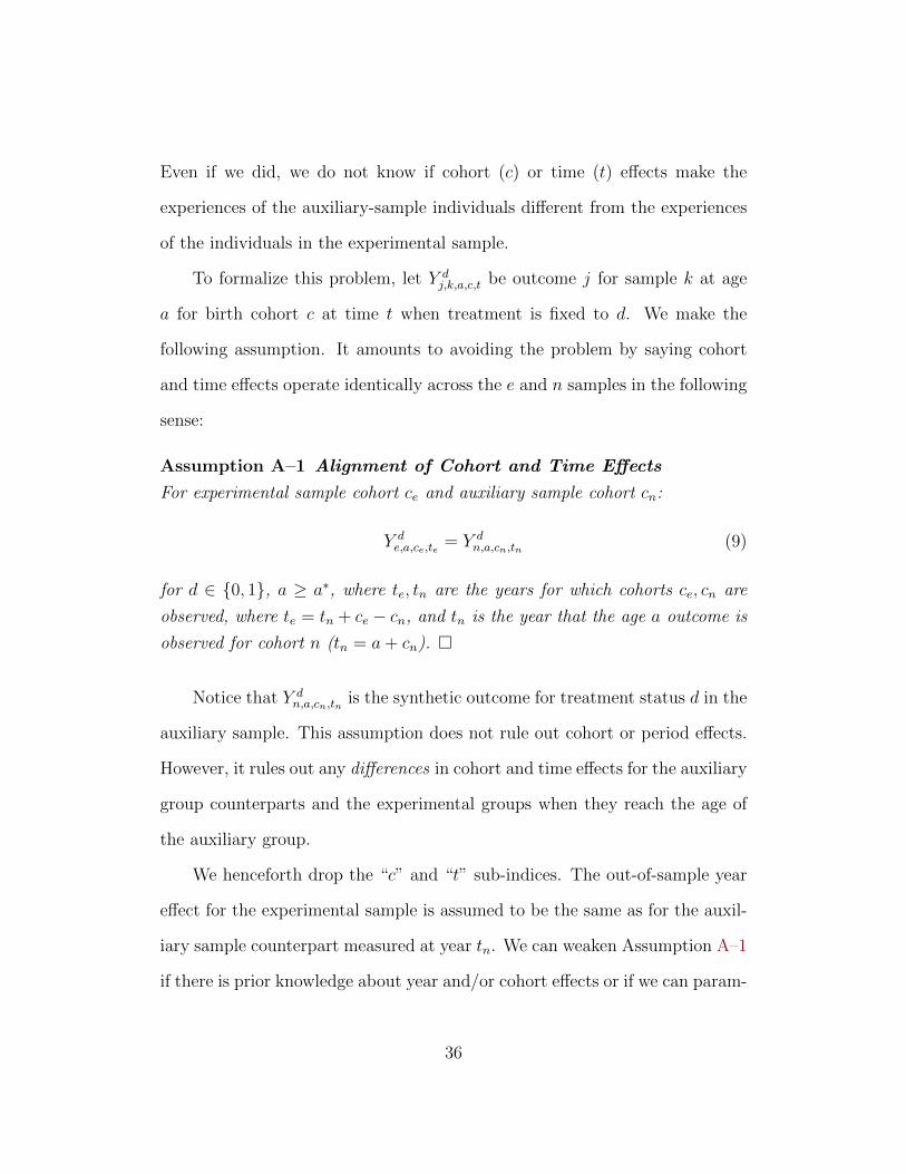
Even if we did, we do not know if cohort (c) or time (t) effects make the
experiences of the auxiliary-sample individuals different from the experiences
of the individuals in the experimental sample.
To formalize this problem, let Y dj,k,a,c,t be outcome j for sample k at age
a for birth cohort c at time t when treatment is fixed to d. We make the
following assumption. It amounts to avoiding the problem by saying cohort
and time effects operate identically across the e and n samples in the following
sense:
Assumption A–1 Alignment of Cohort and Time Effects
For experimental sample cohort ce and auxiliary sample cohort cn:
Y de,a,ce,te = Y d
n,a,cn,tn (9)
for d ∈ {0, 1}, a ≥ a∗, where te, tn are the years for which cohorts ce, cn are
observed, where te = tn + ce − cn, and tn is the year that the age a outcome is
observed for cohort n (tn = a+ cn). �
Notice that Y dn,a,cn,tn is the synthetic outcome for treatment status d in the
auxiliary sample. This assumption does not rule out cohort or period effects.
However, it rules out any differences in cohort and time effects for the auxiliary
group counterparts and the experimental groups when they reach the age of
the auxiliary group.
We henceforth drop the “c” and “t” sub-indices. The out-of-sample year
effect for the experimental sample is assumed to be the same as for the auxil-
iary sample counterpart measured at year tn. We can weaken Assumption A–1
if there is prior knowledge about year and/or cohort effects or if we can param-
36

eterize estimable functions of c and t.58 In the sensitivity analyses reported
below, we examine plausible alternative assumptions about cohort and time
effects.
5.2.2 Support Conditions
We require that the support of the auxiliary sample contains the support of
the experimental sample. This assumption allows us to find counterpart values
of Xdk,a, B, and Yk,a in the control and experimental samples.
Assumption A–2 Support Conditions
For a ∈ {1, . . . , A}, the support of(Y d
e,a,Xde,a,Be
)in the experimental sample
is contained in the support of(Y d
n,a,Xdn,a,Bn
)in the auxiliary sample:
supp(Ye,a,Xde,a,Be) ⊆ supp(Yn,a,X
dn,a,Bn), d ∈ {0, 1}. � (10)
This assumption is straightforward to test for ages a ≤ a∗. It is satisfied in
our samples. See Appendix C.3.5.
5.2.3 Conditions for Valid Out-of-Sample Predictions
A strong sufficient condition for identifying the distribution of life-cycle profiles
of individuals in the experimental sample using individuals in the auxiliary
samples is Condition C–1:
Condition C–1 Equality of Distributions Across the Experimental
and Auxiliary Samples
FY de ,Xd
e |Be=b (·, ·) = FY dn ,Xd
n|Bn=b (·, ·) , d ∈ {0, 1} (11)
58See Heckman and Robb (1985). For health, cohort effects could be very substantial (e.g.medical costs growth) and we account for this as explained in Section 5.4 and Appendix F.
37

for Y de ,X
de |Be = b and Y d
n ,Xdn|Bn = b contained in the support of the exper-
imental sample supp(Y d
e ,Xde ,Be
).
Since we are only interested in means for cost-benefit analysis, we can get
by with the following requirement for conditional means, which has testable
implications, as we show below:
Condition C–2 Equality in Conditional Expectations Across the Ex-
perimental and Auxiliary Samples
E[Y d
e |Xde = x,Be = b
]= E
[Y d
n |Xdn = x,Bn = b
], d ∈ {0, 1} (12)
for d ∈ {0, 1} over supp(Y d
e,a,Xde,a,Be
).
Since we are primarily interested in treatment effects, we can get by with
an even weaker condition:
Condition C–3 Equality in Mean Treatment Effects Across the Ex-
perimental and Auxiliary Samples
E[Y 1
e − Y 0e |Be = b
]= E
[Y 1
n − Y 0n |Bn = b
](13)
over supp(Y d
e,a,Be
).
We could simply invoke Condition C–2 or C–3 and be done. Our approach
is to examine and test (when possible) assumptions that justify them, and
Condition C–2 is useful for doing so.
5.2.4 Exogeneity
Conditions C–1 to C–3 do not require that we take a position on the exogeneity
of Xdk , k ∈ {e, n}. However, exogeneity facilitates the use of economic theory
38

to generate and interpret treatment effects, to test the validity of our synthetic
control groups, and to find auxiliary sample counterparts to treatments and
controls.59 For these purposes, we assume:
Assumption A–3 Exogeneity
For all a, a′′ ∈ {1, . . . , A} and for d, d′ ∈ {0, 1},
εdk,j,a ⊥⊥Xd′
k,a′′|Bk = b (14)
for all b in the support of Bk, k ∈ {e, n}, for all outcomes j ∈ Ja, where
“M ⊥⊥N |Q” denotes independence of M and N given Q. �
We test and do not reject this Assumption for a variety of outcomes in Ap-
pendix C.3.6. In Appendix C.6, we analyze standard panel data models for
the outcome equations as well as instrumental variable approaches to account
for lagged dependent variables and serial correlation, but our estimates are
robust even when we allow for different failures of Assumption A–3.
5.2.5 Structural Invariance
We assume that the variables Xdk,a fully summarize treatment in the sense that
any effect that treatment has on outcomes operates through the inputs Xdk,a
and not through shifts in the production function relating inputs to outputs
(see Heckman et al., 2013). Assumption A–4 formalizes this statement.
Assumption A–4 Structural Invariance
59It also facilitates matching, one of the methods used in this paper. See Heckman andNavarro (2004).
39

For all x, b ∈ supp(Xde,a,Be), k ∈ {e, n}
φ0k,j,a (x, b) = φ1
k,j,a(x, b) (15)
=: φj,a(x, b),
φdk,j,a(x) is the function generating the causal effect of setting Xd
k,a = x holding
εdk,j,a fixed for a ∈ {1, . . . , A} for any outcome j ∈ Ja. �
This assumption has two distinct messages: (i) the structural functions
evaluated at the same arguments have identical values for treatment and con-
trol groups in the experimental sample. It also says (ii) that the structural
relationships are identical in the experimental and auxiliary samples. As pre-
viously noted, exogeneity is not needed to justify any of the Conditions C–
1 through C–3. But in the absence of exogeneity, the relationship between
the Xdk,a and the errors εdk,a likely differs across experimental (e) and non-
experimental (n) samples because randomization imparts a source of exoge-
nous variation to the Xde,a not present in non-experimental samples. Assump-
tion A–4 combined with Assumption A–3, Equation (8), and the assumption
of a zero mean for the errors (E(εdk,j,a) = 0) for all a ∈ {1, . . . , A}, d ∈ {0, 1}
and k ∈ {e, n} enable us to write:
E[Y dk,j,a|Xd
k,a = x,Bk = b, D = d]
= E[Yk,j,a|Xd
k,a = x,Bk = b], (16)
for a ∈ {1, . . . , A}, k ∈ {e, n}, and d ∈ {0, 1}.
40

5.2.6 Testable Implications
Equation (16) relates outcomes for Y dk,j,a to treatment effects for Xd
k,a, together
with the background variables Bk. It is possible to test A–4 within the ex-
perimental sample (a ≤ a∗). The test consists of asking if Xde,a,B predict
the within-experimental sample treatment effects for Ye,j,a. Under the null
hypothesis that A–4 is correct, a separate indicator variable for treatment sta-
tus (d) is irrelevant when computing E[Ye,j,a|Xd
k,a = x,Bk = b, D = d]. In
Appendix C.3.7, we test and do not reject the null hypotheses.60
Exogeneity and invariance enable us to test additional assumptions. By
Equation (16), we can write:
E[Ye,j,a|Xd
e,a = x,Be = b]
= E[Yn,j,a|Xd
n,a = x,Bn = b]
(17)
for d ∈ {0, 1} a ∈ {1, . . . , A}.
Relationship (17) is testable for a ≤ a∗, when Yk,j,a is observed in both
the experimental and auxiliary samples. We do not reject the null hypotheses
of no differences in the conditional mean functions in the experimental and
auxiliary samples conditioning on Xdk,a and Bk, k ∈ {e, n}.61
5.2.7 Summarizing the Implications of Exogeneity and Structural
Invariance
Collecting results, we obtain the following theorem:
60This holds both when pooling males and females and when testing separately by gender(see Appendix C.3.7).
61This holds when pooling males and females and when testing by gender (see Ap-pendix C.3.7).
41

Theorem 1 Valid Out-of-Sample Predictions
Under Assumptions A–1-A–4, Conditions C–2 through C–3 hold for any value
of(Xd
k,a,Bk
).
This is an immediate consequence of the cited assumptions. �
5.2.8 Testing for Endogeneity
In Appendix C.3.6, we report tests for endogeneity in the experimental and
auxiliary samples used in this paper. We follow Heckman et al. (2013) and
assume that the εdk,j,a obey a factor structure, k ∈ {e, n}. We develop that
framework and provide evidence supporting exogeneity in both samples for
the predictor variables used in our empirical analyses.
5.2.9 Using Matching to Construct Virtual Treatment and Com-
parison Groups
Under exogeneity assumption A–3 and invariance condition A–4 we can use
matching to construct counterparts to treatment and control groups in the
auxiliary sample.62 Doing so compresses the two stages of constructing a com-
parison group and creating predictions into one stage. Matching in this fash-
ion creates direct auxiliary counterparts for each member of the experimental
samples. It is an intuitively appealing estimator.
We discuss this approach in Appendix C.3.3. Matching is a non-parametric
estimator of the conditional mean functions. There is close agreement between
non-parametric estimates based on matching and more parametric model-
based approaches like the one we use throughout the main text (see Ap-
62Heckman et al. (1998) use this procedure.
42

pendix C.3.4.1).
5.2.10 Summarizing Our Approach and What We Do in This Paper
Using the data sources listed in Table 5, we execute our analysis in two stages.
In Stage I, we construct comparison samples using background variables (Bn).
In Stage II, we use the samples so constructed to create post-a∗ prediction
models based on B and Xde . We repeat that the structural invariance and
exogeneity assumptions discussed in this section are sufficient conditions for
justifying Conditions C–2 and C–3. We can clearly weaken these assumptions.
For example, creating mean difference counterfactuals only requires exogeneity
and structural invariance in mean differences, and not in individual level equa-
tions. However, the conditions stated for level equations by treatment status
have the advantage of being testable on certain subsamples of the data. They
also justify matching to make valid predictions. Appendix C.6 reports esti-
mates from a variety of alternative approaches accounting for serial correlation
in the errors and from non-parametric matching.
5.3 Predicting Parental Labor Income
ABC/CARE offers childcare to the parents of treated children for more than
nine hours a day for five years, 50 weeks a year. Only 27% of mothers of chil-
dren reported living with a partner at baseline and this status barely changed
during the course of the experiment (see Appendix A). The childcare compo-
nent generates the treatment effects in maternal labor force participation and
parental labor income reported in Tables 3 and 4 and Appendix G.
43

We observe parental labor income at eight different times for the exper-
imental subjects up through age 21.63,64 As Tables 3 and 4 show, treatment
effects on parental labor income are sustained through the child’s age 21. This
presumably arises from wage growth due to parental attainment of further
education and/or more work experience. An ideal approach would be to esti-
mate the profile over the full life cycle of mothers. We propose two different
approaches for doing this in Appendix C.3.8: (i) an approach based on param-
eterizing parental labor income using standard Mincer equations; and (ii) an
approach based on the analysis of Section 5.2. In Section 6, we present esti-
mates using the labor income through age 21 and using these two alternatives
for projecting future labor income after age 21. The benefits of the program
increase when considering the full life cycles of mothers using either approach.
Any childcare inducements of the program likely benefit parents who, at
baseline, did not have any other children. If they did, then they might have had
to take care of other children anyway, weakening the childcare-driven effect,
especially if there are younger siblings present. In Appendix C.3.8, we show
that the treatment effect for discounted parental labor income is much higher
when there are no siblings of the participant children at baseline. The effect
also weakens when comparing children who have siblings younger than 5 years
old to children who have siblings 5 years old or younger.65
63The ages at which parental labor income is observed are 0, 1.5, 3.5, 4.5, 8, 12, 15, and21. At age 21 the mothers in ABC/CARE were, on average, 41 years old.
64We linearly interpolate parental labor income for ages for which we do not have obser-vations between 0 and 21.
65These patterns persist when splitting the ABC/CARE sample by gender, but the esti-mates are not precise because the samples become too small. See Appendix C.3.8.
44

5.4 Health
We predict and monetize health outcomes based on a version of Equation (7)
including a full vector of lagged dependent variables for different indicators
of health status. This requires adapting the models of Section 5.2. Three
additional issues arise: (i) health outcomes such as diabetes or heart disease
are absorbing states; (ii) health outcomes are highly interdependent within
and across time periods; and (iii) there is no obvious terminal time period for
benefits and costs except death, which is endogenous.66
Our auxiliary model for health is an adaptation of the Future America
Model (FAM). This model predicts health outcomes from the subjects’ mid-
30s up to their projected age of death (Goldman et al., 2015).67 Appendix F
discusses the FAM methodology in detail.
In Appendix F, we present tests of its assumptions and its predictive
performance for population aggregate health and healthy behavior outcomes.
FAM passes a variety of specification tests and accurately predicts health out-
comes and healthy behaviors. We initialize the health prediction model using
the same variables that we use to predict labor and transfer income, along
with the initial health conditions as listed in Table 6.
Our methodology has five steps: (i) estimate age-by-age health state
transition probabilities using the Panel Study of Income Dynamics (PSID);
(ii) match these transition probabilities to the ABC/CARE subjects based
on observed characteristics; (iii) estimate quality-adjusted life year (QALY)
66For example, for income we extrapolate up to the retirement age of 67. However, forhealth, we need to predict an age of death for each individual.
67The simulation starts at the age in which we observe the subject’s age-30 follow-up.
45

models using the Medical Expenditure Panel Survey (MEPS) and the PSID;
(iv) estimate medical cost models using the MEPS and the Medicare Current
Beneficiary Survey (MCBS), allowing estimates to differ by health state and
observed characteristics; and (v) predict the medical expenditures and QALYs
that correspond to the simulated individual health trajectories.68
Our microsimulation model starts with health predictions for age 30, along
with the information on observed characteristics available at this age. Restrict-
ing it to the individuals for whom we have information from the mid-30s health
survey allows us to account for components that are important for predicting
health outcomes. The models predict the probability of being in any of the
states in the horizontal axis of Table 6 at age a+1 based on the state at age a,
which is described by the vertical axis of the table.69 Absorbing states are an
exception. For example, heart disease at age a does not enter in the estimation
of transitions for heart disease at age a + 1 because it is an absorbing state:
once a person has heart disease, she carries it through the rest of her life.
At each age, once we obtain the transition probability for each health out-
come, we make a Monte-Carlo draw for each subject. Thus, each simulation
depends on each individual’s health history and on their particular charac-
teristics. For every simulated trajectory of health outcomes, we predict the
lifetime medical expenditure using the models estimated from the MEPS and
the MCBS. We then obtain an estimate of the expected lifetime medical ex-
68As an intermediate step between (i) and (ii), we impute some of the variables used toinitialize the FAM models (see Appendix F).
69In practice, the predictions are based on two-year lags, due to data limitations in theauxiliary sources we use to simulate the FAM. For example, if the individual is 30 (31) yearsold in the age-30 interview, we simulate the trajectory of her health status at ages 30 (31),32 (33), 34 (35), and so on until her projected death.
46

Tab
le6:
Hea
lth
Sta
teT
ransi
tion
s,A
gea
asP
redic
tor
ofA
gea
+1
Agea
Agea
+1
Heart
Hyp
er-
Str
oke
Lung
Dia
bete
sC
ancer
Dis
abilit
yM
ort
ality
Sm
okin
gO
besi
tyH
ealt
hD
ISS
SSI
Dis
ease
tensi
on
Dis
ease
Insu
rance
Cla
imC
laim
Cla
imH
eart
Dis
ease
××
××
××
××
Hyp
ert
ensi
on
××
××
××
××
Str
oke
××
××
××
Lung
Dis
ease
××
××
××
×D
iab
ete
s×
××
××
××
××
×C
ancer
××
××
××
×D
isabilit
y×
××
××
×
Sm
okin
g×
××
××
××
××
××
××
BM
I×
××
××
××
××
Physi
cal
Acti
v.
××
××
××
××
Bin
ge
Dri
nkin
g×
×
DI
Cla
im×
××
×SS
Cla
im×
×SSI
Cla
im×
Not
e:T
his
tab
leil
lust
rate
sh
owh
ealt
hou
tcom
esat
age
ap
red
ict
hea
lth
ou
tcom
esat
agea
+1.
Th
ecr
oss
esin
dic
ate
ifw
eu
seth
eag
ea
outc
ome
top
red
ict
the
agea
+1
outc
ome.
DI
Cla
im:
pay
roll
-tax
fun
ded
,fe
der
al
insu
ran
cep
rogra
mfo
rin
div
idu
als
wh
ow
ork
lon
gen
ough
pay
ing
Soci
alS
ecu
rity
taxes
;S
SC
laim
:old
-age
surv
ivors
an
dd
isab
ilit
yin
sura
nce
pro
gra
mco
llec
ted
thro
ugh
pay
roll
taxes
by
the
Inte
rnal
Rev
enu
eS
ervic
e;S
SI
Cla
im:
claim
sof
stip
end
sfo
rlo
w-i
nco
me
peo
ple
wh
oare
old
erth
an
65
yea
rsold
,b
lind
,or
dis
able
d.
47

penditure by taking the mean of each individual’s simulated lifetime medical
expenditure.
The models estimated using MCBS represent medical costs in the years
2007-2010. The MEPS estimation captures costs during 2008-2010. To ac-
count for real medical cost growth after 2010, we adjust each model’s predic-
tion using the method described in Appendix F.
Figure 6: Quality Adjusted Life Years: Predictions and Comparison to PSID
5
5.1
5.2
5.3
5.4
QA
LY
s (
10
0,0
00
s 2
01
4 U
SD
)
Males Females
PSID, Disadvantaged Control (Predicted) Treatment (Predicted)
+/− s.e.
Note: This figure displays the life-cycle net-present value of predicted quality-adjusted lifeyears (QALYs) for ABC/CARE males and females, respectively, by treatment status. Thepredictions are based on combining data from the Panel Study of Income Dynamics (PSID),the Health Retirement Study, and the Medical Expenditure Panel Survey (MEPS). For eachgender, we display a comparison to disadvantaged males and females in the Panel Studyof Income Dynamics (PSID), where disadvantaged is defined as being Black and having 12years of education or less. QALYs are the quality-adjusted life years gain due to betterhealth conditions. Standard errors are based on the empirical bootstrap distribution.
The same procedure is applied to calculate quality-adjusted life years
(QALYs).70 We compute a QALY model based on a widely-used health-related
70A quality-adjusted life year (QALY) reweights a year of life according to its qualitygiven the burden of disease. Suppose we assign a value of $150, 000 (2014 USD) to each
48

Quality-of-Life (HRQoL) measure (EQ-5D), available in MEPS.71 We then es-
timate this model using the PSID.
We estimate three models of medical spending: (i) Medicare spending
(annual medical spending paid by parts A, B, and D of Medicare); (ii) out-of-
pocket spending (medical spending paid directly by the individual); and (iii) all
public spending other than Medicare. Each medical spending model includes
the variables we use to predict labor and transfer income, together with current
health, risk factors, and functional status as explanatory variables.
We also calculate medical expenditure before age 30. The ABC/CARE
interviews at ages 12, 15, 21 and 30 have information related to hospitaliza-
tions at different ages and number of births before age 30. We combine this
information along with individual and family demographic variables to use
MEPS to predict medical spending for each age.
QALYs are crucial for our benefit-cost analysis because they monetize the
health of an individual at each age. Figure 6 shows our estimation of QALYs
together with a PSID comparison, in an exercise analogous to that used to
produce Figure 4.72 Although there is not a clear age-by-age treatment effect
year of life. A QALY of $150, 000 denotes a year of life in the absence of disease (perfecthealth). The value of QALY for an individual in a given year is smaller than $150, 000when there is positive burden of disease, as worse health conditions imply lower QALYs.When an individual dies, her QALY equals zero. There are extreme combinations of diseaseand disability that may generate negative QALYs, although this is unusual. Because wequantify labor income in addition to other components, this value corresponds solely tomonetizing the value of life net of what individuals produce in terms of economic output.The benefit-cost ratio and internal rate of return remain significant after removing thiscomponent entirely (see Table 9).
71For a definition and explanation of this instrument, see Dolan (1997); Shaw et al.(2005).
72In our baseline estimation, we assume that each year of life is worth $150, 000 (2014USD). Our estimates are robust to substantial variation in this assumption, as we show inAppendix I.
49

on QALYs, there is a statistically and substantively significant difference in
the accumulated present value of the QALYs between the treatment and the
control groups. The QALYs for individuals in the control group match the
QALYs of disadvantaged individuals in the PSID.73
5.5 Crime
To estimate the life-cycle benefits and costs of ABC/CARE related to crimi-
nal activity, we use rich data on crime outcomes obtained from public police
records.74 See Appendix E for a more complete discussion. We consider the
following types of crime: arson, assault, burglary, fraud, larceny, miscella-
neous (which includes traffic and non-violent drug crimes which can lead to
incarceration), murder, vehicle theft, rape, robbery, and vandalism. We use
administrative data that document: (i) youth arrests, gathered at the age-21
follow-up; (ii) adult arrests, gathered at the mid-30’s follow-up; and (iii) sen-
tences, gathered at the mid-30’s follow-up. We also use self-reported data on
adult crimes, gathered in the age-21 and age-30 subject interviews. Because
none of these sources capture all criminal activity, it is necessary to combine
them to more completely approximate the crimes the subjects committed. We
also use several auxiliary datasets to complete the life-cycle profile of criminal
activity and compute the costs of the committed crimes.
73In Appendix F we further discuss and justify the parameterizations required to obtainestimates of QALYs. Tysinger et al. (2015) examine the sensitivity to these parameteriza-tions and discuss alternative micro-simulations monetizing health condition.
74Two previous studies consider the impacts of ABC on crime: Clarke and Campbell(1998) use administrative crime records up to age 21, and find no statistically significantdifferences between the treatment and the control groups. Barnett and Masse (2002, 2007)account for self-reported crime at age 21. They find weak effects, but they lack access tolonger term, administrative data.
50

We follow four steps to estimate the costs of crime.
1. Count arrests and sentences. We start by counting the total number of
sentences for each individual and type of crime (arson, assault, etc.) up
to the mid 30’s, matching crimes across data sources, to construct the
total number of arrests for each individual and type of crime up to the
mid 30’s.75 For individuals missing arrest data,76 we impute the number
of arrests by multiplying the number of sentences for each type of crime
by a national arrest-sentence ratio for the respective crime.77
2. Construct predictions. Based on the sentences observed before age mid
30’s, we predict the sentences that the ABC/CARE subjects will have
after age mid 30’s. Data from the North Carolina Department of Pub-
lic Safety (NCDPS), which provide lifetime sentences of individuals in
North Carolina, are used to estimate sentences incurred after age mid
30’s from sentences incurred before age mid 30’s. Applying these models
to the ABC/CARE data, we predict the number of future sentences for
each subject up to age 50.78 We then add these estimates to the orig-
inal number of sentences, getting an estimate of the lifetime sentences.
75In practice, we count all offenses (an arrest might include multiple offenses). This givesthe correct number of victims for our estimations. The youth data have coarser categoriesthan the rest of the data: violent, property, drug, and other. To match these data with theadult data, we assume that all property crimes were larcenies and that all violent crimesare assaults. In the ABC/CARE sample, assault is the most common type of violent crime,and larceny/theft is the most common property crime.
76About 10% of the ABC/CARE sample has missing arrest data. We fail to reject thenull hypothesis of no differences in observed characteristics between the treatment- andcontrol-group participants for whom we observe arrests data (see Appendix A.6).
77This arrest-sentence ratio is constructed using the National Crime Victimization Survey(NJRP) and the Uniform Crime Reporting Statistics (UCRS).
78We assume that individuals with no criminal records before age mid 30’s commit nocrimes after age mid 30’s.
51

Adding these estimates increases the total count of crimes by 30%–50%.
3. Estimate number of victims from the crimes. We only observe crimes
that resulted in consequences in the justice system: crimes that resulted
in arrests and/or sentences. To include unobserved crimes, we use vic-
timization inflation (VI).79 We start by constructing a VI ratio, which
is the national ratio of victims and arrests for each type of crime.80
Then, we estimate the number of victims from the crimes committed by
ABC/CARE subjects as their total arrests multiplied by the VI ratio.81
4. Find total costs of crimes. We use the estimates of the cost of crimes
for victims from McCollister et al. (2010) to impute the total victimiza-
tion costs. For crimes resulting in arrests and/or sentences, we consider
justice system costs as well, such as police costs.82 Finally, we construct
the total costs of incarceration for each subject using the total prison
time and the cost of a day in prison.83
79Previous papers using this method include Belfield et al. (2006) and Heckman et al.(2010b).
80We assume that each crime with victims is counted separately in the national reportson arrests, even for arrests that might have been motivated by more than one crime. Thisvictim-arrest ratio is constructed using the NJRP and the National Crime VictimizationSurvey (NCVS).
81Additionally, we can calculate an analogous estimate of the number of crime victimsusing sentences, based on the VI ratio and the national arrests-to-sentences ratio. Theseestimates are very similar, as shown in Appendix E. To improve precision, the estimates inthe rest of our paper are based on the average of the two calculations.
82To be able to assign costs to each type of crime, we assume that the cost of the justicesystem depends on the number of offenses of each type, rather than on the number ofarrests. While this could very slightly overestimate justice system costs, the costs onlyrepresent about 5% of the total crime costs.
83Appendix I examines the sensitivity of our crime costs quantification to different as-sumptions. Section 6 and Appendix I we examine the sensitivity of our overall assessmentof ABC/CARE results to the quantification of crime that we explain in this section.
52

5.6 Education
Follow-up data on educational attainment were collected through age 30. In
Appendix D, we show that using auxiliary data sources, education up to this
age is an accurate predictor of lifetime educational attainment. Therefore, we
do not predict educational attainment beyond age 30. To monetize the costs
of education, we consider the public costs of K-12 education and the public
and private costs of post-secondary education, including vocational programs
and community college. Other costs of education include grade retention and
special education. Previous analyses of ABC pay special attention to special
education, arguing that savings due to a reduction in this category are substan-
tial (Barnett and Masse, 2002, 2007).84 This category is much less important
in our calculation.85
6 Benefit/Cost Analysis
This section reports benefit/cost and rate of return analyses underlying Fig-
ure 1. Appendix I displays an extensive sensitivity analysis of each of the
components we consider. It includes scenarios in which all of our assump-
tions hold and scenarios in which they are violated, providing bounds for our
estimates.
84Their analyses do not include CARE.85Pooling males and females the net gain due to a reduction in special education is
$9, 724.4 (2014 USD) (s.e. $8, 608.1). For males the gain is $14, 694.9 (2014 USD) (s.e.$11, 065.4) and for females it is $4, 077.5 (2014 USD) (s.e. $14, 892.0). This quantity isdiscounted to the child’s birth.
53

6.1 Program Costs
The yearly cost of the program was $18,514 per participant in 2014 USD. We
improve on previous cost estimates using primary-source documents.86
6.2 Benefit/Cost Estimates
Table 7 presents our baseline estimates of benefit/cost ratios, Table 8 presents
the analogous internal rates of return. Pooling males and females, the results
indicate that the program is socially efficient: the internal rate of return and
the benefit/cost ratio are 13.7% and 7.3. The program generates a benefit
of 7.3 dollars for every dollar spent on it. These estimates are statistically
significant, even after accounting for sampling variation, serial correlation,
and prediction error in the experimental and auxiliary samples and the tax
costs of financing the program.87 These benefits arise despite the fact that
ABC/CARE was much more expensive than other early childhood education
programs—the treatment involved more services over a longer time period
(Elango et al., 2016).
86Our calculations are based on progress reports written by the principal investigators andrelated documentation recovered in the archives of the research center where the programwas implemented. We display these sources in Appendix B. The main component is staffcosts. Other costs arise from nutrition and services that the subjects receive when theywere sick, diapers during the first 15 months of their lives, and transportation to the center.The control-group children also receive diapers during approximately 15 months, and iron-fortified formula. The costs are based on sources describing ABC treatment for 52 children.We use the same costs estimates for CARE, for which there is less information available.The costs exclude any expenses related to research or policy analysis. A separate calculationby the implementers of the program indicates almost an identical amount (see Appendix B).
87We obtain the reported standard errors by bootstrapping all steps of our empiricalprocedure, including variable selection, imputation, model selection steps, and predictionerror (see Appendix C.8).
54

We accompany these estimates with a set of sensitivity checks of statisti-
cal and economic interest. Our estimates are not driven by our methods for
accounting for attrition and item non-response or by the conditioning variables
we use when computing the net-present values. Although the internal rate of
return remains relatively high when using participant outcome measures up to
ages 21 or 30, the benefit/cost ratios indicate that accounting for benefits that
go beyond age 30 is important. The return to each dollar is at most 3/1 when
considering benefits up to age 30 only (prediction span columns). Accounting
for the treatment substitutes available to controls also matters. Males benefit
the most from ABC/CARE relative to attending alternative childcare centers,
while females benefit the most from ABC/CARE relative to staying at home.
We explore this difference below.
Our baseline estimates account for the deadweight loss caused by the
government using distortionary taxes to fund programs, plus the direct costs
associated with collecting taxes.88 Our baseline estimate assumes that the
marginal tax rate is 50%.89 Our estimates are robust to dropping it to 0%
or doubling it to 100% (deadweight loss columns). Our baseline estimate of
benefit/cost ratios is based on a discount rate of 3%. Not discounting roughly
doubles our benefit/cost ratios, while they remain statistically significant using
88When the transaction between the government and an individual is a direct transfer,we consider 0.5 as a cost per each transacted dollar as we do not weight the final recipientof the transaction (e.g., transfer income). When the transaction is indirect, we classify itas government spending as a whole and consider its cost as 1.5 per each dollar spent (e.g.,public education).
89Feldstein (1999) reports that the deadweight loss caused by increasing existing tax rates(marginal deadweight loss) may exceed two dollars per each dollar of revenue generated.We use a more conservative value (0.5 dollars per each dollar of revenue generated). InTables 7, 8, and 9 and in Appendix I, we explore the robustness of this decision and findlittle sensitivity.
55

Tab
le7:
Sen
siti
vit
yA
nal
ysi
sfo
rB
enefi
t/C
ost
Rat
ios
Poole
dM
ale
sF
em
ale
s
Base
lin
e7.3
3(s
.e.
1.8
4)
10.1
9(s
.e.
2.9
3)
2.6
1s.
e.0.7
3)
Baseline:
IPW
andControls,Life-spanupto
predicteddeath,Treatm
entvs.NextBest,
50%
Marginaltax50%
(deadweigh
tloss),
Discountrate
3%,Parental
income0to
21(child’s
age),
LaborIn
comepredictedfrom
21to
65,Allcrim
es(fullcosts),Valueoflife
150,000.
Sp
ecifi
cati
on
NoIP
WandNoControls
NoIP
WandNoControls
NoIP
WandNoControls
7.3
17.9
99.8
08.8
32.5
72.8
2(1
.81)
(2.1
8)
(2.6
9)
(2.7
2)
(0.7
2)
(0.6
8)
Pred
icti
on
toAge
21
toAge
30
toAge
21
toAge
30
toAge
21
toAge
30
Sp
an
1.5
23.1
92.2
33.8
41.4
61.8
1(0
.36)
(1.0
4)
(0.6
1)
(1.6
0)
(0.3
6)
(0.5
0)
Cou
nte
r-
vs.StayatHome
vs.Alt.Presch.
vs.StayatHome
vs.Alt.Presch.
vs.StayatHome
vs.Alt.Presch.
factu
als
5.4
49.6
33.3
011.4
65.7
92.2
8(1
.86)
(3.1
0)
(2.9
5)
(3.1
6)
(1.3
7)
(0.7
6)
Dead
weig
ht-
0%
100%
0%
100%
0%
100%
loss
11.0
15.5
015.3
87.5
93.8
32.0
1(2
.79)
(1.3
7)
(4.3
5)
(2.2
3)
(1.0
4)
(0.5
9)
Dis
cou
nt
0%
7%
0%
7%
0%
7%
Rate
17.4
02.9
125.4
53.7
85.0
61.4
9(5
.90)
(0.5
9)
(10.4
2)
(0.7
9)
(2.8
2)
(0.3
2)
Parenta
lMincerLife-cy
cle
Life-cy
clePrediction
MincerLife-cy
cle
Life-cy
clePrediction
MincerLife-cy
cle
Life-cy
clePrediction
Incom
e7.6
37.7
310.4
610.6
32.9
83.1
2(1
.84)
(1.9
2)
(2.9
4)
(2.9
5)
(0.7
6)
(0.8
5)
Lab
or
.5%
AnnualDecay
.5%
AnnualGrowth
.5%
AnnualDecay
.5%
AnnualGrowth
.5%
AnnualDecay
.5%
AnnualGrowth
Incom
e7.0
17.6
69.5
810.7
92.5
12.7
1(1
.80)
(1.9
0)
(2.6
6)
(3.2
4)
(0.7
0)
(0.7
5)
Crim
eDropMajorCrimes
HalveCosts
DropMajorCrimes
HalveCosts
DropMajorCrimes
HalveCosts
4.2
45.1
87.4
17.1
22.6
12.4
7(1
.10)
(1.2
2)
(3.4
3)
(2.4
1)
(0.6
7)
(0.6
6)
Healt
hDropAll
DoubleValueofLife
DropAll
DoubleValueofLife
DropAll
DoubleValueofLife
(QA
LY
s)6.4
88.1
99.1
411.2
32.2
03.0
3(1
.79)
(2.1
3)
(2.7
3)
(3.4
0)
(0.6
9)
(1.0
4)
Note
:T
his
tab
led
isp
lays
sen
siti
vit
yan
aly
ses
of
ou
rb
ase
lin
eb
enefi
t/co
stra
tio
calc
ula
tion
toth
ep
ertu
rbati
on
sin
dex
edin
the
diff
eren
tro
ws.
Th
ech
ara
cter
isti
csof
thebaseline
calc
ula
tion
are
inth
eta
ble
hea
der
.IP
W:
ad
just
sfo
ratt
riti
on
an
dit
emn
on
-res
pon
se(s
eeA
pp
end
ixC
.2fo
rd
etails)
.C
ontr
ol
vari
ab
les:
Ap
gar
score
sat
ages
1an
d5
an
da
hig
h-r
isk
ind
ex(s
eeA
pp
end
ixG
for
det
ails
on
how
we
choose
thes
eco
ntr
ols
).W
hen
pre
dic
tin
gu
pto
ages
21
an
d30,
we
con
sid
erall
ben
efits
an
dco
sts
up
toth
ese
ages
,re
spec
tivel
y.C
ou
nte
rfact
uals
:w
eco
nsi
der
trea
tmen
tvs.
nex
tb
est
(base
lin
e),
trea
tmen
tvs.
stay
at
hom
e,an
dtr
eatm
ent
vs.
alt
ern
ati
ve
pre
schools
(see
Sec
tion
2fo
ra
dis
cuss
ion
).D
ead
wei
ght
loss
isth
elo
ssim
pli
edby
any
pu
blic
exp
end
itu
re(0
%is
no
loss
an
d100%
ison
ed
ollar
loss
per
each
dollar
spen
t).
Dis
cou
nt
rate
:ra
teto
dis
cou
nt
ben
efits
toch
ild
’sage
0(i
nall
calc
ula
tion
s).
Pare
nta
lla
bor
inco
me:
see
Ap
pen
dix
C.3
.8fo
rd
etails
on
the
two
alt
ern
ati
ve
pre
dic
tion
s(M
ince
ran
dL
ife-
cycl
e).
Lab
or
Inco
me:
0.5
an
nu
al
gro
wth
(dec
ay)
isan
an
nu
al
wage
gro
wth
(dec
ay)
du
eto
coh
ort
effec
ts.
Cri
me:
ma
jor
crim
esare
rap
ean
dm
urd
er;
half
cost
sta
kes
half
of
vic
tim
izati
on
an
dju
dic
iary
cost
s.H
ealt
h(Q
ALY
s):
dro
pall
sets
the
valu
eof
life
equ
al
toze
ro.
Sta
nd
ard
erro
rsob
tain
edfr
om
the
emp
iric
al
boots
trap
dis
trib
uti
on
are
inp
are
nth
eses
.B
old
edp-v
alu
esare
sign
ifica
nt
at
10%
usi
ng
on
e-si
ded
test
s.F
or
det
ails
on
the
nu
llhyp
oth
esis
see
Tab
le9.
56
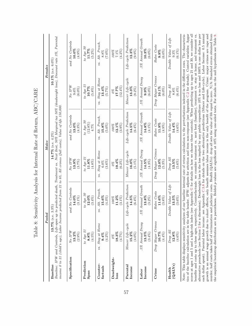
Tab
le8:
Sen
siti
vit
yA
nal
ysi
sfo
rIn
tern
alR
ate
ofR
eturn
,A
BC
/CA
RE
Poole
dM
ale
sF
em
ale
s
Base
lin
e13.7
%(s
.e.
3.3
%)
14.7
%(s
.e.
4.2
%)
10.1
%(s
.e.
6.0
%)
Baseline:
IPW
andControls,Life-spanupto
predicteddeath,Treatm
entvs.NextBest,
50%
Marginaltax50%
(deadweigh
tloss),
Discountrate
3%,Parental
income0to
21(child’s
age),
LaborIn
comepredictedfrom
21to
65,Allcrim
es(fullcosts),Valueoflife
150,000.
Sp
ecifi
cati
on
NoIP
WandNoControls
NoIP
WandNoControls
NoIP
WandNoControls
13.2
%14.0
%13.9
%13.0
%9.6
%10.0
%(2
.9%
)(3
.1%
)(3
.7%
)(4
.3%
)(6
.0%
)(4
.9%
)
Pred
icti
on
toAge
21
toAge
30
toAge
21
toAge
30
toAge
21
toAge
30
Sp
an
8.8
%12.0
%11.8
%(1
2.8
%)
10.7
%11.7
%(4
.5%
)(3
.4%
)(4
.8%
)4.7
%(5
.8%
)(5
.2%
)
Cou
nte
r-
vs.StayatHome
vs.Alt.Presch.
vs.StayatHome
vs.Alt.Presch.
vs.StayatHome
vs.Alt.Presch.
factu
als
9.4
%15.6
%6.0
%15.8
%13.4
%8.8
%(4
.2%
)(4
.3%
)(3
.6%
)(5
.0%
)(5
.7%
)(7
.0%
)
Dead
weig
ht-
0%
100%
0%
100%
0%
100%
loss
18.3
%11.2
%19.4
%12.1
%17.7
%7.1
%(4
.7%
)(3
.1%
)(6
.2%
)(3
.9%
)(1
2.4
%)
(4.2
%)
Parenta
lMincerLife-cy
cle
Life-cy
clePrediction
MincerLife-cy
cle
Life-cy
clePrediction
MincerLife-cy
cle
Life-cy
clePrediction
Incom
e15.2
%14.5
%16.0
%14.5
%13.3
%12.3
%(4
.0%
)(6
.4%
)(5
.1%
)(6
.4%
)(8
.2%
)(9
.9%
)
Lab
or
.5%
AnnualDecay
.5%
AnnualGrowth
.5%
AnnualDecay
.5%
AnnualGrowth
.5%
AnnualDecay
.5%
AnnualGrowth
Incom
e13.5
%13.8
%14.5
%14.8
%9.9
%10.3
%(3
.4%
)(3
.2%
)(4
.3%
)(4
.1%
)(6
.0%
)(6
.0%
)
Crim
eDropMajorCrimes
HalveCosts
DropMajorCrimes
HalveCosts
DropMajorCrimes
HalveCosts
10.7
%11.6
%12.0
%11.9
%10.1
%9.9
%(4
.4%
)(3
.8%
)(5
.3%
)(4
.9%
)(6
.0%
)(6
.0%
)
Healt
hDropAll
DoubleValueofLife
DropAll
DoubleValueofLife
DropAll
DoubleValueofLife
(QA
LY
s)12.8
%13.5
%13.5
%14.4
%8.8
%9.3
%(4
.6%
)(3
.6%
)(5
.6%
)(4
.6%
)(6
.4%
)(6
.1%
)
Note
:T
his
tab
led
isp
lays
sen
siti
vit
yan
aly
ses
of
ou
rb
ase
lin
ein
tern
al
rate
of
retu
rnca
lcu
lati
on
toth
ep
ertu
rbati
on
sin
dex
edin
the
diff
eren
tro
ws.
Th
ech
ara
cter
is-
tics
of
thebaseline
calc
ula
tion
are
inth
eta
ble
hea
der
.IP
W:
ad
just
sfo
ratt
riti
on
an
dit
emn
on
-res
pon
se(s
eeA
pp
end
ixC
.2fo
rd
etails)
.C
ontr
ol
vari
ab
les:
Ap
gar
score
sat
ages
1an
d5
an
da
hig
h-r
isk
ind
ex(s
eeA
pp
end
ixG
for
det
ails
on
how
we
choose
thes
eco
ntr
ols
).W
hen
pre
dic
tin
gu
pto
ages
21
an
d30,
we
con
sid
erall
ben
efits
an
dco
sts
up
toth
ese
ages
,re
spec
tivel
y.C
ou
nte
rfact
uals
:w
eco
nsi
der
trea
tmen
tvs.
nex
tb
est
(base
lin
e),
trea
tmen
tvs.
stay
at
hom
e,an
dtr
eatm
ent
vs.
alt
ern
ati
ve
pre
sch
ools
(see
Sec
tion
2fo
ra
dis
cuss
ion
).D
ead
wei
ght
loss
isth
elo
ssim
plied
by
any
pu
blic
exp
end
itu
re(0
%is
no
loss
an
d100%
ison
edoll
ar
loss
per
each
dollar
spen
t).
Pare
nta
lla
bor
inco
me:
see
Ap
pen
dix
C.3
.8fo
rd
etails
on
the
two
alt
ern
ati
ve
pre
dic
tion
s(M
ince
ran
dL
ife-
cycl
e).
Lab
or
Inco
me:
0.5
an
nu
al
gro
wth
isan
an
nu
al
wage
gro
wth
du
eto
coh
ort
effec
ts;
on
lyb
enefi
tass
um
esla
bor
inco
me
isth
eon
lyb
enefi
tof
the
pro
gra
m.
Cri
me:
ma
jor
crim
esare
rap
ean
dm
urd
er;
half
cost
sta
kes
half
of
vic
tim
izati
on
an
dju
dic
iary
cost
s.H
ealt
h(Q
ALY
s):
dro
pall
sets
the
valu
eof
life
equ
al
toze
ro.
N/A
:S
tan
dard
erro
rsob
tain
edfr
om
the
emp
iric
al
boots
trap
dis
trib
uti
on
are
inp
are
nth
eses
.B
old
edp-v
alu
esare
sign
ifica
nt
at
10%
usi
ng
on
e-si
ded
test
s.F
or
det
ails
on
the
nu
llhyp
oth
esis
see
Tab
le9.
57

a higher discount rate of 7% (discount rate columns).
Parental labor income is an important component of the benefit/cost ratio.
We take a conservative approach in our baseline estimates and do not account
for potential shifts in profiles in parental labor income due to education and
work experience subsidized by childcare (see the discussion in Section 5.3).
Our baseline estimates rely solely on observed parental labor income when
participant children were ages 0 to 21.
Alternative approaches considering the gain for the parents through age 67
generate an increase in the gain due to parental labor income (parental labor
income columns). As noted in Section 5, our estimates ignore any cohort
effects. Individuals in ABC/CARE could experience positive cohort effects
that might (i) make them more productive and therefore experience wage
growth (Lagakos et al., 2016); (ii) experience a negative shock such as an
economic crisis and therefore experience a wage decline (Jarosch, 2016). Our
estimates are robust when we vary annual growth and decay rates between
−0.5% to 0.5%.90
90We account for cohort effects in health as explained in Section 5.4.
58

Table 9: Cost/benefit Analysis of ABC/CARE, Summary
Females Males Pooled
Removed Component NPV IRR B/C NPV IRR B/C NPV IRR B/C
None 161,759 10.1% 2.61 919,049 14.7% 10.19 636,674 13.7% 7.33(6%) (0.73) (4%) (2.93) (3%) (1.84)
Parental Income 148,854 4% 1.12 107,907 11% 9.10 116,953 9% 6.17(2%) (0.65) (3%) (2.92) (3%) (1.87)
Subject Labor Income 41,908 9% 2.21 238,105 13% 7.75 133,032 13% 6.03(6%) (0.66) (5%) (2.23) (4%) (1.77)
Subject Transfer Income 419 10% 2.61 -7,265 15% 10.26 -4,372 14% 7.38(6%) (0.73) (4%) (2.93) (3%) (1.84)
Subject QALY 42,102 9% 2.20 106,218 14% 9.14 87,181 13% 6.48(6%) (0.69) (6%) (2.73) (5%) (1.79)
Medical Expenditures -16,037 9% 2.77 -42,038 15% 10.61 -31,221 14% 7.65(6%) (0.76) (3%) (2.89) (3%) (1.85)
Alternative Preschools 16,691 8% 2.45 13,434 14% 10.05 14,659 12% 7.19(5%) (0.73) (4%) (2.92) (3%) (1.84)
Education Costs 1,457 10% 2.59 -7,852 15% 10.26 -4,518 14% 7.37(6%) (0.72) (4%) (2.93) (3%) (1.86)
Crime Costs 31,668 10% 2.34 638,923 9% 4.08 450,368 8% 3.06(6%) (0.62) (5%) (2.18) (4%) (1.01)
Deadweight Loss 18% 3.83 19% 15.38 18% 11.01(12%) (1.04) (6%) (4.35) (5%) (2.79)
0% Discount Rate 5.06 25.45 17.40(2.82) (10.42) (5.90)
7% Discount Rate 1.49 3.78 2.91(0.32) (0.79) (0.59)
Note: This table presents the estimates of the net present value (NPV) for each compo-nent, and the internal rate of return (IRR) and the benefit/cost ratio (B/C) of ABC/CAREfor different scenarios based on comparing the groups randomly assigned to receive center-based childcare and the groups randomly assigned as control in ABC/CARE. The first rowrepresents the baseline estimates. The rest of the rows present estimates for scenarios inwhich we remove the NPV estimates of the component listed in the first column. The cat-egory “Alternative Preschools” refers to the money spent in alternatives to treatment fromthe control-group children parents. QALYs refers to the quality-adjusted life years. Anygain corresponds to better health conditions through the age of death. The quantity listedin the NPV columns is the component we remove from NPV when computing the calcula-tion in each row. All the money figures are in 2014 USD and are discounted to each child’sbirth, unless otherwise specified. For B/C we use a discount rate of 3%, unless otherwisespecified. We test the null hypotheses IRR = 3% and B/C = 1—we select 3% as the bench-mark null because that is the discount rate we use. Inference is based on non-parametric,one-sided p-values from the empirical bootstrap distribution. We highlight point estimatessignificant at the 10% level.Total cost of the program per child is 92, 570.
We also examine the sensitivity of our estimates to (i) dropping the most
costly crimes such as murders and rapes;91 and (ii) halving the costs of vic-
timization and judiciary costs related to crime. The first sensitivity check is
91Two individuals in the treatment group committed a rape and one individual in thecontrol group committed a murder.
59

important because we do not want our estimates to be based on a few ex-
ceptional crimes. The second is important because victimization costs are
somewhat subjective (see Appendix E). Our benefit/cost analysis is robust to
these adjustments, even when crime is a major component. Lastly, we examine
the sensitivity with respect to our main health component: quality-adjusted
life years. This is an important component because relatively healthier individ-
uals survive longer and healthier, and treatment improves health conditions.
It is important to note that this component largely accumulates later in life
and therefore it is heavily discounted. Dropping the component or doubling
the value of life does not have a major impact on our calculations.
The estimates are robust when we conduct a drastic sensitivity analysis by
removing components of the benefit/cost analysis entirely (Table 9).92 Even
when completely removing the gain associated with crime for males, the pro-
gram is socially efficient—both the internal rate of return and the benefit/cost
ratio are substantial. Parental labor income and crime are the components
for which the internal rate of return and the benefit/cost ratio are the most
sensitive. The reason for the sensitivity to parental labor income is that the
amount is substantial and it is not heavily discounted because it accumulates
during the first 21 years of a child’s life. Crime occurs later in life and its ben-
efits are discounted accordingly. The amount due to savings in crime is large,
so removing it diminishes both the internal rate of return and the benefit/cost
ratio (but they remain statistically significant).
In Appendix C.6, we also investigate how sensitive our prediction model
92In Appendix I, we present exercises that are not as drastic as removing the wholecomponent, but instead remove fractions of it.
60

is to a variety of perturbations: different autocorrelation processes in the pre-
diction errors, predictions without lagged variables, etc. Our estimates are
robust to using different prediction models.
Overall, our sensitivity analyses indicate that no single category of out-
comes drives the social efficiency of the program. Rather, it is the life-cycle
benefits across multiple dimensions of human development.
In Appendix J we use our analysis to examine the empirical foundations of
recent cost-benefit studies of early childhood programs that use short term es-
timates of experimental test score gains coupled with auxiliary estimates of the
impact of test scores on earnings (see, e.g., work by Kline and Walters, 2016).
We show that this approach applied to the ABC data greatly understates the
true benefit-cost ratio because (a) earnings are only predicted through a young
age (27) and (b) benefits extend beyond earnings. The difference is sizable.
Applying the Kline and Walters method to the ABC/CARE experiment, we
would find a cost-benefit ratio of 1.4 compared to our estimate of 7.3.
6.3 Possible Explanations for Gender Differences
The benefit/cost ratio and internal rate of return calculations both indicate
that males and females benefit differently from the program compared to the
alternatives “H” and “C”. There are two complementary stories that help to
explain this difference. First, gender differences could exist as a consequence
of the outcomes monetized, and not because of the particular counterfactuals
that we estimate. Males have relatively high benefits from the outcomes that
we are able to monetize. Labor income and crime are prime examples of this.
61
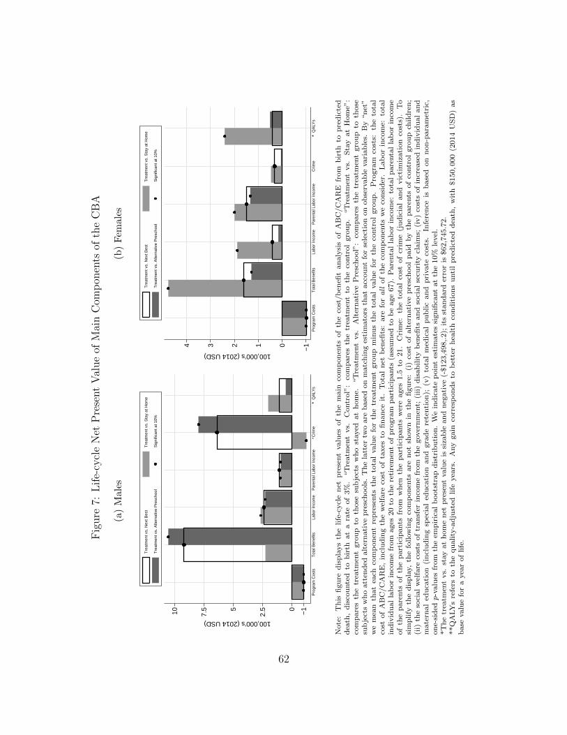
Fig
ure
7:L
ife-
cycl
eN
etP
rese
nt
Val
ue
ofM
ain
Com
pon
ents
ofth
eC
BA
(a)
Mal
es
−10
2.55
7.510
100,000’s (2014 USD)
Pro
gram
Cos
tsT
otal
Ben
efits
Labo
r In
com
eP
aren
tal L
abor
Inco
me
∗Crim
e∗∗
QA
LYs
Tre
atm
ent v
s. N
ext B
est
Tre
atm
ent v
s. S
tay
at H
ome
Tre
atm
ent v
s. A
ltern
ativ
e P
resc
hool
Sig
nific
ant a
t 10%
(b)
Fem
ales
−101234
100,000’s (2014 USD)
Pro
gram
Cos
tsT
otal
Ben
efits
Labo
r In
com
eP
aren
tal L
abor
Inco
me
Crim
e∗∗
QA
LYs
Tre
atm
ent v
s. N
ext B
est
Tre
atm
ent v
s. S
tay
at H
ome
Tre
atm
ent v
s. A
ltern
ativ
e P
resc
hool
Sig
nific
ant a
t 10%
Note
:T
his
figu
red
isp
lays
the
life
-cycl
en
etp
rese
nt
valu
esof
the
main
com
pon
ents
of
the
cost
/b
enefi
tan
aly
sis
of
AB
C/C
AR
Efr
om
bir
thto
pre
dic
ted
dea
th,
dis
cou
nte
dto
bir
that
ara
teof
3%
.“T
reatm
ent
vs.
Contr
ol”
:co
mp
are
sth
etr
eatm
ent
toth
eco
ntr
ol
gro
up
.“T
reatm
ent
vs.
Sta
yat
Hom
e”:
com
pare
sth
etr
eatm
ent
gro
up
toth
ose
sub
ject
sw
ho
stayed
at
hom
e.“T
reatm
ent
vs.
Alt
ern
ati
ve
Pre
sch
ool”
:co
mp
are
sth
etr
eatm
ent
gro
up
toth
ose
sub
ject
sw
ho
att
end
edalt
ern
ati
ve
pre
sch
ools
.T
he
latt
ertw
oare
base
don
matc
hin
ges
tim
ato
rsth
at
acc
ou
nt
for
sele
ctio
non
ob
serv
ab
levari
ab
les.
By
“n
et”
we
mea
nth
at
each
com
pon
ent
rep
rese
nts
the
tota
lvalu
efo
rth
etr
eatm
ent
gro
up
min
us
the
tota
lvalu
efo
rth
eco
ntr
ol
gro
up
.P
rogra
mco
sts:
the
tota
lco
stof
AB
C/C
AR
E,
incl
ud
ing
the
wel
fare
cost
of
taxes
tofi
nan
ceit
.T
ota
ln
etb
enefi
ts:
are
forall
of
the
com
pon
ents
we
con
sid
er.
Lab
or
inco
me:
tota
lin
div
idu
al
lab
or
inco
me
from
ages
20
toth
ere
tire
men
tof
pro
gra
mp
art
icip
ants
(ass
um
edto
be
age
67).
Pare
nta
lla
bor
inco
me:
tota
lp
are
nta
lla
bor
inco
me
of
the
pare
nts
of
the
part
icip
ants
from
wh
enth
ep
art
icip
ants
wer
eages
1.5
to21.
Cri
me:
the
tota
lco
stof
crim
e(j
ud
icia
lan
dvic
tim
izati
on
cost
s).
To
sim
plify
the
dis
pla
y,th
efo
llow
ing
com
pon
ents
are
not
show
nin
the
figu
re:
(i)
cost
of
alt
ern
ati
ve
pre
sch
ool
paid
by
the
pare
nts
of
contr
ol
gro
up
child
ren
;(i
i)th
eso
cial
wel
fare
cost
sof
tran
sfer
inco
me
from
the
gover
nm
ent;
(iii
)d
isab
ilit
yb
enefi
tsan
dso
cial
secu
rity
claim
s;(i
v)
cost
sof
incr
ease
din
div
idu
al
an
dm
ate
rnal
edu
cati
on
(in
clu
din
gsp
ecia
led
uca
tion
an
dgra
de
rete
nti
on
);(v
)to
tal
med
ical
pu
blic
an
dp
rivate
cost
s.In
fere
nce
isb
ase
don
non
-para
met
ric,
on
e-si
ded
p-v
alu
esfr
om
the
emp
iric
al
boots
trap
dis
trib
uti
on
.W
ein
dic
ate
poin
tes
tim
ate
ssi
gn
ifica
nt
at
the
10%
level
.*T
he
trea
tmen
tvs.
stay
at
hom
en
etp
rese
nt
valu
eis
siza
ble
an
dn
egati
ve
(-$123,4
98,.2);
its
stan
dard
erro
ris
$62,7
45.7
2.
**Q
ALY
sre
fers
toth
equ
ality
-ad
just
edlife
yea
rs.
Any
gain
corr
esp
on
ds
tob
ette
rh
ealt
hco
nd
itio
ns
unti
lp
red
icte
ddea
th,
wit
h$150,0
00
(2014
US
D)
as
base
valu
efo
ra
yea
rof
life
.
62

Females are less likely to work than males. While all males supply labor in our
sample at age 30, not all females do. We are not able to quantify household
production benefits for either males or females. This is an important omission
for females who decide to stay at home instead of work. For example, we lack
data on their children’s outcomes.
ABC/CARE has treatment effects on crime for females for a number of
categories (see Appendix G). However, males are much more likely to commit
crimes that are more costly to the victims, to the criminal justice system,
and to society (Cohen and Bowles, 2010; Barak et al., 2015). ABC/CARE
also has treatment effects on crime for females for a number of categories (see
Appendix G). However, males commit crimes that are much more expensive
to society. These two categories are examples of why the magnitudes of the
gains are much higher for males than they are for females.
For health, there are also substantial gender differences. Both males and
females have substantial gains: males benefit on more standard measures of
physical health, and females benefit on a set of mental health measures (see
Appendix G). We quantify both components (see Section 5.4 and Appendix F).
There is a second factor at work. There are substantial differences between
males and females in one counterfactual: treatment vs. alternative preschools.
The estimated treatment effects are very similar across genders for treatment
compared to those staying at home full time. Males benefit much more from
treatment relative to alternative preschools compared to their benefits from
treatment relative to staying at home. This result is consistent with find-
ings noted elsewhere: (i) stark gender differences resulting from attending low
63

quality childcare (Kottelenberg and Lehrer, 2014; Baker et al., 2015); and (ii)
females are less sensitive to uncertain environments (see, e.g., Autor et al.,
2015).
Our evidence does not indicate that the program has no benefits for fe-
males. When compared to staying at home, there is a gain of 4.93 dollars
per each dollar invested. When we decompose the net-present value for each
of the components that we monetize, we find substantial benefits for females
across a variety of categories, including health and crime. For males, the mag-
nitudes are noticeably increased when comparing outcomes from treatment to
outcomes from attending alternative preschools (see Figure 7).
7 Summary
This paper studies two influential early childhood programs evaluated by the
method of randomized control trials with long term follow-up through the mid
30’s. These programs are emulated in a variety of active early childhood pro-
grams around the world. We document outcomes across multiple life domains.
We estimate a statistically significant aggregate benefit/cost ratio of 7.3 and
a rate of return of 13.7% per annum, even after adjusting for the welfare costs
of financing the program through taxation.
To reach these conclusions, we address a number of empirical challenges:
(i) control group substitution; (ii) extrapolating lifetime benefits beyond the
experimental period; and (iii) the multiplicity of hypotheses tested. Our ap-
proach serves as a template for evaluations of programs with partial follow up
64

over the life cycle.
Benefits differ substantially by gender. Females have more beneficial treat-
ment effects than males, but the monetized value of the male treatment ef-
fects is greater. There are substantial effects on health and (health-related)
quality of life as well as crime for males. For females, the benefits are concen-
trated in education, employment, and minor crimes. The effects for females
are stronger compared to the alternative of staying at home. The effects for
males are stronger compared to the alternative of participation in alternative
childcare arrangements. The program subsidizes maternal employment and
has a strong causal effect on maternal labor income. We demonstrate the
long-term multiple benefits of these programs.
References
Autor, D. H., D. Figlio, K. Karbownik, J. Roth, and M. Wasserman (2015,October). Family disadvantage and the gender gap in behavioral and edu-cational outcomes. Working Paper WP-15-16, Institute for Policy Research,Northwestern University, Evanston, IL.
Baker, M., J. Gruber, and K. Milligan (2015, September). Non-cognitivedeficits and young adult outcomes: The long-run impacts of a universalchild care program. Working Paper 21571, National Bureau of EconomicResearch.
Barak, G., P. Leighton, and A. Cotton (2015). Class, Race, Gender, andCrime: The Social Realities of Justice in America. Rowman and Littlefield.
Barnett, W. S. and L. N. Masse (2002). A benefit-cost analysis of theAbecedarian Early Childhood Intervention. Technical report, National In-stitute for Early Education Research, New Brunswick, NJ.
65

Barnett, W. S. and L. N. Masse (2007, February). Comparative benefit-costanalysis of the Abecedarian program and its policy implications. Economicsof Education Review 26 (1), 113–125.
Belfield, C. R., M. Nores, W. S. Barnett, and L. J. Schweinhart (2006). TheHigh/Scope Perry Preschool Program: Cost-benefit analysis using data fromthe age-40 followup. Journal of Human Resources 41 (1), 162–190.
Blundell, R., M. Graber, and M. Mogstad (2015, July). Labor income dy-namics and the insurance from taxes, transfers, and the family. Journal ofPublic Economics 127, 58–73.
Burchinal, M. R., F. A. Campbell, D. M. Bryant, B. H. Wasik, and C. T.Ramey (1997, October). Early intervention and mediating processes incognitive performance of children of low-income African American families.Child Development 68 (5), 935–954.
Campbell, F. A., G. Conti, J. J. Heckman, S. H. Moon, R. Pinto, E. P. Pun-gello, and Y. Pan (2014). Early childhood investments substantially boostadult health. Science 343 (6178), 1478–1485.
Clarke, S. H. and F. A. Campbell (1998). Can intervention early preventcrime later? The Abecedarian Project compared with other programs. EarlyChildhood Research Quarterly 13 (2), 319–343.
Cohen, M. A. and R. Bowles (2010). Estimating costs of crime. In A. R.Piquero and D. Weisburd (Eds.), Handbook of Quantitative Criminology,Chapter 8, pp. 143–161. New York: Springer.
Collins, A., B. D. Goodson, J. Luallen, A. R. Fountain, A. Checkoway, andAbt Associates Inc. (2010, June). Evaluation of child care subsidy strategies:Massachusetts Family Child Care study. Technical Report OPRE 2011-1,Office of Planning, Research and Evaluation, Administration for Childrenand Families, U.S. Department of Health and Human Services, Washington,DC.
Currie, J. (2011). Inequality at birth: Some causes and consequences. Ameri-can Economic Review 101 (3), 1–22.
Department of Health, Education, and Welfare (1968). Federal interagency daycare requirements, pursuant to Sec. 522 (D) of the Economic OpportunityAct. Technical report, U.S. Department of Labor, Washington, DC.
66

Dolan, P. (1997). Modeling valuations for EuroQol health states. MedicalCare 35 (11), 1095–1108.
Duncan, G. J. and A. J. Sojourner (2013). Can intensive early childhoodintervention programs eliminate income-based cognitive and achievementgaps? Journal of Human Resources 48 (4), 945–968.
Educare (2014). A national research agenda for early education. Techni-cal report, Educare Learning Network Research & Evaluation Committee,Chicago, IL.
Elango, S., , J. L. Garcıa, J. J. Heckman, and A. Hojman (2016). Earlychildhood education. In R. A. Moffitt (Ed.), Economics of Means-TestedTransfer Programs in the United States, Volume 2, Chapter 4, pp. 235–297.Chicago: University of Chicago Press.
Feldstein, M. (1999, November). Tax avoidance and the deadweight loss of theincome tax. Review of Economics and Statistics 81 (4), 674–680.
Fox Business News (2014). Head Start has little effect by gradeschool? Video, http://video.foxbusiness.com/v/3306571481001/head-start-has-little-effect-by-grade-school/?#sp=show-clips.
Garcıa, J. L., J. J. Heckman, A. Hojman, Y. K. Koh, J. Shea, and A. Ziff(2016). Documentation of full ABC/CARE treatment effects. UnpublishedManuscript, University of Chicago.
Gladden, T. and C. Taber (2000). Wage progression among less skilled workers.In D. E. Card and R. M. Blank (Eds.), Finding Jobs: Work and WelfareReform, Chapter 4, pp. 160–192. New York: Russell Sage Foundation.
Goldman, D. P., D. Lakdawalla, P.-C. Michaud, C. Eibner, Y. Zheng, A. Gai-ley, I. Vaynman, J. Sullivan, B. Tysinger, and D. Ermini Leaf (2015). TheFuture Elderly Model: Technical documentation. Technical report, Univer-sity of Southern California.
Gross, R. T., D. Spiker, and C. W. Haynes (1997). Helping Low Birth Weight,Premature Babies: The Infant Health and Development Program. Stanford,CA: Stanford University Press.
Haavelmo, T. (1943, January). The statistical implications of a system ofsimultaneous equations. Econometrica 11 (1), 1–12.
67

Haskins, R. (1985, June). Public school aggression among children with vary-ing day-care experience. Child Development 56 (3), 689–703.
Healthy Child Manitoba (2015, April). Starting early, starting strong: A guidefor play-based early learning in Manitoba: Birth to six. Technical report,Healthy Child Manitoba, Winnipeg, Manitoba.
Heckman, J. J. (1992). Randomization and social policy evaluation. In C. F.Manski and I. Garfinkel (Eds.), Evaluating Welfare and Training Programs,Chapter 5, pp. 201–230. Cambridge, MA: Harvard University Press.
Heckman, J. J., N. Hohmann, J. Smith, and M. Khoo (2000, May). Substitu-tion and dropout bias in social experiments: A study of an influential socialexperiment. Quarterly Journal of Economics 115 (2), 651–694.
Heckman, J. J., H. Ichimura, J. Smith, and P. E. Todd (1998, September).Characterizing selection bias using experimental data. Econometrica 66 (5),1017–1098.
Heckman, J. J., L. J. Lochner, and P. E. Todd (2006). Earnings functions, ratesof return and treatment effects: The Mincer equation and beyond. In E. A.Hanushek and F. Welch (Eds.), Handbook of the Economics of Education,Volume 1, Chapter 7, pp. 307–458. Amsterdam: Elsevier.
Heckman, J. J., S. H. Moon, R. Pinto, P. A. Savelyev, and A. Q. Yavitz (2010a,August). Analyzing social experiments as implemented: A reexaminationof the evidence from the HighScope Perry Preschool Program. QuantitativeEconomics 1 (1), 1–46.
Heckman, J. J., S. H. Moon, R. Pinto, P. A. Savelyev, and A. Q. Yavitz (2010b,February). The rate of return to the HighScope Perry Preschool Program.Journal of Public Economics 94 (1–2), 114–128.
Heckman, J. J. and S. Navarro (2004, February). Using matching, instrumentalvariables, and control functions to estimate economic choice models. Reviewof Economics and Statistics 86 (1), 30–57.
Heckman, J. J. and R. Pinto (2015). Causal analysis after Haavelmo. Econo-metric Theory 31 (1), 115–151.
Heckman, J. J., R. Pinto, and P. A. Savelyev (2013, October). Understand-ing the mechanisms through which an influential early childhood programboosted adult outcomes. American Economic Review 103 (6), 2052–2086.
68

Heckman, J. J. and R. Robb (1985, October-November). Alternative meth-ods for evaluating the impact of interventions: An overview. Journal ofEconometrics 30 (1–2), 239–267.
Jarosch, G. (2016). Searching for job security and the consequences of job loss.Forthcoming, Econometrica.
Jensen, B. and M. Nielsen (2016). Abecedarian programme, within aninnovative implementation framework (APIIF). A pilot study. Website,http://pure.au.dk/portal/en/projects/abecedarian-programme-within-an-innovative-implementation-framework-apiif-a-pilot-study(8d4da9a9-f2ff-44db-87cc-1278d1e7006c).html (Accessed 8/1/2016).
Kline, P. and C. Walters (2016). Evaluating public programs with close sub-stitutes: The case of Head Start. Forthcoming, Quarterly Journal of Eco-nomics.
Kottelenberg, M. J. and S. F. Lehrer (2014, August). The gender effectsof universal child care in Canada: Much ado about boys? Unpublishedmanuscript, Department of Economics, Queen’s University.
Lagakos, D., B. Moll, T. Porzio, N. Qian, and T. Schoellman (2016). Life-cyclewage growth across countries. Forthcoming, Journal of Political Economy.
Lehmann, E. and J. P. Romano (2005, June). Generalizations of the familywiseerror rate. Annals of Statistics 33 (3), 1138–1154.
McCollister, K. E., M. T. French, and H. Fang (2010). The cost of crimeto society: New crime-specific estimates for policy and program evaluation.Drug and Alcohol Dependence 108 (1–2), 98–109.
Mincer, J. (1974). Schooling, Experience, and Earnings. New York: ColumbiaUniversity Press for National Bureau of Economic Research.
Murray, C. (2013). Giving Kids a Fair Chance, pp. 63–67. MIT Press.
North Carolina General Assembly (1971). Chapter 803, House bill 100. InNorth Carolina General Assembly 1971 Session, North Carolina. An Actto protect children through licensing of day-care facilities and other limitedregulation.
Prentice, R. L. (1989). Surrogate endpoints in clinical trials: Definition andoperational criteria. Statistics in Medicine 8 (4), 431–440.
69

Quandt, R. E. (1972, June). A new approach to estimating switching regres-sions. Journal of the American Statistical Association 67 (338), 306–310.
Ramey, C. T., D. M. Bryant, J. J. Sparling, and B. H. Wasik (1985). ProjectCARE: A comparison of two early intervention strategies to prevent retardeddevelopment. Topics in Early Childhood Special Education 5 (2), 12–25.
Ramey, C. T. and F. A. Campbell (1979, February). Compensatory educationfor disadvantaged children. The School Review 87 (2), 171–189.
Ramey, C. T., F. A. Campbell, M. Burchinal, M. L. Skinner, D. M. Gardner,and S. L. Ramey (2000). Persistent effects of early childhood education onhigh-risk children and their mothers. Applied Developmental Science 4 (1),2–14.
Ramey, C. T., A. M. Collier, J. J. Sparling, F. A. Loda, F. A. Campbell,D. A. Ingram, and N. W. Finkelstein (1976). The Carolina AbecedarianProject: A longitudinal and multidisciplinary approach to the preventionof developmental retardation. In T. Tjossem (Ed.), Intervention Strategiesfor High-Risk Infants and Young Children, pp. 629–655. Baltimore, MD:University Park Press.
Ramey, C. T. and R. Haskins (1981). The modification of intelligence throughearly experience. Intelligence 5 (1), 5–19.
Ramey, C. T., M. C. Holmberg, J. H. Sparling, and A. M. Collier (1977).An introduction to the Carolina Abecedarian Project. In B. M. Caldwelland D. J. Stedman (Eds.), Infant Education: A Guide for Helping Hand-icapped Children in the First Three Years, Chapter 7, pp. 101–121. NewYork: Walker and Company.
Ramey, C. T., G. D. McGinness, L. Cross, A. M. Collier, and S. Barrie-Blackley(1982). The Abecedarian approach to social competence: Cognitive andlinguistic intervention for disadvantaged preschoolers. In K. M. Borman(Ed.), The Social Life of Children in a Changing Society, Chapter 7, pp.145–174. Hillsdale, NJ: Lawrence Erlbaum Associates.
Ramey, C. T. and B. J. Smith (1977, January). Assessing the intellectualconsequences of early intervention with high-risk infants. American Journalof Mental Deficiency 81 (4), 318–324.
70

Ramey, C. T., J. J. Sparling, and S. L. Ramey (2012). Abecedarian: TheIdeas, the Approach, and the Findings (1 ed.). Los Altos, CA: SociometricsCorporation.
Ramey, S. L., C. T. Ramey, and R. G. Lanzi (2014). Interventions for stu-dents from impoverished environments. In J. T. Mascolo, V. C. Alfonso,and D. P. Flanagan (Eds.), Essentials of Planning, Selecting and TailoringInterventions for Unique Learners, pp. 415–48. Hoboken, NJ: John Wiley& Sons, Inc.
Ridder, G. and R. Moffitt (2007). The econometrics of data combination.In J. J. Heckman and E. E. Leamer (Eds.), Handbook of Econometrics,Volume 6B, pp. 5469–5547. Amsterdam: Elsevier.
Romano, J. P. and A. M. Shaikh (2006, August). Stepup procedures for controlof generalizations of the familywise error rate. Annals of Statistics 34 (4),1850–1873.
Romano, J. P. and M. Wolf (2016). Efficient computation of adjusted p-valuesfor resampling-based stepdown multiple testing. Statistics and ProbabilityLetters 113, 38–40.
Sanders, C. and C. Taber (2012, September). Life-cycle wage growth andheterogeneous human capital. Annual Review of Economics 4, 399–425.
Schneider, B. and S.-K. McDonald (Eds.) (2007). Scale-Up in Education,Volume 1: Ideas in Principle. Lanham, Maryland: Rowman & LittlefieldPublishers.
Schweinhart, L. J., J. Montie, Z. Xiang, W. S. Barnett, C. R. Belfield, andM. Nores (2005). Lifetime Effects: The High/Scope Perry Preschool StudyThrough Age 40, Volume 14 of Monographs of the HighScope EducationalResearch Foundation. Ypsilanti, MI: High/Scope Press.
Scull, J., J. Hattie, J. Page, J. Sparling, C. Tayler, A. King, V. Nossar,A. Piers-Blundell, and C. Ramey (2015). Building a bridge into preschoolin remote Northern Territory communities.
Shaw, J. W., J. A. Johnson, and S. J. Coons (2005). Us valuation of theEQ-5D health states: Development and testing of the D1 valuation model.Medical Care 43 (3), 203–220.
71

Sparling, J. (2010). Highlights of research findings from the Abecedarian stud-ies. Technical report, Teaching Strategies, Inc., Center on Health and Edu-cation, Georgetown University, and FPG Child Development Institute, Uni-versity of North Carolina at Chapel Hill, Bethesda, MD.
Sparling, J. and I. Lewis (1979). LearningGames for the First Three Years: AGuide to Parent/Child Play. New York: Walker and Company.
Sparling, J. and I. Lewis (1984). LearningGames for Threes and Fours. NewYork: Walker and Company.
Sparling, J. J. (1974). Synthesizing educational objectives for infant curricula.Annual Meeting of the American Educational Research Association.
Spiker, D., C. W. Haynes, and R. T. Gross (Eds.) (1997). Helping Low BirthWeight, Premature Babies: The Infant Health and Development Program.Redwood City, CA: Stanford University Press.
Tysinger, B., D. E. Leaf, and D. P. Goldman (2015). The Future AmericaModel: Technical Documentation. Technical report, Working Document.
Wasik, B. H., C. Ramey, D. M. Bryant, and J. J. Sparling (1990, December).A longitudinal study of two early intervention strategies: Project CARE.Child Development 61 (6), 1682–1696.
Weiland, C. and H. Yoshikawa (2013). Impacts of a prekindergarten programon children’s mathematics, language, literacy, executive function, and emo-tional skills. Child Development 84 (6), 2112–2130.
Whitehurst, G. J. (2014, April). Testimony given to the Health, Education,Labor, and Pensions Committee of the U.S. Senate.
Yazejian, N. and D. M. Bryant (2012). Educare implementation study find-ings. Technical report, Frank Porter Graham Child Development Institute,Chapel Hill, NC.
72