Digital Modulation inCommunications Systems –An Introduction

Application Note 1298

®

This application note introduces the concepts of digital modulation used inmany communications systems today. Emphasis is placed on explaining the tradeoffs that are made to optimize efficiencies in system design.

Most communications systems fall into one of three categories: bandwidthefficient, power efficient, or cost efficient. Bandwidth efficiency describesthe ability of a modulation scheme to accommodate data within a limitedbandwidth. Power efficiency describes the ability of the system to reliablysend information at the lowest practical power level. In most systems,there is a high priority on bandwidth efficiency. The parameter to be optimized depends on the demands of the particular system, as can be seen in the following two examples.

For designers of digital terrestrial microwave radios, their highest priorityis good bandwidth efficiency with low bit-error-rate. They have plenty ofpower available and are not concerned with power efficiency. They are not especially concerned with receiver cost or complexity because they donot have to build large numbers of them.

On the other hand, designers of hand-held cellular phones put a high priority on power efficiency because these phones need to run on a battery.Cost is also a high priority because cellular phones must be low-cost toencourage more users. Accordingly, these systems sacrifice some bandwidthefficiency to get power and cost efficiency.

Every time one of these efficiency parameters (bandwidth, power or cost) is increased, another one decreases, or becomes more complex or does notperform well in a poor environment. Cost is a dominant system priority.Low-cost radios will always be in demand. In the past, it was possible tomake a radio low-cost by sacrificing power and bandwidth efficiency. Thisis no longer possible. The radio spectrum is very valuable and operatorswho do not use the spectrum efficiently could lose their existing licenses orlose out in the competition for new ones. These are the tradeoffs that mustbe considered in digital RF communications design.

This application note covers

• the reasons for the move to digital modulation; • how information is modulated onto in-phase (I) and quadrature (Q)

signals; • different types of digital modulation;• filtering techniques to conserve bandwidth; • ways of looking at digitally modulated signals;• multiplexing techniques used to share the transmission channel;• how a digital transmitter and receiver work;• measurements on digital RF communications systems;• an overview table with key specifications for the major digital

communications systems; and • a glossary of terms used in digital RF communications.

These concepts form the building blocks of any communications system. If you understand the building blocks, then you will be able to understandhow any communications system, present or future, works.

2

Introduction

1. Why digital modulation?1.1 Trading off simplicity and bandwidth1.2 Industry trends

2. Using I/Q modulation (amplitude and phase control) to convey information

2.1 Transmitting information2.2 Signal characteristics that can be modified2.3 Polar display - magnitude and phase represented together2.4 Signal changes or modifications in polar form2.5 I/Q formats2.6 I and Q in a radio transmitter2.7 I and Q in a radio receiver2.8 Why use I and Q?

3. Digital Modulation types and relative efficiencies3.1 Applications3.1.1 Bit rate and symbol rate3.1.2 Spectrum (bandwidth) requirements3.1.3 Symbol clock3.2 Phase Shift Keying (PSK)3.3 Frequency Shift Keying (FSK)3.4 Minimum Shift Keying (MSK)3.5 Quadrature Amplitude Modulation (QAM)3.6 Theoretical bandwidth efficiency limits3.7 Spectral efficiency examples in practical radios3.8 I/Q offset modulation3.9 Differential modulation3.10 Constant amplitude modulation

4. Filtering4.1 Nyquist or raised cosine filter4.2 Transmitter-receiver matched filters4.3 Gaussian filter4.4 Filter bandwidth parameter alpha 4.5 Filter bandwidth effects4.6 Chebyshev equiripple FIR (finite impulse response) filter4.7 Spectral efficiency versus power consumption

5. Different ways of looking at a digitally modulated signal5.1 Power and frequency view5.2 Constellation diagrams5.3 Eye diagrams5.4 Trellis diagrams

6. Sharing the channel6.1 Multiplexing - frequency6.2 Multiplexing - time6.3 Multiplexing - code6.4 Multiplexing - geography6.5 Combining multiplexing modes6.6 Penetration versus efficiency

7. How digital transmitters and receivers work7.1 A digital communications transmitter7.2 A digital communications receiver

3

Table of contents

8. Measurements on digital RF communications systems8.1 Power measurements8.1.1 Adjacent Channel Power8.2 Frequency measurements8.2.1 Occupied bandwidth8.3 Timing measurements8.4 Modulation accuracy8.5 Understanding Error Vector Magnitude (EVM)8.6 Troubleshooting with error vector measurements8.7 Magnitude versus phase error8.8 I/Q phase error versus time8.9 Error Vector Magnitude versus time8.10 Error spectrum (EVM versus frequency)

9. Summary

10. Overview of communications systems

11. Glossary of terms

4

Table of contents

The move to digital modulation provides more information capacity,compatibility with digital data services, higher data security, better quality communications, and quicker system availability. Developers ofcommunications systems face these constraints:

• available bandwidth • permissible power • inherent noise level of the system

The RF spectrum must be shared, yet every day there are more users forthat spectrum as demand for communications services increases. Digitalmodulation schemes have greater capacity to convey large amounts ofinformation than analog modulation schemes.

1.1 Trading off simplicity and bandwidthThere is a fundamental tradeoff in communication systems. Simple hardware can be used in transmitters and receivers to communicate information. However, this uses a lot of spectrum which limits the numberof users. Alternatively, more complex transmitters and receivers can beused to transmit the same information over less bandwidth. The transitionto more and more spectrally efficient transmission techniques requiresmore and more complex hardware. Complex hardware is difficult to design,test, and build. This tradeoff exists whether communication is over air orwire, analog or digital.

5

1. Why digital modulation?

ComplexHardware Less Spectrum

SimpleHardware

SimpleHardware

Fi 1

ComplexHardware

More Spectrum

Figure 1.The FundamentalTrade-off

1.2 Industry trendsOver the past few years a major transition has occurred from simple analogAmplitude Modulation (AM) and Frequency/Phase Modulation (FM/PM) tonew digital modulation techniques. Examples of digital modulation include

• QPSK (Quadrature Phase Shift Keying) • FSK (Frequency Shift Keying)• MSK (Minimum Shift Keying)• QAM (Quadrature Amplitude Modulation)

Another layer of complexity in many new systems is multiplexing. Twoprincipal types of multiplexing (or “multiple access”) are TDMA (TimeDivision Multiple Access) and CDMA (Code Division Multiple Access).These are two different ways to add diversity to signals allowing differentsignals to be separated from one another.

6

QAM, FSK,QPSKVector Signals

AM, FMScalar Signals

TDMA, CDMATime-VariantSignals

Required Measurement Capability

Sign

al/S

yste

m C

ompl

exityFigure 2.

Trends in the Industry

2.1 Transmitting informationTo transmit a signal over the air, there are three main steps:

1. A pure carrier is generated at the transmitter. 2. The carrier is modulated with the information to be transmitted.

Any reliably detectable change in signal characteristics can carry information.

3. At the receiver the signal modifications or changes are detected and demodulated.

2.2 Signal characteristics that can be modifiedThere are only three characteristics of a signal that can be changed overtime: amplitude, phase or frequency. However, phase and frequency arejust different ways to view or measure the same signal change.

In AM, the amplitude of a high-frequency carrier signal is varied in proportion to the instantaneous amplitude of the modulating messagesignal.

Frequency Modulation (FM) is the most popular analog modulation technique used in mobile communications systems. In FM, the amplitudeof the modulating carrier is kept constant while its frequency is varied by the modulating message signal.

Amplitude and phase can be modulated simultaneously and separately, but this is difficult to generate, and especially difficult to detect. Instead, in practical systems the signal is separated into another set of independentcomponents: I (In-phase) and Q (Quadrature). These components areorthogonal and do not interfere with each other.

7

2. Using I/Q modulationto convey information.

Modify aSignal

"Modulate"

Detect the Modifications "Demodulate"

Any reliably detectable change insignal characteristics can carry information

Amplitude

Frequency

or

Phase

Both Amplitude

and Phase

Figure 3.TransmittingInformation...(Analog or Digital)

Figure 4.Signal Characteristicsto Modify

2.3 Polar display - magnitude and phase represented togetherA simple way to view amplitude and phase is with the polar diagram. Thecarrier becomes a frequency and phase reference and the signal is interpretedrelative to the carrier. The signal can be expressed in polar form as amagnitude and a phase. The phase is relative to a reference signal, the carrierin most communication systems. The magnitude is either an absolute orrelative value. Both are used in digital communication systems. Polardiagrams are the basis of many displays used in digital communications,although it is common to describe the signal vector by its rectangular coordinates of I (In-phase) and Q (Quadrature).

2.4 Signal changes or modifications in polar formThis figure shows different forms of modulation in polar form. Magnitude is represented as the distance from the center and phase is represented as the angle.

Amplitude modulation (AM) changes only the magnitude of the signal.Phase modulation (PM) changes only the phase of the signal. Amplitudeand phase modulation can be used together. Frequency modulation (FM)looks similar to phase modulation, though frequency is the controlledparameter, rather than relative phase.

8

Phase

Mag

0 deg

Phase

Mag

0 deg

Magnitude Change

Phase0 deg

Phase Change

Frequency Change Magnitude & Phase Change

0 deg

0 deg

Figure 5.Polar Display -Magnitude and PhaseRepresented Together

Figure 6.Signal Changes orModifications

One example of the difficulties in RF design can be illustrated with simple amplitude modulation. Generating AM with no associated angularmodulation should result in a straight line on a polar display. This lineshould run from the origin to some peak radius or amplitude value. In practice, however, the line is not straight. The amplitude modulation itselfoften can cause a small amount of unwanted phase modulation. The resultis a curved line. It could also be a loop if there is any hysteresis in thesystem transfer function. Some amount of this distortion is inevitable inany system where modulation causes amplitude changes. Therefore, thedegree of effective amplitude modulation in a system will affect somedistortion parameters.

2.5 I/Q formatsIn digital communications, modulation is often expressed in terms of I andQ. This is a rectangular representation of the polar diagram. On a polardiagram, the I axis lies on the zero degree phase reference, and the Q axisis rotated by 90 degrees. The signal vector’s projection onto the I axis is its“I” component and the projection onto the Q axis is its “Q” component.

9

{{ { 0 deg

"I"

"Q"

Q-Value

I-ValueProject signalto "I" and "Q" axes

Polar to Rectangular Conversion

Figure 7.“I-Q” Format

2.6 I and Q in a radio transmitterI/Q diagrams are particularly useful because they mirror the way most digital communications signals are created using an I/Q modulator. In thetransmitter, I and Q signals are mixed with the same local oscillator (LO).A 90 degree phase shifter is placed in one of the LO paths. Signals that areseparated by 90 degrees are also known as being orthogonal to each otheror in quadrature. Signals that are in quadrature do not interfere with each other. They are two independent components of the signal. Whenrecombined, they are summed to a composite output signal. There are two independent signals in I and Q that can be sent and received withsimple circuits. This simplifies the design of digital radios. The mainadvantage of I/Q modulation is the symmetric ease of combining independentsignal components into a single composite signal and later splitting such acomposite signal into its independent component parts.

2.7 I and Q in a radio receiverThe composite signal with magnitude and phase (or I and Q) informationarrives at the receiver input. The input signal is mixed with the local oscillator signal at the carrier frequency in two forms. One is at an arbitraryzero phase. The other has a 90 degree phase shift. The composite inputsignal (in terms of magnitude and phase) is thus broken into an in-phase,I, and a quadrature, Q, component. These two components of the signal are independent and orthogonal. One can be changed without affecting the other.Normally, information cannot be plotted in a polar format and reinterpretedas rectangular values without doing a polar-to-rectangular conversion.This conversion is exactly what is done by the in-phase and quadraturemixing processes in a digital radio. A local oscillator, phase shifter, and two mixers can perform the conversion accurately and efficiently.

10

90 deg Phase Shift

Local Osc.(Carrier Freq.)

Q

I

CompositeOutputSignal

Σ

Local Osc.(Carrier Freq.)

Quadrature Component

In-Phase Component

CompositeInputSignal

90 degPhase Shift

Figure 8.I and Q in a PracticalRadio Transmitter

Figure 9.I and Q in a RadioReceiver

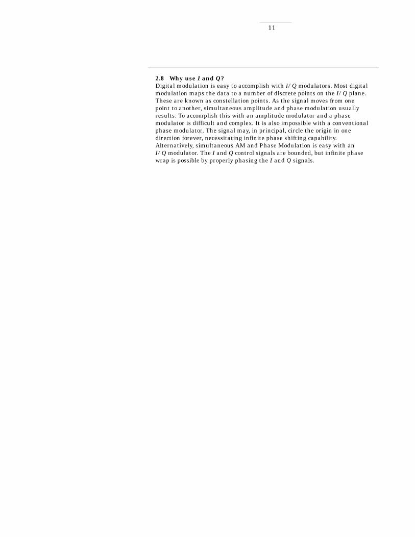
2.8 Why use I and Q?Digital modulation is easy to accomplish with I/Q modulators. Most digitalmodulation maps the data to a number of discrete points on the I/Q plane.These are known as constellation points. As the signal moves from onepoint to another, simultaneous amplitude and phase modulation usuallyresults. To accomplish this with an amplitude modulator and a phasemodulator is difficult and complex. It is also impossible with a conventionalphase modulator. The signal may, in principal, circle the origin in one direction forever, necessitating infinite phase shifting capability.Alternatively, simultaneous AM and Phase Modulation is easy with an I/Q modulator. The I and Q control signals are bounded, but infinite phase wrap is possible by properly phasing the I and Q signals.

11

This section covers the main digital modulation formats, their main applications, relative spectral efficiencies and some variations of the mainmodulation types as used in practical systems. Fortunately, there are alimited number of modulation types which form the building blocks of any system.

3.1 ApplicationsThis table covers the applications for different modulation formats in bothwireless communications and video.

Although this note focuses on wireless communications, video applicationshave also been included in the table for completeness and because of theirsimilarity to other wireless communications.

3.1.1 Bit rate and symbol rateTo understand and compare different modulation format efficiencies, it isimportant to first understand the difference between bit rate and symbolrate. The signal bandwidth for the communications channel needed dependson the symbol rate, not on the bit rate.

Symbol rate =bit rate

the number of bits transmitted with each symbol

12

3. Digital modulationtypes and relative efficiencies

Modulation format Application

MSK, GMSK GSM, CDPD

BPSK Deep space telemetry, cable modems

QPSK, π/4 DQPSK Satellite, CDMA, NADC, TETRA, PHS, PDC, LMDS, DVB-S, cable (returnpath), cable modems, TFTS

OQPSK CDMA, satellite

FSK, GFSK DECT, paging, RAM mobile data, AMPS, CT2, ERMES, land mobile, public safety

8, 16 VSB North American digital TV (ATV), broadcast, cable

8PSK Satellite, aircraft, telemetry pilots for monitoring broadband video systems

16 QAM Microwave digital radio, modems, DVB-C, DVB-T

32 QAM Terrestrial microwave, DVB-T

64 QAM DVB-C, modems, broadband set top boxes, MMDS

256 QAM Modems, DVB-C (Europe), Digital Video (US)

Bit rate is the frequency of a system bit stream. Take, for example, a radiowith an 8 bit sampler, sampling at 10 kHz for voice. The bit rate, the basicbit stream rate in the radio, would be eight bits multiplied by 10K samplesper second, or 80 Kbits per second. (For the moment we will ignore the extra bits required for synchronization, error correction, etc.).

Figure 10 is an example of a state diagram of a Quadrature Phase ShiftKeying (QPSK) signal. The states can be mapped to zeros and ones. This isa common mapping, but it is not the only one. Any mapping can be used.

The symbol rate is the bit rate divided by the number of bits that can betransmitted with each symbol. If one bit is transmitted per symbol, as withBPSK, then the symbol rate would be the same as the bit rate of 80 Kbitsper second. If two bits are transmitted per symbol, as in QPSK, then thesymbol rate would be half of the bit rate or 40 Kbits per second. Symbolrate is sometimes called baud rate. Note that baud rate is not the same asbit rate. These terms are often confused. If more bits can be sent with eachsymbol, then the same amount of data can be sent in a narrower spectrum.This is why modulation formats that are more complex and use a highernumber of states can send the same information over a narrower piece ofthe RF spectrum.

3.1.2 Spectrum (bandwidth) requirementsAn example of how symbol rate influences spectrum requirements can beseen in eight-state Phase Shift Keying (8PSK). It is a variation of PSK.There are eight possible states that the signal can transition to at anytime. The phase of the signal can take any of eight values at any symboltime. Since 23 = 8, there are three bits per symbol. This means the symbolrate is one third of the bit rate. This is relatively easy to decode.

13

01 00

1011

QPSKTwo Bits Per Symbol

QPSKState Diagram

BPSKOne Bit Per Symbol

Symbol Rate = Bit Rate

8PSKThree Bits Per Symbol

Symbol Rate = 1/3 Bit Rate

Figure 10.Bit Rate and SymbolRate

Figure 11.SpectrumRequirements

3.1.3 Symbol clockThe symbol clock represents the frequency and exact timing of the transmission of the individual symbols. At the symbol clock transitions, the transmitted carrier is at the correct I/Q (or magnitude/phase) value torepresent a specific symbol (a specific point in the constellation).

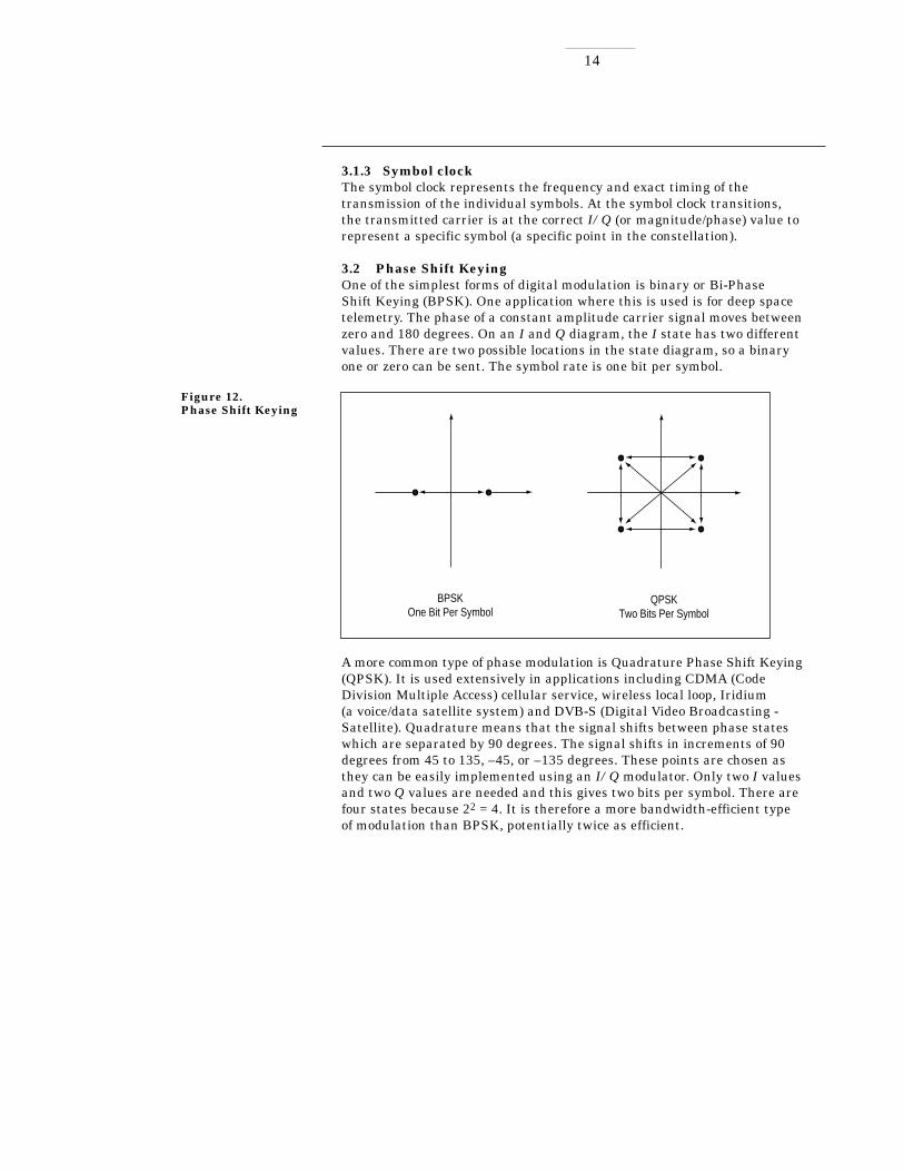
3.2 Phase Shift KeyingOne of the simplest forms of digital modulation is binary or Bi-Phase Shift Keying (BPSK). One application where this is used is for deep spacetelemetry. The phase of a constant amplitude carrier signal moves betweenzero and 180 degrees. On an I and Q diagram, the I state has two differentvalues. There are two possible locations in the state diagram, so a binaryone or zero can be sent. The symbol rate is one bit per symbol.

A more common type of phase modulation is Quadrature Phase Shift Keying(QPSK). It is used extensively in applications including CDMA (CodeDivision Multiple Access) cellular service, wireless local loop, Iridium (a voice/data satellite system) and DVB-S (Digital Video Broadcasting -Satellite). Quadrature means that the signal shifts between phase stateswhich are separated by 90 degrees. The signal shifts in increments of 90degrees from 45 to 135, –45, or –135 degrees. These points are chosen asthey can be easily implemented using an I/Q modulator. Only two I valuesand two Q values are needed and this gives two bits per symbol. There arefour states because 22 = 4. It is therefore a more bandwidth-efficient type of modulation than BPSK, potentially twice as efficient.

14

BPSKOne Bit Per Symbol

QPSKTwo Bits Per Symbol

Figure 12.Phase Shift Keying

3.3 Frequency Shift KeyingFrequency modulation and phase modulation are closely related. A staticfrequency shift of +1 Hz means that the phase is constantly advancing atthe rate of 360 degrees per second (2 π rad/sec), relative to the phase of theunshifted signal.

FSK (Frequency Shift Keying) is used in many applications including cordless and paging systems. Some of the cordless systems include DECT(Digital Enhanced Cordless Telephone) and CT2 (Cordless Telephone 2).

In FSK, the frequency of the carrier is changed as a function of the modulating signal (data) being transmitted. Amplitude remains unchanged.In binary FSK (BFSK or 2FSK), a “1” is represented by one frequency and a “0” is represented by another frequency.

3.4 Minimum Shift KeyingSince a frequency shift produces an advancing or retarding phase, frequencyshifts can be detected by sampling phase at each symbol period. Phaseshifts of (2N + 1) π/2 radians are easily detected with an I/Q demodulator.At even numbered symbols, the polarity of the I channel conveys the transmitted data, while at odd numbered symbols the polarity of the Qchannel conveys the data. This orthogonality between I and Q simplifiesdetection algorithms and hence reduces power consumption in a mobilereceiver. The minimum frequency shift which yields orthogonality of I and Qis that which results in a phase shift of ± π/2 radians per symbol (90 degreesper symbol). FSK with this deviation is called MSK (Minimum ShiftKeying). The deviation must be accurate in order to generate repeatable 90 degree phase shifts. MSK is used in the GSM (Global System for Mobile Communications) cellular standard. A phase shift of +90 degreesrepresents a data bit equal to “1”, while –90 degrees represents a “0”. Thepeak-to-peak frequency shift of an MSK signal is equal to one-half of the bit rate.

FSK and MSK produce constant envelope carrier signals, which have noamplitude variations. This is a desirable characteristic for improving thepower efficiency of transmitters. Amplitude variations can exercise nonlinearities in an amplifier’s amplitude-transfer function, generatingspectral regrowth, a component of adjacent channel power. Therefore, more efficient amplifiers (which tend to be less linear) can be used withconstant-envelope signals, reducing power consumption.

15

MSKQ vs. I

FSKFreq. vs. Time

One Bit Per Symbol One Bit Per Symbol

Figure 13.Frequency ShiftKeying

MSK has a narrower spectrum than wider deviation forms of FSK. Thewidth of the spectrum is also influenced by the waveforms causing thefrequency shift. If those waveforms have fast transitions or a high slew rate,then the spectrum of the transmitter will be broad. In practice, the waveforms are filtered with a Gaussian filter, resulting in a narrow spectrum. In addition, the Gaussian filter has no time-domain overshoot,which would broaden the spectrum by increasing the peak deviation. MSK with a Gaussian filter is termed GMSK (Gaussian MSK).

3.5 Quadrature Amplitude ModulationAnother member of the digital modulation family is Quadrature AmplitudeModulation (QAM). QAM is used in applications including microwave digital radio, DVB-C (Digital Video Broadcasting - Cable) and modems.

In 16-state Quadrature Amplitude Modulation (16QAM), there are four Ivalues and four Q values. This results in a total of 16 possible states for thesignal. It can transition from any state to any other state at every symboltime. Since 16 = 24, four bits per symbol can be sent. This consists of twobits for I and two bits for Q. The symbol rate is one fourth of the bit rate.So this modulation format produces a more spectrally efficient transmission.It is more efficient than BPSK, QPSK or 8PSK. Note that QPSK is thesame as 4QAM.

Another variation is 32QAM. In this case there are six I values and six Qvalues resulting in a total of 36 possible states (6x6=36). This is too manystates for a power of two (the closest power of two is 32). So the four cornersymbol states, which take the most power to transmit, are omitted. Thisreduces the amount of peak power the transmitter has to generate. Since25 = 32, there are five bits per symbol and the symbol rate is one fifth ofthe bit rate.

The current practical limits are approximately 256QAM, though work isunderway to extend the limits to 512 or 1024 QAM. A 256QAM systemuses 16 I-values and 16 Q-values giving 256 possible states. Since 28 = 256,each symbol can represent eight bits. A 256QAM signal that can send eight bits per symbol is very spectrally efficient. However, the symbols are very close together and are thus more subject to errors due to noise and distortion. Such a signal may have to be transmitted with extra power(to effectively spread the symbols out more) and this reduces power efficiency as compared to simpler schemes.

16

16QAMFour Bits Per Symbol

Symbol Rate = 1/4 Bit Rate

I

Q

32QAMFive Bits Per Symbol

Symbol Rate = 1/5 Bit Rate

Vector Diagram Constellation Diagram

Fig. 14

Figure 14.QuadratureAmplitude Modulation

Compare the bandwidth efficiency when using 256QAM versus BPSKmodulation in the radio example in section 3.1.1 (which uses an eight-bitsampler sampling at 10 kHz for voice). BPSK uses 80 Ksymbols-per-secondsending 1 bit per symbol. A system using 256QAM sends eight bits persymbol so the symbol rate would be 10 Ksymbols per second. A 256QAMsystem enables the same amount of information to be sent as BPSK usingonly one eighth of the bandwidth. It is eight times more bandwidth efficient. However, there is a tradeoff. The radio becomes more complex and is more susceptible to errors caused by noise and distortion. Error rates of higher-order QAM systems such as this degrade more rapidly thanQPSK as noise or interference is introduced. A measure of this degradationwould be a higher Bit Error Rate (BER).

In any digital modulation system, if the input signal is distorted or severe-ly attenuated the receiver will eventually lose symbol lock completely. Ifthe receiver can no longer recover the symbol clock, it cannot demodulatethe signal or recover any information. With less degradation, the symbolclock can be recovered, but it is noisy, and the symbol locations themselvesare noisy. In some cases, a symbol will fall far enough away from itsintended position that it will cross over to an adjacent position. The I andQ level detectors used in the demodulator would misinterpret such asymbol as being in the wrong location, causing bit errors. QPSK is not asefficient, but the states are much farther apart and the system can tolerate a lot more noise before suffering symbol errors. QPSK has nointermediate states between the four corner-symbol locations so there isless opportunity for the demodulator to misinterpret symbols. QPSKrequires less transmitter power than QAM to achieve the same bit errorrate.

3.6 Theoretical bandwidth efficiency limitsBandwidth efficiency describes how efficiently the allocated bandwidth isutilized or the ability of a modulation scheme to accommodate data, withina limited bandwidth. This table shows the theoretical bandwidth efficiencylimits for the main modulation types. Note that these figures cannot actually be achieved in practical radios since they require perfect modulators, demodulators, filter and transmission paths.

If the radio had a perfect (rectangular in the frequency domain) filter, thenthe occupied bandwidth could be made equal to the symbol rate.

Techniques for maximizing spectral efficiency include the following:

• Relate the data rate to the frequency shift (as in GSM).• Use premodulation filtering to reduce the occupied bandwidth.

Raised cosine filters, as used in NADC, PDC, and PHS give the best spectral efficiency.

• Restrict the types of transitions.

17

Modulation Theoretical bandwidth format efficiency limits

MSK 1 bit/second/Hz BPSK 1 bit/second/Hz QPSK 2 bits/second/Hz 8PSK 3 bits/second/Hz 16 QAM 4 bits/second/Hz 32 QAM 5 bits/second/Hz 64 QAM 6 bits/second/Hz 256 QAM 8 bits/second/Hz

3.7 Spectral efficiency examples in practical radiosThe following examples indicate spectral efficiencies that are achieved insome practical radio systems.

The TDMA version of the North American Digital Cellular (NADC) system,achieves a 48 Kbits-per-second data rate over a 30 kHz bandwidth or 1.6 bits per second per Hz. It is a π/4 DQPSK based system and transmitstwo bits per symbol. The theoretical efficiency would be two bits per secondper Hz and in practice it is 1.6 bits per second per Hz.

Another example is a microwave digital radio using 16QAM. This kind of signal is more susceptible to noise and distortion than somethingsimpler such as QPSK. This type of signal is usually sent over a direct line-of-sight microwave link or over a wire where there is very little noise andinterference. In this microwave-digital-radio example the bit rate is 140 Mbitsper second over a very wide bandwidth of 52.5 MHz. The spectral efficiencyis 2.7 bits per second per Hz. To implement this, it takes a very clear line-of-sight transmission path and a precise and optimized high-powertransceiver.

18

Effects of going through the originTake, for example, a QPSK signal wherethe normalized value changes from 1, 1to –1, –1. When changing simultaneous-ly from I and Q values of +1 to I and Qvalues of –1, the signal trajectory goesthrough the origin (the I/Q value of 0,0).The origin represents 0 carrier magni-tude. A value of 0 magnitude indicatesthat the carrier amplitude is 0 for amoment.

Not all transitions in QPSK result in atrajectory that goes through the origin.If I changes value but Q does not (orvice-versa) the carrier amplitude changes a little, but it does not gothrough zero. Therefore some symboltransitions will result in a small ampli-tude variation, while others will resultin a very large amplitude variation. Theclock-recovery circuit in the receivermust deal with this amplitude variationuncertainty if it uses amplitude varia-tions to align the receiver clock with thetransmitter clock.

Spectral regrowth does not automatical-ly result from these trajectories that passthrough or near the origin. If the ampli-fier and associated circuits are perfectlylinear, the spectrum (spectral occupancyor occupied bandwidth) will be un-changed. The problem lies in nonlinear-ities in the circuits.

A signal which changes amplitude overa very large range will exercise thesenonlinearities to the fullest extent. Thesenonlinearities will cause distortionproducts. In continuously-modulatedsystems they will cause “spectral re-growth” or wider modulation sidebands(a phenomenon related to intermodula-tion distortion). Another term which issometimes used in this context is “spec-tral splatter”. However this is a termthat is more correctly used in associa-tion with the increase in the bandwidthof a signal caused by pulsing on and off.

Digital modulation types - variations

The modulation types outlined in sections 3.2 to 3.4 form the building blocksfor many systems. There are three main variations on these basic buildingblocks that are used in communications systems: I/Q offset modulation,differential modulation, and constant envelope modulation.

3.8 I/Q offset modulationThe first variation is offset modulation. One example of this is OffsetQPSK (OQPSK). This is used in the cellular CDMA (Code DivisionMultiple Access) system for the reverse (mobile to base) link.

In QPSK, the I and Q bit streams are switched at the same time. Thesymbol clocks, or the I and Q digital signal clocks, are synchronized. InOffset QPSK (OQPSK), the I and Q bit streams are offset in their relativealignment by one bit period (one half of a symbol period). This is shown in the diagram. Since the transitions of I and Q are offset, at any giventime only one of the two bit streams can change values. This creates adramatically different constellation, even though there are still just twoI/Q values. This has power efficiency advantages. In OQPSK the signaltrajectories are modified by the symbol clock offset so that the carrieramplitude does not go through or near zero (the center of the constellation).The spectral efficiency is the same with two I states and two Q states. Thereduced amplitude variations (perhaps 3 dB for OQPSK, versus 30 to 40 dBfor QPSK) allow a more power-efficient, less linear RF power amplifier to be used.

19

QPSK

OffsetQPSK

Q

I

Q

I

Eye Constellation

Figure 15.I-Q “Offset”Modulation

3.9 Differential modulationThe second variation is differential modulation as used in differentialQPSK (DQPSK) and differential 16QAM (D16QAM). Differential meansthat the information is not carried by the absolute state, it is carried by the transition between states. In some cases there are also restrictions onallowable transitions. This occurs in π/4 DQPSK where the carrier trajectory does not go through the origin. A DQPSK transmission systemcan transition from any symbol position to any other symbol position. The π/4 DQPSK modulation format is widely used in many applicationsincluding

• cellular-NADC- IS-54 (North American digital cellular)-PDC (Pacific Digital Cellular)

• cordless -PHS (personal handyphone system)

• trunked radio-TETRA (Trans European Trunked Radio)

The π/4 DQPSK modulation format uses two QPSK constellations offset by 45 degrees (π/4 radians). Transitions must occur from one constellationto the other. This guarantees that there is always a change in phase at each symbol, making clock recovery easier. The data is encoded in themagnitude and direction of the phase shift, not in the absolute position on the constellation. One advantage of π/4 DQPSK is that the signal trajectory does not pass through the origin, thus simplifying transmitterdesign. Another is that π/4 DQPSK, with root raised cosine filtering, has better spectral efficiency than GMSK, the other common cellularmodulation type.

20

QPSK π/4 DQPSK

Both formats are 2 bits/symbol

Figure 16.“Differential”Modulation

3.10 Constant amplitude modulationThe third variation is constant-envelope modulation. GSM uses a variationof constant amplitude modulation format called 0.3 GMSK (GaussianMinimum Shift Keying).

In constant-envelope modulation the amplitude of the carrier is constant,regardless of the variation in the modulating signal. It is a power-efficientscheme that allows efficient class-C amplifiers to be used without introducing degradation in the spectral occupancy of the transmittedsignal. However, constant-envelope modulation techniques occupy a largerbandwidth than schemes which are linear. In linear schemes, the amplitudeof the transmitted signal varies with the modulating digital signal as inBPSK or QPSK. In systems where bandwidth efficiency is more importantthan power efficiency, constant envelope modulation is not as well suited.

MSK (covered in section 3.4) is a special type of FSK where the peak-to-peakfrequency deviation is equal to half the bit rate.

GMSK is a derivative of MSK where the bandwidth required is furtherreduced by passing the modulating waveform through a Gaussian filter.The Gaussian filter minimizes the instantaneous frequency variations overtime. GMSK is a spectrally efficient modulation scheme and is particularlyuseful in mobile radio systems. It has a constant envelope, spectral efficiency, good BER performance and is self-synchronizing.

21

MSK (GSM)

Amplitude (Envelope) VariesFrom Zero to Nominal Value

QPSK

Amplitude (Envelope) DoesNot Vary At All

Fig. 17

Figure 17.Constant AmplitudeModulation

Filtering allows the transmitted bandwidth to be significantly reducedwithout losing the content of the digital data. This improves the spectralefficiency of the signal.

There are many different varieties of filtering. The most common are

• raised cosine • square-root raised cosine• Gaussian filters

Any fast transition in a signal, whether it be amplitude, phase or frequency will require a wide occupied bandwidth. Any technique thathelps to slow down these transitions will narrow the occupied bandwidth.Filtering serves to smooth these transitions (in I and Q). Filtering reduces interference because it reduces the tendency of one signal or onetransmitter to interfere with another in a Frequency-Division-Multiple-Access (FDMA) system. On the receiver end, reduced bandwidth improvessensitivity because more noise and interference are rejected.

Some tradeoffs must be made. One is that some types of filtering cause the trajectory of the signal (the path of transitions between the states) toovershoot in many cases. This overshoot can occur in certain types of filterssuch as Nyquist. This overshoot path represents carrier power and phase.For the carrier to take on these values it requires more output power from the transmitter amplifiers. It requires more power than would benecessary to transmit the actual symbol itself. Carrier power cannot beclipped or limited (to reduce or eliminate the overshoot) without causingthe spectrum to spread out again. Since narrowing the spectral occupancywas the reason the filtering was inserted in the first place, it becomes avery fine balancing act.

Other tradeoffs are that filtering makes the radios more complex and canmake them larger, especially if performed in an analog fashion. Filteringcan also create Inter-Symbol Interference (ISI). This occurs when thesignal is filtered enough so that the symbols blur together and each symbolaffects those around it. This is determined by the time-domain response, or impulse response of the filter.

4.1 Nyquist or raised cosine filterThis graph shows the impulse or time-domain response of a raised cosinefilter, one class of Nyquist filter. Nyquist filters have the property thattheir impulse response rings at the symbol rate. The filter is chosen to ring,or have the impulse response of the filter cross through zero, at the symbolclock frequency.

22

4. Filtering

0

0.5

1

-10 -5 0 5 10

hi

ti

One symbol

Figure 18.Nyquit or RaisedCosine Filter

The time response of the filter goes through zero with a period that exactlycorresponds to the symbol spacing. Adjacent symbols do not interfere witheach other at the symbol times because the response equals zero at allsymbol times except the center (desired) one. Nyquist filters heavily filterthe signal without blurring the symbols together at the symbol times. This is important for transmitting information without errors caused byInter-Symbol Interference. Note that Inter-Symbol Interference does existat all times except the symbol (decision) times. Usually the filter is split,half being in the transmit path and half in the receiver path. In this caseroot Nyquist filters (commonly called root raised cosine) are used in eachpart, so that their combined response is that of a Nyquist filter.

4.2 Transmitter-receiver matched filtersSometimes filtering is desired at both the transmitter and receiver. Filteringin the transmitter reduces the adjacent-channel-power radiation of thetransmitter, and thus its potential for interfering with other transmitters.

Filtering at the receiver reduces the effects of broadband noise and alsointerference from other transmitters in nearby channels.

To get zero Inter-Symbol Interference (ISI), both filters are designed untilthe combined result of the filters and the rest of the system is a full Nyquistfilter. Potential differences can cause problems in manufacturing becausethe transmitter and receiver are often manufactured by different companies.The receiver may be a small hand-held model and the transmitter may be a large cellular base station. If the design is performed correctly the resultsare the best data rate, the most efficient radio, and reduced effects of interference and noise. This is why root-Nyquist filters are used inreceivers and transmitters as √ Nyquist x √ Nyquist = Nyquist. Matchedfilters are not used in Gaussian filtering.

4.3 Gaussian filterIn contrast, a GSM signal will have a small blurring of symbols on each of the four states because the Gaussian filter used in GSM does not havezero Inter-Symbol Interference. The phase states vary somewhat causing a blurring of the symbols as shown in figure 17. Wireless system architects must decide just how much of the Inter-Symbol Interference canbe tolerated in a system and combine that with noise and interference.

23

Actual Data

Root RaisedCosine Filter

DAC

Detected Bits

Root RaisedCosine Filter

Transmitter

ReceiverDemodulator

Modulator

Figure 19.Transmitter-ReceiverMatched Filters

Gaussian filters are used in GSM because of their advantages in carrierpower, occupied bandwidth and symbol-clock recovery. The Gaussian filteris a Gaussian shape in both the time and frequency domains, and it doesnot ring like the raised cosine filters do. Its effects in the time domain arerelatively short and each symbol interacts significantly (or causes ISI) withonly the preceding and succeeding symbols. This reduces the tendency forparticular sequences of symbols to interact which makes amplifiers easierto build and more efficient.

4.4 Filter bandwidth parameter alpha The sharpness of a raised cosine filter is described by alpha (α). Alphagives a direct measure of the occupied bandwidth of the system and iscalculated as

occupied bandwidth = symbol rate X (1 + α).

If the filter had a perfect (brick wall) characteristic with sharp transitionsand an alpha of zero, the occupied bandwidth would be

for α = 0, occupied bandwidth = symbol rate X (1 + 0) = symbol rate.

24

Hz

Ch1Spectrum

LogMag

10dB/div

GHz

0

0.2

0.4

0.6

0.8

1

0 0.2 0.4 0.6 0.8 1

α = 0.3

α = 0.5

α = 0

α = 1.0

Fs : Symbol Rate

Figure 20.Gaussian Filter

Figure 21.Filter BandwidthParameters “α”

In a perfect world, the occupied bandwidth would be the same as the symbolrate, but this is not practical. An alpha of zero is impossible to implement.

Alpha is sometimes called the “excess bandwidth factor” as it indicates theamount of occupied bandwidth that will be required in excess of the idealoccupied bandwidth (which would be the same as the symbol rate).

At the other extreme, take a broader filter with an alpha of one, which iseasier to implement. The occupied bandwidth will be

for α = 1, occupied bandwidth = symbol rate X (1 + 1) = 2 X symbol rate.

An alpha of one uses twice as much bandwidth as an alpha of zero. In practice, it is possible to implement an alpha below 0.2 and make good,compact, practical radios. Typical values range from 0.35 to 0.5, thoughsome video systems use an alpha as low as 0.11. The corresponding term fora Gaussian filter is BT (bandwidth time product). Occupied bandwidthcannot be stated in terms of BT because a Gaussian filter’s frequencyresponse does not go identically to zero, as does a raised cosine. Commonvalues for BT are 0.3 to 0.5.

4.5 Filter bandwidth effectsDifferent filter bandwidths show different effects. For example, look at aQPSK signal and examine how different values of alpha effect the vectordiagram. If the radio has no transmitter filter as shown on the left of thegraph, the transitions between states are instantaneous. No filteringmeans an alpha of infinity.

Transmitting this signal would require infinite bandwidth. The centerfigure is an example of a signal at an alpha of 0.75. The figure on the rightshows the signal at an alpha of 0.375. The filters with alphas of 0.75 and0.375 smooth the transitions and narrow the frequency spectrum required.

Different filter alphas also affect transmitted power. In the case of theunfiltered signal, with an alpha of infinity, the maximum or peak power ofthe carrier is the same as the nominal power at the symbol states. No extrapower is required due to the filtering.

25

QPSK Vector Diagrams

No Filtering α = 0.75 α = 0.375

Figure 22.Effect of DifferentFilter Bandwidth

Take an example of a π/4 DQPSK signal as used in NADC (IS-54). If analpha of 1.0 is used, the transitions between the states are more gradualthan for an alpha of infinity. Less power is needed to handle those transitions. Using an alpha of 0.5, the transmitted bandwidth decreasesfrom 2 times the symbol rate to 1.5 times the symbol rate. This results in a 25% improvement in occupied bandwidth. The smaller alpha takes more peak power because of the overshoot in the filter’s step response. This produces trajectories which loop beyond the outer limits of theconstellation.

At an alpha of 0.2, about the minimum of most radios today, there is a needfor significant excess power beyond that needed to transmit the symbolvalues themselves. A typical value of excess power needed at an alpha of0.2 for QPSK with Nyquist filtering would be approximately 5dB. This ismore than three times as much peak power because of the filter used tolimit the occupied bandwidth.

These principles apply to QPSK, offset QPSK, DQPSK, and the varieties of QAM such as 16QAM, 32QAM, 64QAM, and 256QAM. Not all signalswill behave in exactly the same way, and exceptions include FSK, MSK andany others with constant-envelope modulation. The power of these signalsis not affected by the filter shape.

4.6 Chebyshev equiripple FIR (finite impulse respone) filterA Chebyshev equiripple FIR (finite impulse response) filter is used forbaseband filtering in IS-95 CDMA. With a channel spacing of 1.25 MHzand a symbol rate of 1.2288 MHz in IS-95 CDMA, it is vital to reduce leakage to adjacent RF channels. This is accomplished by using a filterwith a very sharp shape factor using an alpha value of only 0.113. A FIRfilter means that the filter’s impulse response exists for only a finitenumber of samples. Equiripple means that there is a “rippled” magnitudefrequency-respone envelope of equal maxima and minima in the pass- andstopbands. This FIR filter uses a much lower order than a Nyquist filter toimplement the required shape factor. The IS-95 FIR filter does not havezero Inter Symbol Interference (ISI). However, ISI in CDMA is not asimportant as in other formats since the correlation of 64 chips at a time isused to make a symbol decision. This “coding gain” tends to average out theISI and minimize its effect.

26

Figure 23.Chebyshev EquirippleFIR Filter

4.7 Competing goals of spectral efficiency and power consumptionAs with any natural resource, it makes no sense to waste the RF spectrumby using channel bands that are too wide. Therefore narrower filters areused to reduce the occupied bandwidth of the transmission. Narrowerfilters with sufficient accuracy and repeatability are more difficult to build.Smaller values of alpha increase ISI because more symbols can contribute.This tightens the requirements on clock accuracy. These narrower filtersalso result in more overshoot and therefore more peak carrier power. Thepower amplifier must then accommodate the higher peak power withoutdistortion. The bigger amplifier causes more heat and electrical interferenceto be produced since the RF current in the power amplifier will interferewith other circuits. Larger, heavier batteries will be required. The alternative is to have shorter talk time and smaller batteries. Constantenvelope modulation, as used in GMSK, can use class-C amplifiers whichare the most efficient. In summary, spectral efficiency is highly desirable,but there are penalties in cost, size, weight, complexity, talk time, and reliability.

27

There are a number of different ways to view a signal. This simplifiedexample is an RF pager signal at a center frequency of 930.004 MHz. Thispager uses two-level FSK and the carrier shifts back and forth between twofrequencies that are 8 kHz apart (930.000 MHz and 930.008 MHz). Thisfrequency spacing is small in proportion to the center frequency of 930.004 MHz. This is shown in figure 24 (a). The difference in periodbetween a signal at 930 MHz and one at 930 MHz plus 8 kHz is very small.Even with a high performance oscilloscope, using the latest in high-speeddigital techniques, the change in period cannot be observed or measured.

In a pager receiver the signals are first downconverted to an IF or base-band frequency. In this example, the 930.004 MHz FSK-modulated signalis mixed with another signal at 930.002 MHz. The FSK modulation causesthe transmitted signal to switch between 930.000 MHz and 930.008 MHz. The result is a baseband signal that alternates between two frequencies, –2 kHZ and +6 kHz. The demodulated signal shifts between –2 kHz and +6 kHz. The difference can be easily detected.

This is sometimes referred to as “zoom” time or IF time. To be more specific,it is a band-converted signal at IF or baseband. IF time is important as it is how the signal looks in the IF portion of a receiver. This is how the IF ofthe radio detects the different bits that are present. The frequency domainrepresentation is shown in figure 24 (c). Most pagers use a two-level,Frequency-Shift-Keying (FSK) scheme. FSK is used in this instancebecause it is less affected by multipath propagation, attenuation and interference, common in urban environments. It is possible to demodulateit even deep inside modern steel/concrete buildings, where attenuation,noise and interference would otherwise make reliable demodulation difficult.

28

5. Different ways oflooking at a digitally-modulated signal timeand frequency domainview

Time-DomainBaseband

Time-Domain"Zoom"

Freq.-DomainNarrowband

24 (a)

24 (c)

24 (b)

8 kHz

Figure 24.Time and FrequencyDomain View

5.1 Power and frequency viewThere are many different ways of looking at a digitally-modulated signal.To examine how transmitters turn on and off, a power-versus-timemeasurement is very useful for examining the power level changes involvedin pulsed or bursted carriers. For example, very fast power changes willresult in frequency spreading or spectral regrowth. This is also known asfrequency “splatter”. Very slow power changes waste valuable transmittime, as the transmitter cannot send data when it is not fully on. Turningon too slowly can also cause high bit error rates at the beginning of theburst. In addition, peak and average power levels must be well understood,since asking for excessive power from an amplifier can lead to compressionor clipping. These phenomena distort the modulated signal and usuallylead to spectral regrowth as well.

5.2 Constellation diagramsAs discussed, the rectangular I/Q diagram is a polar diagram of magnitudeand phase. A two-dimensional diagram of the carrier magnitude and phase(a standard polar plot) can be represented differently by superimposingrectangular axes on the same data and interpreting the carrier in terms of in-phase (I) and quadrature-phase (Q) components. It would be possibleto perform AM and PM on a carrier at the same time and send data thisway; it is easier for circuit design and signal processing to generate anddetect a rectangular, linear set of values (one set for I and an independentset for Q).

The example shown is a π/4 Differential Quadrature Phase Shift Keying(π/4 DQPSK) signal as described in the North American Digital Cellular(NADC) TDMA standard. This example is a 157-symbol DQPSK burst.

29

Freq

uenc

y

Time

Ampl

itude

Time

Power vs.Time

Freq. vs.Time

DQPSK, 157 Symbolsand "Trajectory"

Constellation Diagram

DQPSK, 157 Symbol Constellation with Noise

Polar Diagram

Q

I

Figure 25.Power and FrequencyView

Figure 26.Constellation Diagram

The polar diagram shows several symbols at a time. That is, it shows the instantaneous value of the carrier at any point on the continuous line between and including symbol times, represented as I/Q or magnitude/phase values.

The constellation diagram shows a repetitive “snapshot” of that sameburst, with values shown only at the decision points. The constellationdiagram displays phase errors, as well as amplitude errors, at the decisionpoints. The transitions between the decision points affects transmittedbandwidth. This display shows the path the carrier is taking but does notexplicitly show errors at the decision points. Constellation diagramsprovide insight into varying power levels,the effects of filtering, andphenomena such as Inter-Symbol Interference.

The relationship between constellation points and bits per symbol is

M=2n where M = number of constellation points n = bits/symbolor n= log2 (M)

This holds when transitions are allowed from any constellation point toany other.

5.3 Eye diagramsAnother way to view a digitally modulated signal is with an eye diagram.Separate eye diagrams can be generated, one for the I-channel data andanother for the Q-channel data. Eye diagrams display I and Q magnitudeversus time in an infinite persistence mode, with retraces. The I and Qtransitions are shown separately and an “eye” (or eyes) is formed at thesymbol decision times. QPSK has four distinct I/Q states, one in each quadrant. There are only two levels for I and two levels for Q. This forms a single eye for each I and Q. Other schemes use more levels and createmore nodes in time through which the traces pass. The lower example is a16QAM signal which has four levels forming three distinct “eyes”. The eyeis open at each symbol. A “good” signal has wide open eyes with compactcrossover points.

30

I-Mag

Q

-Mag

Time

QPSK

16QAM

I-Mag

Time

Figure 27.I and Q Eye Diagrams

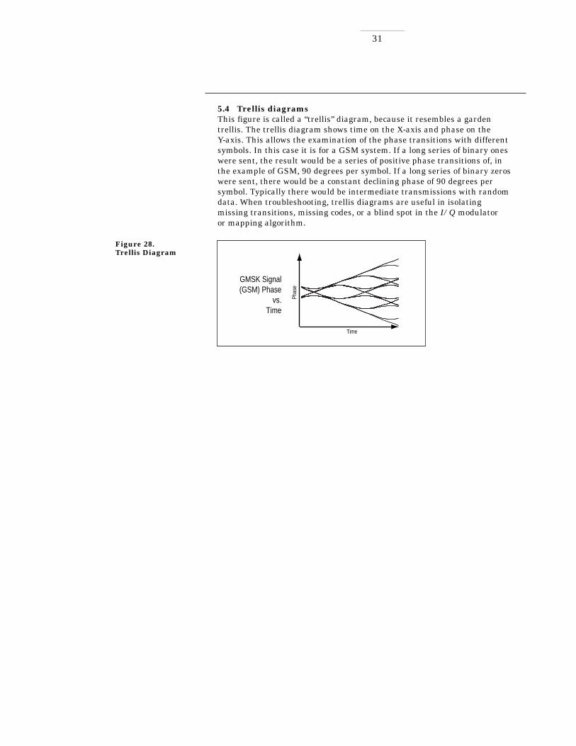
5.4 Trellis diagramsThis figure is called a “trellis” diagram, because it resembles a garden trellis. The trellis diagram shows time on the X-axis and phase on the Y-axis. This allows the examination of the phase transitions with differentsymbols. In this case it is for a GSM system. If a long series of binary oneswere sent, the result would be a series of positive phase transitions of, inthe example of GSM, 90 degrees per symbol. If a long series of binary zeroswere sent, there would be a constant declining phase of 90 degrees persymbol. Typically there would be intermediate transmissions with randomdata. When troubleshooting, trellis diagrams are useful in isolating missing transitions, missing codes, or a blind spot in the I/Q modulator or mapping algorithm.

31

Phas

e

Time

GMSK Signal(GSM) Phase

vs.Time

Figure 28.Trellis Diagram

The RF spectrum is a finite resource and is shared between users usingmultiplexing (sometimes called channelization). Multiplexing is used toseparate different users of the spectrum. This section covers multiplexingfrequency, time, code, and geography. Most communications systems use a combination of these multiplexing methods.

6.1 Multiplexing - frequencyFrequency Division Multiple-Access (FDMA) splits the available frequencyband into smaller fixed frequency channels. Each transmitter or receiveruses a separate frequency. This technique has been used since around 1900and is still in use today. Transmitters are narrowband or frequency-limited.A narrowband transmitter is used along with a receiver that has a narrow-band filter so that it can demodulate the desired signal and reject unwant-ed signals, such as interfering signals from adjacent radios.

6.2 Multiplexing - timeTime-division multiplexing involves separating the transmitters in time sothat they can share the same frequency. The simplest type is Time DivisionDuplex (TDD). This multiplexes the transmitter and receiver on the samefrequency. TDD is used, for example, in a simple two-way radio where abutton is pressed to talk and released to listen. This kind of time divisionduplex, however, is very slow. Modern digital radios like CT2 and DECTuse Time Division Duplex but they multiplex hundreds of times per second.TDMA (Time Division Multiple Access) multiplexes several transmitters orreceivers on the same frequency. TDMA is used in the GSM digital cellularsystem and also in the US NADC-TDMA system.

32

6. Sharing the channel

NarrowbandTransmitter

NarrowbandReceiver

TDMA Time Division Multiple-Access1

2

3

TDD Time Division Duplex

Am

plitu

de

Time

T R T R

A A A

B B BC C C

A B C

Figure 29.Multiplexing- Frequency

Figure 30.Multiplexing - Time

6.3 Multiplexing - codeCDMA is an access method where multiple users are permitted to transmitsimultaneously on the same frequency. Frequency division multiplexing isstill performed but the channel is 1.23 MHz wide. In the case of US CDMAtelephones, an additional type of channelization is added, in the form ofcoding.

In CDMA systems, users timeshare a higher-rate digital channel by overlaying a higher-rate digital sequence on their transmission. A differentsequence is assigned to each terminal so that the signals can be discernedfrom one another by correlating them with the overlaid sequence. This isbased on codes that are shared between the base and mobile stations.Because of the choice of coding used, there is a limit of 64 code channels on the forward link. The reverse link has no practical limit to the number of codes available.

6.4 Multiplexing - geographyAnother kind of multiplexing is geographical or cellular. If two transmitter/receiver pairs are far enough apart, they can operate on the same frequency and not interfere with each other. There are only a few kinds of systems that do not use some sort of geographic multiplexing.Clear-channel international broadcast stations, amateur stations, andsome military low frequency radios are about the only systems that haveno geographic boundaries and they broadcast around the world.

33

˜̃ Frequency

Amplitude

Time

F1

12

34

12

34

F1'

Figure 31.Multiplexing- Code

Figure 32.Multiplexing- Geography

6.5 Combining multiplexing modesIn most of these common communications systems, different forms of multiplexing are generally combined. For example, GSM uses FDMA,TDMA, FDD and geographic. DECT uses FDMA, TDD and geographicmultiplexing. For a full listing see the table in section ten.

6.6 Penetration versus efficiencyPenetration means the ability of a signal to be used in environments wherethere is a lot of attenuation or noise or interference. One very commonexample is the use of pagers versus cellular phones. In many cases, pagers can receive signals even if the user is inside a metal building or asteel-reinforced concrete structure like a modern skyscraper. Most pagersuse a two-level FSK signal where the frequency deviation is large and themodulation rate (symbol rate) is quite slow. This makes it easy for thereceiver to detect and demodulate the signal since the frequency differenceis large (the symbol locations are widely separated) and these differentfrequencies persist for a long time (a slow symbol rate).

However, the factors causing good pager signal penetration also cause inefficient information transmission. There are typically only two symbollocations. They are widely separated (approximately 8 kHz), and a smallnumber of symbols (500 to 1200) are sent each second. Compare this with a cellular system such as GSM which sends 270,833 symbols each second.This is not a big problem for the pager since all it needs to receive is itsunique address and perhaps a short ASCII text message.

A cellular phone signal, however, must transmit live duplex voice. Thisrequires a much higher bit rate and a much more efficient modulation technique. Cellular phones use more complex modulation formats (such as π/4 DQPSK and 0.3 GMSK) and faster symbol rates. Unfortunately, this greatly reduces penetration and one way to compensate is to use morepower. More power brings in a host of other problems, as described previously.

34

7.1 A digital communications transmitterHere is a simplified block diagram of a digital communications transmitter.It begins and ends with an analog signal. The first step is to convert acontinuous analog signal to a discrete digital bit stream. This is called digitization.

The next step is to add voice coding for data compression. Then some channel coding is added. Channel coding encodes the data in such a way as to minimize the effects of noise and interference in the communicationschannel. Channel coding adds extra bits to the input data stream andremoves redundant ones. Those extra bits are used for error correction orsometimes to send training sequences for identification or equalization.This can make synchronization (or finding the symbol clock) easier for thereceiver. The symbol clock represents the frequency and exact timing of the transmission of the individual symbols. At the symbol clock transitions,the transmitted carrier is at the correct I/Q (or magnitude/phase) value torepresent a specific symbol (a specific point in the constellation). Then thevalues (I/Q or magnitude/ phase) of the transmitted carrier are changed to represent another symbol. The interval between these two times is thesymbol clock period. The reciprocal of this is the symbol clock frequency.The symbol clock phase is correct when the symbol clock is aligned with the optimum instant(s) to detect the symbols.

The next step in the transmitter is filtering. Filtering is essential for good bandwidth efficiency. Without filtering, signals would have very fasttransitions between states and therefore very wide frequency spectra —much wider than is needed for the purpose of sending information. A singlefilter is shown for simplicity, but in reality there are two filters; one each for the I and Q channels. This creates a compact and spectrally efficientsignal that can be placed on a carrier.

The output from the channel coder is then fed into the modulator. Sincethere are independent I and Q components in the radio, half of the information can be sent on I and the other half on Q. This is one reasondigital radios work well with this type of digital signal. The I and Qcomponents are separate.

The rest of the transmitter looks similar to a typical RF transmitter ormicrowave transmitter/receiver pair. The signal is converted up to a higherintermediate frequency (IF), and then further upconverted to a higher radio frequency (RF). Any undesirable signals that were produced by theupconversion are then filtered out.

35

7. How digital transmitters andreceivers work

A/D

ModI I

Q Q

IF RF

Processing/Compression/Error Corr

EncodeSymbols

Figure 33.A Digital Transmitter

7.2 A digital communications receiverThe receiver is similar to the transmitter but in reverse. It is more complexto design. The incoming (RF) signal is first downconverted to (IF) anddemodulated. The ability to demodulate the signal is hampered by factorsincluding atmospheric noise, competing signals, and multipath or fading.

Generally, demodulation involves the following stages:

1. carrier frequency recovery (carrier lock)2. symbol clock recovery (symbol lock)3. signal decomposition to I and Q components4. determining I and Q values for each symbol (“slicing”)5. decoding and de-interleaving6. expansion to original bit stream7. digital-to-analog conversion, if required

In more and more systems, however, the signal starts out digital and staysdigital. It is never analog in the sense of a continuous analog signal likeaudio. The main difference between the transmitter and receiver is theissue of carrier and clock (or symbol) recovery.

Both the symbol-clock frequency and phase (or timing) must be correct in the receiver in order to demodulate the bits successfully and recover thetransmitted information. A symbol clock could be at the right frequencybut at the wrong phase. If the symbol clock was aligned with the transitionsbetween symbols rather than the symbols themselves, demodulation wouldbe unsuccessful.

Symbol clocks are usually fixed in frequency and this frequency is accuratelyknown by both the transmitter and receiver. The difficulty is to get themboth aligned in phase or timing. There are a variety of techniques and most systems employ two or more. If the signal amplitude varies duringmodulation, a receiver can measure the variations. The transmitter cansend a specific synchronization signal or a predetermined bit sequencesuch as 10101010101010 to “train” the receiver’s clock. In systems with apulsed carrier, the symbol clock can be aligned with the power turn-on ofthe carrier.

In the transmitter, it is known where the RF carrier and digital data clockare because they are being generated inside the transmitter itself. In thereceiver there is not this luxury. The receiver can approximate where thecarrier is but has no phase or timing symbol clock information. A difficulttask in receiver design is to create carrier and symbol-clock recovery algorithms. That task can be made easier by the channel coding performedin the transmitter.

36

AGC Demod QI I

QAdaption/Process/Decompress

D/A

IFRF

DecodeBits

Figure 34.A Digital Receiver

Complex tradeoffs in frequency, phase, timing, and modulation are made for interference-free, multiple-user communications systems. It isnecessary to accurately measure parameters in digital RF communicationssystems to make the right tradeoffs. Measurements include analyzing themodulator and demodulator, characterizing the transmitted signal quality,locating causes of high Bit-Error-Rate and investigating new modulationtypes. Measurements on digital RF communications systems generally fallinto four categories: power, frequency, timing, and modulation accuracy.

8.1 Power measurementsPower measurements include carrier power and associated measurementsof gain of amplifiers and insertion loss of filters and attenuators. Signalsused in digital modulation are noise-like. Band-power measurements(power integrated over a certain band of frequencies) or power spectraldensity (PSD) measurements are often made. PSD measurements normalize power to a certain bandwidth, usually 1 Hz.

8.1.1 Adjacent channel powerAdjacent channel power is a measure of interference created by one userthat effects other users in nearby channels. This test quantifies the energy of a digitally-modulated RF signal that spills from the intendedcommunication channel into an adjacent channel. The measurement resultis the ratio (in dB) of the power measured in the adjacent channel to thetotal transmitted power. A similar measurement is alternate channel power which looks at the same ratio two channels away from the intendedcommunication channel.

37

8. Measurements ondigital RF communicationssystems

TRACE A: Ch1 IQ Ref Time

A Ofs 38.500000 sym 3.43 dB 23.465 deg

100 uV

I-Q

20 uV/div

-100 uV

Ampl

itude

Frequency

GSM-TDMASignal

t

Figure 35.Power Measurement

Figure 36.Power and TimingMeasurements

For pulsed systems (such as TDMA), power measurements have a timecomponent and may have a frequency component, also. Burst power profile(power versus time) or turn-on and turn-off times may be measured.Another measurement is average power when the carrier is on or averagedover many on/off cycles.

8.2 Frequency measurementsFrequency measurements are often more complex in digital systems sincefactors other than pure tones must be considered. Occupied bandwidth is animportant measurement. It ensures that operators are staying within thebandwidth that they have been allocated. Adjacent channel power is alsoused to detect the effects one user has on other users in nearby channels.

8.2.1 Occupied bandwidthOccupied bandwidth (BW) is a measure of how much frequency spectrum is covered by the signal in question. The units are in Hz, and measurementof occupied BW generally implies a power percentage or ratio. Typically, a portion of the total power in a signal to be measured is specified. A common percentage used is 99%. A measurement of power versus frequency (such as integrated band power) is used to add up the power toreach the specified percentage. For example, one would say “99% of thepower in this signal is contained in a bandwidth of 30 kHz.” One could alsosay “The occupied bandwidth of this signal is 30 kHz” if the desired powerratio of 99% was known.

Typical occupied bandwidth numbers vary widely, depending on symbolrate and filtering. The figure is about 30 kHz for the NADC π/4 DQPSKsignal and about 350 kHz for a GSM 0.3 GMSK signal. For digital videosignals occupied bandwidth is typically 6 to 8 MHz.

Simple frequency-counter-measurement techniques are often not accurateor sufficient to measure center frequency. A carrier “centroid” can be calculated which is the center of the distribution of frequency versus PSDfor a modulated signal.

38

fo

Figure 37.FrequencyMeasurements

8.3 Timing measurementsTiming measurements are made most often in pulsed or burst systems.Measurements include pulse repetition intervals, on-time, off-time, dutycycle, and time between bit errors. Turn-on and turn-off times also involvepower measurements.

8.4 Modulation accuracyModulation accuracy measurements involve measuring how close either the constellation states or the signal trajectory is relative to a reference(ideal) signal trajectory. The received signal is demodulated and comparedwith a reference signal. The main signal is subtracted and what is left isthe difference or residual. Modulation accuracy is a residual measurement.

Modulation accuracy measurements usually involve precision demodulation of a signal and comparison of this demodulated signal with a (mathematically-generated) ideal or “reference” signal. The difference between the two is the modulation error, and it can be expressedin a variety of ways including Error Vector Magnitude (EVM), magnitudeerror, phase error, I-error and Q-error. The reference signal is subtractedfrom the demodulated signal, leaving a residual error signal. Residualmeasurements such as this are very powerful for troubleshooting. Once thereference signal has been subtracted, it is easier to see small errors thatmay have been swamped or obscured by the modulation itself. The errorsignal itself can be examined in many ways; in the time domain or (since itis a vector quantity) in terms of its I/Q or magnitude/phase components. A frequency transformation can also be performed and the spectral composition of the error signal alone can be viewed.

8.5 Understanding Error Vector MagnitudeRecall first the basics of vector modulation: Digital bits are transferred onto an RF carrier by varying the carrier’s magnitude and phase. At eachsymbol-clock transition, the carrier occupies any one of several unique locations on the I versus Q plane. Each location encodes a specific datasymbol, which consists of one or more data bits. A constellation diagramshows the valid locations (i.e., the magnitude and phase relative to thecarrier) for all permitted symbols of which there must be 2n, given n bitstransmitted per symbol. To demodulate the incoming data, the exact magnitude and phase of the received signal for each clock transition mustbe accurately determined.

The layout of the constellation diagram and its ideal symbol locations isdetermined generically by the modulation format chosen (BPSK, 16QAM,π/4 DQPSK, etc.). The trajectory taken by the signal from one symbol location to another is a function of the specific system implementation, but is readily calculated nonetheless.

At any moment, the signal’s magnitude and phase can be measured. These values define the actual or “measured” phasor. At the same time, acorresponding ideal or “reference” phasor can be calculated, given knowledgeof the transmitted data stream, the symbol-clock timing, baseband filteringparameters, etc. The differences between these two phasors form the basis for the EVM measurements.

39

Figure 38 defines EVM and several related terms. As shown, EVM is thescalar distance between the two phasor end points, i.e. it is the magnitudeof the difference vector. Expressed another way, it is the residual noise and distortion remaining after an ideal version of the signal has beenstripped away.

In the NADC-TDMA (IS-54) standard, EVM is defined as a percentage ofthe signal voltage at the symbols. In the π/4 DQPSK modulation format,these symbols all have the same voltage level, though this is not true of all formats. IS-54 is currently the only standard that explicitly definesEVM, so EVM could be defined differently for other modulation formats.

In a format such as 64QAM, for example, the symbols represent a varietyof voltage levels. EVM could be defined by the average voltage level of allthe symbols (a value close to the average signal level) or by the voltage ofthe outermost (highest voltage) four symbols. While the error vector has aphase value associated with it, this angle generally turns out to be randombecause it is a function of both the error itself (which may or may not berandom) and the position of the data symbol on the constellation (which,for all practical purposes, is random). A more useful angle is measuredbetween the actual and ideal phasors (I/Q phase error), which containsinformation useful in troubleshooting signal problems. Likewise, I-Qmagnitude error shows the magnitude difference between the actual andideal signals. EVM, as specified in the standard, is the root-mean-square(RMS) value of the error values at the instant of the symbol-clock transition. Trajectory errors between symbols are ignored.

8.6 Troubleshooting with error vector measurementsMeasurements of error vector magnitude and related quantities can, when properly applied, provide much insight into the quality of a digitallymodulated signal. They can also pinpoint the causes for any problemsuncovered by identifying exactly the type of degradation present in a signal and even help identify their sources. For more detail on using error-vector-magnitude measurements to analyze and troubleshoot vector-modulated signals, see product note 89400-14. The Hewlett-Packardliterature number is 5965-2898E.

40

{

I

QMagnitude Error (IQ error mag)

Error Vector

Ideal (Reference) Signal

Phase Error (IQ error phase)

MeasuredSignal

φ

Figure 38.EVM and RelatedQuantities

EVM measurements are growing rapidly in acceptance, having alreadybeen written into such important system standards as NADC and PHS, andthey are poised to appear in several upcoming standards including thosefor digital video transmission.

8.7 Magnitude versus phase errorDifferent error mechanisms affect signals in different ways: in magnitudeonly, phase only, or both simultaneously. Knowing the relative amounts ofeach type of error can quickly confirm or rule out certain types of problems.Thus, the first diagnostic step is to resolve EVM into its magnitude andphase error components (see figure 38) and compare their relative sizes.

When the average phase error (in degrees) is substantially larger than the average magnitude error (in percent), some sort of unwantedphase modulation is the dominant error mode. This could be caused bynoise, spurious or cross-coupling problems in the frequency reference,phase-locked loops, or other frequency-generating stages. Residual AM isevidenced by magnitude errors that are significantly larger than the phase angle errors.

8.8 I/Q phase error versus timePhase error is the instantaneous angle difference between the measuredsignal and the ideal reference signal. When viewed as a function of time(or symbol), it shows the modulating waveform of any residual or interfering PM signal. Sinewaves or other regular waveforms indicate an interferingsignal. Uniform noise is a sign of some form of phase noise (random jitter,residual PM/FM, etc.).

41

5deg

Phase

–5

99 Sym 0 Sym

MSK1 Phs Error 1

Figure 39.Incidental (inband)PM sinewave is clearly visible even atonly three degreespeak-to-peak.

A perfect signal will have a uniform constellation that is perfectly symmetricabout the origin. I/Q imbalance is indicated when the constellation is not“square”, i.e. when the Q-axis height does not equal the I-axis width.Quadrature error is seen in any “tilt” to the constellation. Quadrature error is caused when the phase relationship between the I and Q vectors is not exactly 90 degrees.

8.9 Error Vector Magnitude versus timeEVM is the difference between the input signal and the internally-generatedideal reference. When viewed as a function of symbol or time, errors may be correlated to specific points on the input waveform, such as peaks or zero crossings. EVM is a scalar (magnitude-only) value. Error peaksoccurring with signal peaks indicate compression or clipping. Error peaksthat correlate to signal minima suggest zero-crossing nonlinearities.

An example of zero-crossing nonlinearities is in a push-pull amplifier,where the positive and negative halves of the signal are handled by separate transistors. It can be quite a challenge (especially in high-poweramplifiers) to precisely bias and stabilize the amplifiers such that one setis turning off exactly as the other set is turning on, with no discontinuities.The critical moment is zero crossing, a well-known effect in analog design.It is also known as zero-crossing errors, distortion, or nonlinearities.

42

5deg

Real

–5

0 Sym 99 Sym

16QAM Phs Error 1

3%

Magnitude0

2

Magnitude

0

32QAM Err V Tim 1

40 Sym 80 Sym

32QAM Meas Time 1

40 Sym 80 Sym

Figure 40.Phase noise appearsrandom in the timedomain.

Figure 41.EVM peaks on thissignal (upper trace)occur every time thesignal magnitude(lower trace)approaches zero.This is probably azero-crossing errorin an amplificationstage.

8.10 Error spectrum (EVM versus frequency)The error spectrum is calculated from the Fast Fourier Transform (FFT) of the EVM waveform and results in a frequency-domain display that can show details not visible in the time domain. In most digital systems,nonuniform noise distribution or discrete signal peaks indicate the presence of externally-coupled interference.

For more detail on EVM measurements, see product note 89400-14 “Using Error-Vector-Magnitude Measurements to Analyze and TroubleshootVector-Modulated Signals.” The Hewlett-Packard literature number is5965-2898E.

43

30

dB%

rms

Mag (dB)

-120

825.962 MHz 826.038 MHz

PI/4 Err V Spec 1

30

dB%

rms

Mag (dB)

-120

825.962 MHz 826.038 MHz

PI/4 Err V Spec 1

Figure 42.Interference fromadjacent (lower)channel causesuneven EVM spectraldistribution.

Figure 43.Switching-power-supply interferenceappears as EVMspur, offset fromcarrier by 10kHz.

Communication system design requires the simultaneous conservation ofbandwidth, power, and cost. In the past, it was possible to make a radio low cost by sacrificing parameters such as power and bandwidth efficiency.

This application note has presented the building blocks of any communications system. With these concepts, you will be able to understand how communications systems work, and make more informeddecisions regarding the tradeoffs required to optimize your system.

9. Summary

GSM900 NADC PDC CDMA

Geography Europe North America Japan North America,Korea, Japan

Introduction 1992 1992 1993-1994 1995-1997

Frequency Range 935-960 MHz down 869-894 MHz down 810-826 MHz down 824-849 MHz (US) 890-915 MHz up 824-849 MHz up 940-956 MHz up 869-894 MHz (US) EGSM 925-960 MHz 1777-1801 MHz down 832-834, 843-846,

880-915 MHz 1429-1453 MHz up 860-870 MHz (Japan) 887-889, 898-901, 915-925 MHz (Japan)

Data Structure TDMA TDMA TDMA CDMA

Channel per 8-16 3-6 3-6 32-64 (Dyn. adapt) Frequency

Modulation 0.3 GMSK π/4 DQPSK π/4 DQPSK Mobile: QPSK(1 bit/symbol) (2 bits/symbol) (2 bits/symbol) Base: OQPSK

(1 bit/symbol)

Speech CODEC RELP-LTP VSELP 8 Kbits/s VSELP 8 Kbits/s 8 Kbits/s var rate CELP 13 Kbits/s EFR 13 kbit/s var rate CELP

Mobile Output 3.7mW to 20W 2.2mW to 6W .3W to 3W 10nW to 1W Power

Modulation 270.833 Kbits/s 48.6 Kbits/s 42 Kbits/s 9600/14,400 bps data; Data Rate (1 bit/symbol) (2 bits/symbol) (2 bits/symbol) 1.2288 Mb/s spreading

Filter 0.3 Gaussian SQRT raised cosine SQRT raised cosine Chebychev low α = .35 α = .50 pass (FIR)

Channel Spacing 200 kHz 30 kHz 50 kHz 1.23 MHz 25 kHz interleave

Number of 124 frequency ch. 832 frequency ch. 1600 frequency ch. 19-20 frequencies Channels w/8 timeslots per ch. w/3 users per ch. w/3 users per ch.

(1000) (2496) (4800)

Est # of 15-20 million 35-40 million 5 million Subscribers by (8.9 million 9/92) year 2000

Source GSM Standard IS-54 RCR Spec IS-95 specStd 27B

Service Public Cellular Public Cellular Public Cellular Public Cellular

4410. Overview of communicationssystems

DCS1800 PHS DECT TETRA Trans European Trunked Radio

Geography Europe Japan/China Europe/China Europe

Introduction 1993 1993 Private office 1993 19951995 Public

Frequency Range 1.7-1.9 GHz 1895-1918 MHz 1.897-1.913 GHz 450 MHz 1710-1785 MHz down up/down < 1 GHz1805-1880 MHz up 1.9, 1.93 GHz (China) 1.9, 1.93 GHz (China)

Data Structure TDMA TDMA/TDD TDMA/TDD TDMA

Channel per 8-16 4-8 12 4 Frequency

Modulation 0.3 GMSK π/4 DQPSK 0.5 GFSK π/4 DQPSK(1 bit/symbol) (2 bits/symbol) ±202-403 kHz dev

(1 bit/symbol)

Speech CODEC RELP-LTP ADPCM ADPCM Includes channel 13 Kbits/s 32 Kbits/s 32 Kbits/s & speech coding

7.2 Kbits/s

Mobile Output 250mW to 2W 10mW 250mWPower

Modulation Data 270.833 Kbits/s 384 Kbits/s 1.152 Mbit/s 19.2 Kb/s Rate

Filter 0.3 Gaussian SQRT raised cosine 0.5 Gaussian α = 0.4 SQRT α = .50 raised cosine

Channel Spacing 200 kHz 300 kHz 1.728 MHz 25 kHz

Number of 3000-6000 10 carrier frequencies Channels w/12 users per

frequency (120)

Est # of Subscribers 4-13 million 6.5-13 million by year 2000

Source prI-ETS 30 176 RCR spec Std 28 CI Spec., Part 1, Mobile Europe prETS 300 175-2 China-First News Rev 05.2e Magazine 1/92

Release 8/15/96 China-First News Release 8/15/96

Service Personal Cordless Telephone Wireless PBX Trunked system Communications Personal Adj. ch. sel > 60 dB

Communications

4510. Overview of communicationssystems

ACP Adjacent Channel PowerADPCM Adaptive Digital Pulse Code ModulationAM Amplitude ModulationAMPS Advanced Mobile Phone System

B-CDMA Broadband Code Division Multiple AccessBER Bit Error RateBPSK Binary Phase Shift KeyingBFSK Binary Frequency Shift KeyingBW Bandwidth

CDMA Code Division Multiple AccessCDPD Cellular Digital Packet DataCOFDM Coded Orthogonal Frequency Division MultiplexingCRC Cyclic Redundancy CheckCT2 Cordless Telephone - 2

DAB Digital Audio BroadcastDCS 1800 Digital Communication System - 1800 MHzDECT Digital Enhanced Cordless TelephoneDMCA Digital MultiChannel Access, similar to iDENDQPSK Differential Quadrature Phase Shift KeyingDSP Digital Signal ProcessingDVB-C Digital Video Broadcast - CableDVB-S Digital Video Broadcast - SatelliteDVB-T Digital Video Broadcast - Terrestrial

EGSM Extended Frequency GSMERMES European Radio Message SystemETSI European Telecommunications Standards InstituteEVM Error Vector Magnitude

FDD Frequency Division DuplexFDMA Frequency Division Multiple AccessFER Frame Error RateFFSK Fast Frequency Shift KeyingFFT Fast Fourier TransformFLEX 4-level FSK-based paging standard developed by

MotorolaFM Frequency ModulationFSK Frequency Shift Keying

GFSK Gaussian Frequency Shift Keying Globalstar Satellite system using 48 low-earth orbiting

satellitesGSM Global System for Mobile CommunicationGMSK Gaussian Minimum Shift Keying

HDTV High Definition Television

iDEN integrated Dispatch Enhanced Network (Motorola designed system for dispatch, cellular and conference calling)

46

11. Glossary of terms

IF Intermediate FrequencyI/Q In phase / QuadratureIridium Motorola voice/data 66-satellite system worldwideISI Intersymbol InterferenceIS-54 Interim Standard for US Digital Cellular (NADC)IS-95 Interim Standard for US Code Division Multiple

AccessIS-136 Interim Standard for NADC with Digital Control

Channels

LMDS Local Multipoint Distribution System

MFSK Minimum Frequency Shift KeyingMMDS Multichannel Multipoint Distribution SystemMPSK Minimum Phase Shift Keying

MSK Minimum Shift Keying

NADC North American Digital Cellular system

OFDM Orthogonal Frequency Division MultiplexingOQPSK Offset Quadrature Phase Shift Keying

PACS Personal Access Communications ServicePCS Personal Communications SystemPCM Pulse Code ModulationPDC Pacific Digital Cellular System (formerly JDC)PHS Personal Handyphone System (formerly PHP)PRBS Pseudo-Random Bit SequencePSD Power Spectral DensityPSK Phase Shift Keying

QAM Quadrature Amplitude ModulationQPSK Quadrature Phase Shift Keying

RAM Wireless data networkRF Radio FrequencyRMS Root Mean Square

SQRT Square Root

TDD Time Division DuplexTDMA Time Division Multiple AccessTETRA Trans European Trunked RadioTFTS Terrestrial Flight Telephone System

VSB Vestigal Side BandWLL Wireless Local Loop

47

11. Glossary of terms(cont’d)

For more information aboutHewlett-Packard test and measure-ment products, applications,services, and for a current salesoffice listing, visit our web site,http://www.hp.com/go/tmdir. Youcan also contact one of the followingcenters and ask for a test andmeasurement sales representative.

United States:Hewlett-Packard CompanyTest and Measurement Call CenterP.O. Box 4026Englewood, CO 80155-40261 800 452 4844

Canada:Hewlett-Packard Canada Ltd.5150 Spectrum WayMississauga, Ontario L4W 5G1(905) 206 4725

Europe:Hewlett-PackardEuropean Marketing CentreP.O. Box 9991180 AZ AmstelveenThe Netherlands(31 20) 547 9900

Japan:Hewlett-Packard Japan Ltd.Measurement Assistance Center9-1, Takakura-Cho, Hachioji-Shi,Tokyo 192, JapanTel: (81) 426-56-7832Fax: (81) 426-56-7840

Latin America:Hewlett-PackardLatin American Region Headquarters5200 Blue Lagoon Drive, 9th FloorMiami, Florida 33126, U.S.A.(305) 267 4245/4220

Australia/New Zealand:Hewlett-Packard Australia Ltd.31-41 Joseph StreetBlackburn, Victoria 3130, Australia1 800 629 485

Asia Pacific: Hewlett-Packard Asia Pacific Ltd.17-21/F Shell Tower, Times Square,1 Matheson Street, Causeway Bay,Hong KongTel: (852) 2599 7777Fax: (852) 2506 9285

Data Subject to ChangeCopyright © 1997Hewlett-Packard CompanyPrinted in U.S.A. 7/975965-7160E

®