diplomarbeit rpl ready to use: an embeddable and harald …
TRANSCRIPT

INSTITUT FÜR INFORMATIKDER LUDWIG–MAXIMILIANS–UNIVERSITÄT MÜNCHEN
Diplomarbeit
RPL ready to use: An embeddable andexpressive, yet efficient RDF Path Language
Harald Zauner
aufgabensteller Prof. Dr. François Bry
betreuer Dr. Benedikt LinseDr. Tim Furche
abgabetermin 14. März 2010


E R K L Ä R U N G
Hiermit versichere ich, dass ich die vorliegende Diplomarbeit selbstständigverfasst und keine anderen als die angegebenen Quellen und Hilfsmittelverwendet habe.
München, 14. März 2010
Harald Zauner

A B S T R A C T
SPARQL is so far the only standardized RDF query language. Surprisingly, itis designed in the way of relational languages like SQL, and pays only littleattention to the graph-based data model of RDF.
RPL (RDF Path Language) is a novel and expressive, yet efficient RDF querylanguage intended to close this gap. It is inspired from XPath, the dominantXML path language, and from the nested regular expressions of nSPARQL,a navigational language for RDF. RPL is set apart from the latter in that (1)it is designed from the start to be easily integrated into host languages suchas SPARQL, (2) allows for (even negated) predicates that express non-localconditions (i.e. conditions on branches rooted at a node or an edge of theparent path), and (3) provides expressive label tests via regular expressions.
After presenting the syntax and set-based semantics, this thesis elaborateson two approaches for evaluating RPL: A first approach is based on translatingRPL into a dialect of nSPARQL’s nested regular expressions (as a side effect,an implementation of these is also provided) and is shown to have quadraticdata and linear query time complexity. The second approach relies on linkingeach subexpression e of a RPL query with a boolean matrix, holding (theendpoints of) all paths satisfying e. Although faster on small datasets and inembedded mode (under certain conditions), this approach is shown to alsohave linear query, but cubic data time complexity. The complexity bounds ofboth approaches are experimentally verified.
In addition to the core implementation, an entire tool set for working withRPL is presented in this thesis:
First, as an embeddable language, RPL can be easily integrated into SPARQL atpredicate position and used to imitate the essential core of the RDFS semantics.In this context, allowing RPL to use SPARQL variables is a natural extension.
Second, RPLgen – an RDF data generator based on RPL queries – appliesRPL as a generative language to create richly structured, path-based RDF data,as already done during the experimental evaluation.
Third, visRPL illustrates that RPL can also be seen as a visual language. visRPLis an Eclipse plugin aiming to ease the authoring of RPL queries by visuallycomposing them (and, at the same time, learning RPL’s textual syntax by atwo-way synchronization with a textual view of the query).
In summary, its efficient and stable implementation together with its entiretool set make RPL ready for use – even in real-world applications.
iv

Z U S A M M E N FA S S U N G
SPARQL ist die bisher einzige, standardisierte Anfragesprache für RDF. Selt-samerweise ist diese jedoch im Stil von relationalen Sprachen wie SQL gehalten,berücksichtigt also kaum das graph-basierte Datenmodell von RDF.
RPL (RDF Path Language) ist eine neuartige, ausdrucksstarke, und docheffiziente Pfadanfragesprache für RDF. Es orientiert sich an XPath, der do-minierenden Anfragesprache für XML, und nSPARQL’s nested regular ex-pressions. Von Letzteren grenzt sich RPL ab, indem es (1) von Anfang an alseinfach einzubettende Sprache, in Hostsprachen wie z.B. SPARQL, konzipiertwurde, (2) Prädikate (sogar in negierter Form) erlaubt, welche nicht-lokaleBedingungen ausdrücken (d.h. Bedingungen über Äste, die an einem Knotenoder einer Kante des Elternpfades angreifen), und (3) ausdrucksstarke Knoten-und Kantentests mit Hilfe von regulären Ausdrücken ermöglicht.
Im Anschluß an die Syntax und mengenbasierte Semantik stellt diese Arbeitzwei Ansätze für die Auswertung von RPL vor. Ein erster Ansatz besteht darin,RPL in einen Dialekt von nSPARQL’s nested regular expressions zu übersetzen(als Nebeneffekt entsteht dabei eine Implementierung derselben), welcher zueiner in der Größe der Daten quadratischen, und in der Größe der Anfragelinearen Laufzeit führt. Der zweite Ansatz verknüpft jeden Teilausdruck eeiner RPL Anfrage mit einer booleschen Matrix, die (die Endpunkte) aller eerfüllenden Pfade enthält. Obgleich schneller auf kleinen Daten, ist die Laufzeitdieses Ansatzes ebenfalls linear in der Größe der Anfrage, jedoch kubisch inder Größe der Daten. Beide Laufzeitschranken werden experimentell bestätigt.
Neben der reinen Implementierung umfasst diese Arbeit eine Reihe vonWerkzeugen für den Einsatz von RPL:
Erstens kann RPL als einbettbare Sprache leicht an Prädikatsposition inSPARQL eingebunden werden, und dabei die RDFS Semantik imitieren.
Zweitens dient RPL als generative Sprache innerhalb des DatengeneratorsRPLgen. Dieser ist in der Lage, stark strukturierte, pfadbasierte RDF Daten zuerzeugen – wie bereits in der experimentellen Auswertung erfolgt.
Drittens erlaubt visRPL, ein Eclipse Plugin, das graphische Zusammensetzenvon RPL Anfragen, setzt RPL folglich als visuelle Sprache ein. Zur gleichen Zeitunterstützt visRPL das Erlernen der textuellen Syntax, denn die graphischeund textuelle Ansicht können synchronisiert werden – in beide Richtungen.
Zusammenfassend ist RPL durch seine effiziente und stabile Implemen-tierung, zusammen mit seinen Werkzeugen, bereit für den Einsatz in realenAnwendungen.
v

A C K N O W L E D G M E N T S
I would like to thank Dr. Benedikt Linse for a firm foundation of RPL andhis, in every sense truly excellent, supervision of this thesis, even after havingfinished his doctorate studies.
I am also grateful to Dr. Tim Furche who, like Benedikt, subjected thisthesis to close scrutiny and helped much to improve its quality. In numerousdiscussions, he was an inexhaustible source of inspiration for me.
The same holds true for Prof. Dr. François Bry. Moreover, I am indebtedto him for offering the topic of this thesis, and to his entire research unit forproviding me a comfortable work environment.
Finally, I would like to thank my family for their understanding and continuoussupport.
vi

C O N T E N T S
1 introduction 1
1.1 The Semantic Web Vision . . . . . . . . . . . . . . . . . . . . . . . . . 1
1.2 Motivation . . . . . . . . . . . . . . . . . . . . . . . . . . . . . . . . . . 2
1.3 Contributions . . . . . . . . . . . . . . . . . . . . . . . . . . . . . . . . 4
2 preliminaries : introducing rpl 7
2.1 RPL by Example . . . . . . . . . . . . . . . . . . . . . . . . . . . . . . . 7
2.2 Syntax of RPL . . . . . . . . . . . . . . . . . . . . . . . . . . . . . . . . 9
2.2.1 Concrete Syntax . . . . . . . . . . . . . . . . . . . . . . . . . . . . . . 9
2.2.2 Abstract Syntax . . . . . . . . . . . . . . . . . . . . . . . . . . . . . . 11
2.2.3 Syntax Comparison . . . . . . . . . . . . . . . . . . . . . . . . . . . . 14
2.3 Implementing a RPL Parser . . . . . . . . . . . . . . . . . . . . . . . . 14
2.4 The Resource Description Framework . . . . . . . . . . . . . . . . . . 16
2.5 Excursus: Regular Expressions over Strings . . . . . . . . . . . . . . . 19
3 implementing rpl 21
3.1 Syntactic & Semantic Analysis . . . . . . . . . . . . . . . . . . . . . . 21
3.1.1 Simplification . . . . . . . . . . . . . . . . . . . . . . . . . . . . . . . 25
3.1.2 Normalization . . . . . . . . . . . . . . . . . . . . . . . . . . . . . . . 26
3.1.3 Length Verification . . . . . . . . . . . . . . . . . . . . . . . . . . . . 28
3.1.4 Direction Verification . . . . . . . . . . . . . . . . . . . . . . . . . . . 30
3.1.5 Namespace Resolution . . . . . . . . . . . . . . . . . . . . . . . . . . 32
3.2 Semantics of RPL . . . . . . . . . . . . . . . . . . . . . . . . . . . . . . 33
3.3 ENRE-based Evaluation . . . . . . . . . . . . . . . . . . . . . . . . . . 34
3.3.1 Syntax and Semantics of ENREs . . . . . . . . . . . . . . . . . . . . 35
3.3.2 Translating RPL into ENREs . . . . . . . . . . . . . . . . . . . . . . . 38
3.3.3 Graph Labeling Algorithm . . . . . . . . . . . . . . . . . . . . . . . 42
3.3.4 Complexity Analysis . . . . . . . . . . . . . . . . . . . . . . . . . . . 52
3.4 Path-based Evaluation . . . . . . . . . . . . . . . . . . . . . . . . . . . 57
3.4.1 Partial Path Matrices . . . . . . . . . . . . . . . . . . . . . . . . . . . 57
3.4.2 Algorithm Outline . . . . . . . . . . . . . . . . . . . . . . . . . . . . 60
3.4.3 Complexity Analysis . . . . . . . . . . . . . . . . . . . . . . . . . . . 67
3.4.4 An Efficient Variant of the Algorithm . . . . . . . . . . . . . . . . . 68
vii

viii contents
4 rpl as embedded language 73
4.1 Syntactic Embedding . . . . . . . . . . . . . . . . . . . . . . . . . . . . 74
4.2 Semantic Embedding . . . . . . . . . . . . . . . . . . . . . . . . . . . . 75
4.3 Implementation & Examples . . . . . . . . . . . . . . . . . . . . . . . 77
4.4 RDFS and RPL . . . . . . . . . . . . . . . . . . . . . . . . . . . . . . . . 82
5 experimental evaluation 85
5.1 RPLgen – Generating RDF Data from RPL Queries . . . . . . . . . . 85
5.1.1 Regular Expressions over Strings . . . . . . . . . . . . . . . . . . . . 87
5.1.2 RPL Queries as Regular Expressions . . . . . . . . . . . . . . . . . . 87
5.2 Evaluation Setup . . . . . . . . . . . . . . . . . . . . . . . . . . . . . . 88
5.2.1 Data Generation . . . . . . . . . . . . . . . . . . . . . . . . . . . . . . 88
5.2.2 Time Measurement . . . . . . . . . . . . . . . . . . . . . . . . . . . . 89
5.3 Results . . . . . . . . . . . . . . . . . . . . . . . . . . . . . . . . . . . . 90
6 learning rpl 93
6.1 Web-based Interface . . . . . . . . . . . . . . . . . . . . . . . . . . . . 93
6.2 visRPL – A Visual Editor for RPL . . . . . . . . . . . . . . . . . . . . . 95
6.3 A Textual Editor . . . . . . . . . . . . . . . . . . . . . . . . . . . . . . . 97
7 related work 101
8 conclusion and further work 103
a appendix 105
a.1 Proof Of Theorem 2 . . . . . . . . . . . . . . . . . . . . . . . . . . . . . 105
a.2 Tarjan’s Algorithm . . . . . . . . . . . . . . . . . . . . . . . . . . . . . 108
bibliography 110

1I N T R O D U C T I O N
1.1 T H E S E M A N T I C W E B V I S I O N
Tim Berners-Lee, the inventor of the World Wide Web, expressed his vision ofthe Semantic Web as follows.
I have a dream for the Web [in which computers] become capableof analyzing all the data on the Web – the content, links, and trans-actions between people and computers. A ‘Semantic Web’, whichshould make this possible, has yet to emerge, but when it does, theday-to-day mechanisms of trade, bureaucracy and our daily liveswill be handled by machines talking to machines. The ‘intelligentagents’ people have touted for ages will finally materialize.
Tim Berners-Lee, 1999
Since 1999, the Semantic Web has continuously gained momentum, so partof this vision has already become reality. The development of the Semantic Webfollows a layered approach [4], with each layer (except the lowest) buildingon top of another. Figure 1 shows a current view of the architecture of sucha Semantic Web1. Though many of its (upper) components are yet to bedeveloped, it shows the prominent role that RDF, its semantic extension RDFS,and its query language SPARQL play in this vision.
1 see http://www.w3.org/2007/Talks/0130-sb-W3CTechSemWeb/#%2824%29
1

2 introduction
Figure 1: The Semantic Web Stack
1.2 M O T I VAT I O N
As we have seen in the previous section, the Semantic Web Vision is still quitefar from being reality. RPL (pronounced “ripple”), a novel RDF path language,might help us to speed up this process. Consider for example an applicationaiming at discovering potential cross-university research partners, that arealso interested in Semantic Web topics. This information might lead to newresearch partnerships, from which the Semantic Web is likely to benefit. Moreprecisely, we want to solve the following analysis task with RPL.
Retrieve all people from university U, that (directly or indirectly)know people at a university different from U, who are interested inthe Semantic Web (i.e. they are interested in documents whose topiccontains the string “Semantic Web”). The retrieved connectionshave to be materialized by using a :potentialResearchPartner
predicate for further processing.

1.2 motivation 3
For this scenario, it is assumed that the FOAF data of the considered univer-sities and people has already been aggregated. Though the promise of linkeddata and projects like FOAF specifically provide for this kind of scenario, mostcurrent analysis and querying tools for RDF are not up to this task. SPARQLfails as it can only query persons that are connected by a path of fixed length.However, when using SPARQL on top of an entailment regime that treatsfoaf:knows as a transitive predicate, SPARQL can solve this task — but just aslong as we do not have to add further restrictions on the intermediate persons,e.g. that all of them should be computer scientists.
Not only SPARQL fails at such analysis tasks: there is no language amongthe RDF rule and query languages surveyed in [15] that can solve this analysistask and is not either impractical for large datasets (as NP- or Turing-completelanguages as SPARQLeR [22] and TRIPLE) or only informally specified andnow abandoned (as Versa). The more recent nSPARQL [27], an extension ofSPARQL with nested regular expressions, can only solve a part of the analysistask (it does not support negation and thus cannot express the “at a universitydifferent from U” part).
1 PREFIX foaf: <http://xmlns.com/foaf/0.1/>
2 PREFIX : <http://example.org/>
3 CONSTRUCT ?x :potentialResearchPartner ?y WHERE
4 ?x [
5 PATH [PATH _ <foaf:member U]
6 (>foaf:knows _)* >foaf:knows
7 [PATH _ >foaf:interest _ >foaf:topic /.*Semantic Web.*/][
8 !PATH _ <foaf:member U]
9 ] ?y
10
Listing 1: Discovering potential research partners with RPL
Listing 1 shows a SPARQL query that embeds a RPL query (lines 5 – 8) atpredicate position within its single triple pattern (lines 4 – 9). This SPARQLquery will finally solve our analysis problem.
The RPL query (lines 5 – 8) returns all pairs of nodes (x, y) such that the firstnode x is a foaf:member of U (line 5) and is connected to the second node y viathe specified path. Starting from x, an outgoing (indicated by > in line 6) edgelabeled with foaf:knows is traversed, leading to an arbitrary node (indicated by_ in line 6). Arbitrarily many such edge-node pairs can be traversed (indicated

4 introduction
by (. . .)* in line 6), followed by another outgoing foaf:knows edge leading tothe second node y, which has to satisfy the following two restrictions.
1. It must have a foaf:interest edge that leads to some node, whosefoaf:topic contains the string “Semantic Web” (in line 7, /.*SemanticWeb.*/ is a regular expression over ordinary strings, enclosed in slashes)
2. It must not be a foaf:member of university U (this negation is indicatedby ! in line 8)
Once the RPL query (lines 5 – 8) is evaluated, the first node of each resultpair is bound to the SPARQL variable ?x in line 4, and the second nodeis bound to the SPARQL variable ?y in line 9. Finally, ?x and ?y are usedwithin the SPARQL CONSTRUCT query form and connected to each other via a:potentialResearchPartner predicate (line 3), as desired.
Solving this analysis task in RPL is also efficient even on large RDF graphs.One of the two demonstrated evaluation approaches for RPL is the first imple-mentation of the bottom-up labeling algorithm for nested regular expressions[27] on RDF data. RPL extends both nested regular expressions and the label-ing algorithm with several important analysis features such as negation andregular expressions over strings to match node and edge labels. This extendedlabeling algorithm is shown to have linear query and quadratic data timecomplexity.
1.3 C O N T R I B U T I O N S
This thesis is organised along the following contributions:
1. After introducing RPL via some sample queries, Chapter 2 presents RPL’sconcrete and abstract syntax. The latter is also compared to a formerversion of RPL’s abstract syntax from [9]. RPL’s concrete syntax can beexpressed in LL(1) normal form and serves as input for a parser basedon JavaCC.
Chapter 2 ends with a short introduction into RDF and an excursus on(the implementation of) regular expressions over ordinary strings.
2. A major part of this thesis, namely the implementation of RPL, is coveredin Chapter 3. The first contribution is concerned with the syntactic andsemantic analysis, which precedes the actual evaluation of RPL queries.During syntactic analysis, the various flavors of RPL are converted into

1.3 contributions 5
path-flavored RPL queries, which have proven to easily incorporate edge-and the various node-flavored expressions. The set-based semanticsof path-flavored RPL expressions q is finally given on the basis of q’sabstract syntax tree, which has been enriched during semantic analysis(e.g. resolving prefixes).
Translating RPL expressions into ENREs (Extended Nested Regular Ex-pressions, an extension of the NREs from nSPARQL [27]) is presentedas the first of two evaluation approaches. Therefore, the syntax and se-mantics of ENREs are defined and the latter is proved to coincide withthe semantics of RPL expressions (this also shows the correctness of thetranslation function). In this context, it is also shown that both semanticsindeed just return a set of node pairs of an RDF graph, as desired in [9].The graph labeling algorithm for NREs (Nested Regular Expressions)[27] is realized via Tarjan’s algorithm (Section A.2), after it has beenextended to allow for ENREs’ additional axes self_node, self_edge, andnext_or_next−1, for regular expressions as node and edge label tests,and for the negation of nested expressions. Finally, it is shown that thetime complexity for constructing the result does not decline compared tothe one of NREs — its combined complexity stays quadratic in the sizeof the RDF graph and linear in the size of the RPL query (both sizes aremeasured in characters). As a side effect of this approach, the first fullyfunctional, freely available NRE implementation is also provided withthis thesis.
The second evaluation approach is denoted as Path-based evaluation,and relies on the notion of partial path matrices, together with theirconcatenate and union operations. Each subexpression of a RPL queryis associated with a partial path matrix containing (the endpoints of) allpaths satisfying it. Two variants of this evaluation approach are presented.A first variant applies a fixpoint-based approach when resolving theKleene star and plus operators, but could only be shown to have a timecomplexity bound exponential in the size of the RDF graph. Instead, thesecond variant is shown to have a time complexity cubic in the size ofthe RDF graph and linear in the size of the RPL query.
3. RPL was designed to be easily embeddable into already existing RDFquery languages. In Chapter 4, it is exemplary embedded into SPARQL[29] at predicate position, which preserves the LL(1) property of theSPARQL grammar. As a natural consequence, RPL is extended to importvariables from its host language. It is shown that the expressivity of

6 introduction
SPARQL and RPL together is powerful enough to imitate the logicalcore fragment of the RDFS semantics [20] without computing the RDFSclosure of an RDF graph.
4. Chapter 5 experimentally evaluates both evaluation approaches presentedin Chapter 3. Several datasets of the same structure, but of different sizesare generated by RPLgen, a RPL-based data generator that uses RPLqueries in a generative way. The complexity bounds of both evaluationapproaches are experimentally verified; boths variants of the Path-basedevaluation approach seem to have cubic data complexity (although onlyan exponential bound has been proved for the first variant in Chapter 3).
5. Three tools are developed to lower the learning curve and to ease theauthoring of RPL expressions. They are briefly described in Chapter 6
and can be accessed online at http://rpl.pms.ifi.lmu.de/.
A demo web-page targets users that are curious about seeing RPL inaction. Therefore, it ships with two application scenarios along withseveral predefined RPL queries on these datasets (nevertheless, individualRDF data and individual RPL queries can be entered into the web forms).
visRPL, an Eclipse-based visual editor for RPL allows to graphicallycompose RPL queries for users not yet being familiar with RPL’s textualsyntax. However, visRPL is at any time able to generate a textual RPLquery out of this graphical representation and the other way round.Apart from this feature referenced as roundtripping [19], visRPL offers allamenities expected from today’s editors: undoing and redoing commands,dragging and dropping as well as copying and pasting elements, zoomingin and out, syntax highlighting, an outline view, and so forth.
Finally, another Eclipse-based, but textual editor is available for moreexperienced users of RPL, which offers syntax completion and an abstractsyntax tree view and thus supports the authoring of RPL expressions.

2P R E L I M I N A R I E S : I N T R O D U C I N G R P L
2.1 R P L B Y E X A M P L E
RPL (RDF Path Language, pronounced “ripple”) is inspired by XPath [11]and NREs (Nested Regular Expressions) [27] in that it allows predicates (callednested expressions in the case of NREs) on paths. Thus, in addition to localconditions on the path between two RDF nodes, also non-local conditionson branches starting at a node or an edge on the path can be expressed viapredicates. A RPL expression exp evaluates to a set of node pairs (a, b) suchthat node a is connected to node b via a path that satisfies exp.
Before we introduce a concrete example, we briefly present the various fla-vors and the overall structure of RPL expressions in the following paragraphs.
RPL expressions can appear in three flavors: node- and edge-flavored expres-sions only place restrictions on the nodes and edges of the traversed path,respectively — while path-flavored expressions apply conditions for both itsnodes and edges.
There are three kinds of node-flavored expressions. NODES> a b c describesall paths beginning at some node a′ (with a′ satisfies a) that has an arbitraryoutgoing edge to a node b′ (with b′ satisfies b) that in turn has an arbitraryoutgoing edge to a node c′ (with c′ satisfies c). Hence, all node pairs (a′, c′) arein the evaluation of NODES> a b c. NODES< a b c reverses the direction of theedges between a′ and b′ (i.e. a′ now has an arbitrary incoming edge from b′),and b′ and c′ (i.e. b′ now also has an arbitrary incoming edge from c′). Finally,NODES a b c allows for arbitrarily directed (i.e. outgoing and incoming) edgesbetween a′ and b′, and b′ and c′.
Edge-flavored expressions allow for ad-hoc computation of RDFS seman-tics: for instance, EDGES >rdfs:subPropertyOf+ retrieves all pairs of nodes(n, p) such that n is a direct or indirect subproperty of p according to RDFSsemantics. Similar as in node-flavored expressions, the character > indicates
7

8 preliminaries: introducing rpl
a forward-oriented edge (i.e. its preceding node has an outgoing edge to itsfollowing node). The subexpression >rdfs:subPropertyOf+ is called an adornedexpression, and + is its multiplicity (* and ? are available as well).
Path-flavored expressions are the most expressive flavor, as they restrict bothnodes and edges. PATH _ (<e | > f) g starts with an arbitrary node (_ servesas wildcard) that either (a) has an incoming edge whose label satisfies e froma node whose label satisfies g or that (b) has an outgoing edge whose labelsatisfies f to a node whose label satisfies g. The subexpression _ (<e | > f) gis called a concatenated expression, consisting of the subexpressions _ (thewildcard), (<e | > f) (a disjunctive expression), and g (an atomic expression).Atomic expressions are used to match the labels of single nodes or edges froman RDF graph.
Let us start demonstrating RPL via a concrete application scenario: transporta-tion services between cities. The RDF graph shown in Figure 6 is identical to thenSPARQL transportation services example [27] and serves as sample data forthis introduction and within this thesis. It describes the various transportationservices (and their hierarchy) between a few European cities.
Imagine you are in Paris and want to find out which cities can be directlyreached via any transportation service. You might start with a RPL querylike PATH :Paris >_ _ (or equivalent: NODES> :Paris _), which will return allnodes that :Paris has an outgoing edge to. Hence, the pair (:Paris, :France)will also be part of the result set (due to the :country edge between them).
As we want to get rid of that (:Paris, :France) result pair, we need to ensurethat just transport edges are followed. This is where RPL predicates come intoplay. Predicates are flavored expressions that are enclosed in square brackets;they can have either positive or negative (denoted by !) sign. The predicate[PATH (_ >rdfs:subPropertyOf)* :transport] follows an arbitrary numberof rdfs:subPropertyOf edges, until a :transport node is reached. This predi-cate is now used instead of the outgoing edge from :Paris, which results inthe following RPL query q
PATH :Paris >[PATH (_ >rdfs:subPropertyOf)* :transport] _
It specifies that we follow edges from :Paris that are labeled with :transport
or any of its subproperties.As none of the directly reachable cities interests us any more, we decide
to allow intermediate stops. In order to query all cities that are directly andindirectly reachable over at least one transport edge, we simply have to encloseeverything after :Paris with + multiplicity. This yields the following query

2.2 syntax of rpl 9
PATH :Paris (>[PATH (_ >rdfs:subPropertyOf)* :transport] _)+
Evaluating this query on the RDF graph shown in Figure 6 results in the set(:Paris, :Calais), (:Paris, :Dijon), (:Paris, :Dover), (:Paris, :Hastings),(:Paris, :London).
As we are not keen on traveling by bus, we would like to exclude thosetransport edges. Again, the modification is straightforward: we add anotherpredicate (now with a negative sign, indicated by !) that does not allow :bus
edges (and their subproperties) to be traversed. The adapted query is
PATH :Paris (>[ PATH (_ >rdfs:subPropertyOf)* :transport][
!PATH (_ >rdfs:subPropertyOf)* :bus] _)+
and evaluates to the set (:Paris, :Calais), (:Paris, :Dijon), (:Paris, :Dover),as :London and :Hastings are just reached via bus from :Dover.
All of the presented example queries can also be accessed and run online athttp://rpl.pms.ifi.lmu.de/ (Chapter 6).
2.2 S Y N TA X O F R P L
After having seen some example queries, we give a formal definition of RPL’ssyntax in this section. We present the concrete syntax (which is relevant whenwriting query strings), as well as the abstract syntax of RPL (which is aninternal representation of a query string). This section closes with a shortcomparison of the RPL syntaxes presented here and those given in [9].
2.2.1 Concrete Syntax
Definition 1 (Syntax of RPL)The concrete syntax of RPL is defined by the following grammar.
〈flavored〉 ::= 〈flavor〉 〈concatenated〉〈flavor〉 ::= ‘EDGES’ | ‘NODES’ | ‘NODES<’ | ‘NODES>’ | ‘PATH’
〈concatenated〉 ::= 〈adorned〉+〈adorned〉 ::= 〈adornable〉 〈multiplicity〉〈adornable〉 ::= 〈directed〉 | ‘(’ 〈disjunctive〉 ‘)’
〈multiplicity〉 ::= ε | ‘?’ | ‘*’ | ‘+’

10 preliminaries: introducing rpl
〈directed〉 ::= 〈direction〉 〈directable〉〈direction〉 ::= ε | ‘<’ | ‘>’
〈directable〉 ::= 〈atomic〉 | 〈predicates〉〈disjunctive〉 ::= 〈concatenated〉 (‘|’ 〈concatenated〉)*〈predicates〉 ::= ‘[’ 〈predicate〉 (‘][’〈predicate〉)* ‘]’
〈predicate〉 ::= 〈sign〉 〈flavored〉〈sign〉 ::= ε | ‘!’
〈atomic〉 ::= 〈STRING_LITERAL1〉 | 〈STRING_LITERAL2〉 | 〈REGEXP〉 | ‘_’| 〈IRI_REF〉 | 〈PNAME_NS〉 | 〈PNAME_LN〉 | 〈PNAME_RX〉
This grammar is in LL(1) normal form, if all uppercased rules (e.g. 〈REGEXP〉and 〈IRI_REF〉) are used as tokens as follows.
• 〈STRING_LITERAL1〉 and 〈STRING_LITERAL2〉 are ordinary strings en-closed in single and double quotes, respectively. More precisely, theserules correspond to rules [87] and [88] in the W3C SPARQL Recommen-dation [29].
• 〈REGEXP〉 is an arbitrary, ordinary regular expression enclosed in slashes(e.g. /.*/). Inner slashes have to be escaped by \.
• 〈IRI_REF〉 corresponds to rule [70] in [29] and is used to express IRIs(Internationalized Resource Identifiers) (e.g. <http://example.org>).
• 〈PNAME_NS〉 and 〈PNAME_LN〉 correspond to rules [71] and [72] in[29], respectively. 〈PNAME_NS〉 consists of a namespace prefix only(e.g. rdf:), while 〈PNAME_LN〉 consists of a namespace prefix and a(non-empty) local name (e.g. rdf:type). The namespace prefix may alsoconsist of only a colon in both cases (e.g. : and :type are allowed).
• 〈PNAME_RX〉 allows for regular expressions relative to namespace pre-fixes (e.g. rdf:/.*/).
RDF plain literals annotated with a language tag (e.g. "cat"@en and "chat"@fr),and RDF typed literals (e.g. "42"^^xsd:integer) can be matched by embed-ding them into a regular expression, i.e. a 〈REGEXP〉 token (e.g. /"cat"@en/,/"chat"@fr/, and /"42"^^http:\/\/www.w3.org\/2001\/XMLSchema#integer/,respectively).

2.2 syntax of rpl 11
RPL does not come with any predefined functions. However, SPARQL testslike isBlank(·) and isLiteral(·) can also be carried out on a syntactic level viaregular expressions. For instance, the regular expression /_:.*/ matches allblank nodes, and /".*"(@.*)?/ matches all plain literals with or without alanguage tag (indicated by (@.*)?).
Furthermore, any whitespace between tokens is ignored.
2.2.2 Abstract Syntax
Figure 2 shows the abstract syntax of RPL by use of a UML (Unified ModelingLanguage) class diagram. Each rule of the grammar presented in Definition 1
is mapped to either a class, an interface, or an enumeration. An enumeration(interface) is used, when the rule is an alternative of tokens (rules). An ordinaryclass is used in all remaining cases.
Table 1 shows how tokens of the concrete syntax are mapped to enumliterals of the abstract syntax. Although there are no structural differencesbetween the concrete and abstract syntax of RPL, we will mainly stick to theabstract syntax when discussing RPL in greater detail. All classes (interfaces)implement (extend) a common interface RPE, which is omitted for the sakeof clarity in Figure 2. When talking just of an expression, we usually refer toan arbitrary class or interface of the abstract syntax tree. When talking of anRPE (RPL Expression), a RPL query, or a flavored expression, we refer to aninstance of the FlavoredRPE class. Similar, when e.g. talking of an adornableexpression, we refer to an instance implementing the AdornableRPE interface.
Figure 3 shows the most important operations of the RPE interface. Theseare getters and setters for its length (Section 3.1.3), its position (Section 3.1.4),and its partial path matrix (Section 3.4.1). The operation accept is part ofthe visitor pattern [17], and is used whenever the abstract syntax tree of anRPE has to be traversed. The visitor pattern is frequently used in compilerconstruction, as related operations (e.g. for pretty printing or simplifying aquery) can be defined in a concrete visitor class (e.g. a PrettyPrintVisitor ora SimplifyVisitor) instead of “polluting” all abstract syntax tree classes.
Later in this thesis, we use Java’s dot notation for accessing member variablesof abstract syntax tree classes. For instance, when a is an AtomicRPE, we accessits position by a.getPosition() (this operation is available via the RPE interface,see Figure 3). When writing a.getRegExp(), we access the regular expressionthat is associated with a (i.e. according to Java Beans Conventions, we areaccessing the property regExp of the class AtomicRPE, see Figure 2).

12 preliminaries: introducing rpl
Figure 2: UML class diagram showing the abstract syntax of RPL

2.2 syntax of rpl 13
〈flavor〉 FLAVOR
EDGES EDGES
NODES NODES_UNDIRECTED
NODES> NODES_FORWARD
NODES< NODES_BACKWARD
PATH PATH
〈multiplicity〉 MULTIPLICITY
ε ONE
? OPT
* STAR
+ PLUS
〈direction〉 DIRECTION
ε UNDIRECTED
> FORWARD
< BACKWARD
〈sign〉 SIGN
ε POSITIVE
! NEGATIVE
〈atomic〉 ATOMIC
〈STRING_LITERAL1〉 LITERAL
〈STRING_LITERAL2〉 LITERAL
〈REGEXP〉 REGEXP
〈IRI_REF〉 IRI
_ WILDCARD
〈PNAME_NS〉 PREFIX
〈PNAME_LN〉 PREFIX_LOCAL
〈PNAME_RX〉 PREFIX_REGEXP
Table 1: Mapping from tokens to enum literals
Figure 3: UML class diagram showing the RPE interface and its operations

14 preliminaries: introducing rpl
2.2.3 Syntax Comparison
Both syntaxes presented here compare to the syntax definition given in [9] asfollows.
• The concrete syntax (Definition 1) is suitable for parsing purposes as itis in LL(1) normal form and establishes the precedence rules that havebeen formulated in [9].
• A direction modifier ^ is not needed and thus omitted.
• The negation of predicates is denoted by ! instead of not(·).
• As predicates are already expressive enough, a directable subexpressionis either an atomic expression or a (non-empty) sequence of predicates(in [9] and XPath [11], it is made up of both). As a consequence, nowhitespace is allowed between the closing and opening brackets ofpredicates (Definition 1).
• Three kinds of node-flavored RPEs are allowed. NODES> and NODES< ex-press that all edges (which will be added between the specified nodes, seeChapter 3.1.2) are forward- and backward-directed, respectively. NODES isalready allowed in [9], but now expresses undirected instead of forward-directed edges.
2.3 I M P L E M E N T I N G A R P L PA R S E R
In the previous section, we have presented both the concrete and abstractsyntax of RPL. This section will discuss the missing link in between: a parserthat establishes the transformation from the concrete into the abstract syntax.
In a first attempt, the popular ANTLRv31 parser generator was used torecognize and parse RPL expressions. However, it has turned out that itslexer component has difficulties to differentiate between the cases, in whichthe character < appears in the input string. Besides in the token NODES<, thischaracter is used as a direction modifier (see the 〈direction〉 rule in Definition1), and as first character of the 〈IRI_REF〉 token.
1 see http://www.antlr.org/
2.3 implementing a rpl parser 15
1 grammar RPE;
2 rpe: direction atomic;
3 direction: ( ’<’ | ’>’ )? ;
4 atomic: IRI_REF ;
5 IRI_REF:
6 ’<’ (
7 ~(’<’|’>’|’"’|’’|’’|’|’|’^’|’\\’|’‘’|’\u0000’..’\u0020’)
8 )+
9 ’>’ ;
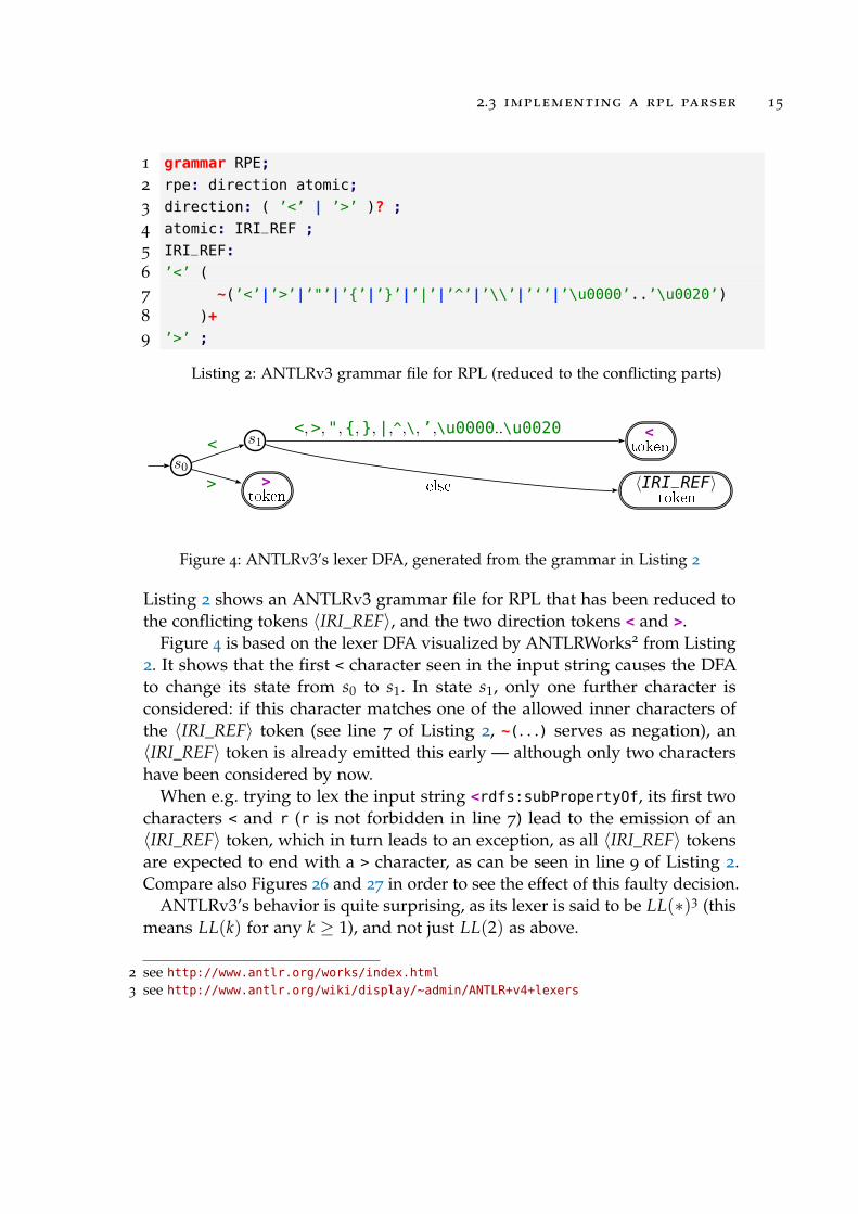
Listing 2: ANTLRv3 grammar file for RPL (reduced to the conflicting parts)
s0
s1
〈IRI_REF〉token>token <token<
>
<,>,",,,|,^,\,’,\u0000..\u0020else
1
Figure 4: ANTLRv3’s lexer DFA, generated from the grammar in Listing 2
Listing 2 shows an ANTLRv3 grammar file for RPL that has been reduced tothe conflicting tokens 〈IRI_REF〉, and the two direction tokens < and >.
Figure 4 is based on the lexer DFA visualized by ANTLRWorks2 from Listing2. It shows that the first < character seen in the input string causes the DFAto change its state from s0 to s1. In state s1, only one further character isconsidered: if this character matches one of the allowed inner characters ofthe 〈IRI_REF〉 token (see line 7 of Listing 2, ~(. . .) serves as negation), an〈IRI_REF〉 token is already emitted this early — although only two charactershave been considered by now.
When e.g. trying to lex the input string <rdfs:subPropertyOf, its first twocharacters < and r (r is not forbidden in line 7) lead to the emission of an〈IRI_REF〉 token, which in turn leads to an exception, as all 〈IRI_REF〉 tokensare expected to end with a > character, as can be seen in line 9 of Listing 2.Compare also Figures 26 and 27 in order to see the effect of this faulty decision.
ANTLRv3’s behavior is quite surprising, as its lexer is said to be LL(∗)3 (thismeans LL(k) for any k ≥ 1), and not just LL(2) as above.
2 see http://www.antlr.org/works/index.html3 see http://www.antlr.org/wiki/display/~admin/ANTLR+v4+lexers

16 preliminaries: introducing rpl
In contrast, JavaCC4 is able to cleanly keep all tokens apart. An additionaladvantage over ANTLRv3 is that it does not rely on a separate runtimecomponent — all needed classes are directly created during JavaCC parsergeneration. Figure 5 gives an overview over JavaCC’s setup for parsing RPL.The grammar file RPE.jj, which is the only input to javacc, contains both thelexer and parser rules.
JavaCC Source
RPE.jj
JavaCC Compiler
javacc
Lexical Analysis
JavaCharStream.javaToken.javaTokenMgrError.javaRPEParserConstants.javaRPEParserTokenManager.java
Syntactical Analysis
ParseException.java RPEParser.java
Figure 5: Overview of JavaCC parser generation, similar to [30]
2.4 T H E R E S O U R C E D E S C R I P T I O N F R A M E W O R K
The Resource Description Framework (RDF) is a “language for representinginformation about resources in the World Wide Web” [10]. However, RDF isnot only able to represent metadata about Web resources, but also arbitrarygraph-shaped data.
Definition 2 (RDF Triple, RDF Graph, Subject, Predicate and Object of anRDF Triple)Let U, B, and L be pairwise disjoint infinite sets of RDF URI references, RDFblank nodes, and RDF literals, respectively. An RDF triple t = (s, p, o) over U, B,and L is an element of (U ∪ B)×U × (U ∪ B ∪ L), where s is called subject, pis called predicate, and o is called object of t. An RDF graph, for the scope of thisthesis, is a finite set of RDF triples.
4 see https://javacc.dev.java.net/

2.4 the resource description framework 17
Definition 3 (Nodes, Edges, and Terms of an RDF Graph)Let G be an RDF graph. The set of nodes of G is the set of subjects and objects ofG’s RDF triples, nodes(G) := s | (s, p, o) ∈ G ∪ o | (s, p, o) ∈ G. Similarly,the set of edges of G is defined as edges(G) := p | (s, p, o) ∈ G, and the setof terms of G as terms(G) := nodes(G) ∪ edges(G).
Definition 4 (Paths in an RDF Graph)For the scope if this thesis, a path p within an RDF graph G is a sequence(n1, . . . , n2k+1), k ≥ 0 where the RDF triples (n2i−1, n2i, n2i+1) are contained inG for all 1 ≤ i ≤ k. The length of p is defined as the number of edges that pcontains, i.e. |p| := k.
An RDF graph G can also be interpreted as a directed labeled multigraphM(G) [5]. When drawing an RDF graph, each node n ∈ nodes(G) is repre-sented by its label which is drawn inside an oval (if n ∈ U ∪ B) or a rectangle (ifn ∈ L). Each edge e belonging to an RDF triple (s, e, o) is drawn as a directed,labeled arrow from the figure of s to the figure of o.
When discussing RPL, we always refer to the RDF graph presented in Figure6 unless stated otherwise. It consists of several cities that are connected to eachother via different means of transport. Additionally, Figure 6 makes use of theRDFS vocabulary [20], in order to express e.g. rdfs:subPropertyOf (which isabbreviated as rdfs:sp) and rdfs:subClassOf relationships.
RDF Serializations
RDF offers a plethora of serialization formats, of which only the currentlymost commonly used ones, RDF/XML [6] and Turtle [7] shall be mentionedhere. RDF/XML, however, is a verbose syntax and difficult to read.
Listing 3 shows a Turtle serialization of the RDF graph shown in Figure 6.The Turtle syntax is quite close to the RDF data model, as it is made up ofsingle triples that are separated by a dot character from each other. If a triple tis instead ended by a comma (semicolon), the subject and predicate (subject)of t will be reused for the subsequent triple.
Definition 5 (Size of an RDF Graph)For time complexity considerations (Chapter 3), we define the size of anRDF graph G (denoted by |G|) as the size (in characters) of its minimalrepresentation in Turtle syntax, by not making use of any namespace prefixdeclarations or abbreviations.

18 preliminaries: introducing rpl
:TGV :NExpress :Seafrance
:train :bus :ferry
:transport
:city
rdfs:sp rdfs:sp rdfs:sp
rdfs:sprdfs:sp rdfs:sp
:Paris
:Calais
:Dijon:TGV
:TGV
:Dover:Seafrance
:London
:Hastings
:NExpress:country
:France
:coastal_city
rdf:type
rdfs:subClassOf
rdfs:range
rdfs:domain
rdfs:range
rdfs:domain
:NExpress
Figure 6: RDF graph about transportation services between cities [27]
1 @prefix rdf: <http://www.w3.org/1999/02/22-rdf-syntax-ns#> .
2 @prefix rdfs: <http://www.w3.org/2000/01/rdf-schema#> .
3 @prefix : <http://example.org/> .
4
5 :Paris :TGV :Calais , :Dijon ; :country :France .
6 :Calais :Seafrance :Dover .
7 :Dover :NExpress :Hastings , :London .
8
9 :TGV rdfs:subPropertyOf :train .
10 :Seafrance rdfs:subPropertyOf :ferry .
11 :NExpress rdfs:subPropertyOf :bus .
12
13 :train rdfs:subPropertyOf :transport .
14 :ferry rdfs:subPropertyOf :transport .
15 :bus rdfs:subPropertyOf :transport .
16
17 :ferry rdfs:range :coastal_city ; rdfs:domain :coastal_city .
18 :Hastings a :coastal_city .
19
20 :transport rdfs:range :city ; rdfs:domain :city .
21 :coastal_city rdfs:subClassOf :city .
Listing 3: Turtle serialization of the RDF graph from Figure 6

2.5 excursus: regular expressions over strings 19
2.5 E X C U R S U S : R E G U L A R E X P R E S S I O N S O V E R S T R I N G S
Regular Expressions over ordinary strings are used in conjunction with
1. AtomicRPEs, which serve as edge or node label tests, and
2. ENREs (Definition 10) of the form 〈axis〉::〈regexp〉.
[13] states that regular expressions are poorly implemented in most modernprogramming languages. Concerning Java, this claim can be verified using asnippet like the one shown below.
public static void main(String[] args)
StringBuilder regexp = new StringBuilder();
StringBuilder string = new StringBuilder();
for (int i = 1; i <= 28; i++)
regexp.insert(0, "a?");
regexp.append("a");
string.append("a");
long before = System.nanoTime();
string.toString().matches(regexp.toString());
long after = System.nanoTime();
double seconds = (after - before) / 1000000000.;
System.out.println("Matching (a?)^" + i + "a^" + i + " against a^" + ←i + " took " + seconds + " s.");
...
Matching (a?)^20a^20 against a^20 took 0.180791973 s.
Matching (a?)^21a^21 against a^21 took 0.424027634 s.
Matching (a?)^22a^22 against a^22 took 0.671791247 s.
Matching (a?)^23a^23 against a^23 took 1.575839667 s.
Matching (a?)^24a^24 against a^24 took 3.72857081 s.
Matching (a?)^25a^25 against a^25 took 5.844788933 s.
Matching (a?)^26a^26 against a^26 took 13.787329395 s.
Matching (a?)^27a^27 against a^27 took 32.909819265 s.
Matching (a?)^28a^28 against a^28 took 50.436544589 s.
Java’s native regular expression implementation java.util.regex (initiated bya call of matches(String regex) on a String object in the snippet above) isbased on a backtracking approach. So, when trying to match a string againstthe pattern a?, this backtracking implementation tries first for the pattern a,and then for ε. The patterns used in the snippet are a concatenation of thesub-patterns a? (n times) and a (n times). So, for evaluating the n-th pattern,
20 preliminaries: introducing rpl
O(2n) possibilities have to be considered, and only the very last (choosing ε
for all a? sub-patterns) will lead to a match (cf. [13]).However, by constructing an ε-NFA A from a regular expression exp, the
time complexity of matching a string s to the pattern exp is O(n ·m), wheren is the length of s and m is the number of A′s states. m, however, is at mostequal to the length of exp by Thompson’s construction [32].
For this reason, we prefer the dk.brics.automaton implementation [24] overJava’s native implementation and modify it accordingly, so that no determini-sation takes place (which, in the worst case, would also require exponentialtime as it can lead to a DFA having O(2m) states, cf. [28]).

3I M P L E M E N T I N G R P L
After presenting RPL’s syntactic and semantic analysis in Section 3.1, thischapter first gives a set-based semantics of path-flavored RPL queries.
Section 3.3 presents an evaluation approach that is based on translating RPLinto an intermediate language, ENREs (Extended Nested Regular Expressions).After presenting the syntax and semantics of ENREs, we show the correctnessof the translation function and present an adapted graph labeling algorithm forENREs that is shown to have linear query and quadratic data time complexity.
Section 3.4 presents two variants of the Path-based evaluation approach.After introducing the notion of partial path matrices and the basic idea of thealgorithm (linking each subexpression e of a RPL query with a matrix thatstores all paths satisfying e), the second variant is shown to have linear queryand cubic data time complexity.
3.1 S Y N TA C T I C & S E M A N T I C A N A LY S I S
Many query languages include syntactic constructs that do not have anyeffect on the expressive power of the language, but allow users to express thesame (i.e. semantically equivalent) query in an alternative, often shorter ormore intuitive way (consider e.g. the abbreviated syntax of XPath [11]). Suchsyntactic constructs are generally known as syntactic sugar1 and are eliminatedwithin a compiler phase called syntactic analysis.
On the other hand, not all preconditions for the evaluation of a query canbe expressed on a purely syntactic level in most query languages (e.g. theexistence of all tables and columns that are referenced within an SQL query, orthe declaration of all namespace prefixes that are used within a SPARQL [29]query). These semantic checks are carried out within another compiler phasecalled semantic analysis.
1 see http://en.wikipedia.org/wiki/Syntactic_sugar
21

22 implementing rpl
An overview of RPL’s syntactic and semantic analysis is given in Figure 7.
Syntactic Analysis
Simplification Normalization
Semantic Analysis
Length verification
Direction verification
Namespace resolution
Figure 7: RPL’s syntactic and semantic analysis phases
The syntactic analysis phase of RPL is organized in two passes. During simplifi-cation, its first pass, all unnecessary parentheses are removed from a RPL query.The second pass, called normalization, then converts node- and edge-flavoredRPL queries into path-flavored ones (hence, node- and edge-flavored queriescan be considered as syntactic sugar).
Figure 8 demonstrates the syntactic analysis of the query NODES> :a (_)+.
The semantic analysis phase consists of three passes, of which each enrichesthe abstract syntax tree of a RPL query. We call a RPL query valid iff it haspassed all checks of the semantic analysis.
Its first pass, length verification, checks e.g. that the length of all possible paths(when counting each node and edge as 1) defined by a (path-flavored, due tonormalization) RPL query is an odd number, as every path must start and endwith a node. For instance, this check fails on PATH :a >:b, as it describes apath starting with a node :a that has an outgoing edge :b, but no target node.
The second pass of the semantic analysis is called direction verification. Usingthe length information that has been stored on each node of the abstract syntaxtree during the preceding pass, direction verification computes if the patha subexpression e is expected to match either starts with a node or an edge— we say that e appears at node or edge position. In this context, it is alsochecked that each DirectableRPE appearing at node position (i.e. it is expectedto match a node) is not directed by any of the direction modifiers < and >. Forinstance, PATH :a >:b <:c fails direction verification, as <:c is directed by <,but is expected to match a node.
Namespace resolution is the third pass within the semantic analysis of RPL.It resolves namespace prefixes that are defined in the underlying RDF graph,on which the RPL query is to be evaluated. Furthermore, all AtomicRPEs areenriched with a regular expression that corresponds to their string value.
Figure 9 demonstrates all passes of the semantic analysis on the RPL queryPATH :a (>_ _)+, as returned by the syntactic analysis on the original queryNODES> :a (_)+ (Figure 8).

3.1
sy
nt
ac
tic
&s
em
an
tic
an
al
ys
is
23
!"
(a) Initial query: NODES> :a (_)+
(b) After simplification: NODES> :a _+
!
"
#
#
(c) After normalization: PATH :a (>_ _)+
Figure 8: Syntactic analysis of the query NODES> :a (_)+ consists of removing unnecessary parentheses during simplifica-tion, and converting it into a path-flavored query during normalization

24
im
pl
em
en
tin
gr
pl
!"
#$%
&
!'
!'
(a) After length verification
!"
#
$%
&'!"
!"
!
( !
$)!
#
$)
(b) After direction verification
!"
#
$%
&'%((&$)('
*+!"
!"
!
, !
$-!&+
#
$-&+
(c) After namespace resolution
Figure 9: Enrichment of the abstract syntax tree in Figure 8c with lengths during length verification, positions duringdirection verification, and regular expressions for AtomicRPEs during namespace resolution

3.1 syntactic & semantic analysis 25
3.1.1 Simplification
Simplification is the first pass during the syntactic analysis of RPL queries. Itminimizes the abstract syntax tree of arbitrary RPL queries by removing allunnecessary parentheses.
Example 1
PATH ((_ >rdfs:subPropertyOf)* :transport)
gets simplified to
PATH (_ >rdfs:subPropertyOf)* :transport
Figure 10 shows the query of Example 1 before and after simplification.
!
"#$%&"
#%
!
"#$%&"
#%
Figure 10: Abstract syntax tree before (left) and after (right) simplification

26 implementing rpl
No further simplification is done beyond this. For instance,
PATH (_ >rdfs:subPropertyOf)? (_ >rdfs:subPropertyOf)* :transport
could as well be simplified to the resulting query of Example 1. The reason forthis behaviour is that the simplification pass is just considered as a preparationstep for normalization, the following pass within the syntactic analysis phase.
3.1.2 Normalization
To ease the authoring of RPL queries, node-, edge-, and path-flavored RPEs areallowed. However, for evaluation purposes, it is more convenient to deal withonly one flavor of RPEs. Hence, node- and edge-flavored RPEs are convertedinto path-flavored ones during normalization.
Example 2
EDGES >[PATH (_ >rdfs:subPropertyOf)* :transport]
is an edge-flavored RPE whose single edge is restricted by a predicate. Theequivalent path-flavored RPE is obtained by inserting a wildcard before andafter this single edge.
PATH _ >[PATH (_ >rdfs:subPropertyOf)* :transport] _
As can be seen in Example 2, the fundamental idea is to insert wildcards at theproper positions in node- and edge-flavored RPEs. More precisely, wildcardshave to be inserted at all positions of a node-flavored (edge-flavored) RPE,where an edge (a node) would be required in the corresponding path-flavoredRPE. If NODES> or NODES< is used, these wildcards also have to be directed by >
or <, respectively.In the case of node-flavored RPEs, it is crucial that the simplification pass
has already happened — otherwise, the algorithm that establishes the insertionof wildcards at the appropriate positions would not function correctly.
Example 3 demonstrates that adorned subexpressions, whose multiplicity is?, *, or +, require special treatment.
Example 3
We reuse the query of Example 2 by just adding the multiplicity +
EDGES >[PATH (_ >rdfs:subPropertyOf)* :transport]+

3.1 syntactic & semantic analysis 27
Converting this edge-flavored RPE results in two syntactically different (butsemantically equivalent) path-flavored RPEs, depending on where parenthesesare introduced.
PATH (_ >[PATH (_ >rdfs:subPropertyOf)* :transport])+ _
PATH _ (>[PATH (_ >rdfs:subPropertyOf)* :transport] _)+
The implementation of the normalization algorithm will return the first result.
One special case during normalization deserves attention: when convertingnode-flavored RPEs, the size of the query might increase exponentially undercertain conditions. If all children of a concatenated expression are adornedsubexpressions with multiplicity +, then one of these adorned subexpressionsmust be unrolled as shown in the UML object diagram in Figure 11. As isthe case with ordinary regular expressions, unrolling has no effect on thesemantics of the query.
multiplicity = PLUS=⇒
unroll
multiplicity = ONE multiplicity = STAR
Figure 11: Unrolling +-adorned expressions
The exponential increase of the query size is reached when a query nestsseveral +-adorned expressions into one another, like Example 4 demonstrates.
However, there is no way to bypass unrolling in this case, as both evaluationalgorithms (Sections 3.3 and 3.4) are designed to only work on path-flavoredRPEs.
Example 4
In order to illustrate this special case, consider the following query
NODES> (:a [NODES> :b+])+
Unrolling transforms it to
NODES> (:a [NODES> :b :b*]) (:a [NODES> :b :b*])*
The final path-flavored RPE is
PATH (:a >_ [PATH :b (>_ :b)*]) (>_ (:a >_ [PATH :b (>_ :b)*]))*

28 implementing rpl
3.1.3 Length Verification
Length verification is the first pass of the semantic analysis phase. It calculatesthe length of all possible paths that are defined by a RPL query and itssubexpressions. However, for this calculation, it is not necessary to count thetotal number of nodes and edges that have to be traversed — it is sufficient toknow if a path has odd or even length.
After these lengths have been calculated and stored in the abstract syntaxtree (Figures 2 and 3) , several checks are carried out. For instance, as path-flavored queries always start and end with a node, the length of its possiblepaths has to be odd in any case. Let us study the example query PATH :a >:b.It defines a path starting at a node :a that has an outgoing edge :b, but notarget node. Although we are already sure that this query is incorrect, we tryto intuitively determine its length. :a matches a single node, so its length isodd, and >:b matches a single edge, so its length is odd as well. The length ofthe concatenation :a >:b is obtained by “adding” the length of its children.Concatenating two paths of odd length however yields a path of even length(as is the case when adding two odd numbers), and this will cause lengthverification to fail on PATH :a >:b.
The following Definitions 6 and 7 formalize this intuition.
Definition 6 (Lengths, Addition of Lengths)Let lengths := EVEN, ODD be the set of lengths. The addition of two lengthslength1, length2 ∈ lengths is defined as
length1 + length2 :=
EVEN if length1 = length2
ODD else
Definition 7 (Length of RPEs)Let lengths := EVEN, ODD be the set of lengths. The length of an RPE, length :RPE 7→ lengths ∪ ⊥ is inductively defined as follows. The notation usedwithin the following boxes is explained in Section 2.2.2.
Let atomic be an AtomicRPE. length(atomic) := ODD
Let predicate be a PredicateRPE.
length(predicate) :=
⊥ if length(predicate.getFlavored()) = ⊥ODD else

3.1 syntactic & semantic analysis 29
Let p be a PredicatesRPE and children := p.getPredicates().
length(p) :=
⊥ if ∃child ∈ children : length(child) = ⊥ODD else
Let directed be a DirectedRPE.length(directed) := length(directed.getDirectable())
Let d be a DisjunctiveRPE and children := d.getConcatenateds().
length(d) :=
len if ∀child ∈ children : length(child) = len
⊥ else
Let a be an AdornedRPE and adornable := a.getAdornable().
length(a) :=
EVEN if length(adornable) = EVEN
ODD if length(adornable) = ODD ∧a.getMultiplicity() = ONE
⊥ else
Let c be a ConcatenatedRPE and children := c.getAdorneds().
length(c) :=
∑child∈children length(child)
if ∀child ∈ children : length(child) 6= ⊥⊥ else
Let f be a FlavoredRPE.
length( f ) :=
ODD if length( f .getConcatenated()) = ODD
⊥ else
There are three cases within Definition 6, where ⊥ is returned as the length ofan RPE (Figure 3), while all of its children have a length different from ⊥.
1. All children of a DisjunctiveRPE need to have either ODD or EVEN length.Hence, (:a :b :c | :d) is allowed, while (:a :b | :c) is not (theConcatenatedRPEs :a :b and :c have EVEN and ODD length, respectively).
2. If the length of an AdornableRPE is ODD, then the multiplicity of its parentAdornedRPE must be ONE. In all other cases, the length of this AdornedRPE

30 implementing rpl
is undefined. For instance, :a+ would be of ODD length, if the multiplicity+ is expanded only once (resulting in :a), but it would be of EVEN length,if + is expanded twice (resulting in :a :a).
3. A ConcatenatedRPE, which is child of a FlavoredRPE, must be of ODD
length, as every path is of ODD length. E.g., PATH :a >:b describes a pathstarting with a node :a that has an outgoing edge :b, but no target node.(PATH :a >:b _ would be a valid expression)
From an implementation point of view, an RPELengthException is thrownif the length function returns ⊥. This yields an error message as shown inExample 5.
Example 5
Length verification of PATH (:a :b | :c) is unsuccessful (according to thefirst of the above three cases) and yields the following error message.
Expression ":c" has odd length:
PATH (:a :b | :c)
^^
3.1.4 Direction Verification
In the previous pass of the semantic analysis, we have calculated the lengthof a RPL query and all of its subexpressions. When further processing theselengths, we can determine if a subexpression e has to start with a node oran edge label test by calculating the length of its preceding subexpressions.This enables us to check if e is allowed to be directed by < or >, as directionmodifiers should only be used on edge label tests2.
Example 6
The RPL query PATH :a >:b <:c consists of three atomic expressions, where:a is a node test, >:b is an edge test and <:c in turn is a node test that is invalid,as it is directed by <. Hence, the direction verification of PATH :a >:b <:c failswith the following error message.
2 It is arguable if really an error should be thrown if the user tries to apply a direction modifieron node label tests, as the RPL query could still be evaluated by just ignoring this modifier.However, we believe that giving the user a chance to reconsider his query by rejecting it is thebest option.

3.1 syntactic & semantic analysis 31
Expression ":c" appears at NODE position and cannot be directed:
PATH :a >:b <:c
^^
We say that a subexpression e appears at NODE and EDGE position, if the pathdefined by e has to start with a node and edge label test, respectively. Formally,a position can be defined as an element of the set of positions := EDGE, NODE,and these positions can be efficiently computed via a single top-down traversalas follows.
1. The position of a FlavoredRPE is always NODE.
2. If adorned1, . . . , adornedn are the children of a ConcatenatedRPE c, theirposition is defined as
position(adornedi) := position(c) +i−1
∑j=0
length(adornedj)
(1 ≤ i ≤ n, and ∑0j=0 length(adornedj) := EVEN)
3. In all remaining cases, the position of an RPE is inherited from its parent.
In the second case, we add a length to a position, which is defined as follows.The idea is that a position stays unchanged when adding an EVEN length, andchanges (from EDGE to NODE or from NODE to EDGE) when adding an ODD length.
Definition 8 (Addition of lengths to positions)The addition of a position pos ∈ EDGE, NODE and a length len ∈ EVEN, ODDis defined as
pos + len :=
pos if len = EVEN
EDGE if len = ODD∧ pos = NODE
NODE if len = ODD∧ pos = EDGE
Once the position of all elements in the abstract syntax tree has been com-puted, the remaining check is to verify that no DirectableRPE (which canbe an AtomicRPE or a PredicatesRPE) appears at NODE position and is di-rected by < or > (i.e. the direction of its parent DirectedRPE must be equal toDIRECTION.UNDIRECTED).
If this check fails, an RPEDirectionException like shown in Example 6 isthrown.

32 implementing rpl
3.1.5 Namespace Resolution
So far, the order of the presented passes within the syntactic and semanticanalysis was determined by the way they rely on each other. The namespaceresolution of AtomicRPEs in contrast can be done at any stage during thisanalysis.
Each namespace prefix that is used in a RPL query has to be declared within theRDF data against it is to be evaluated. Otherwise, an RPENamespaceException
will be thrown. If using RPL as embedded language (Chapter 4), the namespaceprefix declarations from the enclosing host query will be taken into accountinstead.
Example 7
Namespace resolution fails with an error message, if any undeclared names-pace prefix is used. In the expression below, the prefix rdfs: has not beendeclared in the corresponding RDF data.
Namespace prefix "rdfs:" cannot be resolved:
PATH _ >rdfs:range _
^^^^^^^^^^
Apart from namespace resolution, a second task is done during this pass: thegeneration of (ordinary) regular expressions from all kinds (LITERAL, WILDCARD,IRI, . . ., see Figure 2) of AtomicRPEs.
This is possible, since regular expressions are powerful enough to embedall those kinds. Furthermore, matching strings against a regular expressioncreated from e.g. a 〈STRING_LITERAL1〉 token (Definition 1) has the samecomplexity as comparing these two strings character by character, as theresulting automaton is already deterministic.
Example 8
The string literal "Harald" (interpreted as a regular expression) translates tothe following automaton.
” H a r a l d ”

3.2 semantics of rpl 33
3.2 S E M A N T I C S O F R P L
In this section, we define the semantics of RPL. A compositional semanticsof RPL has already been given in [9]. We have chosen not to adapt thesedefinitions to the current version of RPL, as their correctness has not beenshown. Instead, we give a purely set-based semantics of RPL.
Definition 9 (Semantics of RPL)The semantics of a path-flavored RPE f over an RDF graph G (Definition 2)is given as [[[ f ]]]G, where [[[·]]]G is inductively defined as follows. The notationused within the following boxes is explained in Section 2.2.2.
Let a be an AtomicRPE, pos := a.getPosition(), rx := a.getRegExp(), and dir aDIRECTION.Case pos = NODE
[[[a]]]G := (n, n) | ∃n ∈ nodes(G) ∧ n ∈ L(rx)Case pos = EDGE
[[[a]]]dirG :=
(s, o) | ∃p : (s, p, o) ∈ G ∧ p ∈ L(rx) if dir = FORWARD
(o, s) | ∃p : (s, p, o) ∈ G ∧ p ∈ L(rx) if dir = BACKWARD
[[[a]]]FORWARDG ∪ [[[a]]]BACKWARDG if dir = UNDIRECTED
Let p be a PredicateRPE, f := p.getFlavored(), pos := p.getPosition(), ands := p.getSign().Case pos = NODE
[[[p]]]G :=
(n, n) | n ∈ nodes(G) ∧ ∃q : (n, q) ∈ [[[ f ]]]G if s=POSITIVE
(n, n) | n ∈ nodes(G) ∧ @q : (n, q) ∈ [[[ f ]]]G if s=NEGATIVECase pos = EDGE
[[[p]]]G :=
(e, e) | e ∈ edges(G) ∧ ∃q : (e, q) ∈ [[[ f ]]]G if s = POSITIVE
(e, e) | e ∈ edges(G) ∧ @q : (e, q) ∈ [[[ f ]]]G if s = NEGATIVE

34 implementing rpl
Let p be a PredicatesRPE, p1, p2, . . . , pn (n ≥ 1) its children, pos :=p.getPosition(), and dir a DIRECTION.Case pos = NODE
[[[p]]]G := (n, n) | n ∈ nodes(G) ∧ (n, n) ∈ [[[p1]]]G . . . [[[pn]]]GCase pos = EDGE
[[[p]]]dirG :=(s, o) | ∃(s, e, o) ∈ G ∧ (e, e) ∈ [[[p1]]]G . . . [[[pn]]]G if dir = FORWARD
(o, s) | (s, o) ∈ [[[p]]]FORWARDG if dir = BACKWARD
[[[p]]]FORWARDG ∪ [[[p]]]BACKWARDG if dir = UNDIRECTED
Let d be a DirectedRPE and direction := d.getDirection().[[[d]]]G := [[[d.getDirectable()]]]direction
G
Let d be a DisjunctiveRPE and c1, c2, . . . , cn(n ≥ 1) its children.[[[d]]]G := [[[c1]]]G ∪ [[[c2]]]G ∪ . . . ∪ [[[cn]]]G
Let a be an AdornedRPE, ad := a.getAdornable(), and mult :=a.getMultiplicity().
[[[a]]]G :=
[[[ad]]]G if mult = ONE
(v, v) | v ∈ terms(G) ∪ [[[ad]]]G if mult = OPT
(v, v) | v ∈ terms(G) ∪ [[[ad + ]]]G if mult = STAR
[[[ad]]]G ∪ [[[ad]]]G [[[ad]]]G ∪ . . . if mult = PLUS
Let c be a ConcatenatedRPE and a1, a2, . . . , an(n ≥ 1) its children.[[[c]]]G := [[[a1]]]G [[[a2]]]G . . . [[[an]]]G
Let f lavored be a FlavoredRPE.[[[ f lavored]]]G := [[[ f lavored.getConcatenated()]]]G
with X Y := (x, z) | ∃y : (x, y) ∈ X ∧ (y, z) ∈ Y (this operator is used forAdornedRPEs, ConcatenatedRPEs and PredicatesRPEs).
3.3 E N R E - B A S E D E VA L U AT I O N
NREs (Nested Regular Expressions) have been presented in [27] as a means todescribe and query regular paths in RDF graphs. The proposed graph labeling

3.3 enre-based evaluation 35
algorithm for the evaluation of NREs has been shown to have polynomialcombined, and linear data and query time complexity, when considering thecomplexity of the associated decision problem.
In this thesis, we present ENREs, an extended version of NREs designed toaddress the characteristics of RPL: regular expressions (over ordinary strings)as node and edge label tests, as well as the negation of predicates (which arecalled nested expressions in the case of ENREs).
The syntax and semantics of ENREs is given in Section 3.3.1.In Section 3.3.2, we show that RPL queries can be translated into ENREs in
linear time, and that this translation is correct in regard to the semantics of RPL(Section 3.2) and ENREs. It is also shown that the semantics of ENREs, whichhave been constructed by translating a RPL query, is a subset of nodes(G)×nodes(G), with G being an RDF graph (Definitions 2 and 3).
In Section 3.3.3, we present an adapted version of the graph labeling al-gorithm for NREs, which relies on constructing product automata from theunderlying RDF graph for each nested expression of an ENRE.
Finally, we formally prove that the time complexity (i.e. the complexitywhich is actually needed when constructing the result set of a query, see [1]— rather than the complexity of just deciding whether a certain pair of RDFterms is in the result set or not) is quadratic in the size of the data and linearin the size of the query, as is the case for NREs [27]. Hence, evaluating RPL byusing ENREs as an intermediate language is as efficient as evaluating NREs(which are less expressive).
3.3.1 Syntax and Semantics of ENREs
Definition 10 (Abstract Syntax of ENREs)The abstract syntax of ENREs is defined by the following grammar.
〈enre〉 ::= 〈enre〉 ‘/’ 〈enre〉 |〈enre〉 ‘|’ 〈enre〉 |〈enre〉 (‘?’ | ‘*’ | ‘+’) |〈axis〉 |〈axis〉 ‘::’ 〈regexp〉 |〈axis〉 ‘::’ 〈nested〉
〈nested〉 ::= ‘!’? ‘[’ 〈enre〉 ‘]’
〈axis〉 ::= ‘next’ | ‘next−1’ | ‘next_or_next−1’ |‘self_node’ | ‘self_edge’

36 implementing rpl
Definition 10 gives just an abstract syntax, hence it is not targeted at parsingENREs. The optionality operator and the Kleene star and plus operators (?, *,and +) bind more strongly than the concatenation operator /, which in turnbinds more strongly than the alternative operator |. Parentheses will be used,whenever these precedence rules need to be overridden.
Definition 10 both extends and limits the definition given in [27].
• The navigation axes (see the 〈axis〉 rule) self, edge, edge−1, node, andnode−1 are omitted, as they are not needed when evaluating RPL. On theother hand, new axes are introduced to express the peculiarities of RPL:self_node and self_edge act like self, but filter for nodes and edges,respectively. The new axis next_or_next−1 is used for undirected edgenavigation and is satisfied iff next or next−1 holds.
• Like RPEs, ENREs support the negation (indicated by !) of nested expres-sions (see the 〈nested〉 rule), which are called predicates in RPL (bothnested expressions and predicates are enclosed by brackets).
• Via the 〈regexp〉 rule, ENREs allow to use regular expressions (overordinary strings) for node and edge label tests, while NREs only allowedfor IRIs.
Example 9
Let us consider the following example query, to be evaluated on an RDF graphG (Definition 2).
self_node:::Paris/next::![self_edge:::TGV]
It expresses a path that starts at a node of G (because of the self_node axis)labeled with :Paris, followed by a next move. The next axis moves from thesubject to the object of an RDF triple (Definition 2), and is able to expressrestrictions on its predicate (see also Figure 28). In our case, this restrictionconsists of the nested expression ![self_edge:::TGV], which matches everyedge of G not (indicated by !) labeled with :TGV.
Evaluating this ENRE on the RDF graph from Figure 6 will lead to the resultset (:Paris, :France), as the node :Paris has an outgoing edge labeledwith :country that reaches the node :France. The other two outgoing edgesof :Paris, labeled with :TGV, are not followed as they do not satisfy the nestedexpression ![self_edge:::TGV].
In the preceding example, we have already (informally) come across thesemantics of ENREs, which is now formally given in Definition 11.

3.3 enre-based evaluation 37
Definition 11 (Semantics of ENREs)The semantics of an ENRE exp over an RDF graph G is given as JexpKG, whereJ·KG is inductively defined as follows. In general, the result of J·KG is a subsetof terms(G)× terms(G) (Definition 2).
Jself_nodeKG := (n, n) | n ∈ nodes(G)Jself_node::αKG := (n, n) | n ∈ nodes(G) ∧ condG
α (n)
Jself_edgeKG := (p, p) | p ∈ edges(G)Jself_edge::αKG := (p, p) | p ∈ edges(G) ∧ condG
α (p)
JnextKG := (s, o) | ∃p : (s, p, o) ∈ GJnext::αKG := (s, o) | ∃p : (s, p, o) ∈ G ∧ condG
α (p)
Jnext−1KG := (o, s) | (s, o) ∈ JnextKGJnext−1::αKG := (o, s) | (s, o) ∈ Jnext::αKG
Jnext_or_next−1KG := JnextKG ∪ Jnext−1KG
Jnext_or_next−1::αKG := Jnext::αKG ∪ Jnext−1::αKG
where condGα (x) :=
x ∈ L(regexp) if α = regexp
∃q ∈ terms(G) : (x, q) ∈ JexpKG if α = [exp]
@q ∈ terms(G) : (x, q) ∈ JexpKG if α = ![exp]
Jexp1|exp2KG := Jexp1KG ∪ Jexp2KG
Jexp1/exp2KG := Jexp1KG Jexp2KG, whereX Y := (x, z) | ∃y : (x, y) ∈ X ∧ (y, z) ∈ Y
Jexp ?KG := Jself_nodeKG ∪ Jself_edgeKG ∪ JexpKG
Jexp*KG := Jself_nodeKG ∪ Jself_edgeKG ∪ Jexp+ KG
Jexp+ KG := JexpKG ∪ Jexp/expKG ∪ Jexp/exp/expKG ∪ . . .

38 implementing rpl
3.3.2 Translating RPL into ENREs
After having defined the syntax and semantics of ENREs, the missing linkbetween RPL and ENREs is established: a translation function trans that mapsRPEs to ENREs. This translation should be easy to compute (i.e. in linear timeof the length of its source query), and, of course, correct in the sense thatthe semantics of a RPL query q (Definition 9) coincides with the semantics oftrans(q) (Definition 11).
The following Example might give an idea of how such a translation can beconstructed.
Example 10
Consider the following RPL query q
PATH _ >p _ with p :=[PATH (_ >rdfs:subPropertyOf)* :transport]
During semantic analysis (Section 3.1), the AtomicRPEs rdfs:subPropertyOf
and :transport got enriched with their corresponding regular expressionsr1 := http://www.w3.org/2000/01/rdf-schema#subPropertyOf and r2 := http:
//example.org/transport, respectively.The translation function (Definition 13) will return the following ENRE e
self_node/next::[α]/self_node withα := self_edge::[β]
β := (self_node/next::r1)*/self_node::r2
The ENRE β corresponds to PATH (_ >rdfs:subPropertyOf)* :transport,the flavored child of q’s predicate p. p appears at EDGE position within q, so β
is used as a nested expression to restrict the self_edge move, and thus we getto the ENRE α.
q itself just consists of a wildcard (at NODE position) that has an outgoingedge (at EDGE position) satisfying p to another wildcard (again at NODE position).Each of the wildcards can be translated via a self_node move, and jumpingfrom the first to second wildcard is done via a next move satisfying α (see alsoFigure 28).
Having seen this example translation, we continue by giving a formal definitionof the translation function trans (Definition 13), preceded by its helper functiongetAxis (Definition 12).

3.3 enre-based evaluation 39
Definition 12 (Helper Function getAxis)The helper function getAxis, which is used in the following translation func-tion, maps a position (Section 3.1.4) and a DIRECTION (FORWARD, BACKWARD, orUNDIRECTED) to an ENRE navigation axis as follows.
getAxis(pos, dir) :=
self_node if pos = NODE
next if pos = EDGE∧ dir = FORWARD
next−1 if pos = EDGE∧ dir = BACKWARD
next_or_next−1 if pos = EDGE∧ dir = UNDIRECTED
Within trans, this helper function is used in the case of DirectableRPEs (whichcan be AtomicRPEs and PredicatesRPEs, compare Figure 2) in order to deter-mine the appropriate ENRE navigation axis.
Definition 13 (Translation Function trans)With the help of Definition 12, we inductively define a translation functiontrans that maps an RPE to an ENRE. The notation used within the followingboxes is explained in Section 2.2.2.Let a be an AtomicRPE and dir a DIRECTION.transdir(a) := getAxis(a.getPosition(), dir)::a.getRegExp()
Let p be a PredicateRPE, pos := p.getPosition(), f := p.getFlavored(), ands := p.getSign().
trans(p) :=
axis::[trans( f )] if s = SIGN.POSITIVE
axis::![trans( f )] else
where axis :=
self_node if pos = NODE
self_edge if pos = EDGE
Let p be a PredicatesRPE, p1, p2, . . . , pn(n ≥ 1) its children, pos :=p.getPosition(), and dir a DIRECTION.transdir(p) := getAxis(pos, dir)::[trans(p1)/trans(p2)/. . ./trans(pn)]
Let d be a DirectedRPE and direction := d.getDirection().trans(d) := transdirection(d.getDirectable())
Let d be a DisjunctiveRPE and c1, c2, . . . , cn(n ≥ 1) its children.trans(d) := trans(c1)|trans(c2)|. . .|trans(cn)

40 implementing rpl
Let a be an AdornedRPE, adornable := a.getAdornable(), and mult :=a.getMultiplicity().
trans(a) :=
trans(adornable) if mult = MULTIPLICITY.ONE
trans(adornable)? if mult = MULTIPLICITY.OPT
trans(adornable)* if mult = MULTIPLICITY.STAR
trans(adornable)+ if mult = MULTIPLICITY.PLUS
Let c be a ConcatenatedRPE and a1, a2, . . . , an(n ≥ 1) its children.trans(c) := trans(a1)/trans(a2)/. . ./trans(an)
Let f lavored be a FlavoredRPE.trans( f lavored) := trans( f lavored.getConcatenated())
The remaining part of this section shows that the semantics of a valid RPLquery over an RDF graph G always evaluates to a subset of nodes(G) ×nodes(G) (Theorem 1 and Corollary 1), and the correctness of the transla-tion function trans (Theorem 2).
The following Lemmas 1 and 2 serve as preparation for Theorem 1.
Lemma 1
Let d be a DirectableRPE that appears at NODE position, i.e. d.getPosition() =NODE. Then Jtrans(d)KG ⊆ nodes(G) × nodes(G), with G an RDF graph andtrans as in Definition 13.
Proof. d can either be an AtomicRPE or a PredicatesRPE (Figure 2).
Case d is an AtomicRPE
Then, by Definitions 12 and 13, trans(d) = self_node::d.getRegExp(). ByDefinition 11, Jself_node::d.getRegExp()KG ⊆ (n, n) | n ∈ nodes(G) ⊆nodes(G)× nodes(G).
Case d is a PredicatesRPE
In this case, trans(d) = self_node::[trans(p1)/trans(p2)/. . ./trans(pn)], wherep1, . . . , pn are the children of d (by Definitions 12 and 13). Then, by Definition11, Jtrans(d)KG ⊆ (n, n) | n ∈ nodes(G) ⊆ nodes(G)× nodes(G).
Lemma 2
Let c be a ConcatenatedRPE and a1, . . . , an (n ≥ 1) be the adorned childrenof c. If there exists an i ∈ 1, . . . , n such that the ENRE-based semantics of

3.3 enre-based evaluation 41
ai contains just pairs of nodes of an RDF graph G, the same applies to c, i.e.Jtrans(ai)KG ⊆ nodes(G)× nodes(G)⇒ Jtrans(c)KG ⊆ nodes(G)× nodes(G).
Proof. If n = 1, we are finished as trans(c) = trans(a1) by Definition 13, andthus Jtrans(c)KG = Jtrans(a1)KG ⊆ nodes(G)× nodes(G) by assumption.
Let n > 1. Applying the rules from Definitions 11 and 13, we get Jtrans(c)KG =Jtrans(a1)KG . . . Jtrans(ai)KG . . . Jtrans(an)KG, where the concatenation op-erator is defined as X Y := (x, z) | ∃y : (x, y) ∈ X ∧ (y, z) ∈ Y. Asfor all j ∈ 1, . . . , n, Jtrans(aj)KG never contains a pair (e, n) or (n, e) withe ∈ edges(G) \ nodes(G) and n ∈ nodes(G) \ edges(G) (there is no case in Defi-nition 11, where such pairs are returned), only connects nodes with nodesand edges and edges. As Jtrans(ai)KG is a subset of nodes(G) × nodes(G),also Jtrans(ai−1)KG Jtrans(ai)KG (if i > 1) and Jtrans(ai)KG Jtrans(ai+1)KG(if i < n) are subsets of nodes(G) × nodes(G). By induction, it follows thatJtrans(c)KG ⊆ nodes(G)× nodes(G).
Theorem 1
Let f be a valid FlavoredRPE, i.e. f has passed all checks of the semanticanalysis phase (Section 3.1). The ENRE-semantics of f returns pairs of nodesof an RDF graph G, i.e. Jtrans( f )KG ⊆ nodes(G)× nodes(G).
Proof. By assumption, f has ODD length (the length verification pass wouldhave failed otherwise, see Section 3.1.3). Let c be the concatenated child of f .As the length of f is defined as the length of its child c, c has also ODD length(Definition 7).
Since the length of c is ODD, it must have at least one adorned child, whoselength is also ODD (by Definition 7). Furthermore, its multiplicity is ONE, as eachother multiplicity would imply EVEN length (also by Definition 7).
Case There exists exactly one such adorned child aa appears at NODE position, since all other adorned children have EVEN lengthin this case. However, adding EVEN arbitrarily many times to the position NODE
(which is the initial position of f and c) has no effect at all (Section 3.1.4).
Case There exist several such adorned childrenLet a denote the first of these adorned children. In this case, all adornedchildren of c which appear left of a have EVEN length. With the same argumentas above, a appears at NODE position.
This AdornedRPE a has an adornable child, which is a directed or disjunctivesubexpression.

42 implementing rpl
Case a has a directed childThis directed child is the parent of a directable subexpression d. By Lemma 1,Jtrans(d)KG ⊆ nodes(G)× nodes(G).
Case a has a disjunctive childThis disjunctive child d consists of at least two concatenated children (this isdue to the simplification pass, see Section 3.1.1) – each of them has ODD length,and appears at NODE position. So, the argument given above for the outermostconcatenated expression c can be repeated for each concatenated child of d.Hence, by induction, Lemma 2 can be applied on all children child1, . . . , childnof d yielding Jtrans(childi)KG ⊆ nodes(G)× nodes(G) for all i ∈ 1, . . . , n. ByDefinitions 13 and 11, it follows that Jtrans(d)KG =
⋃ni=1Jtrans(childi)KG ⊆
nodes(G)× nodes(G).
As a’s multiplicity is ONE, Jtrans(a)KG = Jtrans(d)KG by Definition 13. As a is achild of c, we can now apply Lemma 2 on c, which (together with Definition13) yields Jtrans( f )KG = Jtrans(c)KG ⊆ nodes(G)× nodes(G), which is whatwe wanted to show.
Theorem 2
Let q be a valid RPE and G an arbitrary RDF graph. Its semantics [[[q]]]G isequal to translating q into an ENRE and then applying the ENRE-semanticsJtrans(q)KG, i.e. [[[q]]]G = Jtrans(q)KG.
Proof. By structural induction, see Section A.1.
Corollary 1
Let f be a valid FlavoredRPE. The semantics of f over an RDF graph G, [[[ f ]]]Gis a subset of nodes(G)× nodes(G).
Proof. This is a direct consequence of Theorems 1 and 2.
3.3.3 Graph Labeling Algorithm
The graph labeling algorithm presented in this section is based on the graphlabeling algorithm for NREs [27], but has been adapted for ENREs. Moreprecisely, it supports regular expressions over strings and the negation ofnested expressions, as well as the additional navigation axes available forENREs (Section 3.3.1).

3.3 enre-based evaluation 43
The basic idea of the algorithm is that both an RDF graph G and an ENRE expcan be interpreted as NFAs (Definitions 14, 15, and 17) and combined togetherinto a product automaton (Definition 18). Such a product automaton is not onlybuilt from G and exp, but from G and all nested expressions of exp in a bottom-up manner (i.e. the product automaton belonging to the innermost nestedexpression of exp is constructed first). Each node or edge of G gets labeledwith all nested expressions that it satisfies (hence the name “graph labelingalgorithm”), and these labels are taken into account for constructing all outerproduct automata. Each constructed product automaton P is decomposed intoits strongly connected components by Tarjan’s algorithm (Section A.2), in orderto efficiently compute all initial states from which final states are reached in P .
Finally, all these steps are combined into a LABEL (Listing 4) and an EVAL
(Listing 5) method, which together implement the Graph Labeling Algorithm.
Definition 14 (Nondeterministic Finite Automaton)An NFA (Nondeterministic Finite Automaton) A is a 5-tuple (S, Σ, δ, I, F)consisting of a finite set of states S, a finite set of input symbols (i.e. thealphabet) Σ with S ∩ Σ = ∅, a transition function δ : S × Σ → 2S, a set ofinitial states I ⊆ S, and a set of final states F ⊆ S. By 2S, we denote thepower set of S. An ε-NFA is an NFA that also allows for ε transitions, i.e.δ : S× (Σ ∪ ε)→ 2S.
An alternative definition of NFAs, which only allows for a single initial state q0,is given in [21]. However, Definition 14 (also given in [28]) is more convenientin our case, as Definition 15 will show.
As the RDF graph from Figure 6 is too large to illustrate the followingconstructions, we hence rely on the RDF graph from the following Figure 12
for that purpose.
:a :b :c:e1 :d:e2 :e3
:e4
Figure 12: A simple RDF graph
Definition 15 (Interpreting an RDF Graph as NFA)Let G be an RDF graph. The corresponding NFA G is defined as G :=(terms(G), E, δG , terms(G), terms(G)). E is the set of input symbols and con-tains ENREs of the form 〈axis〉::〈regexp〉, where 〈axis〉 ∈ self_node, self_edge,

44 implementing rpl
next, next−1 and 〈regexp〉 is an arbitrary element of terms(G). The transitionfunction δG is defined as follows.
δG(v, e) :=
v if v ∈ nodes(G) ∧ e = self_node::v
v if v ∈ edges(G) ∧ e = self_edge::v
o | (v, p, o) ∈ G if e = next::p
s | (s, p, v) ∈ G if e = next−1::p
For later complexity considerations, we define the size of G as the sum of thestring lengths of its transition labels, i.e. |G| := ∑
(v,l,v′)∈δG
|l|.
Example 11
Figure 13 shows the NFA G corresponding to the RDF graph presented inFigure 12. Each state of G is both an initial and final state.
:e1 :e2 :e3 :e4
:a :b :c :d
self_edge:::e1 self_edge:::e2 self_edge:::e3 self_edge:::e4
self_node:::a self_node:::b self_node:::c self_node:::d
next−1:::e1
next:::e1
next−1:::e2
next:::e2
next−1:::e3
next:::e3
next:::e4
next−1:::e4
1
Figure 13: Interpreting the RDF graph from Figure 12 as an NFA
With Definition 15, we already have the first ingredient for the constructionof the product automaton (Definition 18). The second ingredient is an ENREthat is converted into another NFA by Thompson’s construction [32]. Priorto presenting this construction in Definition 17, we have to recall that anENRE (Extended Nested Regular Expression) exp is indeed a regular expression,namely over the alphabet D0(exp), as given in the following Definition 16.

3.3 enre-based evaluation 45
Definition 16 (Depth-0 Terms of an ENRE)The set of depth-0 terms of an ENRE exp is inductively defined as follows.
D0(exp) :=
D0(e1) ∪D0(e2) if exp = e1/e2, or exp = e1|e2
D0(e) if exp = e?, exp = e*, or exp = e+
exp otherwise
It is important to see that D0 does not decompose the nested expressions ofexp (for these, the third case applies).
Definition 17 (Interpreting an ENRE as NFA)Let exp be an ENRE. exp can be interpreted as a regular expression overthe alphabet D0(exp), which in turn can be translated into an ε-NFA Aexp =(Q, D0(exp), δA, I, F).
This translation known as Thompson’s construction has already been pre-sented in [32] and [13] for regular expressions over an arbitrary alphabet. Itdiffers from the well-known illustration in [21], as no temporary final states (i.e.states which are not final in the end result) are created during the translationprocess, which makes it straightforward to implement.
Instead of constructing a complete ε-NFA in each single translation step,we just construct partial ε-NFAs for each subexpression. Partial ε-NFAs haveno final states, but dangling arrows that are pointing at nothing. After theoutermost partial ε-NFA has been constructed, each of its dangling arrows willbe connected to a final state, which finally turns it into an ε-NFA.
Let a be an ENRE of theform 〈axis〉, 〈axis〉::〈regexp〉, or〈axis〉::〈nested〉. The partial ε-NFAfor a is
a
1
In the following boxes, Ae denotes the (recursively constructed) partial NFAthat belongs to a subexpression e. The inner state drawn left to the label Ae isAe’s initial state. The inner state drawn right to the label Ae is a fictitious state,just as if all of Ae’s dangling arrows originated from this single state.

46 implementing rpl
Let e1 and e2 be two ENREs. Theconcatenation e1/e2 is translatedinto the partial ε-NFA
Ae1 Ae2
1
Let e1 and e2 be two ENREs. Thealternative e1|e2 is translated intothe partial ε-NFA
Ae2
Ae1ε
ε
1
Let e be an ENRE. The optionalitye? is translated into the partial ε-NFA
Aeε
ε
1
Let e be an ENRE. The Kleene starexpression e* is translated into thepartial ε-NFA
Aeε
ε
1
Let e be an ENRE. The Kleene plusexpression e+ is translated into thepartial ε-NFA Ae ε
ε
1

3.3 enre-based evaluation 47
For later complexity considerations (Section 3.3.4), we define the size of Aexpas the sum of the sizes of all its transition labels, i.e.
|Aexp| := ∑(q,l,q′)∈δA
|l|
where |l| denotes the string length of the transition label l, except in thefollowing two cases. (1) The length of an ε-transition is defined as one, i.e.|ε| := 1, and (2) the length of transitions labeled with nested expressions exp′
of the form axis::nested only includes the length of its navigation axis axis, i.e.|exp′| := |axis|. The latter exception is motivated by the construction of Aexp,as nested expressions are treated as single symbols and not further split up.This coincides with the definition of D0 (Definition 16), which also does notdecompose nested expressions.
Example 12
Let us consider the ENRE self_node:::a/(next/self_node)+. We constructits corresponding NFA Aexp according to Definition 17, in a bottom-up manner.
next translates to the partial NFA (1) next self_node self_node:::a
1
self_node translates to the partial NFA (2)next self_node self_node:::a
1
next/self_node translates to thepartial NFA (3), combining its chil-dren (1) and (2)
next self_node
1
(next/self_node)+ trans-lates to the partial NFA (4),using its child (3) next self_node ε
ε
1
self_node:::a translates to the partial NFA (5)next self_node self_node:::a
1
self_node:::a/(next/self_node)+ translates to the partial NFA (6) by com-bining its children (4) and (5)
self_node:::a next self_node ε
ε
1

48 implementing rpl
Finally, the partial NFA (6) is converted into the ε-NFA below. The states havebeen numbered, as this automaton will be reused in Example 13.
0 41 2 3self_node:::a next self_node ε
ε
1
We have seen how to interpret both an RDF graph and an ENRE as NFAs(Definitions 15 and 17). The resulting NFAs G and Aexp are now combinedinto a product automaton. This product automaton P should only perform atransition, if both underlying transitions of G and Aexp “match”.
Definition 18 (Product Automaton)Let G := (terms(G), E, δG , terms(G), terms(G)) be the NFA that corresponds toan RDF graph G (in the sense of Definition 15), andAexp = (Q, D0(exp), δA, I, F)the ε-NFA that corresponds to an ENRE exp (in the sense of Definition 17).The product automaton P is defined as P := (terms(G)×Q, D0(exp), δP , I ×terms(G), F× terms(G)). Let axis ∈ next, next−1, next_or_next−1, self_node,self_edge, v ∈ terms(G), and q ∈ Q. δP is defined as follows.
δP ((v, q), axis) :=⋃
a∈terms(G)axis′ |=axis
δG(v, axis′::a)× δA(q, axis) (3.1)
δP ((v, q), axis::regexp) :=⋃
a∈L(regexp)axis′ |=axis
δG(v, axis′::a)× δA(q, axis::regexp) (3.2)
δP ((v, q), axis::[exp]) :=⋃
a|exp∈labels(a)axis′ |=axis
δG(v, axis′::a)× δA(q, axis::[exp]) (3.3)
δP ((v, q), axis::![exp]) :=⋃
a|exp 6∈labels(a)axis′ |=axis
δG(v, axis′::a)× δA(q, axis::![exp]) (3.4)
δP ((v, q), ε) := v × δA(q, ε) (3.5)
|= is a binary relation between navigation axes that is defined as follows.
axis′ |= axis :⇔ axis′ = axis∨ (axis′ ∈ next, next−1∧ axis = next_or_next−1)
The idea behind Equations 3.1 – 3.5 is to ensure that P has a transitionfrom a source product state to a target product state, iff it coincides with theunderlying transitions of G and Aexp.

3.3 enre-based evaluation 49
More precisely, all equations state that, if Aexp has a transition t1 from astate q to a state q′ and G has a transition t2 from a state v to a state v′, and t1and t2 “match” somehow, then P should have a transition from the productstate (v, q) to the product state (v′, q′) as well.
Equation 3.1 covers the case that t1 is labeled just with a navigation axisaxis, so all matching transitions t2 must have a navigation axis axis′ withaxis′ |= axis. axis′ |= axis means that axis′ in some way satisfies axis, i.e. axis′
and axis are either equal or in case that axis = next_or_next−1, both next andnext−1 are allowed for axis′.
Equation 3.2 covers a more restrictive case, as t1 is now labeled with anENRE of the form axis::regexp. For each matching transition t2 of the formaxis′::a, it must hold that axis′ |= axis and that a matches to the regularexpression pattern regexp, i.e. a ∈ L(regexp).
Equation 3.3 deals with transitions t1 labeled with nested expressions ofthe form axis::[exp]. Which transitions t2 of the form axis′::a coincide witht1? Of course axis′ must satisfy axis as in the previous cases. Additionally, amust satisfy the nested expression exp, i.e. there must be a pair (a, ·) ∈ JexpKG.At this point, we assume that exp has already been evaluated (in fact, this isguaranteed by the LABEL method, see Listing 4), and, as a consequence, that ahas been labeled with exp (i.e. exp ∈ labels(a)).
Equation 3.4 is analog to Equation 3.3, but takes care of negated nestedexpressions of the form axis::![exp]. Again, both axes have to coincide, but,in contrast to Equation 3.3, the nested expression exp should not be satisfied,i.e. exp /∈ labels(a). It is not necessary to introduce negative labels, in contrastto what has been proposed in [9].
Finally, Equation 3.5 allows for ε-transitions in Aexp, i.e. Aexp is allowed todo an ε-transition, while G does not change at all.
Example 13
We construct the product automaton of G from Figure 13 and Aexp fromExample 12. The result is shown in Figure 14; the color of the first row of statesis meant to be ignored for now. It can been seen that (:a, 0) is the only initialstate that reaches final states, namely (:b, 4), (:c, 4), and (:d, 4). Hence, wecan conclude that the ENRE self_node:::a/(next/self_node)+ evaluates to(:a, :b), (:a, :c), (:a, :d), which fits our intuition.
As already indicated within Example 13, these product automata are nowused to compute the result of an ENRE exp over an RDF graph interpretedas NFA G. By the definition of J·KG (Definition 11) and the construction of P

50 implementing rpl
:a|0
:a|1
:b|2 :b|3 :b|1 :c|2 :c|3 :c|1 :d|2 :d|3 :d|1
:a|3 :a|2 :e1|3 :e2|3 :e3|3 :e4|3
:e1|1 :e1|4 :e2|1 :e2|4 :e3|1 :e3|4 :e4|1 :e4|4
:b|0 :c|0 :d|0 :e1|0 :e2|0 :e3|0 :e4|0 :e1|2 :e2|2 :e3|2 :e4|2
:a|4
:b|4 :c|4 :d|4self_node:::a
next
self_node ε next self_node ε next self_node ε
ε
self_node
ε
ε ε ε
ε ε ε ε ε ε ε ε
next
1
Figure 14: Product automaton P created by combining Figure 13 and Example 12
(Definition 18), it holds that (a, b) ∈ JexpKG iff there is an initial state (a, ·) fromwhich a final state (b, ·) is reached in P . This reachability relation is computedin two phases. In a first phase, Tarjan’s algorithm (Section A.2) is applied todecompose P into its strongly connected components, abbreviated as SCCsfrom now on. The resulting component graph is a directed, acyclic graphand can be traversed via a depth-first search in a second phase. During thistraversal, each SCC s is enriched with a set containing the first component ofall final states of P that are reachable from s, and this reachability informationis used to construct the result.
Let us reuse the product automaton P from Example 13. The first row ofnodes (highlighted with blue background in Figure 14) forms the only SCC(denoted by s) of P that consists of more than one single node. s reaches theSCCs containing the final states (:b, 4), (:c, 4), and (:d, 4). The SCC (:a, 0),however, reaches s over the SCC (:a, 1), which leads to the result already givenin Example 13. All other initial states of P are isolated, so no more result pairswill be found.
In the remaining part of this section, all these ingredients are brought togetherinto the Graph Labeling Algorithm, which consists of a LABEL (Listing 4) andan EVAL (Listing 5) method. In contrast to the version presented in [27], thesemethods do not work directly on an RDF graph G, but on its associated NFAG (Definition 15). Furthermore, EVAL has only two arguments, as it constructs

3.3 enre-based evaluation 51
the result set rather than just decides if a pair (a, b) is in the result set (a and bare the two additional arguments of EVAL in [27]).
procedure LABEL(G, exp)1 for each axis::[exp′] and axis::![exp′] in Do(exp)2 LABEL(G, exp′)3 construct Aexp4 construct P from G and Aexp5 for each strongly connected component c in P6 for each initial state (v, ·) in c that reaches a final state in P7 labels(v) := labels(v) ∪ exp8 return P
Listing 4: The LABEL method
The main differences between the LABEL method presented here and in [27] arethat Listing 4 is enabled for ENREs, as it takes care of negated nested expres-sions (axis::![exp′]), and that it returns the outermost product automatonP , which later will be reused by the EVAL method (Listing 5). Furthermore, ittells more explicitly how all initial states that reach a final state in P should befound in linear time: namely by decomposing P into its SCCs (see line 5), asalready mentioned.
The purpose of the LABEL method is to label each state v of G (Defini-tion 15) with a set labels(v) of nested expressions exp′ that v satisfies (i.e.(v, ·) ∈ Jexp′KG). This is done by filtering the depth-0 terms of exp for nestedexpressions of the form axis::[exp′] or axis::![exp′] (in line 1) and perform-ing a recursive call of LABEL(G, exp′) for each ENRE exp′ (in line 2). Theserecursive calls ensure that all nested expressions already appear in the labelsets of all nodes satisfying them prior to constructing the dependent productautomaton P (in line 4) from G and Aexp (which is constructed in line 3).
In line 5, P is decomposed into its strongly connected components via Tar-jan’s algorithm (Section A.2), as already explained. All initial states (v, ·)that reach some final states of P are retrieved (in line 6) and their firstcomponent v (a node or an edge of G) is labeled with exp in line 7, i.e.labels(v) := labels(v) ∪ exp. Finally, in the outermost call of LABEL, P isreturned in line 8 for further reuse in the EVAL method.
The evaluation of an ENRE exp over G is initiated by calling the EVAL method,which is presented in Listing 5.

52 implementing rpl
procedure EVAL(G, exp)1 result := ∅2 for each state v of G3 labels(v) := ∅4 P := LABEL(G, exp)5 for each strongly connected component c in P6 for each initial state (a, ·) in c7 for each final state (b, ·) that is reached from c8 result := result ∪ (a, b)9 return result
Listing 5: The EVAL method
The first line of EVAL initializes a set result, which will be used as the returnvalue of EVAL in line 9. Lines 2 – 3 serve as an initialization step for thesubsequent call to the LABEL method in line 3: labels(v) is initialized to anempty set for each state v of G. After LABEL has been called (line 4), it holdsthat labels(v) is the set of all nested expressions that v satisfies. LABEL returnsa product automaton P that has been constructed according to Definition 18,but that has already been enriched with its component graph within the LABEL
method. Hence, line 5 does not recalculate the SCCs of P , but just iterates overthem. In lines 6 – 8, the final result is constructed by retrieving all initial states(a, ·) that reach a final state (b, ·) in P and adding each pair (a, b) to result.
3.3.4 Complexity Analysis
In contrast to [27], we do not discuss the complexity of the decision problem thatis associated with the EVAL method (Listing 5), but rather the complexity thatis based on the effort which is actually needed to construct the result [1]. Thisalso explains why our EVAL method has G and exp as its only arguments, withG as in Definition 15 and exp an arbitrary ENRE. The construction of G froman RDF graph G can be done in time O(|G| · log |G|) by sorting terms(G) in aseparate precalculation step, which is not taken into account here.
This section is organized as follows: In Lemma 3, we prove several propertiesof Aexp, as given by Definition 17. Lemmas 4 and 5 deal about the time andspace complexity of a product automaton P , as given by Definition 18.
Finally, we prove the time complexity of LABEL(G, exp) to be O(|G|2 · |exp|)in Lemma 6, with exp an arbitrary ENRE and G as in Definition 15. The time

3.3 enre-based evaluation 53
complexity of LABEL already determines the time complexity of EVAL(G, exp)to O(|G|2 · |exp|), as shown in Theorem 3.
Lemma 3
Let Aexp be an ε-NFA, constructed from an ENRE exp via Definition 17. Then,(i) the number of Aexp’s states and (ii) the number of Aexp’s transitions isO(|Aexp|). Furthermore, (iii) |Aexp| is O(|exp|), where |exp| denotes the stringlength of exp.
Proof. (i) In the base case (compare the first box in Definition 17), one newstate is created along with one transition whose label l in any case starts with anavigation axis. However, the string length of a navigation axis is greater thanone. In the inductive case of a concatenation, i.e. exp = e1/e2, no new state iscreated. In all remaining inductive cases, exactly one new state is created, butat the same time, two ε-transitions are introduced, of which each is defined tohave length one (Definition 17). All together, this shows that the number ofAexp’s states is always less than |Aexp|, hence also O(|Aexp|).(ii) The number of Aexp’s transitions, denoted by t, is less than |Aexp|, as eachtransition contributes at least an amount of one to |Aexp| (remember thatε-transitions are defined to have length one, Definition 17). So, t ≤ |Aexp| andhence t is O(|Aexp|).(iii) We show that |Aexp| ≤ |exp|, and hence |Aexp| is O(|exp|).In the base case (compare the first box in Definition 17), it trivially holds that|Aexp| ≤ |exp|. In the inductive case of an optionality operator, i.e. exp = e?,we may assume that |Ae| ≤ |e| by induction hypothesis. However, |Aexp| =|Ae|+ 2 by construction (Definition 17) and |exp| = |e|+ 1 (as |?| = 1). Alltogether, this shows that |Aexp| ≤ |exp| in the case of an optionality operator;the remaining inductive cases are similar.
Lemma 4
The construction of a product automaton P is possible in time O(|G| · |Aexp|),with P , G, and Aexp as in Definition 18.
Proof. By Def. 18, P = (terms(G)×Q, D0(exp), δP , I× terms(G), F× terms(G))has a total of |terms(G)| · |Q| states. We construct P by constructing all outgo-ing transitions for each product state (v, q) ∈ terms(G)×Q.
Let (v, q) be an arbitrary product state of P . As Aexp has been recursivelybuilt from a regular expression exp over the alphabet D0(exp) according toDefinition 17, its state q has at most two outgoing transitions (none of Aexp’s

54 implementing rpl
construction steps does create a state with more than two outgoing transitions).G’s state v, however, is able to have arbitrarily many outgoing transitions, asdefined by its underlying RDF graph G.
Let t1 be an arbitrary outgoing transition of q in Aexp. By construction ofG (Definition 15), v has only outgoing transitions t2 of the form axis′::a withaxis′ ∈ self_node, self_edge, next, next−1 and a ∈ terms(G).
Case t1 is labeled with ε
This is the easiest case, since no conditions need to be checked (O(1)) accordingto Equation 3.5.
Case t1 is labeled with an ENRE of the form axisAccording to Equation 3.1, it suffices to check if axis′ |= axis (which requirestime O(1)) for each outgoing transition t2 of v.
Case t1 is labeled with an ENRE of the form axis::regexpAdditionally to the preceding case, this case requires to match the string aagainst the regular expression pattern regexp. This matching requires timeO(|a| · |regexp|), when carried out via simulating an ε-NFA that can be builtfrom regexp in linear time (compare Section 2.5).
Case t1 is labeled with an ENRE of the form axis::[exp′] or axis::![exp′]By Equations 3.3 and 3.4, this case requires to test if exp′ is contained in the setlabels(a). This membership test can be done in time O(1), since labels(·) canbe represented as an array of booleans. The size of this array is the number ofnested expressions that the original ENRE exp contains (at any depth) and canbe precalculated via a single-pass traversal of exp’s abstract syntax tree.
We have seen that, when considering an arbitrary product state (v, q) of P andall outgoing transitions t1 of q in Aexp and t2 of v in G, the only case wherematching the label of t2 against the label of t1 requires a different time thanO(1) is when t1 is of the form axis::regexp and t2 is of the form axis′::a withaxis′ |= axis and a an arbitrary string.
The worst case is when all of Aexp’s and G’s transitions are of that form. Inthe worst case, matching all pairs of transitions requires time
O(
∑(q,l1,q′)∈δA(v,l2,v′)∈δG
|l1| · |l2|)= O
(∑
(q,l1,q′)∈δA∑
(v,l2,v′)∈δG
|l1| · |l2|)
= O(
∑(q,l1,q′)∈δA
|l1| · ∑(v,l2,v′)∈δG
|l2|)= O
(|G| · |Aexp|
)

3.3 enre-based evaluation 55
Lemma 5
Both the number of states and transitions of a product automaton P areO(|G| · |Aexp|), with P , G, and Aexp as in Definition 18.
Proof. By construction, P has exactly |terms(G)| (the number of G’s states)times |Q| (the number of Aexp’s states) many product states, where |Q| isO(|Aexp|) by Lemma 3.
The number of P ’s transitions is again by construction limited by the numberof G’s transitions times the number of Aexp’s transitions. The number ofG’s transitions is O(|terms(G)|) by Definition 15, and the number of Aexp’stransitions is O(|Aexp|) by Lemma 3.
However, |terms(G)| is O(|G|) (since each t ∈ terms(G) has a transition toitself that contributes to |G|, by Definition 15), which proves the claim.
Lemma 6
LABEL(G, exp) (Listing 4) runs in time O(|G|2 · |exp|), with G as in Definition15 and exp an arbitrary ENRE.
Proof. We prove this by induction over D0(exp).
Case D0(exp) does not contain any nested expressionsIn this case, no recursive calls are done in lines 1 – 2 of the LABEL method.The construction of Aexp in line 3 is possible in linear time from exp by therules presented in Definition 17. By Lemma 4, the construction of the productautomaton P in line 4 is possible in time O(|G| · |Aexp|). P ’s number of statesand transitions is O(|G| · |Aexp|) by Lemma 5. Tarjan’s algorithm (Section A.2)is used to decompose P into its strongly connected components in line 5,when interpreting P as a directed graph (i.e. P ’s states and transitions areinterpreted as nodes and edges, respectively). By [31], this decomposition hasa time bound which is linear in the number of P ’s states and transitions, andthus is O(|G| · |Aexp|). Line 6 of LABEL is implemented as a depth-first searchon the component graph of P . Each strongly connected component c of P isassociated with a set of reachable final states in P , which is represented asa boolean array over all states of G. During the depth-first search, such anarray of size O(|G|) is calculated for each strongly connected component c,which all together results in a time bound of O(|G|) (the size of each array)times O(|G| · |Aexp|) (the number of strongly connected components), henceO(|G|2 · |Aexp|).

56 implementing rpl
Finally, the labels set in line 7 is also implemented as an array of booleans.Thus, adding exp to the label set labels(v) of a state v of G requires constanttime and does not violate the time bound O(|G|2 · |Aexp|). As |Aexp| isO(|exp|)by Lemma 3, the time bound is also O(|G|2 · |exp|), as desired.
Case D0(exp) contains nested expressions exp1, . . . , expn (n ≥ 1)By induction hypothesis, each recursive call LABEL(G, expi) (1 ≤ i ≤ n) takestime O(|G|2 · |expi|). As exp1, . . . , expn are subexpressions of exp, it followsthat ∑n
i=1 |expi| ≤ |exp|. Combining this with the time bound for each recursivecall LABEL(G, expi) yields the bound O(|G|2 · |exp|) for all recursive calls donein lines 1 – 2 of LABEL.
Lines 3 – 7 can be done in time O(|G|2 · |Aexp|), as already discussed in thebase case. So, all together, the time necessary for LABEL(G, exp) is bound byO(|G|2 · |exp|).
Theorem 3
Evaluating an ENRE exp on G via the EVAL method (Listing 5) is possible intime O(|G|2 · |exp|), with G as in Definition 15.
Proof. In the first line of EVAL, a variable result is initialized as an emptylist, which requires constant time. In lines 2 – 3, the label sets labels(v) areinitialized to empty sets for all states v of G (i.e. v ∈ terms(G)). By construction,each state v has a transition to itself in G having a non-empty label, hence|terms(G)| is O(|G|).
Line 4 calls LABEL(G, exp), whose time complexity is bound by O(|G|2 · |exp|)by Lemma 6. LABEL returns a product automaton P of size O(|G| · |Aexp|),which has already been decomposed into its strongly connected componentsin line 5 of the LABEL method. During line 6 of the LABEL method, each SCC cof P was associated with a boolean array, storing all of G’s final states whichcan be reached from c in P .
Reusing these arrays, the only thing left to do is the construction of the resultin line 8 of the EVAL method. The variable result is implemented as a list, aseach pair (a, b) of states of G is added at most once. Thus, lines 5 – 8 can beexecuted in time O(|G|2 · |Aexp|), as seen for lines 5 – 7 of the LABEL method.
All together, the time complexity of EVAL(G, exp) is bound by O(|G2| · |exp|),which arises from the call to LABEL by Lemma 6. All remaining operationswithin EVAL can be done in time O(|G2| · |Aexp|), which however is O(|G2| ·|exp|) as |Aexp| is O(|exp|) by Lemma 3.

3.4 path-based evaluation 57
3.4 PAT H - B A S E D E VA L U AT I O N
In this section, we present a second approach for evaluating RPL, which isbased on path matrices. Similar matrices are also used by algorithms to find theshortest path between all pairs of nodes, e.g. the Floyd-Warshall algorithm [12].
The underlying idea is to enrich each subexpression of a RPL query (moreprecisely, each node of the query’s abstract syntax tree) with a partial pathmatrix M reaching over all nodes of an RDF graph G. Each entry mi,j of Mcan either be 1 (indicating that there is a path from node i to node j) or 0(indicating that there is no path from node i to node j). In addition, wholerows may be undefined (indicating that no path information is available onthe node described by the row).
After the notion of partial path matrices is formally given in Definition 19,three operations are introduced: the concatenation (Definition 20), the union(Definition 21), and the intersection (Definition 22) of two partial path matrices.Finally, Lemma 7 shows that in the special case of two diagonal partial pathmatrices (which is the only case that is used within the evaluation algorithm),their concatenation and intersection yield the same result.
We present two variants of the Path-based evaluation algorithm.Section 3.4.2 gives an outline of its first variant, which applies a fixpoint-
based approach for the evaluation of an AdornedRPE adorned and is shown tohave exponential data time complexity in Section 3.4.3.
Section 3.4.4 presents the second variant, which instead computes the tran-sitive closure of adorned’s child and is shown to have linear query and cubicdata time complexity (Theorem 5).
However, the experimental evaluation in Chapter 5 indicates that bothvariants seem to have cubic data time complexity.
3.4.1 Partial Path Matrices
Definition 19 (Path Matrix, Partial Path Matrix)A path matrix over an RDF graph G is a quadratic matrix of size |nodes(G)| ×|nodes(G)| over B := 0, 1. A partial path matrix is a path matrix, which leaveszero or more of its rows undefined (graphically indicated by text text ). Hence,every path matrix is also a partial path matrix.

58 implementing rpl
Example 14
Let G be an RDF graph with nodes(G) = a, b, c, d and P a partial path matrix.P should contain a path from a to b (i.e. Pa,b := 1), and two paths from c to band d (i.e. Pc,b := 1, Pc,d := 1). Additionally, no information is available overpaths starting at node b, hence row b of P is undefined. There are no morepaths in P (i.e. all other entries of P are set to zero and omitted below).
P :=
a b c dabcd
1
0 0 0 01 1
In the following, we present three operations on partial path matrices: theconcatenation (Definition 20), union (Definition 21), and intersection (Definition22) of two partial path matrices.
Definition 20 (Concatenation of Partial Path Matrices)Concatenating (denoted by ) two partial path matrices means concatenatingtheir paths. For instance, if the first matrix P contains a path from a to b(Pa,b = 1), and the second matrix Q contains a path from b to c (Qb,c = 1), theresulting matrix R will contain a path from a to c (Ra,c = 1).
More precisely, for calculating a row x of R, one has to “combine” all rowsin Q which are reached from x in P. To “combine” two (defined) rows meansto apply the boolean OR operation, interpreting their values 0 and 1 as f alseand true, respectively. In case row x is undefined in P, or (at least) one of theto be combined rows in undefined in Q, row x is set to undefined in R.
The time complexity of this operation is O(n3), when n denotes the numberof rows. This is because for constructing one of R’s result rows, one mighthave to consider all rows of the second matrix Q in the worst case.
Example 15
a b c dabcd
1 1
1 10 0 0 01
a b c d
abcd
0 0 0 01 1
1
=
a b c dabcd
1
1 1 10 0 0 0

3.4 path-based evaluation 59
Definition 21 (Union of Partial Path Matrices)Calculating the union (denoted by ∪) of two partial path matrices P and Qmeans to union their contained paths. For instance, if P contains a path from ato b (Pa,b = 1) and Q from c to d (Qc,d = 1), then the resulting matrix R willcontain a path from a to b (Ra,b = 1), as well as from c to d (Rc,d = 1).
More precisely, for calculating a row x of R, one has to “union” row x in Pwith row x in Q. Like in Definition 20, to “union” two (defined) rows meansto apply the boolean OR operation, interpreting 0 and 1 as f alse and true,respectively.
If row x is undefined in either P or Q, it will be treated as being empty (butdefined). If row x is undefined in both P and Q, it will also be undefined in R.
The time complexity of this operation is O(n2), as the construction of aresult row of R only requires to consider its correspondig rows in P and in Q;n is assumed to denote the number of rows.
Example 16
a b c dabcd
0 0 0 0
1 1
1
∪a b c d
abcd
0 0 0 0
1 11 1
=
a b c dabcd
0 0 0 0
1 11 1
1 1
Definition 22 (Intersection of Partial Path Matrices)The intersection (denoted by ∩) of two partial path matrices P and Q means tointersect their contained paths. For instance, if P contains a path from a to b(Pa,b = 1) and from a to c (Pa,c = 1) and Q just from a to b (Qa,b = 1, Qa,c = 0),then the resulting matrix R will contain just a path from a to b (Ra,b = 1), butnot from a to c (Ra,c = 0).
More precisely, for calculating a row x of R, one has to “intersect” row x inP with row x in Q. Similar to Definition 20, to “intersect” two (defined) rowsmeans to apply the boolean AND operation, interpreting 0 and 1 as f alse andtrue, respectively. If row x is undefined in P or Q (not exclusively), it will alsobe undefined in R.
The time complexity of this operation is O(n2). As for the union operation,constructing a result row of R only requires to consider its correspondig rowsin P and in Q; n again denotes the number of rows.

60 implementing rpl
Example 17
a b c dabcd
1 1
1 10 0 0 01
∩a b c d
abcd
1
0 0 0 01 1
1 1
=
a b c dabcd
1
0 0 0 0
The following Lemma 7 shows that the intersection of two diagonal partialpath matrices can also be expressed via their concatenation. For this reason,only the concatenation operation needs to be implemented.
Lemma 7
A diagonal partial path matrix P is a partial path matrix where each row r iseither undefined or Pr,s = 0 if r 6= s. The concatenation of two diagonal partialpath matrices P and Q is equal to the intersection of P and Q.
Proof. Case ConcatenationConsider row x. If x is undefined in P, x will by Definition 20 also be undefinedin R. If x is all empty (all entries set to 0), x will also be empty in R, as norow can be reached from x in Q. If x is non-empty (i.e. Px,x = 1 and all otherentries Px,· = 0), it only reaches row x in Q. In this case, row x of R is just acopy of row x in Q. Hence, the time complexity for this concatenation is justO(n2), when n denotes the number of rows.
Case IntersectionConsider row x. If x is undefined in P, x will by Definition 22 also be undefinedin R. If x is all empty, the intersection with row x from Q will by definition beall empty as well. If x is non-empty, row x of R is again by definition just acopy of row x from Q.
3.4.2 Algorithm Outline
This section gives an outline of the first variant of the Path-based evalua-tion algorithm, which applies a fixpoint-based approach when evaluatingAdornedRPEs.
The basic idea of the Path-based evaluation is memoization: each subex-pression e of a RPL query q is able to memoize a partial path matrix holdingall paths (in the sense of Definition 4) starting from nodes in G on which ehas already been evaluated on. At initialization, the partial path matrix of e

3.4 path-based evaluation 61
contains only undefined rows. This means that e has not yet been evaluatedon any node of the RDF graph G.
When evaluating a RPL query q, it is evaluated from left to right (concerningthe query string). The evaluation is started with an initial diagonal path matrixI with Ir,r := 1 for each row r. This means, that in the beginning, each path oflength zero (from each node to itself) is allowed. So, the very first subexpressionof q is evaluated on each node of G (as each node in G is reached from I),but all following subexpressions are probably just evaluated on a subset ofnodes(G).
Evaluating ConcatenatedRPEs
Listing 6 shows a code snippet that deals with ConcatenatedRPEs. This snippetis part of the EvalVisitor class, which implements the first variant of RPL’sPath-based evaluation approach.
1 public void visit(ConcatenatedRPE concatenated) throws RPEException
2 if (concatenated.getAdorneds().size() == 1)
3 concatenated.getAdorneds().getFirst().accept(this);
4 else
5 PathMatrix matrix = matrices.pop();
6 if (concatenated.getMatrix() == null)
7 concatenated.setMatrix(new PathMatrix(nodes.length));
8 PathMatrix memo = concatenated.getMatrix();
9 PathMatrix todo = matrix.todo(memo);
10 if (!todo.isEmpty())
11 for (AdornedRPE adorned : concatenated)
12 matrices.push(todo);
13 adorned.accept(this);
14 todo = matrices.pop();
15
16 memo.union(todo);
17
18 matrices.push(matrix.concatenate(memo));
19
20
Listing 6: Evaluating ConcatenatedRPEs
In the following, we give a concrete description of how this algorithm evaluatesConcatenatedRPEs based on Listing 6.

62 implementing rpl
Lines 2 – 3 do not express the general idea of the algorithm, but contain anoptimization: in case a ConcatenatedRPE concatenated has only one adornedchild, it does not need to maintain its own partial path matrix since it can justreuse the one belonging to its child. So, the interesting case starts at line 5,where we first get the partial path matrix matrix from the stack of matrices (theparent of concatenated has pushed it before visiting its child/children).
In lines 6 – 8, we either retrieve or create (if it has not been created yet)the memo matrix of concatenated. After creation, this memo matrix consists ofundefined rows only (which means that concatenated has not yet been evaluatedon any node of G). If concatenated has already been visited (for at least onetime), memo contains a defined (but still possibly empty) row for each node ofG, on which concatenated has already been evaluated.
In line 9, the given matrix matrix is compared with the memoized matrixmemo in order to retrieve the nodes on which concatenated still has to beevaluated. These nodes are stored in the partial path matrix todo, whichtherefore is in diagonal form (Lemma 7).
If each row of todo is undefined (line 10), the memoized matrix memo alreadycontains all required information – so one only has to compute matrix memo(Definition 20) and push the result on the stack of matrices (line 18).
Otherwise (if todo contains at least one non-zero entry), the adorned childrenof concatenated have to be evaluated on the nodes contained in the todo matrix.By the semantics of a ConcatenatedRPE (Section 3.2), the paths defined by itsadorned children have to be concatenated – so the matrix that gets passed tothe second adorned child is the concatenation of todo with the result of thefirst adorned child and so forth (lines 11 – 15). Finally, the memo matrix ofconcatenated is merged (Definition 21) with the todo matrix, which now holdsall paths that resulted from concatenating the paths of concatenateds adornedchildren (line 16). Again, matrix is concatenated with the updated memo matrixand the result is pushed on the stack of matrices (line 18).
Evaluating AdornedRPEs
The semantics of ad+ over an RDF graph G and an AdornableRPE ad is definedas [[[ad+]]]G = [[[ad]]]G ∪ [[[ad ad]]]G ∪ [[[ad ad ad]]]G ∪ . . . (compare Definition9). Since this definition is not suitable for evaluation purposes, AdornedRPEsare evaluated using a fixpoint-based approach. First, ad is evaluated on theinitial set of nodes. Then, ad is evaluated on the resulting set of nodes untila fixpoint is found (i.e. no more additional nodes can be reached). Such afixpoint always exists as the set of reachable nodes is bound by nodes(G).

3.4 path-based evaluation 63
Example 18
We demonstrate this fixpoint-based approach by evaluating the query PATH
:a (>_ _)+, denoted by q, on the RDF graph G from Figure 12. Note that q hasthe same semantics as the ENRE self_node:::a/(next/self_node)+, whichtogether with G already served as an example throughout the ENRE-basedevaluation.
Before going into detail, we try to intuitively determine the semantics of q.q defines a path that starts at node :a, and then traverses an arbitrary
outgoing edge from :a leading into an arbitrary node. This step, taking anarbitrary outgoing edge from the current node leading to another arbitrarynode, can be repeated any non-zero number of times (as indicated by (. . .)+).
Applied to G, this means that we start at node :a, take its outgoing edge:e1 and arrive at node :b. So, the first pair in the result will be (:a, :b). Now,let us repeat this step: we traverse :b’s outgoing edge :e2 and arrive at node:c (hence, the pair (:a, :c) will also be part of the result set). We continue bytraversing the edge :e3, which brings us to the node :d and again add thepair (:a, :d) to the result set. The outgoing edge of :d is :e4 and brings us tonode :b, but the pair (:a, :b) is already part of the result! As :d does not haveany other outgoing edges, we will always arrive at node :b, and continuingat node :b, we would again arrive at node :c via the edge :e2 and again atnode :d via the edge :e3, but none of these moves would add a new pair toour result set — so, we are obviously finished.
This idea of a fixpoint-based evaluation also forms the basis for the implemen-tation of this first variant of the Path-based evaluation algorithm. As the queryq is evaluated from left to right, the AdornedRPE (>_ _)+, denoted by ad, justneeds to be evaluated on the node :a. ad maintains a partial path matrix hull,which stores all paths that have been found so far. More precisely, by hulli, wedenote this partial path matrix after the i-th visit of its child ConcatenatedRPE
>_ _, denoted by c.The evolution of the matrix hull during the evaluation of ad is shown in
Table 2. This perfectly fits our intuition, as hull1 contains the path (:a, :b),hull2 additionally contains the path (:a, :c), and so on — and this exactlyreflects the chronological order of how we intuitively discovered these paths.
Table 2 also shows, that after a finite number of steps, a fixpoint concerningthese hull matrices is reached, i.e. there exists an i ≥ 1 (in this case i = 3) suchthat hulli+1 = hulli, and this implies that hulli+n = hulli for all n ∈N.

64 implementing rpl
AdornedRPE (>_ _)+
hull1 hull2 hull3 hull4a b c d
abcd
1
0 0 0 0
a b c d
abcd
1 1
0 0 0 0
a b c d
abcd
1 1 1
0 0 0 0
a b c d
abcd
1 1 1
0 0 0 0
Table 2: Evaluating the AdornedRPE (>_ _)+ within the RPL query PATH :a (>_ _)+
Let us have a closer look at what happens at each time, when the ConcatenatedRPE(>_ _), denoted as c, is visited. Table 3 shows the single steps during the evalu-ation of c.
Within Table 3, matrix1 corresponds to the matrix variable in line 5 of Listing6, which gets passed from ad on a stack of matrices before c is visited for thefirst time. As previously noted, ad just needs to be evaluated on the node :a,hence matrix1 just contains the path (:a, :a).
Similarly, memo1 corresponds to the memo matrix in line 8 of Listing 6, andconsists of only undefined rows after initialization. todo1 corresponds to thetodo matrix in line 9 and expresses that c needs to be evaluated on node :a
(this is because matrix1 contains a path (·, :a) and memo1 is undefined on row:a). Finally, result1 corresponds to the result matrix built in line 18 of Listing 6.It contains the pair (:a, :b), as :b is the only node that can be reached via anarbitrary edge (only the edge :e1 in this case).
hull1 (Table 2) is set to result1, and c is visited for a second time. The stackof matrices is not modified in between, so matrix2 is equal to result1. After thesecond visit of c, result2 is used to compute hull2 := hull1 ∪ result2.
As hull2 contains an additional path (the path (:a, :c) in this case) comparedto hull1, c is visited for a third time and so on. If hulli+1 contains no additionalpath compared to hulli, the smallest fixpoint has been found and the evaluationof the AdornedRPE ad is finished.
Finally, Figure 15 shows the abstract syntax tree and its partial path patricesof our sample RPL query PATH :a (>_ _)+, after its evaluation on the RDFgraph from Figure 12 has been completed.

3.4 path-based evaluation 65
ConcatenatedRPE >_ _
matrix1 memo1 todo1 result1
a b c dabcd
10 0 0 0
a b c d
abcd
0 0 0 0
a b c d
abcd
10 0 0 0
a b c d
abcd
1
0 0 0 0
matrix2 memo2 todo2 result2
a b c dabcd
1
0 0 0 0
a b c d
abcd
1
0 0 0 0
a b c d
abcd
0 0 0 0
1
a b c d
abcd
1
0 0 0 0
matrix3 memo3 todo3 result3
a b c dabcd
1
0 0 0 0
a b c d
abcd
1
10 0 0 0
a b c d
abcd
0 0 0 0
1
a b c d
abcd
1
0 0 0 0
matrix4 memo4 todo4 result4
a b c dabcd
1
0 0 0 0
a b c d
abcd
1
11
0 0 0 0
a b c d
abcd
0 0 0 0
1
a b c d
abcd
1
0 0 0 0
Table 3: Evaluating the ConcatenatedRPE >_ _ within the AdornedRPE (>_ _)+

66 implementing rpl
!
"
#
#
a b c d
a
b
c
d
1 1 1
a b c d
a
b
c
d
1 1 1
a b c d
a
b
c
d
1
1 1
a b c d
a
b
c
d
1
1
1
1
a b c d
a
b
c
d
1
1
1
1
a b c d
a
b
c
d
1
1
1
Figure 15: The abstract syntax tree of the RPL query PATH :a (>_ _)+, after evaluating
it on the RDF graph from Figure 12. Only the nodes with a blue border arelinked with partial path matrices, shown next to them; nodes with a redborder do not have a matrix, as the matrix of its (direct or indirect) childnode already contains all of its paths.

3.4 path-based evaluation 67
3.4.3 Complexity Analysis
After having presented its major parts, we investigate the time complexity ofthis first variant of the Path-based evaluation algorithm.
Similar as in the ENRE-based approach (compare Definition 15), we assumethat an RDF graph G is stored as an adjacency list, i.e. each term t of G(t ∈ terms(G)) is associated with a list of incoming and outgoing transitions. Atransition can in turn be seen as an RDF triple, as it is made up of three terms:its source, its edge label and its destination (corresponding to the subject,predicate, and object of an RDF triple, respectively).
Theorem 4
Let q be a RPL query and G be an RDF graph that is already stored as anadjacency list as described above. The evaluation of q over G, [[[q]]]G can becalculated in time O(|G|2·|q| + |G| · |q|).
Proof. First, it is ensured via memoization, that each regular expression patternfrom an AtomicRPE atomic is matched at most once to each term t of G. Eachmatching is done by constructing an ε-NFA from atomic, as described in Section2.5. All together, this leads to a worst case time complexity ofO(|G| · |q|), where|G| is the size of G (Definition 5) and |q| is the size of q in characters, after allnamespace prefixes have been resolved.
Each node of q’s abstract syntax tree is associated with a partial path matrixM of size |nodes(G)|2, hence M has O(|G|2) entries. When evaluating q, itsabstract syntax tree is visited in a top-down manner. When evaluating (i.e.visiting) an AdornedRPE adorned with multiplicity * or + according to thefixpoint-based approach as described above, its adornable child has to be visited|nodes(G)|2 times in the worst case. This is because each single expansion ofadorned must at least contribute one new path (in other words: at least oneentry must be shifted from 0 or an undefined row into 1) in its partial pathmatrix M, and M is of size |nodes(G)|2, as seen above. Otherwise, a fixpointwould have already been found.
This leads to the recursive equation
T(n) = T(n− 1) · O(|G|2) +O(|G|4) (3.6)
where n := |adorned| and thus |adornable| = n− 1 (as |+| = |*| = 1). Thesummand O(|G|4) in Equation 3.6 is caused by the time effort of calculatingthe union of adorned’s partial path matrix and the resulting matrix after eachvisit of adornable (adornable is visited O(|G|2) times, and calculating the union

68 implementing rpl
of two partial path matrices requires time linear in their size). Obviously,T(n) = O(|G|2·n) is a solution for Equation 3.6 for n ≥ 2. In the worst case,an essential part of the whole RPL query q might be made up of AdornedRPEsthat are nested into one another, yielding a time complexity of O(|G|2·|q|).
Until now, we just considered AtomicRPEs (leading to the bound O(|G| · |q|))and AdornedRPEs with multiplicity * and + (leading to the bound O(|G|2·|q|)).Combining their bounds yields the final boundO(|G|2·|q|+ |G| · |q|), as claimed.
In each other case, all children of a e.g. ConcatenatedRPE or DisjunctiveRPEare visited only once, so these visits do not violate this final complexity bound,as can be easily checked (compare Theorem 5).
3.4.4 An Efficient Variant of the Algorithm
This section presents the second variant of the Path-based evaluation approach.Compared to the first variant, only AdornedRPEs are evaluated differently: thisvariant visits the adornable child of an AdornedRPE only once and calculatesthe transitive closure of its path matrix. In contrast to the first variant, thisredesign allowed to prove a polynomial time complexity bound (Theorem 5).
Let adorned be an AdornedRPE with multiplicity + and adornable its child. Thebasic idea is to compute all paths that adornable satisfies by passing it an initialdiagonal path matrix I with Ir,r := 1 for each row r. The resulting matrix R ofevaluating adornable on I is a path matrix without any undefined rows.
In a second step, adorned’s path matrix is set to the transitive closure of R,which is computed as shown in Listing 7: If there is no path from node i tonode j (line 5), a path can be obtained by first taking the path from i to k andthen from k to j, if these paths both exist (line 6).
The correctness of this algorithm has been shown in [12]; its time complexityis obviously cubic in the number of R’s rows.
1 public void transitiveClosure()
2 for (int k = 0; k < matrix.length; k++)
3 for (int i = 0; i < matrix.length; i++)
4 for (int j = 0; j < matrix.length; j++)
5 if (matrix[i][j] == false)
6 matrix[i][j] = matrix[i][k] && matrix[k][j];
7
Listing 7: Calculating the transitive closure of a path matrix

3.4 path-based evaluation 69
Example 19
The ConcatenatedRPE >_ _ evaluates to the matrix R on the RDF graph G fromFigure 12, when I is used as incoming matrix. Listing 7 computes the transitiveclosure of R, denoted as C. Hence, the AdornedRPE (>_ _)+ is evaluated to C,which coincides with the first line of the matrix hull4 in Table 2.
I :=
a b c dabcd
1 0 0 00 1
11
R :=
a b c dabcd
0 1 0 0
0 11
1
C :=
a b c dabcd
0 1 1 1
1 1 11 1 11 1 1
Theorem 5
Let q be a RPL query and G be an RDF graph that is already stored as anadjacency list as described in Section 3.4.3. The evaluation of q over G, [[[q]]]Gcan be calculated in time O(|G|3 · |q|).
Proof. We prove this theorem by inductively analysing the time complexity Tfor each abstract syntax tree class.
Case AtomicRPE
Let atomic be an AtomicRPE and regexp its associated regular expression (Sec-tion 3.1.5). A time of O(|G| · |atomic|) is needed to evaluate atomic on all termsof G, when constructing an ε-NFA from regexp as described in Section 2.5. It isensured via memoization that each term of G is matched at most once to eachAtomicRPE of the RPL query q. Hence, the accumulated effort for this matchingis O(|G| · |q|).
To construct the partial path matrix of atomic, a time of O(|G|2) is needed,hence T(atomic) = O(|G| · |atomic|) +O(|G|2).Case PredicateRPE
Let predicate be a PredicateRPE and f lavored its child. All operations withina visit of predicate can be done in time O(|G|2), and f lavored is only visitedonce. These operations include e.g. “inverting” (in the case that predicate has aNEGATIVE sign) and “diagonalizing” f lavoreds partial path matrix, as well asconcatenating predicates matrix with its incoming matrix (as the latter is indiagonal form, this can be done in O(|G|2) as well, see Lemma 7). All together,this yields the equation T(predicate) = T( f lavored) +O(|G|2).

70 implementing rpl
Case PredicatesRPE
Let predicates be a PredicatesRPE and p1, . . . , pn its children. predicates visitseach of its children once. Each child pi (1 ≤ i ≤ n) requires time T(pi) and atime of O(|G|2) for concatenating pi to the matrix that was returned from pi−1(2 ≤ i ≤ n) (this is because the matrix that gets passed to p1 is in diagonal form,and each pi’s matrix is as well in diagonal form, so their concatenation in turnis in diagonal form, Lemma 7). Finally, predicates concatenates its matrix withits incoming matrix from its parent, which requires time O(|G|3). All together,this yields the equation T(predicates) = ∑n
i=1(T(pi) +O(|G|2)) +O(|G|3).Case DirectedRPE
A DirectedRPE directed does not maintain a partial path matrix, but just passesits DIRECTION to its directable child: T(directed) = T(directable).
Case DisjunctiveRPE
A DisjunctiveRPE disjunctive visits each child concatenatedi (1 ≤ i ≤ n) onceand unions their matrices. Finally, disjunctive concatenates its matrix with itsincoming matrix from its parent, which requires time O(|G|3). All together,we get T(disjunctive) = ∑n
i=1(T(concatenatedi) +O(|G|2)) +O(|G|3).Case AdornedRPE
Let adorned be an AdornedRPE and adornable its child. Independent from itsmultiplicity, adornable is visited only once. If the multiplicity of adorned is *or +, the transitive closure of adornables matrix has to be calculated as shownin Listing 7, and this requires time O(|G|3). As in the previous cases, concate-nating adorneds matrix with its incoming matrix requires time O(|G|3). So,T(adorned) = T(adornable) +O(|G|3).Case ConcatenatedRPE
Let concatenated be a ConcatenatedRPE and adorned1, . . . , adornedn its children.As can be seen from Listing 6, all children are visited only once (and eachchild takes care of concatenating its matrix with its incoming matrix). Concate-nating concatenateds matrix with its incoming matrix requires time O(|G|3),so T(concatenated) = ∑n
i=1 T(adornedi) +O(|G|3).Case FlavoredRPE
As in the case of a DirectedRPE, a FlavoredRPE f lavored does not maintaina partial path matrix, and just calls its concatenated child: T( f lavored) =T(concatenated).
In the cases above, we can see the three following results.

3.4 path-based evaluation 71
1. The time effort of matching all terms of G against all AtomicRPEs of theRPL query q is O(|G| · |q|), as already mentioned.
2. In the case of PredicatesRPEs and DisjunctiveRPEs, an additional timeof O(|G|2) is needed for each of their children. When having the abstractsyntax tree of q in mind, we can image every edge leading from e.g. aDisjunctiveRPE to one of its children to be labeled with O(|G|2). So, inthe worst case, traversing each single edge of q’s abstract syntax treerequires time O(|G|2), which sums up to O(|G|2 · |q|) in total (and eachsingle edge is only traversed once, since in each of the above cases, eachchild node is only visited once).
Please note that we do not have to further consider the O(|G|2) terms inT(predicates) and T(disjunctive) from now on.
3. Further sticking to our picture of q’s abstract syntax tree, we can imageeach node labeled with O(|G|3), which is an upper bound for the re-maining additional time complexity in each case. This finally leads to anoverall time complexity of O(|G|3 · |q|), as claimed.
Example 20
Let us consider the RPL query PATH (:a >:b :c | :d), denoted by q. Figure16 illustrates the proof of Theorem 5 by showing q’s abstract syntax tree,annotated with the complexity bounds given in the theorem. The abstractsyntax tree of q is only traversed once, and it can be seen that O(|G|3) is anupper bound for all its node and edge labels in Figure 16. Hence, it is obviousthat O(|G|3 · |q|) is an upper bound for evaluating the whole RPL query q onan RDF graph G, in accordance with Theorem 5.

72 implementing rpl
!
Figure 16: Abstract syntax tree of PATH (:a >:b :c | :d), annotated with complexityresults from Theorem 5
O(|G|2)O(|G|2)O(|G|2)O(|G|2)
O(|G|3)
O(|G|3)O(|G|2)O(|G|2)

4R P L A S E M B E D D E D L A N G U A G E
SPARQL is so far the only standardized RDF query language. Surprisingly, itis designed in the way of relational languages like SQL, and pays only littleattention to the graph-based data model of RDF.
Though a SPARQL query already appeared in the motivating example withinthe introduction of this thesis (Section 1.2), the following snippet again showshow we intend to embed RPL into SPARQL.
1 SELECT ?a ?b WHERE
2
3 ?a [q] ?b
4
Listing 8: Basic idea how to embed a RPL query q into SPARQL
We thus want to allow a RPL query q to appear at predicate position within aSPARQL triple pattern.
Regarding the syntactic view (Section 4.1), we have to ensure that the squarebrackets we intend to use for separating q from its enclosing SPARQL querydo not interfere with (parts of) the SPARQL grammar.
The intended semantics of Listing 8 is quite obvious: we want the SPARQLvariables ?a and ?b to be bound to the first and second component of each ofq’s result pairs, respectively. In Section 4.2, we formally define this intendedsemantics by extending SPARQL with RPL triple patterns (line 3).
In Section 4.3, we cover the implementation of this extension and giveseveral examples. In this context, Sesame has been chosen due to its clean andmodular architecture [8] among several SPARQL implementations that havebeen examined.
Finally, we show that it is possible to imitate (an essential core of) the RDFSsemantics via RPL in Section 4.4.
73

74 rpl as embedded language
4.1 S Y N TA C T I C E M B E D D I N G
Although square brackets are already used by the SPARQL grammar [29]for the 〈BlankNodePropertyList〉 and 〈ANON〉 rules, the LL(1) condition is notviolated when extending the 〈Verb〉 rule as highlighted in blue within Figure17. This is because there is no rule within the SPARQL grammar, from which(over arbitrary many intermediate steps) 〈Verb〉 and 〈BlankNodePropertyList〉or 〈ANON〉 can be derived. In other words, using square brackets to embedRPL expressions at predicate position into SPARQL is possible, since RDF andhence SPARQL do not allow blank nodes at this position.
〈BlankNodePropertyList〉 ::= ‘[’ 〈PropertyListNotEmpty〉 ‘]’
〈ANON〉 ::= ‘[’ 〈WS〉* ‘]’
〈Verb〉 ::= 〈VarOrIRIref 〉 | ‘a’ | ‘[’ 〈RPE〉 ‘]’
Figure 17: Syntactic Embedding of RPL: Relevant part of the SPARQL grammar [29]
The 〈RPE〉 rule in Figure 17 corresponds to the 〈flavored〉 rule in Definition 1.Applying the extension shown in Figure 17, SPARQL however only serves ashost language: an embedded RPL expression can not access any informationfrom its enclosing SPARQL query. So, in a second step, it seems natural toallow RPL access to SPARQL variables. Concerning the syntax, this can beachieved by extending RPL as shown (highlighted in blue) in Figure 18.
〈atomic〉 ::= 〈STRING_LITERAL1〉 | 〈STRING_LITERAL2〉 | 〈REGEXP〉 | ‘_’ |〈IRI_REF〉 | 〈PNAME_NS〉 | 〈PNAME_LN〉 | 〈PNAME_RX〉 |〈VAR1〉 | 〈VAR2〉
Figure 18: Extending RPL with variables
〈VAR1〉 and 〈VAR2〉 are defined in the SPARQL grammar [29] and allowfor variables starting with a ? and $ character, respectively. As no RPL tokenstarts with any of these characters, the LL(1) condition of the extended RPLgrammar is still satisfied.

4.2 semantic embedding 75
4.2 S E M A N T I C E M B E D D I N G
Although a set-based semantics of SPARQL has been given in [26], we di-rectly refer to the official multiset-based semantics given in the W3C SPARQLRecommendation [29].
Semantic embedding into SPARQL is done by introducing RPL triple pat-terns (Definition 24), a new type of triple patterns. SPARQL triple patterns aregiven in Definition 23, which, as most other definitions, corresponds to theone given in [29]. Hence, basic graph patterns (Definition 25) now allow forSPARQL triple patterns as well as RPL triple patterns.
The centerpiece of this section consists of Definitions 27 and 31, in which thesemantics of a basic graph pattern containing at least one RPL triple pattern issettled.
As stated by [3], an arbitrary SPARQL query Q can be simulated by a SPARQLquery Q′ without blank nodes in its graph pattern. If P is the graph patternof Q, then Q′ is the same SPARQL query where each blank node b in P hasbeen replaced by a fresh variable vb. In case Q is of the query form SELECT
or DESCRIBE together with the parameter *, then Q′ should explicitly list allvariables of the original pattern P (otherwise, also the fresh variables replacingthe blank nodes of P would be returned).
Definition 23 (SPARQL Triple Pattern [29])A SPARQL triple pattern is a member of the set (T ∪ V)× (I ∪ V)× (T ∪ V),where
• I is the set of all IRIs, which is a subset of the RDF URI references thatomits spaces
• L is the set of all RDF literals
• B is the set of all RDF blank nodes
• T is the set of RDF terms, T := I ∪ L ∪ B
• V is the infinite set of all query variables, with V ∩ T = ∅
Definition 24 (RPL Triple Pattern)A RPL triple pattern is a member of the set (T ∪V)× R× (T ∪V), where T andV are as in Definition 23 and R is the infinite set of all valid RPL queries.

76 rpl as embedded language
Definition 25 (Basic Graph Pattern, Solution Mapping, Multiset)A basic graph pattern is a finite set where each element is a triple pattern (i.e. aSPARQL or RPL triple pattern). By var(B), we denote the set of all variablesoccurring in B.
A solution mapping µ is a partial function µ : T ∪ V → T. µ is the identityon T, and the domain of µ, denoted as dom(µ), is the subset of V where µ isdefined.
A multiset is an unordered collection of elements in which each element mayappear more than once. It is described by a set of elements Ω and a cardinalityfunction cardΩ : Ω → N giving the number of occurrences of each elementfrom Ω.
Definition 26 (RDF Dataset, Active, Default and Named Graph [29])An RDF dataset is a set G, (u1, G1), (u2, G2), . . . , (un, Gn), where G and eachGi are graphs, and each ui (pairwise distinct) is an IRI. G is called the defaultgraph, and each (ui, Gi) is called a named graph.
The active graph is the graph from the dataset which is used for basic graphpattern matching.
Definition 27
Let B be a basic graph pattern consisting of exactly one RPL triple pat-tern (s, rpe, o) where all blank nodes have been replaced by fresh variablesand let D(G) denote a dataset D having G as active graph. The semanticseval(D(G), B) of B with respect to D(G) is defined as the multiset of solu-tion mappings Ω := µ | dom(µ) = var(B) ∧ (µ(s), µ(o)) ∈ [[[rpe]]]G, withcardΩ(µ) := 1 for all µ ∈ Ω.
Definition 28
Let B be a basic graph pattern consisting of SPARQL triple patterns only, whereeach blank node has been replaced by a fresh variable. Let D(G) denote adataset D having G as active graph. The semantics of eval(D(G), B) is definedas Ω := µ | µ(B) is a subgraph of G and dom(µ) = var(B) where µ(B) is theset of triples that is obtained by replacing the variables in the triple patterns ofB according to the solution mapping µ, with cardΩ(µ) := 1 for all µ ∈ Ω.
Definition 29 (Compatible Solution Mappings [29])Two solution mappings µ1 and µ2 are compatible iff µ1(v) = µ2(v) for allv ∈ dom(µ1) ∩ dom(µ2). Two compatible solution mappings µ1 and µ2 can be

4.3 implementation & examples 77
merged into a new solution mapping µ = merge(µ1, µ2) with
µ(v) :=
µ1(v) if v ∈ dom(µ1)
µ2(v) if v ∈ dom(µ2)and dom(µ) = dom(µ1) ∪ dom(µ2).
Definition 30 (SPARQL Join Operator [29])Let Ω1 and Ω2 be multisets of solution mappings. We define Join(Ω1, Ω2) as
Join(Ω1, Ω2) := merge(µ1, µ2) | µ1 ∈ Ω1, µ2 ∈ Ω2, µ1 and µ2 compatibleand cardJoin(Ω1,Ω2)(µ) := ∑
µ=merge(µ1,µ2)µ1∈Ω1,µ2∈Ω2
cardΩ1(µ1) · cardΩ2(µ2).
Definition 31 (Semantics of a Basic Graph Pattern)Let B be a basic graph pattern, B = r1, . . . , rn, s1, . . . , sm, (n, m ≥ 0), eachri (1 ≤ i ≤ n) a RPL triple pattern, and each sj (1 ≤ j ≤ m) a SPARQLtriple pattern. Each element of B should have its blank nodes replaced byfresh variables. Let D(G) denote a dataset D having G as active graph. Thesemantics eval(D(G), B) of B with respect to D(G) is inductively defined as
Case n = 0eval(D(G), B) is given by Definition 28.
Case n ≥ 1eval(D(G), B) := Join
(eval
(D(G), r1
), eval
(D(G), r2, . . . , rn, s1, . . . , sm
))where eval(D(G), r1) is given by Definition 27.
4.3 I M P L E M E N TAT I O N & E X A M P L E S
After having discussed the syntactic and semantic dimension of embeddingRPL into SPARQL, the necessary extensions are to be implemented in one ofthe available SPARQL implementations. Sesame1 has been chosen due to itsclean and modular architecture [8] among several SPARQL implementationsthat have been examined.
Like for RPL (Section 2.3), JavaCC is also used within Sesame for parsingSPARQL queries. However, it is used in conjunction with JJTree, which — asa preprocessor — works on top of JavaCC and augments it by automaticallygenerating an abstract syntax tree skeleton. As a consequence, the abstractsyntax generated by JJTree for RPL expressions first has to be translated intothe abstract syntax presented in Figure 2.
1 see http://www.openrdf.org/

78 rpl as embedded language
In order to access SPARQL variables within embedded RPL expressions,the enum ATOMIC (Figure 2) is extended by the literal VARIABLE, which is usedwhen a 〈VAR1〉 or 〈VAR2〉 token is found in the query input stream. EachAtomicRPE of type VARIABLE is also able to hold the variable’s value, if available.
The semantic analysis phase (Section 3.1) now includes binding verificationas its first pass, which cares about the assignment of values to variables. Ifno value is available, the variable cannot be bound and the correspondingBindingVisitor will throw an exception as shown in Example 21.
Additionally, the namespace resolution pass (Section 3.1.5) now relies on thenamespace prefixes defined in the enclosing SPARQL query rather than thosefrom an RDF graph.
Example 21
As the variable ?t is not bound within the SPARQL query below, bindingverification fails and leads to the following error message.
PREFIX rdfs: <http://www.w3.org/2000/01/rdf-schema#>
SELECT ?a ?b WHERE
?a [PATH _ (>[PATH (_ >rdfs:subPropertyOf)* ?t] _)+] ?b
Variable "?t" is not bound:
PATH _ (>[PATH (_ >rdfs:subPropertyOf)* ?t] _)+
^^
Let us demonstrate the interaction between SPARQL and RPL.
Example 22
Consider the SPARQL query shown below. Variable ?t will get bound tosubproperties of :transport in line 4, and the RPL triple pattern in line 5 willbind the endpoints of all paths satisfying its RPL query to the variables ?a and?b. This means, we are querying all paths of non-zero length whose edges aresubproperties of the same means of transport ?t.
1 PREFIX rdfs: <http://www.w3.org/2000/01/rdf-schema#>
2 PREFIX : <http://example.org/>
3 SELECT ?a ?b ?t WHERE
4 ?t rdfs:subPropertyOf :transport .
5 ?a [PATH _ (>[PATH (_ >rdfs:subPropertyOf)* ?t] _)+] ?b
Applied to our sample RDF graph within this thesis (Figure 6), the above queryyields the following result.

4.3 implementation & examples 79
[b=http://example.org/Calais; t=http://example.org/train; a=http://example.org/Paris]
[b=http://example.org/Dijon; t=http://example.org/train; a=http://example.org/Paris]
[b=http://example.org/Dover; t=http://example.org/ferry; a=http://example.org/Calais]
[b=http://example.org/Hastings; t=http://example.org/bus; a=http://example.org/Dover]
[b=http://example.org/London; t=http://example.org/bus; a=http://example.org/Dover]
When evaluating the single basic graph pattern in lines 4 – 5, no reorderingof its triple patterns is implemented, i.e. the order of evaluation is solelydetermined by Sesame.
It is also possible to embed multiple RPL triple patterns (and thus multiple RPLqueries) into a single SPARQL query, as the following Example 23 illustrates.
Example 23
We modify the SPARQL query from Example 22 by replacing the SPARQLtriple pattern ?t rdfs:subPropertyOf :transport with an equivalent RPLtriple pattern as shown below. Please be aware that [] in line 4 appears atobject position and describes a blank node — it is not part of any RPL query.
1 PREFIX rdfs: <http://www.w3.org/2000/01/rdf-schema#>
2 PREFIX : <http://example.org/>
3 SELECT ?a ?b ?t WHERE
4 ?t [PATH _ >rdfs:subPropertyOf :transport] [] .
5 ?a [PATH _ (>[PATH (_ >rdfs:subPropertyOf)* ?t] _)+] ?b
The result, of course, will stay unchanged (compare Example 22).
In general, both evaluation approaches (ENRE-based and Path-based evalu-ation, see Sections 3.3 and 3.4) are convenient when evaluating RPL queriesinside of SPARQL queries. However, the latter might be advantageous dueto its memoization technique, if the RPL query references variables from itsenclosing SPARQL query and if these variables get bound to several RDF termsduring evaluation.
When the value of a variable v changes during multiple evaluations of thesame RPL query q from which v is referenced, not all partial path matrices(Definition 19) linked to q’s abstract syntax tree have to be reset, since at leastsome of them might contain paths that are still relevant to q after binding v toa different value as before. It suffices to reset only those partial path matriceswhich are located on the path starting at the AtomicRPE of the variable v andending at the root node of q’s abstract syntax tree.

80 rpl as embedded language
The following Example 24 shows how memoization can not only be usedwithin one single evaluation, but across multiple evaluations of the same RPLquery, just with different bindings of its referenced variables.
Example 24
The RPL query q shown below is evaluated three times in total, with thevariable ?t being bound to :train, :ferry, and :bus (in this order). q describesall paths of non-zero length that start with the node :Paris, which is followedby arbitrary nodes. All intermediate edges represent an arbitrary means oftransport, except the one that ?t is bound to (indicated by the negated predicate[!PATH (_ >rdfs:subPropertyOf)* ?t]).
PREFIX rdfs: <http://www.w3.org/2000/01/rdf-schema#>
PREFIX : <http://example.org/>
SELECT ?a ?b ?t WHERE
?t rdfs:subPropertyOf :transport .
?a [PATH :Paris
( >[!PATH (_ >rdfs:subPropertyOf)* ?t][
PATH (_ >rdfs:subPropertyOf)* :transport]_ )+
] ?b
Figure 19 shows q’s abstract syntax tree T, after q has been evaluated with?t bound to :ferry. A blue (red) border line around an arbitrary node n ofT means that the partial path matrix of n has (not) been initialized duringevaluation.
After ?t has been bound to :bus, the partial path matrices of all nodeshighlighted in gray have to be reset, as their paths are no longer valid for thenew binding of ?t.
According to the semantics of RPL expressions (Definition 9) and RPL triplepatterns (Definition 24), it is also possible to bind the subject position of a RPLtriple pattern to an RDF literal, which is not allowed in RDF but in SPARQL2.In contrast, an arbitrary SPARQL triple pattern with an RDF literal as subjectwill fail to match on any RDF graph.
2 The W3C SPARQL Recommendation [29] justifies this design decision by citing the followingnote of the RDF core Working Group:"[The RDF core Working Group] noted that it is aware of no reason why literals should notbe subjects and a future WG with a less restrictive charter may extend the syntaxes to allowliterals as the subjects of statements."

4.3 implementation & examples 81
!
"
# $ $
!
%
"
&!'()&
*
!
%
"
&!'()&
(
%
Figure 19: Memoization across multiple evaluations of the same RPL query

82 rpl as embedded language
Example 25
The following SPARQL query makes use of the FOAF vocabulary3 in order toretrieve the names (which are represented as RDF literals) of all magicians.
PREFIX rdf: <http://www.w3.org/1999/02/22-rdf-syntax-ns#>
PREFIX foaf: <http://xmlns.com/foaf/0.1/>
PREFIX : <http://example.org/>
SELECT ?a ?b WHERE
?a [PATH _ <foaf:name [PATH _ >rdf:type :magician]] ?b
The result looks like follows, when evaluated on the RDF graph belonging tothe second application scenario of RPL’s web-based interface (Section 6.1). Thisillustrates that RPL triple patterns can indeed return RDF literals in subjectposition.
[a="Saruman"; b=http://example.org/Person8]
[a="Gandalf"; b=http://example.org/Person9]
4.4 R D F S A N D R P L
RDFS (RDF Schema) [20] is a semantic extension of RDF. It consists of a setof reserved IRIs (the RDFS vocabulary) that has a predefined semantics andcan e.g. be used to express inheritance of classes and properties, domain andrange restrictions, and typing (like in object-oriented programming).
Within this section, we just discuss the subset of the $df fragment [25]that has been considered in [27]. This subset consists of the vocabularyrdfs:sc, rdfs:sp, rdfs:range, rdfs:domain, rdf:type along with the infer-ence rules presented in Table 4, which capture the essence of RDFS. Thenamespace prefixes rdf: and rdfs: are defined as usual, and rdfs:sc andrdfs:sp are short for rdfs:subClassOf and rdfs:subPropertyOf, respectively.
subproperty(?a,rdfs:sp,?b) (?b,rdfs:sp,?c)
(?a,rdfs:sp,?c)(?a,rdfs:sp,?b) (?x,?a,?y)
(?x,?b,?y)
subclass(?a,rdfs:sc,?b) (?b,rdfs:sc,?c)
(?a,rdfs:sc,?c)(?a,rdfs:sc,?b) (?x,rdf:type,?a)
(?x,rdf:type,?b)
typing(?a,rdfs:domain,?b) (?x,?a,?y)
(?x,rdf:type,?b)(?a,rdfs:range,?b) (?x,?a,?y)
(?y,rdf:type,?b)
Table 4: RDFS inference rules
3 see http://www.foaf-project.org/

4.4 rdfs and rpl 83
The inference rules shown in Table 4 can be grouped into rules that dealwith subproperty and subclass relations, and typing. ?a, ?b, ?c, ?x, and ?y
stand for variables. Each rule consists of a set of premises (all triples above thehorizontal line) and a conclusion (the triple below the horizontal line). Once arule is instantiated, all variables that are contained within its triples get replacedby RDF terms (Definition 23). A rule r can be applied to an RDF graph G, ifit can be instantiated to P1...Pn
C such that all of its premises are satisfied, i.e.Pi ⊆ G (1 ≤ i ≤ n). The result of this application is an RDF graph G′ wherethe conclusion C holds, i.e. G′ := G ∪ C.
As already formulated for nSPARQL in [27] and indicated for RPL in [9],RPL is able to imitate these inference rules without previously computing theRDFS closure of G (this means applying the rules from Table 4 until G doesnot change any more).
Definition 32
Let t = (s, p, o) be a SPARQL triple pattern (Definition 23) with s, o ∈ T ∪Vand p ∈ I. The translation function mimic maps a SPARQL triple pattern thatdoes not contain a variable in predicate position to a SPARQL graph pattern[29] as follows.
Case p = rdf:type
mimic((s, rdf:type, o)) :=
s [EDGES >rdf:type >rdfs:sc*] oUNION
s ?p [] . ?p [EDGES >rdfs:sp* >rdfs:domain >rdfs:sc*] oUNION
[] ?p s . ?p [EDGES >rdfs:sp* >rdfs:range >rdfs:sc*] o
Case p 6= rdf:type
mimic(t) :=
s [EDGES >rdfs:sc+] o if p = rdfs:sc
s [EDGES >rdfs:sp+] o if p = rdfs:sp
s [EDGES >rdfs:domain] o if p = rdfs:domain
s [EDGES >rdfs:range] o if p = rdfs:range
s [EDGES >[PATH (_ >rdfs:sp)* p]] o otherwise
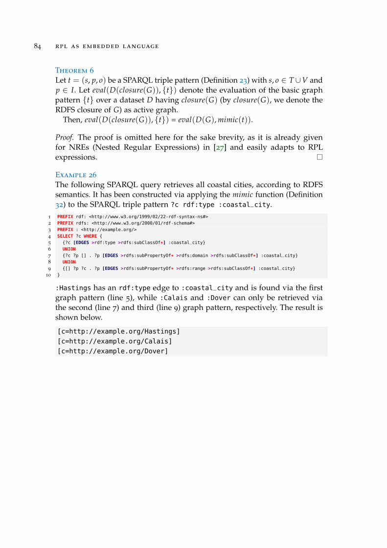
84 rpl as embedded language
Theorem 6
Let t = (s, p, o) be a SPARQL triple pattern (Definition 23) with s, o ∈ T∪V andp ∈ I. Let eval(D(closure(G)), t) denote the evaluation of the basic graphpattern t over a dataset D having closure(G) (by closure(G), we denote theRDFS closure of G) as active graph.
Then, eval(D(closure(G)), t) = eval(D(G), mimic(t)).
Proof. The proof is omitted here for the sake brevity, as it is already givenfor NREs (Nested Regular Expressions) in [27] and easily adapts to RPLexpressions.
Example 26
The following SPARQL query retrieves all coastal cities, according to RDFSsemantics. It has been constructed via applying the mimic function (Definition32) to the SPARQL triple pattern ?c rdf:type :coastal_city.
1 PREFIX rdf: <http://www.w3.org/1999/02/22-rdf-syntax-ns#>
2 PREFIX rdfs: <http://www.w3.org/2000/01/rdf-schema#>
3 PREFIX : <http://example.org/>
4 SELECT ?c WHERE
5 ?c [EDGES >rdf:type >rdfs:subClassOf*] :coastal_city
6 UNION
7 ?c ?p [] . ?p [EDGES >rdfs:subPropertyOf* >rdfs:domain >rdfs:subClassOf*] :coastal_city
8 UNION
9 [] ?p ?c . ?p [EDGES >rdfs:subPropertyOf* >rdfs:range >rdfs:subClassOf*] :coastal_city
10
:Hastings has an rdf:type edge to :coastal_city and is found via the firstgraph pattern (line 5), while :Calais and :Dover can only be retrieved viathe second (line 7) and third (line 9) graph pattern, respectively. The result isshown below.
[c=http://example.org/Hastings]
[c=http://example.org/Calais]
[c=http://example.org/Dover]

5E X P E R I M E N TA L E VA L U AT I O N
This chapter presents RPLgen (Section 5.1), an RDF data generator based onRPL queries. It is able to create richly structured, path-based RDF data, and hasbeen applied to generate the datasets (Section 5.2) for experimentally verifyingthe complexity bounds of all presented evaluation algorithms (Section 5.3).
5.1 R P L G E N – G E N E R AT I N G R D F D ATA F R O M R P L Q U E R I E S
Each RPL query describes a certain set of paths within an RDF graph. The newview that RPLgen brings into play is to interpret these paths in a generativeway, i.e. materialize some of them into RDF data.
For instance, the RPL query q
1 PATH :Paris
2 ( >[PATH (:bus | :ferry | :train) >rdfs:subPropertyOf :transport]
3 :/city[0-9]+/
4 )+
generates an RDF graph similar to the one from Figure 6, as it describes a pathp of non-zero length. The first node of p is :Paris (line 1), while all followingnodes are labeled with :city followed by an arbitrary, non-empty sequenceof digits (indicated by :/city[0-9]+/ in line 3). All edges of p have to satisfypaths p′, which are described by the predicate in line 2. However, each p′ is apath of length one, starting with a node either labeled :bus, :ferry, or :train,which is connected to a :transport node via an rdfs:subPropertyOf edge.
The RPL query q presented above can indeed be used as an input forRPLgen. Figure 20 shows the resulting RDF graph, when calling RPLgen withone instance of q, a success probability of 0.3 and an initial seed of 98765 (theseparameters are described in the following).
85

86 experimental evaluation
:ferry
rdfs:sp rdfs:sp
:bus
:bus :train
rdfs:sp
:transport
:Paris :city115 :city6 :city09857860:ferry :train
Figure 20: An example RDF graph created by RPLgen
RPLgen is an RDF data generator that is based on using RPL queries in agenerative way. An important idea has been adopted from the SP2 BenchGenerator1, an RDF data generator for DBLP-like data: repeatability, i.e. whencalled with the same parameters, the same data will be generated.
Hence, the first of RPLgen’s parameters is a seed value to initialize the randomnumber generator. When RPLgen is run several times with identical seed,each single “randomized” decision is deterministic and will lead to the sameoutcome — thus, the generated data will be identical as well.
The second parameter that RPLgen requires is a success probability p, whichcontrols how often Kleene star and plus operators are expanded. This appliesto regular expressions over strings (used in AtomicRPEs), as well as for themultiplicities within RPL expressions (used in AdornedRPEs).
More precisely, the probability that a Kleene star operator is expandedk times is given by Gp(k) in the probability space (N, 2N,Gp), where 2N
denotes the power set of N. Gp is called the geometric distribution [18] withparameter p and is defined as Gp(k) := p(1− p)k.
In case of a Kleene plus operator, we just need to shift Gp one unit to theright. So, the probability that a Kleene plus operator is expanded k times isgiven by Gp(k− 1) = p(1− p)k−1.
However, the application of the geometric distribution is limited to Kleenestar and plus operators – all remaining random decisions range over a finiteset of alternatives, and each of these alternatives should obtain the sameprobability (leading to a uniform distribution).
RPLgen’s third parameter is a list of RPL queries, where each query q isequipped with a number stating how many instances of q are to be generated.
1 see http://dbis.informatik.uni-freiburg.de/index.php?project=SP2B/data.php

5.1 rplgen – generating rdf data from rpl queries 87
Example 27
This example gives a lookup table for the geometric distribution with parame-ters p = 0.1 and p = 0.2.
k 0 1 2 3 4 5
G0.1(k) 0.1 0.09 0.081 0.0729 0.06561 0.05905G0.2(k) 0.2 0.16 0.128 0.1024 0.08192 0.06554
As already mentioned, regular expressions occur at two levels: a RPL expres-sion itself can be interpreted as a regular expression, as well as all of its atomicsubexpressions. The implementation of these two levels is discussed in thefollowing Sections 5.1.1 and 5.1.2.
5.1.1 Regular Expressions over Strings
RPLgen has to do some preprocessing concerning regular expressions overstrings, the lower of these two levels. The dk.brics.automaton implementation[24] represents regular expressions as a binary tree (i.e. each node must nothave more than two children). If a regular expression contains more than twoalternatives (at any depth), not of all of these will be at the same level withinits abstract syntax tree. This representation is quite uncomfortable since eachof these alternatives should be chosen with the same probability. So, beforegenerating strings from regular expressions, the latter have to be flattenedby translating them into a tree structure where each node can have arbitrarymany children.
The AtomicRPE _ (the wildcard) matches each node or edge label and thuscan be seen as the regular expression .*, where . matches any character fromthe character classes [a-z], [A-Z], and [0-9].
5.1.2 RPL Queries as Regular Expressions
In contrast, no further preprocessing of RPL queries is required, as these arealready “flattened” after the simplification pass (Section 3.1.1).
RPL predicates with a negative sign ([!. . .]) are, when using them in agenerative way like RPLgen does, treated as if they carried a positive sign.Otherwise, it would be unclear which part of the predicate the user hasintended to fail.

88 experimental evaluation
When a PredicatesRPE is made up of multiple PredicateRPEs p1, . . . , pn(n ≥ 2), only p1 is guaranteed to be satisfied when evaluating its parentRPL query. The semantics of RPL actually defines that all predicates p1, . . . , pnshould be satisfied, but this would have meant a lot of additional programmingeffort. The intersection of two regular expressions r1, r2 (which could representthe first atomic expressions of p1 and p2) is usually computed by converting r1and r2 into NFAs A1 and A2, which in turn are determinised into DFAs D1and D2, and combined into a product automaton P that accepts the languageL(r1) ∩ L(r2). Finally, P would have to be converted back into a regularexpression r, which allows for usage in a generative way.
5.2 E VA L U AT I O N S E T U P
Before presenting its results in Section 5.3, we need to concisely describe thesetup of the experimental evaluation.
Therefore, we present the query that is used both as an input for RPLgenand later for querying the generated datasets (Section 5.2.1).
Moreover, a little pseudo code fragment illustrates how time measurementis conducted (Section 5.2.2).
5.2.1 Data Generation
The generated data has a similar structure as the introductory example fromFigure 20. More precisely, RPLgen is initialized with the following RPL query.
1 PATH :/c[0-9]+/
2 ( >[PATH (:/t[0-9]+/ >rdfs:subPropertyOf)* :transport]
3 :/c[0-9]+/
4 )+
Listing 9: RPL query serving as input for RPLgen
This query q describes a path of non-zero length, where each node shouldrepresent a city and is labeled with :/c[0-9]+/ (c followed by an arbitrary,non-empty sequence of digits, see line 3). Each edge of the path representsa transportation service and has to satisfy a predicate q′, which describes apath consisting of zero or more >rdfs:subPropertyOf edges that finally reacha node labeled :transport (line 2). Each node of q′ (except the last one) islabeled with :/t[0-9]+/ (t followed by an arbitrary, non-empty sequence ofdigits, see line 2).
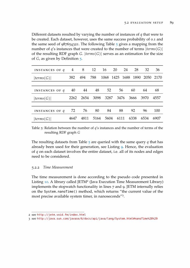
5.2 evaluation setup 89
Different datasets resulted by varying the number of instances of q that were tobe created. Each dataset, however, uses the same success probability of 0.1 andthe same seed of 987654321. The following Table 5 gives a mapping from thenumber of q’s instances that were created to the number of terms |terms(G)|of the resulting RDF graph G. |terms(G)| serves as an estimation for the sizeof G, as given by Definition 5.
instances of q 4 8 12 16 20 24 28 32 36
|terms(G)| 382 494 788 1068 1425 1688 1890 2050 2170
instances of q 40 44 48 52 56 60 64 68
|terms(G)| 2262 2654 3098 3287 3476 3666 3970 4557
instances of q 72 76 80 84 88 92 96 100
|terms(G)| 4647 4811 5164 5604 6111 6338 6534 6907
Table 5: Relation between the number of q’s instances and the number of terms of theresulting RDF graph G
The resulting datasets from Table 5 are queried with the same query q that hasalready been used for their generation, see Listing 9. Hence, the evaluationof q on each dataset involves the entire dataset, i.e. all of its nodes and edgesneed to be considered.
5.2.2 Time Measurement
The time measurement is done according to the pseudo code presented inListing 10. A library called JETM2 (Java Execution Time Measurement Library)implements the stopwatch functionality in lines 7 and 9. JETM internally relieson the System.nanoTime() method, which returns “the current value of themost precise available system timer, in nanoseconds”3.
2 see http://jetm.void.fm/index.html3 see http://java.sun.com/javase/6/docs/api/java/lang/System.html#nanoTime%28%29

90 experimental evaluation
The MEASUREMENT procedure from Listing 10 is called with all datasets fromTable 5, the RPL query string from Listing 9, and 25 iterations. During theseiterations, JETM collects all stopwatch times and calculates the minimum, aver-age, and maximum run times for each dataset and each evaluation approach:the ENRE-based evaluation (Section 3.3) and the two variants of the Path-basedevaluation (Section 3.4).
procedure MEASUREMENT(File[] dataset, String query, int iterations)1 run once each evaluation approach of query on dataset[0]2 for each dataset[i]3 for each evaluation approach approach4 for each iteration5 create graph G from dataset[i]6 parse q from the query string query7 start stopwatch
8 evaluate q on G via approach9 stop stopwatch
Listing 10: Pseudo code for time measurement
The first line of Listing 10 ensures that the very first measurement for eachevaluation approach is not affected by any classloading times. To preventmemoization from taking place beyond different iterations (line 4), a newinstance of an RDF graph is generated from the current dataset and the querystring is parsed into a new RPL query at the beginning of each iteration(compare lines 5 – 6).
The time measurement has been carried out on an Intel Pentium Dual CoreCPU T2330, with each core clocked at 1.60 GHz. A 64-bit edition of the JavaDevelopment Kit, version 1.6.0_17, was run with an initial and maximumheap size of 1.5 GB (by the command line switches -Xms1536m and -Xmx1536m,respectively).
5.3 R E S U LT S
The (average) resulting run times measured by JETM under the setup describedin the previous section are shown in Figure 21.
The upper diagram contains all values that were captured during the ENRE-based evaluation of the RPL query from Listing 9 on all datasets from Table 5.As the ENRE-based approach is shown to have a time complexity quadratic

5.3 results 91
in the size of the data (Section 3.3.4), a quadratic polynomial is fitted to theacquired values.
Similarly, the lower diagram contains all values that were captured for bothvariants of the Path-based evaluation. The first series of measurements refers tothe algorithm from Section 3.4.2, the first variant of the Path-based evaluation,for which an exponential upper bound has been shown in Section 3.4.3. Thesecond series of measurements refers to the second variant of the Path-basedevaluation (Section 3.4.4), for which cubic data time complexity has beenshown. Similar to the upper diagram, a cubic polynomial is fitted to each seriesof measurements.
Figure 21 hence experimentally verifies the shown time complexity boundsfor all of the presented evaluation approaches. Furthermore, it depicts thatthe first variant of the Path-based evaluation (Section 3.4.2) seems to alsohave a time complexity that is cubic in the size of the data, although only anexponential upper bound has been formulated in this thesis (Theorem 4).
When comparing the upper and lower diagrams of Figure 21 with eachother, keep in mind that the unit of the vertical axis in the upper diagramis milliseconds, while it is seconds in the lower diagram. Even though ENRE-based evaluation outperforms Path-based evaluation on large enough datasets,the latter approach might be favorable if (1) it benefits from its memoizationapproach, e.g. when a RPL query is evaluated more than once in embeddedmode, and the bindings of imported SPARQL variables change in between(compare Section 4.3), and (2) the selectivity of a RPL query is higher than onthe generated datasets.

92 experimental evaluation
0
500
1000
1500
2000
2500
3000
3500
4000
4500
5000
0 1000 2000 3000 4000 5000 6000 7000
time
[ms]
dataset size [number of RDF terms]
ENRE-based evaluationfitted quadratic polynomial
0
500
1000
1500
2000
2500
3000
3500
0 1000 2000 3000 4000 5000 6000 7000
time
[s]
dataset size [number of RDF terms]
first variant of Path-based evaluationfitted cubic polynomial
second variant of Path-based evaluationfitted cubic polynomial
Figure 21: The two diagrams show the resulting run times of the RPL query fromListing 9 on all datasets from Table 5. The ENRE-based run times are shownin the upper, the Path-based run times (for both variants) in the lowerdiagram.

6L E A R N I N G R P L
This chapter briefly presents three tools that have been created for learningRPL and to ease the authoring of RPL expressions. All tools (the web-basedinterface presented in Section 6.1, and the two Eclipse plugins presented inSections 6.2 and 6.3) are available online at http://rpl.pms.ifi.lmu.de/.
6.1 W E B - B A S E D I N T E R FA C E
The web-based interface of RPL is targeted at users willing to cast an eye overRPL. It includes two application scenarios (named Transport and FOAF, likethe FOAF vocabulary1), each consisting of an RDF dataset along with severalpredefined RPL queries, as shown in Figure 22.
Clicking the Submit Query button submits the blue form in the upper halfof Figure 22 via an AJAX POST request. At the server side, a single servletprocesses the incoming request, and sends back a response, encoded in XML.In the absence of errors, this response consists of the simplified and normal-ized RPL query, its corresponding ENRE (along with the time required fortranslation), and the result of the evaluation (again along with its requiredtime), as shown in Figure 23. Otherwise, an error dialog containing a messagelike those shown in Section 3.1 appears.
This web-based interface can be easily deployed on any Java servlet engine(e.g. Apache Tomcat2) by installing a single web archive file, which in turncan be built via Apache Ant3. User interaction and AJAX communication onclient side are built on top of a javascript framework called jQuery4. RPL’sweb-based interface has been tested to work with any modern browser.
1 see http://www.foaf-project.org/2 see http://tomcat.apache.org/3 see http://ant.apache.org/4 see http://jquery.com/
93

94 learning rpl
Figure 22: Screenshot of RPL’s web-based interface

6.2 visrpl – a visual editor for rpl 95
Figure 23: Response of the web-based interface, when evaluating the RPL queryEDGES >[PATH (_ >rdfs:subPropertyOf)* :transport]+ on the Transportdataset shown in Figures 6 and 22
6.2 V I S R P L – A V I S U A L E D I T O R F O R R P L
The idea of creating visRPL, a visual editor for RPL, was born during the finalpresentation of visKWQL [19].
When designing a visual editor for an arbitrary (textual) programmingor query language, one crucial challenge is to find a visual model for thatlanguage that is as expressive as the textual language itself (i.e. each textualquery should be expressible by a visual query and the other way round), andstill convenient to work with for the user. Simply building a visual editor byhave the user “draw” an abstract syntax tree of a textual query would certainlynot lead to any gain over a textual editor.
Concerning visRPL, this visual model consists of boxes that can be nested intoone another, as shown in Figure 24. A Composite box, for instance, combinesthe expressivity of an AdornedRPE (by a multiplicity value located in its upperright corner), a DisjunctiveRPE (by allowing several alternate paths withinitself) and a ConcatenatedRPE (by allowing several child boxes on each path).
The connectors (the red lines in Figure 24) run from left to right within eachbox, and thus visually describe its paths. For instance, the outermost Flavoredbox in Figure 24 defines only one path, consisting of an Atomic box (the one

96 learning rpl
containing the string “:Paris”) followed by a Composite box (the one whosemultiplicity in the upper right corner is about to be changed via the showndrop-down menu). This Composite box in turn defines a path, now consisting ofa Predicates box (highlighted in green) that is connected to another Atomic box.However, the multiplicity + of this Composite box tells us that we are allowedto run through its inner path(s) for an arbitrary, non-zero number of times.
The lower part of Figure 24 shows the RPL Query View, which contains atextual query that corresponds to the visual query shown in the editor above.As textual and visual RPL queries have the same expressivity, roundtripping[19] is possible in both directions. Roundtripping can either be manuallyinitiated via the Generate Diagram and Generate Query buttons, or automaticallybe run each time when the textual or visual query is changed by the user (thiscan be enabled via the Synchronize checkbox).
Figure 24: Screenshot of visRPL
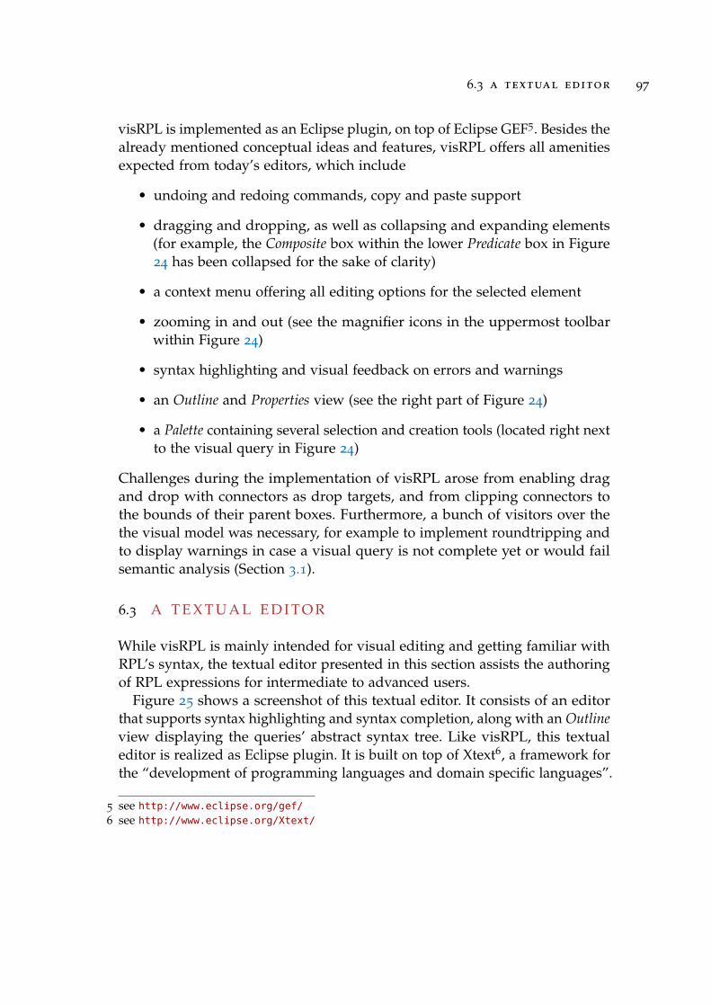
6.3 a textual editor 97
visRPL is implemented as an Eclipse plugin, on top of Eclipse GEF5. Besides thealready mentioned conceptual ideas and features, visRPL offers all amenitiesexpected from today’s editors, which include
• undoing and redoing commands, copy and paste support
• dragging and dropping, as well as collapsing and expanding elements(for example, the Composite box within the lower Predicate box in Figure24 has been collapsed for the sake of clarity)
• a context menu offering all editing options for the selected element
• zooming in and out (see the magnifier icons in the uppermost toolbarwithin Figure 24)
• syntax highlighting and visual feedback on errors and warnings
• an Outline and Properties view (see the right part of Figure 24)
• a Palette containing several selection and creation tools (located right nextto the visual query in Figure 24)
Challenges during the implementation of visRPL arose from enabling dragand drop with connectors as drop targets, and from clipping connectors tothe bounds of their parent boxes. Furthermore, a bunch of visitors over thethe visual model was necessary, for example to implement roundtripping andto display warnings in case a visual query is not complete yet or would failsemantic analysis (Section 3.1).
6.3 A T E X T U A L E D I T O R
While visRPL is mainly intended for visual editing and getting familiar withRPL’s syntax, the textual editor presented in this section assists the authoringof RPL expressions for intermediate to advanced users.
Figure 25 shows a screenshot of this textual editor. It consists of an editorthat supports syntax highlighting and syntax completion, along with an Outlineview displaying the queries’ abstract syntax tree. Like visRPL, this textualeditor is realized as Eclipse plugin. It is built on top of Xtext6, a framework forthe “development of programming languages and domain specific languages”.
5 see http://www.eclipse.org/gef/6 see http://www.eclipse.org/Xtext/

98 learning rpl
Figure 25: Screenshot of RPL’s textual editor
Unfortunately, Xtext internally applies ANTLRv3, whose lexer component isunable to decide whether a < character in the input stream marks the beginningof an 〈IRI_REF〉 token (e.g. <http://example.org>, see Definition 1), or is usedas a direction modifier. This drawback of ANTLRv3 is already discussed inSection 2.3, and leads to an error message like shown in Figure 26 within thetextual editor.
As a workaround, the generated Java lexer classes have been manuallymodified such that whenever an 〈IRI_REF〉 token is to be matched, it is earlychecked if this match will succeed — without consuming any charactersfrom the input stream yet. If this check is successful, an 〈IRI_REF〉 token willbe emitted; otherwise, < will be interpreted as direction modifier. Figure 27
demonstrates the success of this workaround.However, this workaround has to be reapplied, if the RPL syntax is about
to change in the future, as the concerning Java lexer files will have to beregenerated from an Xtext grammar file.

6.3 a textual editor 99
Figure 26: Screenshot of the textual editor for RPL, demonstrating ANTLRv3’s lexerweakness. As can be seen in the Problems view, the < character was inter-preted as the beginning of an 〈IRI_REF〉 token (which is expected to endwith a > character)
Figure 27: Same screenshot as in Figure 26, after the workaround has been applied. Itis shown in the Outline view, that the < character is now correctly recognizedas direction modifier


7R E L AT E D W O R K
SPARQL’s lack of navigational capabilities has led to the development of aplethora of SPARQL extensions like SPARQLeR [22], (C)PSPARQL [2], andnSPARQL [27].
Since RPL has already been compared to all of these extensions in [9], onlyone new aspect shall be contributed here. In Chapter 3, ENREs have beenintroduced as an extension of NREs (Nested Regular Expressions), whichform the basis of nSPARQL. However, ENREs have been tailored to fit thepeculiarities of RPL, and extend (by allowing regular expressions as label tests,some new navigation axes, and the negation of nested expressions) but at thesame time limit NREs (by abandoning their navigation axes node and edge,together with their inverse axes node−1 and edge−1, respectively).
The concept of navigation axes arguably helped a lot to turn XPath [11] intoits huge success, and has been borrowed for NREs, whose navigation axes areshown in Figure 28.
edge-1
b aa
p p
b
edge node
next next-1
node-1
Figure 28: Navigational axes for an RDF triple (a, p, b), as presented in [27]
In the following, we demonstrate that the additional axes that NREs offer canbe expressed via query rewriting, when RPL is used in embedded mode.
In Figure 29, the path from ?a to ?b (highlighted in maroon) and the pathfrom ?d to ?e (highlighted in blue) should be in the evaluation of the NREs α
and β, respectively. α and β should furthermore not contain any navigationaxis from the set node, node−1, edge, edge−1.
101

102 related work
The NRE α/edge:::c/β (denoted by γ) defines a path from ?a to ?e (itsendpoints are highlighted with green background). Note that this “path” isnot a path in the sense of Definition 4, so it can not be queried by an ENREnor a RPL query1.
:c?a ?b
?d
?e
?d. . .
..
.
1
Figure 29: Expressivity of NREs and ENREs
However, when using RPL inside of SPARQL, this lack of expressivity can becompensated by two RPL triple patterns expressing the NREs α and β, andone SPARQL triple pattern expressing the edge:::c move, as shown in thesnippet below.
SELECT ?a ?e WHERE ?a [q1] ?b . ?b ?d :c . ?d [q2] ?e
This shows that RPL indeed avoids reinventing the wheel, and reuses thefunctionality already provided by SPARQL. Although similar for the remainingaxes edge−1, node, and node−1, this rewriting can only be done a finite numberof times; the result, however, is an acyclic SPARQL basic graph pattern andcan be efficiently evaluated [16]. If, for instance, an edge axis is enclosed inan outer Kleene star or Kleene plus operator, this would lead to an infinitenumber of SPARQL triple patterns (one is required for each possible edge
move) and thus to a SPARQL query of infinite length. So, in this case, thegain of expressivity from SPARQL is not big enough to fully incorporate theadditional axes available for NREs.
1 When using a RPL predicate for the path from ?d to ?e, only the pair (?a, : c) would be in theevaluation of the resulting query, in contrast to the evaluation of γ, which contains pairs ofthe form (?a, ?e).

8C O N C L U S I O N A N D F U RT H E R W O R K
Concluding, this work presents a refined version of RPL’s syntax and semantics.The graph labeling algorithm for the evaluation of nSPARQL’s nested regularexpressions [27] has been extended to fit the peculiarities of RPL, withoutincreasing its time complexity of O(|G|2 · |q|). Furthermore, a novel evaluationapproach is introduced: it stores a matrix along with each subexpression eof a RPL query, holding (the endpoints of) all paths satisfying e. Thoughthis approach has time complexity O(|G|3 · |q|), it can be beneficial on smalldatasets and when using RPL in embedded mode, as part of these matricesmight be reused. It has been shown that RPL is able to imitate the RDFSsemantics when using SPARQL as host language. An entire tool suite for RPLis developed in this thesis: (1) a RPL-based RDF data generator named RPLgen,which has already been applied during the experimental evaluation, (2) aweb-based interface for seeing RPL in action, and (3) visRPL, an Eclipse pluginallowing to graphically compose RPL queries.
In the following, we point out some of the remaining open issues, groupedinto four categories.
RPL Language
Compared to the NREs (Nested Regular Expressions) of nSPARQL [27], RPLis not able to express node and edge moves (and their inverse moves node−1
and edge−1, respectively), as illustrated in Chapter 7. It could be checked, ifRPL (and its evaluation algorithms) can be extended to fully incorporate theexpressivity of NREs.
Another open question concerning the expressivity of RPL is the following: IsRPL’s expressivity, after having it extended to incorporate the full expressivityof NREs as described above, already at the limit concerning the expressivity of
103

104 conclusion and further work
RDF path languages that can be evaluated in time O(|G|2 · |q|), or might therebe any further interesting language extensions whose time complexity stayswithin that bound?
RPL Evaluation
As shown in Section 3.4.4, the time complexity of the second variant of thePath-based evaluation is cubic in the size of the queried RDF graph. However,its memoization technique is a beneficial approach, in particular when RPLis used in embedded mode and imports variables from its host language. Itcould be analysed, if this memoization technique can also be applied to theENRE-based evaluation, ideally without increasing its time complexity.
Both evaluation approaches (ENRE-based and Path-based evaluation, seeSections 3.3 and 3.4) presented in this thesis are based on a RAM model. It canbe further investigated, if indexing techniques allow for an efficient disk-basedevaluation of RPL, and how these algorithms would have to be adapted.
The recent spreading of multi-core and networked environments gives rise toanother interesting research approach: the parallelization of RPL’s evaluation.Google’s MapReduce [14] (together with its open source implementationApache Hadoop1) might serve as a starting point here.
RPLgen
RPLgen, the RPL-based RDF data generator presented in Section 5.1, can befurther extended such that each predicate within a PredicatesRPE is satisfiedon the generated data (currently, this is only the case for the first predicate).
visRPL
visRPL, the visual editor for RPL queries presented in Section 6.2, can beextended to not only cover the construction, but also the evaluation of RPLqueries — either directly against RDF data in standalone mode or againstthe storage interfaces provided by a SPARQL framework when using RPLin embedded mode. This, at the same time, would be visRPL’s first stepfrom a standalone visual editor towards a comprehensive IDE (IntegratedDevelopment Environment) for RPL.
1 see http://hadoop.apache.org/

AA P P E N D I X
a.1 P R O O F O F T H E O R E M 2
Proof. We use structural induction over RPEs and start with the base case,which is AtomicRPE. The notation used within the following boxes is explainedin Section 2.2.2.
Let a be an AtomicRPE, pos := a.getPosition(), rx := a.getRegExp().Case pos = NODE
[[[a]]]G = (n, n) | ∃n ∈ nodes(G) ∧ n ∈ L(rx) (Def 9)= Jself_node::rxKG = Jtrans(a)KG (Def 11, 13)
Case pos = EDGE
[[[a]]]FORWARDG = (s, o) | ∃p : (s, p, o) ∈ G ∧ p ∈ L(rx) (Def 9)
= Jnext::rxKG = JtransFORWARD(a)KG (Def 11, 13)
[[[a]]]BACKWARDG = (o, s) | (s, o) ∈ [[[a]]]FORWARDG (Def 9)= (o, s) | (s, o) ∈ Jnext::rxKG (I.H.)
= Jnext−1::rxKG = JtransBACKWARD(a)KG (Def 11, 13)
[[[a]]]UNDIRECTEDG = [[[a]]]FORWARDG ∪ [[[a]]]BACKWARDG (Def 9)= Jnext::rxKG ∪ Jnext−1::rxKG (I.H.)= Jnext_or_next−1::rxKG (Def 11)
= JtransUNDIRECTED(a)KG (Def 13)
105

106 appendix
Let p be a PredicateRPE, f := p.getFlavored(), pos := p.getPosition(), andsign := p.getSign().Case pos = NODE, sign = POSITIVE
[[[p]]]G = (n, n) | n ∈ nodes(G) ∧ ∃q : (n, q) ∈ [[[ f ]]]G (Def 9)= (n, n) | n ∈ nodes(G) ∧ ∃q : (n, q) ∈ Jtrans( f )KG (I.H.)= Jself_node::[trans( f )]KG = Jtrans(p)KG (Def 11, 13)
Case pos = NODE, sign = NEGATIVE
Like the POSITIVE case, just replace ∃ with @ and self_node::[trans( f )]with self_node::![trans( f )].
Case pos = EDGE, sign = POSITIVE
[[[p]]]G = (e, e) | e ∈ edges(G) ∧ ∃q : (e, q) ∈ [[[ f ]]]G (Def 9)= (e, e) | e ∈ edges(G) ∧ ∃q : (e, q) ∈ Jtrans( f )KG (I.H.)= Jself_edge::[trans( f )]KG = Jtrans(p)KG (Def 11, 13)
Case pos = EDGE, sign = NEGATIVE
Like the POSITIVE case, just replace ∃ with @ and self_edge::[trans( f )]with self_edge::![trans( f )].
Let p be a PredicatesRPE, p1, p2, . . . , pn (n ≥ 1) its children, pos := p.getPosition().Case pos = NODE
[[[p]]]G= (n, n) | n ∈ nodes(G) ∧ (n, n) ∈ [[[p1]]]G . . . [[[pn]]]G (Def 9)= (n, n) | n ∈ nodes(G) ∧ ∃q : (n, q) ∈ [[[p1]]]G . . . [[[pn]]]G (*)= (n, n) | n ∈ nodes(G) ∧ ∃q : (n, q) ∈ Jtrans(p1)KG . . . Jtrans(pn)KG (I.H.)= (n, n) | n ∈ nodes(G) ∧ ∃q : (n, q) ∈ Jtrans(p1)/. . ./trans(pn)KG (Def 11)= Jself_node::[trans(p1)/. . ./trans(pn)]KG = Jtrans(p)KG (Def 11, 13)
Case pos = EDGE
[[[p]]]FORWARDG
= (s, o) | ∃(s, e, o) ∈ G ∧ (e, e) ∈ [[[p1]]]G . . . [[[pn]]]G (Def 9)= (s, o) | ∃(s, e, o) ∈ G ∧ ∃q : (e, q) ∈ [[[p1]]]G . . . [[[pn]]]G (*)= (s, o) | ∃(s, e, o) ∈ G ∧ ∃q : (e, q) ∈ Jtrans(p1)KG . . . Jtrans(pn)KG (I.H.)= (s, o) | ∃(s, e, o) ∈ G ∧ ∃q : (e, q) ∈ Jtrans(p1)/. . ./trans(pn)KG (Def 11)
= Jnext::[trans(p1)/. . ./trans(pn)]KG = JtransFORWARD(p)KG (Def 11, 13)
The remaining cases [[[p]]]BACKWARDG and [[[p]]]UNDIRECTEDG can be done similar as for AtomicRPEs.(*): As each [[[pi]]]G (1 ≤ i ≤ n) just contains symmetric pairs (x, y) where x = y, thisalso applies for [[[p1]]]G . . . [[[pn]]]G.
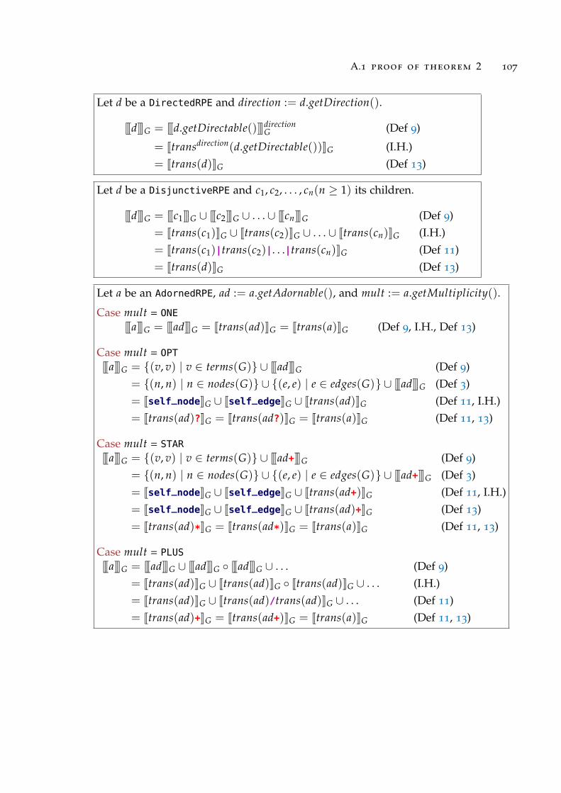
A.1 proof of theorem 2 107
Let d be a DirectedRPE and direction := d.getDirection().
[[[d]]]G = [[[d.getDirectable()]]]directionG (Def 9)
= Jtransdirection(d.getDirectable())KG (I.H.)= Jtrans(d)KG (Def 13)
Let d be a DisjunctiveRPE and c1, c2, . . . , cn(n ≥ 1) its children.
[[[d]]]G = [[[c1]]]G ∪ [[[c2]]]G ∪ . . . ∪ [[[cn]]]G (Def 9)= Jtrans(c1)KG ∪ Jtrans(c2)KG ∪ . . . ∪ Jtrans(cn)KG (I.H.)= Jtrans(c1)|trans(c2)|. . .|trans(cn)KG (Def 11)= Jtrans(d)KG (Def 13)
Let a be an AdornedRPE, ad := a.getAdornable(), and mult := a.getMultiplicity().
Case mult = ONE
[[[a]]]G = [[[ad]]]G = Jtrans(ad)KG = Jtrans(a)KG (Def 9, I.H., Def 13)
Case mult = OPT
[[[a]]]G = (v, v) | v ∈ terms(G) ∪ [[[ad]]]G (Def 9)= (n, n) | n ∈ nodes(G) ∪ (e, e) | e ∈ edges(G) ∪ [[[ad]]]G (Def 3)= Jself_nodeKG ∪ Jself_edgeKG ∪ Jtrans(ad)KG (Def 11, I.H.)= Jtrans(ad)?KG = Jtrans(ad?)KG = Jtrans(a)KG (Def 11, 13)
Case mult = STAR
[[[a]]]G = (v, v) | v ∈ terms(G) ∪ [[[ad+]]]G (Def 9)= (n, n) | n ∈ nodes(G) ∪ (e, e) | e ∈ edges(G) ∪ [[[ad+]]]G (Def 3)= Jself_nodeKG ∪ Jself_edgeKG ∪ Jtrans(ad+)KG (Def 11, I.H.)= Jself_nodeKG ∪ Jself_edgeKG ∪ Jtrans(ad)+KG (Def 13)= Jtrans(ad)*KG = Jtrans(ad*)KG = Jtrans(a)KG (Def 11, 13)
Case mult = PLUS
[[[a]]]G = [[[ad]]]G ∪ [[[ad]]]G [[[ad]]]G ∪ . . . (Def 9)= Jtrans(ad)KG ∪ Jtrans(ad)KG Jtrans(ad)KG ∪ . . . (I.H.)= Jtrans(ad)KG ∪ Jtrans(ad)/trans(ad)KG ∪ . . . (Def 11)= Jtrans(ad)+KG = Jtrans(ad+)KG = Jtrans(a)KG (Def 11, 13)

108 appendix
Let c be a ConcatenatedRPE and a1, a2, . . . , an(n ≥ 1) its children.
[[[c]]]G = [[[a1]]]G [[[a2]]]G . . . [[[an]]]G (Def 9)= Jtrans(a1)KG Jtrans(a2)KG . . . Jtrans(an)KG (I.H.)= Jtrans(a1)/trans(a2)/. . ./trans(an)KG (Def 11)= Jtrans(c)KG (Def 13)
Let f be a FlavoredRPE and c := f .getConcatenated().
[[[ f ]]]G = [[[c]]]G = Jtrans(c)KG = Jtrans( f )KG (Def 9, I.H., Def 13)
a.2 TA R J A N ’ S A L G O R I T H M
Tarjan’s algorithm identifies strongly connected components in directed graphsG = (V, E). The pseudo code presented here consists of several global vari-ables, a TARJAN method to be called by the user after G has been set, and aSTRONGCONNECT method that is called once on every node v ∈ V of G. Thispresentation is based on [31] as well as [23].
The correctness of this algorithm is shown in [31]. Furthermore, it is shownto have a time bound of O(|V|+ |E|), if the open stack (a global variable) isadditionally represented as a boolean array of size |V|, such that it can betested in constant time whether a node is on the open stack or not.
index an integer
G = (V, E) a directed graph
open a stack over Vnumber, lowlink arrays of integers over V
procedure TARJAN()
index := 0for each v ∈ V
number[v] := 0open := empty stack
for each v ∈ Vif number[v]= 0STRONGCONNECT(v)

A.2 tarjan’s algorithm 109
procedure STRONGCONNECT(v)lowlink[v] := number[v] := ++indexopen.push(v)for each w ∈ V with (v, w) ∈ Eif number[w] = 0STRONGCONNECT(w)
lowlink[v] := min(lowlink[v], lowlink[w])else if w ∈ open // can be done in O(1)
lowlink[v] := min(lowlink[v], number[w])if lowlink[v] = number[v]start new strongly connected component
repeat
u := open.pop()add u to the current component
until u = v


B I B L I O G R A P H Y
[1] Serge Abiteboul, Richard Hull, and Victor Vianu. Foundations of Databases.Addison-Wesley, 1995. ISBN 0-201-53771-0. (Cited on pages 35 and 52.)
[2] Faisal Alkhateeb, Jean-François Baget, and Jérôme Euzenat. ExtendingSPARQL with regular expression patterns (for querying RDF). WebSemantics: Science, Services and Agents on the World Wide Web, 7(2):57 – 73,2009. (Cited on page 101.)
[3] Renzo Angles and Claudio Gutierrez. The Expressive Power of SPARQL.In International Semantic Web Conference, Lecture Notes in Computer Sci-ence, pages 114–129. Springer, 2008. http://www.dcc.uchile.cl/TR/
2006/TR_DCC-2006-009.pdf. (Cited on page 75.)
[4] Grigoris Antoniou and Frank van Harmelen. A Semantic Web Primer. MITPress, 2008. ISBN 978-0-262-01242-3. (Cited on page 1.)
[5] Jean-François Baget. RDF Entailment as a Graph Homomorphism.In International Semantic Web Conference, Lecture Notes in ComputerScience, pages 82–96. Springer, 2005. http://www.lirmm.fr/~baget/
publications/ISWC05.pdf. (Cited on page 17.)
[6] Dave Beckett. RDF/XML Syntax Specification (Revised). Rec-ommendation, W3C, February 2004. http://www.w3.org/TR/2004/
REC-rdf-syntax-grammar-20040210/. (Cited on page 17.)
[7] Dave Beckett and Tim Berners-Lee. Turtle - Terse RDF Triple Lan-guage, W3C Team Submission, 2008. Online only. http://www.w3.org/TeamSubmission/turtle/, retrieved at 2010/01/01. (Cited on page 17.)
[8] Jeen Broekstra, Arjohn Kampman, and Frank van Harmelen. Sesame: AGeneric Architecture for Storing and Querying RDF and RDF Schema.In International Semantic Web Conference, Lecture Notes in Computer Sci-ence, pages 54–68. Springer, 2002. http://www.openrdf.org/doc/papers/Sesame-ISWC2002.pdf. (Cited on pages 73 and 77.)
111

112 bibliography
[9] François Bry, Tim Furche, and Benedikt Linse. The PerfectMatch: RPL and RDF Rule Languages. In Web Reasoning andRule Systems, Lecture Notes in Computer Science, pages 227–241.Springer, 2009. http://www.pms.ifi.lmu.de/publikationen/PMS-FB/
PMS-FB-2009-9/PMS-FB-2009-9-paper.pdf. (Cited on pages 4, 5, 9, 14,33, 49, 83, and 101.)
[10] Jeremy J. Carroll and Graham Klyne. Resource Description Framework(RDF): Concepts and Abstract Syntax. Recommendation, W3C, Febru-ary 2004. http://www.w3.org/TR/2004/REC-rdf-concepts-20040210/.(Cited on page 16.)
[11] James Clark and Steven DeRose. XML Path Language (XPath) Version 1.0.Recommendation, W3C, November 1999. http://www.w3.org/TR/xpath/.(Cited on pages 7, 14, 21, and 101.)
[12] Thomas Cormen, Charles Leiserson, Ronald Rivest, and Clifford Stein.Algorithmen - Eine Einführung. Oldenbourg, 2004. ISBN 3-486-27515-1.(Cited on pages 57 and 68.)
[13] Russ Cox. Regular Expression Matching Can Be Simple And Fast, Jan-uary 2007. Online only. http://swtch.com/~rsc/regexp/regexp1.html,retrieved at 2010/01/01. (Cited on pages 19, 20, and 45.)
[14] Jeffrey Dean and Sanjay Ghemawat. MapReduce: Simplified Data Pro-cessing on Large Clusters. In Symposium on Operating Systems Design& Implementation, pages 137–150. USENIX Association, 2004. http:
//www.usenix.org/events/osdi04/tech/dean.html. (Cited on page 104.)
[15] Tim Furche, Benedikt Linse, François Bry, Dimitris Plexousakis, and GeorgGottlob. RDF Querying: Language Constructs and Evaluation MethodsCompared. In Reasoning Web, Lecture Notes in Computer Science, pages1–52. Springer, 2006. (Cited on page 3.)
[16] Tim Furche, Antonius Weinzierl, and François Bry. Labeling RDF Graphsfor Linear Time and Space Querying. In Semantic Web Information Man-agement, pages 309–339. Springer, 2010. http://furche.net/content/
publications/Furche2009CIGLabeling.pdf. (Cited on page 102.)
[17] Erich Gamma, Richard Helm, Ralph Johnson, and John Vlissides. Designpatterns: Elements of Reusable Object-Oriented Software. Addison-WesleyProfessional, 1995. ISBN 0-201-63361-2. (Cited on page 11.)

bibliography 113
[18] Hans-Otto Georgii. Stochastik. Einführung in die Wahrscheinlichkeitstheorieund Statistik. Gruyter, 2004. ISBN 3-1101-8282-3. (Cited on page 86.)
[19] Andreas Hartl. A Visual Rendering of a Semantic Wiki Query Lan-guage. Diploma thesis, Institute of Computer Science, LMU, Munich,2009. http://www.runicsoft.com/Andreas%20Hartl%20-%20A%20Visual%20Rendering%20of%20a%20Semantic%20Wiki%20Query%20Language.pdf.(Cited on pages 6, 95, and 96.)
[20] Patrick Hayes. RDF Semantics. Recommendation, W3C, February 2004.http://www.w3.org/TR/2004/REC-rdf-mt-20040210/. (Cited on pages 6,17, and 82.)
[21] John Hopcroft and Jeffrey Ullman. Einführung in die Automatentheorie,formale Sprachen und Komplexitätstheorie. Addison-Wesley, 1990. ISBN3-89319-181-X. (Cited on pages 43 and 45.)
[22] Krys J. Kochut and Maciej Janik. SPARQLeR: Extended SPARQL forSemantic Association Discovery. In The Semantic Web: Research and Ap-plications, Lecture Notes in Computer Science, pages 145–159. Springer,2007. http://lsdis.cs.uga.edu/~mjanik/KJ07-ESWC2007.pdf. (Cited onpages 3 and 101.)
[23] Kurt Mehlhorn, Stefan Näher, and Peter Sanders. Engineering DFS-Based Graph Algorithms, 2007. Online only. http://www.mpi-inf.mpg.de/~mehlhorn/ftp/EngineeringDFS.pdf, retrieved at 2010/01/01. (Citedon page 108.)
[24] Anders Møller. dk.brics.automaton - finite-state automata and regularexpressions for Java. Online only. http://www.brics.dk/automaton/, re-trieved at 2010/01/01. (Cited on pages 20 and 87.)
[25] Sergio Muñoz, Jorge Pérez, and Claudio Gutierrez. Minimal DeductiveSystems for RDF. In The Semantic Web: Research and Applications, LectureNotes in Computer Science, pages 53–67. Springer, 2007. http://www.dcc.uchile.cl/~cgutierr/papers/minimal.pdf. (Cited on page 82.)
[26] Jorge Pérez, Marcelo Arenas, and Claudio Gutierrez. Semantics andComplexity of SPARQL. In International Semantic Web Conference, LectureNotes in Computer Science, pages 30–43. Springer, 2006. http://www.dcc.uchile.cl/~cgutierr/papers/sparql.pdf. (Cited on page 75.)

114 bibliography
[27] Jorge Pérez, Marcelo Arenas, and Claudio Gutierrez. nSPARQL: ANavigational Language for RDF. In International Semantic Web Confer-ence, Lecture Notes in Computer Science, pages 66–81. Springer, 2008.http://web.ing.puc.cl/~jperez/papers/nsparql_ext.pdf. (Cited onpages 3, 4, 5, 7, 8, 18, 34, 35, 36, 42, 50, 51, 52, 82, 83, 84, 101, and 103.)
[28] Uwe Schöning. Theoretische Informatik - kurzgefasst. Spektrum Akademis-cher Verlag, 2003. ISBN 3-8274-1099-1. (Cited on pages 20 and 43.)
[29] Andy Seaborne and Eric Prud’hommeaux. SPARQL Query Languagefor RDF. Recommendation, W3C, January 2008. http://www.w3.org/TR/2008/REC-rdf-sparql-query-20080115/. (Cited on pages 5, 10, 21, 74,75, 76, 77, 80, and 83.)
[30] Giancarlo Succi and Raymond W. Wong. The application of JavaCC todevelop a C/C++ preprocessor. SIGAPP Appl. Comput. Rev., 7(3):11–18,1999. (Cited on page 16.)
[31] Robert Tarjan. Depth-first search and linear graph algorithms. SIAMJournal on Computing, 1(2):146–160, 1972. (Cited on pages 55 and 108.)
[32] Ken Thompson. Programming techniques: Regular expression searchalgorithm. Commun. ACM, 11(6):419–422, June 1968. (Cited on pages 20,44, and 45.)