distributed by: national technical information service u ... · werner j, stark harry diamond...

AD-755 514

AN ANALYTICAL AND EXPERIMENTAL INVESTI- GATION OF CABLE RESPONSES TO A PULSED ELECTROMAGNETIC FIELD

Werner J, Stark

Harry Diamond Laboratories Washington, D, C.

December 1972

DISTRIBUTED BY:

National Technical Information Service U. S. DEPARTMENT OF COMMERCE 5285 Port Royal Road, Springfield Va. 22151

Reproduced by

NATIONAL TECHNICAL INFORMATION SERVICE

U S Deportmi.it of Commerce Springfield VA 2^131

UNCLASSIFIED Sr< urlty Cl»» atflt «Mon

DOCUMENT CONTROL DATA R&D (%•( utUr ' Imi »l ll< miii.n ut lltlm, l..,.ly ,.l mttltmt I m-tit Indmmlng mnnotmUcn mumt l-f •#i(«r*rf wfi*n tftm ov*tmll fpvtl la € In» »I lima)

OMiblNA TINO *C TiVlTy ft >•!%.■.tmi* tulhorf

Harry Diamond Laboratorlos Washington, D.C. 20438

1«. ni^OMTBicuntrv CLABIIFKATIOK

Unclassi f iocl >*. «HOU^

s m fur* T T i r L i

AN ANALYTICAL AND EXPERIMENTAL INVESTIGATION OF CABLE RESPON5ES TO A PULSED ELECTROMAGNETIC FIELD

4 DISC RIP TlvK MOrtu (7t,pm ot i9po«t and Inclumir» d*lmm)

• AU THOnif) (Hrmt n*m». mtiUiU Inlllmf, lm»t nmmm)

Werner J. Stark

• RtPOH T OA TK December 1972

7». TOTAL NO. Or PACES

34 7fc. NO. OF «CF«

%m. CONTRACT OR GRANT NO.

t. PROJECT NO. DA-kW62kk8AD51

«•AMCMS Code: 502T. 11 .D5100

AHDL Proj: X51E1

•a. ORIGINATOR'» REPORT NUM^CRIS)

HDL-TR-1618

06. OTHER REPORT NO(»J (Any othmr numbmtm Utmt mtmy bm m*ml0fd Ihl» rmport)

10. DISTMIBUTIOK STATEMENT

If- SUPPLEMENTARY NOTES 12. SPONSORING MILITARY ACTIVITY

U.S. Army Materiel Command

n. ABSTRACT

An investigation was performed to determine the response of several conductor arranaements to the incident field from the WRF (Woodbridge Research Facility) Biconic radiating antenna. The following measurements are described in this report:

(1) Open circuit voltage response of a single conductor

(2) Current distribution on a single conductor

(3) Differential open circuit voltage measurements between two conductors

(4) Differential short circuit current measurements between two conductors

In all cases the conductors Wei e parallel to a high conductivity ground plane. An analytical model for ^jmputi'ig the response is described, and comparisons are made between computations and measurements. The comparison of theory and experiment shows good agreement for the types of geometric configurations considered in this report.

m\ fMW 4 M HfO RirLACCs oo FONM I«TS. I JAM M , WHICH I*

UNCLASSIFIED

JUrurlly CUaalllcallon

K E V WO RD■

Elec'cromacjnetic pulse

Cable coupling

Electromagnetic transients

Cable modeling

Cable tests

JC UNCLASSIFIED

tocority Clatsiflcatloo

f AD

HDL Project No. X51E1 DA1W62118AD51 AMCMS Code: 502T.11.D5100

HDL-TR-1618

AN ANALYTICAL AND EXPERIMENTAL INVESTIGATION OF CABLE RESPONSES

TO A PULSED ELECTROMAGNETIC FIELD

by

Werner J. Stark

December 1972

H • 0 • L

U.S. ARMY MATERIEL COMMAND

HARRY DIAMOND LABORATORIES WASHINGTON DC 20438

APPROVED FOR PUBLIC RELEASE; DISTRIBUTION UNLIMITED

k

ACKNOWLEDGMENTS

The author would like to thank Mr. Robert Lewis for his assistance in collecting the experimental data, and Mr. Melvin Bostian for his assistance in writing and using a computer code to perform the computations.

Preceding pag^biank

i

.j

CONTENTS

ABSTRACT 3

1. INTRODUCl ION 7

1.1 Purpose 7 1. 2 Approach 7

2. CABLE ANALYSIS 8

2.1 Test Parameters 8 2.2 Analytical Model 8

3. EXPERIMENTAL INVESTIGATION 12

3.1 EMP Simulator 12 3. 2 Test Procedures 12

4 . RESULTS 13

4.1 Field Measurements and Computations 13 4. 2 Cable Response Measurements and Computations 13

5. CONCLUSIONS 18

5.1 Evaluation of the Description of the Incident Field 18 5.2 Evaluation of Transmission Line Theory for Computations of

Current and Voltage Responses 18 5. 3 Instrumentation Problems 18

6 . RECOMMENDATIONS 22

6.1 Improved Computations of the Radiated Field 22 6.2 Additional Studie« of the Coupling Problem 22

GLOSSARY OF TERMS 2 3

APPENDIX A. Voltage ana Current Responses of a Two-Wire Transmission Line (Bro/idside Illumination) 25

TABLES

I. Test Matrix 8

FIGURES

1. Horizontal electric field component at the monitor point 14 2. Open circuit voltage response of a single conductor above the

ground plane 15 3. Open circuit voltage response of a single conductor above the

ground plane (various tarminal loads) 16 4. Current, distribution on a single conductor above the ground

plane 17 ?. Differential open circuit voltage at the terminals of a two-

wire transmission line 19 6. Differential open circuit voltage at the terminals of a two-

wive transmission line (poor common mode rejection) 20 7. Short circuit differential current response at the terminals of

ft two-wire transmission line 21

1 . INTRODUCTION

I . 1 Purpose

Studies of vulnerability and hardening of military systems to an incident electromagnetic pulse have been pursued to a great extent over the past decade. One of the major problems is to determine the coupling of the electromagnetic field with various system components. In most cases this problem cannot be solved exactly, and various degrees of approximation must be used. It is the purpose of the present study to apply approximate techniques to a specific problem and to determine the extent of validity of the approximations.

The problem of coupling of EMP into cables is one of the most common problems for EMP interaction with military systems, and it is this problem which is considered in this report. In a typical system, cableö may lie on the surface of the earth and may have many different orientations. An analytical solution for a randomly oriented cable with twists and turns is practically impossible. Fortunately, from an EMP vulnerability point of view, one is usually interested in maximum responses only. For this case the geometry is greatly simplified.

1 .2 Approach

To arrive at a condition for maximum cable response, we can refer to antenna and transmission line theory as well as to empirical data from previous tests on systems. For example, a straight cable far from ground behaves like a short-circuited dipole in free space. From antenna theory it is well known that the maximum current response results for the case of the incident electric field vector being parallel to the dipole. A cable close to a highly conducting ground plane behaves like a two-wire transmission line, the two wires being the cable and its image in the ground plane. From transmission line theory one can show that the maximum response again results from parallel electric field incidence. These conclusions are supported by a multitude of systems tests performed in recent years.

For the purpose of the present report it was desirable to minimize the number of parameters entering into the coupling problem. For a cable above a real earth, two parameters that complicate the analysis are the finite conductivity of the earth and its dielectric constant. The effect of these parameters was eliminated for this study by considering cables above an infinite conductivity ground plane only.

1.2.1 Experimental Techniques

The conductors, whose responses were to be studied, were placed parallel to the maior electric field component radiated from the Biconic simulator. The measurements were performed using a wire- screen ground plans directly under the conductors. Current and voltage responses were measured for various types of conductor arrangements and terminal load conditions. Electric field measurements near the location of the cable measurements were made using a SRI field measurement box.l

I'LANCE Vulnerability and Hardening Report, Test Plan, Annex A - Test Procedures, HDL-TP-2U, 3 April 1972.

Preceding page blank

1.?,2 Theoret leal Tcchniques

The response uf tranamission lineo to an at A given frequency is described in many tex The response to a transient incident field ca cation of Fourier analyrtis techniques. The a port is similar to that described by Putzer.3

is presented in Lerms of an incident magnetic analysis shown in the appendix is given in te trie field. Since the electric and magnetic linearly related, it is easy to show that the equivalent.

incident electric field t books, e.g., Sunde.' n bp computed by appli- pproach used in this re-

The ?nalysjs by Putzer field, whereas the

mis of the incident elec- field components are

two approaches are

2. CABLE ANALYSIS

2.1 Test Parameters

The various conductor arrangements and measurements performed are described below in tabular form. Detailed descriptions of these arrangemencs will be given with the results of the measurements.

Table 1 Test Matr'x

CABLE PARAMETERS LOAD TYPE TYPE VARIED CONDITIONS MEASUREMENT

S ingle Diameter, Length, Open Circuit, Voltage to Conductor Height Ajove Ground Resistive, Capaci- Ground, Current

Plane, Load Condi- tive and Inductive Distribution t ions Loads

Two Wires Height Abcve Ground Open Circui t Open Circuit Plane, Separation Resistive, Capaci- Voltage, Short Between Wi es, tive a.id' I'nduct ive Circuit Current Load Conditions Loads

2.2 Analytical Model

2.2.1 Horizontal Radiated Electric Field at the Test Site

It is well known from basic ai.*-,enna theory that in the far field the major radiated electric field component is parallel to the radiating antenna. Because the Biconic radiating antenna is parallel to the ground, this major component is conononly referred to as the horizontal electric field. At the test site, the electric field is the algebraic sum of the free field and the reflected field. The reflection coefficient for a horizontally polarized electric field is given by1*

E. 0. Sunde, Earth Conduction Effects In Traismission Systems, Dover Publications, Inc., New York (1967).

3E. J. Putzer, Theory of the Driven Two-Wire Transmission Line, prepared by American Nucleonics Corporation for USAMfROC , February 1969.

*S. A. Schelkunoff and H. T. Frlls, Antennas Theory and Practice, John Wiley & Sons, Inc., New York, London, Sydney, 1966.

R sinA - It- -cos A - j60gA)

i 5 TTT sinA + (u -cos A - j60gA)

(1)

The ground conductivity, g, for soil is in the order of 0.001 to 0.02 mho/m and the dielectric conr.tant for moist soil is in the order of 20 (ref. 4). Then for small angles of incidence. A, and short wave lengths. A, the reflection coefficient is given by Rp--1. Using this value of Kg the expression for the net electric field at the test site can be written as:

EH(t) E H(t) oH

(2)

EH(t) EoH^ ■W'-V t > t

where EoH is the horizontal radiated free field at the test point, and the delay time, t^j, is fixed by the relative positions of the antenna, ground plane and test point.

For an EMP coupling analysis one must have detailed knowledge of of the incident electromagnetic field. At several feet above ground, field measurements can be made directly with a field measurement box. At points close to ground, the field waveshape must be estimated fr^m an expression such as eq (2) . Direct measurement of the radiated free field, hoti. is impossible due to the presence of the ground. It can be determined indirectly, however, from measurement of certain field components. By considering the reflection of an electromagnetic plane wave incident on the ground at small angles, one can show that near ground the horizontal electric free field is related to tne horizontal component of the net electric field and the radial component of the net magnetic field by:

EoH^

EH(t) - + 60jrR

HR(t) (3)

In this expression, R is the distance from the base of the Bicone, h' is the height of the Bicone above ground, while EH and HR are the horizontal and radial components of the net electric and magnetic fields, respectively, at the test point.

2.2.2 Current and Voltage Distribution on a Single Conductor Above the Ground Plane

The derivation of the response of a two-wire transmission line to an incident electromagnetic field is presented in appendix A. The discussion in the appendix shows how the solution can be applied to obtain the response of a single conductor above a ground plane of infinite conductivity. The response to an incident electromagnetic field whose electric field vector is parallel to the conductor is given by:

Kx) ^ ; 2-(I+R])e-rX -0+R2)e-

r(i,-Xj .oJl.Kje-"^'^

^(l.Rpe"^2^ -ZR,^-2" I / (, .R] R^"2")

V(X) =^ [ .(,+R))e-rx+(,+R2)e-rU-x) +R](;+^)e-r(i+x)

-R^HR^e-^2^ /d-R,«^"2")

(4)

(5)

Consider the case of a cylindrical conductor of radius a, suspended at a height h, parallel to the ground plane. The characteristic impedance (far from the ends of the conductor) is given by (ref. 4):

Z « 60 In — (a«h) (6) o a

The propagation constant, r, is computed from Equation (A-4) . For a transmission line with small losses the propagation constant becomes5

r(w) - Jü + a (7)

where v is the propagation velocity along the conductor, u, is the frequency in radians, and u takes into account the losses resulting from series impedance and shunt admittance along the conductor.

The reflection coefficients Ri and R2 are computed from eq (A-14) and (A-15) . The required value of Zo is computed as shown above and the impedances Zi and Z2 are the impedances to ground at the conductor terminals.

Equations (4) and (5) give the responses at a particular frequency, (o. To obtain a transient solution, one must apply Fourier or Laplace Transform techniques.

2.2.3 Current and Voltage Response at the Terminals of a Iwo-Wire l ransmi ssion Line in i-ree bpace

The solutions derived in the appendix give the current and voltage distributions along the transmission line. In general, one is interested only in the response at the terminals. Consider the case

5W. T. Scott, The Physics of Electricity and Magnetism, John Wiley 6 Sons, Inc., New York, 1959.

10

for which the incident electromagnetic field has the electric field vector parallel to the transmission line. From eq {A-16) and {A-17), the responses at the terminals are given by:

Ko) = EH(|-R1:

2rz •(I+R2)e ;0 ^ -2r<i /(l-R)R2e

-2rs., (8)

Wo) =l(o)Z (9)

Approximate expressions for characteristic impedances of transmission lines are given in many textbooks, e.g., Scott.5 The characteristic impedance (far from the ends of the line) for a two-wire transmission line is:

= 120 )n - a

(2a<<d) (10)

where d is the center to center separation of the wires, and a is the radius of each wire.

The propagation constant, F, and the reflection coefficients Ri and Ra are computed as described in Section 2.2.1. The electric field to be used in eq (9) is the difference between the ele'-tric fields incident on the two wires at a give.i time (see appendix) . Consider the case where the velocity vector of the incident electric field is perpendicular to the line and is in the plane of the two wires. For this configuration, the time delay fc; the field incident on the two wires is:

(11)

where v is the propagation velocity of the electromagnetic field. A delay of t, for a function E(t) can be represented in the frequency domain using straigntforward Fourier transform techniques. Then E in equation (8) becomes:

H

EHM Eo(a.) ()-e--!aitd) (12)

wherr Eo(w) is the Fourier transform of the electric field vector incident on one line.

2.2.4 Current and Voltage Response at the Terminals of a Two- Wire Transmission Line Above a Ground Plane

In practice, one encounters the case in which the transmission line is suspended at some height above the ground plane. In this case, the response can be interpreted in terms ol; two different modes of

4

II

propagation on the line. One is that between the transmission line and ground, sometimeu referred to as common mode; the other is that between the two conductors of the line, sometimes referred to as the differential mode.

For a vulnerability analysis one may be interested ir either of these two modes, depending on the terminations. If the terminal load condition consists of an impedance path to ground, then the common mode is of interest. If, on the other hand, the load impedance appears only across the two conductors, then the differential mode is to be determined.

The common mode response can be computed approximately by using a modification of the analysis for a single conductor above ground. The modification consists basically of replacing the computation for the characteristic impedance from that of a single wire above ground to that of a two-wire transmission line above ground.

Except for the proximity of the ground plane, the differential mode is similar to the response of a transmission line in free space. The effect of the ground can be taken into account approximately by using the total f'.eld (sum of incidenL and reflected) as the driving field for the transmission line.

3. EXPERIMENTAL INVESTIGATION

3.1 EMT Simulator

The arf.enna used for producing the radiated electromagnetic fields in the present investigation was the Biconic antenna at the Woodbridge Research Facility (WRF). A detailed description of this antenna is presented in reference 1. Basically, the Biconic antenna system is a horizontal dipole radiator capable of producing a maximum free field of approximately 6kV/m at a point 90 m away from the antenna in its normal operating raode. Some typical waveforms of the net radiated electrxc field from the Bicone are shown in Section 4.1,

3 . 2 Test Procedures

The conductors to be tested were placed along the perimeter of a circle whose center was at the center of the Bicone. With this geometry the initial radiated wavefront from the Bicone would arrive at all portions of the conductors simultaneously. The distance from the base of the Bi- cone to the conductors was 110 m. The conductors were placed near the Biconic plar.-« of symmecry. A wire screen was placed on the ground in the area underneath the conductors to simulate an ideal ground plane. The specific geometry for each test will be described in section 4.

Current measurements were made using a shielded Tektronix P-6020 current probe. Single-ended voltage measurements were made with a shielded Tektronix P6047 probe, and differential voltage measurements were made usinq a shielded Tektronix P6046 differential voltage probe. The data were recorded on Polaroid film using a Tektronix 454 scope with a C-40 camera and scope attachment.

3.2.1 Measurements of the Radiated Field

The radiated horizontal electric field component was measured using an SRI field measuremenL box (ref. 1). The field was measured

12

aL several locations near the test site. Since the net horizontal electric field component varies considerably as a function of height above the ground plane, measurements of this field component were made at a range of heights above ground.

3.2.2 Measurements on a Single Wire Above the Ground Plane

A single conductor, 2 3 feet in length, was supported at several different heights above the ground plane. Open circuit voltage measurements to ground were made at each height. With the conductor 4.6 inches above ground, the open circuit voltage was mi asured at one end with several different terminal load conditions at the other.

3.2.3 Measurements on a Two-Wire Transmission Line Above the Ground Plane

The two conductors of a pair of field wires were supported at different heights ab^ve the ground plane and various spacings between the conductors. Voltage and current measurements at the terminals were made for a variety of load conditions between the two field wires.

4. RESULTS

4.1 Field Measurements and Computations

4.1.1 Horizontal Radiated Electric Field Component

Figure 1 shows the horizontal electric field component at two different heights above ground at the monitor point. (This point is located at 60 m from the base of the Biconic on the plane of symmetry.) The computations for the field wer a made from equation (2) using experimental data for EH and H . Measurements and computations for the electric field close the the test site resulted in a comparison similar to that shown in figure 1.

4.2 Cable Response Measurements and Computations

4.2.1 Open Circuit Voltage of a Single Conductor Above the Ground Plane " —- -- ■ — - -

i

i !

Figures 2 and 3 show the open circuit voltage of a single conductor above a wire screen ground plane. Figure 2 shows the variation in the response as a function of the conductor height above the ground plc.ne. Figure 3 shows the response for several types of terminations at one end of the conductor. The computations were made using equatioi (5) with x = 0 and a = O.Olnr This value of a was used to fit the computed attenuation of the response to the experimental data.

4.2.2 Current Distribution on a Single Conductor Above the Ground Plane

Figure 4 shows the current response of a single conductor at a height of 30 in. above the ground plane. The responses are shown for a position, x, along conductor where x - t/2 and il/4. The computations were made using equation (4) with a = 0, i.e., no attempt was made to take attenuation into account. According to this expression the current should be zero at the ends of the conductor. This result was verified with current measurements at the ends (data not shown).

J

13

Time (5ns/div)

(a) Experimental Data

lOOOu

5000 •

20 UQ 0

Time (ns)

(b) Computed Field

20 40

Horizontal electric field component at the mon1 tor poi nt.

voc h

I -—E« * ConductorU=23 f t )

^ y / / / / / / * Ground Plane

Time (20ns/div)


20V/div

Voc

50V/div

Vol ts 40

20

0

160 0

Time (ns)

(b) Computed Response

Figure 2. Open circuit voltage response of a single conduc-tor above the ground plane.

voc

"H

h = k.6 in. / / / / / / / / / /

OC

"H

h = 4.6 in ^ > > > ' / / / / J - I = 23 f t

Time (20ns/div)


50V/div

V oc

L = 50 uh

50V/div

80

40

0

1 A v\ h A 1 I1

• • 1 /

80 160

Time (ns)


h\J \

Figure 3. Open circuit voltage response of a single conduc-tor above the ground plane (various terminal loads)

16

I (x)

* •* F i e l d Wire ( i - 96 f t ) I *• h = 30 i n . > / / j—> / / / / 7 < Ground Plane

x » 1/2 x = l/k

la/d i v

Time (50ns/div)


Amperes

Kx)

200 400 0

Time (ns)

(b) Computed Response.

Amperes

1J

Figure A. Current distribution on a single conductor above the ground plane.

17

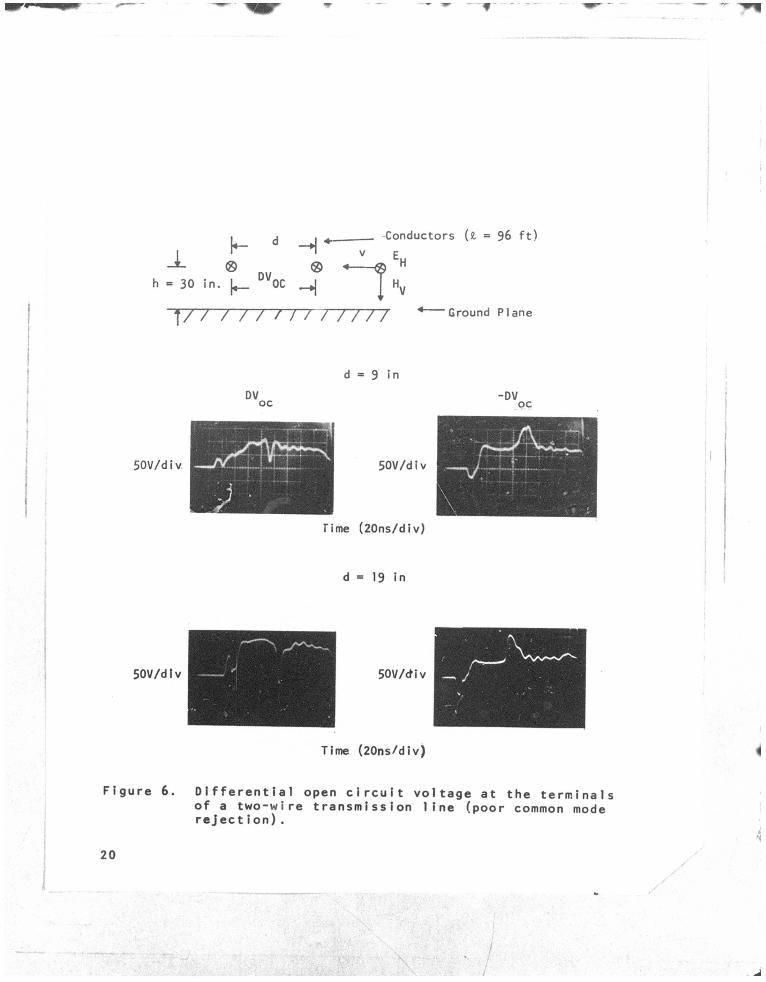
4.2.3 Di^ferential Voltage at ^he Terminals of a Two-Wire 'ransmission Line

Figure 5 shows the response for the differential voltage at th«; terminals of a two-wire transmission line. The computations for th. response were made using eq (9) with a = 0. To illustrate some problems which may be encountered when using a differential voltage probe, figure 6 shows a partly erroneous differential voltage measurement. (See section 5 for a discussion of this problem.)

4.2.4 Differential Current at the Terminals of a Two-Wire Transmission Line

Figure 7 shows the short circuit current at the terminals of a two-wire transmission line. The computations wtre made using eq (8) with a = 0.

5. CONCLUSIONS

5.1 Evaluation of the Description o? the Incident Field

The computation of the net electric field as discussed in section 2 is based on information about the electric free field radiated from the Bicone. This information can be extracted from measurements of EH and H . The validity of this approach has been supported by com- paring computations with experimental data: (1) The computed horizontal electric field at different heights above ground agreed well with measurements. (2) Calculations of currents and voltages on conductors with the computed field for the driving source compared well with measurements.

5.2 Evaluation of Transmission Line Theory for Computations of Current and Voltage Responses

The good agreement between computations and measurements support the analytical approach described in section 2, For the geompcries considered, the horizontal electric field component can be viewed as the major driving field for the coupling problem.

Errors can be introduced in the computation of the response of conductors close to the ground plane. These errors arise primarily as a result of difficulties in accurately.computing the incident field close to ground. Some of these difficulties can be removed by accurately determining the radiated free field (section 6) .

5.3 Instrumentation Problems

Sometimes it may happen that the instrumentation used for measur- ing the responses will record an incorrect result. It may be difficult to recognize such an error unless one knows what kind of response is expected. This is one of the reasons why an understanding of the coupling problem is important.

An example of the type of problem which may be encountered is shown in figure 6 . This figure shows the measured differential voltage for two different separations of the transmission line. Com- putations show that the result should be such as shown in figure 5 with the two measurements differing in amplitude only. The data in figure 6 clearly shows a common mode signal superiraposed on the differential signal, indicating a problem with the DV probe. (The measurement shown in figure 5 was made with a second DV probe.)

18

b h - 30 in . D»0(.

H ®

H

Conductors (2. = 96 f t )

v E •4——® '•

\> t / / / ' / / / / / / t / / / / Ground Plane

DV 50V 'd iv oc

20ns/d iv

d = 19 in

. 3 1 4—f~f 50V/div

j V / r *'

Time !>0ns/d i v

DV oc


Vol ts

800 --

0 200 400

Time (ns)


Figure 5• Differential open circuit vultage at the terminals of a two-wire transmission line.

19

\ I

_L ^ j ^ 4 Conductors (il = 96 f t )

v E ® ® •* H

DV h = 30 in . |^_ OC | H

\ / / / / / / / / / / / / / Ground Plane

50V/div 50V/div

Time (20ns/div)

d = 19 in

50V/dlv 50V/cfiv

Time (20ns/d iv )

Figure 6. Differential open circuit voltage at the terminals of a two-wire transmission line (poor common mode reject ion) .

20

d = 19 • n-J

30 in

Conductors (l = 36 f t )

v _ E.

•Ground Plane

'sc -2a/div

20ns/div

.2a/d i v

Time


50ns/div

SC

Amperes

200 kOO

Time (ns)


Figure 7• Short circuit differential current response at the terminals of a two-wire transmission line.

21

6 ■ RECOMMENDATIONS

6.1 Improved Computations of the Radiated Field

Accurate information about, the radiated froe field from the Bi- conc is required to correlate the Biconic free field to another field, such as the threat field for example. It can also be used for computing the net field at any point by applying the methods described in section 2. Better estimates of the radiated free field could be made by moaouring the requited !•; and H components at several points, computing the froe field and averaging the results.

6.2 Additional Studies of the Coupling Problem

The work described here considered the coupling problem for the case of an infinite conductivity ground plane only. In a practical situation, cables will be positioned above a finite conductivity ground plane. Hence, it is important to address this problem.

Obviously, the analytical work required is much more extensive in the latter case than in the former case. Sunde (ref. 3) has out- lined approximate solutions for the finite conductivity case. His basic approach is to compute modifications to the propagation constant and to the characteristic impedance, and apply the modified parameters to the usual transmission line equations. A comparison of theory and experiment would permit a useful evaluation of Sunde's approximate solutions.

22

GLOSSARY OF TERMS

.] R.icilus of Conductor L Inductance

C Ccipacilance R Distance from Center of Biccnic to Test Point

d Perpendicular Distance Between Two Wires R. Reflection Coerficient at

SC

Probe End Differential Short Circuit Current R- Reflection Coefficient at

End Away From Probe OV Differential Open Circuit

Voltage R,- Earth Reflection Coefficient E for Horizontal Electric Field

E Net Horizontal Electric Componem Field Component

Time Delay for Propagation Between Two Wires !

Component of the Free Field Distance, d, Apart E.L, Horizontal Electric Field Between Two Wires Spaced a UH

E Vertical Electric Field v Velocity of Propagation Component

g Ground Conductivity V.« Open Circuit Voltage

V(x) Voltage Distribution on h Height of Conductor Above Conductor Above Ground

Ground Y Transverse Admittance Per

h' Height of Biconic Above Ground Unit Length Along a Two Vi re Transmission Line

H Radial Magnetic Field Component Z Impedance Per Unit Length

H Vertica" Magnetic Field Along a Two Wire Transmission Component Line

I(x) Current Distribution on Z, Impedance at Probe End Conductor Above Ground

I

Z- Impedance at End Away from J(x) Transverse Current Distribution Probe

Between the Two Conductors of a Transmission Line Z Characteristic Impedance

a Attenuation Constant

r Propagation Constant

A Angle of Incidence

e Relative Dielectric Constant

Wave Length

Radial Frequency

r

23

APPENDIX A. Voltage and Current Response of a Two-Wi e Transmission Line (Broodside 111 umi nati on")

Broadside illumination refero to the condition in which the velocity vector of the incident electromagnetic field is perpendicular to the transmission line. The general solution to this problem is discussed in many textbooks. The discussion presented here follows the approach described by Sunde.'

Consider a short segment of a transmission line as shown in figure A-l. The voltage, V(x), is the voltage of line 2 at a point x with respect to line 1 at that point. The current, 1(x), at the point x, is equal in magnitude on both lines but opposite in direction. The basic differential equations for current and voltage along the trans- mifision line are:

1! dx ZL = -YV

and dV dx

= -Zl

(A-l)

(A-2)

A general solution for current and voltage mwjt be considered for two different cases.

CASE I - Incident Electric Field Vector Parallel to the Trans- mission Line

One obtains the solution to this problem by computing the response to the incident field on each line separately and using super- position to get the total response. If an electric field distribution, E (x) , is incident in the x direction along line 2, eq (A-2) must be modified to include E^x) as a source term. With this modification, and combining cq (A-ly and (A-2) we obtain:

d2l

dx -YEH(x) (A-3)

V(x)

Kx)

- I

dx

dl

V(x-t-dx)

(x+dx)

Figure A-l. Transmission line parameters,

1E. D. Sunde, Ea-th Conduction Effects in Transmission Systems, Dover Publications, Inc., New York (1967).

Preceding page blank

25

where r is the propagation constant

r = ^Yf

The general solution to eq (A-3) may be written as:

l(x) = [A < P{x)]e"rx -[B + Q(x)]erx

{A-4)

(A-5)

V(x) = Z FA + P(x)]e'rx + Z [B + Q(x)]erx

r o (A-6)

where

P(x) = ^L- f EuMervdV o Jo

(A-7)

Q(x) JT f EH(v

o Jo )e dv (A-8)

z = /Z7Y o

(A-9*

The constants A and B are detem ined by the boundary conditions at the ends of the conductors.

Consider the case when the transmission line is terminated by impedances Zi and Z2 at x = 0 and x = I, respectively. Applying the boundary conditions:

V(0) - =1(0)2 (A-10)

and

vU) - KOz, (A-ll)

We obtain;

B = R2PU)e'2rl-QU)

l-RjRje ■in (A-12)

A - BR, (A-13)

26

where Ri and R2 are the reflection coefficients at the terminations:

(A-14) R Zi-Z

1 o Z,+Z

1 o

Z9-Z _2 o Z„+Z 2 o

(A-15)

If the electric field vector is constant (in space) along line 2 then eq {A-7) and {A-8) are easily evaluated. Substituting for A, B, P, and Q in eq (A-5) and (A-6) we obtain:

l(x) _E_ ^ 2-(l+R))e-rx.(l+R2)e-I,(»-x)+RI(l+R2)e-r(£+x3

+R2(l+R1)e-r{2e-x)-2RIR2e-2ri ) /(l-R^.e"2")

and

(A-16)

V(x) = -5f^-{l+R))e-rx+(l+R2)e-r('-x)

+R](UR2)e-rU+x)

-R2(1+R])e •r(2«,-x) 1 /\\^R2e'2Vi)

(A-17)

The above solutions for the response have been derived for the field incident along line 2 only. For the total soultion, one must combine the solutions for the field incident on each line. The total solution will then be given by equations (A-16) and (A-17) , where the driving field EH is the difference in the fields incident on the two lines. Obviously/ a maximum response results when the field prop- agates in the plane of the two lines.

For a single conductor parallel to 1 ground plane of infinite conductivity, the modes of propagation f jr current and voltage along the conductor will be the same as those on a two-wire transmission line defined by the conductor and its image in the ground p]ane. Equations (A-16) (A-17) can be applied to the case of a single conductor parallel to ground by using the following modifications:

(1) The electric field incident on the conductor is the net electric field after reflection from the ground plane,

(;:) The characteristic impedance, Zo, is the characteristic imoedance of the conductor above the ground plane, and

(3) Equations (A-16) and (A-17) are divided by a factor of two.

27

CASE II - Incident Electric Field Vector Perpendicular to the Transmission Line

If an electric field distribution, E (x) , is incident with the electric field vector perpendicular to the transmission line, equation (A-l) must be modified to include E (x) as a source term. With this modification, and combining eg (A-lJ and (A-2) we obtain:

2 d V 2 —5- - r v = dx

-ZJ(x), (A-18)

where J (x) is the current source density for a spacing, d, between the conductors and an electric field, Ev (x) , in the plane of the conductors :

J(x) = Ev(x)dY {A-19)

The solution to Equation (B-18) may be written as:

l(x) = [A+P(x)]e"rx -[B-Q(x)]erx {A-20)

V(x) = Zo[A+P(x)]e"rx fZo[B-Q(x)]erx (A-21)

where

P(x) = i r"jMerVdv

a(x) - j r"jMe'rvdv.

(A-22)

(A-23)

The constant A and B are determined by the boundary conditions at the ends of the conductors. Consider the case when the transmission line is terminated by impedances Zi and Z2 at x = 0 and x = «,, respectively. Applying the boundary conditions, equations (A-IO) and (A-ll) we obtain:

B - R2PU)e'2rVQU)

l-R^e •2n (A-24)

BR.

28

If the electric field vector is constant (in space) along the transmission line then eq (A-22) and (A-23) are easily evaluated. Substi- tuting for A, B, P and Q in eq (A-20) and (A-21) we obtain:

w .v_ { .(I.Ve-rx+(1.Rpe-rU-x) .R](1.R2)e-rU+x) 2Z

(A-25)

^(l-Rê-^2^' ) /(I-R^^-2")

and

VW = !f I 2-(l-R|)e-rx-(l-R2)e-rU-x) -R^l-Rê-^^

-R^l-Rê"^2^ 2R1R2e-2rA /(1-R, ê"2^) (A-26)

The solutions derived for the two cases (incident electric field vector parallel and perpendicular to the transmission line) have been staued as single frequency solutions. Fourier analysis or Laplace transform techniques must be used to obtain the solutions for the general case of a transient incident field.

29

distributed by: national technical information service u ... · werner j, stark harry diamond...

Documents