do peer group members outperform ... - bank of canada

Bank of Canada Banque du Canada

Working Paper 2003-33 / Document de travail 2003-33

Do Peer Group Members OutperformIndividual Borrowers? A Test of Peer GroupLending Using Canadian Micro-Credit Data

by

Rafael Gomez and Eric Santor

ISSN 1192-5434

Printed in Canada on recycled paper

Bank of Canada Working Paper 2003-33

October 2003

Do Peer Group Members OutperformIndividual Borrowers? A Test of Peer GroupLending Using Canadian Micro-Credit Data

by

Rafael Gomez 1 and Eric Santor 2

1London School of EconomicsLondon, England WC2A 2AE

2International DepartmentBank of Canada

Ottawa, Ontario, Canada K1A [email protected]

The views expressed in this paper are those of the authors.No responsibility for them should be attributed to the Bank of Canada.

iii

Contents

Acknowledgements. . . . . . . . . . . . . . . . . . . . . . . . . . . . . . . . . . . . . . . . . . . . . . . . . . . . . . . . . . . . ivAbstract/Résumé. . . . . . . . . . . . . . . . . . . . . . . . . . . . . . . . . . . . . . . . . . . . . . . . . . . . . . . . . . . . . . . v

1. Introduction . . . . . . . . . . . . . . . . . . . . . . . . . . . . . . . . . . . . . . . . . . . . . . . . . . . . . . . . . . . . . . 1

2. Why Should Peer Group Members Outperform Individual Borrowers?. . . . . . . . . . . . . . . . 2

2.1 Previous empirical literature. . . . . . . . . . . . . . . . . . . . . . . . . . . . . . . . . . . . . . . . . . . . . 3

3. The Data. . . . . . . . . . . . . . . . . . . . . . . . . . . . . . . . . . . . . . . . . . . . . . . . . . . . . . . . . . . . . . . . . 3

3.1 Sample considerations . . . . . . . . . . . . . . . . . . . . . . . . . . . . . . . . . . . . . . . . . . . . . . . . . 3

3.2 Sample characteristics. . . . . . . . . . . . . . . . . . . . . . . . . . . . . . . . . . . . . . . . . . . . . . . . . . 4

3.3 Statistics on default rates and loan terms . . . . . . . . . . . . . . . . . . . . . . . . . . . . . . . . . . . 5

3.4 Demographic, household, and business characteristics of borrowers. . . . . . . . . . . . . . 5

3.5 Group versus individual borrowers. . . . . . . . . . . . . . . . . . . . . . . . . . . . . . . . . . . . . . . . 7

3.6 Delinquent versus successful borrowers. . . . . . . . . . . . . . . . . . . . . . . . . . . . . . . . . . . . 7

4. Empirical Specifications . . . . . . . . . . . . . . . . . . . . . . . . . . . . . . . . . . . . . . . . . . . . . . . . . . . . 8

4.1 The standard regression estimation. . . . . . . . . . . . . . . . . . . . . . . . . . . . . . . . . . . . . . . . 8

4.2 Isolating the incentive effects of peer group lending . . . . . . . . . . . . . . . . . . . . . . . . . . 9

5. Results . . . . . . . . . . . . . . . . . . . . . . . . . . . . . . . . . . . . . . . . . . . . . . . . . . . . . . . . . . . . . . . . . 13

5.1 Does belonging to a peer group reduce borrower default? . . . . . . . . . . . . . . . . . . . . . 13

5.2 Does belonging to a peer group reduce the size of borrower default? . . . . . . . . . . . . 14

5.3 Accounting for self-selection . . . . . . . . . . . . . . . . . . . . . . . . . . . . . . . . . . . . . . . . . . . 15

5.4 Robustness check I: comparing probit results across peer loan subgroups . . . . . . . . 16

5.5 Robustness check II: comparing matching with “fine” and “coarse”. . . . . . . . . . . . . 17

6. Conclusion . . . . . . . . . . . . . . . . . . . . . . . . . . . . . . . . . . . . . . . . . . . . . . . . . . . . . . . . . . . . . . 18

Bibliography . . . . . . . . . . . . . . . . . . . . . . . . . . . . . . . . . . . . . . . . . . . . . . . . . . . . . . . . . . . . . . . . . 19

Tables . . . . . . . . . . . . . . . . . . . . . . . . . . . . . . . . . . . . . . . . . . . . . . . . . . . . . . . . . . . . . . . . . . . . . . 22

Figures. . . . . . . . . . . . . . . . . . . . . . . . . . . . . . . . . . . . . . . . . . . . . . . . . . . . . . . . . . . . . . . . . . . . . . 44

Appendix A: A Note on Calmeadow’s Lending Mechanism . . . . . . . . . . . . . . . . . . . . . . . . . . . . 48

iv

Acknowledgements

We would like to thank Dwayne Benjamin, Albert Berry, Jon Cohen, Martin Connell, David De Meza,

Morley Gunderson, Sonia Laszlo, Kevin Milligan, Jim Pesando, Konstantinos Tzioumis, and the

staff of Calmeadow Metrofund and Calmeadow Nova Scotia for assistance and helpful comments.

Financial support was provided by the Social Science and Humanities Research Council and the

Canadian Employment Research Forum.

v

eer

g

wer

h the

ater

ages

de partie

t très

ontrent

ins

opérée

Abstract

Microfinance institutions now serve over 10 million poor households in the developing and

developed world, and much of their success has been attributed to their innovative use of p

group lending. There is very little empirical evidence, however, to suggest that group lendin

schemes offer a superior institutional design over lending programs that serve individual

borrowers. The authors find empirical evidence that group lending does indeed lower borro

default rates more than conventional individual lending, and that this effect operates throug

dual channels of selection into the peer lending program and, once inside the program, gre

group borrower effort.

JEL classification: J23, O17, E82Bank classification: Development economics

Résumé

Les institutions de microfinance prêtent aujourd’hui des fonds à plus de 10 millions de mén

pauvres dans les pays en développement et les pays développés. Leur succès est en gran

attribué au fait qu’elles recourent à une forme originale de prêt collectif. Il existe cependan

peu d’éléments empiriques attestant que ces mécanismes soient mieux conçus que les

programmes de prêt aux particuliers. Les auteurs obtiennent des résultats empiriques qui m

que les participants aux programmes de prêt collectif présentent un taux de défaillance mo

élevé que les emprunteurs individuels, et que ce phénomène est dû à la fois à la sélection

au départ et aux efforts accrus que les membres d’un groupe d’emprunteurs déploient.

Classification JEL : J23, O17, E82Classification de la Banque : Économie du développement

1

e of

ners

stock

ists

mics

ual

effort

stions

n

mes

onfirm

n but

of

e

ties.

side

re are

with

es not

ting)

laims

nal

how

al

st

1. Introduction

Microfinance institutions (MFIs) now serve over 10 million households worldwide and are

expanding throughout the developing and developed world.1 Despite the relative poverty of their

clients, MFIs have been able to extend credit to poor households through the innovative us

group lending, while maintaining high repayment rates and financial sustainability. Practitio

and pundits attest to the ability of group lending to increase incomes, consumption, and the

of human capital of households that lack collateral and face severe credit constraints. Not

surprisingly, the apparent success of peer group lending has drawn the attention of econom

from both theoretical and applied perspectives.

This paper addresses two empirical questions that remain largely unanswered in the econo

literature: (i) does peer group lending lead to higher repayment rates than traditional individ

lending techniques, and (ii) is the beneficial peer group effect the result of greater borrower

or the consequence of positive self-selection into the group lending program? These two que

lie at the heart of the microfinance debate and therefore warrant close empirical scrutiny. A

affirmative answer to the first question, for example, would explain why group lending sche

are instituted in the first place, whereas a positive response to the second question would c

theoretical and practitioner claims that peer groups not only perform a useful sorting functio

provide positive spillovers to all those enrolled in such programs, by inducing higher levels

borrower effort.

Utilizing data from two North American microfinance institutions, we find evidence that thos

enrolled in group loan programs outperform individual borrowers in terms of default probabili

We attribute this effect to the dual channels of sorting and incentives for greater effort once in

the group. Employing both self-selection and matching methods estimates, we find that the

unobserved characteristics that lower the likelihood of default, and that they are correlated

being in a peer group program. However, this positive selection into a peer group program—

though it reduces the magnitude of the peer loan probit results by roughly 20 per cent—do

eliminate the significance of the peer group effect, which indicates that greater effort (not sor

is the dominant channel by which group lending improves borrower performance.

This paper is organized as follows. Section 2 outlines the central theoretical and empirical c

and reviews the relevant literature that shows that peer group lending is a superior institutio

mechanism compared with conventional individual lending techniques. Section 3 describes

the data were collected and presents descriptive statistics. Section 4 describes the empiric

1. The Grameen Bank in Bangladesh, BancoSol in Bolivia, and Bank Raykat Indonesia are the mocommonly cited examples of MFIs. See Morduch (1999) for a brief review of these institutions.

2

nd

works

es can

ts.

igate

es.

each

idual

how

ure

99).

levels

that

f such

owers

e

, van

),

e

me.at

methodology used. Section 5 provides the empirical results. Section 6 offers conclusions a

identifies areas of further research.

2. Why Should Peer Group Members Outperform IndividualBorrowers?

In recent years, considerable effort has been made to understand both how group lending

and the effect it may have in practice. Most studies have focused on how peer group schem

overcome the inherent problems associated with asymmetric information in financial marke2

Specifically, in a world where borrowers lack collateral, group lending has been shown to mit

problems associated with adverse selection, moral hazard, contract enforcement, and state

verification (Morduch 1999; Ghatak and Guinnane 1999). Group lending with joint liability

overcomes these problems by passing the monitoring activity on to the borrowers themselv

The idea is that group members will monitor their peers and pressure those individuals who

misuse their loans to act accordingly.3 While this monitoring activity is costly for the borrower, it

is assumed to be much less so than for the lender, since group members will typically know

other well in advance of the date of borrowing.4 Assuming that monitoring costs are low and

social sanctions effective, Ghatak and Guinnane (1999) show that, compared with an indiv

liability contract, effort will be strictly higher under joint liability.5 The implications of these

findings also agree with the results reported in the personnel economics literature, which s

that team-based production can have both sorting and incentive effects and that peer press

within a team can have a discernible impact on worker effort and individual output (Lazear 19

Theoretical models, therefore, demonstrate that peer group schemes tend to induce higher

of effort by borrowers due to intrapersonal monitoring and peer pressure. Although it is true

closer monitoring and increased effort is inherently difficult to measure, the consequences o

peer group effects are easier to observe: group members should outperform individual borr

in terms of repayment success (holding all else constant).6 We seek to measure this basic outcom

2. See, for example, Ghatak (2000), Laffont and N’Guessan (2000), Ghatak and Guinnane (1999)Tassel (1999), Armendariz de Aghion and Gollier (1998), Stiglitz (1990), and Varian (1990).

3. The theoretical models of Stiglitz (1990), Varian (1990), Banerjee, Besley, and Guinnane (1994Conning (2000), and Armendariz de Aghion (1999) draw heavily on this concept.

4. The cost of monitoring for group members should be relatively low if one accepts that assortativmatching occurs.

5. The effectiveness of peer group lending depends heavily on the notion that there is a long-runrelationship between borrowers. If borrowers do not have a close relationship to their fellowborrowers, social sanctions would not be effective. In this sense, group lending is a repeated ga

6. Joint liability is not the only operative feature of group lending; there may be other mechanismswork, such as risk pooling, spillover effects, and the ability of lenders to lower transaction costs.Likewise, many MFIs employ other innovative lending techniques that can improve repaymentperformance, such as more timely repayment schedules and dynamic incentives.

3

ages

with

p

ir

l ties,

up

of

of

ing

the

ort.

uld

e

idual

ce ofnder.

er

mized

and, if possible, to distinguish the incentive effects of group lending from any of the advant

brought about by sorting and self-selection into the peer group program.

2.1 Previous empirical literature

Despite the strong predictions of group lending models, there is little or no direct empirical

evidence to suggest that peer group members actually outperform individual borrowers.7 For

instance, Ahlin and Townsend (2003) test a wide range of the predictions of group lending

joint liability, such as the impact of interest rates, loan size, the degree of joint liability, grou

homogeneity, and the level of group monitoring and social sanctions. Although much of the

evidence confirms the predictions of theory, they find evidence that proxies for strong socia

group monitoring, and group co-operation are negatively related to repayment.8 On the other

hand, Karlan (2003) shows that higher levels of social capital are positively correlated with

repayment, particularly when facilitated by the appropriate environment. Wydick (1999a)

suggests that groups matter, in that greater levels of social cohesion (such as knowing gro

members prior to group formation or living in the same neighbourhood) lead to lower levels

individual default. Wenner (1995) offers similar evidence that socially cohesive groups have

higher repayment rates. Although many of the key predictions of group lending have been

confirmed, no published study has yet compared individual borrower outcomes with those

comparable group members. Therefore, despite growing empirical evidence, two principal

theoretical conjectures concerning peer groups remain unanswered: (i) whether group lend

leads to lower default rates than individual lending techniques, and (ii) whether this effect is

result of positive selection into the peer group program or the result of greater borrower eff

3. The Data

3.1 Sample considerations

The effectiveness of group lending, as predicted by the theoretical models noted earlier, wo

ideally be tested using a randomized experiment.9 That is, to avoid problems of self-selection, on

would like to run an experiment where borrowers are randomly placed into group and indiv

7. Ghatak and Guinnane (1999) note that “there is little empirical evidence on the relative importanjoint liability as opposed to other program features,” such as direct monitoring on the part of the le

8. Ahlin and Townsend (2003) find that lower interest rates, lower joint liability payments, and highlevels of human capital are correlated to higher repayment rates.

9. See Heckman and Smith (1996) for a discussion of the advantages and disadvantages of randoexperiments in assessing program effectiveness.

4

ce are

e must

ng

n

tics.

d

n

vides

nt

hold,

t the

ion

-

’soes atate its

lyake it

oanal

as a

loan programs and the respective treatment and control group’s loan-repayment performan

assessed. To date, MFIs have been unwilling to conduct such experiments and therefore on

resort to non-experimental regression techniques.

Not surprisingly, non-experimental techniques require rich data to test whether group lendi

with joint liability leads to higher repayment rates. The MFI from which data might be drawn

must possess the following three attributes: (i) provision of group and individual loans, (ii) a

accurate record of loan repayment, and (iii) a detailed profile of their borrower’s characteris

Very few MFIs, if any, offer both group and individual loans, collect sufficient client data, an

accurately assess the true rate of borrower default.10 This lack of data can be attributed to intrinsic

features of the microfinance world.11

Fortunately, the data collected for this study, which are drawn from two MFIs—Calmeadow

Metrofund (located in Toronto) and Calmeadow Nova Scotia (located in Halifax)—provide a

opportunity to test the predictions of the theoretical models discussed above. Calmeadow pro

data on both group and individual loans, maintains accurate records of client loan-repayme

performance and collects a wide range of client information, including demographic, house

and business characteristics.12 Appendix A provides a brief description of Calmeadow’s

institutional features, and highlights the advantages of the data.

3.2 Sample characteristics13

The data consist of 1,389 borrowers who accessed loans from Calmeadow Metrofund and

Calmeadow Nova Scotia. There are 995 group and 394 individual borrowers, who represen

entire population of Calmeadow clients from 1 January 1994 to 30 August 1999.14 For each

borrower, demographic, business, and household data are extracted from the loan applicat

contained in Calmeadow’s client file, and repayment history is gathered from the GMS loan

10. For instance, Morduch (1999) shows that the Grameen Bank, despite being one of microfinanceflagship programs, consistently underreports its default rates at the institutional level. It is easy timagine that local loan managers would have equally great incentives to underreport arrears ratthe individual or group level. For a detailed discussion as to why the Grameen Bank may understdefault rate, see Morduch (1999).

11. First, many MFIs lack the resources to collect such detailed data and, second, they may have onrudimentary accounting systems or alternative agendas (such as satisfying donors) that may mdifficult to obtain information on clients, repayment rates, and loan arrears.

12. Calmeadow transferred its micro-lending operation to the MetroCredit Union in January 2001. Lrepayment history is tracked through GMS, a software package designed specifically for financilending institutions.

13. All descriptive results are given in Tables 1 to 6.14. The majority of the borrowers in the sample accesssed their loans from 1996 to 1999 and this w

period of considerable macroeconomic stability in the Metropolitan Toronto and Halifax areas.

5

the

es

and

ow’s

ers,

per

up

NSF

he

ards,

an

, with

for

al

per

th for

d for

e of

ronto

nts,

cy, oreend of

ority.iontics.

tracking system. The data have been supplemented by a telephone survey (conducted by

authors in July 1998 and available from them upon request) that measured borrower attitud

towards repayment and other normally hard-to-observe characteristics, such as the nature

abundance of social ties. The following subsections provide descriptive statistics of Calmead

clients, placing particular emphasis on the differences between group and individual borrow

and successful and delinquent borrowers.

3.3 Statistics on default rates and loan terms

The default rate for Calmeadow borrowers is fairly high by microfinance standards, but not

outrageously so.15 The data reveal that roughly 21.2 per cent of all group borrowers and 41.4

cent of all individual borrowers have defaulted on their loans. Likewise, 38.4 per cent of gro

borrowers and 88.7 per cent of individual borrowers have an “NSF” recorded on their loan (

implies a missed payment). In terms of the ratio of write-offs to outstanding loan portfolio, t

arrears rate is approximately 8 per cent. While seemingly high by conventional banking stand

the arrears rate at Calmeadow is similar to the average rate reported by most North Americ

MFIs.

Group loans range from $500 to $5,000 and individual loans range from $1,000 to $15,000

mean and median loan sizes of $1,031 and $1,000 for group loans and $3,954 and $2,700

individual loans, respectively. Loan terms vary from 6 to 24 months for group loans; individu

loans offer longer terms to a maximum of 60 months. The cost of both types of loans is 12

cent plus an up-front administration fee of 6.5 per cent. Loan payments average $95 per mon

group borrowers and $220 per month for individual borrowers. Group loans are typically use

working capital, while individual loans are often used for working capital and/or the purchas

fixed assets.

3.4 Demographic, household, and business characteristics of borrowers

Calmeadow’s clients are demographically diverse and representative of the population of To

and Halifax.16 Approximately 52 per cent of all clients are female and 39 per cent are immigra

15. For this study, default is defined as any loan that has been “written off,” sent to a collection agenis “non-performing.” Non-performance includes any loan where three or more payments have bmissed. The definition of default used in this study conforms to the commercial banking standar“non-performance” and provides a reasonably accurate picture of repayment performance.

16. The notable difference between the Toronto and Halifax borrowers is that Halifax clients arepredominantly native-born Caucasians, with a significant Canadian-born African-Canadian minOnly 10 per cent of Halifax borrowers are immigrants. Apart from differences in ethnic compositand immigrant status, the two groups are virtually the same across most observable characteris

6

mple is

n

s

hool

alf of

side

jority

arily

f the

edian

t

or

tions

written

it (or

onthly

edian

t

of

s of

ast

ups

age of

sonal,

items

elopedurce

ies

51 per cent are white, and most major ethnic groups are present (Tables 2a and 2b). The sa

more heavily weighted in favour of African-Canadians, however, and East- and South-Asia

Canadians are underrepresented.17 The average borrower is 43 years old, with two dependant

and more education than the general population (over 52 per cent have post-secondary sc

diplomas or degrees). The majority of Calmeadow Metrofund’s borrowers live in the city of

Toronto, and its remaining clients are dispersed across the Metropolitan region. Likewise, h

all Calmeadow’s Nova Scotia clients live in the Halifax-Dartmouth area, and the remainder re

in various small communities scattered across Nova Scotia.

Table 3 highlights the extent to which Calmeadow serves credit-constrained clients. The ma

of clients, while obviously credit constrained, nevertheless have other sources of credit (prim

in the form of credit cards). However, 39 per cent rely solely on Calmeadow for their funds. O

86 per cent of clients who have a credit history, the median credit limit is $2,722 and the m

net limit (credit limit less outstanding balance) is only $62. Consequently, the median credi

utilization rate is 98 per cent. Likewise, significant portions of Calmeadow clients have a po

credit history: 10 per cent have previously declared bankruptcy, 13 per cent have debt obliga

sent to a collection agency, and 40 per cent have had at least one “R9,” a debt that has been

off by the credit grantor. Overall, roughly 46 per cent of all borrowers have “bad credit.”

Consequently, one can assume that Calmeadow is serving clients who cannot access cred

further credit) from conventional sources.

The household characteristics reveal that the average Calmeadow client is poor. Average m

non-business household income is $1,510 (median $1,200) and net worth is only $10,930 (m

$4,620) (Table 4).18 Many clients (49 per cent) have a wage or salary income and 27 per cen

receive some kind of government assistance. Roughly half of all clients do not work in paid

employment, and 40 per cent cite self-employment income as their “major” or “only” source

income.

The average business operated by a Calmeadow client is very small, with monthly revenue

only $3,239 (median $1,700) and monthly profits of $1,110 (median $600) (Table 5). The v

majority of clients run sole proprietorships located in their home, over 37 per cent are start-

(less than one year in operation), and existing businesses have been operating for an aver

two years. The businesses cover a wide range of activity, but most provide some form of per

business, or retail service. A small but significant minority of businesses manufacture small

17. This may represent the fact that South- and East-Asian Canadians (in particular) have well-devinformal credit markets within their ethnic community and thus Calmeadow is not an attractive soof credit.

18. This figure is likely biased upwards significantly. Anecdotal evidence suggests that, while liabilitare well reported (due to their verification), assets are systematically overestimated.

7

es.

roup

al

tivity.

ssets

to

have

ared

re

those

larger

owers.

ess

e,

tside

are

s,

who

feel

to

(artisanry or jewelry manufacturing, for example) or own construction/landscaping business

Apart from this last category, most businesses are similar in size and composition.

3.5 Group versus individual borrowers

There are several key demographic differences between group and individual borrowers. G

borrowers are more likely to be female, of Hispanic ethnicity, and immigrants, while individu

borrowers are more likely to be of African ethnicity, male, and born in Canada (Table 2a).

Individual borrowers have less education but more skills training related to their business ac

With respect to household characteristics, individual borrowers have higher incomes and a

but similar net worth, rely more heavily on their self-employment income, and are less likely

receive government assistance. Although there are still many start-ups, individual borrowers

larger and older microenterprises than group borrowers (monthly revenues of $5,889 comp

with $2,579) and higher profit levels. Likewise, individual borrowers run proportionately mo

storefront locations and are more likely to be incorporated.

3.6 Delinquent versus successful borrowers

There are significant differences between borrowers who successfully repay their loans and

who fail to fulfill their obligations to Calmeadow Metrofund. In terms of loan terms and size,

delinquent borrowers tend to have, at the mean, slightly larger loans, with longer terms and

monthly payments. The ratio of household income to loan payment is higher for successful

borrowers, but business revenues and profits to loan payment are higher for delinquent borr

Demographically, delinquent borrowers tend to be single, male, and born in Canada, with l

education and significantly lower levels of business-related skills training. Household incom

assets, and net worth are slightly lower, but statistically similar. Delinquent borrowers lack ou

sources of credit: for those who do have credit, their “credit utilization” rate is higher and they

more likely to have a poor credit history. In terms of business type, there are only a few

differences in terms of activity, revenues, profits, and ownership type. Delinquent businesse

however, tend to be start-ups located outside the home.

Within the groups themselves, attitudinal differences appear in the survey data. Delinquent

borrowers are less likely to feel a moral obligation to repay their loans (Table 6). Individuals

have known their fellow members before forming the peer group are less likely to default.

Likewise, default is less likely if a great deal of trust exists in the group or if group members

a moral obligation to their peers. Lastly, individuals who have “social capital” are less likely

8

iness

repay.

cate

hic,

d

on the

e,

hold,

hat

, the

he

ored

default, since individuals who belong to an association, club, or sports team report higher

repayment rates.19

4. Empirical Specifications

4.1 The standard regression estimation

The descriptive statistics reveal that there are important demographic, household, and bus

differences between those borrowers who default on their loan and those who successfully

Utilizing this information (and one can imagine that loan managers do so less formally to allo

loans), one can form a prediction regarding the likelihood of default based upon demograp

household, and business characteristics. This credit-scoring approach can follow several

functional forms, including linear discriminant analysis, logit/probit regression, or, as applie

more recently, neural net learning techniques. In practice, credit scoring has relied heavily

first two methods, with a bias towards utilizing logit/probit techniques (Thomas 2000).

More specifically, a credit-scoring model20 that could be used to assess the effect of group

membership would first propose that there is an index function with a latent regression,

, (1)

where the dependent variable, , is the propensity to default andi indexes over the individual.

The likelihood of default is a function ofXi, a set of borrower characteristics that includes incom

home ownership status, employment records, and credit history; other demographic, house

and business, and neighbourhood and institutional characteristics; and a dummy variable t

indicates peer group membership.21 The probability of default can thus be expressed as

.

Given that has the standard properties (normally distributed with mean 0 and variance 1)

default probability is,

, (2)

19. For a discussion of the effects of social capital, as measured by membership in civil society, on tperformance of microfinance borrowers, see Gomez and Santor (2001).

20. This section follows Greene (1998).21. Institutional-level characteristics include which MFI manager screened the applicant and monit

the loan.

Di* βXi εi+=

D*

Pi Prob Di 1 Xi=[ ]˙=

ε

Prob Di 1 Xi=[ ] Φ βXi( )=

9

ate

rd

is

spect

ere the

her

the

Tobit

n

al and

ative

not so

we

e

the

r and

where is the standard normal cumulative distribution function. This allows one to estim

the following probit model:

, (3)

where is a discrete binomial variable ( indicates that the borrower defaults, 0

otherwise), and the subscripti indexes over the individual whileg indexes over the group. The

matrix of borrower characteristics,X, group level characteristics, and a dummy variable,G,

indicate that the borrower is a member of a peer group. The error term, , has the standa

properties. The key prediction of group lending with joint liability can be assessed within th

regression framework. That is, do group borrowers outperform individual borrowers with re

to loan repayment?

A second specification based on a standard regression framework can also be utilized, wh

dependent variable is the amount of the loan written off, . This is done to examine whet

group lending mitigates not only the likelihood of default, but also the severity of default.

Therefore, we also estimate the following Tobit model,

, (4)

, (5)

where is a latent variable that is a continuous measure of the loan write-off,X is the matrix of

borrower characteristics that is equivalent to the specification in (3), and the error term has

standard properties. Since is truncated at zero for borrowers that successfully repay, the

specification is warranted.

The hypothesis that group borrowers should outperform individual borrowers in terms of loa

repayment can be tested by estimating models (3) and (4) for the entire sample of individu

group borrowers. If peer groups induce higher levels of borrower effort, then should be neg

and significant in both cases. Unfortunately, the empirical procedures described above are

straightforward, as self-selection into the peer group program needs to be accounted for if

wish to identify whether the incentive effects of group lending are operative.

4.2 Isolating the incentive effects of peer group lending

A useful way of isolating the incentive channels in models (3) and (4) is to consider as th

“treatment” effect of belonging to a peer group, while being an individual borrower indicates

absence of the treatment. If program participation is exogenous, then the decision to apply fo

Φ( )•

Dig α βXig θGig εig+ + +=

Dig Dig 1=

εig

Lig

Yig* α βXig θGig εig+ + +=

Yig*

0 if Yig 0 Yig if Yig 0>;≤{ }=

Yig

Yig

θ̂

θ

10

vide

g

rowers

ram.

ted

n the

ncome,

n-

ates of

gle

m.

rs. If

are not

atment

ble

receive a group loan is independent of the probability of default and the estimate of will pro

an unbiased measure of the treatment (incentive) effect. In the case of Calmeadow’s lendin

program, however, it is evident that participation is not exogenous, because only those bor

who have large projects and sufficient collateral are able to access the individual loan prog22

Consequently, one needs to determine how endogenous program participation will bias the

results, and how this bias can be accounted for in the estimation procedure.

4.2.1 Estimation of non-experimental treatment effects

To account for endogenous program participation, a treatment-effects model can be estima

following Greene (2000). In this framework, one estimates the average impact of program

participation as:

, (6)

where is the outcome if the treatment is taken up, and if not;G = 1 indicates that the

borrower is eligible to take up the treatment, andG = 0 otherwise.

Though useful, the non-experimental technique described above relies on the fact that the

treatment and control groups share common supports for the distribution of borrower

characteristics. However, if the supports of the distribution are not similar—i.e., borrowers i

treatment and control group are not comparable across a range of characteristics, such as i

education, or gender—Heckman et al. (1996) show that the implementation of standard no

experimental techniques may produce biased estimates of program impacts, because estim

program effects assume that the impact of the program can be captured entirely by the sin

index, ßX, which may not be related to the borrower’s propensity to participate in the progra

Furthermore, simple probit regression implies a common program effect across all borrowe

the treatment group responds differently to the treatment, however, then these differences

resolved by the standard treatment-effects model.

4.2.2 Why not a randomized experiment?

To accurately assess the impact of the program, one needs to calculate the effect of the tre

(the group lending program) on the treated (those who accessed the program):

. (7)

22. Unbiased estimates of can still be obtained if the sources of self-selection occur over observacharacteristics (Heckman and Hotz 1989; Heckman and Smith 1996).

θ

θ̂

θ E D1 | G = 1( ) E D0 | G = 0( )–=

D1 D0

θT E D1 | G = 1( ) ED0 | G = 1)–=

11

nd

he

and

(7)

ue that

cessed

ay be

ble to

ized

effects

e

d.

by

wer in

r the

and

biased

is that

ntify

n

g

That is, one needs to observe the outcomes of the borrowers that received the treatment a

compare them with a set of borrowers that are otherwise identical, except for the fact that t

control group did not have access to the program (but are eligible to take up the treatment

would do so, given its availability). Unfortunately, the second term of the right-hand side of

does not exist in the data, since it is not observed.

A solution is for the researcher to create by implementing a randomized

experiment: borrowers would apply to the group lending program and a proportion of those

accepted would be randomly denied access. This would create a true control group analog

could be used to determine the difference between the outcomes of those borrowers that ac

the program and the outcomes if the program had not existed. A randomized experiment,

however, may not generate useful counterfactuals in this case, since one of the underlying

mechanisms of group lending is endogenous group formation. While some group effects m

present in the randomized experiment, the underlying motivational factors that are attributa

social capital and assortative matching within the group would be omitted. Although random

experiments have been successfully implemented in the presence of endogenous selection

in certain settings, these approaches are not feasible here, since, as noted earlier, MFIs ar

unwilling to conduct such an experiment.23 Therefore, other approaches need to be considere

4.2.3 A matching-methods approach

In our case, a solution to this evaluation problem is to create the counterfactual

matching treatment and control borrowers along observable characteristics. For every borro

the treatment, one can find an individual borrower who is identical in every respect, except fo

availability of a group lending loan. Since there are many dimensions along which to match

borrowers, finding comparable matches in any conventional way becomes difficult if not

impossible.

Fortunately, there is a solution to this problem, known as “matching methods.” Rosenbaum

Rubin (1983) show that, instead of matching alongX, one can match alongP(X)—the probability

that the borrower participated in the treatment group—and thus estimate consistent and un

estimates of the effect of program participation on the treated. The advantages of matching

it exploits all the endogenous information on program participation, without the need to ide

program participation through functional form or excluded instruments (Ham, Li, and Reaga

2003).

23. A large literature has evolved around the use of randomized experiments to evaluate job traininprograms. See Heckman and Smith (1996) for a complete survey.

E D0 | G = 1( )

E D0 | G = 1( )

12

logue

data

come

d third,

able

is a

p may

the

nt

e

may

1).

ction

ment

or

se

siness

teria

ly

The ability of matching-method techniques to construct a suitable control-group sample ana

depends on the following crucial assumption:

. (8)

That is, conditional on the propensity score, the outcome in the non-participation state is

independent of participation. For this result to hold, Smith and Todd (2001) suggest that the

must possess the following criteria. First, the data for the control and treatment group must

from the same source; second, the outcomes must occur in the same geographic region; an

the data must be “sufficiently rich” that (8) holds. The limitations of matching methods are a

function of these conditions and, in particular, of the third criterion. The ability to create suit

counterfactuals to the treatment group depends on being able to match along observable

characteristics. If the process of selection into the participation and non-participation states

function of unobservables that are not captured by the observable data, then the control grou

not be properly specified (Ham, Li, and Reagan 2003). In this sense, the limitation of utilizing

propensity score as a measure of “comparability” is determined by the availability of sufficie

conditioning variables. If the decision to participate in the program is poorly measured, the

treatment and control groups will be poorly matched, and any inferences on the effect of th

“treatment on the treated” will be biased in an undetermined manner. In this way, matching

actually accentuate the biases caused by selection on unobservables (Smith and Todd 200

4.2.4 Is our data appropriate for a matching-methods approach?

Fortunately, the Calmeadow data are sufficiently rich that the sources of sorting and self-sele

that place borrowers into group and individual loans are easily observable, because the

requirements outlined in Calmeadow’s loan-application process formally determine the place

of borrowers (ex ante) into group or individual loans based on specific characteristics. For

instance, to qualify for an individual loan, the borrower must have a business one year old

older, provide a sophisticated business plan, have self-employment training, and pledge

collateral.24 These criteria imply that individual borrowers will have larger businesses, more

skills, and greater household resources than group borrowers. The data can control for the

differences between borrowers, because there is information available on start-up status, bu

size, and household resources (in terms of household income and net worth). While the cri

24. While the individual loan application states that collateral is necessary, this requirement is mostsymbolic. Typically, the security agreement utilizes the asset to be purchased as the collateral.Consequently, the collateral requirement is rarely, if ever, a barrier to accessing loans (this isreinforced by the fact that Calmeadow executed on a security agreement only once in the periodcovered by the sample).

E D( 0 P X( ) G, 1) E D( 0 P X( ) G, 0)= = =

13

e

ital,

iven

f

um

tive

tage

d

e peer

l

t risk)

ity to

many

Is.

eer

ing

nt. In

gers

rtain

p

our

than

atedo not

that places a borrower into an individual or group loan appears limited, there are other

characteristics that sort borrowers into the appropriate loan type. The requirement of a mor

sophisticated business plan indicates the need for differentially higher levels of human cap

while a longer loan term for individual borrowers suggests differential borrower-side risks. G

the extensive nature of the Calmeadow data, the potential biases stemming from the use o

matching methods are greatly mitigated in this instance.25

5. Results

5.1 Does belonging to a peer group reduce borrower default?

To answer this key question, Table 7 reports the results from estimating model (3) by maxim

likelihood. The effect of being in a group, when controlling for many typical variables, is nega

with respect to loan defaults in all specifications, columns 1 through 4. Measured in percen

terms (Table 7, column 1), we find that group lending reduces the probability of default by

roughly 17 per cent more than individual lending. When one controls for the size of loan an

business characteristics (Table 7, column 3), this effect remains significant. The fact that th

group dummy seems to matter even after one controls for the smaller loans and differentia

business characteristics of group borrowers (both factors that imply a lower degree of defaul

is indicative that peer groups seem to do more than sort borrowers. Lending even more valid

our results is the fact that the findings on our other variables of interest are consistent with

of the conventional results from the credit-scoring literature and anecdotal evidence from MF26

One preliminary interpretation of the above is that the anticipated effects associated with p

pressure and increased borrower effort appear to be an operative feature of the group-lend

mechanism.

Table 7, column 3, also reveals that institutional and neighbourhood level effects are importa

terms of the former, it appears that screening and direct monitoring by individual loan mana

matters. Although the individual coefficients are not significant, they are jointly significant

(results not shown). In terms of neighbourhood effects, borrowers living and or working in ce

neighbourhoods outperform their counterparts. This finding is in keeping with the peer grou

literature, which claims that social norms are more operative in tightly knit communities. In

25. Interestingly, the observable criteria that lead to rejection for many loan applications, more oftennot, do not appear to be substantially different between group and individual borrowers.

26. Huber\White\sandwich estimators of the variance are utilized. Likewise, the regression is estim(results not shown) to account for cluster effects among group members. However, the results dchange significantly.

14

n areas

n) by

y be

roup

or

, net

ffects

esis

from

e

ilar

tside

lumn

ummy

.

default

safer,

eive

rs

alone,

e’sroup

data, the above interpretation gains credence by the fact that a negative coefficient appears i

of the city that were built prior to 1960 and that are classified as urban (rather than suburba

Statistics Canada.

Before making a final claim on the peer group effect, one must also consider that there ma

unobservable characteristics associated with borrower default or with belonging to a peer g

that would bias the results in Table 7, column 3. To this end, a variety of additional controls

(typically unavailable in conventional datasets) are entered into the regression to account f

individual-level heterogeneity and self-selection. This includes the individual’s credit history

worth, knowledge of computers, and self-employment training.27 The results do not change

appreciably. Lastly, it is possible that the peer group dummy is proxying for group-specific

characteristics that are correlated to lower levels of default. To account for this, a random-e

probit model is also estimated in Table 7, column 4. Although one can reject the null hypoth

that the within-group variation is zero, the peer group dummy does not change significantly

the simple probit estimates in column 3.

5.2 Does belonging to a peer group reduce the size of borrower default?

Table 8 reports the estimation of equation (4) by ordinary least squares (OLS) and Tobit

specification. For the full Tobit specification, the results are qualitatively similar to the simpl

probit estimation, despite the smaller sample limited to the Metropolitan Toronto region. Sim

to the simple default estimation, single male borrowers with start-up businesses located ou

the home tend to experience higher default amounts. However, for the full specification in co

4, which includes neighbourhood and background heterogeneity controls, the peer group d

does not predict significantly lower default amounts, even when controlling for the loan size

The results reported in Tables 7 and 8 therefore suggest that peer group borrowers tend to

less often than individual borrowers, but that, conditional on defaulting, lower default-loan

amounts are not as strongly linked to peer group lending. Could it be the case, however, that

more risk-averse borrowers tend to prefer group loans (and the support that they would rec

from fellow group members) over individual loans? And that, conversely, individual borrowe

may be those entrepreneurs who know they have risky projects, and thus prefer to borrow

either to avoid having to bear the cost of social sanctions from their group members if they

default, or because they cannot find a group that would tolerate their risky project?

27. Also, measures of social capital, such as belonging to an organization or how well one knows onneighbours, are entered into the regression. In all cases, the coefficients do not affect the peer gdummy (results available upon request).

15

o a

he

9

th the

e 7.

ny

g the

wers

e (as

er

an

s are

s by

that

mple

As

as,

bit

lecting

but ins than

.thanerthan

5.3 Accounting for self-selection

5.3.1 Estimates of treatment effects

Of course, the problem of self-selection noted above may affect the estimate of belonging t

peer group, since safer borrowers may be sorting themselves into group loans. To isolate t

incentive effects of group borrowing, a treatment-effects approach is first employed. Table

(columns 1 and 2) reports the marginal effects from the probit model and compares them wi

estimates from a linear-probability model. The results are broadly similar with those in Tabl

Column 3 in Table 9 estimates a linear-probability treatment-effects model to account for a

potential self-selection. The decision to participate in a group loan program is identified usin

borrower’s age and the size of the business (first-stage results are not shown). Older borro

tend to prefer group loans, and age is not correlated with the error term in the second stag

confirmed by the Sargan statistic—the instruments cannot be rejected). Borrowers with larg

businesses generally demand larger loans, which are available only under the individual lo

program. Although age is strongly correlated with the type of loan choice, larger businesse

only weakly related to individual loans. The results, while broadly consistent with the probit

marginal effects and OLS estimates in column 1, do differ in that the peer group dummy fall

3 percentage points (17 per cent lower) and becomes statistically insignificant.28 This latter effect

is typical, however, of standard selection correction and instrumental variables approaches

rely heavily on first-stage identification, where the presence of weak instruments or small sa

sizes (our case) can cause standard errors to inflate and significance levels to fall.

5.3.2 Matching-methods estimates

Apart from first-stage identification difficulties, the treatment-effects model described above

assumes that program participation would affect participants and non-participants equally.

noted in section 4.2, if the respective distributions of borrower characteristics do not share

common supports, then the treatment effect may be biased. To account for this potential bi

matching-method techniques are used to generate an analogous control group. First, a pro

regression is estimated to generate the propensity score for the likelihood of a borrower se

a group loan; the results are reported in Table 10.29

28. Estimation of an instrumental variable’s linear-probability model produces even weaker results,both cases identification is weak. The F-statistic on the variables excluded in the first stage is les10. This suggests a weak instrument problem (Staiger and Stock 1997).

29. Unlike most applications of matching methods, there are more treatment units than control unitsEstimating the model with individual loans as the “treatment,” so that there are more control unitstreatment units, does not change the results. Also note that group borrowers are older, have lowincomes, and run home-based businesses. Interestingly, certain loan managers are more likelyothers to grant group loans.

16

or

ernel

re for

o

Li,

m the

ucted

ming

rs.

tive

group

rtant

e

f the

my,

ficant

ports,

rs

fy for

s

Table

to be

al

f

st-mators., and

Figure 1 shows the distribution of the propensity score for group and individual borrowers f

unmatched, matched without replacement, and matched with replacement samples. The k

density estimates and the histograms clearly show that the distribution of the propensity sco

group borrowers is heavily skewed to the right when compared with individual borrowers. T

account for the heavy right tail, a simple trimming procedure is conducted. Following Ham,

and Reagan (2003), propensity scores that fall below/above a certain level are removed fro

sample until a total of 5 per cent of the total sample is eliminated. The procedure is also cond

for trimming at the 10 per cent and 15 per cent levels, respectively. Figure 2 shows how trim

reduces a portion of the right tail for the distribution of propensity scores for group borrowe

The results of utilizing nearest-neighbour matching methods are reported in Table 11 for no

trimming and for 5, 10, and 15 per cent trimming levels.30 The results for the simple matching

without replacement cohere with the standard probit results in Table 7, indicating that incen

effects, which lead to higher borrower effort, are an operative feature of the group lending

program. For the simple dummy variable approach—columns 1 and 2—belonging to a peer

tends to reduce the likelihood of borrower default. Note that if self-selection is the most impo

factor driving the peer group effect, then when we control for it using matching estimates th

coefficient for the peer group dummy should fall and at the limit approach zero. Estimation o

full specification in columns 3 and 4 leads to similar probit coefficients on our peer group dum

although lack of precision in the non-replacement estimates (3) leads to a statistically insigni

result.

When replacements are used, however, and the sample is trimmed to ensure common sup

the effect of peer group membership increases, because trimming removes group borrowe

whose propensity score is close to one (i.e., those borrowers who would not be able to quali

an individual loan, or who prefer the peer group environment). This group of borrowers are

typically poor credit risks, leading to a greater estimated peer group effect.

5.4 Robustness check I: comparing probit results across peer loan subgroup

Considering the nature of the groups included in the sample, the use of matching methods in

11 still may not capture the true sorting effect of peer group lending. For peer group lending

effective, group members must believe that their fellow borrowers can and will enforce soci

sanctions on them. This will occur only if the borrowers know and/or trust each other well. I

30. Local linear regression and quadratic matching techniques may offer improvements over neareneighbour estimates, but the small sample size precludes use of these alternative matching estiHowever, the benefits of more sophisticated matching techniques are not always clear (Ham, LiReagan 2003).

17

roup

mple

bers

en all

he

ct is

rger

rwise

e with

est

-trust

ggests

, a

y the

of the

ound

e

pact

eir

sion,

groups are made up of individuals who have little or no connection with each other, the peer g

effect will be greatly weakened. The treatment and matching results may indicate that the sa

of group borrowers includes groups that do not know and trust each other well. If group mem

know each other well, then the estimates of the peer group effect should be larger than wh

groups are included. To account for this, groups are clustered by levels of group trust and t

estimation results are reported across a range of specifications (rows 1 to 6) in Table 12.31

The results in column 1 show that when high-trust groups are excluded, the peer group effe

muted. On the other hand, the estimate of the effect of peer group membership becomes la

than the original pooled sample when only high-trust groups are included (column 2). This

confirms that peer group lending is more effective when groups know and trust each other.

5.5 Robustness check II: comparing matching with “fine” and “coarse”

5.5.1 Balancing

The results from splitting the sample into high- and low-trust groups are checked utilizing

matching methods. In Table 11, borrowers are matched solely by their propensity score, othe

known as “coarse” matching. If we utilize a “finer matching” approach, as in Ham, Li, and

Reagan (2003), then borrowers can be split into distinct groups, which in our case are thos

high and low levels of trust. Once group borrowers are split, they are matched to their clos

counterpart in the control group. The results are reported in Table 13. In both high- and low

cases, fine matching does not dissipate the negative probit estimate on peer loans, which su

that the peer group effect associated with greater borrower effort is still present. Specifically

comparison of column 4 in Tables 11 and 13 shows that the peer group effect is influenced b

level of group trust, such that coarse matching in Table 11 provides a middle-road estimate

effect of peer group lending on borrower default, lying above and below low- and high-trust

groups, respectively. Table 13, therefore, can be thought of as providing lower- and upper-b

estimates of the peer-group treatment effect.

In fact, by matching with low-trust group borrowers only (excluding high-trust borrowers), w

mitigate the self-selection effect to the greatest degree, which allows us to identify the true im

of higher effort on loan default rates.32

31. Group trust is measured by how well group members trust each other and whether they know thfellow group members prior to applying for a loan.

32. While the results are not significant for the full specification, this is due largely to the lack of preciwhich is a consequence of utilizing the matching estimator.

18

onnel

rting

uld

f

ly, that

ve no

lling

edge

of the

ither

First,

up

s do

rower

6. Conclusion

Theoretical models of group lending and peer pressure drawn from the microfinance and pers

economics literature predict that peer monitoring will lead to more effective borrower-side so

and higher borrower effort. Although these proximate effects are hard to measure, one sho

expect that, if operative, group borrowers would outperform individual borrowers in terms o

repayment success. We have found evidence consistent with these theoretical claims; name

group lending outperforms conventional individual lending techniques. However, since the

channels by which this effect occurs have been inferred rather than measured (e.g., we ha

real data on actual effort levels, only effects that remain significant and sizable after contro

for self-selection), one must be slightly cautious about whether group lending worksas predicted

by the recent theoretical literature and as touted by practitioners. One should also acknowl

that the effectiveness of peer group lending can be mitigated by variables such as the size

loan, the quality of the loan manager, levels of trust, and the enforcement of social norms e

within the group or in the surrounding neighbourhood.

The evidence reported in this paper also raises several important future areas of research.

although peer groups do appear to work in these two particular MFIs, can this result be

generalized to the wider fields of microfinance and workplace teams? Second, how are gro

norms actually enforced? Is it the case thatall borrowers exert greater effort in groups than on

their own? If true, is this loan technique optimal in formal banking situations, where borrower

not face such severe credit constraints? Lastly, is there a link between the incidence of bor

default and the level of earnings? Exploring this potential mean-variance trade-off could be

insightful. It is clear that further theoretical and empirical work is necessary to resolve these

questions.

19

abil-

.”

g.”

ction

redit

sity

al.”

Haz-

neur-

lec-

nd

l and

of

Bibliography

Ahlin, C. and R. Townsend. 2003. “Using Repayment Data to Test Across Models of Joint Liity Lending.” University of Chicago. Photocopy.

Akerlof, G. 1970. “The Market for Lemons: Quality Uncertainty and the Market MechanismQuarterly Journal of Economics 84: 488–500.

Armendariz de Aghion, B. 1999. “On the Design of a Credit Agreement with Peer MonitorinJournal of Development Economics 60: 79–104.

Armendariz de Aghion, B. and C. Gollier. 1998. “Peer Group Formation in an Adverse SeleModel.” Economic Journal 110: 632–43.

Bannerjee, A., T. Besley, and T. Guinnane. 1994. “Thy Neighbor’s Keeper: The Design of a CCooperative with a Theory and Test.”Quarterly Journal of Economics 109: 491–515.

Bardhan, P. and C. Udry. 1999.Development Microeconomics. Oxford: Oxford University Press.

Becker, S. and A. Ichino. 2002. “Estimation of Average Treatment Effects Based on PropenScores.”Stata Journal 1–23.

Besley, T. and S. Coate. 1995. “Group Lending, Repayment Incentives and Social CollaterJournal of Development Economics 46: 1–18.

Calmeadow. 1999.The State of Microcredit in Canada. Produced for Department of Finance,Economic Development Policy Branch.

Christen, R. and J. McDonald, eds. 2000.The MicroBanking Bulletin Issue 4.

Conning, J. 2000. “Monitoring by Delegates or by Peers? Joint Liability Loans under Moralard.” Williams College. Photocopy.

Deaton, A. 1998.The Analysis of Households. Oxford: Clarendon Press.

DeMeza, D. and C. Southey. 1996. “The Borrower’s Curse: Optimism, Finance and Entrepreship.” Economic Journal 106: 375–86.

Ghatak, M. 1999. “Group Lending, Local Information and Peer Selection.”Journal of Develop-ment Economics60: 27–50.

———. 2000. “Screening by the Company You Keep: Joint Liability Lending and the Peer Setion Effect.”Economic Journal110: 601–31.

Ghatak, M. and T. Guinnane. 1999. “The Economics of Lending with Joint Liability: Theory aPractice.”Journal of Development Economics 60: 195–228.

Gomez, R. and E. Santor. 2001. “Membership Has Its Privileges: The Effect of Social CapitaNeighborhood Characteristics on the Earnings of Microfinance Borrowers.”CanadianJournal of Economics 34: 943–66.

Greene, W. 1992. “A Statistical Model for Credit Scoring.” New York University, DepartmentEconomics Working Paper No. EC-92-29.

20

gra-oto-

gs

or

r.

preta-Pro-

n.”

rking

t-

ouse-

tional

te-

Greene, W. 1998. “Sample Selection in Credit-Scoring Models.”Japan and the World Economy10: 299–316.

———. 2000.Econometric Analysis. Upper Saddle River, NJ: Prentice Hall.

Ham, J., X. Li, and P. Reagan. 2003. “Matching and Selection Estimates of the Effect of Mition on Wages for Young Men.” Ohio State University, Department of Economics. Phcopy.

Heckman, J. 1979. “Sample Selection Bias as a Specification Error.”Econometrica 47: 153–61.

———. 1990. “Varieties of Selection Bias.”American Economic Review Papers and Proceedin80: 313–18.

Heckman, J. and V. Hotz. 1989. “Choosing Among Alternative Nonexperimental Methods FEstimating the Impact of Social Programs: The Case of Manpower Training.”Journal ofthe American Statistical Association 84: 862–74.

Heckman, J. and J. Smith. 1995. “Assessing the Case for Social Experiments.”Journal of Eco-nomic Perspectives 9: 85–110.

———. 1996. “Experimental and Non-Experimental Evaluations.” InInternational Handbook ofLabour Market Policy and Evaluation, edited by G. Schmid et al. London: Edward Elga

Heckman, J. et al. 1996. “Sources of Selection Bias in Evaluating Social Programs: An Intertion of Conventional Measures and Evidence on the Effectiveness of Matching as a gram Evaluation Method.”Proceedings of the National Academy of Sciences 93: 13416–420.

Karlan, D. 2003. “Social Capital and Group Banking.” Princeton University. Photocopy.

Laffont, J.-J. and T. N’Guessan. 2000. “Collusion and Group Lending with Adverse SelectioIDEI. Photocopy.

Lazear, E.P. 1999. “Personnel Economics: Past Lessons and Future Directions.” NBER WoPaper No. 6957.

Morduch, J. 1997. “The Grameen Bank: A Financial Reckoning.” Harvard University, Deparment of Economics (draft).

———. 1999. “The Microfinance Promise.”Journal of Economic Literature 37: 1569–1614.

Pitt, M. and S.R. Khandker. 1998. “The Impact of Group-Based Credit Programs on Poor Hholds in Bangladesh: Does the Gender of Participants Matter?”Journal of Political Econ-omy 106(5): 958–96.

Rosenbaum, P. and D. Rubin. 1983. “The Central Role of the Propensity Score in ObservaStudies for Causal Effects.”Biometrika70: 41–55.

Sadoulet, L. 1999. “Equilibrium Risk-Matching in Group Lending.” ECARES. Photocopy.

Sadoulet, L. and S. Carpenter. 1999. “Risk-Matching in Credit Groups: Evidence from Guamala.” ECARES. Photocopy.

21

tata

ni-

en-

”

f

y-

from

ro-

Sianesi, B. 2001. “Implementing Propensity Score Matching Estimators with STATA.” UK SUsers Group, VII Meeting.

Smith, J. 2000. “Evaluating Active Labour Market Policies: Lessons From North America.” Uversity of Western Ontario, Photocopy.

Smith, J. and P. Todd. 2001. “Reconciling Conflicting Evidence on the Performance of Propsity-Score Matching Methods.”American Economic Review Papers and Proceedings 91:112–18.

Staiger, D. and J. Stock. 1997. “Instrumental Variables Regression with Weak Instruments.Econometrica 65: 557–86.

Stiglitz, J. 1990. “Peer Monitoring and Credit Markets.”World Bank Economic Review4: 351–66.

Stiglitz, J. and A. Weiss. 1981. “Credit Rationing in Markets with Imperfect Information.”Ameri-can Economic Review 71: 393–419.

Thomas, L. 2000. “A Survey of Credit and Behavioral Scoring: Forecasting Financial Risk oLending to Consumers.”International Journal of Forecasting 16: 149–72.

van Tassel, E. 1999. “Group Lending Under Asymmetric Information.”Journal of DevelopmentEconomics 60: 3–25.

Varian, H. 1990. “Monitoring Agents with Other Agents.”Journal of Institutional and TheoreticalEconomics 146: 153–74.

Wenner, M. 1995. “Group Credit: A Means to Improve Information Transfer and Loan Repament Performance.”Journal of Development Studies 32: 264–81.

Wydick, B. 1999a. “Can Social Cohesion be Harnessed to Repair Market Failures? EvidenceGroup Lending in Guatemala.”Economic Journal109: 463–75.

———. 1999b. “Access to Credit, Human Capital and Class Structural Mobility.” Journal ofDevelopment Studies 35.

———. 2001. “Group Lending Under Dynamic Incentives as a Borrower Discipline Device.”Review of Development Economic 5: 406–20.

Zeller, M. 1998. “Determinants of Repayment Performance in Credit Groups: The Role of Pgram Design, Intra-Group Risk Pooling, and Social Cohesion.”Economic Developmentand Cultural Change 46: 599–620.

22

ly loanitten

Notes: Household income loan payment represents the ratio of average household income to monthpayment. The “Default rate” is the percentage of borrowers whose loans have been “written off,” wroff and in “collections,” and “non-performing.”* “Paid out” refers to clients who successfully repaid their loans, and “Delinquent” refers to thoseborrowers who defaulted on their loans. Parentheses indicate median.

Table 1: Loan Terms, Characteristics, and Delinquency Rates

All clientsPaid out*

clientsDelinquent*

clientsGroupclients

Ind. clients

Loan size ($) 1639(1000)

1319(1000)

1716(1000)

1031(1000)

3954(2700)

Loan term (months) 13.8(12.0)

12.3(12.0)

14.4(12.0)

11.4(12.0)

23.1(18.0)

Loan payment($/month)

112.6(88.9)

105.0(88.9)

114.3(88.9)

94.7(88.9)

220.5(184.8)

Household income/loan payment

15.9(12.5)

17.0(13.8)

13.6(10.9)

16.7(13.5)

11.8(10.2)

Business revenue/loan payment

26.0(15.8)

26.1(16.4)

30.0(19.6)

25.3(15.8)

30.5(16.0)

Business profit/loan payment

9.1(6.2)

8.3(6.4)

14.9(7.2)

8.6(6.4)

12.6(5.3)

Default rate (%) 24.3 21.2 41.4

23

*“Paid out” refers to clients who successfully repaid their loans, and “Delinquent” refers to thoseborrowers who defaulted on their loans.

Table 2a: Demographic Characteristics

(All figures inpercentage termsunless otherwise

noted)


clientsDelinquent*

clientsGroup clients Ind. clients

Gender

Male 47.6 43.4 56.6 46.2 53.4

Female 52.4 56.6 43.4 53.8 46.6

Ethnicity

Caucasian 50.7 50.8 50.6 51.2 48.6

Europe/Arabic 1.9 2.6 0.0 2.0 1.2

African 34.8 30.4 43.9 32.8 43.2

East/South Asian 4.1 4.5 2.4 4.3 3.7

Hispanic 7.5 10.2 2.8 8.6 3.3

Other 1.0 1.4 0.4 1.2 0.0

Immigrant status

Immigrant 38.5 41.7 33.5 41.9 24.5

Native-born 61.5 58.3 66.5 58.1 75.5

Neighbourhood

Toronto 37.0 41.4 32.0 39.5 26.8

Scarborough 9.8 9.8 10.8 10.9 5.3

Etobicoke 5.6 5.9 6.8 6.4 2.9

North York 4.9 5.3 4.4 4.5 6.6

York 4.6 6.3 2.0 5.4 1.2

Mississauga 5.6 4.9 8.4 5.7 4.9

Markham 1.9 1.7 3.2 2.2 0.8

Pickering 2.9 3.0 1.6 2.9 2.9

Halifax-urban 14.2 11.2 16.4 10.9 27.6

Halifax-rural 13.5 10.3 14.8 11.6 21.4

24

*“Paid out” refers to clients who successfully repaid their loans, and “Delinquent” refers to thoseborrowers who defaulted on their loans.

Table 2b: Demographic Characteristics


noted)


clientsDelinquent*

ClientsGroup clients Ind. clients

Marital status

Single 46.1 45.3 50.0 47.2 41.5

Married 39.3 40.2 32.0 36.6 50.2

Divorced 8.9 9.1 7.6 9.1 8.3

Other 5.7 5.4 10.4 7.2 0.0

Education

Univ. degree 23.3 26.9 15.0 24.7 18.0

College degree 28.9 28.5 27.5 28.6 29.8

High school 39.1 37.0 45.6 37.3 46.0

Less than high school

8.7 7.6 11.9 9.4 6.2

Skills training in business activity

29.5 35.0 17.6 30.1 27.1

Self-employment training

40.4 40.1 43.8 41.0 38.4

Average age (years) 42.9 43.4 41.3 43.7 39.8

Average number of dependants

1.9 1.9 1.8 1.9 2.0

25

*“Paid out” refers to clients who successfully repaid their loans, and “Delinquent” refers to thoseborrowers who defaulted on their loans. Parentheses indicate median.

Table 3: Credit History


clientsDelinquent*

clientsGroupclients

Ind. clients

Sources of credit

None 39.0 34.8 54.6 38.0 42.2

Bank 4.9 4.3 6.1 4.5 6.4

Credit cards 40.3 43.8 28.3 41.4 36.4

Family/friends/other 4.8 5.3 5.6 5.8 1.4

Multiple source 11.0 11.9 5.6 10.2 13.6

Credit statistics

Limit ($) 7935(2722)

7566(3024)

5302(435)

6443(2400)

11017(3093)

Balance ($) 5577(1512)

5288(1510)

4430(636)

4631(1310)

7544(2020)

Net limit ($) (limit-balance)

2358(62)

2266(232)

872(0)

1824(62)

3488(79)

Utilization rate 0.87(0.98)

0.86(0.93)

0.97(1.00)

0.85(0.98)

0.93(0.96)

Credit payment($/month)

235(85)

229(81)

200(53)

195(70)

368(172)

Credit payment/Household income

+ Business revenue

0.07(0.02)

0.06(0.02)

0.06(0.02)

0.06(0.02)

0.08(0.03)

Credit history (ratioof borrowers reportinga credit incident)

Credit history 0.86 0.87 0.77 0.84 0.89

R9 0.40 0.34 0.45 0.39 0.40

Collections 0.13 0.09 0.22 0.11 0.17

Bankruptcies 0.10 0.10 0.10 0.11 0.08

26


Table 4: Household Characteristics


noted)


clientsDelinquent*


Monthly household income

1510(1200)

1567(1250)

1325(1000)

1451(1200)

1728(1450)

Household assets 23466(9500)

22680(10000)

18607(7000)

20009(8000)

34794(12750)

Household liabilities 12507(2500)

12006(2750)

9208(1500)

10790(2500)

17967(2700)

Net worth 10930(4620)

10586(4600)

9506(4500)

9138(4234)

16959(7100)

Sources of income

Wages or salary 49.1 50.9 51.2 50.5 45.7

Govt. assist. 26.6 30.3 19.5 31.4 14.9

Interest, etc. 2.6 4.1 0.0 3.4 0.5

Private pension 0.7 1.0 0.0 1.0 0.0

Employment status

Full time 35.7 32.4 41.9 32.8 42.7

Part time 12.4 16.0 8.5 15.7 4.4

Both 0.4 0.5 0.0 0.6 0.0

Not working 51.5 51.2 49.6 50.9 52.9

Importance of busi-ness income

Only source 24.5 23.7 33.3 24.5 25.0

Major source 15.0 15.9 6.1 14.8 17.8

Supplement 60.5 60.3 60.6 60.8 57.1

27


Table 5: Business Characteristics


noted)


clientsDelinquent*


Monthly revenues 3239(1700)

2878(1572)

3753(2000)

2579(1500)

5889(2880)

Monthly costs 2140(881)

1924(817)

2261(900)

1714(786)

3839(1725)

Monthly profits 1110(600)

959(600)

1525(601)

856(575)

2103(968)

Ownership type

Sole proprietorship 84.5 85.5 85.2 85.9 79.6

Partnership 7.9 7.0 7.7 7.8 8.2

Incorporated 6.8 6.8 5.3 5.4 11.8

Other 0.8 0.7 1.9 0.9 0.5

Start-up business 37.6 34.7 44.0 37.0 40.0

Business location

Home 75.0 76.1 69.5 76.3 69.8

Store/shop/other 25.0 23.9 30.5 23.7 30.2

28

wers
*“Paid out” refers to clients who successfully repaid their loans, and “Delinquent” refers to those borrowho defaulted on their loans.
Table 6: Survey Data of Group Characteristics

(All figures in percentageterms unless otherwise

noted)All clients

Paid out*clients

Delinquent*clients

Groupclients

Ind. clients

Proportion of groupknown well beforeCalmeadow

Mean 0.55 0.57 0.42 0.55 na

Median 0.50 0.60 0.25 0.50 na

How much trust existedwithin group

A great deal 52.5 53.3 40.5 54.4 na

Some 31.3 31.4 33.3 31.2 na

Little 10.0 9.8 14.3 10.3 na

None 3.0 3.2 2.4 2.9 na

Don’t know 3.3 2.2 9.5 1.2 na

Are you a member ofteam, club, association, ororganization

Yes 48.6 51.3 30.3 48.6 48.4

No 51.4 48.7 69.7 51.4 51.6

Motivations for repay-ment: Don’t want to letgroup down

Extremely important 79.2 81.1 64.3 81.5 na

Important 15.1 12.8 33.3 13.7 na

Somewhat important 3.6 4.2 0.0 3.6 na

Not important 2.2 1.9 2.4 1.2 na

29

Table 7: Probit Estimates of the Effect of Peer Group Lending on the Probability of Default(standard errors in parentheses)

Peer groupdummy only

(1)

Household,demographic

only

(2)

Household,demographic,

business,institutional,

neighbourhoodeffects

(3)



neighbourhood,random effects

(4)

Peer loan -0.5820*(0.1099)

-0.6515*(0.1325)

-0.5595*(0.2161)

-0.6605*(0.2892)

Household income[High incomeexcluded]

None 0.0364(0.1754)

-0.0059(0.2056)

0.0130(0.2439)

Low 0.2157(0.1420)

0.3193(0.1631)

0.3552**(0.1909)

Middle -0.0175(0.1546)

0.0574(0.1687)

0.0665(0.2042)

[Married]

Not married 0.2361*(0.1134)

0.3342*(0.1316)

0.3968*(0.1600)

Male 0.2638*(0.1053)

0.1814(0.1174)

0.1585(0.1486)

Immigrant -0.1034(0.1425)

0.0415(0.1681)

0.0153(0.2040)

Ethnicity [Latin/SouthAmerican excluded]

Canadian 0.4924**(0.2784)

0.3386*(0.2968)

0.2920(0.3540)

European/M. East 0.2144(0.3454)

0.2225(0.3802)

0.2046(0.4476)

African-Canadian 0.8156*(0.2539)

0.7754*(0.2678)

0.8382*(0.3230)

[<high schoolexcluded]

University -0.3447**(0.2094)

-0.2989(0.2511)

-0.3342(0.2925)

(continued)

30

College -0.0819(0.1941)

0.0840(0.2249)

0.1263(0.2720)

High school -0.0388(0.1826)

-0.0008(0.2170)

0.0441(0.2582)

Technical training -0.4387*(0.1201)

-0.3903*(0.1367)

-0.4739*(0.1626)

Source of outsidecredit

-0.3376*(0.1220)

-0.3680*(0.1460)

Start-up 0.2586*(0.1207)

0.3327*(0.1529)

Home-based business -0.3466*(0.1290)

-0.4429*(0.1631)

Loan size 0.0616**(0.0344)

0.0746(0.0464)

Ln profits -0.0186(0.0244)

-0.0272(0.0309)

Institutional effects

Manager 1 0.4971(0.4011)

0.5668(0.4546)

Manager 2 -0.2344(0.3042)

-0.2501(0.4208)

Manager 3 0.3337(0.2058)

0.3773(0.2711)

Manager 4 -0.3601(0.2372)

-0.4270(0.3042)

Manager 5 -0.2856(0.2538)

-0.3307(0.3388)

[Mississaugaexcluded]

Toronto -0.5413*(0.1932)

-0.6158*(0.2356)

Scarborough -0.5423*(0.2603)

-0.6406**(0.3141)



(1)


only

(2)




(3)




(4)

(continued)

(continued)

31

*Indicates significance at the 5 per cent level, **indicates significance at the 10 per cent level.

Etobicoke -0.1565(0.2792)

-0.0670(0.3380)

North York -0.8559*(0.3590)

-0.9852*(0.4746)

York -1.0599*(0.3215)

-1.1308*(0.4360)

Halifax 0.0993(0.1888)

0.1131(0.2456)

Constant -0.2183*(0.0994)

-0.8616*(0.3402)

-0.4453(0.4765)

-0.4203(0.5895)

N 1064 808 702 702

LR chi2 28.03 83.12 109.24 75.31*

Pseudo R2 0.0235 0.1142 0.1746

0.3028

11.35*



(1)


only

(2)




(3)




(4)

ρ

H0: ρ 0 Chi2

1( )( )=

(concluded)

32

Table 8: Tobit Estimates of the Effect of Peer Group Lending on Amount of Loan WrittenOff (standard errors in parentheses)

OLShousehold,

demographiconly

(1)

OLShousehold,

demographic,business,

institutional,neighbourhood

effects(2)

Tobithousehold,

demographiconly

(3)

Tobithousehold,



effects(4)

Peer loan -516.25*(240.56)

70.51(408.69)

-1094.89*(565.31)

-161.86(897.92)

Household income [Highincome excluded]

None -76.29(113.41)

-48.50(101.57)

95.35(855.95)

324.60(847.61)

Low -55.90(86.12)

-14.51(83.55)

179.85(536.50)

420.80(537.64)

Middle 73.22(130.29)

153.86(147.60)

416.65(557.57)

857.98(549.21)

[Married]

Not married 143.53(92.80)

224.72*(91.27)

1056.29*(474.00)

1421.57*(486.68)

Male 202.41*(98.93)

151.34*(69.54)

1533.00*(431.82)

932.99*(438.04)

Immigrant 46.94(112.71)

76.02(115.00)

-50.75(540.25)

23.68(505.20)

Ethnicity [Latin/SouthAmerican excluded]

Canadian 138.58(122.39)

163.20(150.06)

939.50(880.58)

702.03(870.17)

European/M. East -60.44(79.82)

-30.70(100.14)

-426.70(1075.44)

-50.52(1099.92)

African-Canadian 51.39(76.74)

134.08(80.36)

1068.67(754.97)

1273.22(754.16)

[< high school excluded]

University -58.59(117.15)

-75.08(148.46)

-567.78(826.04)

-665.96(830.69)

College 67.67(138.50)

138.29(180.00)

287.29(758.26)

584.35(756.80)

High school -102.68(95.92)

-47.35(126.06)

-648.25(757.50)

-382.00(765.65)

(continued)

33

Technical training 2.06(77.60)

-884.45*(447.77)

Source of outside credit -146.34(101.91)

-900.22*(405.38)

Startup 134.23(107.23)

906.53*(428.23)

Home-based business -68.33(78.11)

-936.93*(478.40)

Loan size 149.99(115.77)

329.70*(114.22)

Ln profits 7.76(15.15)

3.89(87.78)


Manager 1 258.69(207.24)

1209.42(1122.29)

Manager 2 -85.45(103.35)

-659.69(925.45)

Manager 3 -0.26(93.40)

185.46(632.49)

Manager 4 -295.80**(159.14)

-2099.67*(765.12)

Neighbourhood

[Mississauga excluded]

Toronto -38.42(113.38)

-1043.27**(611.42)

Scarborough 23.06(141.06)

-582.86(748.26)

Etobicoke 13.83(112.44)

-252.75(802.65)

North York -89.51(295.00)

-1456.77(1052.58)

(continued)


OLShousehold,

demographiconly

(1)

OLShousehold,



effects(2)

Tobithousehold,

demographiconly

(3)

Tobithousehold,



effects(4)

(continued)

34

*Indicates significance at the 5 per cent level, **indicates significance at the 10 per cent level

York -9.25(121.38)

-1317.23(954.25)

Constant 429.83(234.06)

-387.88(587.47)

-4351.67*(1390.76)

-3842.85*(1770.68)

N 633 567 633 567

F 0.89 0.93

R2 0.0607 0.1491

LR chi2 42.98 86.68

Pseudo R2 0.0206 0.0471


OLShousehold,

demographiconly

(1)

OLShousehold,



effects(2)

Tobithousehold,

demographiconly

(3)

Tobithousehold,



effects(4)

(concluded)

35

Table 9: Treatment-Effects Estimates of the Effect of Peer Group Lending on theProbability of Default (standard errors in parentheses)

Probit, marginaleffects

(1)

Linear-probability OLS

(2)

Linear-probability

treatment effects

(3)

Peer loan -0.1668*(0.0733)

-0.1553*(0.0659)

-0.1370(0.1223)

Household income [High incomeexcluded]

None -0.0015(0.0528)

-0.0075(0.0533)

-0.0074(0.0511)

Low 0.0860*(0.0454)

0.0802*(0.0396)

0.0802*(0.0389)

Middle 0.0150(0.0447)

0.0113(0.0392)

0.0113(0.0407)

[Married]

Not married 0.0837*(0.0320)

0.0786*(0.0324)

0.0786*(0.0323)

Male 0.0472(0.0306)

0.0440(0.0305)

0.0441(0.0304)

Immigrant 0.0107(0.0436)

0.0052(0.0456)

0.0049(0.0427)

Ethnicity [Latin/South Americanexcluded]

Canadian 0.0877(0.0766)

0.0620(0.0555)

0.0620(0.0628)

European/M. East 0.0625(0.1153)

0.0540(0.0577)

0.0542(0.0743)

African-Canadian 0.2190*(0.0797)

0.1755*(0.0447)

0.1754*(0.0549)


University -0.0717(0.0558)

-0.0650(0.0691)

-0.0644(0.0618)

College 0.0221(0.0600)

0.0155(0.0675)

0.0162(0.0595)

High school -0.0002(0.0560)

-0.0015(0.0648)

-0.0011(0.0570)

Technical training -0.0956*(0.0315)

-0.0892*(0.0312)

-0.0894*(0.0318)

(continued)

36

Source of outside credit -0.0906*(0.0338)

-0.0913*(0.0332)

-0.0910*(0.0309)

Startup 0.0691*(0.0336)

0.0644*(0.0324)

0.0645*(0.0315)

Home-based business -0.0954*(0.0376)

-0.0848*(0.0355)

-0.0857*(0.0343)

Loan size 0.0159**(0.0089)

0.0185(0.0114)

0.0187**(0.0104)

Ln profits -0.0048(0.0063)

-0.0030(0.0063)

-0.0027(0.0066)


Manager 1 0.1546(0.1437)

0.1051(0.1139)

0.1051(0.0963)

Manager 2 -0.0547(0.0635)

-0.0233(0.0629)

-0.0237(0.0707)

Manager 3 0.0893(0.0566)

0.0857(0.0475)

0.0856(0.0481)

Manager 4 -0.0825(0.0477)

-0.0935**(0.0543)

-0.0944**(0.0552)

Manager 5 -0.0656(0.0512)

-0.0363(0.0794)

-0.0357(0.0722)

Neighbourhood effects

[Mississauga excluded]

Toronto -0.1315*(0.0439)

-0.1320*(0.0494)

-0.1317*(0.0475)

Scarborough -0.1108(0.0402)

-0.1444*(0.0715)

-0.1439*(0.0665)

Etobicoke -0.0378(0.0628)

-0.0070(0.0825)

-0.0067(0.0720)

North York -0.1441*(0.0346)

-0.1972*(0.0794)

-0.1969**(0.0883)

York -0.1656*(0.0262)

-0.2062*(0.0607)

-0.2059*(0.0729)

(continued)



(1)


(2)

Linear-probability

treatment effects

(3)

(continued)

37


Halifax 0.0265(0.0519)

0.0295(0.0571)

0.0295(0.0529)

Constant 0.3539*(0.1253)

0.3363*(0.1572)

N 702 702 702

Wald chi2 109.24 121.11

Pseudo R2 0.1746

F 4.94

R2 0.1718



(1)


(2)

Linear-probability

treatment effects

(3)

(concluded)

38

Table 10: Probit Estimates of the Probability of Entering a Peer-Group Loan Program(standard errors in parentheses)

Basicspecification

(1)

Basicspecification

age

(2)

Basicspecification

revenue

(3)

Basicspecification

age andrevenue

(4)

Household income [Highincome excluded]

None 0.5733*(0.2155)

0.4628*(0.2219)

0.5862*(0.2155)

0.4777*(0.2220)

Low 0.5349*(0.1571)

0.4860*(0.1599)

0.5316*(0.1578)

0.4840*(0.1612)

Middle 0.3184**(0.1607)

0.2724**(0.1619)

0.3024**(0.1587)

0.2562(0.1607)

[Married]

Not married 0.1705(0.1276)

0.1885(0.1294)

0.1724(0.1274)

0.1904(0.1291)

Male -0.0987(0.1255)

-0.0725(0.1272)

-0.0980(0.1257)

-0.0724(0.1273)

Immigrant 0.2233(0.1666)

0.1612(0.1710)

0.2212(0.1664)

0.1585(0.1708)

Ethnicity [Latin/South Ameri-can excluded]

Canadian -0.2797(0.2792)

-0.3445(0.2831)

-0.2658(0.2818)

-0.3274(0.2857)

European/M. East -0.0408(0.3085)

0.0623(0.3057)

-0.0459(0.3128)

0.0561(0.3087)

African-Canadian -0.3549(0.2575)

-0.4037(0.2588)

-0.3420(0.2601)

-0.3887(0.2611)


University -0.3633(0.2719)

-0.2807(0.2798)

-0.3336(0.2740)

-0.2484(0.2813)

College -0.2581(0.2622)

-0.1427(0.2691)

-0.2343(0.2653)

-0.1165(0.2714)

High school -0.2198(0.2550)

-0.2057(0.2644)

-0.2070(0.2566)

-0.1918(0.2656)

Technical training -0.1369(0.1303)

-0.1668(0.1317)

-0.1486(0.1300)

-0.1822(0.1314)

Source of outside credit 0.1288(0.1244)

0.1310(0.1263)

0.1432(0.1236)

0.1494(0.1252)

(continued)

39

Start-up 0.1987(0.1261)

0.1839(0.1261)

0.1964(0.1269)

0.1808(0.1268)

Home-based business 0.3201*(0.1324)

0.2984*(0.1345)

0.2836*(0.1348)

0.2593*(0.1364)


Manager 1 0.1077(0.4991)

-0.0462(0.5217)

0.1392(0.4918)

-0.0156(0.5147)

Manager 2 -0.5528*(0.1982)

-0.5436*(0.1968)

-0.5390*(0.1959)

-0.5305*(0.1948)

Manager 3 -1.5124*(0.2047)

-1.7813*(0.2219)

-1.4941*(0.2042)

-1.7652*(0.2221)

Manager 4 -2.9156*(0.2710)

-2.8617*(0.2702)

-2.9102*(0.2731)

-2.8552*(0.2729)

Neighbourhood effects [Missis-sauga excluded]

Toronto -0.0310(0.1763)

-0.0217(0.1790)

-0.0175(0.1754)

-0.0045(0.1778)

Scarborough -0.0402(0.2441)

-0.0118(0.2450)

-0.0362(0.2438)

-0.0007(0.2454)

Etobicoke 0.3260(0.3256)

0.3361(0.3224)

0.3220(0.3277)

0.3317(0.3213)

North York -0.7811*(0.2933)

-0.8296*(0.3116)

-0.7576*(0.2919)

-0.7998*(0.3104)

York 0.1653(0.3572)

0.1957(0.3538)

0.1786(0.3545)

0.2147(0.3506)

Halifax -0.0921(0.2206)

-0.0571(0.2180)

-0.1213(0.2188)

-0.0882(0.2166)

[Age<30 excluded]

Age 31-40 0.1323(0.1928)

0.1368(0.1942)

Age 41-50 0.1020(0.1895)

0.1046(0.1906)

Age 51-60 0.4877*(0.2370)

0.5010*(0.2353)

Age 61+ 1.1854*(0.3227)

1.1882*(0.3201)

(continued)


Basicspecification

(1)

Basicspecification

age

(2)

Basicspecification

revenue

(3)

Basicspecification

age andrevenue

(4)

(continued)

40


Ln revenues -0.0361(0.0297)

-0.0390(0.0290)

Constant 1.7319*(0.4444)

1.6053*(0.4799)

1.9602*(0.4939)

1.8433*(0.5248)

N 894 894 894 894

Wald chi2 263.63 273.95 262.73 272.00

Pseudo R2 0.4096 0.4343 0.4115 0.4365


Basicspecification

(1)

Basicspecification

age

(2)

Basicspecification

revenue

(3)

Basicspecification

age andrevenue

(4)

(concluded)

41

ound in
* Indicates significance at the 5 per cent level, **indicates significance at the 10 per cent level.Bootstrapped standard errors, 100 reps. Cell entries represent probit results comparable with those fTables 7 and 13.
Table 11: Matching Estimates of the Effect of Peer Group Lending on the Probability ofDefault (standard errors in parentheses)

Peer group dummy only Full specification

w/o replacement(1)

with replacement(2)

w/o replacement(3)

with replacement(4)

No trimming -0.6371*(0.1524)

-1.0381*(0.0717)

-0.4521(0.3910)

-0.4859*(0.1373)

5% trimming -0.6572*(0.1932)

-1.1072*(0.0826)

-0.4789(0.3659)

-0.5523*(0.1482)

10% trimming -0.6727*(0.1873)

-1.2001*(0.0917)

-0.5264(0.3441)

-0.6784*(0.1496)

15% trimming -0.6789*(0.1804)

-1.2067*(0.0846)

-0.5092(0.3568)

-0.6961*(0.1624)

42

* Indicates significance at the 5 per cent level, **indicates significance at the 10 per cent level

Table 12: Robustness Check I: the Effect of Peer Group Lending on the Probability ofDefault Within Group Trust and Loan Size Subgroups (standard errors in parentheses)

High-trustgroups

excluded

Low-trustgroups

excluded

Loan size<=$1000

Loan size<=$2000

Peer loan coefficients

1. Probit - peer groupdummy only

-0.4709*(0.1121)

-0.5753*(0.1183)

-0.9935*(0.2188)

-0.7649*(0.1552)

2. Probit - fullspecification

-0.4348*(0.2208)

-0.6251*(0.2283)

-0.8874*(0.3463)

-0.7357*(0.2612)

3. Probit - fullspecification, RE

-0.5160**(0.2960)

-0.7161*(0.3114)

-1.1100*(0.4810)

-0.7159*(0.3695)

4. Probit - fullspecificationmarginal probability

-0.1396*(0.0761)

-0.1885*(0.0754)

-0.2773*(0.1329)

-0.1843*(0.0940)

5. OLS linearprobability

-0.1224**(0.0684)

-0.1690*(0.0684)

-0.2821*(0.1224)

-0.1899*(0.0832)

6. Treatment effectslinear probability(ML)

-0.0605(0.1309)

-0.2054(0.1321)

-0.2372(0.2180)

-0.1824(0.1882)

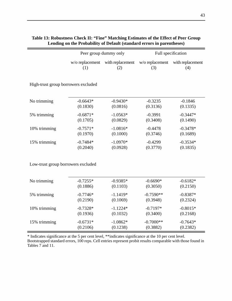
43

ound in
* Indicates significance at the 5 per cent level, **indicates significance at the 10 per cent level.Bootstrapped standard errors, 100 reps. Cell entries represent probit results comparable with those fTables 7 and 11.
Table 13: Robustness Check II: “Fine” Matching Estimates of the Effect of Peer GroupLending on the Probability of Default (standard errors in parentheses)

Peer group dummy only Full specification

w/o replacement(1)

with replacement(2)

w/o replacement(3)

with replacement(4)

High-trust group borrowers excluded

No trimming -0.6643*(0.1830)

-0.9430*(0.0816)

-0.3235(0.3136)

-0.1846(0.1335)

5% trimming -0.6871*(0.1705)

-1.0563*(0.0829)

-0.3991(0.3408)

-0.3447*(0.1490)

10% trimming -0.7571*(0.1970)

-1.0816*(0.1000)

-0.4478(0.3746)

-0.3478*(0.1689)

15% trimming -0.7484*(0.2040)

-1.0970*(0.0928)

-0.4299(0.3770)

-0.3534*(0.1835)

Low-trust group borrowers excluded

No trimming -0.7255*(0.1886)

-0.9385*(0.1103)

-0.6690*(0.3050)

-0.6182*(0.2150)

5% trimming -0.7746*(0.2190)

-1.1419*(0.1069)

-0.7590**(0.3948)

-0.8387*(0.2324)

10% trimming -0.7328*(0.1936)

-1.1224*(0.1032)

-0.7197*(0.3400)

-0.8015*(0.2168)

15% trimming -0.6731*(0.2106)

-1.0862*(0.1238)

-0.7000**(0.3882)

-0.7643*(0.2382)

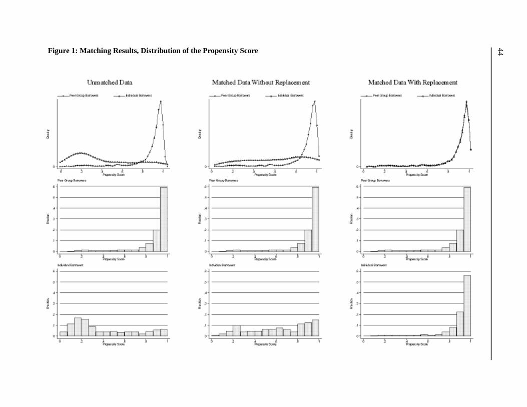
44Figure 1: Matching Results, Distribution of the Propensity Score

45

Figure 2: Trimmed Matching Results, Distribution of the Propensity Score

46Figure 3: Trimmed Matching Results Without Replacement (High-Trust Groups Excluded), Distribution of the Propensity Score

47

Figure 4: Trimmed Matching Results Without Replacement (Low-Trust Groups Excluded), Distribution of the Propensity Score

48

$500

rmat

and

nd

ss the

ach

eral is

rs

ther’s

is not

er

:

re

hased

nts

ated

idual

es.

are

ir

Appendix A: A Note on Calmeadow’s Lending Mechanism

Calmeadow offers two types of loans: group and individual. Group loans range in size from

to $5,000, with $1,000 being the typical loan size for first-time borrowers. The loan term is

typically 12 months and early repayment is an option, with no penalty. The group lending fo

has the following features. Any group of four to seven borrowers can apply for a loan from

Calmeadow, and borrowers must form their group before applying for a loan.1 For the loan

application, group borrowers must provide personal information, references, and business

demographic information on the loan application form. This information must be checked a

approved by all other group members. Group members are encouraged to rigorously asse

credit-worthiness and entrepreneurial competence of their potential peer-group members.

Submission of the group’s loan applications occurs once group members have approved e

other’s applications. Calmeadow loan managers then assess the group’s application; collat

not required, but credit checks are performed. Upon Calmeadow’s approval, group membe

receive their loans all at the same time. Group members, though not strictly liable for each o

loans, are ineligible to access subsequent loans if one group member falls into arrears and

currently “paid up.” In this way, joint liability is implemented.2

Calmeadow also offers individual loans that range in size from $1,000 to $15,000 over long

terms (up to 60 months), and to which anyone can apply.3 The screening process is more rigorous

borrowers must have an existing business over 12 months old, be registered, provide a mo

sophisticated business plan, and occasionally provide collateral (usually, the fixed asset purc

with loan funds).4 Consequently, Calmeadow views individual borrowers as being “better” clie

in terms of loan application requirements. The criteria by which borrowers are sorted into

individual and group loans is explicitly stated in Calmeadow’s promotional literature and repe

during information sessions, before potential borrowers decide whether to apply for an indiv

or group loan.

1. Despite being in a peer-group loan program, all borrowers operate their own individual business2. This requirement is explicitly stated in the “Borrower’s Warrant” and is repeatedly emphasized in

Calmeadow’s promotional literature. Furthermore, when peer group clients fall into arrears, theyreminded that their behaviour will result in their fellow group members’ inability to access futureloans.

3. Unlike many MFIs, Calmeadow does not means test its clients; any individual, regardless of thesocio-economic well-being (unlike the Grameen Bank, for instance, which prevents wealthierindividuals from applying), can apply for a loan.

4. The criterion regarding the age of a business is occasionally relaxed if the individual has self-employment training.

49

s. For

ial

ers,

int

t

re.

The consequences of non-repayment are substantial for both group and individual borrower

group borrowers, failure to repay means that their fellow group members will not be able to

access future loans from Calmeadow and consequently can expect to incur the cost of soc

sanctions imposed by their fellow peer group members. For both group and individual borrow

there are also substantial individual costs to non-repayment (that are independent of the jo

liability costs), because defaulting results in a serious deterioration of that individual’s credi

history and in the submission of the loan claim to a collection agency. This “R9” on the

borrower’s credit history will make them unable to access any formal credit far into the futu

Bank of Canada Working PapersDocuments de travail de la Banque du Canada

Working papers are generally published in the language of the author, with an abstract in both officiallanguages.Les documents de travail sont publiés généralement dans la langue utilisée par les auteurs; ils sontcependant précédés d’un résumé bilingue.

Copies and a complete list of working papers are available from:Pour obtenir des exemplaires et une liste complète des documents de travail, prière de s’adresser à:

Publications Distribution, Bank of Canada Diffusion des publications, Banque du Canada234 Wellington Street, Ottawa, Ontario K1A 0G9 234, rue Wellington, Ottawa (Ontario) K1A 0G9E-mail: [email protected] Adresse électronique : [email protected] site: http://www.bankofcanada.ca Site Web : http://www.banqueducanada.ca

20032003-32 The Canadian Phillips Curve and Regime Shifting F. Demers

2003-31 A Simple Test of Simple Rules: Can They Improve HowMonetary Policy is Implemented with Inflation Targets? N. Rowe and D. Tulk

2003-30 Are Wealth Effects Important for Canada? L. Pichette and D. Tremblay

2003-29 Nominal Rigidities and Exchange Rate Pass-Throughin a Structural Model of a Small Open Economy S. Ambler, A. Dib, and N. Rebei

2003-28 An Empirical Analysis of Liquidity and OrderFlow in the Brokered Interdealer Market forGovernment of Canada Bonds C. D’Souza, C. Gaa, and J. Yang

2003-27 Monetary Policy in Estimated Models of SmallOpen and Closed Economies A. Dib

2003-26 Measuring Interest Rate Expectations in Canada G. Johnson

2003-25 Income Trusts—Understanding the Issues M.R. King

2003-24 Forecasting and Analyzing World Commodity Prices R. Lalonde, Z. Zhu, and F. Demers

2003-23 What Does the Risk-Appetite Index Measure? M. Misina

2003-22 The Construction of Continuity-AdjustedMonetary Aggregate Components J. Kottaras

2003-21 Dynamic Factor Analysis for Measuring Money P.D. Gilbert and L. Pichette

2003-20 The U.S. Stock Market and Fundamentals: AHistorical Decomposition D. Dupuis and D. Tessier

2003-19 A Small Dynamic Hybrid Model for the Euro Area R. Djoudad and C. Gauthier

2003-18 Technological Change and the Education Premiumin Canada: Sectoral Evidence J. Farès and T. Yuen

2003-17 Explaining and Forecasting Inflation in Emerging J. Bailliu, D. Garcés, M. Kruger,Markets: The Case of Mexico and M. Messmacher

2003-16 Some Notes on Monetary Policy Rules with Uncertainty G. Srour