ssr 203 part 2: ranger - rehabilitation - home - · web viewthe first two plots contain waste...

Part 2: Ranger – rehabilitation

107

KKN 2.2.1 Landform design

Revegetation trial demonstration landform – erosion and chemistry studies

MJ Saynor, J Taylor, R Houghton, WD Erskine & D Jones

IntroductionA long-term SSD program of research to assess rainfall, runoff, and sediment and solute losses from a trial rehabilitation landform constructed at the end of 2008 by ERA is expected to proceed for five to ten years. The purpose of the trial landform is to test, over the long term, proposed landform design and revegetation strategies for the site, such that the most appropriate one can be implemented at the completion of mineral processing. While SSD is leading the erosion assessment project, and providing most of the staff resources, there is also a substantial level of assistance and collaboration being provided by technical staff from ERA. SSD is also contributing to the revegetation component of the trial landform by work on vegetation analogue communities.

The trial landform was designed to test two types of potential final cover materials for the rehabilitated mine landform: waste rock and waste rock blended with approximately 30% v/v of fine-grained weathered material (lateritic material). In addition to two different types of cover materials, two different planting methods were implemented: direct seeding and tube stock.

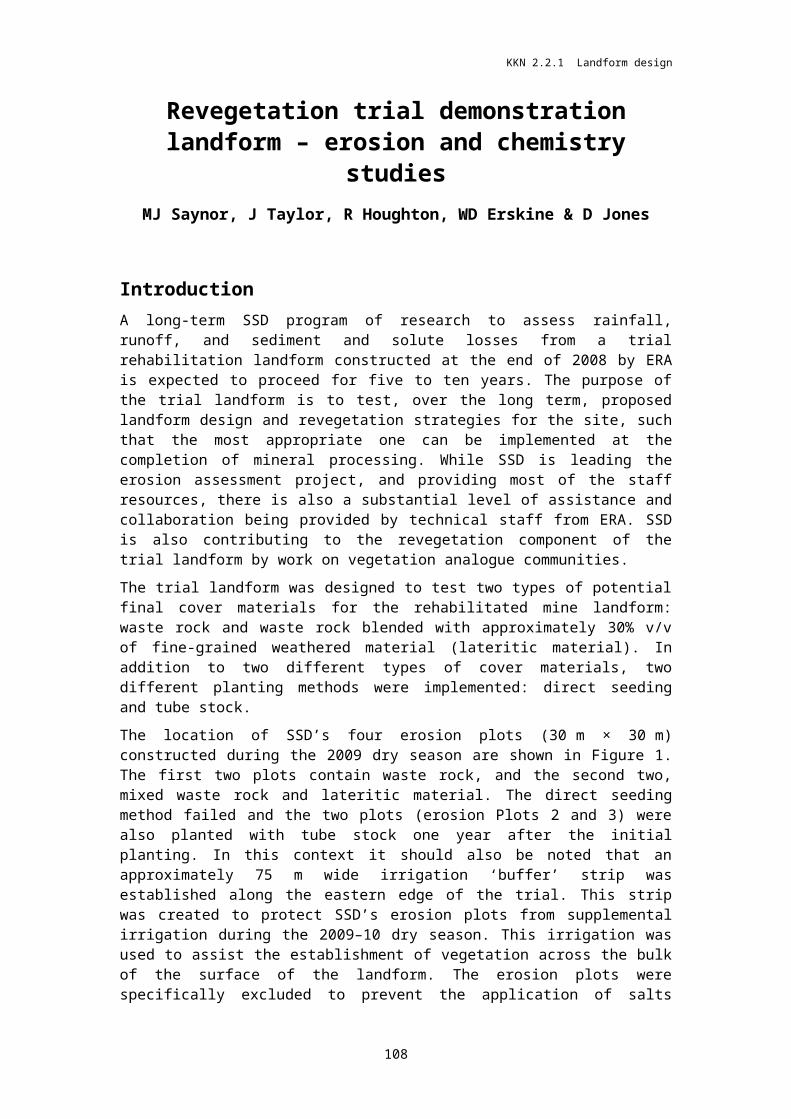
The location of SSD’s four erosion plots (30 m × 30 m) constructed during the 2009 dry season are shown in Figure 1. The first two plots contain waste rock, and the second two, mixed waste rock and lateritic material. The direct seeding method failed and the two plots (erosion Plots 2 and 3) were also planted with tube stock one year after the initial planting. In this context it should also be noted that an approximately 75 m wide irrigation ‘buffer’ strip was established along the eastern edge of the trial. This strip was created to protect SSD’s erosion plots from supplemental irrigation during the 2009–10 dry season. This irrigation was used to assist the establishment of vegetation across the bulk of the surface of the landform. The erosion plots were specifically excluded to prevent the application of salts contained in irrigation water and the complications this would have caused with trying to measure the intrinsic solute loads produced from the cover materials during the subsequent wet season.

Due to the failure of the direct seeding treatment in the first year, and the less than optimal survival of tubestock, all areas on the landform, including all four of the erosion plots, have now been in-fill planted with tube stock. In practice this has meant that the effect of vegetation coverage on erosion rates would likely have been minimal for all four plots over the first two wet seasons.

In this paper the results of rainfall, bedload yields and surface material grain size characteristics for the four erosion plots are reported. Historical staff resourcing issues (as discussed in progress to date below) has meant that the processing of the continuous data for the four erosion plots is not yet complete. Thus water yields, loads of fine suspended sediment and solute loads remain to be derived. These will be derived and reported during the 11/12 work year.

108

Revegetation trial demonstration landform – erosion and chemistry studies (MJ Saynor, J Taylor, R Houghton, WD Erskine & D Jones)

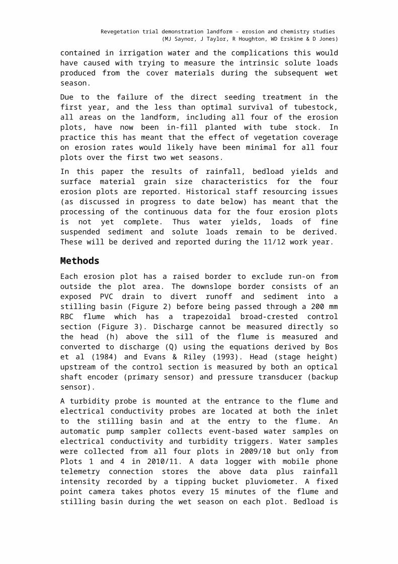
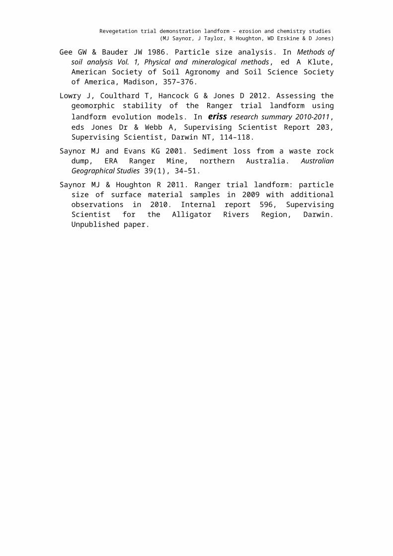
MethodsEach erosion plot has a raised border to exclude run-on from outside the plot area. The downslope border consists of an exposed PVC drain to divert runoff and sediment into a stilling basin (Figure 2) before being passed through a 200 mm RBC flume which has a trapezoidal broad-crested control section (Figure 3). Discharge cannot be measured directly so the head (h) above the sill of the flume is measured and converted to discharge (Q) using the equations derived by Bos et al (1984) and Evans & Riley (1993). Head (stage height) upstream of the control section is measured by both an optical shaft encoder (primary sensor) and pressure transducer (backup sensor).

A turbidity probe is mounted at the entrance to the flume and electrical conductivity probes are located at both the inlet to the stilling basin and at the entry to the flume. An automatic pump sampler collects event-based water samples on electrical conductivity and turbidity triggers. Water samples were collected from all four plots in 2009/10 but only from Plots 1 and 4 in 2010/11. A data logger with mobile phone telemetry connection stores the above data plus rainfall intensity recorded by a tipping bucket pluviometer. A fixed point camera takes photos every 15 minutes of the flume and stilling basin during the wet season on each plot. Bedload is collected manually at least monthly from the PVC drain and from the stilling basin upslope of the flume.

When the discrete water samples collected by the pump samplers are retrieved, predetermined samples (based on measured EC trace) are subsampled for chemical analyses. Electrical conductivity and pH are measured on site for each sample. The aliquots for chemical analysis are stored on ice and transported to the Northern Territory Environmental Laboratories (NTEL) where the following are determined: total nitrogen, total phosphorus, orthophosphate, chloride, aluminium, barium, calcium, copper, iron, potassium, magnesium, manganese, sodium, nickel, lead, sulfate, silica, uranium and zinc. The remainder of the water samples are returned to the eriss laboratory in Darwin where turbidity is measured before the samples are filtered through a 0.45 µm cellulose nitrate filter paper to determine total suspended solids.

Figure 1 Layout of the erosion plots on the trial landform


Figure 2 PVC pipe along lower boundary of Plot 2 leading into the stilling basin immediately upslope of the RBC flume (8 August 2011)

Figure 3 Upstream view of a 200 mm RBC Flume on Plot 2 (2 February 2010) showing float well on right hand side, and Analite NEP395GSV3 turbidity probe and inlet to the Gamet pump sampler at the

entrance to the flume (WD Erskine Photo)

PVC pipe

Tipping Bucket HS TB3 rain gauge

Float well with optical shaft encoder

RBC Flume

Stilling Basin

RBC Flume

Analite turbidity probe and inlet to pump sampler Float well

Exit


A water year that extends from the driest month for 12 consecutive months, instead of being represented by a calendar year, is used to report the results since the use of a calendar year would inappropriately combine data from two different wet seasons. This is because the wet season in the ARR typically extends over a six to seven month period from late October in one year to the end of April in the next (for example, October 2010 to April 2011). To include, within the correct water year, significant rainfall events that can also occur over several weeks at either end of the wet season, a ‘water year’ has been defined as the period from 1 September in the first year to 31 August in the next.

Sediment is transported by flowing water as either suspended load or bedload. Suspended load refers to relatively fine-grained sediment transported in continuous or intermittent suspension, depending on grain size, flow velocity and fluid turbulence. Given that it can be transported in suspension over long distances it is most likely to have a downstream impact on water quality. Bedload is coarse sediment that is best defined as that part of the sediment load that moves on or near the ground surface rather than in the main bulk of overland flow. It stops moving once flow velocity reduces below a critical value. Both suspended and bedload sediment components are being measured as part of this project. The results of the bedload measurements are reported this year, with the suspended sediment data to be reported next year.

Bedload is trapped in either a drain at the down slope end of the plot, or in a deep collection basin (located upstream of the flow measurement flume) at the discharge end of the drain . The sediment from both the drain and basin is combined to form the bedload sample. Bedload samples were collected usually at weekly to monthly intervals during the wet season, or on an as needs basis in response to isolated large rainfall events. The collected samples were transported to the eriss laboratory in Darwin, oven dried and weighed. The grain size distribution for each bedload sample from each plot was determined using a combination of sieve and hydrometer (gravity settling) methods to determine the percentage of gravel (> 2 mm), sand (< 2 mm and > 63 µm), and silt and clay (< 63 µm).

Bulk samples of surface material were collected at 12 sites across the trial landform with two samples collected at each site. One sample was generally collected from between rip lines and the other sample was collected from the top of the mound formed by the rip line. Particle size analysis by the combined hydrometer and sieve method (Gee & Bauder 1986) was undertaken on the 24 samples and graphic grain size statistics calculated from the cumulative frequency distribution (Saynor & Houghton 2011). A software package called ‘Digital Gravelometer’TM was also used to derive particle size distributions from vertical photographs of the surface material at the same sites and the graphic grain size statistics were calculated from the cumulative frequency distribution (Saynor & Houghton 2011). This information is required to run the CAESAR landform evolution model (Lowry et al 2012).

Progress to dateDue to loss of staff, processing of most of the collected data was not possible during the first water year (2009/10). This situation was rectified in 2011 and data processing is now well advanced. All rainfall data for 2009/10 and 2010/11 have been checked and any gaps infilled. Water heights, turbidities and electrical condictivities for Plot 1 have been checked and any gaps infilled for the water years 2009/10 and 2010/11. Work is still in progress for the retrospective cleaning and analysis of the previous two wet season’s data for Plots 2, 3 and 4. All continuously recorded data for the 2011/12 water year are being checked and stored on a weekly basis.


ResultsMeasurements of bedload yields from each plot over the past two water years are presented first followed by information on the particle size characteristics of the surficial material.

Annual bedload yieldsThe bedload yields for each plot for each water year are contained in Table 1. The annual rainfall recorded for each plot for each water year is also shown in Table 1.

Table 1 Yields and particle size distribution of bedload from the four erosion plots for 2009-10 and 2010-2011 water yeras ( September to August inclusive)

Water year Erosion plot Annual rainfall (mm)

Annual bedload yield (t/km2.yr)

% Gravel (> 2 mm)

% Sand (< 2 mm & > 63 µm)

% Silt and clay (< 63 µm)

2009–10 Plot 1 1507 108 34 60 6

2010–11 Plot 1 2246 62 34 63 3

2009–10 Plot 2 1516 143 34 55 11

2010–11 Plot 2 2313 112 41 55 4

2009–10 Plot 3 1480 115 37 59 4

2010–11 Plot 3 2208 57 46 53 1

2009–10 Plot 4 1518 137 35 61 4

2010–11 Plot 4 2319 55 50 49 1

The 2010–11 water year was much wetter than 2009–10, with annual rainfall being between 727 and 801 mm higher on each plot (Table 1). For a given year, bedload yields are similar between both surface cover types and both vegetation planting treatments (Table 1). However, the highest bedload yields were always generated from Plot 2 (Table 1). While it is still not clear why Plot 2 generates the highest yields, shallow rip lines dominate the lower section of the plot resulting in diffuse overland flow connecting with the down slope plot border. Unusually, bedload yields were higher in 2009–10 than in 2010–11 (Table 1). This is consistent with previous research in the Alligator Rivers Region that has shown that sediment yields decline progressively over at least the first three years following a major surface disturbance (Duggan 1988; 1994), such as the construction of an artificial landform. This decrease occurs as a result of initial flushing of fine particles and the formation of an armoured surface. However, it differs from natural land surface environments where sediment yields are usually linearly related to annual runoff or rainfall.

There was a substantial flush of fine sediment (silt and clay) in the 2009–10 water year which had the effect of reducing the supply of this size fraction for the second year (Table 1). Such early preferential removal of fine sediment usually results in an increase in the surface cover of residual gravel via a process called armouring. Concurrently with the development of armouring there is an increase in the percentage gravel in the bedload (Table 1). The data indicate the high rainfall of the 2010–11 water year transported a greater percentage of gravel in comparison to the sand, and silt and clay fractions. Sand was the dominant sediment fraction transported off the erosion plots, consistent with results for other plots on waste rock at the Ranger mine (Table 1)(Saynor & Evans 2001).

The bedload yields for both the first and second year after construction of the trial landform exceeded 55 t.km-2.yr-1 (Table 1). They were high by Australian standards for natural land surfaces, where sediment yields usually range from 4–46 t.km-2.yr-1, but were much less than


the 188–5100 t.km-2.yr-1 recorded for unrehabilitated waste rock stockpiles in the ARR (Erskine & Saynor 2000). This finding highlights the high erodibility of freshly placed waste rock and laterite, and indicates the need for appropriate engineering design of drainage structures and sedimentation basins.

Particle size of surface materialThe results from the sieve and hydrometer method were used for comparisons of graphic grain size statistics between the samples collected between the rip lines and those samples collected at the top of the mound created by the rip line. The results show that for three of the five graphic grain size statistics there was no significant difference between the waste rock and the waste rock mixed with lateritic material. However for graphic mean size and inclusive graphic standard deviation there were significant differences (Saynor & Houghton 2011).

The graphic grain size statistics for the combined hydrometer and sieve method were significantly different to those derived from the ‘Digital Gravelometer’TM. The reasons for the poor correspondence in graphic grain size statistics between the two methods are that the ‘Digital Gravelometer’TM:

is unable to determine the full range of particle sizes as provided by the sieve and hydrometer method;

is unduly influenced by the unevenness of the ground which creates shadows which are wrongly measured as individual clasts;

has problems distinguishing the smaller particles and often aggregated the smaller particles into one large particle; and

had problems recognising individual angular clasts of waste rock (Saynor & Houghton 2011).

Particle size analysis by the combined hydrometer and sieve method provides a better estimation of the size distribution of the particles present on the trial landform surface. It does, however, underestimate the amount of very large particle sizes (>0.5 m in diameter) because it was not physically possible to collect a large enough sample to inclusively contain a sufficiently representative sample of these very large components. To do so would have entailed collecting samples of over 1 t (Gale & Hoare 1992), which would not have been physically practicable given the available sample collection and processing resources.

Future workThe discharge, turbidity, suspended sediment and solute data for the four plots for the first three water years will be progressively collated and analysed over the next wet season. The detailed results will be reported to ARRTC 29 in November 2012. A Supervising Scientist report (SSR) containing the experimental design, plot layout, rainfall, runoff, suspended sediment loads and solute loads for each water year and annual bedload yields will be produced. It is intended to subsequently publish this material in a number of journal papers. The outputs from this project will also provide the means for verifiying the erosion rate time series predictions produced by the CAESAR erosion model (KKN 2.2.1 Landform design- Assessing the geomorphic stability of the Ranger trial landform using landform evolution models).


ReferencesBos MG, Replogle JA & Clemmens AJ 1984. Flow measuring flumes for open channel

systems. John Wiley & Sons, New York.

Duggan K 1988. Mining and erosion in the Alligator Rivers Region of Northern Australia. Unpublished PhD thesis, School of Earth Sciences, Macquarie University.

Duggan K 1994. Erosion and sediment yields in the Kakadu Region of northern Australia. In: Variability in stream erosion and sediment transport. Eds LJ Olive, Loughran RJ, Kesby JA, International Association of Hydrological Sciences, Wallingford, 373–383.

Erskine WD & Saynor MJ 2000. Assessment of the off-site geomorphic impacts of uranium mining on Magela Creek, Northern Territory, Australia. Supervising Scientist Report 156, Supervising Scientist, Darwin NT.

Evans KG & Riley SJ 1993. Regression equations for the determination of discharge through RBC flumes. Internal report 104, Supervising Scientist for the Alligator Rivers Region, Canberra. Unpublished paper.

Gale SJ & Hoare PG 1992. Bulk sampling of coarse clastic sediments for particle size analysis. Earth Surface Processes and Landforms 17, 729–733.

Gee GW & Bauder JW 1986. Particle size analysis. In Methods of soil analysis Vol. 1, Physical and mineralogical methods, ed A Klute, American Society of Soil Agronomy and Soil Science Society of America, Madison, 357–376.

Lowry J, Coulthard T, Hancock G & Jones D 2012. Assessing the geomorphic stability of the Ranger trial landform using landform evolution models. In eriss research summary 2010-2011, eds Jones Dr & Webb A, Supervising Scientist Report 203, Supervising Scientist, Darwin NT, 114–118.

Saynor MJ and Evans KG 2001. Sediment loss from a waste rock dump, ERA Ranger Mine, northern Australia. Australian Geographical Studies 39(1), 34–51.

Saynor MJ & Houghton R 2011. Ranger trial landform: particle size of surface material samples in 2009 with additional observations in 2010. Internal report 596, Supervising Scientist for the Alligator Rivers Region, Darwin. Unpublished paper.

KKN 2.2.1 Landform design

Assessing the geomorphic stability of the Ranger trial landform using landform

evolution modelsJ Lowry, T Coulthard1 & G Hancock0 & D Jones

IntroductionThe Ranger trial landform, located to the northwest of the tailings storage facility (TSF) at Ranger mine, was constructed by Energy Resources of Australia (ERA) during late 2008 and early 2009. The trial landform covers an area of 8 hectares and was built by ERA to test landform design and revegetation strategies to assist in the development of a robust rehabilitation strategy once mining and milling have finished. Specifically, the landform was designed to test two types of potential final cover layers: waste rock alone; and waste rock blended with approximately 30% v/v of fine-grained weathered horizon material (laterite).

During 2009 the Supervising Scientist Division (SSD) constructed four erosion plots (30 m x 30 m) on the trial landform surface, with two plots in the area of waste rock and two in the area of mixed waste rock and laterite (see Figure 1 in previous paper). The plots were physically isolated from runoff from the rest of the landform area by constructed borders.

Field measurements from the erosion plots on the trial landform are being collected over a multi-year period (2009–2014) to support long-term (multi-decadal) assessments of the geomorphic stability of the landform using the CAESAR (Cellular Automaton Evolutionary Slope and River) landform evolution model (LEM). CAESAR (Coulthard 2000, 2002) was originally developed to examine the effects of environmental change on river evolution and to study the movement of contaminated river sediments. Recently, it has been modified to study the evolution of proposed rehabilitated mine landforms in northern Australia (Hancock et al 2010; Lowry et al 2009). The CAESAR model is currently being used to model the erosion from SSDs purpose-built erosion plots located on the trial landform. The predictions of the model are being compared with what is actually being measured through successive wet seasons to provide a validation check on the ability of this model to predict changes in erosion rates through time. The results of modelling performed using field observations collected over 2009–10 are reported here.

MethodsThe model utilises three key data inputs: (1) a digital elevation model (DEM); (2) rainfall data; and (3) surface particle size data.

A DEM of the trial landform was produced from data collected by a Terrestrial Laser Scanner in June 2010. Each of the four erosion plots were scanned at a resolution of 2 cm at a distance of 100 metres. For the purposes of this study, the data for the erosion plots were interpolated to produce a surface grid with a horizontal resolution of 20 cm. The DEMs were rotated by 137o to ensure that drainage flowed from west to east (a CAESAR pre-requisite) and then processed using ArcGIS software to ensure that the DEMs were pit-filled and hydrologically

1 Department of Geography, University of Hull, Hull, HU6 7RX, UK0 School of Environmental and Life Sciences, University of Newcastle, Callaghan, NSW 2308, Australia

115

Assessing the geomorphic stability of the Ranger trial landform using landform evolution models (J Lowry, T Coulthard & G Hancock & D Jones)

corrected. This pit filling was important in order to remove data artefacts, which included remnants of vegetation (peaks) as well as artificial depressions or sinks. Only plots 1 and 2, on a waste rock surface were used for this current study, as the hydrological and suspended sediment data for plots 3 and 4 were not yet available.

Rainfall data were collected individually for each erosion plot using a rain gauge installed at the downstream end of each of the plots.

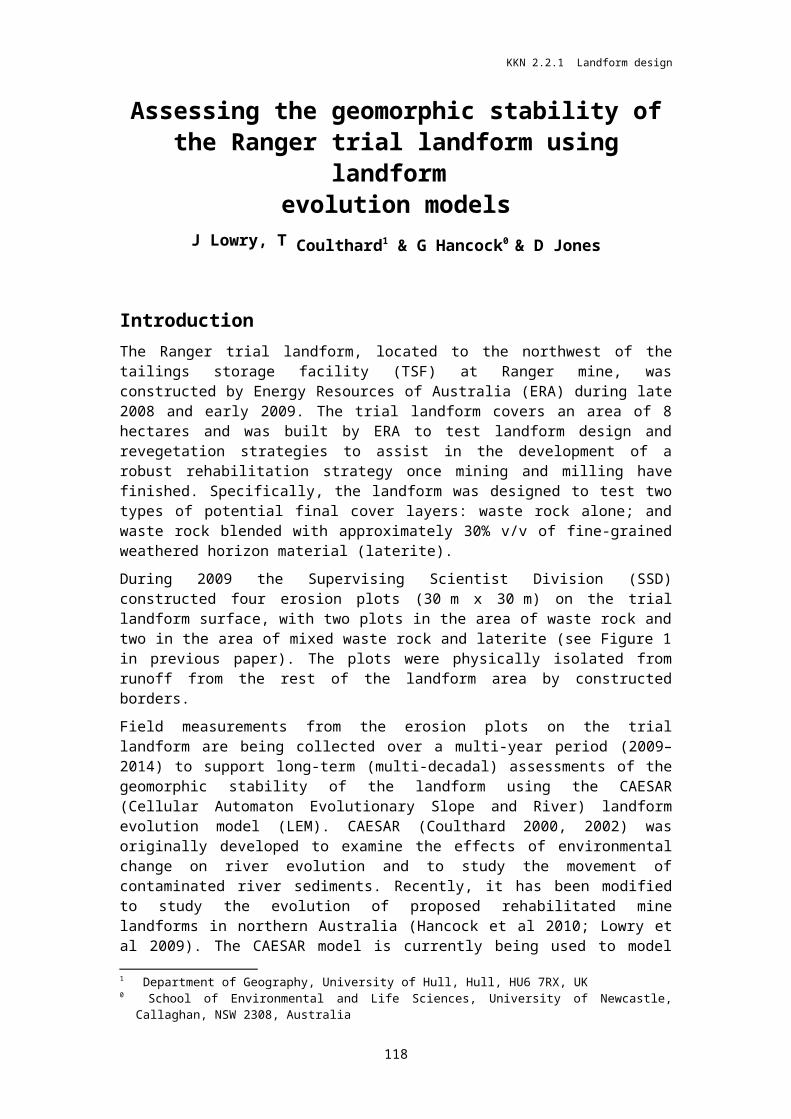
Grain size data for CAESAR were obtained by collecting bulk samples of surface material at eight points within each of the two plots and size fractionating them. Mean values for all eight sites were taken and these means were then re-sampled into nine grain size classes (Figure 1) to be used for input into CAESAR. The sub 0.00063m fraction was treated as suspended sediment within CAESAR.

Figure 1 Grain size distribution for plot 2

The model outputs were compared with field data collected from the outlet of each erosion plot, which was instrumented with a range of sensors. These included a pressure transducer and shaft encoder to measure stage height; a turbidity probe; electrical conductivity probes located at the inlet to the stilling well and in the entry to the flume to provide a measure of the concentrations of dissolved salts in the runoff; an automatic water sampler to collect event based samples; and a data logger with mobile phone telemetry connection.

Three sets of simulations were carried out. The first simulation involved the application of the 2009–2010 wet season data to plot 2, whilst the second simulation involved the application of the 2009–2010 wet season data to plot 1. Finally, the 2009–2010 wet season was repeated 20 times to simulate how the plots would evolve over longer time scales on plot 2. The total volume of sediment for each of the nine grain size classes were recorded from the model every 10 minutes of simulated time along with runoff values. Surface elevations and the distribution of grain sizes for material remaining on the landform surface were recorded every simulated month.

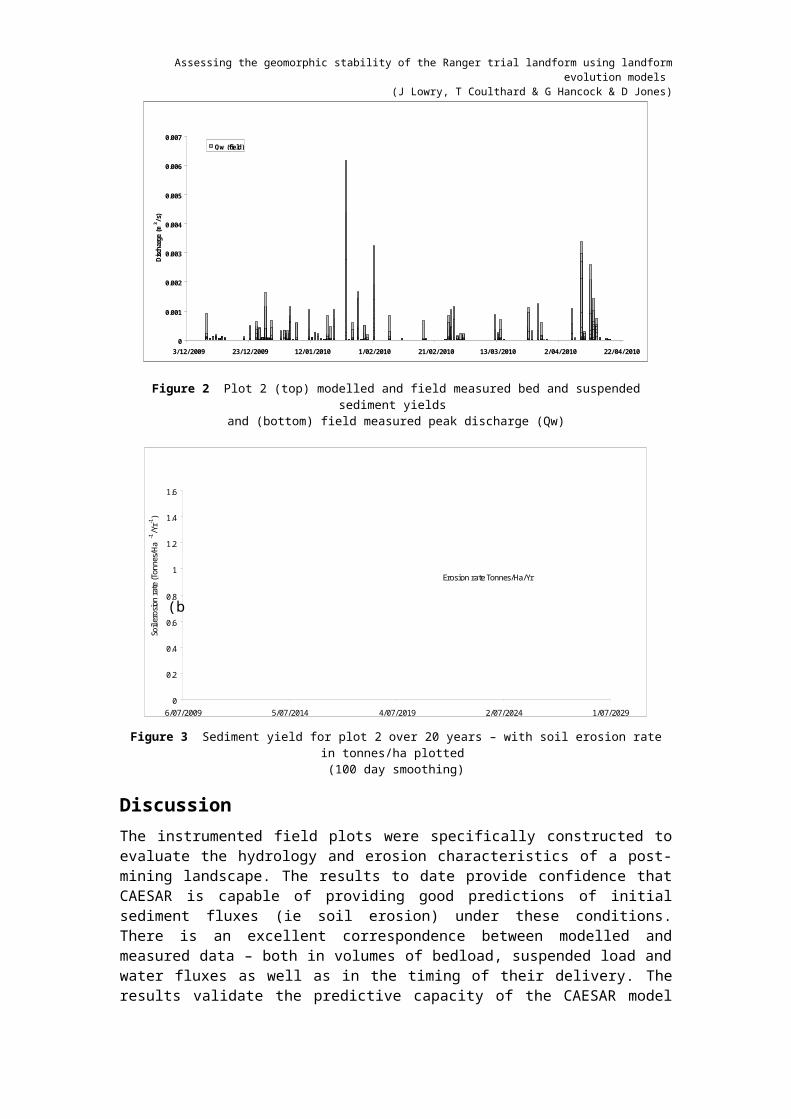
Results/progress to dateFigure 2 shows the results for plot 2 of both modelled and field data for both suspended sediment and bedload results and the measured peak discharge. The modelled and measured bedload and suspended sediment data shows a close correspondence in both volume and timing of increases. The increases in field data are asynchronous with the modelled data as bedload samples were taken sporadically with a typical 2 week frequency compared to the 10 minute output resolution of the model data. Figure 2 also demonstrates a very close similarity between field (solid line) and modelled suspended sediment yields from plot 2. Here, unlike the bedload, the measured suspended sediment data is at the same 10 minute resolution as the


modelled data and an excellent correspondence in terms of timing and magnitude can be seen. Increases in sediment yield correspond to the larger runoff events in the plot.

Due to instrumentation problems there was less processed data available for runoff or suspended sediment from plot 1. As the plots 1 and 2 are 60 metres apart, it was assumed there would be little difference in the rainfall for plot 1. Consequently, the rainfall data for plot 2 was used in the simulations for plot 1. While less processed field data was available, the simulations for plot 1 indicated a very good correspondence between the modelled and observed bedload yields. Also, like plot 2 the field and model data responds mostly to the larger runoff events.

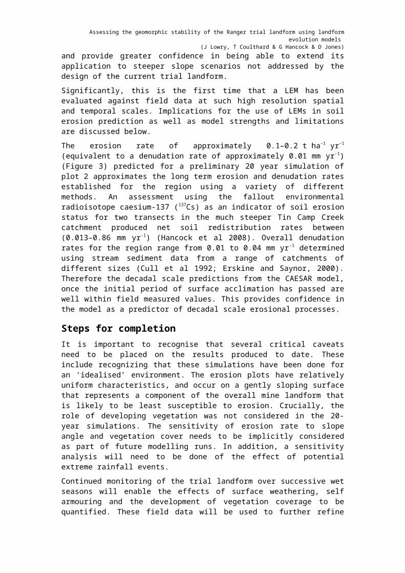
The rainfall sequence from the 2009–2010 wet season was repeated twenty times to produce a hypothetical 20 years simulation of the evolution of plot 2 (Figure 3). This enabled a preliminary assessment to be made of how the rates of sediment loss and the plot morphology may change over this period of time. Figure 3 shows that there is rapid tail off and decrease in sediment yields after the first five years.

0

0.005

0.01

0.015

0.02

0.025

0.03

0.035

0.04

0.045

3/12/2009 23/12/2009 12/01/2010 1/02/2010 21/02/2010 13/03/2010 2/04/2010 22/04/2010

Sedi

men

t Yie

ld (m

3 )

Cumulative Suspended Sediment (field)

Cumulative Suspended Sediment(modelled)Cumulative Bedload (modelled)

Cumulative Bedload (field)

0

0.001

0.002

0.003

0.004

0.005

0.006

0.007

3/12/2009 23/12/2009 12/01/2010 1/02/2010 21/02/2010 13/03/2010 2/04/2010 22/04/2010

Disc

harg

e (m

3 /s)

Qw (field)

Figure 2 Plot 2 (top) modelled and field measured bed and suspended sediment yields and (bottom) field measured peak discharge (Qw)


Soil

eros

ion

rate

(Ton

nes/

Ha-1

/Yr-1

)

0

0.2

0.4

0.6

0.8

1

1.2

1.4

1.6

6/07/2009 5/07/2014 4/07/2019 2/07/2024 1/07/2029

Erosion rate Tonnes/Ha/Yr

Figure 3 Sediment yield for plot 2 over 20 years – with soil erosion rate in tonnes/ha plotted (100 day smoothing)

DiscussionThe instrumented field plots were specifically constructed to evaluate the hydrology and erosion characteristics of a post-mining landscape. The results to date provide confidence that CAESAR is capable of providing good predictions of initial sediment fluxes (ie soil erosion) under these conditions. There is an excellent correspondence between modelled and measured data – both in volumes of bedload, suspended load and water fluxes as well as in the timing of their delivery. The results validate the predictive capacity of the CAESAR model and provide greater confidence in being able to extend its application to steeper slope scenarios not addressed by the design of the current trial landform.

Significantly, this is the first time that a LEM has been evaluated against field data at such high resolution spatial and temporal scales. Implications for the use of LEMs in soil erosion prediction as well as model strengths and limitations are discussed below.

The erosion rate of approximately 0.1–0.2 t ha-1 yr-1 (equivalent to a denudation rate of approximately 0.01 mm yr-1) (Figure 3) predicted for a preliminary 20 year simulation of plot 2 approximates the long term erosion and denudation rates established for the region using a variety of different methods. An assessment using the fallout environmental radioisotope caesium-137 (137Cs) as an indicator of soil erosion status for two transects in the much steeper Tin Camp Creek catchment produced net soil redistribution rates between (0.013–0.86 mm yr-1) (Hancock et al 2008). Overall denudation rates for the region range from 0.01 to 0.04 mm yr-1 determined using stream sediment data from a range of catchments of different sizes (Cull et al 1992; Erskine and Saynor, 2000). Therefore the decadal scale predictions from the CAESAR model, once the initial period of surface acclimation has passed are well within field measured values. This provides confidence in the model as a predictor of decadal scale erosional processes.

Steps for completionIt is important to recognise that several critical caveats need to be placed on the results produced to date. These include recognizing that these simulations have been done for an ‘idealised’ environment. The erosion plots have relatively uniform characteristics, and occur


on a gently sloping surface that represents a component of the overall mine landform that is likely to be least susceptible to erosion. Crucially, the role of developing vegetation was not considered in the 20-year simulations. The sensitivity of erosion rate to slope angle and vegetation cover needs to be implicitly considered as part of future modelling runs. In addition, a sensitivity analysis will need to be done of the effect of potential extreme rainfall events.

Continued monitoring of the trial landform over successive wet seasons will enable the effects of surface weathering, self armouring and the development of vegetation coverage to be quantified. These field data will be used to further refine the relevant algorithms in the CAESAR model and increase confidence in its ability to make more robust longer-term predictions of rates of erosion from rehabilitated mine landforms.

AcknowledgmentsMike Saynor, Annamarie Beraldo, Richard Houghton and Sam Fisher are thanked for their assistance in collecting and processing the data used in this study. Nigel Peters of Sinclair Knight Merz is is thanked for his assistance in generating the DEM of the trial landform.

ReferencesCoulthard TJ, Kirkby MJ & Macklin MG 2000. Modelling geomorphic response to

environmental change in an upland catchment. Hydrological Processes 14, 2031–2045.

Coulthard TJ, Macklin MG & Kirkby MJ 2002. Simulating upland river catchment and alluvial fan evolution, Earth Surface Processes and Landforms. 27, 269–288.

Cull R, Hancock G, Johnston A, Martin P, Marten R, Murray AS, Pfitzner J, Warner RF & Wasson RJ 1992. Past, present and future sedimentation on the Magela plain and its catchment. Modern sedimentation and late Quaternary evolution of the Magela Creek plain. Research report 6, Supervising Scientist for the Alligator Rivers Region, AGPS, Canberra, 226–268.

Erskine WD & Saynor MJ 2000. Assessment of the off-site geomorphic impacts of uranium mining on Magela Creek, Northern Territory, Australia. Supervising Scientist Report 156, Supervising Scientist, Darwin NT.

Hancock GR, Loughran RJ, Evans KG & Balog R 2008. Estimation of soil erosion using field and modelling approaches in an undisturbed Arnhem Land catchment, Northern Territory, Australia. Geographical Research 46(3), 333–349.

Hancock GR, Lowry JBC, Coulthard TJ, Evans KG & Moliere DR 2010. A catchment scale evaluation of the SIBERIA and CAESAR landscape evolution models. Earth Surface Processes and Landforms, 35, 863–875.

Lowry JBC, Evans KG, Coulthard TJ, Hancock GR & Moliere DR 2009. Assessing the impact of extreme rainfall events on the geomorphic stability of a conceptual rehabilitated landform in the Northern Territory of Australia. In Mine Closure 2009. Proceedings of the Fourth International Conference on Mine Closure 9–11 September 2009, eds Fourie A & Tibbett M, Australian Centre for Geomechanics, Perth, 203–212.

KKN 2.2.5 Radiological characteristics of the final landform

Pre-mining radiological conditions at Ranger mine

A Bollhöfer, A Beraldo, K Pfitzner & A Esparon

IntroductionBefore mining started at Ranger in 1981, orebodies 1 and 3 were outcropping in places and several other radiation anomalies were also known to exist in the area. Compared with typical environmental background radiological conditions, these areas exhibited naturally higher soil uranium and radium concentrations and, consequently, elevated gamma ray fields detected by airborne radiometric surveys. From a radiological perspective, assessing the success of mine site remediation at a uranium mine is based upon comparison with the pre-mining radiation levels. It is recommended by the International Commission on Radiation Protection (ICRP 2007) that the annual effective radiation dose above pre-mining levels to a member of the public from practices such as U mining should not exceed 1 milli Sievert. To establish reference radiological conditions for the Ranger mine it is therefore important to have a robust knowledge of the magnitude and spatial extent of the areas that exhibited naturally elevated radiation levels pre-mining.

Airborne gamma surveys (AGS), coupled with groundtruthing measurements, have been used previously for area wide assessments of radiological conditions at remediated and historic mine sites in the ARR (Pfitzner et al 2001a,b, Martin et al 2006, Bollhöfer et al 2008). Using historic AGS data can provide a means to infer pre-mining conditions, if the airborne data can be calibrated using an existing undisturbed/unmined radiological anomaly that was also covered by the original AGS. Whilst a pre-mining AGS was flown over the Alligator Rivers Region, including the Ranger site, in 1976, no ground radiological data of the resolution and spatial coverage needed to calibrate the AGS data are available from that time. In this project data from a high resolution ground survey collected between 2007 and 2009 at an undisturbed radiologically anomalous area have been used to calibrate the AGS data from 1976 for that anomaly. The calibrated AGS data set was then used to infer pre-mining radiological conditions for various altered landform features on site.

MethodsData from the 1976 Alligator Rivers Geophysical Survey, acquired from Rio Tinto by the NT Government, were re-processed in 2000 by the Northern Territory Geological Survey (NTGS) and then re-sampled at a pixel size of 70 × 70 m2 in 2003. This data set is available in the public domain and was used to identify Anomaly 2, about 1 km south of the Ranger lease, as the most suitable undisturbed area to be used for groundtruthing (Esparon et al 2009). It exhibits a strong airborne gamma signal, has not been mined, nor is it influenced by operations associated with the mine. Energy Resources of Australia (ERA) has also provided to SSD higher resolution data from an AGS that was flown in 1997. The Anomaly 2 component of this dataset was used to further refine the extensive groundtruthing fieldwork, conducted in the dry seasons 2007 to 2009, and to establish the exact location and radiological intensity of the Anomaly.

120

Pre-mining radiological conditions at Ranger mine (A Bollhöfer, A Beraldo, K Pfitzner & A Esparon)

More than 1800 external gamma dose rate measurements were made at 1 m height above the ground, to characterise the footprint of Anomaly 2, using conventional GM tubes. These measurements were complemented by the determination of soil uranium, thorium and potassium activity concentrations, via in situ gamma spectrometry, at 150 sites. Dry season radon exhalation rates were measured at 25 sites over a period of three days, and soil scrape samples were taken at these sites for high resolution gamma spectrometry analysis in the eriss radioanalytical laboratory. Track etch detectors were also deployed at these sites for three months to measure dry season airborne radon concentration and to establish whether there is a correlation between airborne radon concentration, radon exhalation flux and soil 226Ra activity concentrations.

Differences in survey parameters of the AGS and on ground datasets, such as field of view of the detectors, detector calibration, spatial referencing and data processing means that the data sets are not directly comparable. In order to be able to compare data collected on ground with the AGS data, upscaling is required of the data measured on ground. Due to the much better resolution and lower flying height of the 1997 AGS the groundtruthed data was firstly upscaled and correlated with the 1997 AGS subset above Anomaly 2. The 1997 and 1976 AGS datasets were then correlated, using the data acquired over the whole extent of the 1997 AGS (which is smaller than the extent of the 1976 Alligator Rivers Geophysical Survey) but excluding the footprint of the mine site. This was done in a GIS environment and results are presented below.

ResultsCorrelating the 1997 AGS and ground dataThe AGS data originally received as projected coordinates of the Australian geodetic datum 1984 were reprojected into the WGS84 map datum, UTM Zone 53S. A shapefile was then created, defined by the boundary of the 2007–09 field data obtained for the Anomaly 2 area (Figure 1). Airborne gamma survey points acquired in 1997 within this boundary were extracted and line segments created between points, representing the plane’s flight path. These line segments were assigned the total counts (TC) and counts in the uranium channel (eU) of the corresponding AGS records.

To upscale the field data, a series of buffers with varying radii were created around the line segments of the 1997 AGS data. The buffer radii were then changed to find the radius that provided the best correlation between the AGS data along that line segment (TC and eU, respectively) and the external gamma dose rates measured in the field (μGy·hr -1) and averaged across the respective buffer. To ensure that results were not affected by variations in field sample spacing, 29 buffers in which ground points were evenly distributed were chosen for further analysis (see Figure 1). It was found that a 90 m buffer radius provided the best correlation (R2=0.76; n = 29; p<0.001; Figure 2) and, thus, represented the optimal field of view for the 1997 dataset.

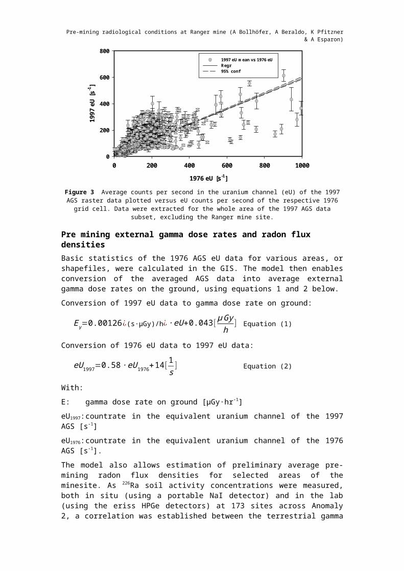
Correlating the 1976 and 1997 AGS dataThe two AGS raster datasets were displayed in projected coordinates of the WGS84 map datum, UTM Zone 53S, and a subset of the raster data was created. This subset incorporated the full extent of the 1997 AGS raster dataset excluding the footprint of the mine site. The 1997 raster data supplied by ERA (25 × 25 m2 resolution) was then correlated with the 1976 raster data (70 × 70 m2 resolution) of this subset, by averaging the 1997 data contained within a 1976 grid cell, and then comparing the average with the eU and TC of the 1976 grid cell (R2=0.65; n=6916; p<0.001; Figure 3).


Figure 1 Shapefile created in ArcGIS for the 2007-2009 ground survey (grey) and buffers chosen to establish the correlation between the ground survey and the 1997 AGS data

eU [s-1] 1997

0 200 400 600 800 1000

Gy/

hr

0.0

0.2

0.4

0.6

0.8

1.0

1.2

1.4

mean uGy/hr vs U Regr95% conf

Figure 2 Averaged ground gamma dose rates within a 90 m buffer radius along the 1997 AGS line segments plotted versus counts per second in the uranium channel (eU) of the respective AGS record


1976 eU [s-1]

0 200 400 600 800 1000

1997

eU

[s-1

]

0

200

400

600

8001997 eU mean vs 1976 eU Regr95% conf

Figure 3 Average counts per second in the uranium channel (eU) of the 1997 AGS raster data plotted versus eU counts per second of the respective 1976 grid cell. Data were extracted for the whole area of

the 1997 AGS data subset, excluding the Ranger mine site.

Pre mining external gamma dose rates and radon flux densitiesBasic statistics of the 1976 AGS eU data for various areas, or shapefiles, were calculated in the GIS. The model then enables conversion of the averaged AGS data into average external gamma dose rates on the ground, using equations 1 and 2 below.

Conversion of 1997 eU data to gamma dose rate on ground:

E γ=0.00126 ¿(s∙µGy)/h¿ ∙ eU+0.043 [ µGyh

] Equation (1)

Conversion of 1976 eU data to 1997 eU data:

eU 1997=0.58∙ eU 1976+14 [ 1s] Equation (2)

With:

E: gamma dose rate on ground [µGy·hr-1]

eU1997: countrate in the equivalent uranium channel of the 1997 AGS [s-1]

eU1976: countrate in the equivalent uranium channel of the 1976 AGS [s-1].

The model also allows estimation of preliminary average pre-mining radon flux densities for selected areas of the minesite. As 226Ra soil activity concentrations were measured, both in situ (using a portable NaI detector) and in the lab (using the eriss HPGe detectors) at 173 sites across Anomaly 2, a correlation was established between the terrestrial gamma dose rate and the 226Ra soil activity concentration. In addition, a correlation was established between radon flux densities and 226Ra soil activity concentrations, and has been reported previously (Bollhöfer et al 2010). Figure 4 shows the 226Ra soil activity concentration plotted versus the terrestrial gamma dose rate, and the measured radon flux densities plotted versus 226Ra soil activity concentration.

Using these correlations, average gamma dose rates and radon flux densities for various areas on the greater Ranger region can be calculated. The minimum footprint area that can be assessed is set by the optimum buffer radius determined when up-scaling the external gamma


dose rates measured on the ground to the AGS data. For the current case this is approximately 4 ha.

Eterr [microGy/hr]0 1 2 3 4 5

226 R

a [B

q/kg

]

0

2000

4000

6000

8000

10000

12000

226Ra = 2341 * Eterr

R2=0.88p<<0.001 A

226Ra [Bq/kg]

10 100 1000 10000 100000

rado

n [m

Bq/

m2 /s]

1

10

100

1000

10000loamy sand fine gravelAnomaly 14

15

1324

16

Rn = (2.20+-0.96)*Ra

R2 = 0.55p < 0.005

B

Figure 4 Preliminary correlations established between (A) 226Ra soil activity concentration and terrestrial gamma dose rate (Eterr) and (B) radon flux density and 226Ra soil activity concentration. For

more explanation see Bollhöfer et al (2010).

Figure 5 shows a 1964 aerial photo that incorporates the greater Ranger mine area. The footprints of some of the currently existing mine site features have been overlaid for reference. The right hand side of the figure displays the 1976 eU data over the same area, with bright colours indicating areas of elevated radiation levels, and darker colours indicating environmental background values.

TDPit 1

Pit 3

RP1

TDPit 1

Pit 3

RP1

Figure 5 Footprints of major infrastructure features on site (A) overlaid on an aerial photo of the greater Ranger mine area from 1964 and (B) overlaid on the 1976 AGS eU data.

RP1: Retention Pond 1; TD: Tailings Dam.

The average counts for each of the outlined areas, or shapefiles, have been determined using our GIS and converted to average external gamma dose rates and radon flux densities using correlations described above. Table 1 shows the estimated pre-mining external gamma dose rates and radon flux densities for each of these marked areas.

Table 1 Estimated pre-mining external gamma dose rates and radon flux densities for areas marked on Figure 5

Infrastructure Area[ha]

γ-dose rate[μGy·hr-1]

Radon flux density[mBq·m-2·s-1]

Tailings Dam 110 0.11 0.19

RP1 17 0.10 0.16

A B


Pit 1 40 0.87 4.1

Pit 3 77 0.44 1.9

The typical environmental background gamma dose rate determined for the whole extent of the 1976 AGS data set and using the derived correlation is approximately 0.1 μGy·hr-1. This compares well with typical background gamma dose rates published for the ARR, ranging from 0.08 to 0.15 μGy·hr-1. The modelled pre-mining gamma dose rates and radon flux densities for orebodies 1 and 3 are also in very good agreement with published values determined using drill cores from orebody 1 and measured on top of orebody 3, respectively (Kvasnicka & Auty 1994). Gamma dose rates and radon flux densities at Ranger reported by Kvasnicka and Auty (1994) were 0.95 μGy·hr-1 and 4.1 mBq·m- 2·s-1 for orebody 1 (44 ha) and 0.58 μGy·hr-1 and 2.5 mBq·m-2·s-1 for orebody 3 (66 ha). Typical background values reported for the Ranger mine area were 0.13 μGy·hr-1 and 0.13 mBq·m-2·s-1, respectively.

ConclusionsThe correlation models developed by this project allow estimates to be made of the pre-mining baseline gamma dose rates and radon fluxes for any selected area (4 ha minimum) covered by the pre mining 1976 AGS data available over the greater Ranger area. The models, in particular the calculation of the radon flux densities, still require some refinement and incorporation of associated uncertainties, both from fitting the data and GIS model asumptions. Nonetheless it is a useful tool already, and a comparison with published data shows that the model estimates are similar to radiation levels estimated previously via direct measurement on top of orebody 3, and estimates made using uranium activity concentrations in drill cores from orebody 1.

Our model will also allow prediction of pre-mining uptake of uranium series radionuclides into biota over the footprint of the Ranger mine, assuming secular equilibrium of the radionuclides in soils and using uptake factors determined for bushtucker in the region. This will facilitate the calculation of pre mining ingestion doses from bushtucker harvested from the site, in addition to the internal and external radiation doses to the environment. The inhalation pathway needs to be quantified, using existing measurements of airborne radon concentrations on top of Anomaly 2 and dust re-suspension factors, which will then enable derivation of the total pre-mining radiological exposure to humans from all pathways.

AcknowledgmentsJared Selwood, Alan Hughes, Rocky Cahill and Gary Fox are thanked for assistance in the field. The Northern Territory Geological Survey and ERA are thanked for the provision of the 1976 and 1997 AGS data, respectively. Thanks to the Mirrar people for allowing access to the sites.

ReferencesBollhöfer A, Pfitzner K, Ryan B, Martin P, Fawcett M & Jones DR 2008. Airborne gamma

survey of the historic Sleisbeck mine area in the Northern Territory, Australia, and its use for site rehabilitation planning. Journal of Environmental Radioactivity 99, 1770–1774.

Bollhöfer A, Esparon A & Pfitzner K 2011. Pre-mining radiological conditions at Ranger mine. In eriss research summary 2009–2010. eds Jones DR & Webb A, Supervising Scientist Report 202, Supervising Scientist, Darwin NT, 101–106.


Esparon A, Pfitzner K, Bollhöfer A & Ryan B 2009. Pre-mining radiological conditions at Ranger mine. In eriss research summary 2007–2008. eds Jones DR & Webb A, Supervising Scientist Report 200, Supervising Scientist, Darwin NT, 111–115.

ICRP 2007. The 2007 Recommendations of the International Commission on Radiological Protection. International Commission on Radiological Protection Publication 103, Elsevier Ltd.

Martin P, Tims S, McGill A, Ryan B & Pfitzner K 2006. Use of airborne -ray spectrometry for environmental assessment of the rehabilitated Nabarlek uranium mine, northern Australia. Environmental Monitoring and Assessment 115, 531–553.

Pfitzner K, Ryan B, Bollhöfer & Martin P 2001a. Airborne gamma survey of the upper South Alligator River valley: Third Report. Internal Report 383, Supervising Scientist, Darwin.

Pfitzner K, Martin P & Ryan B 2001b. Airborne gamma survey of the upper South Alligator River valley: second report. Internal report 377, Supervising Scientist for the Alligator Rivers Region, Darwin.

KKN 2.2.5 Radiological characteristics of the final landform

Radon exhalation from a rehabilitated landformA Bollhöfer & J Pfitzner

IntroductionClosure criteria for the rehabilitation of the Ranger Uranium Mine need to incorporate radiological aspects to ensure that exposure of the public to radiation after rehabilitation of the mine is as low as reasonably achievable. As the inhalation of radon decay products is likely to be a significant contributor to radiological dose particularly in the vicinity of the rehabilitated landform, radon exhalation from the landform and its temporal variability need to be estimated. The radon exhalation rate may potentially change as the final landform evolves after rehabilitation of the site. At the Nabarlek site for instance, differences in radon flux densities measured immediately (Kvasnicka 1996) and 5 years after rehabilition (Bollhöfer et al 2006) have been reported, although these differences could also be due to differences in experimental design between the two studies, as pointed out in Bollhöfer et al (2006). Consequently, opportunities have been sought to provide long-term data about the variation in radon exhalation flux densities from relevant areas of the Ranger minesite. In particular, ERA’s trial landform (Saynor et al 2009) provides a unique opportunity to track radon exhalation over many years. The project will enable eriss and ERA to more confidently predict a long-term radon exhalation flux from a rehabilitated landform and contribute to the development of closure criteria for the site.

The objective of this project is to determine radon (222Rn) exhalation flux densities for various combinations of cover types (two) and re-vegetation strategies (two) on the trial landform and to investigate seasonal and long-term changes in radon exhalation. Specifically, the 222Rn exhalation from the four erosion plots (30 m 30 m) constructed by SSD (Saynor et al 2010) will be measured over several years to investigate whether there are any temporal changes of radon exhalation, taking into account rainfall, weathering of the rock, erosion and compaction effects, and the effect of developing vegetation on the landform.

MethodsConventional charcoal canisters (or ‘radon cups) are used to measure radon exhalation flux densities. The charcoal canisters used are a standard brass cylindrical design with an internal diameter of 0.070 m, depth 0.058 m and a wall thickness of 0.004 m. Details on the charcoal canister methodology are provided in Bollhöfer et al (2003) and Lawrence (2006).

Construction of the trial landform was completed late in the 2008–09 wet season. Since then, irrigation water has been regularly applied to all areas apart from a 40 m buffer strip that contains the SSD erosion plots. As soil moisture content has a substantial effect on radon exhalation, and because the irrigation water may contain significant concentrations of radium, radon exhalation flux density is measured from the four SSD erosion plots only, which are not irrigated nor affected by spray drift from the irrigation (Saynor, pers comm).

To obtain a true average radon exhalation flux density from the uneven and heterogeneous surface of the four erosion plots, radon cups are placed randomly over the surface. One experimenter throws a bag filled with sand over his shoulder, while the second experimenter notes where the bag first hit the ground, this being the selected location for charcoal cup

127

Radon exhalation from a rehabilitated landform (A Bollhöfer & J Pfitzner)

placement. If placed on rocks, the rim of the charcoal cup is sealed using putty. This is in contrast to many other studies where radon cups are placed at ‘convenient’ locations where they can easily be embedded into the finer grained soil. Fine grained material exhibits higher radon flux densities than solid rock (Lawrence et al 2009). Hence, results of radon exhalation measurements can potentially be skewed if the sampling design is not random (Bollhöfer et al 2006).

The location and a description of the four erosion plots where measurements are being taken are shown on Figure 1 and in Table 1, respectively, and are further described in Saynor et al (2010). Generally, 15–20 radon cups are deployed randomly across each erosion plot and are exposed for 3 to 4 days. The charcoal cups are collected after exposure, sealed and sent to the SSD Darwin laboratories, where they are analysed using a NaI gamma detector.

Figure 1 Locations of the radon exhalation measurements conducted from May 2009 to September 2011 overlaid on an aerial photo of the trial landform from October 2010. Different coloured dots

represent locations for the various years.

Progress to dateRadon cups were deployed before the trial landfrom was contructed to determine the radon exhalation from the substrate underlying the constructed landform. Radon flux densities from the pre-construction substrate follow a log-normal distribution with a range from 24 to 144 mBq∙m-2∙s-1 and geometric mean and median both equal to 73 mBq∙m -2∙s-1. This is similar to the average (±1SD) late dry season radon flux density of 64 ±25 mBq∙m-2∙s-1, which was previously determined for the region (Todd et al 1998).

Radon exhalation flux density measurements on the trial landform now cover two seasonal cycles. A summary of the results is presented in Figure 2 and Table 1.


Oct 11May 11Jan 11Sep 10May 10Feb 10Sep 09May 09

700

600

500

400

300

200

100

0

rado

n flu

x de

nsity

[m

Bq/m

2/s]

Plot 1Plot 2Plot 3Plot 4

Plot

Boxplot of May 09, Sep 09, Feb 10, May 10, Sep 10, Jan 11, May 11, Oct 11

Figure 2 Boxplots of radon flux density measurements conducted on the trial landfrom from May 2009 to October 2011, showing median (middle line), 1st (bottom line) and 3rd (top line) quartiles. The upper

(lower) whiskers extend to the maximum (minimum) data point within 1.5 box heights from the top (bottom) of the box. The data points indicate outliers that fall beyond the whiskers.

Table 1 Description of the four erosion plots and average (arithmetic and geometric) radon flux densities measured on the surface in 2009–11

Treatment 222Rn flux density [mBq∙m-2∙s-1]Arithmetic (geometric) average ± error (95% confidence)

May 2009

Sep 2009

Feb 2010

May 2010

Sep 2010

Jan 2011

May 2011

Sep 2011

RUM_EP1 Waste rock material planted with tube stock

22(14) ± 11

14(7) ± 8

7(4) ± 3

43(21) ± 25

60(26) ± 47

100(27) ± 76

60(18) ± 63

68(24) ± 47

RUM_EP2 Waste rock planted by direct seeding

42(27) ± 15

15(7) ± 9

8(5) ± 4

45(28) ± 20

69(36) ± 35

126 (44) ± 86

67(38) ± 37

82(43) ± 43

RUM_EP3 30% laterite/ waste rock mix, direct seeding

18(13) ± 7

14(9) ± 8

5(NA) ± 2

51(21) ± 35

102(78) ± 36

49(NA) ± 48

65(37) ± 33

63(49) ± 19

RUM_EP4 30% laterite/ waste rock mix, tube stock

18(14) ± 7

40(19) ± 32

6(3) ± 4

83(42) ± 51

111(68) ± 60

70(NA) ± 47

71(55) ± 22

112(79) ± 41

Radon flux density measurements show a tendency for some higher values and greater variability over time, in particular in September 2010 and January 2011, and were lowest in the first 12 months of the study. Although the radon exhalation showed a seasonal variation typical of the region (Lawrence et al 2009) in the first year of our measurements, with radon exhalation flux densities lower during the wet season compared to the dry season, radon flux density measurements conducted in January 2011 were higher than in the previous wet season, and highest overall on the waste rock treatment (erosion plots 1 and 2).

Figure 3 shows the median of the radon flux density measurements conducted on the four erosion plots plotted versus the date. The daily rainfall measured on the trial landform is shown for reference.


0

20

40

60

80

100

120

140

15/4/2009 15/8/2009 15/12/2009 15/4/2010 15/8/2010 15/12/2010 15/4/2011 15/8/2011

[mB

q/m

2 /s]

date

rainfallPlot 1Plot 2Plot 3Plot 4

120

80

100

60

40

20

rainfall [mm

]

Figure 3 Median radon flux density measured on the four erosion plots and average daily rainfall measured at the trial landform, plotted versus the date

After two years of radon exhalation measurements, it appears that radon exhalation during the dry season is slightly higher from the laterite/waste rock mix landform as compared to waste rock only. This may simply be a result of higher 226Ra activity concentrations in the material used for construction of plots 3 and 4. However, recent 226Ra soil activity concentration measurements conducted on surface material and erosion products collected from the troughs and basins around the erosion plots discount this hypothesis (Bollhöfer & Pfitzner 2011). A detailed gamma survey of the Trial Landform will help to determine the magnitude of the differences in soil radioactivity between the individual plots, and also show within plot variability of soil radioactivity.

Another reason for the higher dry season radon exhalation may be the smaller average particle size in the laterite/waste rock mix erosion plots. The average percentage of silts and clays (< 63 µm) in surface soils from the laterite/waste rock mix on the Trial Landform is slightly higher at 11% compared to the average percentage in waste rock material only used for the construction of plots 1 and 2 (7%) (Saynor & Houghton, 2011). In contrast, the average percentage gravel (> 2mm) is higher for waste rock only at 67% as compared to 61% for the waste rock-laterite mix. Radon exhalation from smaller sized particles is generally higher for equivalent mass 226Ra activity concentrations (Lawrence et al 2009) and this may explain the higher dry season radon flux densities.

On the other hand, the larger amount of clays in plots 3 and 4 will decrease porosity and lead to waterlogging after rainfall, accompanied by lower radon flux densities during the wet season. Waterlogged areas on plots 3 and 4 were observed when radon cups were deployed between 7-10 January 2011. During this period an average of 20 mm of rain fell each day, with the 4 days prior to radon cup deployment being relatively dry (< 1.5 mm of rain). This water did not drain in some areas of plots 3 and 4, whereas the higher porosity of waste rock material only allowed the rain to infiltrate and no waterlogging was observed at erosion plots 1 and 2.

It has previously been reported that short duration but intense tropical rain events can lead to an increase in radon exhalation, as more radon is then effectively trapped in the soil porewater and released upon evaporation of the water (Lawrence et al 2009). This process may partly explain the high radon flux densities observed for waste rock only plots 1 and 2 on 7–10 January 2011.


Radon exhalation from Plot 2 is generally higher than radon exhalation from Plot 1, which can be explained by the higher 226Ra activity concentration of surface material between the two plots (Bollhöfer & Pfitzner 2011).

Future workRadon exhalation surveys across the four erosion plots will continue to be conducted every 4 months to investigate seasonal and long term temporal changes in radon exhalation from the trial landform. In addition, soil samples will be collected from the four erosion plots annually and radionuclide activity concentrations will be measured in the <63 μm and the >63 μm, < 2 mm size fractions. A detailed gamma survey will be conducted across the whole trial landform in the dry season 2012 to determine between and within plot variability of soil radioactivity.

ReferencesBollhöfer A, Storm J, Martin P & Tims S 2003. Geographic variability in radon exhalation at

the rehabilitated Nabarlek uranium mine, Northern Territory. Internal Report 465, Supervising Scientist, Darwin.

Bollhöfer A, Storm J, Martin P & Tims S 2006. Geographic variability in radon exhalation at a rehabilitated uranium mine in the Northern Territory, Australia. Environmental Monitoring and Assessment 114, 313–330.

Bollhöfer A & Pfitzner J 2011. Radon exhalation from a rehabilitated landform. In eriss research summary 2009–2010. eds Jones DR & Webb A, Supervising Scientist Report 202, Supervising Scientist, Darwin NT, 107–111.

Kvasnicka J 1996. Radiological Impact Assessment due to Radon Released from the Rehabilitated Nabarlek Uranium Mine Site, Unpublished Report to Queensland Mines Pty Ltd.

Lawrence CE 2006. Measurement of 222Rn exhalation rates and 210Pb deposition rates in a tropical environment. PhD Thesis. Queensland University of Technology, Brisbane.

Lawrence CE, Akber RA, Bollhöfer A & Martin P 2009. Radon-222 exhalation from open ground on and around a uranium mine in the wet-dry tropics. Journal of Environmental Radioactivity 100, 1–8.

Saynor MG, Evans KG & Lu P 2009. Erosion studies of the Ranger revegetation trial plot area. In eriss research summary 2007–2008. eds Jones DR & Webb A, Supervising Scientist Report 200, Supervising Scientist, Darwin NT, 125–129.

Saynor M, Turner K, Houghton R & Evans K 2010. Revegetation trial and demonstration landform – erosion and chemistry studies. In eriss research summary 2008–2009. eds Jones DR & Webb A, Supervising Scientist Report 201, Supervising Scientist, Darwin NT, 109–112.

Saynor MJ & Houghton R 2011. Ranger trial landform: Particle size of surface material samples in 2009 with additional observations in 2010. Internal Report 596, August, Supervising Scientist, Darwin.

Todd R, Akber RA & Martin P 1998. 222Rn and 220Rn activity flux from the ground in the vicinity of Ranger Uranium Mine. Internal report 279, Supervising Scientist, Canberra. Unpublished paper.

KKN 2.5.1 Development and agreement of closure criteria from ecosystem establishment perspective

Development of surface water quality closure criteria for Ranger billabongs using macroinvertebrate community data

C Humphrey & D Jones

BackgroundThis paper provides a status report on the development of surface water quality closure criteria (for operations and closure) for Ranger billabongs using macroinvertebrate community data. Specifically, the study aims to quantify macroinvertebrate community structure across a gradient of water quality disturbance in the Alligator Rivers Region (ARR) so as to provide a basis for developing surface water quality closure criteria for Georgetown (GTB) and Coonjimba Billabongs located on the Ranger lease in close proximity to the operational mine area. Work in Georgetown Billabong is receiving most attention because this waterbody appears to be relatively undisturbed by adjacent mining operations, despite receiving low level inputs of mine-derived solutes during each wet season.

The approach to deriving such criteria from local biological response data follows that outlined in the Australian and New Zealand Water Quality Guidelines (ANZECC & ARMCANZ 2000). Briefly, if the post-closure condition in GTB is consistent with similar undisturbed (reference) billabong environments of Kakadu, then the range of water quality that supports this ecological condition (as measured by suitable surrogate biological indicators) may be used for this purpose.

Humphrey et al (2011) last reviewed progress with this study. This report draws upon that review and progress made since its publication. Work conducted on this project may be summarised according to:

i Macroinvertebrate studies

ii Sediment studies

iii New biological and sediment studies initiated in May 2011

Macroinvertebrate studiesFrom the collective sampling conducted in 1995, 1996 and 2006, it was determined that the macroinvertebrate communities of macrophyte (water column) habitat in GTB have consistently resembled those of reference waterbodies in the ARR, indicating that the historical water quality regime in GTB was compatible with the maintenance of the aquatic ecosystem values of KNP. Sampling of benthic (sediment) habitat in 2006, however, found that the sediment-dwelling communities were less diverse in GTB than in reference waterbodies (Humphrey et al 2009) and this lead to a series of investigations to determine whether the concentration of U in GTB could be contributing to this observation. Interim water quality closure criteria were derived, based upon work conducted to 2006 (Jones et al 2008) with the caveat that, because water and sediment quality are not independent of one another, the potential for accumulation of U in sediment to toxic levels via uptake from the water column also needed to be taken into account.

132

Development of surface water quality closure criteria for Ranger billabongs using macroinvertebrate community data (C Humphrey & D Jones)

Sediment studiesVarious hypotheses were presented as to why macroinvertebrate communities in GTB sediments may be low compared with diversity in reference waterbodies. These included:

i Sediment U concentrations in GTB sediments that are toxic to benthic organisms,

ii Physical properties of GTB sediments that may inhibit macroinvertebrate colonisation, including compaction and small grain size,

iii Toxins present in leaf fall from riparian vegetation (eg Melaleuca), and/or

iv Inadequate original characterisation of benthic diversity in 2006 because of sampling methodology.

Aspects 1 and 2 are currently being investigated.

Potential sediment U toxicityThere are two aspects to this investigation, (i) spatial and temporal (interannual) characterisation of U in sediment in GTB, and (ii) experimental work to determine thresholds of toxicity of sediment U to sediment-dwelling organisms. Aspect (ii) is dealt with in a separate ARRTC paper (KKN 1.2.4. The toxicity of uranium (U) to sediment biota of Magela Creek backflow billabong environments).

In an examination of spatial and temporal (interannual) variability of sediment U in GTB, it became evident that to determine whether increases have occurred in sediment U concentration over time as a consequence of mining, it was necessary to reconcile different chemical analysis methods used for U across the historical record. This method comparison was conducted in 2011. In addition, limited spatial sampling of sediments across the billabong in 2007 and 2009 revealed lateral gradients in sediment U in the billabong. These gradients could potentially confound interpretation of sediment U results over time, depending upon where samples were collected. In 2011, a more detailed characterisation was conducted, across four lateral transects along the length of GTB. Results of the method comparison are available and show that there is not a substantive difference between the different digest methods that have been used through time for GTB sediments. Chemical analysis of sediments for the 2011 GTB site characterisation is currently in progress.

Physical properties of GTB sedimentsThe littoral sediments in GTB consist mainly of fine cracking clays, and are generally devoid of surface vegetation during the dry season when the sediment exposed around the gently sloping margins undergoes desiccation-induced cracking. Should these sediments dry out substantially and harden when exposed in the dry season, life stages of benthic organisms adapted to seeking refuge in sediments upon exposure and drying may not be able to persist. Moreover and once re-wetted in the wet season, such sediments may not rapidly return to a sufficiently softened and yielding form for residence by sediment-dwelling organisms. To resolve this potential compaction issue, a program of measuring sediment penetration resistance (using a penetrometer) was initiated in late 2010. The results of this investigation are currently being written up. Particle size distribution of sediment samples from waterbodies is also currently being determined and will be reported at a later date.

New biological and sediment studies initiated in 2011

Development of surface water quality closure criteria for Ranger billabongs using macroinvertebrate community data (C Humphrey & D Jones)

Two criteria are being applied to the need for future assessment of biological ‘health’ of GTB and other waterbodies using macroinvertebrate communities: (i) water quality in GTB deteriorates beyond the quality observed in past sampling (1995, 1996 and 2006) which provides an opportunity to revise the water quality closure criteria, and/or (ii) the need to conduct such a sampling program on a regular, say 5-year, frequency to both confirm the derived water quality criteria and provide an assessment of potential mine impact in natural waterbodies adjacent to the Ranger minesite.

In became apparent in late 2010 that the late dry season water quality in GTB (viz electrical conductivity measurements) had deteriorated beyond the quality observed in past samplings, thus triggering the need for an additional sampling to provide another point on the water quality/biological condition plot. It was determined that 13 waterbodies (same sites as 2006), including GTB and Coonjimba, would be investigated during the late wet season recessional flow period in 2011. In addition to macroinvertebrate sampling, phytoplankton and zooplankton were also included in the sampling program in order to assess the relative sensitivities of other important biological assemblages to water quality. The processing of these samples is still in progress. This sampling was also accompanied by a sediment quality sampling program in the waterbodies, including the detailed spatial study in GTB discussed in section 2/1 above.

Sampling of sediments in the 13 waterbodies in 2011 used a quantitative methodology in which benthic organisms were extracted from an enclosed cyclinder of known dimensions and hence fixed area. This contrasts to the previous sampling of bentic macroinvertebrates in 2006 that used a sweep collection and live-sorting methodology. The results from the 2011 sampling run of benthic macroinvertebrates should provide more robust estimates of benthic diversity in the waterbodies.

The results from the collective studies described above will be reported at ARRTC 29. The outcome from this intensive and wide ranging program of work will be robust water quality closure criteria that are protective of both lentic/surface water and benthic communities resident in ARR waterbodies.

ReferencesANZECC & ARMCANZ 2000. Australian and New Zealand guidelines for fresh and marine

water quality. National Water Quality Management Strategy Paper No 4. Australian and New Zealand Environment and Conservation Council & Agriculture and Resource Management Council of Australia and New Zealand, Canberra.

Humphrey C, Turner K & Jones D 2011. Development of surface water quality closure criteria for Ranger billabongs using macroinvertebrate community data. In eriss research summary 2009–2010. eds Jones DR & Webb A, Supervising Scientist Report 202, Supervising Scientist, Darwin NT, 112–118.

Jones D, Humphrey C, Iles M & van Dam R 2008. Deriving surface water quality closure criteria – an Australian uranium mine case study, In Proceedings of Minewater and the Environment, 10th International Mine Water Association Congress, eds N Rapantova & Z Hrkal, June 2–5, Karlovy Vary, Czech Republic, 209–212.

KKN 2.5.2 Characterisation of terrestrial and aquatic ecosystem types at analogue sites

Use of vegetation analogues to guide planning for rehabilitation of the Ranger mine site

C Humphrey, J Lowry & G Fox

BackgroundA number of projects are currently underway to address aspects of rehabilitation associated with future closure of the Ranger Project Area, including ecosystem reconstruction and final landform design and revegetation. The Georgetown analogue area, a ~400 hectare area of natural vegetation located on the south-eastern edge of the Ranger mine (Figure 1 inset), is providing much of the reference data about local vegetation communities. These vegetation data have been gathered by ERA Pty Ltd (ERA) and eriss. Unlike the flat lowland Koolpinyah surface found over most of the Ranger lease this area has particular terrain characteristics that better match those of the proposed final landform, particularly its low relief with associated vegetation communities that are representative of the variety of plant forms found in lowland and low hill terrain environments of the ARR (Humphrey & Fox 2010).

Figure 1 Top: Digital Elevation Model (DEM) of the Georgetown analogue area. Inset shows location of the analogue area relative to the mine.

The primary objectives of the work being conducted in the analogue area are:

1. Identify and derive quantitative terrain parameters (eg elevation, relief, aspect) which provide a landscape-based reference for specifying design criteria for the final rehabilitated landform.

135

Use of vegetation analogues to guide planning for rehabilitation of the Ranger mine site (C Humphrey, J Lowry & G Fox)

2. Characterise the plant communities and identify the key environmental determinants of those communities from the terrain descriptors derived in 1.

3. Use the findings from (1) and (2) to assist with,

a. selection of the most appropriate species for revegetation of the Ranger mine landform post decommissioning,

b. the development of revegetation closure criteria and a suitable post-closure, performance monitoring regime.

In relation to item 1 above, analysis of the analogue terrain has previously been undertaken by ERA using a Digital Elevation Model (DEM) of the analogue area. Little information was available on the accuracy of the DEM used, beyond the statement that it had a resolution of 20 metres. If applied as a measure of either horizontal or vertical accuracy, such a DEM would be considered relatively coarse. Given the shallow slopes that characterise the analogue area, it was considered that use of such a coarse resolution DEM might not provide the level of accuracy needed to derive the required terrain parameters. Accordingly, a recent focus of SSD’s work has been to use a much higher-resolution DEM for this purpose. Re-derivation from the DEM of the descriptive physical features required for terrain analysis is currently in progress and some preliminary findings are reported below. Detailed analysis of these landscape terrain descriptors will be presented in ensuing ARRTC reports.

For the range of key vegetation community types that represent the array of environments likely to be found across the rehabilitated footprint, relationships between the occurrence of such communities and key geomorphic features of the landscape (eg soil type, slope, effective soil depth, etc.) need to be identified. By identifying the key environmental features that are associated with particular vegetation community types, either (i) the conditions required to support these communities or, alternatively, (ii) the community types that best suit particular environmental conditions, may be specified for the different domains of the rehabilitated landform at Ranger. A key caveat to apply here is that the range of likely conditions to be found across the rehabilitated landform is met, similarly, in the natural analogue area; otherwise the natural analogue is not able to inform on all aspects of decision-making for site rehabilitation.

Derivation of landform parameters for the Georgetown analogue areaAn airborne LiDAR (Light Detection and Ranging) survey of the Ranger project area commissioned by ERA and captured on the 1st of October 2010, provided a very-high resolution (± 0.25 m horizontal; ± 0.15 m vertical) DEM of the Ranger Project Area. Using data received as 0.5 m interval contours, a 1 metre resolution DEM of the Georgetown analogue was generated (Figure 1).This DEM represents a much higher resolution dataset than had previously been used for terrain analysis of the area, and is more appropriate for use with its gently graded aspect. A range of descriptor variables (Table 1) capturing the geomorphic, drainage and hydrological characteristics of the analogue landform were extracted using GIS software, for each of the 72 plant survey locations. These parameters are being used to assess their ability to account for the composition and distribution of different plant species and communities. Definitions and further details of the derived DEM variables are provided in the Appendix.

Depth-to-groundwater data collected by ERA from 28 bores drilled across the analogue area in late 2010 were also assessed to provide a measure of water availability for plants. These groundwater level data were interpolated to produce a surface grid so that readings could be extracted for each of the 72 plant survey locations.


Vegetation classificationSince 2003, eriss and/or ERA have derived a number of vegetation classifications for lowland and hillslope locations in the ARR, including undisturbed (from mining) sites on the Ranger lease (Humphrey & Fox 2010, Humphrey et al 2007, 2008). The classifications that are most consistent with those derived and published for the broader ARR include three dominant elements: (i) Melaleuca woodlands associated with riparian and floodplain zones subject to seasonal inundation, (ii) a common mixed eucalypt woodland community and (iii) dry mixed eucalypt woodland types with dominant species that are deciduous in nature.

Table 1 Mean values for landform and groundwater level variables derived for corresponding vegetation community sites on the Georgetown analogue area

Landform variables

Vegetation classification group

C1

Melaleuca woodland

C2

Mixed eucalypt woodland (MEW)

C3

Dry MEW, Type 1

C4

Dry MEW, Type 2

Slope (%) 2.18 2.24 2.16 2.15

Profile curvature -0.003 0.012 0.397 0.007

Plan curvature 0.062 0.028 -0.351 0.012

Slope length (m) 113.1 47.0 68.8 42.1

Elevation (m) 19.7 25.0 22.5 25.4

Length-Slope Factor 0.499 0.363 0.669 0.266

Erosion-Deposition Index 1.306 0.729 1.085 0.571

Aspect (degrees) 180.3 139.3 243.1 267.7

Wetness index 9.43 9.18 9.06 8.85

Relief (600 m radius) 11.548 12.66 10.287 11.509

Depth to groundwater 4.65 4.64 4.37 4.15

A notable feature of the eriss-ERA vegetation classifications that include sites from across the ARR is the representation within each of the three broad vegetation categories from above, of sites from the Georgetown analogue area. Because this geomorphologically discrete, but diverse, Georgetown location is representative of regional plant communities and contains some terrain characteristics that match those of the proposed final landform, effort in recent years has been directed at additional vegetation sampling in this area to provide sufficient data needed for reliable plant-environment modelling for this location alone.

Density data for trees and shrubs are now available for 72 sites on the Georgetown analogue area as a result of quantitative plant density surveys conducted in 2010. From these data, four broad (and statistically distinct) classification groups were derived from multivariate analysis, and these are depicted in a multivariate ordination in Figure 2A and in tabular form, showing the dominant and characteristic plant species for each vegetation community type, in Table 2. The classification contains an additional dry mixed eucalypt woodland type to that contained in the earlier three-group classification derived from data obtained over the broader ARR.

Plant-environment relationshipsA number of statistical approaches were previously used by ERA to model plant-environment relationships for about 150 natural vegetated sites across the Ranger lease (Hollingsworth et al 2007). Particular species were found to occur in areas of higher erosion risk (steeper slopes)


in the natural landscape, suggesting that they could be good candidates for revegetation on steeper areas of the mine landform. Other species dominated wetter, seasonally-inundated areas and hence could be considered for planting in areas with poor drainage and/or ponding.

Table 2 Descriptions of the Ranger analogue communities identified in this study

Broad vegetation community

Dominant and/or distinguishing tree or shrub species

Classification unit from this study (Fig 2A)

Melaleuca woodland Melaleuca viridiflora, Pandanus spiralis, Planchonia careya

C1

Mixed Eucalypt woodland

Acacia mimula, Eucalyptus tetrodonta, Corymbia porrecta, E. miniata, Xanthostemon paradoxus, Terminalia ferdinandiana

C2

Dry mixed Eucalypt woodland: Type 1

C. foelscheana/latifolia, X. paradoxus, T. ferdinandiana, P. careya, Cochlospermum fraseri

C3

Dry mixed Eucalypt woodland: Type 2

T. pterocarya, A. mimula, X. paradoxus, C. disjuncta, E. tectifica

C4

Classification groupC1

C2C3

C4

2D Stress: 0.19

Clas sification groupC1

C2C3

C4

2D Stress: 0.1 9

2D Stress: 0.12

A. Vegetation B. Landform2D Stress: 0.18 2D Stress: 0.19

C. Soil D. Landform and soil

Figure 2 Multi-dimensional Scaling ordination plots associated with vegetation and environmental data from sites surveyed on the Georgetown analogue site adjacent to the Ranger mine: A. Vegetation

community structure data from 72 sites, according to classification group (defined in Table 1). (Surveys of vegetation > 2 m in height were conducted on 1 hectare plots.); B. Landform (terrain) data from 22

sites; C. Soil data (22 sites); and D. Landform and soil data (22 sites).


However, there were a number of potential limitations associated with the analysis of the vegetation and environmental data sets by ERA. These included analysis of presence-absence data only, derivation of landform (terrain) parameters from a low-resolution DEM, lack of documentation of the procedures for generating the DEM, lack of soil chemistry and groundwater data, no attempt to model community assemblages and use of some multivariate analysis methods not particularly suited to the analysis of biological assemblage data.

The most recent, albeit preliminary, analysis of the plant and environmental data sets begins to address many of the issues identified above. Apart from newly-acquired landform and groundwater data, the current analyses also include soil physico-chemistry data that were gathered earlier by ERA for 22 of the Georgetown area analogue sites.

Community-level analysesAverage values for the ten recently-derived landform and additional groundwater level variables derived for corresponding vegetation community sites on the Georgetown analogue area are provided in Table 1. Multivariate analyses employed PERMANOVA (PERmutational Multivariate ANalysis Of Variance) (Anderson et al 2008) and related add-on functions of PRIMER software (Clarke & Gorley 2006) to examine the association between the environmental data and plant community patterns. For these and subsequent analyses, degree units for aspect (Table 2) were converted to a 0 to 9 scale, 0 for slopes <3 (effectively zero slope), then 1–9 categorical ranking for vector directions N, NE, E, SE, S, SW, W, and NW respectively, following Hollingsworth et al (2007).

DEM variables applied to the 72 analogue sitesThree multivariate approaches were applied to the plant community patterns and ten landform parameters and depth-to-groundwater. These showed:

1. PERMANOVA: multivariate hypothesis testing of the geomorphometric data associated with each of the four vegetation classification categories showed just one significant pairwise difference (P<0.05) in landform features, ie between sites representing the Melaleuca woodland and mixed eucalypt woodland classification classes (categories 1, and 2 respectively, Table 2). The key landform attributes contributing to this separation were, in order of decreasing influence, length-slope factor, erosion depth index, elevation, slope, wetness index, aspect and depth to groundwater. These variables distinguish the higher elevation mixed eucalypt woodland from the low-slope and depositional riparian zones of the analogue site favouring Melaleuca woodlands.

2. BIOENV function: aspect, elevation, profile and plan curvature and slope length were correlated with the multivariate vegetation community space but the level of correlation of various combinations of the variables was low (r <0.24).

3. CAP (Canonical analysis of principle co-ordinates): a generalised discriminant analysis was used to determine the distinctness of assigned vegetation communites according to the underlying environmental variables. CAP removes one sample at a time and applies the canonical model from all the other samples to the left out sample in order to place it into the canonical space and allocate it to a particular community group. CAP results supported the BIOENV and PERMANOVA analyses, with just 33% overall success in allocating left-out samples based upon the underlying environmental data. Classification group 1, Melaleuca woodland, had the best allocation success at 54%.


DEM and soil physico-chemistry data applied to a reduced number of vegetation analogue sites More detailed analyses were conducted on the 22 sites for which soil physico-chemistry data for 37 variables were available. These variables represented soil chemistry (major ions and nutrients, 18 variables), particle size distribution (2 classes), soil water retention properties (8 variables) and soil morphology and surface drainage classes from published classifications representing horizon thickness, gravel and texture, and soil permeability (total of 9 classes) (Humphrey et al 2009). (A list of the soil physico-chemical variables is provided in Appendix 2.) These analyses examined the relationship between soil physico-chemistry and/or landform/groundwater data (ie separately and in combination), with corresponding vegetation community data from the same sites. The same three multivariate techniques as applied to the full suite of analogue sites were used, with results as follows:

1. PERMANOVA showed significant differences (P<0.05) in soil physico-chemistry and landform features between sites representing the Melaleuca woodland and both the mixed eucalypt woodland and dry mixed eucalypt woodland classification classes (ie between category 1 and 2, and between category 1 and 3, Table 2). Key variables contributing to the separations were, in order of decreasing influence:

a. Between Melaleuca woodland and mixed eucalypt woodland: A horizon texture, length-slope factor, drainage class, bore infiltration (rate at which soils absorb rainfall), aspect and A horizon gravel content.

b. Between Melaleuca woodland and dry mixed eucalypt woodland: potassium concentration, profile curvature, manganese concentration, A horizon texture, bore infiltration and plan curvature.

These variables distinguish the topographically more-diverse eucalypt woodland communities from the low-slope and depositional riparian zones of the analogue site favouring Melaleuca woodlands.

2. Using the BIOENV function, maximum correlation values of 0.3, 0.47 and 0.51 were found for correlations between landform only, soil physico-chemistry only, and landform and soil physico-chemistry in combination, within the multivariate vegetation community space. Correlates occurring consistently amongst the results were:

For landform only: wetness index, elevation and length-slope factor;

For soils only: zinc concentration, cation exchange capacity, A horizon texture and sulfur concentration; and

For landform and soils combined: cation exchange capacity, A horizon texture, iron concentration and less commonly, bore infiltration (rate at which soils absorb rainfall) and length-slope factor.

3. The CAP procedure described above, is not particularly well-suited to identifying influential environmental correlates of community patterns and for this, the BVSTEP procedure, allied to BIOENV, was used. BVSTEP selects the best subset of environmental data that can explain the vegetation community structure, using a stepwise forward-backwards selection procedure, in much the same way as a stepwise regression. BVSTEP selected seven environmental variables (sulphur, copper and iron concentration, cation exchange capacity, bore infiltration rate, A horizon texture and Erosion-Deposition Index) that could explain 56% of the vegetation community structure. These variables were then analysed using CAP to determine how successfully they could discriminate the vegetation


community groups. The seven variables had a total allocation success rate of 57%, with individual success rates of 67%, 60% and 40% for C1, C2 and C3 groups respectively.

Figures 2B, C and D plot multidimensional scaling ordinations of landform, soil and combined landform and soil data corresponding to vegetation community type respectively. The discreteness and separation of sites within the classification groups for each ordination is generally consistent with the vegetation-environment correlations just described, with the landform ordination showing the most interspersion (ie least separation) of sites by classification type and the soils and landform ordination showing the least interspersion with a pattern that more closely resembles the ordination based upon plant community data (Figure 2A).

This result, indicating the greater strength of association between soil physico-chemistry and vegetation patterns than between landform and vegetation patterns, suggests that an earlier analysis which concluded there was little influence of soil physico-chemistry upon vegetation communities (Humphrey et al 2009) needs to be reviewed and re-assessed.

Regardless, most of the significant soil and landform variables described above only appear to distinguish sites of seasonal inundation, where Melaleuca woodland occurs, from the other woodland community sites. The occurrence of Melaleuca woodlands on low-lying, seasonally-inundated locations is well understood. In this sense, the reported findings may not appear to be particularly useful for understanding conditions that distinguish the different eucalypt communities found on the analogue site.

Population-level analysesRelationships between environmental variables and individual plant species are typically explored using regression modelling techniques. Preliminary modelling was conducted using data for the dominant plant species on the analogue area (from Table 2) and associated landform and groundwater level variables (from Table 1). Because the plant density data are strongly zero truncated (ie many species absences at sites), only presence-absence data were used. A generalised linear modelling (GLM) approach with a binomial error distribution and logit link function was employed. The Akaike Information Criterion, corrected for small sample size (AICc) (Burnham & Anderson 2002), was used as an objective means of model selection. This approach identifies the most parsimonious model from a set of candidate models given maximised log-likelihood of the fitted model.

The R software package (R Development Core Team 2008) was used for the analysis. No models were found using AICc model selection for Xanthostemon paradoxus, Cochlospermum fraseri, Corymbia disjuncta, C. foelscheana and Eucalyptus tectifica (Table 3). For the other 10 species, explained deviance (pcdev, equivalent of regression R2) indicated useful linear models accounting for large amounts of biological variation, could be found for just the top four species listed in Table 3 (Melaleuca viridiflora, Pandanus spiralis, Eucalyptus tetrodonta and Acacia mimula) with only three (aspect, relief and elevation) of the 11 environmental variables included in the species prediction models. The best models reflect the common occurrence of Melaleuca viridiflora and Pandanus spiralis from the Melaleuca woodland classification unit (Table 2) in locations of low elevation and low relief while conversely, Eucalyptus tetrodonta and Acacia mimula from the mixed Eucalypt woodland unit most commonly occur in locations of ‘high’ elevation and relief.

The GLM modelling based upon AICc model selection gave more conservative results – ie fewer species for which models could be derived and fewer predictor variables – than those derived from the modelling undertaken by Hollingsworth et al (2007). In the latter study using (similarly) presence-absence data, subsets of 12 landform variables were incorporated in models that predicted occurrence of 11 common vegetation species. Hollingsworth et al


(2007) used data from 150 sites across the Ranger lease whereas the current modelling was based upon 72 sites from the the more restricted Georgetown analogue location. Apart from different modelling approaches, the greater range in values of landform variables that was presumably associated with the broader modelling of Hollingsworth et al (2007) may have provided greater environmental gradients for which modelling is best suited. This may explain why Hollingsworth et al (2007) found more species for which models could be derived, using a greater number of predictor variables.

Table 3 Results from generalised linear models, based upon Akaike Information Criterion (AICc) selection, showing significant landform predictors for probability of occurrence of dominant plant species occurring on the Georgetown analogue site. Pcdev refers to percent deviation explained by the preferred model.

SpeciesParameter estimates

pcdevIntercept of GLM Elevation Relief Aspect

Melaleuca viridiflora 8.615 -0.356 -0.363 -0.383 31.4

Pandanus spiralis 7.661 -0.277 -0.646 28.7

Eucalyptus tetrodonta -9.180 0.282 0.484 0.348 28.3

Acacia mimula -7.000 0.261 0.262 19.6

Corymbia bleeseri -5.113 0.136 0.185 11.6

Planchonia careya 4.149 -0.188 10.1

Eucalyptus miniata -4.408 0.150 0.151 8.4

Corymbia porrecta -3.587 0.134 0.152 8.2

Terminalia pterocarya -4.840 0.144 5.6

Terminalia ferdinandiana -1.063 0.179 2.2

Cochlospermum fraseri 0

Xanthostemon paradoxus 0

Corymbia disjuncta 0

Corymbia foelscheana 0

Eucalyptus tectifica no model

The species- and community-level modelling conducted in this study are consistent with one another in highlighting key – but obvious– differences between Melaleuca woodlands and the dominant mixed eucalypt woodland type. The species-level modelling conducted here and by Hollingsworth is based upon data from a small and confined geographical area, such that apparent ‘preferences’ of species for particular landform conditions may not necessarily reflect the wider environmental ranges over which the species are known to occur in northern Australia, nor accurately reflect the full range of conditions that favour particular species. However, whilst noting this issue, perhaps the most useful aspect of the modelling that is being done is to define the local environmental conditions for which common plant species in the adjacent natural landscape occur. Thus in mimicking these plant-environment relationships on the revegetated landform, the Ranger Environmental Requirements for revegetating the site according to assemblages and structure similar to the adjacent natural landscape may best be met. In doing so it should be noted that this match may have no stronger basis than resemblance and aesthetics, as distinct from a strong eco-physiological basis for the occurrence of particular species in the landscape. To this end, further modelling may need to be no more sophisticated than defining the environmental ranges (viz statistical ranges and medians for landform variables) for the occurrence of dominant plant species.


AcknowledgmentsWe thank Peter Dostine, Aquatic Health Unit, Northern Territory Department of Natural Resources, Environment, the Arts and Sport, for assistance with GLM modelling based upon AICc model selection.

ReferencesAnderson MJ, Gorley RN & Clarke KR 2008. PERMANOVA+ for PRIMER: Guide to

software and statistical methods. Primer-E: Plymouth, UK.

Burnham KP & Anderson DR. 2002. Model selection and multimodel inference: a practical information-theoretical approach. 2nd ed, Springer-Verlag, New York.

Clarke KR & Gorley RN 2006. Primer v6: User Manual/Tutorial, Primer E: Plymouth. Plymouth Marine Laboratory, Plymouth, UK.

Hollingsworth ID, Humphrey C & Gardiner M 2007. Revegetation at Ranger: An analysis of vegetation types and environmental trends in analogue areas. EWL Sciences Pty Ltd. Darwin.

Humphrey C, Hollingsworth I & Fox G 2006. Development of predictive habitat suitability models of vegetation communities associated with the rehabilitated Ranger final landform. In eriss research summary 2004–2005. eds Evans KG, Rovis-Hermann J, Webb A & Jones DR, Supervising Scientist Report 189, Supervising Scientist, Darwin NT, 86–98.

Humphrey C, Hollingsworth I, Gardener M & Fox G 2007. Use of analogue plant communities as a guide to revegetation and associated monitoring of the post-mine landform at Ranger. In eriss research summary 2005–2006. eds Jones DR, Evans KG & Webb A, Supervising Scientist Report 193, Supervising Scientist, Darwin NT, 84–86.

Humphrey C, Hollingsworth I, Gardener M & Fox G 2008. Use of vegetation analogues to guide planning for rehabilitation of the Ranger mine site. In eriss research summary 2006–2007. eds Jones DR, Humphrey C, van Dam R & Webb A, Supervising Scientist Report 196, Supervising Scientist, Darwin NT, 90–94.

Humphrey C, Fox G & Lu P 2009. Use of vegetation analogues to guide planning for rehabilitation of the Ranger minesite. In eriss research summary 2007–2008. eds Jones DR & Webb A, Supervising Scientist Report 200, Supervising Scientist, Darwin NT, 136–146.

Humphrey C & Fox G 2010. Use of vegetation analogues to guide planning for rehabilitation of the Ranger mine site. In eriss research summary 2008–2009. eds Jones DR & Webb A, Supervising Scientist Report 201, Supervising Scientist, Darwin NT, 150–154.

Humphrey C, Fox G, Staben G & Lowry J 2011. Use of vegetation analogues to guide planning for rehabilitation of the Ranger mine site. In eriss research summary 2009–2010. eds Jones DR & Webb A, Supervising Scientist Report 202, Supervising Scientist, Darwin NT, 122–124.

R Development Core Team 2008. R: A language and environment for statistical computing, reference index version 2.6.2. R Foundation for Statistical Computing, Vienna, Austria.


AppendicesAppendix 1 Environmental attributes calculated by terrain analysis of DEM

Parameter Definition Environmental significance Source / method used to calculate

Slope Gradient Affects overland and subsurface flow velocity and runoff rate, geomorphology

ArcGIS Spatial Analyst – Surface analysis – slope function applied to DEM

Profile Curvature Slope profile curvature Affects flow acceleration, erosion/deposition rate, geomorphology

ArcGIS Spatial Analyst Surface Toolbox – Curvature tool applied to DEM

Plan Curvature Contour curvature Affects converging / diverging flow, soil water content, soil characteristics.

ArcGIS Spatial Analyst Surface Toolbox – Curvature tool applied to DEM

Slope Length (flow path length)

Maximum distance of water flow to a point in the catchment

Affects erosion rates and sediment yield.

ArcGIS Spatial Analyst hydrology tool set used to produce a flow direction grid from DEM; the Flow Length tool within the Spatial Analyst Hydrology tool set applied to the flow direction grid; flow length upstream option selected.

Elevation Height relative to sea level

Affects climate, vegetation composition, distribution and abundance

Interpolated from contours using IDW procedure in ArcGIS Spatial analyst

LS_Factor (erosion index)

Represents effect of slope length on erosion; ratio of soil loss from a given hillslope length and gradient to soil loss from a standard unit plot.

Predicts areas of net erosion and net deposition areas

Calculated using the Terrain Analysis extension in ArcView3 – SlopeLength Factor

Erosion – Deposition Index (stream power index)

Measure of erosive power that predicts net erosion in convex areas and net deposition in concave areas

Affects erosion / sedimentation rate, nutrient supply, soil depth and texture,

Calculated using the Terrain Analysis extension in ArcView 3 – stream power index

Aspect The direction or orientation (compass bearing) in which a slope faces

Position of a site in relation to climatic elements (winds, sunlight) received. Affects vegetation composition and distribution

ArcGIS Spatial Analyst – Surface analysis – Aspect function applied to DEM

Relief Absolute difference in elevation within a [300m] radius of a defined point

Range in elevation within a defined radius of a point

Points buffered in ArcGIS; queried using zonal analyst with ERIN-developed script

TWI (topographic wetness indices)

Describes the distribution and extent of zones of saturation for runoff generation

Identifies areas/ zones of water concentration in the landscape. Will affect vegetation composition and distribution

Calculated using the Terrain Analysis extension in ArcView 3


Appendix 2 Physical and chemical properties of soils measured at selected sites on the Georgetown analogue sitesSoil chemistry (major ions and nutrients)H2OECe (soil salinity)pHCaMgNaC-TOC (total soil organic carbon)SCuFeKMnTotal NN-NH4N-NO3PZnCEC (cation exchange capacity)

Particle size distributionGravelSand

Soil water retention propertiesInfiltration-dryInfiltration-wetBore-infiltrationPetro-10 (Penetrometer at 10kPa)WH-10 (Water holding cc/cc at 10kPa)DensityPorosityAeration

Soil morphology and surface drainage classes from published classifications representing horizon thickness, gravel and texture, and soil permeabilityA h thicknessA h gravelA h textureB h textureSoil depthDepth to rockRunoffPermeabilityDrainage-class

Estimating radionuclide transfer to bushfoods and ingestion doses to the public

C Doering, A Bollhöfer & B Ryan

IntroductionThe ARR is an area of past and present uranium mining activity. It is also an area where there is customary harvesting of aquatic and terrestrial bushfoods by local Aboriginal people for sustenance. The accumulation of radionuclides in bushfoods and their consumption means that the ingestion pathway should be addressed in member of the public dose assessments for current and future exposure situations. In particular, the ingestion dose from uptake of radionuclides in bushfoods should be assessed for areas impacted by the Ranger uranium mine to provide the evidence base needed to determine the acceptability of current operations and proposed closure and rehabilitation options.

Ingestion dose can be calculated from information on diet and radionuclide activity concentrations in food items and using dose conversion factors recommended by the International Commission on Radiological Protection (ICRP) (ICRP 1996). Radionuclide activity concentrations in food items can be determined by direct measurement. They can also be estimated using transfer factors applied to measured radionuclide activity concentrations in environmental media such as soil or water. The transfer of radionuclides from the environment to food items is commonly parameterised using a concentration ratio (IAEA 2010), which is the ratio of radionuclide activity concentration in the edible portion of the food item (wet or dry) to that in the surrounding environmental media.

eriss has been measuring activity concentrations of uranium- and thorium-series radionuclides in aquatic and terrestrial bushfoods and environmental media from the ARR for around 30 years (Bollhöfer et al 2011, Martin et al 1998, Ryan et al 2005a, Ryan et al 2005b). The data enable derivation of ARR-specific concentration ratios for bushfood items which can be used in ingestion dose assessments for circumstances where only the soil or water radionuclide activity concentrations have been measured. The data also reduce reliance on the use of generic transfer factors in undertaking ingestion dose assessments.

The eriss data on radionuclide activity concentrations in bushfoods and environmental media from the ARR are being consolidated into a consistent, quality controlled and queryable database. The database has been dubbed Bioaccumulation of Radioactive Uranium-series Constituents from the Environment (BRUCE). The intention of the database is to provide a central data repository and to facilitate member of the public ingestion dose assessments for consumption of bushfoods from the ARR.

The BRUCE databaseThe BRUCE database has been designed for the storage and handling of data on natural-series radionuclide activity concentrations in bushfoods and environmental media from the ARR. Historical data accumulated by eriss have been retrieved from original source files, quality assessed and entered into the database. Associated metadata such as spatial coordinates, wet-to-dry weight ratios and common names of bushfoods have also been entered. The database

146

Estimating radionuclide transfer to bushfoods and ingestion doses to the public (C Doering, A Bollhöfer & B Ryan)

currently contains more than 1700 individual records. Table 1 summaries the number of records available for aquatic and terrestrial bushfoods and for environmental media.

A transfer query is available in the BRUCE database to calculate radionuclide concentration ratios for bushfoods, including the ability to match bushfood and environmental media data on the basis of spatial coordinates and animal home range. An ingestion dose query is currently being developed to calculate ingestion doses to the public from consumption of bushfoods using composition of local diet information and dose conversion factors recommended by the ICRP (ICRP 1996).

Table 1 Summary of the number of bushfood and environmental media records in the BRUCE database

Biota/media Number of records

Aquatic biota

Fish 236

Mussel 396

Bird 37

Reptile (crocodile, file snake and turtle) 34

Plant 85

Terrestrial biota

Mammal (bandicoot, buffalo, flying fox, pig and wallaby) 130

Reptile (goanna and snake) 10

Fruits 87

Vegetables 26

Environmental media

Soil 283

Water 364

Sediment 45

Figure 1 shows a screenshot and results obtained using the transfer query applied to radium-226 (226Ra) in the fruit tissue of passionfruit (Passiflora foetida). The query returns results from all sites where 226Ra activity concentrations have been measured in both passionfruit and the soil in which the plant was growing. The mean, minimum and maximum value of concentration ratio for the bushfood-radionuclide combination is calculated and returned.

Figure 1 illustrates that there is large variability in the 226Ra-passionfruit concentration ratio. Similar variability in concentration ratio occurs for other radionuclide-bushfood combinations and has also been found for radionuclide accumulation in foodstuff studies conducted elsewhere. In the case of 226Ra accumulation in passionfruit, this variability occurs as a result of physical and chemical factors affecting the bioavailability of radionuclides present in the soil (Medley et al 2011; Supervising Scientist 2009).

147


Figure 1 Example transfer query output from the BRUCE database showing 226Ra activity concentration data for passionfruit and associated soil, followed by the derived concentration ratio for

each data pair. The bottom three panels show the summary statistics for the primary data and concentration ratios.

Table 2 compares the 226Ra-passionfruit concentration ratio values from the BRUCE database to the generic soil-to-plant transfer factor values for radium accumulation in fruits in tropical environments reported by the International Atomic Energy Agency (IAEA) (IAEA 2010). The mean concentration ratio value for 226Ra accumulation in passionfruit is approximately three times higher than the corresponding generic worldwide value for fruit in tropical environments. The implication is that the use of generic transfer factors may not provide a representative measure of radionuclide accumulation in ARR bushfoods and that site-specifc values should be used where available.

Table 2 Comparison of 226Ra-passionfruit concentration ratio values (Bq/kgdry in fruit / Bq/kgdry in soil) from the BRUCE database with IAEA soil to plant transfer factor values for radium accumulation in fruits in tropical environments

BRUCE database value IAEA value

Mean 9.3×10-3 3.2×10-3

Minimum 5.0×10-4 5.2×10-4

Maximum 2.7×10-1 7.0×10-2

Application of the data to radiation protection of the non-human environmentInternational trends in radiation protection indicate the need in certain circumstances to demonstrate that non-human species living in natural habitats are protected against deleterious radiation effects from practices releasing radionuclides to the environment. In particular, this has emerged as a best practice approach for nuclear fuel cycle activities, including uranium mining.

The 2007 Recommendations of the International Commission on Radiological Protection (ICRP 2007) distinguishes environmental protection objectives from human protection

148


objectives. It also establishes a framework for assessing radiation exposures to non-human species from radionuclides released to the environment. Central to the framework is the use of reference organisms as conceptual and numerical proxies for estimating radiation dose rates to living organisms that are representative of an impacted environment.

The common method for estimating radionuclide transfer to non-human species, necessary for internal dosimetry calculations, is to use concentration ratio (IAEA in press). Concentration ratio in this context is the ratio of the average radionuclide activity concentration in the whole organism to that in the surrounding environmental media. This can differ from the concentration ratio for bushfoods, which is generally defined for a specific tissue component of the animal or plant.

The need to determine whole organism concentration ratios for a range of environment and species types has led to an increased data focus, nationally via the Australian Radiation Protection and Nuclear Safety Agency (ARPANSA) and internationally via the IAEA Environmental Modelling for Radiation Safety (EMRAS II) programme. In particular, ARPANSA has identified that there is a need to collect and assemble concentration ratio data for species typical of Australian environment types to facilitate more robust environmental assessments using existing tools (Doering 2010).

While the data in the BRUCE database has not been specifically collected for assessing radiation protection of the non-human environment, there are some measurements of whole organism radionuclide activity concentrations from which concentration ratios can be derived, notably for freshwater mussels and some fish species. Additionally, published values of whole organism to tissue-specific concentration ratios for animals (Yankovich et al 2010) could be used to transform some of the data in the BRUCE database to the format required for estimating radiation dose rates to biota using tools such as ERICA (Brown et al 2008) or ResRad-Biota.

The whole organism data for freshwater mussels and fish species from the ARR have been provided to Working Group 5 (‘Wildlife Transfer Coefficient’ Handbook) of the IAEA EMRAS II programme for inclusion in a new IAEA Technical Report Series document, Handbook of parameter values for the prediction of radionuclide transfer to wildlife , which is expected to be published in late 2011 or early 2012. The document provides a summary of worldwide radionuclide transfer data for non-human species, including means (arithmetic and geometric), standard deviations and ranges.

ReferencesBollhöfer A, Brazier J, Humphrey C, Ryan B & Esparon A 2011. A study of radium

bioaccumulation in freshwater mussels, Velesunio angasi, in the Magela Creek catchment, Northern Territory, Australia. Journal of Environmental Radioactivity 102(10), 964–974.

Brown JE, Alfonso B, Avila R, Beresford NA, Copplestone D, Pröhl G & Ulanovsky A 2008. The ERICA Tool. Journal of Environmental Radioactivity 99, 1371–1383.

Doering C 2010. Environmental protection: Development of an Australian approach for assessing effects of ionising radiation on non-human species. Technical Report 154, Australian Radiation Protection and Nuclear Safety Agency, Yallambie

IAEA (in press). Modelling radiation exposure and radionuclide transfer for non-human species. Report of the Biota Working Group of EMRAS Theme 3. Draft available from: http://www-ns.iaea.org/downloads/rw/projects/emras/final-reports/biota-final.pdf.

149


IAEA 2010. Handbook of parameter values for the prediction of radionuclide transfer in terrestrial and freshwater environments. Technical Report Series No. 472, International Atomic Energy Agency, Vienna.

ICRP 1996. Age-dependent doses to members of the public from intake of radionuclides: Part 5 compilation of ingestion and inhalation dose coefficients. ICRP Publication 72. Annals of the ICRP 26(1).

ICRP 2007. The 2007 Recommendations of the International Commission on Radiological Protection. ICRP Publication 103. Annals of the ICRP 37 (2–4).

Martin P, Hancock GJ, Johnston A & Murray AS 1998. Natural-series radionuclides in traditional north Australian Aboriginal foods. Journal of Environmental Radioactivity 40(1), 37–58.

Medley P, Bollhöfer A, Parry D, Ryan B, Sellwood J & Martin P 2011. Radium concentration factors in passionfruit (Passiflora foetida) from the Alligator Rivers Region, Northern Territory, Australia. Submitted to Radiation and Environmental Biophysics.

Ryan B, Martin P, Humphrey C, Pidgeon R, Bollhöfer A, Fox T & Medley P 2005a. Radionuclides and metals in fish and freshwater mussels from Mudginberri and Sandy Billabongs, Alligator Rivers Region, 2000–2003. Internal Report 498, November, Supervising Scientist, Darwin. Unpublished paper.

Ryan B, Martin P & Iles M 2005b. Uranium-series radionuclides in native fruits and vegetables of northern Australia. Journal of Radioanalytical and Nuclear Chemistry 264(2), 407–412.

Supervising Scientist 2009. Annual Report 2008–2009. Supervising Scientist, Darwin.

Yankovich TL, Beresford NA, Wood MD, Aono T, Andersson P, Barnett CL, Bennett P, Brown JE, Fesenko S, Fesenko J, Hosseini A, Howard BJ, Johansen MP, Phaneuf MM, Tagami K, Takata H, Twining JR & Uchida S 2010. Whole-body to tissue concentration ratios for use in biota dose assessments for animals. Radiation and Environmental Biophysics 49, 549–565.

150

ssr 203 part 2: ranger - rehabilitation - home - · web viewthe first two plots contain waste...

Documents