Download - Seasonal seismicity at western United States volcanic centers · Seasonal seismicity at western United States volcanic centers L.B. Christiansen a,*, ... removal of the snow load,

www.elsevier.com/locate/epsl

Earth and Planetary Science L

Seasonal seismicity at western United States volcanic centers

L.B. Christiansen a,*, S. Hurwitz a, M.O. Saar b, S.E. Ingebritsen a, P.A. Hsieh a

a U.S. Geological Survey, Menlo Park, CA 94025, United Statesb University of Minnesota, Dept. of Geology and Geophysics, Minneapolis, MN 55455, United States

Received 23 March 2005; received in revised form 26 August 2005; accepted 13 September 2005

Available online 25 October 2005

Editor: R.D. van der Hilst

Abstract

We examine 20-yr data sets of seismic activity from 10 volcanic areas in the western United States for annual periodic signals

(seasonality), focusing on large calderas (Long Valley caldera and Yellowstone) and stratovolcanoes (Cascade Range). We apply

several statistical methods to test for seasonality in the seismic catalogs. In 4 of the 10 regions, statistically significant seasonal

modulation of seismicity (N90% probability) occurs, such that there is an increase in the monthly seismicity during a given portion

of the year. In five regions, seasonal seismicity is significant in the upper 3 km of the crust. Peak seismicity occurs in the summer

and autumn in Mt. St. Helens, Hebgen Lake/Madison Valley, Yellowstone Lake, and Mammoth Mountain. In the eastern south

moat of Long Valley caldera (LVC) peak seismicity occurs in the winter and spring. We quantify the possible external forcing

mechanisms that could modulate seasonal seismicity. Both snow unloading and groundwater recharge can generate large stress

changes of N5 kPa at seismogenic depths and may thus contribute to seasonality.

D 2005 Elsevier B.V. All rights reserved.

Keywords: seasonality; earthquake triggering; pore-fluid pressure; seismic activity; volcano

1. Introduction

Considerable progress has been made during the past

several decades toward better understanding of volcanic

processes and mitigating volcano hazards. Much of this

progress has been achieved by increasing the density

and sophistication of seismic networks in active volca-

nic areas. Patterns of seismicity in the western United

States following large and remote earthquakes suggest

that triggered seismicity is more likely to occur in the

relatively hot, weak crust of volcanic areas [1–3]. Sev-

eral mechanisms have been proposed to explain this

0012-821X/$ - see front matter D 2005 Elsevier B.V. All rights reserved.

doi:10.1016/j.epsl.2005.09.012

* Corresponding author. Tel.: +1 650 329 4420; fax: +1 650 329

4538.

E-mail address: [email protected] (L.B. Christiansen).

phenomenon including rectified diffusion [4], changes

to the state of fault surfaces from dynamic stresses of

mainshock events [5], changes to the state of magma

bodies caused by dynamic stresses from a distant earth-

quake [6,7], and fluid pressure variations in pores and

fractures as large seismic waves pass through a region

[8–10]. Further, Gao et al. [11] found that in parts of

California the timing of earthquakes was annually mod-

ulated for 5 yr following the magnitude 7.3 Landers

earthquake, with more earthquakes occurring in the

latter half of the year, especially in hydrothermal and

volcanic areas. They concluded that the annual pattern

is probably induced by an external stress, possibly

barometric pressure variations.

Other studies have suggested that seismicity in both

continental volcanoes and sub-seafloor hydrothermal

systems can be modulated by daily Earth tides [12–

etters 240 (2005) 307–321

L.B. Christiansen et al. / Earth and Planetary Science Letters 240 (2005) 307–321308

14] and by climatic forces that have an annual period

[15–18]. The suggestion that large-scale, global cli-

matic forcing may influence seismic activity [19,20] is

of particular interest because it suggests that volcano

hazard assessment and monitoring efforts should take

into consideration both seasonal and long-term climate

variability.

In studies of volcanic areas where seasonal seismic-

ity has been detected, the maxima in seismic activity

appear to occur 1 to 6 months after the majority of

snowmelt [15,17,18]. Based on this lag period, it has

been proposed that the earthquake triggering mecha-

nism is diffusion of pore pressure to the earthquake

nucleation zone several kilometers beneath the volcano

[17,18]. This mechanism is feasible under a narrow but

plausible range of permeabilities, porosities, and water

saturations. It has also been suggested that unloading of

the snow pack is the mechanism for triggering earth-

quakes [15]. Since elastic rheology would imply that

earthquakes should occur instantaneously following

removal of the snow load, Heki [15] proposed that

the lag time between snowmelt and seismicity repre-

sents the earthquake nucleation time, with larger delay

periods expected for larger earthquakes.

In this study, we explore the extensive available data

sets from active volcanic systems in the western United

States, including stratovolcanoes of the Cascade Range

and the large calderas at Yellowstone and Long Valley

(Fig. 1). The regional tectonism in these areas provides

the close-to-critical background stress necessary to

allow seasonal triggering of seismicity. We apply a

variety of statistical tests to the data sets to determine

Fig. 1. Location map of study areas in the western USA: MR=Mt.

Rainier, MSH=Mt. St. Helens, MH=Mt. Hood, LP=Lassen Peak,

ESM=eastern south moat, WSM=western south moat, MM=Mam-

moth Mountain, HEB=Hebgen Lake/Madison Valley, NGB=Norris

Geyser Basin, YL=Yellowstone Lake.

which systems (if any) have seasonal trends in seismic-

ity, presumably modulated by external climatic forcing.

We then discuss possible mechanisms to explain annual

periodicity in seismic records.

2. Study areas

We investigate 10 volcanic systems in the western

United States characterized by frequent seismicity: four

stratovolcanoes in the Cascade Range (Mt. St. Helens,

Mt. Hood, Lassen Peak, and Mt Rainier) and six seis-

mically active subareas at LVC and Yellowstone (Fig.

1). Each of the selected areas has at least 20 yr of

available seismic records. In order to have meaningful

statistical analyses, areas were only examined if there

were at least 50 earthquakes with magnitudes greater

than the minimum requirement for catalog complete-

ness. Other volcanic areas such as Mt. Adams, Mt.

Bachelor, Mt. Baker, Glacier Peak, and Mt. Shasta

were excluded from the analysis because the seismic

catalogs do not span long enough periods, are incom-

plete, or do not have a sufficient number of earthquakes

during the 20-yr period of this study.

2.1. Cascade range

The Cascade Range extends approximately 1200 km

from southern British Columbia to northern California.

It is located on a tectonically active, convergent plate

boundary between the North American and Juan de

Fuca plates, and has been volcanically active for

about 40 million yr. Several major Quaternary strato-

volcanoes are in close proximity to populated regions,

making it especially important to understand their seis-

mic behavior.

We analyzed seismic patterns from four volcanoes

that have sufficient data to support statistical analysis:

Mt. St. Helens and Mt. Rainier in Washington, Mt.

Hood in Oregon, and Lassen Peak in California (Fig.

1). Most seismic events in these four areas occur at

relatively shallow depths. At Mt. St. Helens, most of

the seismicity extends to depths of ~9 km below the

mean station elevation, although there is a zone of

concentrated seismicity that occurs at a depth of ~3

km [21]. At Mt. Rainier, most of the seismicity occurs

in the upper 3 km of the crust [22]. The seismicity at

Mt. Hood is more evenly distributed between the mean

station elevation and a depth of 7 km [23]. At Lassen

Peak, most of the seismicity occurs at depths of ap-

proximately 3–5 km [24]. Seismic records in Washing-

ton and Oregon are available through the Pacific

Northwest Seismic Network (http://www.geophys.

http:\\www.geophys.washington.edu\SEIS\PNSN\

L.B. Christiansen et al. / Earth and Planetary Science Letters 240 (2005) 307–321 309

washington.edu/SEIS/PNSN/), and data from Lassen

Peak are obtained from the Northern California Earth-

quake Data Center (http://quake.geo.berkeley.edu).

2.2. Long Valley caldera

Long Valley caldera (LVC) is a 450-km2 elongated

depression located at the boundary between the Sierra

Nevada and the Basin and Range provinces (Fig. 1).

Cenozoic volcanism began approximately 3.6 to 3.0 Ma

ago in response to Basin and Range extension [25].

Approximately 0.7 Ma ago, an eruption of 600 km3 of

rhyolitic material caused the roof of a magma chamber

to collapse and created the present-day caldera [26].

LVC has an active hydrothermal system, including hot

springs, fumaroles, and mineral deposits [27].

LVC is extensively monitored, with a dense network

of 18 seismic stations within the caldera and an addi-

tional 20 stations within 50 km of the caldera boundary.

These stations are operated by the Northern California

Seismic Network and the Nevada Seismic Network

(http://quake.geo.berkeley.edu). Over the past 20 yr,

most seismic activity has occurred in the south moat

region of LVC [9]. Two seismically active regions of

the south moat are separated by a narrow aseismic gap.

For the statistical analyses, we separate the south moat

into two subareas following this natural divide in seis-

micity. We also examine the pattern of seismicity at

Mammoth Mountain, located outside the structural rim

of the caldera west of the south moat. Seismic activity

in this area is significantly shallower (depths of 3–7 km

below mean station elevation) than in the south moat

(depths of 5–10 km).

2.3. Yellowstone National Park

Yellowstone National Park and its surroundings

(Fig. 1) are part of the Yellowstone plateau volcanic

field that spans parts of Wyoming, Idaho, and Montana.

The Yellowstone area is the most recent surface expres-

sion of a migrating, 17-million-yr-old volcanic center

that can be tracked through southwestern Idaho. Three

large Quaternary caldera-forming rhyolitic eruptions

occurred in Yellowstone, the last occurring at 0.64

Ma [28]. At that time, an eruption formed the pres-

ent-day caldera, which consists of two overlapping

ring-fracture zones that form a topographic basin 85

by 45 km. Subsequently, smaller eruptive events oc-

curred inside and around the caldera [28].

The Yellowstone Seismic Network comprises more

than 20 seismometers located in and around the

National Park (http://www.seis.utah.edu/catalog/ynp.

shtml). Seismicity is concentrated in the western part

of the Park, although it occurs throughout the caldera

[29]. Earthquakes are generally confined to the upper

10 km of the crust.

We analyzed the seismicity in three regions of Yel-

lowstone that are relatively well instrumented: (1) The

Hebgen Lake/Madison Valley area in the northwestern

portion of the Park, which had a major earthquake

(M =7.5) in 1959 [30]; (2) Norris Geyser Basin, east

of Madison Valley; and (3) Yellowstone Lake, in the

southeast portion of the caldera, which hosts abundant

hydrothermal activity [31].

3. Methodology

Our analyses are based on 20 yr of seismic data

extending from January 1, 1984 to January 1, 2004.

The density of the seismic arrays varies between loca-

tions, which affects the completeness of each seismic

catalog. To ensure that measurement bias caused by

station density and location does not affect the results

of the statistical analyses, we examined a frequency–

magnitude distribution for the earthquake sequences,

as represented by b-values in the Gutenberg–Richter

relationship:

log10N ¼ a� bM ð1Þwhere N is the cumulative number of earthquakes with

a magnitude M and a is a constant representing the rate

of seismic productivity for a given localized area. Main

shock–aftershock sequences typically yield b-values of

1, whereas values less than 1 represent a loss of lower-

magnitude earthquakes, possibly due to lack of instru-

ment sensitivity and/or density. We use b =1 in the

Gutenberg–Richter relationship to determine the mini-

mum magnitude for completeness in the catalog, and

exclude earthquakes with smaller magnitudes from the

analysis (Fig. 2), whereas all earthquakes with greater

magnitudes are included. In LVC, where there is a

dense seismic network, we use a minimum magnitude

of M =1; in the Cascade Range, we use a minimum

magnitude of M =1.5; and in Yellowstone National

Park, we use a minimum magnitude of M=2.

Seismometer malfunctions in the study areas may

cause a bias toward increased seismicity during the

summer because the stations tend to fail more often

in the winter, due to storms, and because outages during

the winter months tend to last longer, due to access

difficulties. Excluding the smallest earthquakes (below

the given magnitude cutoff for catalog completeness)

makes it more likely that our results are not affected by

this bias. Additionally, the limited data regarding the

http:\\quake.geo.berkeley.edu

http:\\quake.geo.berkeley.edu

http:\\www.seis.utah.edu\catalog\ynp.shtml

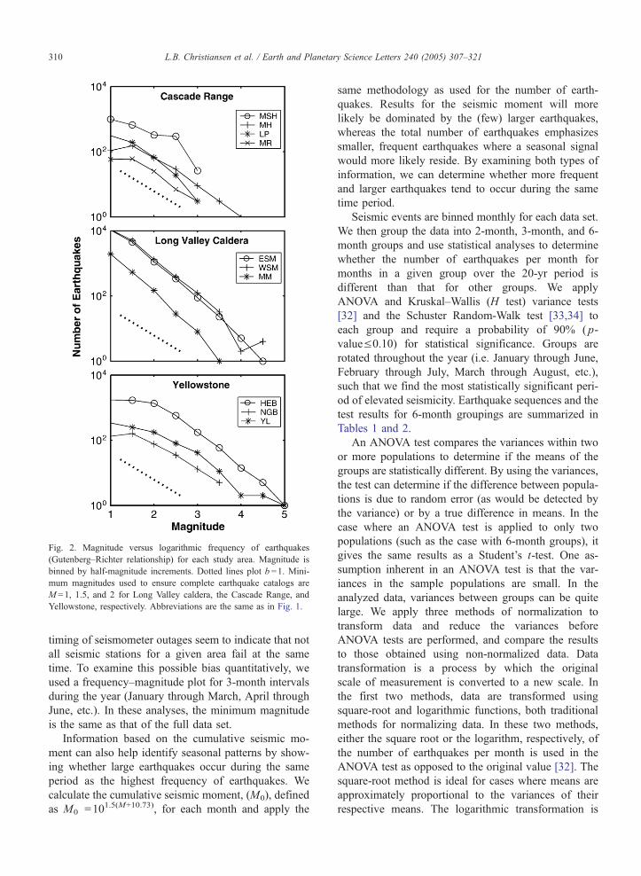
Fig. 2. Magnitude versus logarithmic frequency of earthquakes

(Gutenberg–Richter relationship) for each study area. Magnitude is

binned by half-magnitude increments. Dotted lines plot b =1. Mini-

mum magnitudes used to ensure complete earthquake catalogs are

M =1, 1.5, and 2 for Long Valley caldera, the Cascade Range, and

Yellowstone, respectively. Abbreviations are the same as in Fig. 1.


timing of seismometer outages seem to indicate that not

all seismic stations for a given area fail at the same

time. To examine this possible bias quantitatively, we

used a frequency–magnitude plot for 3-month intervals

during the year (January through March, April through

June, etc.). In these analyses, the minimum magnitude

is the same as that of the full data set.

Information based on the cumulative seismic mo-

ment can also help identify seasonal patterns by show-

ing whether large earthquakes occur during the same

period as the highest frequency of earthquakes. We

calculate the cumulative seismic moment, (M0), defined

as M0 =101.5(M+10.73), for each month and apply the

same methodology as used for the number of earth-

quakes. Results for the seismic moment will more

likely be dominated by the (few) larger earthquakes,

whereas the total number of earthquakes emphasizes

smaller, frequent earthquakes where a seasonal signal

would more likely reside. By examining both types of

information, we can determine whether more frequent

and larger earthquakes tend to occur during the same

time period.

Seismic events are binned monthly for each data set.

We then group the data into 2-month, 3-month, and 6-

month groups and use statistical analyses to determine

whether the number of earthquakes per month for

months in a given group over the 20-yr period is

different than that for other groups. We apply

ANOVA and Kruskal–Wallis (H test) variance tests

[32] and the Schuster Random-Walk test [33,34] to

each group and require a probability of 90% ( p-

valueV0.10) for statistical significance. Groups are

rotated throughout the year (i.e. January through June,

February through July, March through August, etc.),

such that we find the most statistically significant peri-

od of elevated seismicity. Earthquake sequences and the

test results for 6-month groupings are summarized in

Tables 1 and 2.

An ANOVA test compares the variances within two

or more populations to determine if the means of the

groups are statistically different. By using the variances,

the test can determine if the difference between popula-

tions is due to random error (as would be detected by

the variance) or by a true difference in means. In the

case where an ANOVA test is applied to only two

populations (such as the case with 6-month groups), it

gives the same results as a Student’s t-test. One as-

sumption inherent in an ANOVA test is that the var-

iances in the sample populations are small. In the

analyzed data, variances between groups can be quite

large. We apply three methods of normalization to

transform data and reduce the variances before

ANOVA tests are performed, and compare the results

to those obtained using non-normalized data. Data

transformation is a process by which the original

scale of measurement is converted to a new scale. In

the first two methods, data are transformed using

square-root and logarithmic functions, both traditional

methods for normalizing data. In these two methods,

either the square root or the logarithm, respectively, of

the number of earthquakes per month is used in the

ANOVA test as opposed to the original value [32]. The

square-root method is ideal for cases where means are

approximately proportional to the variances of their

respective means. The logarithmic transformation is

Table 2

Results for regions that show seasonality in three out of five tests

(excluding Schuster tests) for 2- and 3-month binning, for cumulative

seismic moment (6-month binning), and for the top 3 km of the crust

only

Location A Asqrt Alog Ayr K–W

Full data set

3-month

Yellowstone Lake 0.04 0.02 0.11 0.06 0.11

2-month

Mt. St. Helens 0.30 0.31 0.04 0.01 0.04


Cumulative Seismic

Moment (6-month)

Mt. St. Helens 0.10 0.05 0.07 0.08 0.08

Eastern south moat 0.04 0.02 0.07 0.02 0.18

Mammoth Mountain 0.16 0.07 0.04 0.04 0.005


Top 3 km

6-month

Mt. St. Helens 0.19 0.06 0.04 0.01 0.05



Hebgen L./Madison V. 0.04 0.06 0.09 0.03 0.08


3-month





2-month




Abbreviations are the same as in Table 1. Significant values are in

bold.

Table 1

Results of statistical analyses

Location Number of earthquakes A Asqrt Alog Ayr K–W Sch. Seasonal ?

Cascades

Mt. St. Helens 1306 0.20 0.05 0.04 0.02 0.03 0.27 UMt. Hood 187 0.30 0.49 0.32 0.33 0.32 0.02

Lassen Peak 154 0.22 0.25 0.20 0.10 0.25 0.15

Mt. Rainier 63 0.21 0.19 0.13 0.22 0.13 0.07

Long Valley

Eastern south moat 16558 0.06 0.10 0.17 0.05 0.18 b0.001 UWestern south moat 17768 0.12 0.23 0.25 0.004 0.28 b0.001

Mammoth Mountain 2650 0.05 0.03 0.03 0.002 0.007 b0.001 UYellowstone

Hebgen L./Madison V. 1967 0.15 0.32 0.60 0.17 0.69 b0.001

Norris Geyser Basin 161 0.28 0.28 0.21 0.37 0.18 0.04

Yellowstone Lake 497 0.01 0.003 0.02 0.01 0.02 0.20 U

A=ANOVA, Asqrt=ANOVA with a square-root normalization, Alog=ANOVA with a logarithmic normalization, Ayr=ANOVA with yearly

normalization, K–W=Kruskal–Wallis, and Sch.=Schuster Random Walk. Significant values are in bold. Results are for 6-month binning. Regions

where data show convincing evidence for seasonality are identified in the last column.


appropriate if means are proportional to the range or

standard deviation of respective means. The third meth-

od for normalizing data specifically addresses interan-

nual variability in the amount of seismicity, such as

might be associated with magmatically or tectonically

driven seismicity. For each year analyzed, we divide

the number of earthquakes for each month by the

maximum monthly total for that year, so that the

monthly number of earthquakes may vary between 0

and 1. Each year is normalized independently. With

this normalization method, each year has the same

weight as other years in the analysis. Thus, a year

with many earthquakes does not dominate the pattern.

Because a large number of measurements are needed

before any definite conclusion can be made about the

most appropriate transformation, we compare all three

methods to ensure that the transformations are not

altering the end results.

The Kruskal–Wallis test is a rank-sum method that

determines if random samples come from identical

populations. By ranking the data instead of using the

raw values, assumptions about the distributions of the

populations are unnecessary. Therefore, we do not need

to transform the data to use this test.

The Schuster Random Walk test has been applied in

previous studies to assess periodic signals in seismicity

(e.g. [13,14,35]). In this test, each seismic event is

given a unit length and assigned an angle from 08 to

3608, depending on the day of the year (January 1 is

given an angle of 08). Each vector is plotted sequen-

tially, tail to head, to create a random walk line depict-

ing the timing of events. As the distance of the random


walk line from the origin increases, the probability for a

non-uniformly distributed population increases. The

path of the random walk line shows the sequential

timing of earthquake events throughout the course of

time series. A randomly distributed population will

produce an average walkout length with a radius of

R ¼ 0:5ffiffiffiffiffiffiffipN

pfrom the origin. The Schuster test pro-

vides an expression for determining the probability,

Prw, that a randomly distributed population would

exceed R, based on the distance of the random

walk, D, for a given number of events, N:

Prw ¼ exp � D2=N� �

: ð2Þ

If the end distance of the random walk exceeds a

certain probability, the null hypothesis of random

event phases can be rejected and the population may

contain a nonrandom component [33,34].

In many cases, close examination of Schuster test

results reveals that one or more years dominate the

random walk pattern, due to elevated levels of seismic-

ity as compared to more typical years. The high-seis-

micity periods, likely caused by either magma

intrusions or tectonic activity and unrelated to seasonal

patterns, are classified as swarm periods. We develop a

method to remove these periods from the catalog for

each location (Appendix A). The seismic moment,

which has both an angular vector (determined by the

date) and a magnitude (determined by the moment),

cannot be examined using a Schuster test. Another

drawback of this test is that it may tend to overestimate

the significance of the results [36]. Under some circum-

stances, it can also underestimate seasonality: as years

of data are removed during deswarming, the length of

the time series is reduced, decreasing the statistical

significance.

4. Results

Data from 4 of the 10 regions show a statistically

significant increase in monthly seismicity during a

given time of the year, hereafter referred to as season-

ality (Table 1). Results from the different statistical tests

did not agree in all cases, and we consider statistical

significance of z90% in four of the six tests to be

convincing evidence of seasonality. When data were

grouped by 2- or 3-month groups, a statistically signif-

icant period of increased seismicity was not detected in

any of the regions. However, at Yellowstone Lake, 2-

and 3-month groups display seasonality in three of the

six tests. In data from Mt. St. Helens, three of six tests

indicate seasonality in 2-month groups, but not 3-month

groups. The remainder of the discussion will refer to 6-

month groups unless otherwise stated. Test results

based on the cumulative monthly seismic moment

show similar results to those that examined the number

of earthquakes (Table 2).

Certain statistical tests tend to overestimate the like-

liness of seasonality. In particular, Schuster tests results

indicate a non-random component in the distribution of

earthquakes in 7 of the 10 regions, often in conflict with

all other tests. In addition, data from some regions

which prove to have a seasonal component based on

ANOVA or Kruskal–Wallis tests are not identified

using the Schuster test methodology. For two locations,

yearly normalization appears to overstate the signifi-

cance of seasonality as compared to the other tests.

Other methods for data transformation, and the non-

normalized data, all generally provided similar results,

although sample population variances were high in the

non-normalized and square-root transformation meth-

ods. We conclude that the best approach to assessing

seasonality is to apply several statistical tests side by

side in order to generate robust, plausible results.

In the Cascade Range, Mt. St. Helens is the only

volcanic area where data show convincing evidence for

seasonal seismicity. Four of the six statistical tests

(ANOVA with square root, logarithmic, and yearly

normalization, and the Kruskal–Wallis test) indicate

elevated seismicity during May through November

(Table 1; Fig. 3). p-Values range from 0.02 in the

ANOVA test with yearly normalization to 0.05 in the

ANOVA test with a square root transformation. The

ANOVA test without normalization and the Schuster

test do not indicate any trends in the timing of earth-

quakes. The cumulative seismic moment at Mt. St.

Helens increases from May through December in all

five statistical tests ( p-values ranging from 0.05 to

0.10), consistent with the results based on the number

of earthquakes. In the other three volcanic areas in the

Cascades, statistical significance was met in only one of

the six tests, leading us to believe that there is no

detectable seasonal pattern to earthquake timing and

magnitude. In contrast to an earlier study exploring

seasonality at Mt. Hood [17], our statistical analyses

do not indicate seasonality there. This difference may

be due to their data preprocessing and relatively short

time series for use in power spectra, while we focus on

a variety of standard statistical techniques of unpro-

cessed data with comparison to normalized time series.

We calculate power spectra of unprocessed data from

areas with seasonal seismicity (discussed later) for

comparison to other studies.

In LVC, data from both Mammoth Mountain and the

eastern south moat region show seasonal modulation of

Fig. 3. Timing for elevated seismicity for each region that has statistically significant seasonality. For the Hebgen Lake/Madison Valley region, we

use data from only the upper 3 km of the crust. The timing varies depending on the statistical test. The bold line represents the time interval that

coincides in all statistical tests, whereas the grey dashed line shows the possible extent of increased seismicity based on individual tests. Shaded

grey areas show timing of peak snow water equivalent (SWE), peak lake level at Yellowstone Lake (YL), and peak water table levels based on well

data from Long Valley caldera. Thicker lines for Mammoth Mountain, Hebgen Lake/Madison Valley, and Yellowstone Lake show timing for 2- and

3-month periods of elevated seismicity in the top 3 km of the crust only.


seismicity. At Mammoth Mountain, all six statistical

tests indicate significance, with p-values ranging from

b0.001 (Schuster) to 0.05 (ANOVA). Increased seis-

micity occurs from approximately May through De-

cember, depending on the test. Seasonality in the

cumulative seismic moment is significant in four of

the five analyses ( p-values range from 0.005 to 0.07,

excluding ANOVA). The timing of the elevated seismic

moment coincides with that of the elevated number of

earthquakes. In the eastern south moat, four of the six

tests indicate significant seasonality ( p-values range

from b0.001 to 0.10, excluding ANOVA with logarith-

mic normalization and Kruskal–Wallis). Seismicity is

elevated from October to May. The cumulative seismic

moment also increases during October through May,

with p-values ranging from 0.02 to 0.07, excluding

Kruskal–Wallis. In the western south moat, there is

evidence for non-randomly distributed seismicity in

the ANOVA test with yearly normalization and the

Schuster test. However, because the other tests do not

show indications of increased seismicity during a por-

tion of the year, we conclude that seasonal seismicity

cannot be confirmed in this region.

At Yellowstone, Yellowstone Lake has elevated seis-

micity from July through December. This period is

coincident with a period of lake level drop (http://

volcanoes.usgs.gov/yvo/LakeLevelData1990-2003.txt).

The increase in seismic activity is statistically signifi-

cant in five of the six tests ( p-values range from 0.003

to 0.02, excluding Schuster). Cumulative seismic mo-

ment is also elevated from July through December ( p-

values range from 0.03 to 0.08). Three statistical tests

(ANOVA and ANOVA with square root and yearly

normalization) show increased seismicity in both 2-

and 3-month groups. The 2-month period of increased

seismicity occurs between September and November,

depending on the test. The 3-month period of increased

seismicity occurs between September and December,

again depending on the test. The data from Norris

Geyser Basin and Hebgen Lake/Madison Valley display

seasonality in Schuster tests; however, the variance

tests indicate that events are randomly distributed.

Because of the possibility that seasonal variations in

seismicity may be induced by external forcing at the

ground surface [11,15,17,18], we use the same method-

ology to explore for seasonality in the upper 3 km of the

crust only. If less than 50 earthquakes occur in the upper

3 km of the crust (as in the case of Mt. Hood and Lassen

Peak), we use data from the upper 5 km. For each of the

regions where we found convincing evidence of season-

al seismicity for both deep and shallow earthquakes, we

found an equal or greater statistical significance in the

http:\\volcanoes.usgs.gov\yvo\LakeLevelData1990-2003.txt


shallower portions of the crust. For 2- and 3-month

groups, data from Mammoth Mountain, Hebgen Lake/

Madison Valley, and Yellowstone Lake display season-

ality (Table 2), indicating more focused periods of sea-

sonality. In addition, data from the shallow crust at

Hebgen Lake/Madison Valley suggest that seasonality

there is statistically significant ( p-values range from

0.03 to 0.09), with increased seismicity from June

through December, depending on the statistical test

(Table 2). Seasonality is also significant in 3-month

groups and in three out of five tests in 2-month groups.

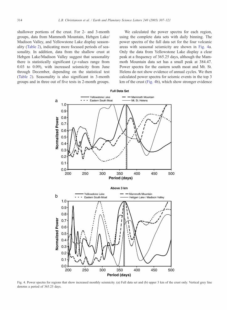
Fig. 4. Power spectra for regions that show increased monthly seismicity. (a

denotes a period of 365.25 days.

We calculated the power spectra for each region,

using the complete data sets with daily binning. The

power spectra of the full data set for the four volcanic

areas with seasonal seismicity are shown in Fig. 4a.

Only the data from Yellowstone Lake display a clear

peak at a frequency of 365.25 days, although the Mam-

moth Mountain data set has a small peak at 384.47.

Power spectra for the eastern south moat and Mt. St.

Helens do not show evidence of annual cycles. We then

calculated power spectra for seismic events in the top 3

km of the crust (Fig. 4b), which show stronger evidence

) Full data set and (b) upper 3 km of the crust only. Vertical grey line


for an annual period. The shallow data from both

Yellowstone Lake and Mammoth Mountain show clear-

ly defined peaks at 365.25 days, data from Hebgen

Lake/Madison Valley have a small peak at 384.47,

and data from the eastern south moat have a small

peak at 347.86 (Fig. 4b). Data from Mt. St. Helens

and the remaining volcanic areas show no distinguish-

able peaks and therefore are not represented in the

figure. Although 20 yr of data is relatively short for

calculating the power spectra of an annual period,

evidence for seasonality is apparent in four of the

regions.

5. Discussion

Significant annual periodicity in seismicity occurs in

4 of the 10 study regions (Table 1) and in 5 of 10 areas

if only the upper 3 km of the crust are examined (Table

2). The timing of increased seismicity varies between

locations and spans the whole year (Fig. 3). One region

has increased seismicity during winter, helping to reaf-

firm that the results are not significantly affected by

seismometer malfunctions during the winter months.

Because seasonality appears to be common, we explore

the possibility that external forces with annual frequen-

cies might trigger seismicity.

Triggered earthquakes can be induced by changing

the magnitude of stresses on faults. Earthquakes may be

induced by an increase in the effective stress normal to

a fault, a reduction in effective stress parallel to a fault,

or equal decreases in effective stress in all principal

directions. Mechanisms such as snow unloading, solid

earth tides, and barometric pressure variations increase/

decrease in stress in the vertical direction, whereas

groundwater recharge reduces effective stress in all

principal directions by increasing pore pressure. Previ-

ous studies of static stress change have concluded that,

in most cases, static stress changes of less than 10 kPa

are not sufficient to induce seismicity [37–39]. In lab-

oratory experiments, a strong correlation between peri-

odic stress and failure occurs at amplitudes of 50 to 100

kPa [40].

5.1. Snow unloading

Heki [15] suggested that unloading of snow on the

western flanks of the Backbone Range in Japan triggers

seasonal (spring–summer) earthquakes with M N7. Re-

moval of the snow load (up to 10 kPa) in the spring

may cause failure in shallow faults and initiate earth-

quakes. The vertical stress change at the surface during

snow unloading is equal in magnitude and opposite in

sign to the pressure created by the maximum snow load

during mid-March through mid-May. Unloading should

reduce vertical stress and unclamp normal faults, but

should be less effective in triggering seismic activity on

strike-slip faults. Most of the volcanic areas examined

here are dominated by normal faults, but oblique and

strike-slip faults are also present [21,29,41–43]. The

faults at Mt. St. Helens are primarily strike-slip, as

inferred from focal mechanisms [21].

In the Cascades, LVC, and Yellowstone, seismicity

peaks at times ranging from less than 1 month to 6

months after timing of maximum snow load (Fig. 3).

Stresses produced by the surface load propagate to

seismogenic depths essentially instantaneously. The

lag time between the onset of snow melt (unloading)

and increased seismicity is not consistent with the crust

behaving elastically, and may reflect a number of pro-

cesses including: (1) variability in the response of crack

growth to stress in the fault zone [35]; (2) the ability of

fluids to reach crack tips and thus cause crack propa-

gation [44,45]; (3) viscoelastic effects of the crust,

affecting the fracture propagation [46]; and (4) longer

nucleation time required for larger earthquakes, where-

as smaller earthquakes may be modulated by shorter-

term disturbances such as daily tides [15].

The average snow water equivalent (SWE) for April

1, historically the period of maximum snow accumula-

tion, ranges from 0.5 to 1 m in the volcanic regions that

have seasonal seismicity (http://cdec.water.ca.gov/snow/

current/snow/; http://www.wcc.nrcs.usda.gov/snotel/).

These loads result in a near-surface stress of 5–10

kPa. There is no snow load data in the eastern south

moat so we use values at Mammoth Mountain as an

approximation.

The total stress at the surface (e.g. the snow load),

rt, is borne by both the pore fluid and the rock matrix,

reducing the effective stress at seismogenic depths. The

portion carried by pore fluid is determined by a tidal

efficiency factor, a, which is dependent on bulk com-

pressibility [47]:

a ¼ bb

bb þ /bw

ð3Þ

where bb is bulk compressibility of the porous medium,

bw is the compressibility of water, and u is porosity.

Thus the effective stress, re, at depth is:

re ¼ rt � art: ð4Þ

Assuming that bulk compressibility of volcanic rock

ranges from 10�10 to 10�11 m2/N, a is calculated to be

0.2 to 0.5. Given that seismogenic depths range from 2

to 8 km in the volcanic regions that have seasonality,

http:\\cdec.water.ca.gov\snow\current\snow\

http:\\www.wcc.nrcs.usda.gov\snotel\


snow unloading may cause effective stress changes at

seismogenic depths in the range of 1–6 kPa (Table 3,

SWE load).

5.2. Groundwater recharge

Increases in pore fluid pressure caused by ground-

water recharge can trigger seismicity by reducing the

effective normal stress on faults. Unlike snow unload-

ing, this process affects all fault types (normal, reverse,

and strike-slip), because fluid pressure acts equally in

all directions, independent of the stress tensor (e.g.

[17]). Most groundwater recharge occurs during the

spring as snowmelt infiltrates. The time required for

the pressure pulse to diffuse from the surface to seis-

mogenic depths, which is dependent on the hydraulic

diffusivity and depth to the seismogenic zone, creates a

lag time between peak recharge and peak seismicity.

The calculated pressure increase at the surface

decays with depth, controlled by the hydraulic diffu-

sivity and the depth to the region where seismicity

occurs. Assuming that periodic groundwater recharge

is in fact the cause of seasonal seismicity, a bulk

hydraulic diffusivity can be calculated from the lag

time, t, between peak recharge and peak seismicity

[17]:

j ¼ Wz2

4pt2ð5Þ

where j is hydraulic diffusivity, z is the depth of

seismicity, and W =is the period of the seasonal near-

surface pore fluid pressure perturbation (1 yr).

To apply this equation, we assume that the medium

is saturated from the surface to the depth of seismicity,

and that the peak runoff time is June 1. The calculated

hydraulic diffusivities range from 1.0 to 13.5 m2/s in

the volcanic areas with seasonality (Table 3). These

calculated diffusivities are generally consistent with

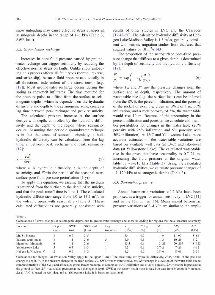
Table 3

Calculations of stress changes at seismogenic depths due to groundwater re

Location Depth

(km)

SWE

(m)

SWE load

(kPa)

Lag

(mont

Mt. St. Helens 3 0.9 2–5 1

Eastern south moat 8 1.1 2–6 5

Mammoth Mountain 6 1.1 2–6 1

Yellowstone Lake 5 0.5 1–3 1

Hebgen L./Madison V. 2 0.6 1–3 1

Calculations for Hebgen Lake/Madison Valley apply to the upper 3 km of

change at depth, PV, to the pressure change in the near-surface, P0, SWE=sn

complete melting of the SWE and associated groundwater recharge, assumin

the ground surface, DPV=calculated pressure at the seismogenic depth. SWE

Dh at LVC is based on well data and at Yellowstone Lake it is based on la

results of other studies in LVC and the Cascades

[17,48–50]. The calculated hydraulic diffusivity at Heb-

gen Lake/Madison Valley is 1.5 m2/s, generally consis-

tent with seismic migration studies from that area that

suggest values of 10 m2/s [43].

The proportion of the near-surface pore-fluid pres-

sure change that diffuses to a given depth is determined

by the depth of seismicity and the hydraulic diffusivity

[17]:

PV

P0

¼ exp � z

ffiffiffiffiffiffiffiffip

Wj

r ��ð6Þ

where P0 and PV are the pressure changes near the

surface and at depth, respectively. The amount of

water table rise (e.g. the surface load) can be inferred

from the SWE, the percent infiltration, and the porosity

of the rock. For example, given an SWE of 1 m, 50%

infiltration, and a rock porosity of 5%, the water table

would rise 10 m. Because of the uncertainty in the

percent infiltration and porosity, we calculate end-mem-

ber possibilities for changes in the water table (20%

porosity with 25% infiltration and 5% porosity with

50% infiltration). At LVC and Yellowstone Lake, more

accurate estimates of the water-table variations are

based on available well data (at LVC) and lake-level

data (at Yellowstone Lake). The calculated water-table

rise in the areas that have seasonality is 0.7–21 m,

increasing the fluid pressure at the original water

table by ~7–210 kPa (Table 3). Using the calculated

hydraulic diffusivities, we calculate pressure changes of

~1–120 kPa at seismogenic depths (Table 3).

5.3. Barometric pressure

Annual barometric variations of 2 kPa have been

proposed as a trigger for annual seismicity in LVC [11]

and in the Philippines [16]. Mean annual barometric

pressure variations of 2–4 kPa are similar to the ampli-

charge and snow unloading for regions that have seasonal seismicity

hs)

j(m2/s)

PV/P0

(%)

Dh

(m)

DP0

(kPa)

DPV(kPa)

3.4 0.7 1–9 11–90 8–64

1.0 0.1 1–3 10–29 1–2

13.5 0.6 3–21 29–206 18–123

9.3 0.6 0.7–2 7–20 4–12

1.5 0.6 0.8–6 8–61 5–36

the crust only. j =hydraulic diffusivity, PV/P0= ratio of the pressure

ow water equivalent, Dh =change in elevation of the water table due to

g 25–50% infiltration and 5–20% porosity, DP0=change in pressure at

at the eastern south moat is based on data from Mammoth Mountain.

ke level.

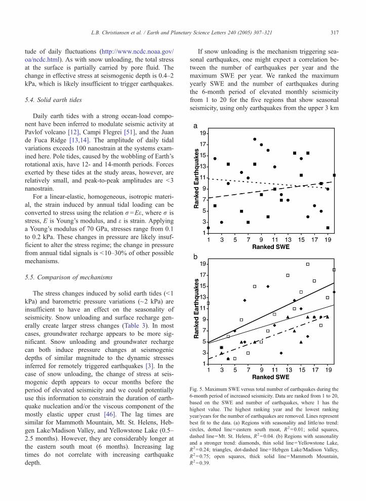
Fig. 5. Maximum SWE versus total number of earthquakes during the

6-month period of increased seismicity. Data are ranked from 1 to 20

based on the SWE and number of earthquakes, where 1 has the

highest value. The highest ranking year and the lowest ranking

year/years for the number of earthquakes are removed. Lines represen

best fit to the data. (a) Regions with seasonality and little/no trend

circles, dotted line=eastern south moat, R2=0.01; solid squares

dashed line=Mt. St. Helens, R2=0.04. (b) Regions with seasonality

and a stronger trend: diamonds, thin solid line=Yellowstone Lake

R2=0.24; triangles, dot-dashed line=Hebgen Lake/Madison Valley

R2=0.75; open squares, thick solid line=Mammoth Mountain

R2=0.39.


tude of daily fluctuations (http://www.ncdc.noaa.gov/

oa/ncdc.html). As with snow unloading, the total stress

at the surface is partially carried by pore fluid. The

change in effective stress at seismogenic depth is 0.4–2

kPa, which is likely insufficient to trigger earthquakes.

5.4. Solid earth tides

Daily earth tides with a strong ocean-load compo-

nent have been inferred to modulate seismic activity at

Pavlof volcano [12], Campi Flegrei [51], and the Juan

de Fuca Ridge [13,14]. The amplitude of daily tidal

variations exceeds 100 nanostrain at the systems exam-

ined here. Pole tides, caused by the wobbling of Earth’s

rotational axis, have 12- and 14-month periods. Forces

exerted by these tides at the study areas, however, are

relatively small, and peak-to-peak amplitudes are b3

nanostrain.

For a linear-elastic, homogeneous, isotropic materi-

al, the strain induced by annual tidal loading can be

converted to stress using the relation r =Ee, where r is

stress, E is Young’s modulus, and e is strain. Applying

a Young’s modulus of 70 GPa, stresses range from 0.1

to 0.2 kPa. These changes in pressure are likely insuf-

ficient to alter the stress regime; the change in pressure

from annual tidal signals is b10–30% of other possible

mechanisms.

5.5. Comparison of mechanisms

The stress changes induced by solid earth tides (b1

kPa) and barometric pressure variations (~2 kPa) are

insufficient to have an effect on the seasonality of

seismicity. Snow unloading and surface recharge gen-

erally create larger stress changes (Table 3). In most

cases, groundwater recharge appears to be more sig-

nificant. Snow unloading and groundwater recharge

can both induce pressure changes at seismogenic

depths of similar magnitude to the dynamic stresses

inferred for remotely triggered earthquakes [3]. In the

case of snow unloading, the change of stress at seis-

mogenic depth appears to occur months before the

period of elevated seismicity and we could potentially

use this information to constrain the duration of earth-

quake nucleation and/or the viscous component of the

mostly elastic upper crust [46]. The lag times are

similar for Mammoth Mountain, Mt. St. Helens, Heb-

gen Lake/Madison Valley, and Yellowstone Lake (0.5–

2.5 months). However, they are considerably longer at

the eastern south moat (6 months). Increasing lag

times do not correlate with increasing earthquake

depth.

If snow unloading is the mechanism triggering sea-

sonal earthquakes, one might expect a correlation be-

tween the number of earthquakes per year and the

maximum SWE per year. We ranked the maximum

yearly SWE and the number of earthquakes during

the 6-month period of elevated monthly seismicity

from 1 to 20 for the five regions that show seasonal

seismicity, using only earthquakes from the upper 3 km

,

t

:

,

,

,

,

http:\\www.ncdc.noaa.gov\oa\ncdc.html


of the crust for Hebgen Lake/Madison Valley. The year

with the greatest number of earthquakes (ranked 1) was

removed from the data set, because in most cases the

number of earthquakes in this year was an order of

magnitude larger than in the rest of the years, and likely

related to magmatic or tectonic activity as opposed to

external forcing. Similarly, we removed the lowest

ranking year(s) and years with V1 earthquake because

years with very low seismicity were indistinguishable.

Although the data show considerable scatter, three of

the five regions show a moderate correlation between

years with increased seismicity and years with greater

snow load (Fig. 5).

Groundwater recharge causes calculated stress

increases at the depth of seismicity that are typically

larger than those induced by snow unloading (Table 3).

The interannual variability in groundwater recharge is

likely correlated with SWE and could also explain the

moderate correlation between number of earthquakes

and the magnitude of SWE (Fig. 5). Further, diffusion

of pore-fluid pressure changes can most readily explain

the lag time between groundwater recharge and the onset

of seismicity. Hydraulic diffusivities calculated from the

lag times generally fall within the large range of values

determined empirically and theoretically. Longer lag

times, like those observed at the eastern south moat at

LVC, imply low hydraulic diffusivity and very small

pressure increases. In some cases, such as in the Cascade

Range, the water table can be far below the land surface

[52]. In such instances, water would first have to reach

the water table before pore pressure diffusion can begin.

Additionally, if the pore pressure gradient is sufficiently

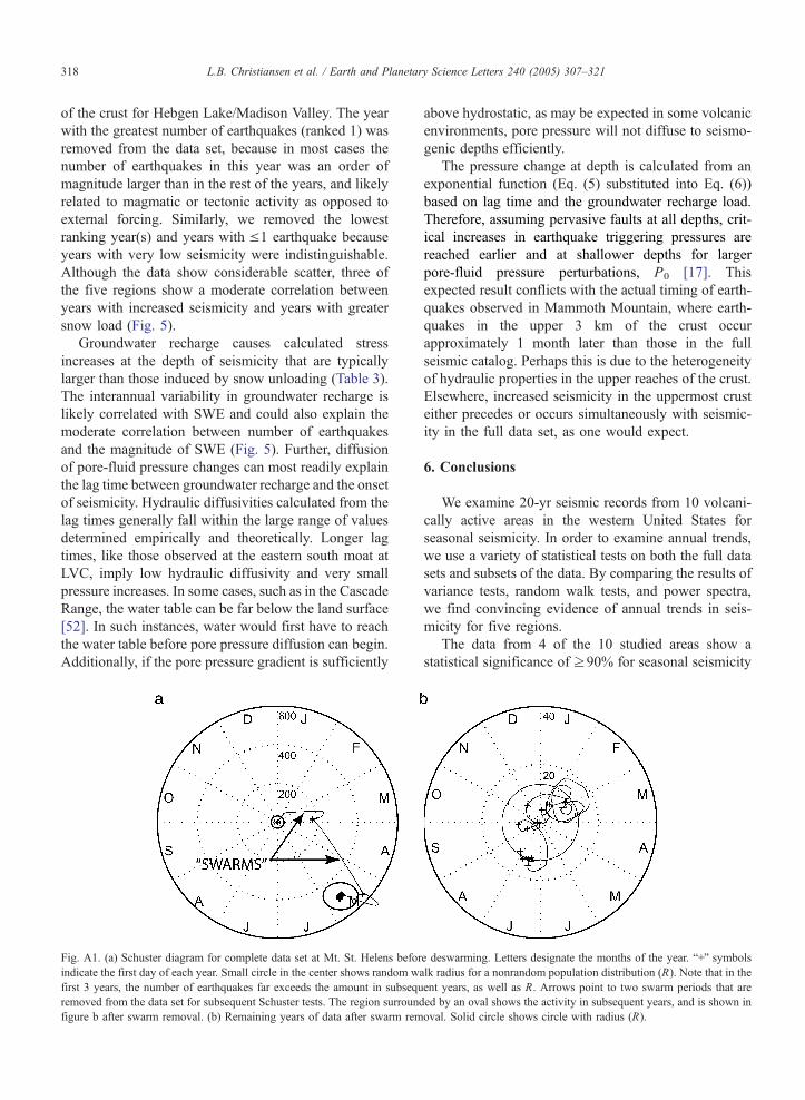
Fig. A1. (a) Schuster diagram for complete data set at Mt. St. Helens befor

indicate the first day of each year. Small circle in the center shows random w

first 3 years, the number of earthquakes far exceeds the amount in subsequ

removed from the data set for subsequent Schuster tests. The region surround

figure b after swarm removal. (b) Remaining years of data after swarm rem

above hydrostatic, as may be expected in some volcanic

environments, pore pressure will not diffuse to seismo-

genic depths efficiently.

The pressure change at depth is calculated from an

exponential function (Eq. (5) substituted into Eq. (6))

based on lag time and the groundwater recharge load.

Therefore, assuming pervasive faults at all depths, crit-

ical increases in earthquake triggering pressures are

reached earlier and at shallower depths for larger

pore-fluid pressure perturbations, P0 [17]. This

expected result conflicts with the actual timing of earth-

quakes observed in Mammoth Mountain, where earth-

quakes in the upper 3 km of the crust occur

approximately 1 month later than those in the full

seismic catalog. Perhaps this is due to the heterogeneity

of hydraulic properties in the upper reaches of the crust.

Elsewhere, increased seismicity in the uppermost crust

either precedes or occurs simultaneously with seismic-

ity in the full data set, as one would expect.

6. Conclusions

We examine 20-yr seismic records from 10 volcani-

cally active areas in the western United States for

seasonal seismicity. In order to examine annual trends,

we use a variety of statistical tests on both the full data

sets and subsets of the data. By comparing the results of

variance tests, random walk tests, and power spectra,

we find convincing evidence of annual trends in seis-

micity for five regions.

The data from 4 of the 10 studied areas show a

statistical significance of z90% for seasonal seismicity

e deswarming. Letters designate the months of the year. b+Q symbols

alk radius for a nonrandom population distribution (R). Note that in the

ent years, as well as R. Arrows point to two swarm periods that are

ed by an oval shows the activity in subsequent years, and is shown in

oval. Solid circle shows circle with radius (R).


and data from 5 areas indicate a significance of z90%

for seasonal seismicity in the upper 3 km of the crust.

Four of those regions have pronounced annual peaks in

power spectra for the upper 3 km of crust. In four of the

five regions, seismicity peaks during the summer

months, from approximately June through December.

In the other region, increased seismicity occurs later in

the year, from approximately November through April.

In all cases, the cumulative seismic moment also

increases during these periods.

We explored four possible triggering mechanisms

for the observed seasonal seismicity. Both solid earth

tides and barometric pressure variations cause changes

in static stress of V2 kPa, likely insufficient to trigger

seismicity. The static stress changes induced by snow

unloading are as great as 5–6 kPa at Mt. St. Helens and

LVC and somewhat lower at Yellowstone (1–3 kPa).

Groundwater recharge may increase pore pressure at

seismogenic depths by up to 120 kPa. Plausible values

of hydraulic diffusivity, ranging from 1 to 13 m2/s, are

obtained from the apparent lag time between peak

recharge and peak seismicity. For most regions showing

seasonal seismicity, there is also a correlation between

the magnitude of the SWE and the number of earth-

quakes in that year.

Acknowledgements

The authors would like to thank Nick Beeler, Dave

Hill, Malcolm Johnston, Paul Reasenberg, Evelyn

Roeloffs, and two anonymous reviewers for their con-

structive comments during the writing of this paper.

We would also like to thank the National Research

Council for funding for L.B. Christiansen. Funding for

this research came from the USGS Volcano Hazards

Program.

Appendix A

Schuster tests often reveal that one or more years of

seismic data dominate the random walk pattern, indi-

cating elevated seismic activity as compared to more

typical years (Fig. A1a). The high-seismicity periods,

likely caused by either magma intrusions or tectonic

activity and unrelated to seasonal patterns, are classified

as swarm periods. We define a swarm period as any

single year in which the Schuster Random Walk

exceeds the average walkout length (R). This length,

R, is dependent on the number of events in the time

series; as the length of the time series increases, R

increases, which classifies less seismic sequences as

earthquake swarms. However, with a longer time series,

each year has a smaller effect on the overall distribution

and therefore would not cause as severe a bias to the

analysis results. In order to maintain a continuous time

series, we remove a complete year of data surrounding

the swarm period for the Schuster test analyses only.

We determine the start and end dates of the excised year

by establishing the day on which most seismic activity

occurs and then removing half a year of data before and

after that day. We use full data sets in determining

minimum magnitude cutoffs and swarm periods. We

then retest the reduced data sets using Schuster tests to

quantify annual seasonal seismicity (Fig. A1b). The

south moat of LVC experiences swarm sequences al-

most yearly. Other areas also exhibit relatively frequent,

non-seasonal swarm sequences.

References

[1] D.P. Hill, P.A. Reasenberg, A.J. Michael, W.J. Arabasz, G.C.

Beroza, D.S. Brumbaugh, J.N. Brune, R. Castro, S.D. Davis,

D.M. dePolo, W.L. Ellsworth, J.S. Gomberg, S.C. Harmsen, L.

House, S.M. Jackson, M.J.S. Johnston, L.M. Jones, R. Keller,

S.D. Malone, L. Munguia, S. Nava, J.C. Pechmann, A.R. San-

ford, R.W. Simpson, R.B. Smith, M.A. Stark, M.C. Stickney, A.

Vidal, S.R. Walter, V. Wong, J.E. Zollweg, Seismicity remotely

triggered by the magnitude 7.3 Landers, California, earthquake,

Science 260 (1993) 1617–1623.

[2] S. Husen, R. Taylor, R.B. Smith, H. Healser, Changes in geyser

eruption behavior and remotely triggered seismicity in Yellow-

stone National Park produced by the 2002 M 7.9 Denali Fault

earthquake, Alaska, Geology 32 (2004) 537–540.

[3] S.G. Prejean, D.P. Hill, E.E. Brodsky, S.E. Hough, M.J.S.

Johnston, S.D. Malone, D.H. Oppenheimer, A.M. Pitt, K.B.

Richards-Dinger, Remotely triggered seismicity on the United

States west coast following the Mw 7.9 Denali fault earthquake,

Bull. Seismol. Soc. Am. 94 (2004) S348–S359.

[4] E.E. Brodsky, B. Sturtevant, H. Kanamori, Earthquakes, volca-

noes, and rectified diffusion, J. Geophys. Res. 103 (1998)

23827–23838.

[5] J. Gomberg, N.M. Beeler, M.L. Blanpied, P. Bodin, Earthquake

triggering by transient and static deformation, J. Geophys. Res.

103 (1998) 24411–424426.

[6] D.P. Hill, F. Pollitz, C. Newhall, Earthquake–volcano interac-

tions, Phys. Today 55 (2002) 41–47.

[7] A.T. Linde, I.S. Sacks, M.J.S. Johnston, D.P. Hill, R.G. Bilham,

Increased pressure from rising bubbles as a mechanism for

remotely triggered seismicity, Nature 371 (1994) 408–410.

[8] E.E. Brodsky, E. Roeloffs, D. Woodcock, I. Gall, M. Manga, A

mechanism for sustained groundwater pressure changes induced

by distant earthquakes, J. Geophys. Res. 108 (2003), doi:10.1029/

2002JB002321.

[9] D.P. Hill, J.O. Langbein, S. Prejean, Relations between seismic-

ity and deformation during unrest in Long Valley Caldera,

California, from 1995 through 1999, J. Volcanol. Geotherm.

Res. 127 (2003) 175–193.

[10] M.J.S. Johnston, D.P. Hill, A.T. Linde, J. Langbein, R. Bilham,

Transient deformation during triggered seismicity from the June

28, 1992, Mw =7.3 Landers earthquake at Long Valley volcanic

caldera California, Bull. Seismol. Soc. Am. 85 (1995) 787–795.


[11] S.S. Gao, P.G. Silver, A.T. Linde, I.S. Sacks, Annual modulation

of triggered seismicity following the 1992 Landers earthquake in

California, Nature 406 (2000) 500–504.

[12] S.R. McNutt, R.J. Beavan, Volcanic earthquakes at Pavlof

volcano correlated with solid earth tide, Nature 294 (1981)

615–618.

[13] M. Tolstoy, F.L. Vernon, J.A. Orcutt, F.K. Wyatt, Breathing of

the seafloor; tidal correlations of seismicity at Axial Volcano,

Geology 30 (2002) 503–506.

[14] W.S.D. Wilcock, Tidal triggering of microearthquakes on

the Juan de Fuca Ridge, Geophys. Res. Lett. 28 (2001)

3999–4002.

[15] K. Heki, Snow load and seasonal variation of earthquake

occurrence in Japan, Earth Planet. Sci. Lett. 207 (2003)

159–164.

[16] M. Ohtake, H. Nakahara, Seasonality of great earthquake occur-

rence at the northwestern margin of the Philippine Sea Plate,

Pure Appl. Geophys. 155 (1999) 689–700.

[17] M.O. Saar, M. Manga, Seismicity induced by seasonal ground-

water recharge at Mt. Hood, Oregon, Earth Planet. Sci. Lett. 214

(2003) 605–618.

[18] L.W. Wolf, C.A. Rowe, R.B. Horner, Periodic seismicity near

Mt. Ogden on the Alaska–British Columbia border; a case for

hydrologically triggered earthquakes? Bull. Seismol. Soc. Am.

87 (1997) 1473–1483.

[19] J.B. Adams, M.E. Mann, C.M. Ammann, Proxy evidence for an

El Nino-like response to volcanic forcing, Nature 426 (2003)

274–278.

[20] B.G. Mason, D.M. Pyle, W.B. Dade, T. Jupp, Seasonality of

volcanic eruptions, J. Geophys. Res. 109 (2004), doi:10.1029/

2002JB002293.

[21] S.C. Moran, Seismicity at Mount St. Helens, 1987–1992: evi-

dence for repressuring of an active magmatic system, J. Geo-

phys. Res. 99 (1994) 4341–4354.

[22] S.C. Moran, J.M. Lees, S.D. Malone, P wave crustal velocity

structure in the greater Mt. Rainier area from local earthquake

tomography, J. Geophys. Res. 104 (1999) 10775–710786.

[23] R.D. Norris, C.S. Weaver, K.L. Meagher, A. Qamarer, R.J.

Blakely, Earthquake swarms at Mount Hood; relation to geolog-

ic structure, Seismol. Res. Lett. 70 (1999) 218.

[24] S.R. Walter, Ten years of earthquakes at Lassen Peak, Mount

Shasta, and Medicine Lake volcanoes, Northern California;

1981–1990, Seismol. Res. Lett. 62 (1991) 25.

[25] D.P. Hill, R.A. Bailey, A.S. Ryall, Active tectonic and magmatic

processes beneath Long Valley Caldera, eastern California; an

overview, J. Geophys. Res. 90 (1985) 11111–111120.

[26] R.A. Bailey, G.B. Dalrymple, M.A. Lanphere, Volcanism, struc-

ture, and geochronology of Long Valley Caldera, Mono County,

California, J. Geophys. Res. 81 (1976) 725–744.

[27] M.L. Sorey, Evolution and present state of the hydrothermal

system in Long Valley Caldera, J. Geophys. Res. 90 (1985)

11219–211228.

[28] R.L. Christiansen, The Quaternary and Pliocene Yellowstone

Plateau volcanic field of Wyoming, Idaho, and Montana, U. S.

Geol. Surv. Prof. Pap. (2001) G1–G145.

[29] G.P. Waite, R.B. Smith, Seismotectonics and stress field of the

Yellowstone volcanic plateau from earthquake first-motions and

other indicators, J. Geophys. Res. 109 (2004), doi:10.1029/

2003JB002675.

[30] D.I. Doser, Source parameters and faulting processes of the 1959

Hebgen Lake, Montana, earthquake sequence, J. Geophys. Res.

90 (1985) 4537–4555.

[31] L.A. Morgan, W.C. Shanks III, D.A. Lovalvo, S.Y. Johnson,

W.J. Stephenson, K.L. Pierce, S.S. Harlan, C.A. Finn, G. Lee,

M. Webring, B. Schulze, J. Duehn, R.E. Sweeney, L.S. Balis-

trieri, Exploration and discovery in Yellowstone Lake; results

from high-resolution sonar imaging, seismic reflection profiling,

and submersible studies, J. Volcanol. Geotherm. Res. 122 (2003)

221–242.

[32] W.J. Dixon, J.F.J. Massey, Introduction to Statistical Analysis,

McGraw-Hill Book Company, New York, 1983. 678 pp.

[33] A. Schuster, On lunar and solar periodicities of earthquakes,

Proc. R. Soc. Lond. 61 (1897) 455–465.

[34] P.A. Rydelek, L. Hass, On estimating the amount of blasts in

seismic catalogs with Schuster’s Method, Bull. Seismol. Soc.

Am. 84 (1994) 1256–1259.

[35] N.M. Beeler, D.A. Lockner, Why earthquakes correlate weakly

with the solid Earth tides: effects of periodic stress on the rate

and probability of earthquake occurrence, J. Geophys. Res. 108

(2003) , doi:10.1029/2001JB001518.

[36] E.S. Cochran, J.E. Vidale, S. Tanaka, Earth tides can

trigger shallow thrust fault earthquakes, Science 306 (2004)

1164–1166.

[37] J.L. Hardebeck, J.J. Nazareth, E. Hauksson, The static stress

change triggering model; constraints from two Southern Cali-

fornia aftershock sequences, J. Geophys. Res. 103 (1998)

24427–424437.

[38] P.A. Reasenberg, R.W. Simpson, Response of regional seismic-

ity to the static stress change produced by the Loma Prieta

earthquake, Science 255 (1992) 1687–1690.

[39] R.W. Simpson, P.A. Reasenberg, Earthquake-induced static-

stress changes on Central California faults, U. S. Geol. Surv.

Prof. Pap. (1994) F55–F89.

[40] D.A. Lockner, N.M. Beeler, Premonitory slip and tidal trigger-

ing of earthquakes, J. Geophys. Res., B, Solid Earth Planets 104

(1999) 20133–120151.

[41] J. Jones, S.D. Malone, Constraints on Mt. Hood earthquake

swarms from cross-correlation and joint hypocenter determina-

tion, Seismol. Res. Lett. 73 (2002) 253.

[42] L.J.P. Muffler, M.A. Clynne, D.E. Champion, Late Quaternary

normal faulting of the Hat Creek Basalt, northern California,

Geol. Soc. Amer. Bull. 106 (1994) 195–200.

[43] G.P. Waite, R.B. Smith, Seismic evidence for fluid migration

accompanying subsidence of the Yellowstone Caldera, J. Geo-

phys. Res. 107 (9) (2002) 13.

[44] R.J. Martin III, Time-dependent crack growth in quartz and its

application to the creep of rocks, J. Geophys. Res. 77 (1972)

1406–1419.

[45] R.J. Martin III, W.B. Durham, Mechanisms of crack growth in

quartz, J. Geophys. Res. 80 (1975) 4837–4844.

[46] A.M. Jellinek, M. Manga, M.O. Saar, Did melting glaciers cause

volcanic eruptions in eastern California? Probing the mechanics

of dike formation, J. Geophys. Res. (2004), doi:10.1029/

2004JB002978.

[47] P.A. Domenico, F.W. Schwatrz, Physical and Chemical

Hydrogeology, John Wiley & Sons, Inc., New York, 1990.

506 pp.

[48] E. Roeloffs, M. Sneed, D.L. Galloway, M.L. Sorey, C.D. Farrar,

J.F. Howle, J. Huges, Water-level changes induced by local and

distant earthquakes at Long Valley caldera, California, J. Volca-

nol. Geotherm. Res. 127 (2003) 269–303.

[49] S.A. Rojstaczer, Intermediate period response of water levels in

wells to crustal strain; sensitivity and noise level, J. Geophys.

Res. 93 (1988) 13619–613634.


[50] M.O. Saar, M. Manga, Depth dependence of permeability in the

Oregon Cascades inferred from hydrogeologic, thermal, seismic,

and magmatic modeling constraints, J. Geophys. Res. 109

(2004), doi:10.1029/2003JB002855.

[51] P.A. Rydelek, I.S. Sacks, R. Scarpa, On tidal triggering of

earthquakes at Campi Flegrei, Italy, Geophys. J. Int. 109

(1992) 125–137.

[52] S. Hurwitz, K.L. Kipp, M.E. Reid, S.E. Ingebritsen, Groundwa-

ter flow, heat transport, and water-table position within volcanic

edifices: implications for volcanic processes in the Cascade

Range, J. Geophys. Res. (2003), doi:10.1029/2003JB002565.

Download - Seasonal seismicity at western United States volcanic centers · Seasonal seismicity at western United States volcanic centers L.B. Christiansen a,*, ... removal of the snow load,

Top Related