dp2006/03 asmallnewkeynesianmodelofthenew … · dp2006/03 asmallnewkeynesianmodelofthenew...
TRANSCRIPT

DP2006/03
A Small New Keynesian Model of the NewZealand Economy
Philip Liu
May 2006
JEL classification: C15, C51, E12, E17
www.rbnz.govt.nz/research/discusspapers/
Discussion Paper Series

DP2006/03
A Small New Keynesian Model of the New Zealand
Economy∗
Philip Liu†
Abstract
This paper investigate whether a small open economy DSGE-based New Key-nesian model can provide a reasonable description of key features of the NewZealand economy, in particular the transmission mechanism of monetary pol-icy. The main objective is to design a simple, compact, and transparent toolfor basic policy simulations. The structure of the model is largely motivatedby recent developments in the area of DSGE modelling. Combining priorinformation and the historical data using Bayesian simulation techniques, wearrive at a set of parameters that largely reflect New Zealand’s experienceover the stable inflation targeting period. The resultant model can be usedto simulate monetary policy paths and help analyze the robustness of policyconclusions to model uncertainty.
∗ The views expressed in this paper are those of the author(s) and do not necessarilyreflect the views of the Reserve Bank of New Zealand. This paper was written whileI was visiting the Reserve Bank of New Zealand. The matlab code is available onrequest. The author thanks the editor, Jon Nicolaisen, Shaun Vahey, Aaron Drew,Juan Rubio-Ramirez, Troy Matheson, Adrian Pagan, participants at the NZAE 2005conference and RBNZ DSGE workshop for useful comments, the ANU SupercomputingFacility, and the Reserve Bank of New Zealand for its hospitality during the visit.
† Address: Division of Economics, Research School of Pacific and Asian Studies, TheAustralian National University, email address: [email protected]©Reserve Bank of New Zealand

1 Introduction
One of the enduring research issues in central banks is the transmission ofmonetary policy. How does monetary policy affect key economic variables likeoutput, inflation and the exchange rate – by what magnitude, and with howlong and variable lags? As Lucas (1976) pointed out, traditional econometricmodels were unable to answer such questions, because their reduced-formparameters depended critically on the conduct of policy itself. As a result ofthe Lucas critique, central banks have focused on structural macro-economicmodels to guide policy. Since data samples are also often quite short, centralbanks have tended to calibrate the parameters of their structural modelsusing a combination of economic theory and stylized macro-economic facts,rather than estimating them directly.
The macro-economic model used for forecasting and policy analysis at theReserve Bank of New Zealand, the FPS model, is based on such calibrationtechniques. Although complemented by econometric information in recentyears, FPS’s parameters have not been estimated simultaneously. Amongother things, this is due to the size and complexity of the model, renderingthe model inappropriate for the use of simultaneous equation estimation tech-niques. The NZ Treasury Model (NZTM) is another large-scale macro modelmodel used for policy purposes. Although the production block of NZTM isestimated using full information maximum likelihood, some elements, similarto FPS, are also calibrated rather than estimated.1
As the New Zealand economy has now had a stable macro-economic envi-ronment for more than a decade, it would seem desirable to find ways ofutilizing the available historical data to complement and improve upon theBank’s existing policy models.
A number of smaller empirical models have also been used to investigatethe characteristics of the New Zealand economy. Buckle, Kim and McLellan(2003) develop a structural vector autoregression and use it to investigatekey drivers of New Zealand’s business cycle. Though the paper takes anempirical approach to macroeconomic modelling, the weak theoretical foun-dation makes it vulnerable to the Lucas critique when using the model forpolicy simulations. Lees (2003) estimates a typical small open economy NewKeynesian model, and uses the model to formulate optimal monetary pol-1 Gardiner, Gray, Hargreaves and Szeto (2003) compare the dynamic properties of NZTMwith FPS.

2
icy experiments for New Zealand. In the estimation of this latter model,agents’ expectation behaviour is not explicitly taken into account nor doesthe estimation allow for the cross equation restrictions implied by the un-derlying structural parameters. There is therefore a niche available for asmall empirical and theoretically-consistent model to complement existingmonetary policy models in New Zealand. In this paper, we build on recentdevelopments in the modelling literature to provide such a model.
Dynamic stochastic general equilibrium (DSGE) models with nominal rigidi-ties, so-called ‘New Keynesian’ models, have become increasingly popularfor the analysis of monetary policy. Examples include Bouakez, Cardia andRuge-Murcia (2005), Christiano, Eichenbaum and Evans (2005) and refer-ences therein. In this paper, we investigate whether a DSGE-based smallopen economy model with nominal rigidities can provide a reasonable de-scription of the New Zealand economy. In particular we are interested in thetransmission of monetary policy and its response to shocks.
The design of our model builds extensively on previous work done in thisarea, notably by Smets and Wouters (2004), Gali and Monacelli (2005), Lu-bik and Schorfheide (2003), Monacelli (2005), Justiniano and Preston (2004),and Lubik and Schorfheide (2005). Among these studies, key aggregate re-lationships are derived from micro-foundations with optimizing agents andrational expectations. Models that are based on optimizing agents and deepparameters are less susceptible to the Lucas critique.
To confront the models with the data, some of these studies make use ofBayesian methods to combine prior judgements together with informationcontained in the historical data. The Bayesian approach also allows for theexplicit evaluation of parameter and model uncertainty.
Bayesian DSGE modelling is a relatively new area of study. Consequently,such models have been infrequently applied to New Zealand. Previous studiesusing New Zealand data have also had a slightly different focus than ourwork here. Lubik and Schorfheide (2003) investigated whether exchange ratemovements were an important factor in determining monetary policy forthree small open economies, including New Zealand. A more recent studyby Justiniano and Preston (2004) concentrated on the relative importance ofnominal rigidities across different model specifications in explaining the datagenerating processes for three small open economies, including New Zealand.
The two studies just mentioned paid very little attention to the dynamic

3
behaviour of the New Zealand economy in response to various shocks and tothe transmission of monetary policy – these two areas are the focus of thispaper. We are also interested in whether or not the historical data is usefulin recovering the deep parameters that underpin New Zealand’s structuralcharacteristics, using the Bayesian methodology.
The rest of the paper is structured as follows. Section 2 lays out the ba-sic structure of our small open economy model. Section 3 summarizes theequilibrium structure of the model in log-linearized form. Section 4 brieflydiscusses the estimation methodology and the data used in estimating themodel. In section 5, we first present the estimation results from the Bayesiansimulations, then analyze the impact of various structural and non-structuralinnovations on the New Zealand economy. Finally, in section 6 we review ourmain findings and make suggestions for further work in developing the model.
2 A small open economy model
To make the paper self-contained, in this section we lay out the derivation ofkey structural equations implied by the model proposed by Gali and Mona-celli (2005) and Monacelli (2005). The model’s dynamics are enriched byallowing for external habit formation and indexation of prices, as in Justini-ano and Preston (2004).
2.1 Households
The economy is inhabited by a representative household who seeks to maxi-mize:
E0
∞∑t=0
βtU(Ct, Ht)− V (Nt) (1)
U(Ct, Ht) =(Ct −Ht)
1−σ
1− σand V (Nt) =
N1+ϕt
1 + ϕ
where β is the rate of time preference, σ is the inverse elasticity of intertem-poral substitution, and ϕ is the inverse elasticity of labour supply. Nt denoteshours of labour, and Ht = hCt−1 represents external habit formation for theoptimizing household, for h ∈ (0, 1). Ct is a composite consumption index of
4
foreign and domestically produced goods defined as:
Ct ≡(
(1− α)1η C
η−1η
H,t + α1η C
η−1η
F,t
) ηη−1
(2)
where α ∈ [0, 1] is the import ratio measuring the degree of openness, andη > 0 is the elasticity of substitution between home and foreign goods. Theaggregate consumption indices of foreign (CF,t) and domestically (CH,t) pro-duced goods are given by:
CF,t ≡(∫ 1
0
CF,t(i)ε−1
ε di
) εε−1
and CH,t ≡(∫ 1
0
CH,t(i)ε−1
ε di
) εε−1
(3)
The elasticity of substitution between varieties of goods is assumed to be thesame in the two countries (ε > 0).2 The household’s maximization problemis completed given the following budget constraint at time t:
∫ 1
0
PH,t(i)CH,t(i) + PF,t(i)CF,t(i)di + EtQt,t+1Dt+1 ≤ Dt + WtNt (4)
for t = 1, 2, . . . ,∞, where PH,t(i) and PF,t(i) denote the prices of domestic andforeign good i respectively, Qt,t+1 is the stochastic discount rate on nominalpayoffs, Dt is the nominal payoff on a portfolio held at t − 1 and Wt is thenominal wage.
Given the constant elasticity of substitution aggregator for CF,t and CH,t
in equation (3), the optimal allocation for good i is given by the followingdemand functions:
CH,t(i) =
(PH,t(i)
PH,t
)−ε
CH,t and CF,t(i) =
(PF,t(i)
PF,t
)−ε
CF,t (5)
where PH,t is the price index of home produced goods, and PF,t is the importprice index. Furthermore, assuming symmetry across all i goods, the optimalallocation of expenditure between domestic and imported goods is given by:
CH,t = (1− α)
(PH,t
Pt
)−η
Ct and CF,t = α
(PF,t
Pt
)−η
Ct (6)
where Pt ≡ (1 − α)P 1−ηH,t + αP 1−η
F,t 1
1−η is the overall consumer price index(CPI). Accordingly, total consumption expenditure for the domestic house-hold is given by PH,tCH,t + PF,tCF,t = PtCt. Using this relationship, we can2 The assumption is irrelevant given the small economy assumption. Domestic consump-tion of foreign goods should have a negligible influence on the foreign economy.
5
rewrite the intertemporal budget constraint in equation (4) as:
PtCt + EtQt,t+1Dt+1 ≤ Dt + WtNt (7)
Solving the household’s optimization problem yields the following set of firstorder conditions (FOCs):
(Ct − hCt−1)−σ Wt
Pt
= Nϕt (8)
βRtEt
Pt
Pt+1
(Ct+1 − hCt
Ct − hCt−1
)−σ
= 1 (9)
where Rt = 1/EtQt,t+1 is the gross nominal return on a riskless one-periodbond maturing in t+1. The intra-temporal optimality condition in equation(8) states that the marginal utility of consumption is equal to the marginalvalue of labour at any one point of time; equation 9 gives the Euler equationfor inter-temporal consumption. Log-linear approximations of equation (6)and the two FOCs yield:
cH,t = −(1− α)η(pH,t − pt) + ct (10)cF,t = −αη(pF,t − pt) + ct (11)
wt − pt = ϕnt +σ
1− hct (12)
ct = Etct+1 − 1− h
σ(rt − Etπt+1) (13)
where lower case letters denote the logs of the respective variables, ct =1
1−h(ct − hct−1), and πt = pt − pt−1 is CPI inflation.
We assume households in the foreign economy face exactly the same opti-mization problem with identical preferences, and influence from the domesticeconomy is negligible. We arrive at a similar set of optimality conditions de-scribing the dynamic behaviours of the foreign economy. However, assumingthat the domestic economy is small relative to the foreign economy, foreignconsumption approximately comprises only foreign-produced goods such thatC∗
t = C∗F,t and P ∗
t = P ∗F,t. Equations (12) and (13) continue to hold for the
foreign economy with all variables taking a superscript (∗).
Inflation, the real exchange rate and terms of trade
This section sets out some of the key relationships between inflation, the realexchange rate and the terms of trade. Throughout the paper, we maintain

6
the assumption that the law of one price (LOP) holds for the export sector,but incomplete pass-through for imports is allowed. The motivation behindthis assumption is that New Zealand is a price taker with little bargainingpower in international markets. For its export bundle, prices are determinedexogenously in the rest of the world. On the import side, competition in theworld market is assumed to bring import prices equal to marginal cost at thewholesale level, but rigidities arising from inefficient distribution networksand monopolistic retailers allow domestic import prices to deviate from theworld price. Burstein, Neves and Rebelo (2003) provide a similar argument,which they support using United States (US) data. The mechanism of in-complete import pass-through will be formally discussed later.
We start by defining the terms of trade (TOT) as St =PF,t
PH,t(or in logs
st = pF,t − pH,t). The terms of trade is thus the price of foreign goods perunit of home good. Note, an increase in st is equivalent to an increase incompetitiveness for the domestic economy because foreign prices increaseand/or home prices fall. Log-linearizing the CPI formula around the steadystate yields the following relationship between aggregate prices and the TOT:
pt ≡ (1− α)pH,t + αpF,t
= pH,t + αst
(14)
Taking the first difference of equation (14), we arrive at an identity linkingCPI-inflation, domestic inflation (πH,t) and the change in the TOT:
πt = πH,t + α∆st (15)or ∆st = πF,t − πH,t (16)
The difference between total and domestic inflation is proportional to thechange in the TOT, and the coefficient of proportionality increases with thedegree of openness, α. In addition, we define Et as the nominal exchangerate (expressed in terms of foreign currency per unit of domestic currency).An increase in Et coincides with an appreciation of the domestic currency.Similarly, we define the real exchange rate and the law of one price (LOP)gap as
ζt ≡ EtPt
P ∗t
(17)
andΨt =
P ∗t
EtPF,t
(18)
7
respectively. If LOP holds, ie if Ψt = 1, then the import price index PF,t issimply the foreign price index divided by Et, or PF,t =
P ∗tEt. The LOP gap is
a wedge or inverse mark-up between the world price of world goods and thedomestic price of these imported world goods.
Substituting ψt = ln(Ψt) into the definition for st we get:
st = p∗t − et − pH,t − ψt (19)
where et denotes the log of the nominal exchange rate, Et.
Next, we derive the relationship between st and the log real exchange rateqt = ln(ζt). Substituting equation (19) into the definition of qt, and usingequation (14) gives:
qt = et + pt − p∗t= pt − pH,t − st − ψt
= −ψt − (1− α)st
(20)
⇒ ψt = −[qt + (1− α)st]
Consequently, the LOP gap is inversely proportionate to the real exchangerate and the degree of international competitiveness for the domestic econ-omy.
International risk sharing and uncovered interest parity
Under the assumption of complete international financial markets and per-fect capital mobility, the expected nominal return from risk-free bonds, in do-mestic currency terms, must be the same as the expected domestic-currencyreturn from foreign bonds, that is EtQt,t+1 = Et(Q
∗t,t+1
Et+1
Et).Using this re-
lationship, we can equate the intertemporal optimality conditions for thedomestic and foreign households’ optimization problem:
βEt
Pt
Pt+1
(Ct+1
Ct
)−σ= βEt
P ∗
t
P ∗t+1
Et + 1
Et
(C∗
t+1
C∗t
)−σ(21)
where Ct = Ct − hCt−1 and C∗t = C∗
t − hC∗t−1. Assuming the same habit
formation parameter across the two countries, the following relationship musthold in equilibrium:
Ct − hCt−1 = ϑ(C∗t − hC∗
t−1)ζ− 1
σt (22)

8
where ϑ is some constant depending on initial asset positions. Log-linearizingequation (22) around the steady gives:
ct − hct−1 = (c∗t − hc∗t−1)−1− h
σqt
= (y∗t − hy∗t−1)−1− h
σqt
(23)
The assumption of complete international financial markets recovers anotherimportant relationship, the uncovered interest parity condition:
Et
(Qt,t+1Rt −R∗
t
Et
Et+1
)
= 0 (24)
Log linearizing around the perfect foresight steady state yields the familiarUIP condition for the nominal exchange rate:3
rt − r∗t = Et∆et+1 (25)
Similarly, the real exchange rate can be expressed as:
Et∆qt+1 = −(rt − πt+1)− (r∗t − π∗t+1) (26)
that is, the expected change in qt depends on the current real interest ratedifferentials.
2.2 Firms
Production technology
There is a continuum of identical monopolistically-competitive firms; the jth
firm produces a differentiated good, Yj, using a linear technology productionfunction:
Yt(j) = AtNt(j) (27)
where at ≡ log At follows an AR(1) process, at = ρaat−1 + νat , describing the
firm-specific productivity index. Aggregate output can be written as
Yt =
[∫ 1
0
Yt(j)−(1−%)dj
]− 11−%
. (28)
3 The risk premium is assumed to be constant in the steady state.
9
Assuming a symmetric equilibrium across all j firms, the first order log-linearapproximation of the aggregate production function can be written as:
yt = at + nt (29)
Given the firm’s technology, the real total cost of production is TCt = Wt
PH,t
Yt
At.
Hence, the log of real marginal cost will be common across all domestic firmsand given by:
mct = wt − pH,t − at (30)
Price setting behaviour and incomplete pass-through
In the domestic economy, monopolistic firms are assumed to set prices ina Calvo-staggered fashion. In any period t, only 1 − θH , where θH ∈ [0, 1],fraction of firms are able to reset its prices optimally, while the other fractionθH can not. Instead, the latter are assumed to adjust their prices, P I
t (j), byindexing it to last period’s inflation as follows:
P IH,t(j) = PH,t−1(j)
(PH,t−1
PH,t−2
)θH
(31)
The degree of past inflation indexation is assume to be the same as the prob-ability of resetting its prices.4 We only consider the symmetric equilibriumcase where PH,t(j) = PH,t(k), ∀j, k. Let PH,t denote the price level that op-timizing firms set each period. Then the aggregate domestic price level willevolve according to:
PH,t =
(1− θH)P 1−%
H,t + θH
[PH,t−1
(PH,t−1
PH,t−2
)θH
]1−%
11−%
(32)
or in terms of inflation:
πH,t = (1− θH)(pH,t − pH,t−1) + θ2HπH,t−1 (33)
When setting a new price, PH,t, in period t, an optimizing firm will seek tomaximize the current value of its dividend stream subject to the sequence ofdemand constraints. In aggregate the following function is maximised:
maxPH,t
∞∑
k=0
(θH)kEt
Qt,t+k
(Yt+k(PH,t −MCn
t+k))
(34)
4 The assumption ensures that the Phillips curve is vertical in the long run.
10
subject to Yt+k ≤(
PH,t
PH,t+k
)−ε
(CH,t+k + C∗H,t+k)
where MCnt+k is the nominal marginal cost and the effective stochastic dis-
count rate is now θkHEtQt+k−1,t+k to allow for the fact that firms have a 1−θH
probability of being able to reset prices in each period. The correspondingfirst order condition can be written as:5
∞∑
k=0
θkHEt
Qt,t+kYt+k(PH,t − ε
1− εMCn
t+k)
= 0 (35)
where ε1−ε
is the real marginal cost if prices were fully flexible. Substituting
out Qt,t+k = βk(
Ct+k
Ct
)−σ (Pt
Pt+k
)from the consumption Euler equation in (9)
yields:
∞∑
k=0
(βθH)kP−1t C−σ
t Et
P−1
t+kC−σt+kYt+k(PH,t − ε
1− εMCn
t+k)
= 0 (36)
Since P−1t C−σ
t is known at date t, it can be taken out of the expectationsummation, after rearranging yields:
∞∑
k=0
(βθH)kEt
P−1
t+kC−σt+kYt+k(PH,t − ε
1− εMCn
t+k)
= 0
(37a)∞∑
k=0
(βθH)kEt
C−σ
t+kYt+kPH,t−1
Pt+k
(PH,t
PH,t−1
− ε
ε− 1MCt+k
PH,t+k
PH,t−1
)= 0
(37b)
where MCt+k =MCn
t+k
PH,t+kis the real marginal cost. Log-linearizing equation
(37b) around the steady state to obtain the decision rule for pH,t gives:
pH,t = pH,t−1 +∞∑
k=0
(βθH)kEtπH,t+k + (1− βθH)Etmct+k (38)
that is, firms set their prices according to the future discounted sum of in-flation and deviations of real marginal cost from its steady state. We can5 See the appendix in Gali and Monacelli (2005).
11
rewrite equation (38) as:
pH,t = pH,t−1 + πH,t + (1− βθH)mct
+(βθH)∞∑
k=0
(βθH)kEtπH,t+k+1 + (1− βθH)Etmct+k+1
= pH,t−1 + πH,t + (1− βθH)mct + βθH(pH,t+1 − pH,t)
pH,t − pH,t−1 = βθHEtπH,t+1 + πH,t + (1− βθH)mct (39)
The first line involves splitting up the summation into two terms, one atdate t and other from t + 1 to ∞; the second line rewrites the last termusing equation (38); lastly, rearrange to obtain the familiar NKPC equation.Substituting equation (39) back into (33), and then rearranging, we obtainthe evolution of domestic inflation as:
πH,t = β(1− θH)EtπH,t+1 + θHπH,t−1 + λHmct (40)
where λH = (1−βθH)(1−θH)θH
. The Calvo pricing structure yields a familiar NewKeynesian Phillips Curve (NKPC), that is, the domestic inflation dynamichas both a forward looking component and a backward-looking component. Ifall firms were able to adjust their prices at each and every period, i.e: θH = 0,the inflation process would be purely forward looking and disinflationarypolicy would be completely costless. The real marginal costs faced by thefirm are also an important determinant of domestic inflation.
Here we assume the LOP holds at the wholesale level for imports. However,inefficiency in distribution channels together with monopolistic retailers keepdomestic import prices over and above the marginal cost. As a result, theLOP fails to hold at the retail level for domestic imports. Following a sim-ilar Calvo-pricing argument as before, the price setting behaviour for thedomestic importer retailers could be summarized as6:
pF,t = pF,t−1 +∞∑
k=0
(βθF )kEtπF,t+k + (1− βθF )Etψt+k (41)
where θF ∈ [0, 1] is the fraction of importer retailers that cannot re-optimizetheir prices every period. In setting the new price for imports, domesticretailers are concerned with the future path of import inflation as well asthe LOP gap, ψt. Essentially, ψt is the margin over and above the wholesaleimport price. A non-zero LOP gap represents a wedge between the world and6 See Gali and Monacelli (2005) for more detail.

12
domestic import prices. This provides a mechanism for incomplete importpass-through in the short-run, implying that changes in the world importprices have a gradual affect on the domestic economy. Substituting equation(41) into the determination of πF,t arising from the Calvo-pricing structureyields:
πF,t = β(1− θF )EtπF,t+1 + θF πF,t−1 + λF ψt (42)
where λF = (1−βθF )(1−θF )θF
. Log-linearizing the definition of CPI and takingthe first difference yields the following relationship for overall inflation:
πt = (1− α)πH + απF (43)
Taking the definition for overall inflation in (43) together with equations (40)and (42) completes the specification of inflation dynamics for the small openeconomy.
In general, inflation dynamics in sticky-price models are mainly driven byfirms’ preference for smoothing their pricing decisions. This gives rise tonominal rigidities we would not otherwise see if prices were fully flexible.The cost of inflation in this case is essentially the cost to the economy arisingfrom prices not being able to adjust, hence the classification of such modelsin the literature as ‘New Keynesian’. Using the cost of adjustment argumentfor the firm’s pricing decisions yields a similar NKPC relationship as shownin Yun (1996). From the social planner’s perspective, optimal policy is onethat minimizes deviations of marginal cost and the LOP gap from its steadystate. Here we do not set out an explicit optimization program for the socialplanner, instead, we assume that the central bank follows a simple reactionfunction to try to replicate the fully flexible price equilibrium.
3 Equilibrium
3.1 Aggregate demand and output
Goods market clearing in the domestic economy requires that domestic out-put is equal to the sum of domestic consumption and foreign consumptionof home produced goods (exports):
yt = (1− α)cH,t + αc∗H,t (44)

13
Acknowledging that
CH,t = (1− α)
(PH,t
Pt
)−η
Ct (45)
and
C∗H,t = α
(εtPH,t
P ∗t
)−η
C∗t , (46)
log linearizing the two demand functions gives:
cH,t = −η(pH,t − pt) + ct
= αηst + ct
(47)
c∗H,t = −η(et + pH,t − p∗t ) + c∗t= −η(pH,t − pF,t − ψt) + c∗t= η(st + ψt) + c∗t
(48)
From equation (47), an increase in st (equivalent to an increase in domes-tic competitiveness in the world market) will see domestic agents substituteout of foreign-produced goods into home-produced goods for a given level ofconsumption. The magnitude of substitution will depend on η, the elasticityof substitution between foreign and domestic goods; and the degree of open-ness, α. Similarly, from equation (48) an increase in st will see foreignerssubstitute out of foreign goods and consume more home goods for a givenlevel of income.
Substituting equations (47) and (48) into (44) yields the goods market clear-ing condition for the small open economy:
yt =(1− α)[ηαst + ct] + α[η(st + ψt) + c∗t ]
=(1− α)ct + αc∗t + (2− α)αηst + αηψt
(49)
Notice that when α = 0, the closed economy case, we have yt = ct.
3.2 Marginal cost and inflation dynamics
In section 2.2, we derived the evolution of domestic inflation arising fromCalvo-style pricing behaviour as:
πH,t = β(1− θ)EtπH,t+1 + θπH,t−1 + λHmct (50)
14
where λH = (1−βθH)(1−θH)θH
. From equation (30), the real marginal cost facedby the monopolistic firm (assuming a symmetric equilibrium) is:
mct = wt − pH,t − at
= (wt − pt) + (pt − pH,t)− at
=σ
1− h(ct − hct−1) + ϕnt + αst − at
=σ
1− h(ct − hct−1) + ϕyt + αst − (1 + ϕ)at
(51)
The third equality uses the FOC in equation (12), whereas the fourth onerewrites nt using the linearized production function in equation (29). Thus,we see that the marginal cost is an increasing function of domestic outputand st, and is inversely related to the level of labour productivity.
3.3 A simple reaction function
To complete the small open economy model, we need to specify the behaviourof the domestic monetary authority. Optimal policy in this particular modelis one which replicates the fully flexible price equilibrium such that πt =
yt − yt = 0 as discussed earlier. The aim of the monetary authority isto stabilize both output and inflation to try to reproduce this equilibrium.Rather than setting out an explicit optimizing program for the monetaryauthority, as in Woodford (2003) and Clarida, Gali and Gertler (2001), weassume the monetary authority follows a simple reaction function. Optimalpolicy under sticky-price settings is approximated using the following reactionfunction:
rt = ρrrt−1 + (1− ρr)[φ1πt + φ2∆yt] (52)
where ρr is the degree of interest rate smoothing, φ1 and φ2 are the relativeweights on inflation and output growth respectively. Here we are estimatingthe model using a speed limit policy rather than the traditional Taylor rulebased on the output gap and inflation.
3.4 The linearized model
The foreign sector is assumed to be exogenous to the small open economy.Furthermore, the behaviour of the foreign sector is summarized by a systemof two-equations in output and the real interest rate. Appendix A provides
15
a summary of the linearized model consisting of 11 equations for the endoge-nous variables, and 3 equations for the exogenous processes.
The log-linearized model can be written as a linear rational expectations(LRE) system in the form of:
0 = Axt + Bxt−1 + Cyt + Dzt (53)0 = Et [Fxt+1 + Gxt + Hxt−1 + Jyt+1 + Kyt + Lzt+1 + Mzt] (54)
zt+1 = Nzt + νt+1; Et[νt+1] = 0 (55)
wherext = yt, qt, rt, πt, πF,t, r
∗t , y
∗t
is the endogenous state vector,
yt = ψt, st, ct,mct, πH,t
is the other endogenous vector, and
zt = at, νst , ν
qt , ν
πHt , νπF
t , νrt , ν
y∗t , νr∗
t
is a vector of exogenous stochastic processes underlying the system. MatrixA and B are of size 3× 7, C is 3× 5, D is 3× 8, F , G and H are 10× 7, J
and K are 10× 5, and L and N are 10× 8. Solving the system of equationsfrom (53) to (55), using the algorithm from Uhlig (1995), yields the followingrecursive equilibrium law of motion:
xt = Pxt−1 + Qzt (56)yt = Ryt−1 + Szt (57)
such that the equilibrium described by the matrices P, Q, R and S is stable.
4 Empirical analysis
This section outlines the procedure used to obtain the posterior distributionof the structural parameters underlying the model described in sections 2and 3.
16
4.1 The Bayesian approach
In recent years, substantial improvements in computational technology hasseen the use of Bayesian methods populate throughout the economics liter-ature, especially in open economy DSGE modelling. Recent examples in-clude Smets and Wouters (2003), Justiniano and Preston (2004), and Lu-bik and Schorfheide (2005). The Bayesian approach facilitates comparisonbetween non-nested models and allows the user to treat model and para-meter uncertainty explicitly. Bayesian modellers recognize that “all modelsare false”, rather than assuming they are working with the correct model.This perspective contrasts with classical methods that search for the singlemodel with the highest posterior probability given the evidence. Bayesianinference is in terms of probabilistic statements about unknown parametersrather than classical hypothesis testing procedures associated with notionalrepeated samples.
In the Bayesian context, all information about the parameter vector θ iscontained in the posterior distribution. All information about θ from the datais conveyed through the likelihood: the likelihood principle always holds. Fora particular model i, the posterior density of the model parameter θ can bewritten as:
p(θ|Y T , i) =L(Y T |θ, i)p(θ|i)∫L(Y T |θ, i)p(θ|i)dθ
(58)
where p(θ|i) is the prior density and L(Y T |θ, i) is the likelihood conditionalon the observed data Y T . An important part of the Bayesian approach is tofind a model i that maximizes the posterior probability given by p(θ|Y T , i).
The likelihood function can be computed via the state-space representationof the model together with the measurement equation linking the observeddata and the state vector. The economic model described in sections 2 and3 has the following (approximate) state-space representation:
St+1 = Γ1St + Γ2wt+1 (59)Yt = ΛSt + µt (60)
where St = xt, yt from equations (56) and (57), wt is a vector of stateinnovations, Yt is a k × 1 vector of observed variables, and µt is regarded asmeasurement error. The matrices Γ1 and Γ2 are functions of the model’s deepparameters (or P, Q,R and S), and Λ defines the relationship between theobserved and state variables. Assuming the state innovations and measure-ment errors are normally distributed with mean zero and variance-covariance
17
matrices Ξ and Υ respectively, the likelihood function of the model is givenby:
ln L(Y T |Γ1, Γ2, Λ, Ξ, Υ) =TN
2ln 2π
+T∑
t−1
[1
2ln |Ωt|t−1|+ 1
2µ′tΩ
−1t|t−1µt
](61)
Recognizing that∫
L(Y T |θ, i)p(θ|i)dθ is constant for a particular model i, weonly need to be able to evaluate the posterior density up to a proportionateconstant using the following relationship:
p(θ|Y T ) ∝ L(Y T |θ)p(θ) (62)
The posterior density can be seen as a way of summarizing information con-tained in the likelihood weighted by the prior density p(θ). The prior canbring to bear information that is not contained in the sample, Y T . Giventhe sequence of θjN
1 ∼ p(θ|Y T ), by the law of large numbers:
Eθ[g(θ)|Y T ] =1
N
N∑j=1
g(θj) (63)
where g(.) is some function of interest. The sequence of posterior drawsθjN
1 used in evaluating equation (63) can be obtained using Markov chainMonte Carlo (MCMC) methods. We use the random walk Metropolis Hast-ings algorithm as described in Lubik and Schorfheide (2005) to generate theMarkov chains (MC) for the model’s parameters.7
4.2 Data and priors
Data from 1991Q1 to 2004Q4 for New Zealand is used in the analysis ofour small open economy New Keynesian model. Quarterly observations ondomestic output per capita (yt), interest rates (rt), overall inflation (πt),import inflation (πF,t), real exchange rate (qt), the competitive price indexor equivalently terms of trade (st), foreign output (y∗t ) and real interest rate(r∗t = r∗t − π∗t ) are taken from Statistics New Zealand and the Reserve Bankof New Zealand. All variables are re-scaled to have a mean of zero and could7 We also used DYNARE for preliminary investigation of the model.
18
be interpreted as an approximate percentage deviation from the mean.8 SeeAppendix B for a more detailed description of the data transformations.
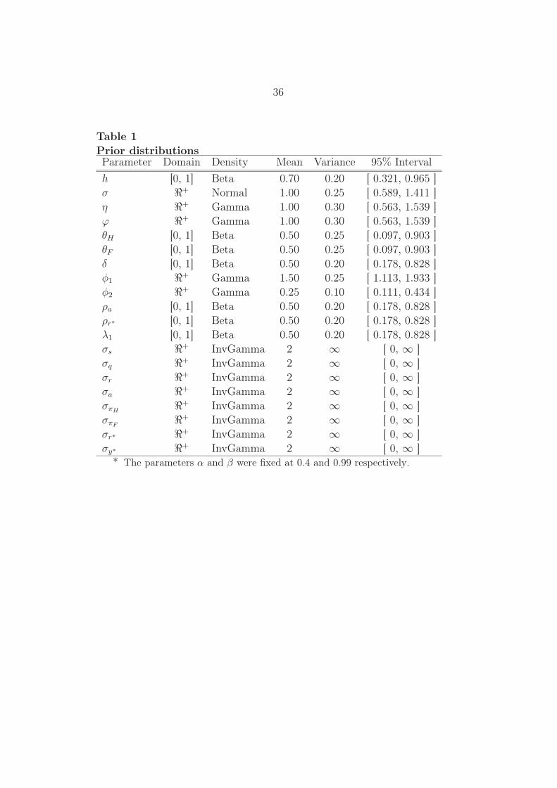
The choice of priors for our estimation are guided by several considerations.At a basic level, the priors reflect our beliefs and the confidence we have aboutthe likely location of the structural parameters. Information on the structuralcharacteristics of the New Zealand economy, such as the degree of openness,being a commodity producer and its institutional settings, were all takeninto account. In the case of New Zealand, micro-level studies were relativelyscarce. Priors from similar studies using New Zealand data for exampleLubik and Schorfheide (2003), and Justiniano and Preston (2004) were alsoconsidered. The Reserve Bank’s main macro model FPS is taken as a goodapproximation of the Bank’s view of the New Zealand economy, and keyparameters contained in FPS and its implied dynamic properties were usedto inform our choice of priors. Finally, the choice of prior distributions reflectrestrictions on the parameters such as non-negativity or interval restrictions.Beta distributions were chosen for parameters that are constrained on theunit-interval. Gamma and normal distributions were selected for parametersin <+, while the inverse gamma distribution was used for the precision of theshocks.
The priors on the model’s parameters are assumed to be independent of eachother, which allows for easier construction of the joint prior density usedin the MCMC algorithm. Furthermore, the parameter space is truncated toavoid indeterminacy or non-uniqueness in the model’s solution. The marginalprior distributions for the model’s parameters are summarized in table (1).
4.3 Estimation and convergence diagnostics
To avoid the problem of stochastic singularity in the case where there aremore observed variables than the number of shocks, three iid N(0,1) mea-surement errors were added to the LRE system. An advantage of addingmeasure errors is that it allows one to change the observed variables for themodel across different specifications. νs
t and νqt can be interpreted as devia-
tions from the definition of the TOT and UIP implied by the model. Lastly,νr
t can be used to measure the monetary surprises by the Reserve Bank asdeviations from the specified reaction function.8 Apart from the interest rate and inflation data which are already in percentage terms.

19
Given the data and the prior specifications in section 4.2, we generate twoparallel 1,500,000 draws9 of the Markov chain using the method describedearlier. The Markov chain is generated conditional on the degree of openness(α) and the time preference (β) parameters, which are fixed at 0.4 and 0.99respectively.
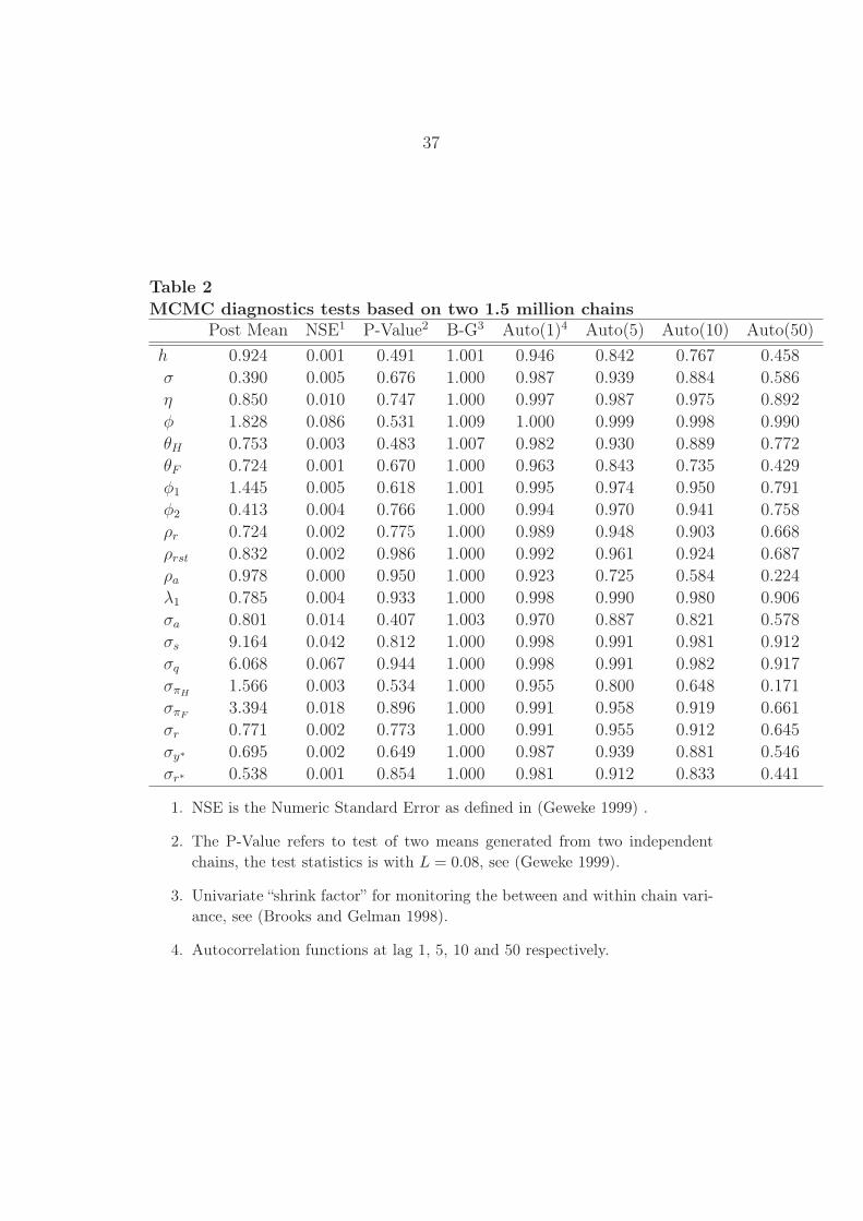
Various convergence diagnostic statistics were computed. The first columnof Table (2) shows the mean of the posterior distribution. The NSE refersto the numeric standard error as the approximation of the true posteriormoment and the p-value is the test between the means generated from twoindependent chains as in Geweke (1999). There is no indication that the twomeans are significantly different from each other. The fourth column showsthe univariate “shrink factor” using the ratio of between and within variancesas in Brooks and Gelman (1998). A shrink factor close to 1 is evidence forconvergence to a stationary distribution. The autocorrelations statistics areshown in column 5 to 8. The multivariate “shrink factor” was computed tobe 1.0117. All MCMC diagnostic tests suggest that the Markov chains hasconverged to its stationary distribution after 1.5 million iterations.
5 Estimation results
5.1 Posterior parameter estimates
Based on the two independent Markov Chains,10 we compute the posteriormean, median and the 95 percent probability intervals for each of the pa-rameters, with results reported in Table 3. The prior and the estimatedposterior marginal densities are plotted in Figure 1. The plots indicate thereis a significant amount of information contained in the data that can be usedto update our prior beliefs about the model’s parameters. The posterior mar-ginal densities are much more concentrated compare than the prior densitieswith the exception of φ (the inverse elasticity of labour supply).
Our results show there is a relatively high degree of external habit persistencewith hm = 0.92 (the superscript m denotes the median of the posterior9 Each chain is generated at different starting values. It takes approximately 120 CPUhours to generate each independent chain using the APAC linux cluster machine.
10 The reported statistics are computed after eliminating the first 40 percent of the MarkovChain (burn-in).

20
distribution) compared with other studies for the US and the euro area, egSmets and Wouters (2004) and Lubik and Schorfheide (2005). The medianof the inverse elasticity of intertemporal substitution, σ, is estimated to be0.39. Smaller values of σ imply that households are less willing to acceptdeviations from a uniform pattern of consumption over time. This low valueseems to be consistent with the relatively high degree of habit persistencediscussed earlier. The posterior median for the elasticity of substitutionbetween home and foreign goods, η, is around 0.85. The relatively low valuefor η is in line with our prior that New Zealand is a commodity-producerand its consumption basket relies heavily on foreign produced goods. Theestimated inverse elasticity of substitution for labour, ϕ, turns out to bemuch greater than 1. This means a 1 percent increase in the real wage willresult in only a small change in labour supply.
On the supply side, the median estimate of the probability of not changingprice in a given quarter, or equivalently the proportion of firms that do notre-optimize their prices in a given quarter, is around 75 percent for domesticfirms and slightly lower for import retailers at 72 percent. These Calvocoefficients imply that the average duration of price contracts is around fourquarters for domestic firms and three quarters for import retailers.11 Thisaggregate degree of nominal price rigidity is much lower than that reportedfor the euro area, but is comparable with estimates for the US.
The simple reaction function used in the model provides a fairly good descrip-tion of monetary policy over the stable inflation period in New Zealand. Theposterior median for the degree of interest rate smoothing is estimated to be0.72 with 1.45 and 0.41 being the weight on inflation and output respectively.
5.2 Impulse response analysis
Figures 2 to 7 plots the impulse functions of the economy in respond to aone unit increase in the various structural and non-structural shocks. Dueto computational difficulties, these impulses were calculated using 10,000random draws from the model’s empirical posterior distribution rather thantaking the full 1.5 million Markov chains. The median impulse responsesare drawn in solid lines while the dotted lines represent the 5th and 95th
percentiles evaluated at each point in time.11 Duration = 1
1−θi.

21
Figure 2 shows that following a temporary positive labour productivity shock,consumption is higher on impact and stays above zero until some 30 quarterslater. Output, on the other hand, stays relatively static on impact and de-crease slightly before staying above trend until 40 quarters later. The strongpersistence in the impulse response can be attributed to the high degree ofpersistence in the estimated productivity shock.12 The initial decrease inoutput suggests that agent’s substitution between working and leisure domi-nates the lower cost of production that arises from the increase in productiv-ity. The impulse analysis suggests that the positive impact on output doesnot come around until five to six quarters later. Inflation falls initially asthe higher labour productivity helps reduce the cost of production before re-turning close to zero 40 quarters later. In this particular case, the monetaryauthority can afford to loosen monetary policy to bring inflation back to zero.The exchange rate initially appreciates before responding to the monetaryloosening via the UIP condition.
Figure 3 shows the effects of a positive import inflation shock. Both domesticand overall inflation are higher on impact, with higher import prices pushingup the cost of production. The higher foreign prices relative to domesticprices increase the degree of competitiveness for the domestic economy. Thiswill see domestic agents substitute out of foreign produced goods into homeproduced goods in response to the price signal – the expenditure switchingeffect from improvements in the domestic economy’s terms of trade. Fromthe impulse responses, this has a positive and significant impact on domes-tic output. The monetary authority responds to the higher overall inflationand output by raising interest rates by 40 basis point before slowly returningto equilibrium over 8 quarters. The higher interest rate appreciates the ex-change rate which acts as another channel to bring both import and domesticinflation back to zero.
Figure 4 shows the effects of a positive domestic inflation shock (which can beinterpreted as a supply shock). Initially, the higher rate of domestic inflationrelative to import inflation decreases the degree of domestic competitivenessby about 1 percent. The monetary authority respond to the higher rate of in-flation by increasing the interest rate by 28 basis points and reaching a peakof 38 basis points in the third quarter before slowly coming back to equi-librium. Domestic output stays relatively static initially before decreasing12 The estimated AR(1) coefficient of 0.98 on the labor productivity tend to suggest a
unit root maybe present in the linearly detrended output data.
22
in response to the monetary tightening. There a significant output-inflationtradeoff in face of the aggregate supply shock. The monetary tightening alsoleads to an appreciation of the exchange rate which act as another channelto bring inflation back to equilibrium.
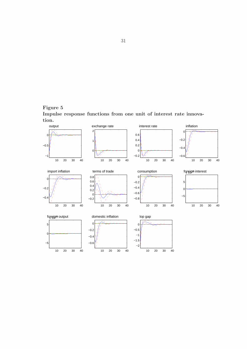
Figure 5 shows a monetary tightening, a 1 percent increase in the interestrate. Immediately after the shock, consumption, output and overall inflationfall by 0.6 percent, 0.8 percent and 0.4 percent respectively. The consump-tion response is hump-shaped because, under habit formation, agents smoothboth the level and the change of consumption. The peak consumption re-sponse takes place after two quarters. Output, on the other hand, does notexperience the same hump-shape response. The inclusion of stock adjust-ment, in particular introducing capital into the model, may help improvethe dynamic response of output, enabling it to reproduce the hump-shapedresponse usually found in VAR models.
The 1 percent increase in the interest rate has a peak influence on overallinflation of 0.5 percent, which is reached after three quarters. Due to theinitial negative impact on output and inflation, the 1 percent interest rateinnovation only results in a 0.6 percent increase in the nominal interest rate.This decreases quickly below zero after 2 quarters before adjusting slowly torestore both inflation and output back to its equilibrium. The exchange ratereacts positively to the monetary tightening before returning to equilibrium.The model predicts that a 1 percent interest rate shock will result in closeto a 2 percent appreciation of the exchange rate.
Figure 6 shows a 1 percent deviation of the exchange rate from the UIPcondition. Since no extrinsic persistence is assumed for the process of thisshock, the shock has a relatively short-lived effect on the real exchange rate.Consequently, output will be 0.2 percent lower while there will be little effecton consumption. On the other hand, the higher exchange rate decreases bothimport and domestic inflation with overall inflation falling by 0.1 percent.The UIP shock also results in a small monetary expansion: interest ratesdecline by 10 basis points. The temporary exchange rate appreciation haslittle influence on the domestic economy’s terms of trade.
Figure 7 shows a 1 percent increase in st, which corresponds to an improve-ment in international competitiveness for the domestic economy. Followingthe shock, there is an increase in aggregate demand that causes output toincrease while leaving inflation pretty much unchanged. There is no changein overall inflation, due to the opposing effects from import and domestic

23
inflation. This shock has a very minor effect on domestic consumption. Onecan think of the differentials in the output and consumption paths as beingattributed to the increase in exports. The interest rate response is hump-shaped; the peak response (8 basis points) takes place after three quarters.There is a small exchange rate appreciation in response to the monetarytightening which helps offset the higher TOT to some degree. It is not sur-prising that the 1 percent shock has a very minor quantitative impact on theNew Zealand economy given that the estimated standard deviation on termsof trade shock is around 9 percent.
6 Concluding remarks
In this paper, we used Bayesian methods to combine prior information withthe historical data, to develop a small open economy model of the NewZealand economy. The Bayesian approach provided us with a tool to under-stand and learn about the sources of uncertainty imbedded in quantitativemacroeconomic modelling. The model and the set of estimated parameterscan be used to guide future monetary policy questions in New Zealand.
The estimated parameters largely reflected New Zealand’s structural char-acteristics of being a small, relatively open commodity producer. Here wesummarize our main empirical findings. First, there is a high degree of habitformation together with a relatively low degree of intertemporal consumptionsubstitutability. Agents are quite reluctant to deviate from a uniform con-sumption pattern over time. In response to shocks, consumption deviationsfrom equilibrium appears to be relatively small when compared with outputvariation. When adjustments are necessary, there is a high degree of smooth-ing to both the level and the change of consumption. Second, the low degreeof substitutability between home and foreign produced goods reflects NewZealand’s commodity-producer characteristic; New Zealand’s consumptionbasket relies heavily on foreign produced goods that are not close substitutesfor the commodities New Zealand specialises in producing. Third, the lowelasticity for labour supply decisions is partly attributed to the relativelyimmobile work force. However, explicit modelling of the labour market maybe required to gain further insights. Fourth, the average duration of pricecontracts was estimated to be around five quarters for domestic firms andfour quarters for import retailers. Lastly, the impulse response functionspresented in this paper provide a qualitative and quantitative way of under-

24
standing the dynamic behaviour of the economy in response to the variousshocks. These impulse response also enable us to describe the transmissionof monetary policy to the rest of the economy.
In this paper, we restricted ourselves to a relatively simple specification ofthe model with only two sources of nominal rigidities, a linear productionfunction in labour, and a simple role for the central bank. In future research,it would be interesting to expand the model to incorporate other factors ofinterest to policymakers, including: (i) capital accumulation and investmentrigidities; (ii) an explicit government sector with a role for fiscal policy and in-teractions with monetary policy; (iii) labour market rigidities; (iv) in a multisector/good setting; (v) an endogenous foreign sector; and (vi) incompletefinancial markets, to faciliate analysis of current account dynamics. Lastly, itwould also be interesting to investigate the forecasting ability of this DSGEstructure.
References
Bouakez, H, E Cardia, and F J Ruge-Murcia (2005), “Habit formation andthe persistence of monetary shocks,” Journal of Monetary Economics,52, 1073–88.
Brooks, S and A Gelman (1998), “Alternative methods for monitoring conver-gence of iterative simulations,” Journal of Computational and GraphicalStatistics, 7, 434–455.
Buckle, R A, K Kim, and N McLellan (2003), “The impact of monetary policyon New Zealand business cycles and inflation variability,” New ZealandTreasury, Working Paper, 03/09.
Burstein, A T, J C Neves, and S Rebelo (2003), “Distribution costs andreal exchange rate dynamics during exchange-rate-based-stabilizations,”Jornal of Monetary Economics, 50(6), 1189–1214.
Christiano, L J, M Eichenbaum, and C Evans (2005), “Nominal rigiditiesand the dynamic effects of a shock to monetary policy,” The Journal ofPolitical Economy, 113, 1–45.
Clarida, R, J Gali, and M Gertler (2001), “Optimal monetary policy in open
25
versus closed economies: An integrated approach,” American EconomicReview, 91(2), 248–252.
Gali, J and T Monacelli (2005), “Monetary policy and exchange rate volatilityin a small open economy,” Review of Economic Studies, 72(3), 707–34.
Gardiner, P, R Gray, D Hargreaves, and K L Szeto (2003), “A comparison ofthe NZTM and FPS models of the New Zealand economy,” New ZealandTreasury, Working Paper, 03/25.
Geweke, J (1999), “Using simulation methods for Bayesian econometric mod-els,” Society for Computational Economics, Computing in Economicsand Finance 1999, 832.
Justiniano, A and B Preston (2004), “Small open economy DSGE mod-els: Specification, estimation and model fit,” Department of Economics,Columbia University, Working Paper.
Lees, K (2003), “The stabilisation problem: The case of New Zealand,” Re-serve Bank of New Zealand, Discussion Paper, DP2003/08.
Lubik, T and F Schorfheide (2003), “Do central banks respond to exchangerate movements? A structural investigation,” Department of Economics,The Johns Hopkins University, Economics Working Paper Archive, 505.
Lubik, T and F Schorfheide (2005), “A Bayesian look at new open econ-omy macroeconomics,” in NBER Macroeconomics Annual 2005, vol 20,NBER, MIT Press.
Lucas, R E, Jr (1976), “Econometric policy evaluation: A critique,” CarnegieRochester Conference Series on Public Policy, 1, 19–46.
Monacelli, T (2005), “Monetary policy in a low pass-through environment,”Journal of Money Credit and Banking, 37(6), 1047–1066.
Smets, F and R Wouters (2003), “An estimated dynamic stochastic generalequilibrium model of the euro area,” Journal of the European EconomicAssociation, 1(5), 1123–1175.
Smets, F and R Wouters (2004), “An estimated stochastic dynamic generalequilibrium model of the euro area,” Journal of the European EconomicAssociation, 1, 1123–75.
Uhlig, H (1995), “A toolkit for analyzing nonlinear dynamic stochastic models

26
easily,” Federal Reserve Bank of Minneapolis - Instititute for EmpiricalMacroeconomics, Discussion Paper, 101.
Woodford, M (2003), Interest and Prices: Foundations of a Theory of Mon-etary Policy, Princeton University Press, Princeton.
Yun, T (1996), “Nominal rigidities, money supply endogeneity, and businesscycles,” Journal of Monetary Economics, 37, 345–370.

27
Figure 1Posterior and prior marginal density plot
00.5
10 5 10 15
h
02
40 1 2 3
σ
02
40 1 2
η
02
40
0.5 1
φ
00.5
10 5 10 15
θH
00.5
10 10 20
θF
01
23
0 1 2 3
φ1
00.5
10 2 4
φ2
00.5
10 5 10
ρr
00.5
10 5 10
ρrst
00.5
10 10 20 30
ρa
00.5
10 2 4 6 8
λ1

28
Figure 2Impulse response functions from one unit of labour productivityinnovation.
10 20 30 40
−1
−0.5
0
0.5
1
1.5
output
10 20 30 40
0
2
4
6
exchange rate
10 20 30 40
−2
−1
0
interest rate
10 20 30 40−3
−2
−1
0
1
inflation
10 20 30 40
−3
−2.5
−2
−1.5
−1
−0.5
import inflation
10 20 30 40
−6
−4
−2
0
2
terms of trade
10 20 30 40
2
4
6
8consumption
10 20 30 40−1
−0.5
0
0.5
1x 10
−14foreign interest
10 20 30 40
−5
0
5
x 10−15foreign output
10 20 30 40
−2
0
2
domestic inflation
10 20 30 40
−4
−2
0
lop gap

29
Figure 3Impulse response functions from one unit of import inflation inno-vation.
10 20 30 40
0
0.2
0.4
output
10 20 30 40
0
0.5
1
1.5
exchange rate
10 20 30 40
0
0.2
0.4
interest rate
10 20 30 40
0
0.2
0.4
0.6
0.8
inflation
10 20 30 40
0
0.5
1
import inflation
10 20 30 40
0
0.5
1
terms of trade
10 20 30 40
0
0.5
1
consumption
10 20 30 40
−1
−0.5
0
0.5
1
x 10−15foreign interest
10 20 30 40
−5
0
5
x 10−16foreign output
10 20 30 400
0.2
0.4
0.6
domestic inflation
10 20 30 40
−2
−1.5
−1
−0.5
0
lop gap

30
Figure 4Impulse response functions from one unit of domestic inflation in-novation.
10 20 30 40−0.6
−0.4
−0.2
0
output
10 20 30 40
0
0.2
0.4
0.6
exchange rate
10 20 30 400
0.1
0.2
0.3
0.4
interest rate
10 20 30 40
0
0.2
0.4
0.6
inflation
10 20 30 40
−0.1
0
0.1
0.2
0.3
0.4
import inflation
10 20 30 40−2
−1.5
−1
−0.5
0
0.5
terms of trade
10 20 30 40
0
0.2
0.4
0.6
0.8
consumption
10 20 30 40−2
−1
0
1
2x 10
−15foreign interest
10 20 30 40
−1
−0.5
0
0.5
1
x 10−15foreign output
10 20 30 40
0
0.5
1
domestic inflation
10 20 30 40
−0.5
0
0.5
lop gap
31
Figure 5Impulse response functions from one unit of interest rate innova-tion.
10 20 30 40
−1
−0.5
0
output
10 20 30 40
0
1
2
exchange rate
10 20 30 40
−0.2
0
0.2
0.4
0.6
interest rate
10 20 30 40
−0.6
−0.4
−0.2
0
inflation
10 20 30 40
−0.4
−0.2
0
import inflation
10 20 30 40
−0.2
0
0.2
0.4
0.6
0.8
terms of trade
10 20 30 40
−0.8
−0.6
−0.4
−0.2
0
consumption
10 20 30 40
−5
0
5
x 10−16foreign interest
10 20 30 40
−5
0
5
x 10−16foreign output
10 20 30 40
−0.6
−0.4
−0.2
0
domestic inflation
10 20 30 40
−2
−1.5
−1
−0.5
0
lop gap

32
Figure 6Impulse response functions from one unit of exchange rate innova-tion.
10 20 30 40
−0.3
−0.2
−0.1
0
output
10 20 30 40−0.2
0
0.2
0.4
0.6
0.8
exchange rate
10 20 30 40
−0.1
−0.05
0
interest rate
10 20 30 40
−0.08
−0.06
−0.04
−0.02
0
inflation
10 20 30 40
−0.1
−0.05
0
import inflation
10 20 30 40
−0.05
0
0.05
terms of trade
10 20 30 40
−0.1
−0.05
0
0.05
0.1
consumption
10 20 30 40
−1
−0.5
0
0.5
1
x 10−16foreign interest
10 20 30 40
−5
0
5
x 10−17foreign output
10 20 30 40
−0.1
−0.05
0
domestic inflation
10 20 30 40−0.8
−0.6
−0.4
−0.2
0
0.2
lop gap

33
Figure 7Impulse response functions from one unit of competitiveness inno-vation.
10 20 30 40−0.1
0
0.1
0.2
output
10 20 30 40−0.1
−0.05
0
0.05
0.1
0.15
exchange rate
10 20 30 40
−0.02
0
0.02
0.04
0.06
0.08
interest rate
10 20 30 40−0.01
0
0.01
0.02
0.03
inflation
10 20 30 40−0.2
−0.15
−0.1
−0.05
0
0.05
import inflation
10 20 30 40−0.4
−0.2
0
0.2
0.4
0.6
0.8
terms of trade
10 20 30 40−0.06
−0.04
−0.02
0
0.02
0.04consumption
10 20 30 40
−2
0
2
x 10−16foreign interest
10 20 30 40
−2
0
2
x 10−16foreign output
10 20 30 40
0
0.05
0.1
domestic inflation
10 20 30 40−0.6
−0.4
−0.2
0
0.2
lop gap

34
Appendix
A The linearized model
1. Law of one price gap
ψt = −[qt + (1− α)st]
2. Terms of trade with measurement error:
∆st = πF,t − πH,t + νst
3. Uncovered interest parity condition with a risk premium shock:
∆Etqt+1 = −(rt − Etπt+1)− (r∗t − Etπ∗t+1)+ νq
t
4. Domestic inflation:
πH,t = β(1− θH)EtπH,t+1 + θHπH,t−1 + λHmct + νπHt
5. Import inflation:
πF,t = β(1− θF )EtπH,t+1 + θF πF,t−1 + λF ψt + νπFt
6. Overall inflation:πt = (1− α)πH,t + απF,t
7. Firm’s marginal cost:
mct =σ
1− h(ct − hct−1) + ϕyt + αst − (1 + ϕ)at
8. Consumption Euler equation:
ct − hct−1 = Et(ct+1 − hct)− 1− h
σ(rt − Etπt+1)
9. International risk sharing condition:
ct − hct−1 = y∗t − hy∗t−1 −1− h
σqt
35
10. Goods market clearing condition:
yt = (2− α)αηst + (1− α)ct + αηψt + αy∗t
11. Reaction function:
rt = ρrrt−1 + (1− ρr)(φ1πt + φ2∆yt) + νrt
12. Exogenous processes:at = ρaat−1 + νa
t
y∗t = λ1y∗ + νy∗
t
(r∗t − Etπ∗t+1) = ρr∗(r
∗t−1 − π∗t ) + νr∗
t
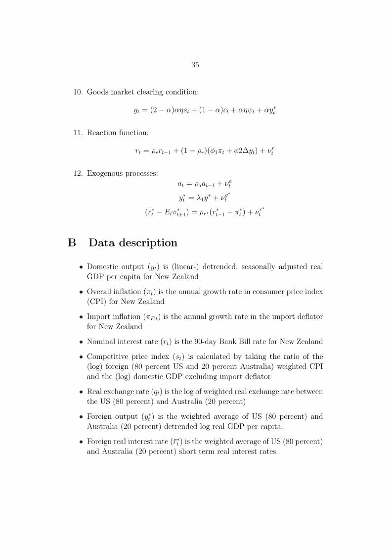
B Data description
• Domestic output (yt) is (linear-) detrended, seasonally adjusted realGDP per capita for New Zealand
• Overall inflation (πt) is the annual growth rate in consumer price index(CPI) for New Zealand
• Import inflation (πF,t) is the annual growth rate in the import deflatorfor New Zealand
• Nominal interest rate (rt) is the 90-day Bank Bill rate for New Zealand
• Competitive price index (st) is calculated by taking the ratio of the(log) foreign (80 percent US and 20 percent Australia) weighted CPIand the (log) domestic GDP excluding import deflator
• Real exchange rate (qt) is the log of weighted real exchange rate betweenthe US (80 percent) and Australia (20 percent)
• Foreign output (y∗t ) is the weighted average of US (80 percent) andAustralia (20 percent) detrended log real GDP per capita.
• Foreign real interest rate (r∗t ) is the weighted average of US (80 percent)and Australia (20 percent) short term real interest rates.
36
Table 1Prior distributionsParameter Domain Density Mean Variance 95% Intervalh [0, 1] Beta 0.70 0.20 [ 0.321, 0.965 ]σ <+ Normal 1.00 0.25 [ 0.589, 1.411 ]η <+ Gamma 1.00 0.30 [ 0.563, 1.539 ]ϕ <+ Gamma 1.00 0.30 [ 0.563, 1.539 ]θH [0, 1] Beta 0.50 0.25 [ 0.097, 0.903 ]θF [0, 1] Beta 0.50 0.25 [ 0.097, 0.903 ]δ [0, 1] Beta 0.50 0.20 [ 0.178, 0.828 ]φ1 <+ Gamma 1.50 0.25 [ 1.113, 1.933 ]φ2 <+ Gamma 0.25 0.10 [ 0.111, 0.434 ]ρa [0, 1] Beta 0.50 0.20 [ 0.178, 0.828 ]ρr∗ [0, 1] Beta 0.50 0.20 [ 0.178, 0.828 ]λ1 [0, 1] Beta 0.50 0.20 [ 0.178, 0.828 ]σs <+ InvGamma 2 ∞ [ 0, ∞ ]σq <+ InvGamma 2 ∞ [ 0, ∞ ]σr <+ InvGamma 2 ∞ [ 0, ∞ ]σa <+ InvGamma 2 ∞ [ 0, ∞ ]σπH
<+ InvGamma 2 ∞ [ 0, ∞ ]σπF
<+ InvGamma 2 ∞ [ 0, ∞ ]σr∗ <+ InvGamma 2 ∞ [ 0, ∞ ]σy∗ <+ InvGamma 2 ∞ [ 0, ∞ ]* The parameters α and β were fixed at 0.4 and 0.99 respectively.
37
Table 2MCMC diagnostics tests based on two 1.5 million chains
Post Mean NSE1 P-Value2 B-G3 Auto(1)4 Auto(5) Auto(10) Auto(50)h 0.924 0.001 0.491 1.001 0.946 0.842 0.767 0.458σ 0.390 0.005 0.676 1.000 0.987 0.939 0.884 0.586η 0.850 0.010 0.747 1.000 0.997 0.987 0.975 0.892φ 1.828 0.086 0.531 1.009 1.000 0.999 0.998 0.990θH 0.753 0.003 0.483 1.007 0.982 0.930 0.889 0.772θF 0.724 0.001 0.670 1.000 0.963 0.843 0.735 0.429φ1 1.445 0.005 0.618 1.001 0.995 0.974 0.950 0.791φ2 0.413 0.004 0.766 1.000 0.994 0.970 0.941 0.758ρr 0.724 0.002 0.775 1.000 0.989 0.948 0.903 0.668ρrst 0.832 0.002 0.986 1.000 0.992 0.961 0.924 0.687ρa 0.978 0.000 0.950 1.000 0.923 0.725 0.584 0.224λ1 0.785 0.004 0.933 1.000 0.998 0.990 0.980 0.906σa 0.801 0.014 0.407 1.003 0.970 0.887 0.821 0.578σs 9.164 0.042 0.812 1.000 0.998 0.991 0.981 0.912σq 6.068 0.067 0.944 1.000 0.998 0.991 0.982 0.917σπH
1.566 0.003 0.534 1.000 0.955 0.800 0.648 0.171σπF
3.394 0.018 0.896 1.000 0.991 0.958 0.919 0.661σr 0.771 0.002 0.773 1.000 0.991 0.955 0.912 0.645σy∗ 0.695 0.002 0.649 1.000 0.987 0.939 0.881 0.546σr∗ 0.538 0.001 0.854 1.000 0.981 0.912 0.833 0.441
1. NSE is the Numeric Standard Error as defined in (Geweke 1999) .
2. The P-Value refers to test of two means generated from two independentchains, the test statistics is with L = 0.08, see (Geweke 1999).
3. Univariate “shrink factor” for monitoring the between and within chain vari-ance, see (Brooks and Gelman 1998).
4. Autocorrelation functions at lag 1, 5, 10 and 50 respectively.

38
Table 3Posterior estimates using 1.5 million Markov chain drawsParameter Prior mean Post. median Post. 95% intervalh 0.70 0.92 [ 0.88, 0.96 ]σ 1.00 0.39 [ 0.19, 0.68 ]η 1.00 0.85 [ 0.58, 1.16 ]ϕ 1.00 1.83 [ 0.83, 3.14 ]θH 0.50 0.75 [ 0.71, 0.80 ]θF 0.50 0.72 [ 0.69, 0.76 ]φ1 1.50 1.44 [ 1.27, 1.67 ]φ2 0.25 0.41 [ 0.28, 0.58 ]δ 0.50 0.72 [ 0.65, 0.79 ]ρr∗ 0.50 0.83 [ 0.76, 0.89 ]ρa 0.50 0.98 [ 0.95, 0.99 ]λ1 0.50 0.78 [ 0.67, 0.87 ]σa [0,∞] 0.80 [ 0.49, 1.27 ]σs [0,∞] 9.16 [ 7.63, 11.08 ]σq [0,∞] 6.07 [ 4.68 , 8.10 ]σπH
[0,∞] 1.57 [ 1.27, 1.94 ]σπF
[0,∞] 3.39 [ 2.70, 4.30 ]σr [0,∞] 0.77 [ 0.64, 0.94 ]σy∗ [0,∞] 0.69 [ 0.58, 0.84 ]σr∗ [0,∞] 0.54 [ 0.44, 0.66 ]* The parameters α and β were fixed at 0.4 and 0.99 respectively.