drill cuttings and muds dispersion modelling - epa...2018/04/03 · model, mudmap, to predict the...

Annex E

Drill Cuttings and Muds Dispersion Modelling

rpsgroup.com.au

REPORT

Tamarind - Tui Field Drill Cuttings and Muds Dispersion Modelling

Prepared by: RPS AUSTRALIA WEST PTY LTD

Suite E1, Level 4

140 Bundall Road

Bundall, QLD 4217

Australia

Prepared for: ERM NEW ZEALAND

117 Powderham St

New Plymouth 4310

New Zealand

T: +61 7 5574 1112 T: +64 (0)9 3034 664

E: [email protected] E: [email protected]

W: erm.com.au

Author: Nathan Benfer

Reviewed: Sasha Zigic

Approved: Nathan Benfer

No.: MAQ0648J

Version: 2

Date: 21/03/2018

MAQ0648J | Tamarind - Tui Field | Drill Cuttings and Muds Dispersion Modelling | 21/03/2018

Page II

REPORT

Document Status

Version Purpose of Document Approved by Reviewed by Review Date

0 Draft Issued to Client Nathan Benfer Sasha Zigic 31/01/2018

1 Issued to Client Nathan Benfer Sasha Zigic 12/02/2018

2 Issued to Client Nathan Benfer Sasha Zigic 21/03/2018

Approval for issue

Name Signature Date

Nathan Benfer

21/03/2018

This report was prepared by [RPS Australia West Pty Ltd (‘RPS’)] within the terms of its engagement and in direct response to a scope of services. This report is strictly limited to the purpose and the facts and matters stated in it and does not apply directly or indirectly and must not be used for any other application, purpose, use or matter. In preparing the report, RPS may have relied upon information provided to it at the time by other parties. RPS accepts no responsibility as to the accuracy or completeness of information provided by those parties at the time of preparing the report. The report does not take into account any changes in information that may have occurred since the publication of the report. If the information relied upon is subsequently determined to be false, inaccurate or incomplete then it is possible that the observations and conclusions expressed in the report may have changed. RPS does not warrant the contents of this report and shall not assume any responsibility or liability for loss whatsoever to any third party caused by, related to or arising out of any use or reliance on the report howsoever. No part of this report, its attachments or appendices may be reproduced by any process without the written consent of RPS. All enquiries should be directed to RPS.


Page III

REPORT

Contents EXECUTIVE SUMMARY .................................................................................................................................... 6

1 INTRODUCTION ................................................................................................................................. 8 1.1 Project Background .......................................................................................................................... 8

2 SCOPE OF WORK ........................................................................................................................... 10

3 REGIONAL CURRENTS .................................................................................................................. 10 3.1Tidal Currents ............................................................................................................................................ 12 3.1.1Grid Setup ................................................................................................................................................. 12 3.1.2 Tidal Conditions ....................................................................................................................................... 14 3.1.3 Surface Elevation Validation ............................................................................................................. 14 3.2 Ocean Currents ............................................................................................................................... 19 3.3 Currents at the Release Site .......................................................................................................... 20

4 WATER TEMPERATURE AND SALINITY ...................................................................................... 22

5 SEDIMENT DISPERSION MODELLING .......................................................................................... 24 5.1 Model Description - MUDMAP ........................................................................................................ 24 5.2 Discharge Program ......................................................................................................................... 25 5.3 Discharge Input Data ...................................................................................................................... 26 5.4 Grid Configuration .......................................................................................................................... 29 5.5 Mixing Parameters .......................................................................................................................... 29 5.6 Minimum Reporting Thresholds .................................................................................................... 29

6 RESULTS .......................................................................................................................................... 30

7 REFERENCES .................................................................................................................................. 36


Page IV

REPORT

Tables Table 1 Coordinates of the release sites used in the study. ....................................................................... 8 Table 2 Statistical comparison between the observed and HYDROMAP predicted surface elevations

data from the 1st to 31st January 2014. ........................................................................................ 15 Table 3 Predicted average and maximum surface current speeds at the study site. The data was

derived by combining the HYCOM ocean data and HYDROMAP tidal data for 2008-2012 (inclusive). .................................................................................................................................... 20

Table 4 Monthly average sea-surface temperature and salinity at the study area. .................................. 22 Table 5 Summary of the estimated volume of discharged drill cuttings and unrecoverable mud solids for

each well. ..................................................................................................................................... 26 Table 6 Input data used for the drill cuttings and unrecoverable mud solids dispersion modelling. ......... 27 Table 7 Discharged grain size distribution and settling velocities assumed for the production wells

consisting of cuttings and water-based mud. ............................................................................... 28 Table 8 Predicted bottom deposition, area of coverage and maximum distance to the minimum

threshold for each well. ................................................................................................................ 31 Table 9 Total area covered for each bottom deposition range for Amokura-2H. ...................................... 31 Table 10 Total area covered for each bottom deposition range for Tui-2H and 3H combined. .................. 31 Table 11 Total area covered for each bottom deposition range for Pateke-3H. ......................................... 31 Table 12 Predicted total suspended solids concentration for each well ..................................................... 32 Table 13 Total area covered for each total suspended solids concentration range for Amokura-2H. ........ 32 Table 14 Total area covered for each total suspended solids concentration range forTui-2H and 3H

combined. ..................................................................................................................................... 32 Table 15 Total area covered for each total suspended solids concentration range for Pateke-3H. ........... 32


Page V

REPORT

Figures Figure 1 Location of the release sites used in the modelling study. ............................................................ 9 Figure 2 Schematic showing the oceanic current circulation surrounding New Zealand (Image source:

Brodie, 1960). ............................................................................................................................... 11 Figure 3 Map showing the regions of sub-gridding for the study area ....................................................... 13 Figure 4 Bathymetry used in the hydrodynamic grid for the study region. ................................................. 13 Figure 5 Location of the nine tide stations around New Zealand used to validate the tidal model. ........... 15 Figure 6 Comparison between predicted (red line) and observed (blue line) surface elevation variation at

Auckland (top), Bluff (middle) and Lyttelton (bottom), between the 1st and the 31st of January 2014. ............................................................................................................................................ 16

Figure 7 Comparison between predicted (red line) and observed (blue line) surface elevation variation at Napier (top), Nelson (middle) and Picton (bottom), between the 1st and the 31st of January 2014. ..................................................................................................................................................... 17

Figure 8 Comparison between predicted (red line) and observed (blue line) surface elevation variation at Port Taranaki (top), Wellington (middle) and Westport (bottom), between the 1st and 31st of January 2014................................................................................................................................ 18

Figure 9 Snapshot example of the predicted HYCOM ocean surface currents in the region. Colour of individual arrows indicate current speed (m/s). ............................................................................ 19

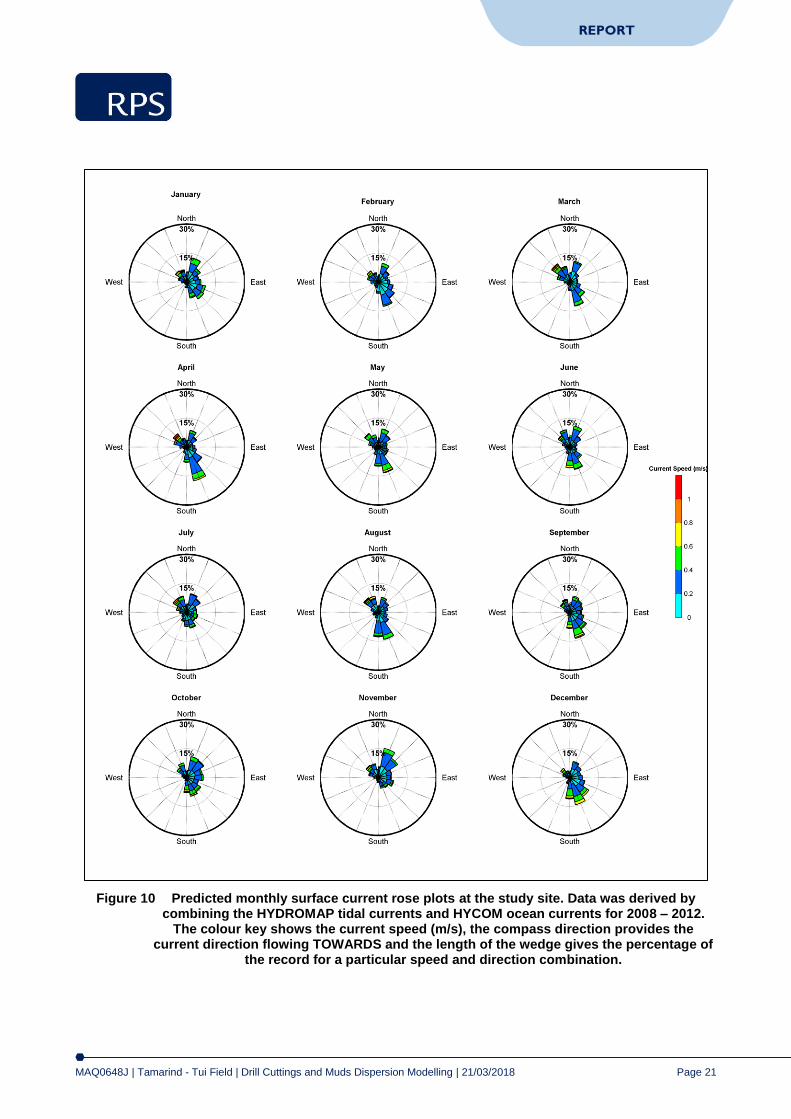
Figure 10 Predicted monthly surface current rose plots at the study site. Data was derived by combining the HYDROMAP tidal currents and HYCOM ocean currents for 2008 – 2012. The colour key shows the current speed (m/s), the compass direction provides the current direction flowing TOWARDS and the length of the wedge gives the percentage of the record for a particular speed and direction combination. ................................................................................................ 21

Figure 11 Monthly average sea temperature and salinity profiles at the study site. .................................... 23 Figure 12 Conceptual diagram showing the general behaviour of cuttings and muds following discharge to

the ocean (Neff, 2005) and the idealised representation of the three discharge phases. ........... 25 Figure 13 Predicted bottom deposition and coverage from drill cuttings and unrecoverable mud solids on

the seafloor for Amokura-2H. ....................................................................................................... 33 Figure 14 Predicted bottom deposition and coverage from drill cuttings and unrecoverable mud solids on

the seafloor for Tui-2H and 3H combined. ................................................................................... 33 Figure 15 Predicted bottom deposition and coverage from drill cuttings and unrecoverable mud solids on

the seafloor for Pateke-3H. .......................................................................................................... 34 Figure 16 Predicted peak total suspended solids from drill cuttings and unrecoverable mud solids in the

water column for Amokura-2H. .................................................................................................... 34 Figure 17 Predicted peak total suspended solids from drill cuttings and unrecoverable mud solids in the

water column for Tui-2H and 3H combined. ................................................................................ 35 Figure 18 Predicted peak total suspended solids from drill cuttings and unrecoverable mud solids in the

water column for Pateke-3H. ........................................................................................................ 35


Page 6

REPORT

Executive Summary

Project Background

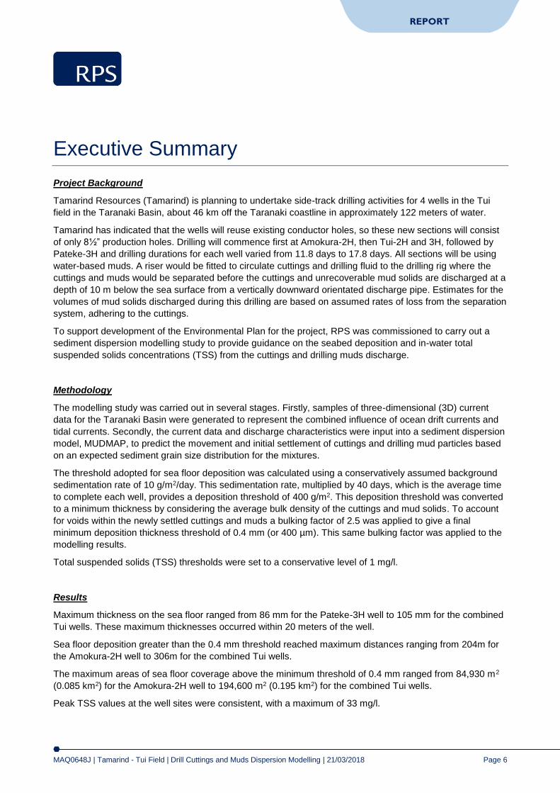
Tamarind Resources (Tamarind) is planning to undertake side-track drilling activities for 4 wells in the Tui field in the Taranaki Basin, about 46 km off the Taranaki coastline in approximately 122 meters of water.

Tamarind has indicated that the wells will reuse existing conductor holes, so these new sections will consist of only 8½” production holes. Drilling will commence first at Amokura-2H, then Tui-2H and 3H, followed by Pateke-3H and drilling durations for each well varied from 11.8 days to 17.8 days. All sections will be using water-based muds. A riser would be fitted to circulate cuttings and drilling fluid to the drilling rig where the cuttings and muds would be separated before the cuttings and unrecoverable mud solids are discharged at a depth of 10 m below the sea surface from a vertically downward orientated discharge pipe. Estimates for the volumes of mud solids discharged during this drilling are based on assumed rates of loss from the separation system, adhering to the cuttings.

To support development of the Environmental Plan for the project, RPS was commissioned to carry out a sediment dispersion modelling study to provide guidance on the seabed deposition and in-water total suspended solids concentrations (TSS) from the cuttings and drilling muds discharge.

Methodology

The modelling study was carried out in several stages. Firstly, samples of three-dimensional (3D) current data for the Taranaki Basin were generated to represent the combined influence of ocean drift currents and tidal currents. Secondly, the current data and discharge characteristics were input into a sediment dispersion model, MUDMAP, to predict the movement and initial settlement of cuttings and drilling mud particles based on an expected sediment grain size distribution for the mixtures.

The threshold adopted for sea floor deposition was calculated using a conservatively assumed background sedimentation rate of 10 g/m2/day. This sedimentation rate, multiplied by 40 days, which is the average time to complete each well, provides a deposition threshold of 400 g/m2. This deposition threshold was converted to a minimum thickness by considering the average bulk density of the cuttings and mud solids. To account for voids within the newly settled cuttings and muds a bulking factor of 2.5 was applied to give a final minimum deposition thickness threshold of 0.4 mm (or 400 µm). This same bulking factor was applied to the modelling results.

Total suspended solids (TSS) thresholds were set to a conservative level of 1 mg/l.

Results

Maximum thickness on the sea floor ranged from 86 mm for the Pateke-3H well to 105 mm for the combined Tui wells. These maximum thicknesses occurred within 20 meters of the well.

Sea floor deposition greater than the 0.4 mm threshold reached maximum distances ranging from 204m for the Amokura-2H well to 306m for the combined Tui wells.

The maximum areas of sea floor coverage above the minimum threshold of 0.4 mm ranged from 84,930 m2 (0.085 km2) for the Amokura-2H well to 194,600 m2 (0.195 km2) for the combined Tui wells.

Peak TSS values at the well sites were consistent, with a maximum of 33 mg/l.


Page 7

REPORT

Maximum peak TSS values greater than the 1 mg/l threshold reached maximum distances ranging from 500 m for the Amokura-2H well to 571 m for the Pateke-3H well.

The total areas of influence by TSS values greater than the threshold of 1 mg/l ranged from 282,390 m2 (0.282 km2) for the Amokura-2H well to 604,000 m2 (0.604 km2) for the combined Tui wells.

TSS concentrations of 10 mg/l were only observed in the top 20 m of the water column, while TSS concentrations down to 2 mg/l were only observed down to 30 or 40 m.

TSS concentrations greater than 1 mg/l extended almost all the way to the seabed directly under the discharge site, due to material falling through this column of water, however further afield TSS concentrations greater than 1 mg/l were only observed in the top 30 to 40 m of the water column.


Page 8

REPORT

1 Introduction

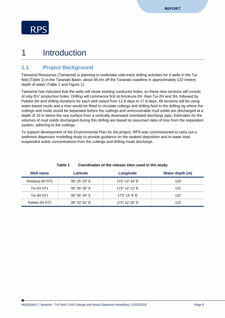
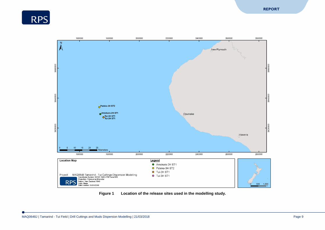
1.1 Project Background Tamarind Resources (Tamarind) is planning to undertake side-track drilling activities for 4 wells in the Tui field (Table 1) in the Taranaki Basin, about 46 km off the Taranaki coastline in approximately 122 meters depth of water (Table 1 and Figure 1).

Tamarind has indicated that the wells will reuse existing conductor holes, so these new sections will consist of only 8½” production holes. Drilling will commence first at Amokura-2H, then Tui-2H and 3H, followed by Pateke-3H and drilling durations for each well varied from 11.8 days to 17.8 days. All sections will be using water-based muds and a riser would be fitted to circulate cuttings and drilling fluid to the drilling rig where the cuttings and muds would be separated before the cuttings and unrecoverable mud solids are discharged at a depth of 10 m below the sea surface from a vertically downward orientated discharge pipe. Estimates for the volumes of mud solids discharged during this drilling are based on assumed rates of loss from the separation system, adhering to the cuttings.

To support development of the Environmental Plan for the project, RPS was commissioned to carry out a sediment dispersion modelling study to provide guidance on the seabed deposition and in-water total suspended solids concentrations from the cuttings and drilling muds discharge.

Table 1 Coordinates of the release sites used in the study.

Well name Latitude Longitude Water depth (m)

Amokura-2H ST1 39° 25’ 23” S 173° 12’ 44” E 123

Tui-2H ST1 39° 26’ 35” S 173° 14’ 11” E 122

Tui-3H ST1 39° 26’ 34” S 173° 14’ 9” E 122

Pateke-3H ST2 39° 22’ 52” S 173° 12’ 25” E 123


Page 9

REPORT

Figure 1 Location of the release sites used in the modelling study.


Page 10

REPORT

2 Scope of Work

The scope of work included the following components:

Generate three-dimensional (3D) currents for the study area that includes the combined influence of ocean and tidal currents for 2012;

Summarise the drilling plans and discharge characteristics as input into the sediment dispersion model, MUDMAP;

Simulate all stages of the drilling programme; and

Analyse and process the MUDMAP results to map the distribution and thicknesses of discharged cuttings and muds on the sea floor and concentrations of total suspended solids (TSS) in the upper water column.

3 Regional Currents

An extensive review of the ocean circulation surrounding New Zealand, which describes the ocean currents in the region, is provided by Heath (1985). The study describes two main surface water masses which surround New Zealand, which include the Subtropical and Subantarctic Surface waters. The Subtropical waters predominately originate from an extension of the East Australian Current (EAC), which is a western boundary current that flows from the South Equatorial Current (SEC), and down the eastern coast of Australia. Typically, the EAC carries warm waters to the south, before splitting off into the Tasman Sea approximately in line with Sydney (Coleman, 1984) and carrying the warmer waters eastwards towards New Zealand (Heath, 1985). The Subantarctic Water tends to flow northwards along the eastern side of the South Island, originating from the Circumpolar Current south of New Zealand.

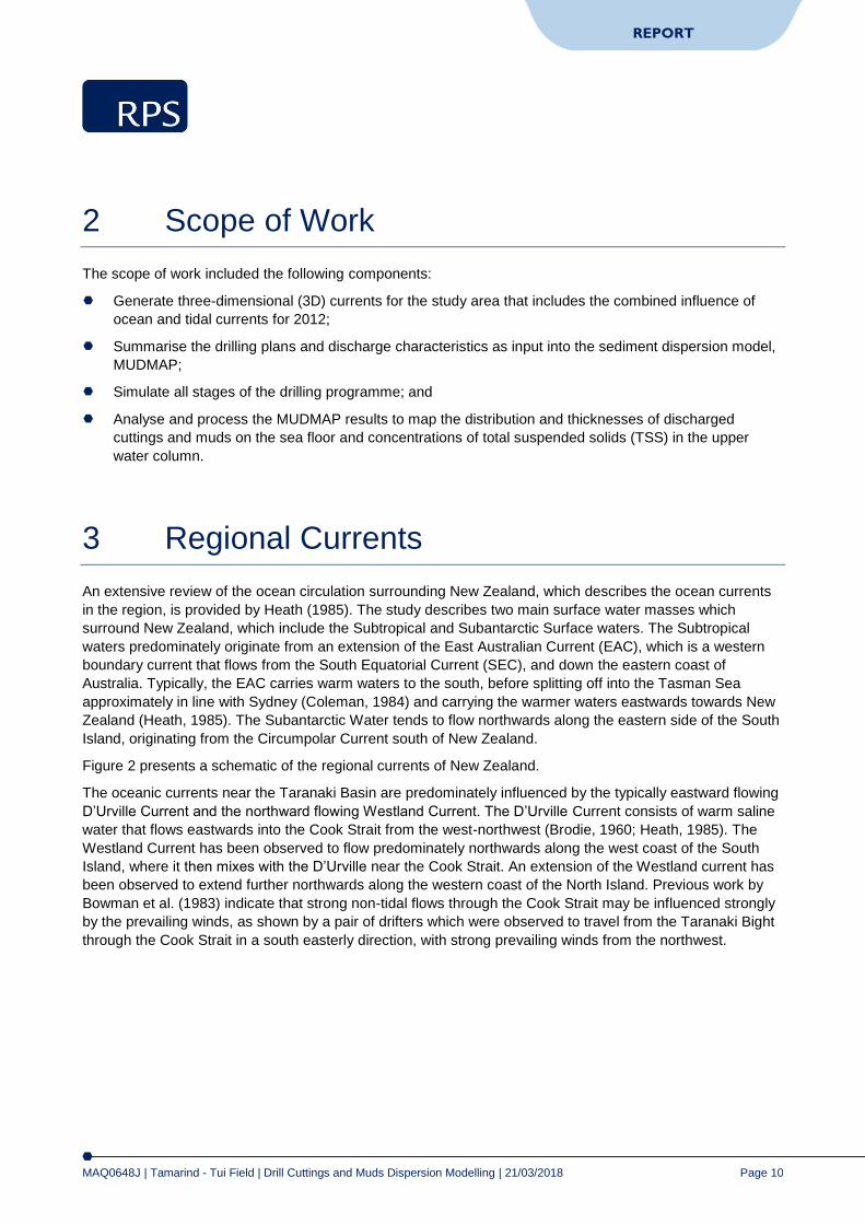
Figure 2 presents a schematic of the regional currents of New Zealand.

The oceanic currents near the Taranaki Basin are predominately influenced by the typically eastward flowing D’Urville Current and the northward flowing Westland Current. The D’Urville Current consists of warm saline water that flows eastwards into the Cook Strait from the west-northwest (Brodie, 1960; Heath, 1985). The Westland Current has been observed to flow predominately northwards along the west coast of the South Island, where it then mixes with the D’Urville near the Cook Strait. An extension of the Westland current has been observed to extend further northwards along the western coast of the North Island. Previous work by Bowman et al. (1983) indicate that strong non-tidal flows through the Cook Strait may be influenced strongly by the prevailing winds, as shown by a pair of drifters which were observed to travel from the Taranaki Bight through the Cook Strait in a south easterly direction, with strong prevailing winds from the northwest.


Page 11

REPORT

Figure 2 Schematic showing the oceanic current circulation surrounding New Zealand (Image source: Brodie, 1960).


Page 12

REPORT

3.1Tidal Currents The effects of tides were generated using RPS’s advanced ocean/coastal model, HYDROMAP. The

HYDROMAP model has been thoroughly tested and verified through field measurements throughout the world over more than 20 years (Isaji and Spaulding, 1984; Isaji et al., 2001; Zigic et al., 2003). In fact, HYDROMAP tidal current data has been used as input for the OILMAP hydrocarbon spill modelling system, which forms part of the Incident Management System (IMS) operated by Maritime New Zealand (MNZ).

HYDROMAP employs a sophisticated sub-gridding strategy, which supports up to six levels of spatial resolution, halving the grid cell size as each level of resolution is employed. The sub-gridding allows for higher resolution of currents within areas of greater bathymetric and coastline complexity, and/or of particular interest to a study.

The numerical solution methodology follows that of Davies (1977a and 1977b) with further developments for model efficiency by Owen (1980) and Gordon (1982). A more detailed presentation of the model can be found in Isaji and Spaulding (1984) and Isaji et al. (2001).

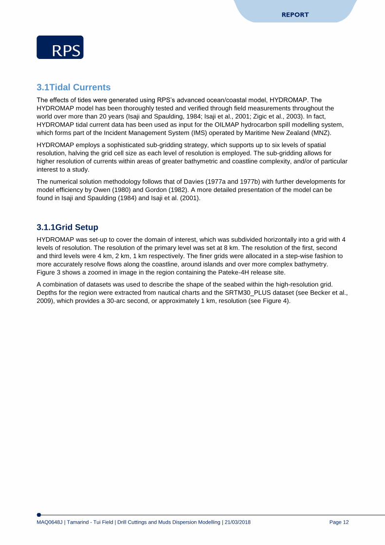
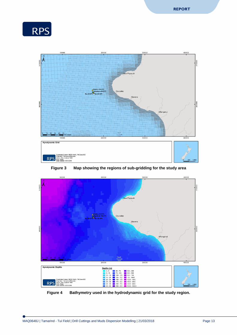
3.1.1Grid Setup HYDROMAP was set-up to cover the domain of interest, which was subdivided horizontally into a grid with 4 levels of resolution. The resolution of the primary level was set at 8 km. The resolution of the first, second and third levels were 4 km, 2 km, 1 km respectively. The finer grids were allocated in a step-wise fashion to more accurately resolve flows along the coastline, around islands and over more complex bathymetry. Figure 3 shows a zoomed in image in the region containing the Pateke-4H release site.

A combination of datasets was used to describe the shape of the seabed within the high-resolution grid. Depths for the region were extracted from nautical charts and the SRTM30_PLUS dataset (see Becker et al., 2009), which provides a 30-arc second, or approximately 1 km, resolution (see Figure 4).


Page 13

REPORT

Figure 3 Map showing the regions of sub-gridding for the study area

Figure 4 Bathymetry used in the hydrodynamic grid for the study region.

MAQ0648J | Tamarind - Tui Field | Drill Cuttings and Muds Dispersion Modelling | 21/03/2018 Page 14

REPORT

3.1.2 Tidal Conditions

The ocean boundary data for the regional model was obtained from satellite measured altimetry data (TOPEX/Poseidon 7.2) which provided estimates of the eight dominant tidal constituents at a horizontal scale of approximately 0.25 degrees. The eight major tidal constituents used were K2, S2, M2, N2, K1, P1, O1 and Q1. Using the tidal data, surface heights were firstly calculated along the open boundaries, at each time step in the model.

The Topex-Poseidon satellite data is produced, and quality controlled by National Aeronautics and Space Administration (NASA). The satellites, equipped with two highly accurate altimeters, capable of taking sea level measurements accurate to less than ± 5 cm, measured oceanic surface elevations (and the resultant tides) for over 13 years (1992–2005). In total these satellites carried out 62,000 orbits of the planet. The Topex-Poseidon tidal data has been widely used amongst the oceanographic community, being the subject of more than 2,100 research publications (e.g. Andersen, 1995; Ludicone et al., 1998; Matsumoto et al., 2000; Kostianoy et al., 2003; Yaremchuk and Tangdong, 2004; Qiu and Chen 2010). As such the Topex/Poseidon tidal data is considered suitably accurate for this study.

3.1.3 Surface Elevation Validation

To ensure that tidal predictions were accurate, predicted surface elevations were compared to data observed at five locations situated across the study region (Figure 5).

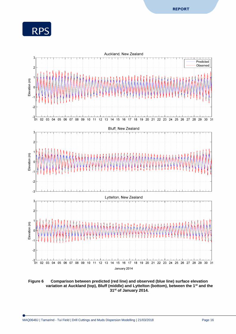
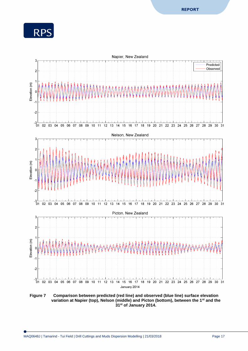
Figure 6 to Figure 8 illustrate a comparison of the predicted and observed surface elevations for each location for January 2014. As shown on the graph, the model accurately reproduced the phase and amplitudes throughout the spring and neap tidal cycles.

To provide a statistical measure of the model’s performance, the Index of Agreement (IOA – Willmott, 1981) and the Mean Absolute Error (MAE – Willmott, 1982; Willmott and Matsuura, 2005) were used.

The MAE is the average of the absolute values of the difference between the model-predicted (P) and observed (O) variables. It is a more natural measure of the average error and more readily understood (Willmott and Matsuura, 2005).

𝑀𝐴𝐸 = 𝑁−1∑|𝑃𝑖 − 𝑂𝑖|

𝑁

𝑖=1

The Index of Agreement (IOA) is determined by:

𝐼𝑂𝐴 = 1 −∑|𝑋𝑚𝑜𝑑𝑒𝑙 − 𝑋𝑜𝑏𝑠|

2

∑(|𝑋𝑚𝑜𝑑𝑒𝑙 − 𝑋𝑜𝑏𝑠̅̅ ̅̅ ̅̅ | + |𝑋𝑜𝑏𝑠 − 𝑋𝑜𝑏𝑠̅̅ ̅̅ ̅̅ |)2

Where: X represents the variable being compared and the time mean of that variable. A perfect agreement exists between the model and field observations if the index gives an agreement value of 1 and complete disagreement will produce an index measure of 0 (Willmott, 1981). Willmott et al., (1985) also suggests that values meaningfully larger than 0.5 represent good model performance. Clearly, a greater IOA and lower MAE represent a better model performance.

Table 2 shows the IOA and MAE values for the selected locations.


Page 15

REPORT

Figure 5 Location of the nine tide stations around New Zealand used to validate the tidal model.

Table 2 Statistical comparison between the observed and HYDROMAP predicted surface elevations data from the 1st to 31st January 2014.

Tide Station IOA MAE (m)

Auckland (North Island) 0.95 0.29

Bluff (South Island) 0.93 0.25

Lyttelton (South Island) 0.91 0.26

Napier (North Island) 0.98 0.11

Nelson (South Island) 0.93 0.39

Picton (South Island) 0.93 0.15

Port Taranaki (North Island) 0.94 0.33

Wellington (North Island) 0.95 0.13

Westport (South Island) 0.94 0.30

Average 0.94 0.25


Page 16

REPORT

Figure 6 Comparison between predicted (red line) and observed (blue line) surface elevation variation at Auckland (top), Bluff (middle) and Lyttelton (bottom), between the 1st and the

31st of January 2014.


Page 17

REPORT

Figure 7 Comparison between predicted (red line) and observed (blue line) surface elevation variation at Napier (top), Nelson (middle) and Picton (bottom), between the 1st and the

31st of January 2014.


Page 18

REPORT

Figure 8 Comparison between predicted (red line) and observed (blue line) surface elevation variation at Port Taranaki (top), Wellington (middle) and Westport (bottom), between the

1st and 31st of January 2014.


Page 19

REPORT

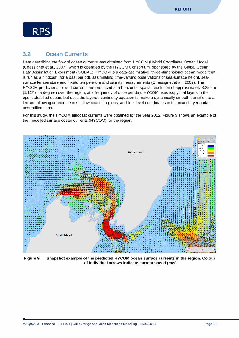
3.2 Ocean Currents Data describing the flow of ocean currents was obtained from HYCOM (Hybrid Coordinate Ocean Model, (Chassignet et al., 2007), which is operated by the HYCOM Consortium, sponsored by the Global Ocean Data Assimilation Experiment (GODAE). HYCOM is a data-assimilative, three-dimensional ocean model that is run as a hindcast (for a past period), assimilating time-varying observations of sea-surface height, sea-surface temperature and in-situ temperature and salinity measurements (Chassignet et al., 2009). The HYCOM predictions for drift currents are produced at a horizontal spatial resolution of approximately 8.25 km (1/12th of a degree) over the region, at a frequency of once per day. HYCOM uses isopycnal layers in the open, stratified ocean, but uses the layered continuity equation to make a dynamically smooth transition to a terrainfollowing coordinate in shallow coastal regions, and to zlevel coordinates in the mixed layer and/or unstratified seas.

For this study, the HYCOM hindcast currents were obtained for the year 2012. Figure 9 shows an example of the modelled surface ocean currents (HYCOM) for the region.

Figure 9 Snapshot example of the predicted HYCOM ocean surface currents in the region. Colour of individual arrows indicate current speed (m/s).


Page 20

REPORT

3.3 Currents at the Release Site Table 3 displays the average and maximum combined surface current speeds (ocean plus tides) nearby the release sites. Figure 10 shows the monthly surface current rose distributions nearby the release sites.

Note the convention for defining current direction is the direction the current flows towards, which is used to reference current direction throughout this report. Each branch of the rose represents the currents flowing to that direction, with north to the top of the diagram. Sixteen directions are used. The branches are divided into segments of different colour, which represent the current speed ranges for each direction. Speed intervals of 0.1 m/s are typically used in these current roses. The length of each coloured segment is relative to the proportion of currents flowing within the corresponding speed and direction.

The data showed that the surface current speeds and directions were variable between the months, though with a predominant flow towards the south-southeast and north. The maximum and average surface current speeds were 1.44 m/s 0.24 m/s, respectively.

Table 3 Predicted average and maximum surface current speeds at the study site. The data was derived by combining the HYCOM ocean data and HYDROMAP tidal data for 2008-2012

(inclusive).

Month Average current

speed (m/s) Maximum current

speed (m/s) General Direction

January 0.24 1.17 Northeast to Southeast

February 0.20 0.96 Northeast to Southeast

March 0.23 1.37 Northwest and Southeast

April 0.25 1.44 Southeast

May 0.26 0.91 Southeast

June 0.25 1.04 Variable

July 0.24 1.10 Northwest to Northeast

August 0.23 1.21 South

September 0.27 1.32 Southeast

October 0.25 1.00 Northeast to southeast

November 0.23 1.07 Northeast

December 0.25 0.94 Southeast

Minimum 0.20 0.91

Maximum 0.27 1.44


Page 21

REPORT

Figure 10 Predicted monthly surface current rose plots at the study site. Data was derived by combining the HYDROMAP tidal currents and HYCOM ocean currents for 2008 – 2012.

The colour key shows the current speed (m/s), the compass direction provides the current direction flowing TOWARDS and the length of the wedge gives the percentage of

the record for a particular speed and direction combination.


Page 22

REPORT

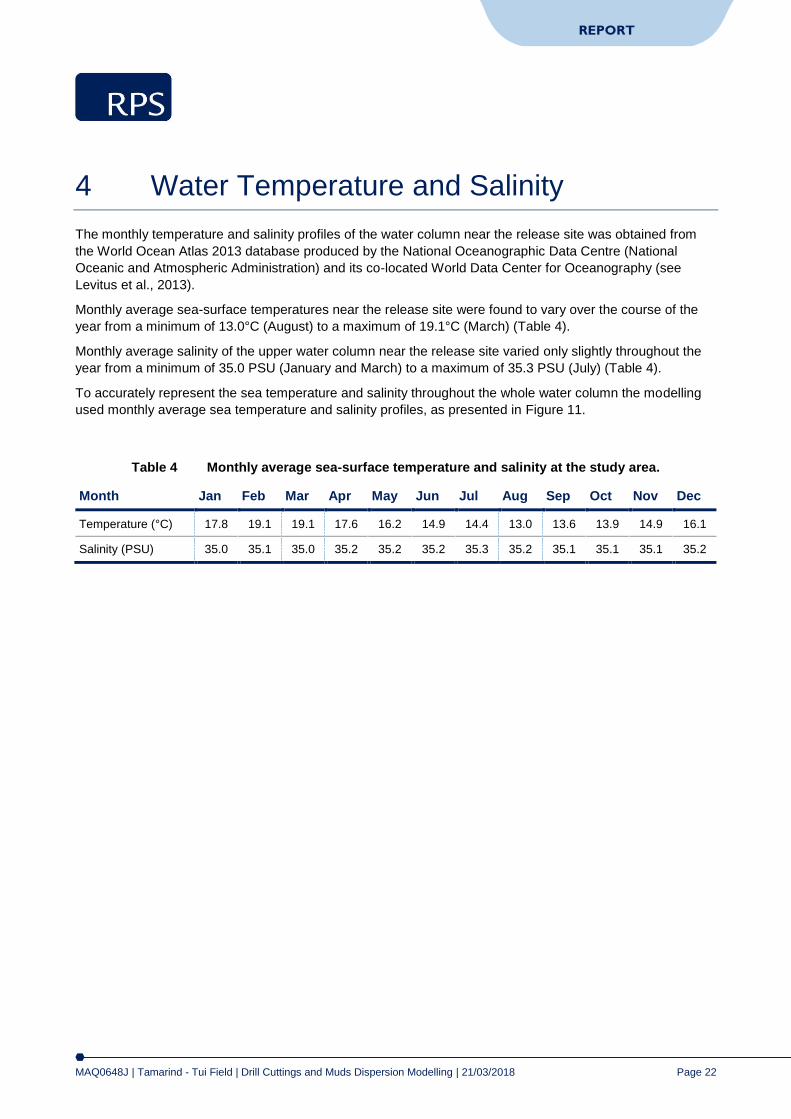
4 Water Temperature and Salinity

The monthly temperature and salinity profiles of the water column near the release site was obtained from the World Ocean Atlas 2013 database produced by the National Oceanographic Data Centre (National Oceanic and Atmospheric Administration) and its co-located World Data Center for Oceanography (see Levitus et al., 2013).

Monthly average sea-surface temperatures near the release site were found to vary over the course of the year from a minimum of 13.0°C (August) to a maximum of 19.1°C (March) (Table 4).

Monthly average salinity of the upper water column near the release site varied only slightly throughout the year from a minimum of 35.0 PSU (January and March) to a maximum of 35.3 PSU (July) (Table 4).

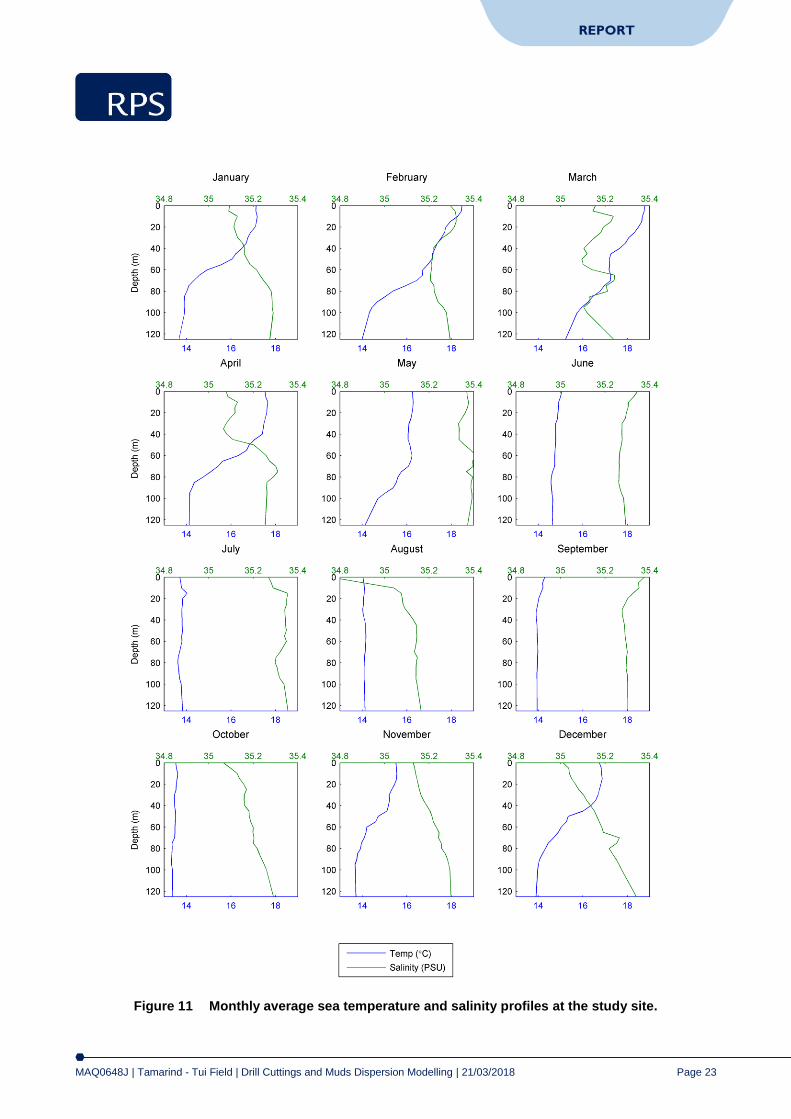
To accurately represent the sea temperature and salinity throughout the whole water column the modelling used monthly average sea temperature and salinity profiles, as presented in Figure 11.

Table 4 Monthly average sea-surface temperature and salinity at the study area.

Month Jan Feb Mar Apr May Jun Jul Aug Sep Oct Nov Dec

Temperature (°C) 17.8 19.1 19.1 17.6 16.2 14.9 14.4 13.0 13.6 13.9 14.9 16.1

Salinity (PSU) 35.0 35.1 35.0 35.2 35.2 35.2 35.3 35.2 35.1 35.1 35.1 35.2


Page 23

REPORT

Figure 11 Monthly average sea temperature and salinity profiles at the study site.


Page 24

REPORT

5 Sediment Dispersion Modelling

5.1 Model Description - MUDMAP MUDMAP is a three-dimensional plume model used by industry and regulators to aid in assessing the potential environmental effects from operational discharges such as drill cuttings, drilling fluids and produced water. The model has been applied to hundreds of assessments in over 35 countries, including New Zealand.

The model itself is an enhancement of the Offshore Operators Committee (OOC) model and calculates the fates of discharges through three distinct stages, as defined by laboratory and field studies (Koh and Chang 1973; Khondaker 2000):

Stage 1: Convective descent – free fall of the combined mass of fluids and cuttings;

Stage 2: Dynamic collapse stage – the collapse of the combined mass as it meets the seabed (or water surface);

Stage 3: Dispersion stage – the transport and dispersion of discharged fluids and particles by the local currents. For cuttings and drilling mud particles that have higher density than seawater, this phase also calculates sinking and settlement to the seabed.

Each stage plays an integral role on different time and distance scales. The governing equations and solutions of MUDMAP were built on the formulas originally developed by Koh and Chang (1973) and are extended by the work of Brandsma and Sauer (1983), known as the OOC model, for Stages 1 and 2 of plume motion.

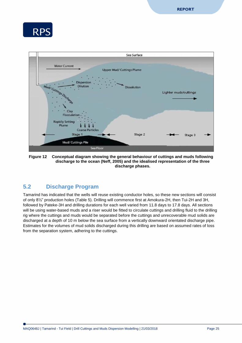
The far-field calculation (passive dispersion stage), employs a particle-based, random walk procedure. The model predicts the dynamics of the discharge material and resulting seabed concentrations and bottom thicknesses over the near-field (i.e. the immediate area of the discharge) and the far-field (the wider region). Figure 12 shows a conceptual diagram of the dispersion and fates of drill cuttings and fluids discharge to the ocean and an idealized representation of the three discharge phases.

Settling under currents is selective for particle size, with the larger particles (rock chips to sand) tending to settle quickly, forming a pile that aligns with the predominant current axis. Smaller particles (especially silts and clays) will remain suspended for longer periods and will therefore be dispersed more widely by the ambient current conditions. Dispersion of the finer discharged material will tend to be enhanced with increased current speeds and water depth and with greater variation in current direction over time and depth.

Along with the advanced analyses tools, MUDMAP can simulate six classes of material (with up to 36 sub-categories), each with unique density and particle-size distribution. During the dispersion stage, the model particles are transported in three-dimensions according to the current data and horizontal and vertical mixing coefficients at each time step according to the governing equations.

MUDMAP has been extensively validated and applied for discharge operations in Australian coastal waters (e.g. Burns et. al. 1999; King and McAllister 1997, 1998; Spaulding, 1994).


Page 25

REPORT

Figure 12 Conceptual diagram showing the general behaviour of cuttings and muds following discharge to the ocean (Neff, 2005) and the idealised representation of the three

discharge phases.

5.2 Discharge Program Tamarind has indicated that the wells will reuse existing conductor holes, so these new sections will consist of only 8½” production holes (Table 5). Drilling will commence first at Amokura-2H, then Tui-2H and 3H, followed by Pateke-3H and drilling durations for each well varied from 11.8 days to 17.8 days. All sections will be using water-based muds and a riser would be fitted to circulate cuttings and drilling fluid to the drilling rig where the cuttings and muds would be separated before the cuttings and unrecoverable mud solids are discharged at a depth of 10 m below the sea surface from a vertically downward orientated discharge pipe. Estimates for the volumes of mud solids discharged during this drilling are based on assumed rates of loss from the separation system, adhering to the cuttings.


Page 26

REPORT

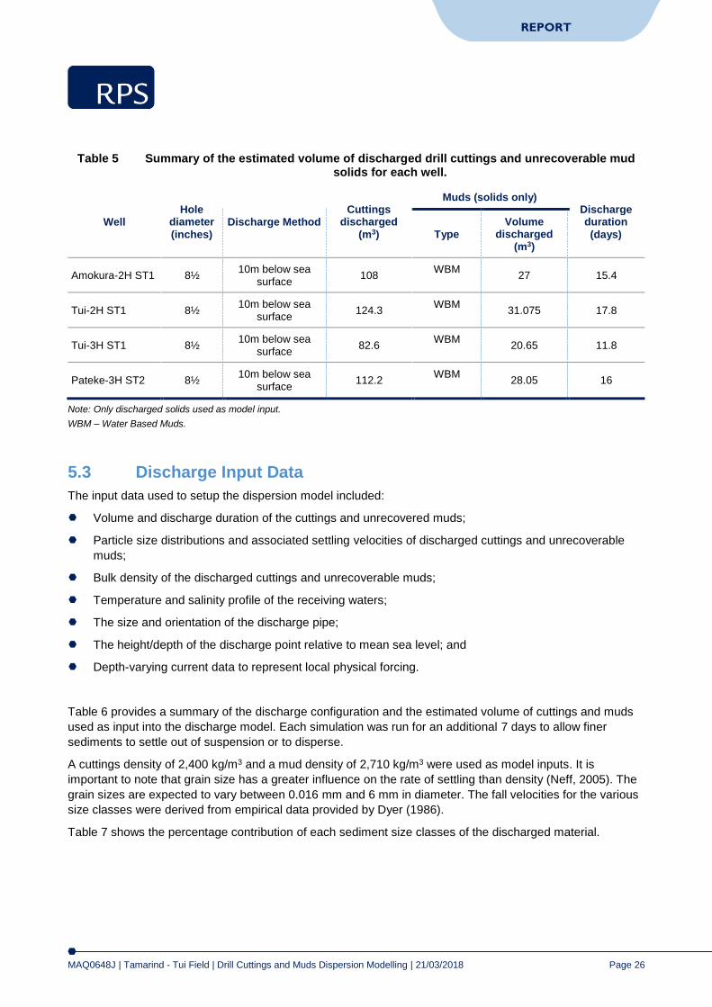
Table 5 Summary of the estimated volume of discharged drill cuttings and unrecoverable mud solids for each well.

Well Hole

diameter (inches)

Discharge Method Cuttings

discharged (m3)

Muds (solids only) Discharge duration (days) Type

Volume discharged

(m3)

Amokura-2H ST1 8½ 10m below sea

surface 108

WBM 27 15.4

Tui-2H ST1 8½ 10m below sea

surface 124.3

WBM 31.075 17.8

Tui-3H ST1 8½ 10m below sea

surface 82.6

WBM 20.65 11.8

Pateke-3H ST2 8½ 10m below sea

surface 112.2

WBM 28.05 16

Note: Only discharged solids used as model input.

WBM – Water Based Muds.

5.3 Discharge Input Data The input data used to setup the dispersion model included:

Volume and discharge duration of the cuttings and unrecovered muds;

Particle size distributions and associated settling velocities of discharged cuttings and unrecoverable muds;

Bulk density of the discharged cuttings and unrecoverable muds;

Temperature and salinity profile of the receiving waters;

The size and orientation of the discharge pipe;

The height/depth of the discharge point relative to mean sea level; and

Depth-varying current data to represent local physical forcing.

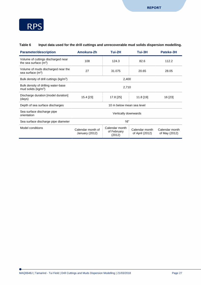
Table 6 provides a summary of the discharge configuration and the estimated volume of cuttings and muds used as input into the discharge model. Each simulation was run for an additional 7 days to allow finer sediments to settle out of suspension or to disperse.

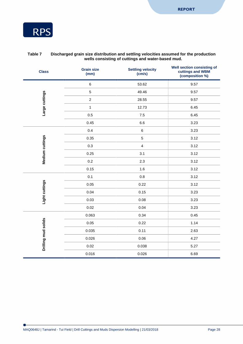
A cuttings density of 2,400 kg/m3 and a mud density of 2,710 kg/m3 were used as model inputs. It is important to note that grain size has a greater influence on the rate of settling than density (Neff, 2005). The grain sizes are expected to vary between 0.016 mm and 6 mm in diameter. The fall velocities for the various size classes were derived from empirical data provided by Dyer (1986).

Table 7 shows the percentage contribution of each sediment size classes of the discharged material.


Page 27

REPORT

Table 6 Input data used for the drill cuttings and unrecoverable mud solids dispersion modelling.

Parameter/description Amokura-2h Tui-2H Tui-3H Pateke-3H

Volume of cuttings discharged near the sea surface (m3)

108 124.3 82.6 112.2

Volume of muds discharged near the sea surface (m3)

27 31.075 20.65 28.05

Bulk density of drill cuttings (kg/m3) 2,400

Bulk density of drilling water-base mud solids (kg/m3)

2,710

Discharge duration [model duration] (days)

15.4 [23] 17.8 [25] 11.8 [19] 16 [23]

Depth of sea surface discharges 10 m below mean sea level

Sea surface discharge pipe orientation

Vertically downwards

Sea surface discharge pipe diameter 16”

Model conditions Calendar month of

January (2012)

Calendar month of February

(2012)

Calendar month of April (2012)

Calendar month of May (2012)


Page 28

REPORT

Table 7 Discharged grain size distribution and settling velocities assumed for the production wells consisting of cuttings and water-based mud.

Class Grain size

(mm) Settling velocity

(cm/s)

Well section consisting of cuttings and WBM (composition %)

La

rge

cu

ttin

gs

6 53.62 9.57

5 49.46 9.57

2 28.55 9.57

1 12.73 6.45

0.5 7.5 6.45

0.45 6.6 3.23

Me

diu

m c

utt

ing

s

0.4 6 3.23

0.35 5 3.12

0.3 4 3.12

0.25 3.1 3.12

0.2 2.3 3.12

0.15 1.6 3.12

Lig

ht

cu

ttin

gs

0.1 0.8 3.12

0.05 0.22 3.12

0.04 0.15 3.23

0.03 0.08 3.23

0.02 0.04 3.23

Dri

llin

g m

ud

so

lids

0.063 0.34 0.45

0.05 0.22 1.14

0.035 0.11 2.63

0.026 0.06 4.27

0.02 0.038 5.27

0.016 0.026 6.69


Page 29

REPORT

5.4 Grid Configuration A grid covering a 20 km (longitude, x-direction) by 20 km (latitude, y-direction) region with each grid cell being 20 m (x) x 20 m (y) was employed to calculate the thickness of deposited drill cuttings and muds on the seafloor, with vertical divisions of 10 m to allow for assessing total suspended solids in the water column.

5.5 Mixing Parameters A horizontal coefficient value of 0.1 m2/s and a vertical coefficient value of 0.01 m2/s was applied to account for turbulent mixing processes that occur as the discharged material disperses from the near-surface release point.

5.6 Minimum Reporting Thresholds As the MUDMAP model has the ability to track cuttings and muds to thicknesses (and concentrations) that are lower than biologically significant, it was necessary to specify a minimum reporting threshold for the predicted bottom thickness which would record the “exposure” on the seafloor above natural sedimentation rates.

The threshold adopted for sea floor deposition was calculated using a conservatively assumed background sedimentation rate of 10 g/m2/day. This sedimentation rate, multiplied by 40 days, which is the average time to complete each well, provides a deposition threshold of 400 g/m2. This deposition threshold was converted to a minimum thickness by considering the average bulk density of the cuttings and mud solids. To account for voids within the newly settled cuttings and muds a bulking factor of 2.5 was applied to give a final minimum deposition thickness threshold of 0.4 mm (or 400 µm). This same bulking factor was applied to the modelling results.

Total suspended solids (TSS) thresholds were set to a conservative level of 1 mg/l.


Page 30

REPORT

6 Results

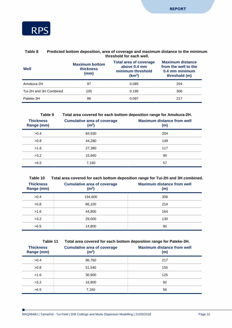
Table 8 to Table 11 provide a summary of deposition on the sea floor for each well, above the minimum threshold of 0.4 mm (400 µm), while Figure 13 to Figure 15 show the spatial distributions of the sea floor deposition.

Maximum thickness on the sea floor ranged from 86 mm for the Pateke-3H well to 105 mm for the combined Tui wells. These maximum thicknesses occurred within 20 meters of the well.

Sea floor deposition greater than the 0.4 mm threshold reached maximum distances ranging from 204 m for the Amokura-2H well to 306 m for the combined Tui wells.

The maximum areas of sea floor coverage above the minimum threshold of 0.4 mm ranged from 84,930 m2 (0.085 km2) for the Amokura-2H well to 194,600 m2 (0.195 km2) for the combined Tui wells.

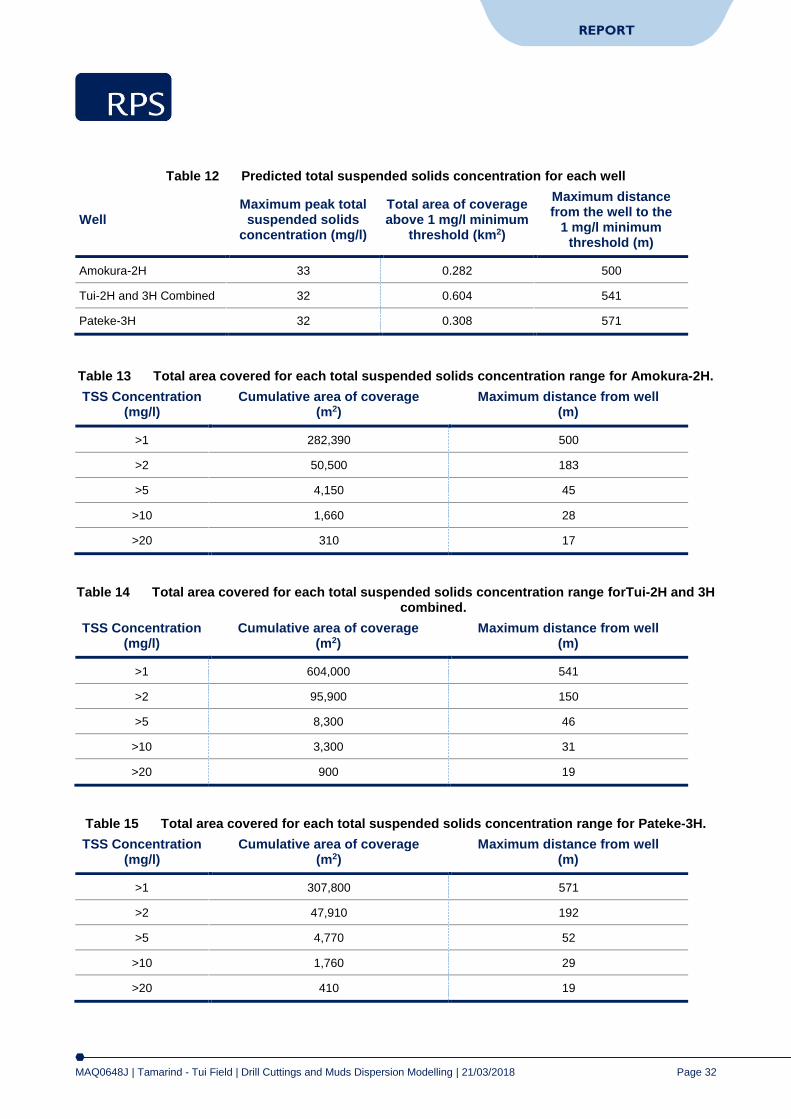
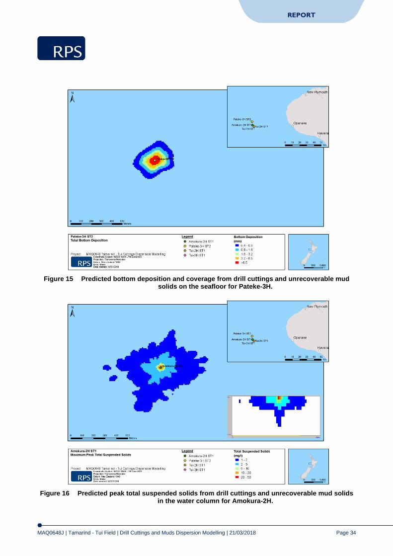
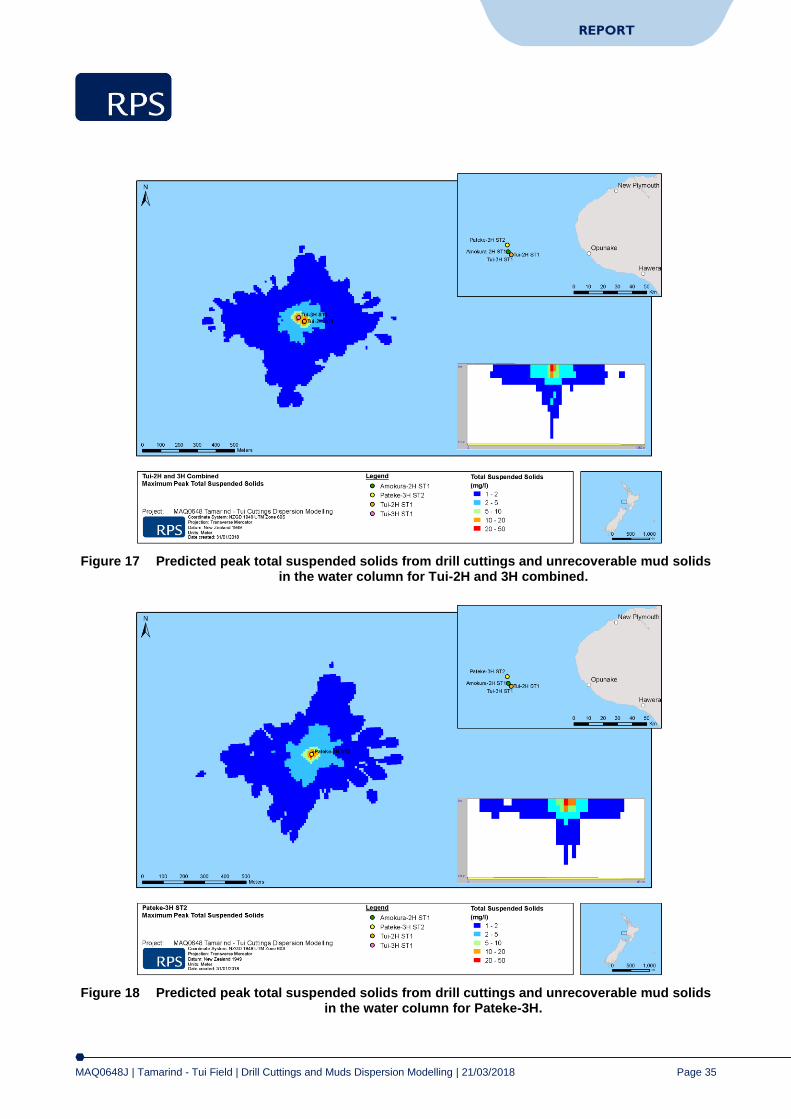
Table 12 to Table 15 provide a summary of peak TSS concentrations in the water column for each well, above the minim um threshold of 1 mg/l, while Figure 16 to Figure 18 show the spatial distributions of the in-water TSS along with a cross-section to demonstrate the depth of penetration..

Peak TSS values at the well sites were consistent, with a maximum of 33 mg/l.

Maximum peak TSS values greater than the 1 mg/l threshold reached maximum distances ranging from 500 m for the Amokura-2H well to 571 m for the Pateke-3H well.

The total areas of influence by TSS values greater than the threshold of 1 mg/l ranged from 282,390 m2 (0.282 km2) for the Amokura-2H well to 604,000 m2 (0.604 km2) for the combined Tui wells.

TSS concentrations of 10 mg/l were only observed in the top 20 m of the water column, while TSS concentrations down to 2 mg/l were only observed down to 30 or 40 m.

TSS concentrations greater than 1 mg/l extended almost all the way to the seabed directly under the discharge site, due to material falling through this column of water, however further afield TSS concentrations greater than 1 mg/l were only observed in the top 30 to 40 m of the water column.


Page 31

REPORT

Table 8 Predicted bottom deposition, area of coverage and maximum distance to the minimum threshold for each well.

Well Maximum bottom

thickness (mm)

Total area of coverage above 0.4 mm

minimum threshold (km2)

Maximum distance from the well to the 0.4 mm minimum

threshold (m)

Amokura-2H 97 0.085 204

Tui-2H and 3H Combined 105 0.195 306

Pateke-3H 86 0.097 217

Table 9 Total area covered for each bottom deposition range for Amokura-2H.

Thickness Range (mm)

Cumulative area of coverage (m2)

Maximum distance from well (m)

>0.4 84,930 204

>0.8 44,280 149

>1.6 27,380 117

>3.2 15,660 90

>6.5 7,160 57

Table 10 Total area covered for each bottom deposition range for Tui-2H and 3H combined.




>0.4 194,600 306

>0.8 86,100 214

>1.6 44,800 164

>3.2 29,000 130

>6.5 14,800 90

Table 11 Total area covered for each bottom deposition range for Pateke-3H.




>0.4 96,760 217

>0.8 51,540 155

>1.6 30,900 125

>3.2 16,800 92

>6.5 7,160 56


Page 32

REPORT

Table 12 Predicted total suspended solids concentration for each well

Well Maximum peak total

suspended solids concentration (mg/l)

Total area of coverage above 1 mg/l minimum

threshold (km2)

Maximum distance from the well to the

1 mg/l minimum threshold (m)

Amokura-2H 33 0.282 500

Tui-2H and 3H Combined 32 0.604 541

Pateke-3H 32 0.308 571

Table 13 Total area covered for each total suspended solids concentration range for Amokura-2H.

TSS Concentration (mg/l)



>1 282,390 500

>2 50,500 183

>5 4,150 45

>10 1,660 28

>20 310 17

Table 14 Total area covered for each total suspended solids concentration range forTui-2H and 3H combined.




>1 604,000 541

>2 95,900 150

>5 8,300 46

>10 3,300 31

>20 900 19

Table 15 Total area covered for each total suspended solids concentration range for Pateke-3H.




>1 307,800 571

>2 47,910 192

>5 4,770 52

>10 1,760 29

>20 410 19


Page 33

REPORT

Figure 13 Predicted bottom deposition and coverage from drill cuttings and unrecoverable mud solids on the seafloor for Amokura-2H.

Figure 14 Predicted bottom deposition and coverage from drill cuttings and unrecoverable mud solids on the seafloor for Tui-2H and 3H combined.


Page 34

REPORT

Figure 15 Predicted bottom deposition and coverage from drill cuttings and unrecoverable mud solids on the seafloor for Pateke-3H.

Figure 16 Predicted peak total suspended solids from drill cuttings and unrecoverable mud solids in the water column for Amokura-2H.


Page 35

REPORT

Figure 17 Predicted peak total suspended solids from drill cuttings and unrecoverable mud solids in the water column for Tui-2H and 3H combined.

Figure 18 Predicted peak total suspended solids from drill cuttings and unrecoverable mud solids in the water column for Pateke-3H.


Page 36

REPORT

7 References

Andersen, OB 1995, ‘Global ocean tides from ERS 1 and TOPEX/POSEIDON altimetry’, Journal of

Geophysical Research: Oceans, vol. 100, no. C12, pp. 25249–25259.

Becker, JJ, Sandwell, DT, Smith, WHF, Braud, J, Binder, B, Depner, J, Fabre, D, Factor, J, Ingalls, S, Kim, S-H, Ladner, R, Marks, K, Nelson, S, Pharaoh, A, Trimmer, R, Von Rosenberg, J, Wallace, G & Weatherall, P 2009, ‘Global bathymetry and evaluation data at 30 arc seconds resolution: SRTM30_PLUS’, Marine Geodesy, vol. 32, no. 4, pp. 355–371.

Bowman, MJ, Kibblewhite, AC, Murtagh, RA, Chiswell, SM & Sandersin, BG 1983, ‘Circulation and mixing in greater Cook Straight, New Zealand’, Oceanologica Acta, vol. 6, no. 4, pp. 383–391.

Brandsma, MG & Sauer Jr, TC 1983. ‘The OOC model: prediction of short term fate of drilling mud in the

ocean, Part I model description and Part II model results’, Proceedings of Workshop on An Evaluation

of Effluent Dispersion and Fate Models for OCS Platforms, Minerals Management Service, Santa Barbara, pp. 86–106.

Brodie, JW 1960, ‘Coastal surface currents around New Zealand’, New Zealand Journal of Geology and

Geophysics, vol. 3, no. 2, pp. 235–252.

Burns, K, Codi, S, Furnas, M, Heggie, D, Holdway, D, King, B, & McAllister, F 1999, ‘Dispersion and Fate of

Produced Formation Water Constituents in an Australian Northwest Shelf Shallow Water Ecosystem’,

Marine Pollution Bulletin, vol. 38, no. 7, pp. 593–603.

Chassignet, EP, Hurlburt, HE, Smedstad, OM, Halliwell, GR, Hogan, PJ, Wallcraft, AJ, Baraille, R & Bleck, R 2007, ‘The HYCOM (hybrid coordinate ocean model) data assimilative system’, Journal of Marine

Systems, vol. 65, no. 1, pp. 60–83.

Chassignet, E, Hurlburt, H, Metzger, E, Smedstad, O, Cummings, J & Halliwell, G 2009, ‘U.S. GODAE:

Global Ocean Prediction with the HYbrid Coordinate Ocean Model (HYCOM)’, Oceanography, vol. 22,

no. 2, pp. 64–75.

Coleman, R 1984, ‘Investigation of the Tasman Sea by satellite altimetry’, Australian Journal of Marine and

Freshwater Research, vol. 35, no. 6, pp. 619–633.

Davies, AM 1977a, ‘The numerical solutions of the three-dimensional hydrodynamic equations using a B-spline representation of the vertical current profile’, in JC Nihoul (ed), Bottom Turbulence: Proceedings of the 8th Liège Colloquium on Ocean Hydrodynamics, Elsevier Scientific, Amsterdam, pp. 1–25.

Davies, AM 1977b, ‘Three-dimensional model with depth-varying eddy viscosity’, in JC Nihoul (ed), Bottom

Turbulence: Proceedings of the 8th Liège Colloquium on Ocean Hydrodynamics, Elsevier Scientific, Amsterdam, pp. 27–48.

Dyer, KR 1986, Coastal and Estuarine Sediment Dynamics, John Wiley & Sons Ltd., Chichester.

Gordon, R 1982, Wind driven circulation in Narragansett Bay, Doctor of philosophy thesis, University of Rhode Island, Kingston.


Page 37

REPORT

Heath, RA 1985, ‘Large-scale influence of the New Zealand seafloor topography on western boundary currents of the South Pacific Ocean’, Australian Journal of Marine and Freshwater Research, vol. 36, no. 1, pp. 1–14.

Isaji, T & Spaulding, M 1984, ‘A model of the tidally induced residual circulation in the Gulf of Maine and

Georges Bank’, Journal of Physical Oceanography, vol. 14, no. 6, pp. 1119–1126.

Isaji, T, Howlett, E, Dalton C, & Anderson, E 2001, ‘Stepwise-continuous-variable-rectangular grid hydrodynamics model’, Proceedings of the 24th Arctic and Marine Oil spill Program (AMOP) Technical

Seminar (including 18th TSOCS and 3rd PHYTO), Environment Canada, Edmonton, pp. 597–610.

Khondaker, AN 2000, ‘Modeling the fate of drilling waste in marine environment – an overview’, Journal of

Computers and Geosciences, vol. 26, no. 5, pp. 531–540.

King, B & McAllister, FA 1997, Modelling the Dispersion of Produced Water Discharge in Australia 1 & 2. Australian Institute of Marine Science, Townsville.

King, B & McAllister, FA 1998, ‘Modelling the dispersion of produced water discharges’, APPEA Journal, pp. 681–691.

Koh, RCY & Chang, YC 1973. Mathematical model for barged ocean disposal of waste, U.S. Army Engineer Waterways Experiment Station, Vicksburg.

Kostianoy, AG, Ginzburg, AI, Lebedev, SA, Frankignoulle, M & Delille, B 2003, ‘Fronts and mesoscale

variability in the southern Indian Ocean as inferred from the TOPEX/POSEIDON and ERS-2 Altimetry data’, Oceanology, vol. 43, no. 5, pp. 632–642.

Levitus, S, Antonov, JI, Baranova, OK, Boyer, TP, Coleman, CL, Garcia, HE, Grodsky, AI, Johnson, DR, Locarnini, RA, Mishonov, AV, Reagan, JR, Sazama, CL, Seidov, D, Smolyar, I, Yarosh, ES & Zweng, MM 2013, ‘The World Ocean Database’, Data Science Journal, vol. 12, no. 0, pp. WDS229–WDS234.

Ludicone, D, Santoleri, R, Marullo, S & Gerosa, P 1998, ‘Sea level variability and surface eddy statistics in

the Mediterranean Sea from TOPEX/POSEIDON data’, Journal of Geophysical Research I, vol. 103, no. C2, pp. 2995–3011.

Matsumoto, K, Takanezawa, T & Ooe, M 2000, ‘Ocean tide models developed by assimilating

TOPEX/POSEIDON altimeter data into hydrodynamical model: A global model and a regional model around Japan’, Journal of Oceanography, vol. 56, no.5, pp. 567–581.

Neff, J 2005, Composition, environment fates, and biological effect of water based drilling fluids and cuttings

discharged to the marine environment: A synthesis and annotated bibliography, Battelle, Duxbury.

Owen, A., 1980, ‘A three-dimensional model of the Bristol Channel’, Journal of Physical Oceanography, vol. 10, no. 8, pp. 1290–1302.

Qiu, B & Chen, S 2010, ‘Eddy-mean flow interaction in the decadally modulating Kuroshio Extension system’, Deep-Sea Research II, vol. 57, no. 13, 1098–1110.

Spaulding, ML 1994, ‘Drilling, production fluids dispersion predicted by model’, Offshore, vol. 54, no. 4, pp. 78–82.


Page 38

REPORT

Willmott, CJ 1981, ‘On the validation of models’, Physical Geography, vol. 2, no. 2, pp. 184–194.

Willmott, CJ 1982, ‘Some comments on the evaluation of model performance’, Bulletin of the American

Meteorological Society, vol. 63, no. 11, pp. 1309–1313.

Willmott CJ, Ackleson SG, Davis RE, Feddema JJ, Klink, KM, Legates, DR, O’Donnell, J & Rowe, CM 1985,

‘Statistics for the evaluation of model performance’, Journal of Geophysical Research, vol. I 90, no. C5, pp. 8995–9005.

Willmott, CJ & Matsuura, K 2005, ‘Advantages of the mean absolute error (MAE) over the root mean square

error (RMSE) in assessing average model performance’, Journal of Climate Research, vol. 30, no. 1, pp. 79–82.

Yaremchuk, M & Tangdong, Q 2004, ‘Seasonal variability of the large-scale currents near the coast of the Philippines’, Journal of Physical Oceanography, vol. 34, no. 4, pp. 844–855.

Zigic, S, Zapata, M, Isaji,T, King, B, & Lemckert, C 2003, ‘Modelling of Moreton Bay using an ocean/coastal

circulation model’, Proceedings of the 16th Australasian Coastal and Ocean Engineering Conference,

the 9th Australasian Port and Harbour Conference and the Annual New Zealand Coastal Society Conference, Institution of Engineers Australia, Auckland, paper 170.

drill cuttings and muds dispersion modelling - epa...2018/04/03 · model, mudmap, to predict the...

Documents