Dynamic programming and OT parsing

Joe Pater

Ling 751, April 7, 2008

Dynamic programming as defined in Wikipedia:1

(1) In mathematics and computer science, dynamic programming is a method of solving problems exhibiting the properties of overlapping subproblems and optimal substructure that takes much less time than naive methods.

(2) The word "programming" in "dynamic programming" has no particular connection to computer programming at all, and instead comes from the term "mathematical programming", a synonym for optimization. Thus, the "program" is the optimal plan for action that is produced.

1 http://en.wikipedia.org/wiki/Dynamic_programming

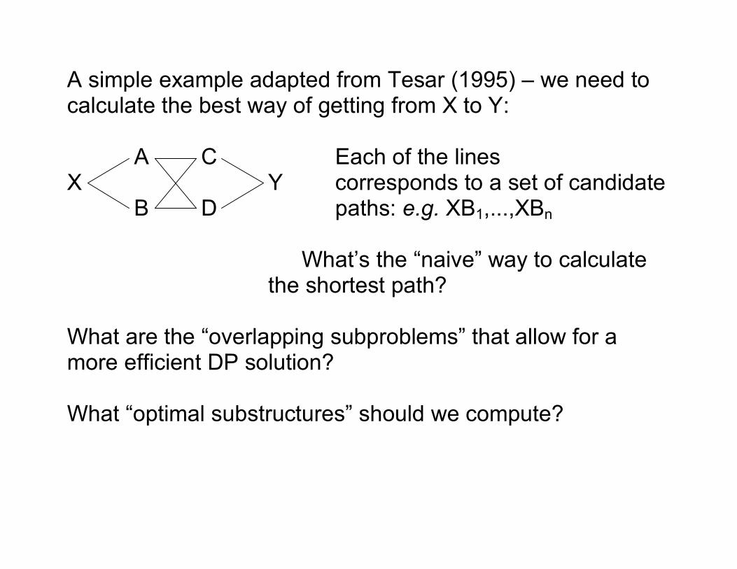
A simple example adapted from Tesar (1995) – we need to calculate the best way of getting from X to Y: A C Each of the lines X Y corresponds to a set of candidate B D paths: e.g. XB1,...,XBn

What’s the “naive” way to calculate the shortest path?

What are the “overlapping subproblems” that allow for a more efficient DP solution? What “optimal substructures” should we compute?

We can divide our problem into stages: stage 1 includes X, stage 2 includes A and B, and so on. At each stage we have a set of states: A and B are the states at stage 1. As we proceed through the stages, there will always be an optimal path to each of the current states (sometimes more than one) We do not need to recalculate the optimal path as we move through the stages: later decisions cannot affect earlier ones

From an introduction to dynamic programming:2

(3) If you study this procedure, you will find that the

calculations are done recursively. Stage 2 calculations are based on stage 1, stage 3 only on stage 2. Indeed, given you are at a state, all future decisions are made independent of how you got to the state. This is the principle of optimality and all of dynamic programming rests on this assumption.

2 http://mat.gsia.cmu.edu/classes/dynamic/dynamic.html

In Tesar’s OT syllable parser, what are the stages? What are the states?

The stages are defined by the segments of the input (L-R), plus “BOI” - beginning of input. The (non-vacuous) states are: (4) End in onset End in nucleus End in coda At each stage, we find the optimal way of ending up in one of these states, where optimal is defined in terms of the language’s constraint hierarchy.

The procedure is defined in terms of a table, with the columns representing the stages and the rows the states. We fill in the cells in a single column before moving on to the next. To fill in a cell, we: (5) a. Take the structure from a previous cell

b. Add the structure defined for the current stage (if it is

not already present - that is, if a. was in another column)

c. Apply an operation that brings the structure into the state defined for the cell

There are usually several paths that fit the description in (5): we choose the one that best satisfies the constraint hierarchy: the optimal one.

This case is more complex than the shortest path problem we looked at before:

(6) We can get to a state within one of the stages by going through another state in that same stage.

For example, when our current stage is defined by a C, ending in a nucleus can be achieved by going through the “end in onset” state (7) Two states in a single stage End in onset: o End in nucleus: o – n | |

C C

The most complex, and important, part of the algorithm involves the generation of the cell entries in a single column. This is where we get the finiteness result. We can see part of this finiteness result already at the BOI stage, the first column of the derivation (Tesar p. 111): Set [S,BOI] to no structure and no violation marks

Fill each other cell in column BOI with the best overparsing operation that currently applies Repeat until no cell entries change For each row X in BOI For each overparsing operation OP for X

If Harmony(OP(BOI)) > Harmony(X,BOI), set [X, BOI] to OP(BOI)

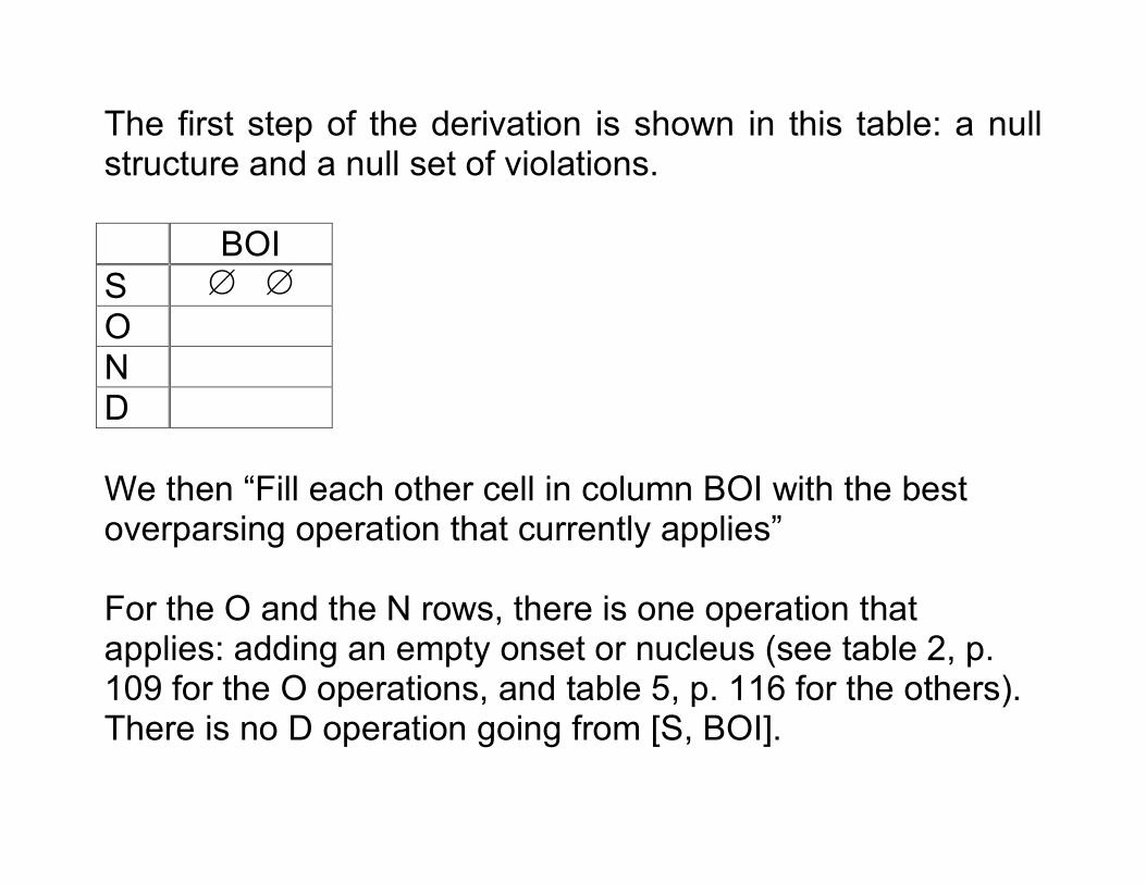
The first step of the derivation is shown in this table: a null structure and a null set of violations.

BOI

S ! !

O N D

We then “Fill each other cell in column BOI with the best overparsing operation that currently applies” For the O and the N rows, there is one operation that applies: adding an empty onset or nucleus (see table 2, p. 109 for the O operations, and table 5, p. 116 for the others). There is no D operation going from [S, BOI].

I’ve indicated empty structures with the corresponding lowercase letter.

BOI

S ! !

O .o. *FILL-ONS

N .n. *FILL-NUC

D

Next step(s):

Repeat until no cell entries change For each row X in BOI For each overparsing operation OP for X

If Harmony(OP(BOI)) > Harmony(X,BOI), set [X, BOI] to OP(BOI)

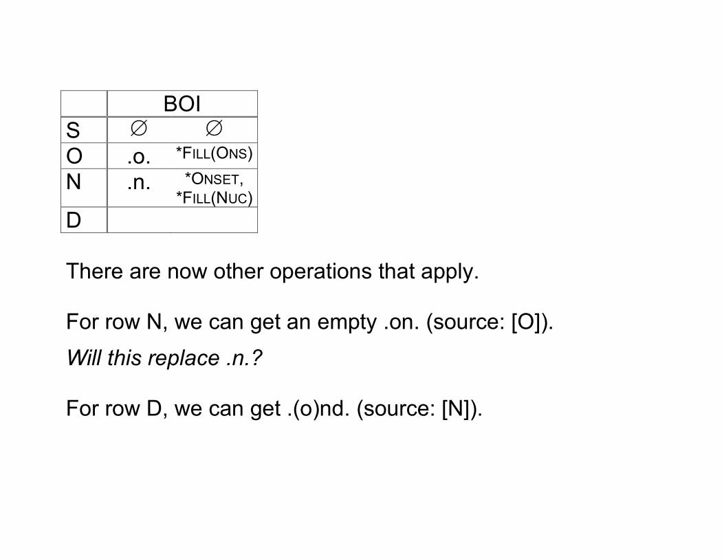
BOI

S ! !

O .o. *FILL(ONS)

N .n. *ONSET, *FILL(NUC)

D There are now other operations that apply. For row N, we can get an empty .on. (source: [O]).

Will this replace .n.? For row D, we can get .(o)nd. (source: [N]).

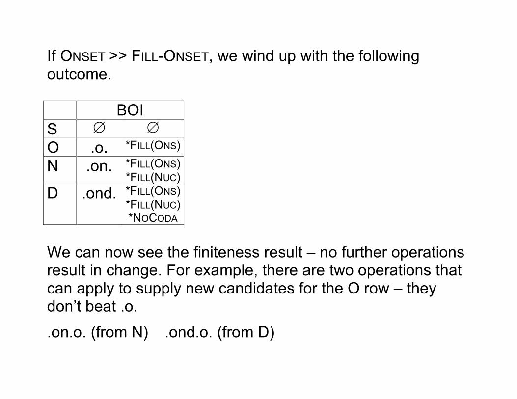
If ONSET >> FILL-ONSET, we wind up with the following outcome. BOI

S ! !

O .o. *FILL(ONS)

N .on. *FILL(ONS) *FILL(NUC)

D .ond. *FILL(ONS) *FILL(NUC) *NOCODA

We can now see the finiteness result – no further operations result in change. For example, there are two operations that can apply to supply new candidates for the O row – they don’t beat .o.

.on.o. (from N) .ond.o. (from D)

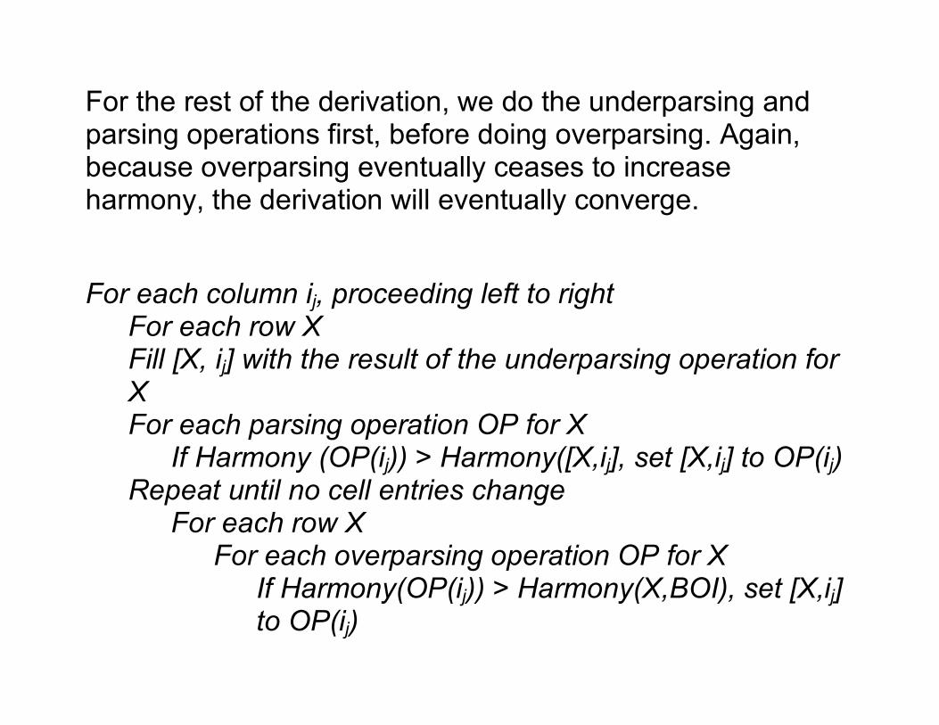
For the rest of the derivation, we do the underparsing and parsing operations first, before doing overparsing. Again, because overparsing eventually ceases to increase harmony, the derivation will eventually converge.

For each column ij, proceeding left to right For each row X

Fill [X, ij] with the result of the underparsing operation for X For each parsing operation OP for X If Harmony (OP(ij)) > Harmony([X,ij], set [X,ij] to OP(ij) Repeat until no cell entries change

For each row X For each overparsing operation OP for X

If Harmony(OP(ij)) > Harmony(X,BOI), set [X,ij] to OP(ij)

Two questions related to this course: (8) i. Is this Harmonic Serialism?

ii. What are the locality restrictions imposed by this parsing algorithm?

We can partly answer (8i.) simply by talking about the ways in which this parsing algorithm resembles, and diverges from, what we’ve been calling HS. It’s also instructive to consider a case in which HS diverges from parallel OT – for example, Berber syllabification.

McCarthy’s (2003) restatement of H-Nuc:

(9) *CONSONANTAL-NUCLEUS (*C-NUC)

Assign a violation mark to a nucleus for each degree of sonority separating it from [a]

For our example, we can simplify:

(10) *C-NUC violations

Vowel = 0, Sonorant C = 1, Fricative = 2, Stop = 3

(11) Step 1 /k!m/ *C-NUC

(K)!m 3! k(")m 2! ! k!(M) 1

(12) Step 2 /k!M/ *C-NUC

(K)!(M) 3! k(")(M) 2 ! k(!M)

(13) Step 3

/k(!M)/ *C-NUC

! (K)(!M) 3 (14) Wrong result in parallel OT

/k!m/ *C-NUC

(K)(!M) 3! (+1 = 4!)

! (k"m) 2

Because the operations add not only the structure, but also the violation marks, the algorithm imposes locality restriction on the constraints (p. 115): “What really matters here is that the constraint violations incurred by an operation can be determined solely on the basis of the operation itself. The information used by the constraints in the Basic Syllable Theory include the piece of structure added and the very end of the partial description being added on to (the last syllabic position generated). These restrictions on constraints are sufficient conditions for the kind of algorithm given in this paper. Ongoing work which cannot be discussed here investigates what actual restrictions on constraints are necessary.”

It strikes me that OCP-VOICE may be problematic in this respect; if we are parsing L-R, we don’t know if parsing a [voice] feature will add an OCP-Voice violation...

The Fibonacci numbers: (15) The first number of the sequence is 0, the second

number is 1, and each subsequent number is equal to the sum of the previous two numbers.

Dynamic Programming can facilitate the calculation of the value of the nth number in this sequence, Fn. If we use a “naive” method, we’ll wind up calculating previous members of the sequence more than once. Interestingly, the “Fibonacci” sequence was not first discovered by Leonardo of Pisa, or Fibonacci, but by the Sanskrit grammarians, in calculating the size of metrical “candidate sets”

Origins of the Fibonacci sequence3

The Fibonacci numbers first appeared, under the name m#tr#meru (mountain of cadence), in the work of the Sanskrit grammarian Pingala (Chandah-sh#stra, the Art of Prosody, 450 or 200 BC). Prosody was important in ancient Indian ritual because of an emphasis on the purity of utterance. The Indian mathematician Virahanka (6th century AD) showed how the Fibonacci sequence arose in the analysis of metres with long and short syllables. Subsequently, the Jain philosopher Hemachandra (c.1150) composed a well-known text on these. A commentary on Virahanka's work by Gop#la in the 12th century also revisits the problem in some detail.

3 http://en.wikipedia.org/wiki/Fibonacci_sequence

Sanskrit vowel sounds can be long (L) or short (S), and Virahanka's analysis, which came to be known as m#tr#-

v!tta, wishes to compute how many metres (m#tr#s) of a

given overall length can be composed of these syllables. If the long syllable is twice as long as the short, the solutions are: 1 mora: S (1 pattern) 2 morae: SS; L (2) 3 morae: SSS, SL; LS (3) 4 morae: SSSS, SSL, SLS; LSS, LL (5) 5 morae: SSSSS, SSSL, SSLS, SLSS, SLL; LSSS, LSL, LLS (8) 6 morae: SSSSSS, SSSSL, SSSLS, SSLSS, SLSSS, LSSSS, SSLL, SLSL, SLLS, LSSL, LSLS, LLSS, LLL (13)

7 morae: SSSSSSS, SSSSSL, SSSSLS, SSSLSS, SSLSSS, SLSSSS, LSSSSS, SSSLL, SSLSL, SLSSL, LSSSL, SSLLS, SLSLS, LSSLS, SLLSS, LSLSS, LLSSS, SLLL, LSLL, LLSL, LLLS (21) A pattern of length n can be formed by adding S to a pattern of length n!1, or L to a pattern of length n$2; and the prosodicists showed that the number of patterns of length n is the sum of the two previous numbers in the sequence.