dynamics of wess-zumino-witten and chern-simons...
TRANSCRIPT
UNIVERSIDAD DE SANTIAGO DE CHILE
DEPARTAMENTO DE FISICA, FACULTAD DE CIENCIA
Dynamics of Wess-Zumino-Witten
and Chern-Simons Theories
Olivera Miskovic
Thesis for obtaining the degree of
Doctor of Philosophy
Supervising Professors: Dr. Ricardo Troncoso
Dr. Jorge Zanelli
SANTIAGO – CHILE
JANUARY 2004
UNIVERSIDAD DE SANTIAGO DE CHILE
DEPARTAMENTO DE FISICA, FACULTAD DE CIENCIA
Dinamica de las Teorıas de
Wess-Zumino-Witten y Chern-Simons
Olivera Miskovic
Tesis para optar el grado de
Doctor en Ciencias con Mencion en Fısica
Directores de Tesis: Dr. Ricardo Troncoso
Dr. Jorge Zanelli
SANTIAGO – CHILE
ENERO 2004

INFORME DE APROBACION
TESIS DE DOCTORADO
Se informa al Comite del Programa de Doctorado en Ciencias con mencion
en Fısica que la Tesis presentada por el candidato
Olivera Miskovic
ha sido aprobada por la Comision Informante de Tesis como requisito para
la obtencion del grado de Doctor en Ciencias con mencion en Fısica.
Directores de Tesis:
Dr. Ricardo Troncoso
Dr. Jorge Zanelli
Comision Informante de Tesis:
Dr. Maximo Banados
Dr. Jorge Gamboa
Dr. Marc Henneaux
Dr. Mikhail Plyushchay
Dr. Lautaro Vergara (presidente)
Abstract
This thesis is devoted to the study of three problems on the Wess-Zumino-Witten
(WZW) and Chern-Simons (CS) supergravity theories in the Hamiltonian framework:
1. The two-dimensional super WZW model coupled to supergravity is constructed.
The canonical representation of Kac-Moody algebra is extended to the super Kac-Moody
and Virasoro algebras. Then, the canonical action is constructed, invariant under local
supersymmetry transformations. The metric tensor and Rarita-Schwinger fields emerge
as Lagrange multipliers of the components of the super energy-momentum tensor.
2. In dimensions D ≥ 5, CS theories are irregular systems, that is, they have con-
straints which are functionally dependent in some sectors of phase space. In these cases,
the standard Dirac procedure is not directly applicable and must be redefined, as it is
shown in the simplified case of finite number of degrees of freedom. Irregular systems
fall into two classes depending on their behavior in the vicinity of the constraint sur-
face. In one case, it is possible to regularize the system without ambiguities, while in the
other, regularization is not always possible and the Hamiltonian and Lagrangian descrip-
tions may be dynamically inequivalent. Irregularities have important consequences in the
linearized approximation of nonlinear theories.
3. The dynamics of CS supergravity theory in D = 5, based on the supersymmetric
extension of the AdS algebra, su(2, 2 |4), is analyzed. The dynamical fields are the viel-
bein, the spin connection, 8 gravitini, as well as SU(4) and U(1) gauge fields. A class
of backgrounds is found, providing a regular and generic effective theory. Some of these
backgrounds are shown to be BPS states. The charges for the simplest choice of asymp-
totic conditions are obtained, and they satisfy a supersymmetric extension of the classical
WZW4 algebra, associated to su(2, 2 |4).
i
Resumen
Esta tesis esta dedicada al estudio de tres problemas en de teorıas de supergravedad de
Wess-Zumino-Witten (WZW) y de Chern-Simons (CS), en el formalismo hamiltoniano:
1. Se construye un modelo de super WZW en dos dimensiones, acoplado a super-
gravedad. La representacion canonica del algebra de Kac-Moody es extendida a las
algebras de super Kac-Moody y super Virasoro. Luego, se construye la accion canonica,
invariante bajo transformaciones de supersimetrıa locales. El tensor metrico y el campo
de Rarita-Schwinger aparecen como multiplicadores de Lagrange de las componentes del
super tensor energıa-momentum.
2. En dimensiones D ≥ 5, las teorıas de CS constituyen sistemas irregulares, es decir,
contienen ligaduras que son funcionalmente dependientes en algunos sectores del espacio
de fase. En estos casos, el procedimiento de Dirac estandar no es aplicable directamente
y debe ser redefinido, como se muestra en el caso simplificado cuando el sistema tiene
un numero finito de grados de libertad. Los sistemas irregulares pueden pertenecer a dos
clases, dependiendo de su comportamiento en la vecindad de la superficie de ligadura. En
un caso, es posible regularizar el sistema sin ambiguedades, mientras que en el otro, la reg-
ularizacion no es siempre posible y las descripciones hamiltoniana y lagrangiana pueden no
ser dinamicamente equivalentes. Estas irregularidades tienen importantes consecuencias
en la aproximacion linealizada de teorıas no-lineales.
3. Se analiza la dinamica de la teorıa de supergravedad de CS en D = 5, basada en
la extension supersimetrica del algebra de AdS, su(2, 2 |4). Los campos dinamicos son el
vielbein, la coneccion de spin y 8 gravitini, ademas de campos de gauge para SU(4) y U(1).
Se identifica una clase de backgrounds que da lugar a una teorıa efectiva que es regular
y generica. Del mismo modo, se prueba que algunos de estos backgrounds son estados
BPS. Se obtienen las cargas para la eleccion mas simple de condiciones asintoticas. Estas
cargas satisfacen una extension supersimetrica del algebra clasica de WZW4, asociada a
su(2, 2 |4).
ii

Rezime
Ova teza je posveena prouqavanju tri problema u vezi sa Ves-Zumino-
Vitenovim (VZV) i Qern-Sajmonsovim (QS) teorijama supergravitacije u
okviru Hamiltonovog formalizma:
1. Konstruisan je dvodimenzioni super VZV-ov model kuplovan sa super-
gravitacijom. Kanonska reprezentacija Kac-Mudijeve algebre je proxirena
do supersimetriqne Kac-Mudijeve i Virazorove algebre, a zatim je konstru-
isano kanonsko dejstvo invarijantno pod transformacijama lokalne super-
simetrije. Metriqki tenzor i Rarita-Xvingerovo polje su se pojavili kao
Lagranevi mnoitelji uz komponente supertenzora energije-impulsa.
2. QS-ove teorije u dimenzijama D ≥ 5 su iregularni sistemi, xto znaqi
da sadre veze koje su funkcionalno zavisne u pojedinim oblastima faznog
prostora. U tim sluqajevima ne moe direktno da se primeni standardna
Dirakova procedura, nego mora da se redefinixe, xto je uraeno za naj-
jednostavnije sisteme sa konaqnim brojem stepeni slobode. Pokazano je da
postoje dve vrste iregularnih sistema, u zavisnosti od toga kako se ponaxaju
u blizini povrxi definisane vezama. U jednom sluqaju sistem moe da se
regularixe, dok u drugom sluqaju regularizacija nije uvek mogua, poxto
Hamiltonov i Lagranev formalizam mogu da dovedu do dinamiqki neekvi-
valentnih rezultata. Iregularnosti imaju znaqajne posledice u linearnoj
aproksimaciji nelinearnih teorija.
3. Analizirana je dinamika QS-ove teorije supergravitacije u D = 5,
bazirane na supersimetriqnoj ekstenziji anti-de Siterove algebre, su(2, 2|4).
Dinamiqka polja te teorije su pentada, spinska koneksija, 8 gravitina, kao i
gradijentna polja SU(4) i U(1). Naena je klasa pozadinskih polja takvih da
su efektivne teorije, definisane u njihovoj okolini, regularne i generiqke.
Takoe je pokazano da neka od tih pozadinskih polja predstavljaju tzv. BPS-
stanja. Izborom najjednostavnijih asimptotskih uslova su dobijeni oquvani
naboji, qija je algebra supersimetriqna ekstenzija klasiqne WZW4 algebre,
asocirane sa su(2, 2|4).
iii
Acknowledgment
There are many people who supported me from the moment I left my home in Belgrade, and
came to Chile to work on my Ph.D. Thesis. First of all, I thank to my parents and my sister,
without whose care, support and positive influence my trip and this work would have not been
possible. I will also be in eternal debt to Rodrigo Olea, who has been sharing with me his love,
his life and his knowledge in physics, and without whom everything would have been different.
The person who particularly fills me with the gratitude is my supervisor Jorge Zanelli, whose
love for physics and his profound understanding of it have been irresestibly inspiring, and whose
deep humanity is overwhelming. Infinite thanks to Ricardo Troncoso, my second supervisor and
friend, for his help, support and cheering up in dark moments. I would like to thank to all
physicists and staff of CECS, with the director Claudio Teitelboim, who accepted me from the
very beginning as a member of their “second family”.
For enlightening and useful discussions, as well as friendly criticism, thanks to Alexis Amezaga,
Rodrigo Aros, Eloy Ayon-Beato, Maximo Banados, Arundhati Dasgupta, Andres Gomberoff,
Mokhtar Hassaıne, Marc Henneaux, Georgios Kofinas, Cristian Martınez, Rodrigo Olea, Mikhail
Plyushchay, Joel Saavedra, Claudio Teitelboim and Tatjana Vukasinac. I am particularly thank-
full to Milutin Blagojevic, Ivana Miskovic and Branislav Sazdovic, who were regularly replying
my numerous questions by e-mail, and to Milovan Vasilic, for his helpful criticism. Many thanks
to all physicists and staff of Institute of Physics in Belgrade, Vinca Institute and the Department
of Physics USACH.
I will be forever obliged to my friends Aleksandra Cuk, Snezana Djurdjic, Dafni Fernanda
Zenedin Marchioro, Milan Lalic, Aleksandra Lazovic, Ricardo Navarro, Ljubomir Nikolic, Ivan
Sajic, Jelena Tosic and Tatjana Vukasinac, for their friendship and moral support.
This work is partially funded by Chilean grants JZ 1999, MECESUP USA 9930, FONDE-
CYT 2010017 and Millenium Project. I also want to thank to the Abdus Salam ICTP, Max
Planck-Albert Einstein Institut and Universite Libre de Bruxelles for their hospitality during
the completition the parts of this work, as well as to Sonja and Vlado Miskovic for their finan-
cial help. The generous support of Empresas CMPC to CECS is also acknowledged. CECS is
a Millenium Science Institute and is funded in part by grants from Fundacion Andes and the
Tinker Foundation.
iv
Contents
1 Introduction 1
2 Wess-Zumino-Witten model 7
2.1 The action . . . . . . . . . . . . . . . . . . . . . . . . . . . . . . . . . . . . 7
2.2 Kac-Moody algebra . . . . . . . . . . . . . . . . . . . . . . . . . . . . . . . 9
2.3 Virasoro algebra . . . . . . . . . . . . . . . . . . . . . . . . . . . . . . . . . 14
2.4 Gauged WZW model . . . . . . . . . . . . . . . . . . . . . . . . . . . . . . 16
2.5 Supersymmetric WZW model . . . . . . . . . . . . . . . . . . . . . . . . . 17
3 Supersymmetric WZW model coupled to supergravity 22
3.1 Super Virasoro generators . . . . . . . . . . . . . . . . . . . . . . . . . . . 22
3.2 Effective Lagrangian and gauge transformations . . . . . . . . . . . . . . . 28
3.3 Lagrangian formulation . . . . . . . . . . . . . . . . . . . . . . . . . . . . . 30
3.4 Conclusions . . . . . . . . . . . . . . . . . . . . . . . . . . . . . . . . . . . 33
4 Irregular constrained systems 34
4.1 Regularity conditions . . . . . . . . . . . . . . . . . . . . . . . . . . . . . . 34
4.2 Basic types of irregular constraints . . . . . . . . . . . . . . . . . . . . . . 36
4.3 Classification of constraint surfaces . . . . . . . . . . . . . . . . . . . . . . 37
4.4 Treatment of systems with multilinear constraints . . . . . . . . . . . . . . 39
4.5 Systems with nonlinear constraints . . . . . . . . . . . . . . . . . . . . . . 42
4.6 Some implications of the irregularity . . . . . . . . . . . . . . . . . . . . . 45
4.7 Summary . . . . . . . . . . . . . . . . . . . . . . . . . . . . . . . . . . . . 48
v
5 Higher-dimensional Chern-Simons theories as irregular systems 50
5.1 Chern-Simons action . . . . . . . . . . . . . . . . . . . . . . . . . . . . . . 50
5.2 Hamiltonian analysis of Chern-Simons theories . . . . . . . . . . . . . . . . 52
5.3 Regularity conditions . . . . . . . . . . . . . . . . . . . . . . . . . . . . . . 56
5.4 Conclusions: the phase space of CS theories . . . . . . . . . . . . . . . . . 60
6 AdS -Chern-Simons supergravity 62
6.1 D = 5 supergravity . . . . . . . . . . . . . . . . . . . . . . . . . . . . . . . 63
6.2 Conserved charges . . . . . . . . . . . . . . . . . . . . . . . . . . . . . . . 66
6.3 Killing spinors and BPS states . . . . . . . . . . . . . . . . . . . . . . . . . 74
6.4 Conclusions . . . . . . . . . . . . . . . . . . . . . . . . . . . . . . . . . . . 78
7 List of main results and open problems 81
A Hamiltonian formalism 83
B Superspace notation in D = 2 92
C Components of the vielbein and metric in the light-cone basis 94
D Symplectic form in Chern-Simons theories 96
E Anti-de Sitter group, AdSD 99
F Supersymmetric extension of AdS 5, SU(2, 2 |N ) 101
G Supergroup conventions 106
H Killing spinors for the AdS 5 space-time 109
vi
Chapter 1
Introduction
Wess-Zumino-Witten (WZW) and Chern-Simons (CS) field theories have been intensively
studied in connection with several applications in physics and mathematics.
The two-dimensional WZW theory1 [1, 2, 3], described by a non-linear sigma model
with non-local interaction, was originally studied by Witten [3] as a theory equivalent
to non-interacting massless fermions, thus providing non-Abelian bosonization rules for
interacting fermionic theories. The WZW action is also known as the necessary counter-
term for cancelation of quantum anomalies (the breaking down of a classical symmetry at
the quantum level) [4]–[8]. This theory is exactly solvable and quantizable, and its action
has two independent (“left” and “right”) chiral symmetries, whose infinite-dimensional
algebras are two copies of the affine, Kac-Moody (KM), algebra. The WZW theory is also
conformally invariant, where the symmetry is described by the Virasoro algebra. Because
of this, the WZW model is relevant in string theory, as well.
Three-dimensional CS theories have a topological origin, since they can be defined as
CS forms integrated over the boundary of a compact four-dimensional manifold. These
theories have no local degrees of freedom and they are also exactly solvable and quantizable
[9]. As topological field theories, they can be used in the classification of three-dimensional
manifolds [10]. The quantum CS theories are known to describe the quantum Hall effect
[11]. CS theories can also be defined on three-dimensional manifolds with a boundary. In
that case, their transformations under the “large” gauge transformations are non-trivial
1This is also called Wess-Zumino-Novikov-Witten (WZNW) theory.
1
and given by a closed 3-form, that has been used in the context of quantum anomalies.
The fact that both WZW and CS theories are related to the quantum anomalies is not
accidental. Their relation reflects a profound connection between them. For example, the
gauge transformations of the CS action give a non-trivial contribution to the gauged WZW
model describing the most general form of a two-dimensional chiral anomaly [12]–[15]. Any
CS theory defined on a three-manifold with a boundary, induces a two-dimensional WZW
model as a topological field theory [10, 16, 17].
In general, the dynamics at the boundary is determined by the asymptotic behavior
of the fields. This is essential for a suitable definition of the global charges of the theory
[18]–[20].
The most interesting aspect of these two classes of theories, which will be further
investigated, is their deep connection with lower-dimensional gravity theories. For exam-
ple, two-dimensional induced gravity can be obtained as a gauge extension of the WZW
model [21, 22, 23], while the Liouville theory, describing the asymptotic dynamics of three-
dimensional Einstein-Hilbert gravity with negative cosmological constant, is equivalent to
the two-dimensional induced gravity in the conformal gauge [24, 25].
On the other hand, three-dimensional gravity, described by the Einstein-Hilbert ac-
tion, which is linear in the curvature of space-time, can be formulated as a CS gauge
theory invariant under de Sitter (dS ), anti-de Sitter (AdS ) or Poincare groups [26, 27, 28].
Asymptotically locally AdS gravity, for example, has an infinite-dimensional algebra of
asymptotic symmetries described by the Virasoro algebra, whose realization in terms of
conserved charged requires a non-trivial classical central charge [29].
The need to look for alternative gravity theories arises from the fact that General
Relativity, which gives a successful classical description of gravitational phenomena in
four dimensions, does not admit a standard quantum description yet, while the other
three fundamental forces are consistently unified and described by quantum theories of
the Yang-Mills (YM) type. In this approach, the main obstruction for existence of a
quantum theory of gravity is its nonrenormalizability, i.e., the impossibility of removing
all divergences which appear in the high-energy sector of the theory, due to the dimension
of gravitational constant. While the renormalizability of YM theories is a consequence
of their invariance under local gauge transformations, since the gauge principle provides
2
a dimensionless coupling constant, the Einstein-Hilbert theory is invariant under general
coordinate transformations x → x′ = x′(x) (diffeomorphisms). This symmetry, however,
does not guarantee the consistency of the quantum theory, because this symmetry does
not have a fiber-bundle structure as in YM theories (which is sufficient, but not necessary
condition for a theory to be renormalizable).
Supersymmetry is naturally introduced, since supersymmetric theories can lead to a
non-trivial unification of space-time and internal symmetries within a relativistic quantum
field theory (see, e.g., [30]–[32]). In these theories, both bosons and fermions belong to the
same representation of the supergroup. The gravitational interaction emerges naturally
from local supersymmetry, since the anticommutator of two supersymmetry generators
(supercharges) gives a generator of local translations. In that way, supergravity theories
are obtained as supersymmetric extensions of the purely gravitional part.
Furthermore, supersymmetric extensions of chiral and conformal symmetries define
supersymmetric WZW models, characterized by super KM and super Virasoro algebras
[33]. In three dimensions, these superalgebras are obtained as the algebra of the classical
charges for AdS supergravity models, with adequate asymptotic conditions [34, 35].
The existence of supersymmetry makes possible to construct non-negative quantities
quadratic in the supercharges, which gives rise to the inequalities known as Bogomol’nyi
bounds [36]. These bounds guarantee the stability of the ground state (vacuum) in su-
pergravity theories, so that it remains a state of minimal energy after perturbations.
The Bogomol’nyi bound ensures the positivity of energy in the standard supergravities
[37, 38, 39], even in presence of other conserved quantities [40].
Higher-dimensional theories can be physically meaningful if one supposes that only
four dimensions of space-time are observable, while others are “too small” to be visible
at currently reachable energies. In that sense, a four-dimensional theory would be an
effective theory. This can be realized by the procedure known as dimensional reduction,
where one assumes that the radius of extra dimensions is compactified beyond sight (see,
e.g., [41, 42]).
It is interesting, thus, to consider higher-dimensional CS theories, which are defined
in all odd dimensions, and have Lagrangians represented by CS forms [43]–[47]. CS
gravity and supergravity theories are based on the anti-de Sitter [AdS, or SO(D − 1, 2)],
3
de Sitter [dS, or SO(D, 1)], and Poincare [ISO(D − 1, 1)] gauge groups, as well as their
supersymmetric extensions. They are by construction invariant under diffeomorphisms
and provide a non-standard, consistent description of gravity as a gauge theory [48]–[52].
They are genuine gauge theories which are extensions of the Einstein-Hilbert action. Their
actions are polynomials in the curvature R and they can also depend explicitly on the
torsion T . Furthermore, they possess propagating degrees of freedom [54, 55], and have a
very rich phase space structure. In CS supergravities, unlike in the standard supergravity
theories, the supersymmetry algebra closes off shell, without addition of the auxiliary
fields [56].
On the other hand, WZW and super WZW theories could be generalized to higher di-
mensions as field theories whose symmetries are described by (supersymmetric) extensions
of KM and Virasoro algebras. They are not studied as much as in the two-dimensional
case. For example, the WZW action is known in four dimensions, with the local sym-
metry described by a four-dimensional extension of the KM algebra, or WZW4 algebra
[46, 47, 57]. The relation between this four-dimensional WZW theory and a CS theory
in five dimensions is established only at the level of algebras [55], while the actions has
not been obtained explicitly. In general, the action of the four-dimensional super WZW
model remains unknown.
Higher-dimensional CS theories have complex configurational space. In five-dimensi-
onal CS supergravity, for example, it was observed that the linearized action around an
AdS background seems to have one more degree of freedom than the full nonlinear system
[58]. This paradoxical behavior arises from the violation of the regularity conditions
among the symmetry generators of the theory, or their functional dependence, in the
region of phase space defined by the selected background. Therefore, CS theories in
D ≥ 5 dimensions are irregular systems, where Dirac’s standard procedure of finding
local symmetries and physical degrees of freedom [59] fails.2 The problem of the regularity
does not appear in lower-dimensional WZW or CS theories, but can occur in any physical
system, independently of the dimension of space-time.
Constraints satisfying regularity conditions are sometimes referred to as effective con-
2A well-known example of an irregular system is a relativistic massless particle (pµpµ = 0), which is
irregular at the origin of momentum space (pµ = 0).
4
straints [60]. The issue of regularity (effectiveness) and its relevance for the equivalence
between the Lagrangian and Hamiltonian formalisms has also been discussed in several
references [61, 62, 63].
There are many different areas where the WZW and CS theories find their applications
but, from the point of view of this thesis, the main motivation to study these theories is:
(i) CS theories are alternative gravity and supergravity theories in odd dimensions, (ii)
every AdS -CS theory induces a conformal field theory at the boundary, a WZW model,
and (iii) WZW models should correspond to (super)gravity theories in even dimensions.
Therefore, three problems related to CS theories and to the topics (i)-(iii) are pre-
sented in this thesis, where each one can be analyzed independently.
• The first problem is the construction of the super WZW model coupled to super-
gravity, from the chosen canonical representation of the super Virasoro algebra. The
model is obtained explicitly in two dimensions [64], what may provide some insight
for finding the unknown four-dimensional super WZW theory.
• The second question arises from the need of dealing with irregular CS systems,
and of generalizing the Dirac procedure. The problem is analyzed for classical
mechanical systems with finite number of degrees of freedom [65, 66], and discussed
in CS theories as well [66].
• The third part presents a work currently in progress, based on the study of the dy-
namical structure of five-dimensional AdS -CS supergravity, both in the bulk and at
the boundary. The physical degrees of freedom and local symmetries of these theo-
ries depend on the symplectic form (defining the kinetic term). Since the symplectic
form is a function of phase space coordinates whose rank can vary throughout the
phase space, CS theories can be either regular, or irregular [66]. Moreover, they
can be generic, with a minimal number of local symmetries [55], or degenerate if
the symplectic form has a lower rank and additional symmetries emerge [67, 68].
In the asymptotic sector, the charge algebra of the AdS -CS supergravity is the
supersymmetric extension of the WZW4 algebra with a central charge [69].
The thesis is organized as follows.
5
In Chapter 2, the two-dimensional WZW model is reviewed. Two independent KM
algebras are obtained as canonical symmetries of the WZW action. The conformal sym-
metry in this model is not independent, since the Virasoro generators can be expressed as
bilinears of the KM generators. The super WZW model is also discussed, using superspace
formalism.
In Chapter 3, two-dimensional WZW supergravity is constructed using the Hamilto-
nian method. The canonical (first order) action is defined from the phase space represen-
tation of the super Virasoro algebra, and the Lagrange multipliers corresponding to the
super Virasoro generators appear as the components of the metric field and gravitini.
In Chapter 4, Dirac’s procedure is extended to irregular classical mechanical systems
with finite number of degrees of freedom. These systems are classified, and regularized
when possible, by introducing dynamically equivalent regular Lagrangians. It is shown
that a system cannot evolve in time from a regular phase space configuration into an
irregular one, since regular and irregular configurations always belong to sectors of phase
space that do not intersect.
In Chapter 5, the dynamical structure of the higher-dimensional CS theories is studied,
where the symmetries are analyzed using canonical methods. Criteria which determine
whether the regularity and genericity conditions are satisfied around the chosen back-
ground, are presented.
In Chapter 6, five-dimensional AdS -CS supergravity theory, based on SU(2, 2 |N )
group, is studied, as the simplest example of CS supergravity theories with propagating
degrees of freedom. In the particular case of N = 4, a class of generic and regular
backgrounds is found, such that all charges can be defined at the boundary. Among
them, there are configurations which are BPS states. The classical charge algebra is
obtained as the supersymmetric extension of the WZW4 algebra with a central extension.
The main results of the Thesis were published in Refs. [64, 65, 66], and the manuscript
[69] is in preparation.
6
Chapter 2
Wess-Zumino-Witten model
Wess-Zumino-Witten (WZW) models are conformal field theories in which an affine, or
Kac-Moody (KM) algebra gives the spectrum of the theory. The two-dimensional WZW
model studied here is a system whose kinetic term is given by the nonlinear sigma model
and the potential is the Wess-Zumino term [1, 2]. This model was originally studied
by Witten in the context of two-dimensional bosonization, where it provides non-Abelian
bosonization rules describing non-interacting massless fermions [3]. The WZW action was
also used as a term cancelling quantum anomalies [4]–[8]. It is a chirally and conformally
invariant theory, and exactly solvable.
The purpose of this chapter is to present the WZW model and its global and local
symmetries in a systematic way, as well as to introduce the notation. In the next chapter,
a general idea of finding an action, starting only from the algebra of its local symmetries,
will be presented in two dimensions and for N = 1 superconformal group. It will be shown
that, in that way, the super Virasoso algebra leads to the super WZW model coupled to
supergravity.
2.1 The action
The two-dimensional WZW model has a fundamental field g belonging to a non-Abelian
semi-simple compact Lie group G and the dynamics given by the action
7
IWZW [g] = I0 [g] + Γ [g] = −a∫M
〈∗VV〉 − k
3
∫B
⟨V3⟩ (
V ≡ g−1dg), (2.1)
where I0 [g] is the action of the non-linear σ-model with a positive dimensionless coupling
constant a, while Γ [g] is the topological Wess-Zumino term defined over a three-manifold
B whose boundary is the two-dimensional space-time, ∂B =M, and k is a dimensionless
constant. Here V is a Lie-algebra-valued one-form, ∗V is its Hodge-dual and 〈· · · 〉 stands
for a trace. The exterior product ∧ between the forms is understood.
The Wess-Zumino term has a non-local expression, involving integration over the three-
manifold B, but it depends only on its boundary M modulo a constant. Independence
from the choice of B follows from the identity
1
12π
∫B
⟨V3⟩− 1
12π
∫B′
⟨V3⟩
= −2πn , (n ∈ Z) , (2.2)
with M = ∂B = ∂B′, which is a consequence of the index theorem. The set B ∪ B′ is
a closed oriented manifold, topologically equivalent to a three-sphere S3, provided the
boundaries of B and B′ have opposite orientations. Thus, the term 2πn in (2.2) arises
because of the topologically distinct possibilities to have the mapping g(x) : S3 → G, clas-
sified by π3 (G) ' Z (for G compact semi-simple), with the corresponding winding number
n. Therefore, all dynamics happens on the two-dimensional space-time M, provided the
constant k is proportional to an integer,
k =n
8π. (2.3)
Then, the quantum amplitude∫
[dA] eiIWZW[A] is independent of the choice of B, provided
the constant k is quantized as in (2.3).
Field equations. The local coordinates on M with the signature (−,+) are in-
troduced as xµ (µ = 0, 1). Then the differential forms can be expressed in the basis of
1-forms onM as V = g−1∂µg dxµ and ∗V = ε ν
µ g−1∂νg dxµ (with ε01 = 1). Under a small
variation of the gauge field, g → g + δg, the WZW action changes as
δIWZW [g] = −a∫d2x
⟨g−1δg ∂µ
(g−1∂µg
)⟩+ k
∫d2x εµν
⟨g−1δg ∂µ
(g−1∂νg
)⟩. (2.4)
8
In the light-cone coordinates x± = 1√2(x0 ± x1), it gives the following field equations:1
(a+ k) ∂−(g−1∂+g
)+ (a− k) ∂+
(g−1∂−g
)= 0 . (2.5)
Therefore, taking into account that a must be positive in order to have the right sign
in the kinetic term of (2.1), while the sign of k = n8π
depends on n ∈ Z, there are two
possible choices of a which give a theory with chiral symmetry. For a = −k and n < 0,
the equation of motion is ∂+ (g−1∂−g) = 0, with the general solution
g(x+, x−) = g+
(x+)g−(x−), (2.6)
where g+ and g− are elements of G. For a = k and n > 0, (2.5) becomes ∂− (g−1∂+g) = 0
and the general solution is factorized as g− (x−) g+ (x+). Equation (2.6) is invariant under
the left chiral transformations g+ (x+)→ Ω+ (x+) g+ (x+) and right chiral transformations
g− (x−)→ g− (x−)Ω−1− (x−), or
g(x+, x−)→ Ω+
(x+)g(x+, x−)Ω−1
−(x−), (Ω+,Ω−) ∈ G⊗G . (2.7)
This symmetry is related to two independent Kac-Moody algebras, as will be seen using
canonical methods.
2.2 Kac-Moody algebra
The symmetries of the WZW action (2.1) with a = −k > 0 can be found using the
Hamiltonian formalism [3, 70]. A summary of the formalism is given in Appendix A.
Let the local coordinates qi parametrize the group manifold, g = g(q), where the
number of coordinates is equal to the dimension of G, and the generators of the group
satisfy the Lie algebra [Ga,Gb] = f cab Gc. Then the Lie-algebra-valued 1-form V can be
expanded as
V = g−1dg = dqiEai Ga , (2.8)
1In the light-cone coordinates, the antisymmetric tensor becomes ε+− = −ε−+ = 1, and the metric
has non-zero components η+− = η−+ = −1.
9
where Eai is a vielbein on the group manifold. The Killing metric in the adjoint repre-
sentation of the Lie algebra is gab = 〈GaGb〉 = f cadf
dbc , and in the coordinate basis the
metric is
γij (q) = Eai (q)Eb
j (q) gab . (2.9)
On the basis of Poincare’s lemma, the equation d 〈V〉3 = 0 can be locally written as
exterior derivative of a two-form,
〈V〉3 = −6 dρ , (2.10)
where ρ ≡ 12ρij dq
idqj. Rewriting this in components, the following identities are obtained:
1
2fabc E
ai E
bjE
ck = ∂iρjk + ∂jρki + ∂kρij . (2.11)
Then the local expression for the action (2.1) in the light-cone coordinates becomes:
IWZW [g (q)] = −2k
∫d2x [γij (q) + 2ρij (q)] ∂−qi∂+q
j . (2.12)
Taking τ = x0 as canonical time, one finds that (2.12) has no first class constraints,
therefore has no local symmetries. But it is expected to find that this action possesses
two types of chiral symmetry which, unlike standard local symmetries, depend only on
one coordinate. The canonical approach to the chiral symmetries requires to take one
of the light-cone coordinates as the time variable. In order to find the complete chiral
invariance of (2.12), both possibilities τ = x− and τ = x+ should be analyzed.
a) Local symmetries
The space-time coordinates are chosen as (τ, σ) = (x−, x+). Then, the momenta pi = δIδqi
canonically conjugated to coordinates qi are not independent and define the constraints
K−i ≡ pi + 2k (γij + 2ρij) ∂σqj ≈ 0 , (2.13)
where the additional subindex “−” in K−i refers to the choice of τ , while ≈ denotes
the weak equality, since the derivatives of K−i do not vanish on the constraint surface
K−i = 0. An equivalent set of constraints (defining the same constraint surface) is
K−a = −EiaK−i ≈ 0 , (2.14)
10
where Eia is the inverse vielbein
(Ei
aEbi = δb
a and Eai E
ja = δj
i
). Then, the Hamiltonian
H =
∫dσ uaK−a (2.15)
depends on the arbitrary multipliers ua (τ, σ) and generates the time evolution of any
phase space variable F (q, p) by Poisson brackets (PB) as
dF
dτ= F,H . (2.16)
The constraints K−a ≈ 0 are preserved in time if ∂σu = 0, thus they do not yield new
constraints, and u = u (τ). The PB of constraints give rise to the affine, or KM, algebra
K−a (x) , K−b (x′) = f cabK−c (x) δ (σ − σ′)− 4kgab∂σδ (σ − σ′) , (2.17)
with the central extension −4k. Here x = (τ, σ) and the PBs are taken at the same τ .
The presence of the Schwinger term proportional to ∂σδ in (2.17) indicates that not all
constraints are first class, however, it is not clear how to identify first and second class
constraints. Assuming that the space is compact and all variables on M are periodic
functions, with period L, F (τ, σ + L) = F (τ, σ), they can be Fourier-expanded as
F (τ, σ) =1
L
∑n∈Z
Fn (τ) e−2πiL
nσ ←→ Fn (τ) =
L∫0
dσ F (τ, σ) e2πiL
nσ . (2.18)
Then, the KM algebra becomes
K−an, K−bm = f cab K−c(n+m) − 8πi kn gabδn+m,0 . (2.19)
The result does not depend on the period L, and now it is straightforward to separate
first and second class constraints. From
K−a0, K−bn = f cabK−cn ≈ 0 , (2.20)
it can be seen that the zero modes Ka0 are first class constrains and that they close the
PB subalgebra which is isomorphic to the algebra of G, while the non-zero modes Kan
(n 6= 0) are second class constraints,
K−an, K−b(−n)
≈ −8πi kn gab 6= 0 , (n 6= 0) . (2.21)
11
Therefore, the generator of gauge transformations, containing all first class constraints,
has the form
G− [λ] ≡ λa−K−a0 , (2.22)
with a local parameter λa− (τ). The dynamical field qi changes under infinitesimal gauge
transformations as
δ−qi =qi, G [λ]
= −λa
−Eia , (2.23)
which, with the help of the expansion g−1δ−g = δ−qiEai Ga, leads to the transformation
law g−1δ−g = −λ−, or
δ−g = −gλ− . (2.24)
The transformations (2.24) are the infinitesimal form of the right chiral gauge transfor-
mations
g → g Ω−1−(x−), (2.25)
with a group element defined as Ω− ≡ eλ− ≈ 1 + λ−.
Alternatively, choosing the space-time coordinates as (τ, σ) = (x+,−x−), where the
minus sign is adopted to preserve the orientation between coordinate axes, and with the
help of the identity
−gVg−1 = gdg−1 ≡ dqiEai Ga , (2.26)
the constraints take the form
K+a ≡ −Eia
[pi + 2k (γij − 2ρij) ∂σq
j]≈ 0 . (2.27)
They form an independent KM algebra,
K+a (x) , K+b (x′) = f cabK+c (x) δ (σ − σ′) + 4k gab∂σδ (σ − σ′) , (2.28)
with the central extension +4k, which has the opposite sign to that in (2.17). The mode
expansion gives the algebra (2.19) with k → −k and the corresponding first class gauge
12
generator G+ [λ] ≡ λa+K+a0 leads to right chiral transformations δ+g = λ+g, which are
the infinitesimal form of
g → Ω+
(x+)g , (2.29)
where Ω+ ≡ eλ+ ≈ 1 + λ+. The constraints K+a commute with K−b. Both results
(2.25) and (2.29) are independent gauge symmetries of the action. This means that the
action (2.12) is invariant under the chiral transformations (2.7) generated by K+a0 acting
from the right, and K−a0 acting from the left. The modes K±an, n 6= 0, are not the
generators of local symmetries (they are second class constraints), and they lead to the
central extensions ±4k in the corresponding KM algebras.
b) Global symmetries
Choosing the space-time coordinates as τ = x− and σ = x+, the infinitesimal chiral
transformations (2.7) of g ∈ G take a form
δ±g = λ+ (σ) g − gλ− (τ) , (2.30)
with the Lie-algebra-valued parameters λ± = λa±Ga or, in terms of the local fields qi, the
transformations become
δ±qi = −λa+ (σ) Ei
a − λa− (τ)Ei
a . (2.31)
Therefore, right chiral transformations, given by the time-dependent parameter λ− (τ),
lead to local symmetries of the WZW action. It is already shown that these symmetries
are generated by the first class constraints K−a0 ≈ 0.
On the other hand, left chiral transformations correspond to global symmetries of the
action, since they are given by infinite number of time-independent parameters λ+ (σ).
Conserved charges corresponding to these global symmetries are obtained from Noether
currents,
Ja+ ≡ 4k
(g∂+g
−1)a
= 4k Eai ∂σq
i , (2.32)
and they do not vanish on the constraint surface K−a = 0.
13
In order to find the current algebra, it is convenient to introduce a Dirac bracket (DB)
as
M,N∗ ≡ M,N −∑
m,n 6=0
M,K−an∆abnm K−bm, N , (2.33)
where ∆abnm ≡ 1
8πi kngabδn+m,0 (n,m 6= 0) is the inverse of the PB matrix of second class
constraints K−an (n 6= 0), given by Eq. (2.21). Then it can be shown that the currents
Ja+ satisfy the KM algebra with the central charge 4k,
J+a (x) , J+b (x′)∗ = f cab J+c (x) δ (σ − σ′) + 4k gab∂σδ (σ − σ′) . (2.34)
Similarly, choosing τ = x+ as canonical time, there are Noether currents J− =
4k g−1∂−g, corresponding to the right chiral symmetries as global symmetries of the WZW
model. The currents Ja− satisfy a KM current algebra with the central charge −4k.
2.3 Virasoro algebra
WZW theory is also invariant under conformal transformations, or diffeomorphisms xµ →x′µ(x) which change the line element by a scale factor at each point of space-time,
ds′2 = g′µν (x′) dx′µdx′ν = Λ (x) gµν (x) dxµdxν = Λ (x) ds2 . (2.35)
Conformal transformations have the form of chiral and antichiral mappings x+ → f+(x+)
and x− → f−(x−), and their generators are the light-cone components of the energy-
momentum tensor T++(x+) and T−−(x−), which is traceless (T µµ = 2T+− = 0). They
satisfy two independent Virasoro algebras,
[T (x), T (y)] = − [T (x) + T (y)] δ′(σx − σy)−c
12δ′′′(σx − σy) , (2.36)
without central charge (c = 0) in a classical theory, or with central charges c = c0 and
c = −c0 (for T++ and T−− respectively) in the quantum case. (The normalization of c
is adopted from string theory.) The appearance of the Schwinger term in the quantum
Virasoro algebra is called a quantum anomaly, but it can appear in a classical theory as
14
well [29]. The physical meaning of c 6= 0 in a classical theory is the breaking of confor-
mal symmetry by the introduction of a macroscopic scale into the system (by boundary
conditions, for example).
The Fourier modes of the Virasoro generators, Ln (n ∈ Z), in a compact space with
period L, are given by
Ln =L
2πi
L∫0
dσ T (σ) e2πiL
nσ, (2.37)
where L†n = L−n for unitary representations. They obey the well-known commutation
rules
[Ln, Lm] = (n−m)Ln+m +c
122πi n3δn+m,0 . (2.38)
This algebra contains a finite subalgebra, generated by L−1, L0, L1, associated to global
conformal invariance.
Conformal symmetry does not arise in the Hamiltonian analysis because it is not an
independent symmetry. Virasoro generators can be expressed in terms of KM currents as
[90, 91]
T−− =1
4kgabJ−aJ−b ,
T++ = − 1
4kgabJ+aJ+b , (2.39)
and they represent the light-cone components of the energy-momentum tensor. Conformal
invariance leads to T−+ = 0. In terms of the Fourier modes, the relations (2.39) become
L±n = ∓ 1
8πik
∑m∈Z
gabJ±amJ±b(n−m) . (2.40)
The observation that the energy-momentum tensor is a bilinear in the currents, is
used to construct them using the procedure of Sugawara [71, 72]. More precisely, for a
given KM algebra, there is always a Virasoro algebra, such that they form a semi-direct
product
[Ln, Jam] = 2mJa(n+m) , [Ln, K] = 0 , (2.41)
where K is the central extension of the KM algebra. More about Virasoro and KM
algebras in the conformal filed theory can be found in Refs. [73]–[76].
15
2.4 Gauged WZW model
The two-dimensional WZW model is closely related to a three-dimensional Chern-Simons
(CS) theory whose dynamical field is a Lie-algebra-valued 1-form, A = AaGa. Definition
of the CS Lagrangian comes from the Chern character,
P (A) =⟨F2⟩≡ gabF
aF b, (2.42)
where F = dA + A2 is the field-strength 2-form associated with the gauge field A. Since
the Chern character is a closed form (dP = 0), on the basis of algebraic Poincare’s lemma2,
it can be locally written as the exterior derivative of a 3-form, called the CS form, which
defines the CS Lagrangian as dLCS (A) = kP (A). Then the CS action is given by
ICS [A] =
∫B
LCS (A) = k
∫B
⟨AF− 1
3A3
⟩, (2.43)
where B is a three-dimensional manifold (not necessarily without a boundary).
Under finite gauge transformations
Ag = g (A + d) g−1 = g (A−V) g−1 , (g ∈ G) , (2.44)
the field-strength transforms homogeneously (Fg = gFg−1), the Chern character is invari-
ant and the CS Lagrangian changes as LgCS = LCS +ω, where ω is a closed form (dω = 0)
which need not be exact for nontrivial topology of B. Explicitly, under the finite gauge
transformations, the CS action changes as
ICS [Ag]− ICS [A] = α [A, g] , (2.45)
where
α [A, g] = −k∫
M=∂B
〈AV〉+ k
3
∫B
⟨V3⟩. (2.46)
2Poincare lemma states that any closed form P (A) can be locally written as exact form dα (A). The
algebraic Poincare lemma guarantees that a differential form α (A) is a local function of A (depending
on finite number of derivatives ∂A, ∂2A, . . . ).
16
The last term is recognized as the Wess-Zumino term. The functional α [A, g] satisfies the
so-called cocycle equation, or Polyakov-Wiegmann identity [77],
α [Ag, h]− α [A, gh] + α [A, g] = 0 , (g, h ∈ G) . (2.47)
Any quantity which satisfies the above equation is called Wess-Zumino term, or anomaly,
and it describes the non-invariance of the quantum theory under a classical gauge sym-
metry.3 Any other object of the form β [Ag] − β [A] also satisfies the cocycle equation.
Since 〈A2〉 = 0, a natural nontrivial possibility for β is
β [A] = a
∫M
〈∗AA〉 (a ∈ R) , (2.48)
where ∗A is a Hodge-dual field. With this choice, the action which satisfies the cocycle
equation (2.47), and therefore describes the anomaly of a classical theory, is
IGWZW [A, g] = IWZW [g] + 2a
∫M
〈∗AV〉+ k
∫M
〈AV〉 , (2.49)
and is called the gauged WZW action. More about this model and its quantization can
be found in Refs. [13, 14, 15, 78].
2.5 Supersymmetric WZW model
The supersymmetric generalization of the WZW model is defined in (1, 1) superspace
parametrized by four real coordinates zA = (xµ, θα), where xµ (µ = 0, 1) are local coor-
dinates on a two-dimensional space-time with the signature (−,+) , and θα (α = +,−)
is a Majorana spinor.4 The super Wess-Zumino-Witten (SWZW) model is given by the
3The CS action (2.43) plays the role of an effective action for a theory with matter fields φ, whose
quantum theory is described by the functional integral
Z =∫
[dA] eiICS[A] =∫
[dA] [dφ] eiI0[φ,A] ,
where the classical action is invariant under gauge transformations, I0 [φg, Ag] = I0 [φ, A] , while the
measure has the anomaly [dφ]g = [dφ] eiα[A,g].4The notation (1, 1) refers to the superspace with two Grassmann odd variables (θ+, θ−).
17
action [79, 80],
ISWZW [g] = −k∫d4z
⟨DS†DS
⟩− 2k
3
∫d4z
⟨S†SDS†γ3DS
⟩, (2.50)
where k is a positive dimensionless constant, S is a matrix superfield, 〈· · · 〉 stands for
a supertrace and Dα = ∂α + i (γmθ)α ∂m is the supercovariant derivative defined in the
tangent Minkowski space with coordinates xm (m = 0, 1), where ∂m ≡ ∂/∂xm and ∂α ≡∂/∂θα . The γ-matrices γm satisfy the Clifford algebra and γ3 ≡ iγ0γ1. Integration is
carried out over the superspace variables, where d4z ≡ d2x d2θ and basic integrals for
Grassman odd numbers are∫dθ = 0 and
∫dθ θ = 1. All conventions and representations
are given in Appendix B.
The supermatrix S is expanded in the superspace as
S = g + iθψ +i
2θθ F ,
S† = g† + iθψ† +i
2θθ F † . (2.51)
Supposing, for simplicity, that S is unitary (SS† = 1), one obtains
g† = g−1 ,
ψ† = −g†ψg† , (2.52)
F † = −g†Fg† − ig†ψg†ψg† ,
where the identity θψ θψ† = −12θθ ψψ†, valid for Majorana fermions, is used. The
equations of motion obtained from the action (2.50) are
D(S†γ+DS
)= 0 , (2.53)
where γ± = 12
(1± γ3) are projective γ-matrices.
In order to be convinced that this model is indeed a supersymmetric extension of
the WZW model (2.1), the action (2.50) can be written in components and the Berezin
integrals over Grassman variables are performed. Then,
ISWZW [S] = IWZW [g] + +If [g, ψ] + IF [g, ψ, F ] , (2.54)
18
where the bosonic sector IWZW [g] is the WZW action (2.1) with a = k, and the additional
terms demanded by the supersymmetry are
If [g, ψ] = −ik∫d2x
⟨ψ†(∂/+ 1
2γ3∂/gg
†)ψ⟩ ,IF [g, ψ, F ] = k
∫d2x
⟨F †F − i
4ψ†γ3ψ
(F †g − g†F
)⟩,
(2.55)
where ∂/ ≡ γµ∂µ. The matrix field F is auxiliary (it does not have a kinetic term in IF )
and it can be integrated out by means of its equations of motion,
F =i
2g
(ψ†ψ +
1
2ψ†γ3ψ
). (2.56)
Putting the solution for F, given by (2.56), into the action IF [g, ψ, F ] , and after using
the Fierz identity for Majorana fermions,
⟨(ψ†ψ
)2+(ψ†γ3ψ
)2⟩= 0 , (2.57)
one obtains that this action vanishes,
IF [g, ψ, F (g, ψ)] = 0 . (2.58)
Although the fermions ψ in If are, in general, interacting, after making the following
reparametrization
χ = g†γ+ψ + γ−ψg† , (2.59)
the fermionic action reduces to the action of a free fermion
I0 [χ] = If [g, ψ] = −ik2
∫d2x 〈χ∂/χ〉 , (2.60)
and the fermions are completely decoupled from the WZW term. With the reparametriza-
tion (2.59), the superfield S is factorized as:
S = (1 + iθ+χ−) g (1− iθ−χ+) . (2.61)
Equations of motion. The classical equations of motion following from the action
ISWZW [S] = IWZW [g] + I0 [χ] (2.62)
19
lead to the general solution in light-cone coordinates:
g(x+, x−
)= g−
(x−)g+
(x+), (2.63)
and for fermions
χ+ = χ+
(x+), χ− = χ−
(x−), (2.64)
giving the factorization of the superfield as
S(x+, x−, θ+, θ−
)= S−
(x−, θ+
)S+
(x+, θ−
), (2.65)
with the factors:
S− = (1 + iθ+χ) g− , S+ = g+ (1− iθ−χ+) . (2.66)
Local symmetries. The general form of solutions (2.63 - 2.66) implies that the
SWZW model possesses:
(i) KM or chiral symmetries G⊗G, where the components of the superfield transform
under Ω− (x−) and Ω+ (x−), with Ω−Ω†− = Ω+Ω†
+ = 1, as
g → Ω−gΩ−1+ ,
χ− → Ω−χ−Ω−1− ,
χ+ → Ω+χ+Ω−1+ .
(2.67)
(ii) The supersymmetry partner of the local KM transformations is an additional
invariance, with local parameters Majorana spinors η+ (x+) and η− (x−), where the fields
transform as
δg = 0 , δχ± = η± . (2.68)
(iii) The action is, by construction, also invariant under the conformal supersymme-
try transformations which change the line element of the superpace ds2 = d`+d`− (where
d`± ≡ dx± − dθ±θ±) by a scale factor: ds′2 = Ω ds2. The fields change under supercon-
formal transformations as
δεg = iεψ ,
δεψ =(∂/g + igψγ+ψ
)ε , (2.69)
20
where the local parameter ε is a Majorana spinor satisfying the constraint ∂/γµε = 0, that
has the solution ε± ≡ γ±ε = ε± (x±) . The supersymmetry transformations (2.69) imply
the following transformations of g and χ in components:
δεg = i (ε+χ−g − ε−gχ+) ,
δεχ+ =
(g†∂+g + iχ+χ+
)ε− ,
δεχ− =
(g∂−g† + iχ−χ−
)ε+ .
(2.70)
Similarly to the non-supersymmetric case, it is possible to find the chiral supercurrents
which close two independent super KM algebras. The generators of the superconformal
transformations, i.e., the group invariants of the supercurrents which can be obtained
by a generalized Sugawara construction, close two independent super Virasoro algebras
without central charges. The details of this analysis can be found in Ref. [79]. Those
algebras will be constructed in the next chapter following a different approach, in the
context of the SWZW model coupled to supergravity.
The general form of a super Virasoro algebra has two central charges c and c which
commute with all generators. The infinite set of super Virasoro generators Ln (n ∈ Z)
and Gr (where r ∈ Z for the Ramond sector [81], while r ∈ Z+12
for the Neveu-Schwarz
sector [82, 83]), obey the following (anti)commutation relations:
[Ln, Lm] = (n−m)Ln+m +c
12n(n2 − 1
)δn+m,0 ,
[Gr, Ln] =(r − n
2
)Gn+r , (2.71)
Gr, Gs = 2Lr+s +c
3
(r2 − 1
4
)δr+s,0 .
The Ramond and Neveu-Schwarz sectors correspond to two different periodic conditions
of fermions, θ (e2πiz) = θ (z) or θ (e2πiz) = −θ (z) . In the Neveu-Schwarz sector, the
five generatorsL−1, L0, L1, G−1/2, G1/2
form a closed subalgebra osp (1 |2), while in the
Ramond sector a closed subalgebra does not exist.
21
Chapter 3
Supersymmetric WZW model
coupled to supergravity
The extension of the WZW model has been studied with rigid supersymmetry [79, 80],
and with local supersymmetry [84, 85, 86]. The models were constructed and analyzed
using Lagrangian formalism in both superfield and component notations. In the previous
chapter, it is shown that in a case of global supersymmetry it is possible to choose the
fermionic field such that fermions are completely decoupled.
In this chapter, supersymmetric WZW model coupled to two-dimensional supergravity
will be constructed [64] as a theory which appears as a Lagrangian realization of the super
Virasoro algebra. In the Hamiltonian formalism, the components of the metric tensor
and Rarita-Schwinger field appear naturally as Lagrange multipliers corresponding to the
constraints satisfying the super Virasoro PB algebra. Similar approach has been used to
find a diffeomorphisms invariant action for the spinning string [87]–[89].
3.1 Super Virasoro generators
The Hamiltonian formalism (see Appendix A) will be used to construct an action invariant
under the gauge transformations for a given algebra of the group G. Consider a PB
representation of the algebra in the form
φr, φs = f prs φp , (3.1)
22
whose elements φr are functions of the coordinates qi and their conjugate momenta pi.
By definition, φr are first class constraints, and the canonical Hamiltonian is assumed to
be zero (there are no local degrees of freedom). Then, the canonical action
I [q, p, u] =
∫dt(pi q
i − urφr
)(3.2)
is invariant under the gauge transformations generated by the first class constraints φr.
Any phase-space function F (q, p) changes as
δεF = F, εrφr , (3.3)
and the Lagrange multipliers ur transform as
δεur = εr + f r
ps usεp . (3.4)
The multipliers will be identified as gauge fields, later.
A similar approach has been used for the construction of the action for W-strings
propagating on a group manifold and on curved backgrounds [92, 93], and also for two-
dimensional induced gravity [94]. The covariant extension of the WZW model with respect
to an arbitrary internal group has been obtained in [95] and with respect to the SL(2,R)
internal group and diffeomorphisms in [90, 91], by the same method. Here, the last
approach will be supersymmetrized.
Super Kac-Moody algebra. The representation of the supersymmetric KM alge-
bra will be constructed starting from the known bosonic KM sector. The field g ∈ G is a
mapping from a two-dimensional Riemannian space-time M to a semi-simple Lie group
G, parametrized by local coordinates qi, g = g(q), and generated by the anti-Hermitean
generators Ga closing a Lie algebra with structure constants f cab . Two Maurer-Cartan
(Lie algebra valued) one-forms can be defined, A+ = g−1dg and A− = −gA+g−1 = gdg−1,
whose expansions
A+ = dqiEa+i Ga , A− ≡ dqiEa
−i Ga , (3.5)
define vielbeins Ea±i (q) on the group manifold, with inverses Ei
±a (q) (Ea±iE
j±a = δj
i and
Ea±iE
i±b = δa
b ). The Killing metric is gab = 12〈GaGb〉 = 1
2f d
ac fc
bd . The metric γij (q) in the
23
coordinate basis does not depend on the choice of the Maurer-Cartan form,
γij = Ea+iE
b+j gab = Ea
−iEb−j gab , (3.6)
and has the inverse γij (q). The forms⟨(A+)3⟩ and
⟨(A−)3⟩ are closed, and can be locally
written as
1
2
⟨(A±)3
⟩= −6 dρ , (3.7)
where ρ ≡ 12ρij dq
idqj is a two-form, independent on the choice of A+ or A−. Rewriting
in components, the expressions (3.7) leads to the identities
±1
2fabc E
a∓iE
b∓jE
c∓k = ∂iρjk + ∂jρki + ∂kρij . (3.8)
Choosing the canonical representation of (bosonic) KM currents in 2D Minkowski
space-time xµ = (τ, σ) (µ = 0, 1) is the form (2.13) and (2.27) [70, 95, 96], one has
j±i ≡ pi + k ω±ij ∂σqj , (3.9)
where the momentum-independent part is
ω±ij ≡ ρij ±1
2γij . (3.10)
The basic PB are qi (x) , pj (x′) = δij δ (σ − σ′) , so that PB of currents (3.9) close two
independent KM algebras of the group G, with the central charges ±k,
j±a (x) , j±b (x′) = f cab j±c (x) δ (σ − σ′)± k gab∂σδ (σ − σ′) , (3.11)
where j±a = −Ei±a j±i and j+a (x) , j−b (x′) = 0. From now on, the δ-function will be
denoted as δ ≡ δ (σ − σ′) , always when its argument cannot be confused.
In order to supersymmetrize this algebra, the fermionic fields χ±a are introduced.
Because the fermionic part of the Lagrangian should be linear in the time derivative, there
always exist second class constraints S±a ≡ π±a− ik χ±a ≈ 0, linear in the coordinate χ±a
and in the corresponding canonical momenta π±a. The Dirac brackets for the fermionic
fields are χ±a, χ±b∗ = − i2kgab δ, while for the bosonic currents j±a, they remain the
same as the PB. So, one can start from the relation (3.11) and
χ±a, χ±b = − i
2kgab δ , (3.12)
24
where, from now, the star can be omitted for the sake of simplicity. Note that in both
bosonic and fermionic cases all quantities of opposite chiralities commute.
It is easy to check that bilinears in the fermionic fields
±a ≡ −ik fabc χb±χ
c± (3.13)
satisfy the KM algebra without central charges and have nontrivial brackets with χ±b,
±a, ±b = f cab ±cδ ,
±a, χ±b = f cab χ±cδ . (3.14)
Therefore, using ±a, the new currents can be introduced,
J±a ≡ j±a + ±a , (3.15)
such that KM algebras remain unchanged, and which, with its supersymmetric partners
χ±a, satisfy two independent super KM algebras:
J±a, J±b = f cab J±c δ ± k gab ∂σδ ,
J±a, χ±b = f cab χ±c δ , (3.16)
χ±a, χ±b = − i
2kgab δ .
A super KM current is defined as
I±a(z) ≡√
2kχ±a(x) + θ∓J±a(x) , (3.17)
where θα (α = +,−) is a Majorana spinor, and four real local coordinates zM = (xµ, θα)
parametrize (1, 1) superspace. Then the algebra (3.16) can be rewritten in the form
I±a(z1), I±b(z2) = δ±12fc
ab I±c(z1)− ik gabD±δ±12 , (3.18)
where D± ≡ ∂∂θ∓ ∓ iθ∓
∂∂σ
is the super covariant derivative, while δ±12 = (θ±1−θ±2)δ(σ1−σ2) is a generalization of the Dirac δ-function to the super δ-function. Derivatives are
always taken over the first argument of δ-functions. Superspace notation is given in
Appendix B.
25
Super Virasoro algebra. The next step is to construct a super energy-momentum
tensor as a function of the super KM currents, which is a group invariant. Up to the third
power of I±a, there are only two group invariants
I±1 ≡ gab D±Ia
±Ib± , I±2 ≡ ifabc I
a±I
b±I
c± , (3.19)
because gab Ia±I
b± is identically equal to zero (since super currents are odd variables).
Therefore, the super energy-momentum tensor is looked for in the form
T± ≡ α±I±1 + β±I±2 , (3.20)
where the requirement for the superalgebra closure determines the ratio of coefficients α±
and β±. In components notation, one has
T± = ∓G± + θ∓L± , (3.21)
where L± is the bosonic part which closes in a (bosonic) Virasoro algebra, while G± is
its supersymmetric partner. The explicit expressions can be found from the expansions
of the invariants:
I±1 =√
2kJa±χa + θ∓
(Ja±J±a ∓ 2ik2∂σχ
a±χ±a
),
I±2 = 2ik2(√
2k fabc χa±χ
b±χ
c± + 3θ∓fabc χ
a±χ
b±J
c±). (3.22)
The simplest way to find the coefficients in (3.20) is to use the fact that for every super
KM algebra there is a super Virasoro algebra such that they form a semi-direct product,
Eq. (2.41) or, in another words, that PB of a Virasoro generator and a current, gives a
current. Therefore, it is easy to see that
G±, χ±a = ±iα±√2J±aδ ±
√2k (α± − 3iβ±k) , (3.23)
and the r.h.s. of (3.23) closes on currents only if the last term vanishes. Therefore
β±α±
= −3ik , (3.24)
and the super energy-momentum tensor is normalized as
T± ≡ ∓1
2k
(gabD
±Ia±I
b± +
i
3kfabc I
a±I
b±I
c±
), (3.25)
26
where the bosonic part is
L± = ∓ 1
2k
(Ja±J±a ± 2ik2 χa
± ∂σχ±a + 2ik fabc χa±χ
b±J
c±), (3.26)
while its supersymmetric partner is
G± =1√2Ja±χ±a +
i√
2k
3fabc χ
a±χ
b±χ
c± . (3.27)
It is useful to express (3.26) and (3.27) in terms of commuting quantities j±a and χ±a:
L± = ∓ 1
2kja±j±a − ik χa
±∂σχ±a ,
G± =1√2ja±χ±a −
ik
3√
2fabc χ
a±χ
b±χ
c± . (3.28)
Using the super KM algebra (3.16), the following brackets between the components of
energy-momentum tensor and currents are obtained,
L±, J±a = −J±a ∂σδ , G±, J±a = ± k√2χ±a ∂σδ ,
L±, χ±a = 12(∂σχ±a δ − χ±a∂σδ) , G±, χ±a = − i
2√
2kJ±a δ ,
(3.29)
as well as the brackets between the components of energy-momentum tensor themselves
L±, L± = −(∂σL±δ + 2L±∂σδ) = − [L±(x) + L±(x′)] ∂σδ ,
G±, G± = ± i2L±δ ,
L±, G± = −1
2(∂σG±δ + 3G±∂σδ) ,
G±, L± = −1
2(2∂σG±δ + 3G±∂σδ) . (3.30)
In terms of the super fields, instead of (3.29) one has
T±(z1), I±a(z2) = ± i2
(D±I±aD
±δ±12 + I±aD±2δ±12
), (3.31)
and instead of (3.30)
T±(z1), T±(z2) = ± i2
(2D±2
T± δ±12 +D±T±D±δ±12 + 3T±D±2δ±12
). (3.32)
This is a supersymmetric extension of the Virasoro algebra without central charge.
27
Since L± and G± are the first class constrains, one can apply the general canonical
method to construct a theory invariant under diffeomorphisms generated by L± and
under local supersymmetry generated by G±. It is known that, in the bosonic case,
the similar approach leads to a covariant extension of the WZW theory with respect to
diffeomorphisms [90, 91], thus here one expects to obtain covariant extension of WZW
theory with respect to local supersymmetry.
3.2 Effective Lagrangian and gauge transformations
In order to construct a covariant theory, one uses the generators
φr = (L−, L+, G−, G+) , (3.33)
as first class constraints, with the explicit expressions given in equations (3.28), and the
PB algebra (3.30) instead of the equation (3.1).
The action. According to (A.1), the canonical Lagrangian is introduced as
L = qipi + ik.
χa+χ+a + ik
.
χa−χ−a − h−L− − h+L+ − iψ−G− − iψ+G+ , (3.34)
with multipliers ur = (h−, h+, ψ−, ψ+). Note that, on Dirac brackets, the second class
constrains are zero (S±a = 0), giving the Grassmann odd momenta as π±a = ik χ±a. The
remaining momentum variables can be eliminated by means of their equations of motion,
pi =k
h− − h+
[qi +
(h+ω+
ij − h−ω−i
j
)∂σq
j +i√2
(ψ−χi
− + ψ+χi+
)], (3.35)
where χi± = Ei
±aχa±. On the equations of motion (3.35), the currents (3.9) become
ji± =
k
2
[∂±qi +
i√−2g
(ψ−χi
− + ψ+χi+
)], (3.36)
so that the Lagrangian (3.34) can be written as a sum of three terms
L = LWZW + Lf + Lint , (3.37)
28
which have the form:
LWZW = −k2
√−g ω−ij ∂−qi∂+q
j ,
Lf = −ik√−g
(χa
+D−χ+a + χa−D+χ−a
),
Lint = ik2√
2
(ψ+χ+i∂+q
i + ψ−χ−i∂−qi).
(3.38)
Here, LWZW and Lf are the WZW and fermion Lagrangians respectively, covariantized in
super gravitational fields gµν and ψ±, while Lint describes the interaction between bosonic
fields qi and fermionic fields χ±i. The tensor gµν is introduced instead of variables (h+, h−)
(see Appendix C)
gµν ≡ −1
2
(−2h+h− h+ + h−
h+ + h− −2
). (3.39)
Covariant derivatives, acting on fermionic fields χa±, are defined by
D∓χa± ≡ ∂∓χa
± +i
3√−2g
f abc ψ
±χb±χ
c± ±
i
8gψ−ψ+ χa
∓ , (3.40)
where ∂± = eµ±∂µ, and eµ
± are also given in Appendix.
Local symmetries. The general canonical method provides a mechanism to write
out gauge symmetries of the Lagrangian (3.37). Instead of relations (3.3), with the help
of (3.28), the following gauge transformations of the fields are found,
δqi =1
k(ε−ji
− − ε+ji+)− i√
2(η+χi
+ + η−χi−) ,
δχa± = −ε±∂1χ
a± −
1
2
(∂1ε
±) χa± −
1
2k√
2η± Ja
± , (3.41)
and instead of (3.4) using (3.30), one obtains the gauge transformations of the multipliers,
δh± = ∂0ε± + h±∂1ε
± − ε±∂1h± ± i
2ψ±η± ,
δψ± =1
2ψ±∂1ε
± −(∂1ψ
±) ε± + ∂0η± + h±∂1η
± − 1
2
(∂1h
±) η± . (3.42)
The bosonic fields ε± and the fermionic fields η± are the parameters of diffeomorphisms
and local supersymmetry transformations respectively.
29
3.3 Lagrangian formulation
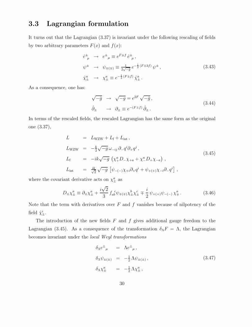
It turns out that the Lagrangian (3.37) is invariant under the following rescaling of fields
by two arbitrary parameters F (x) and f(x):
e±µ → e±µ ≡ eF±f e±µ ,
ψ± → ψ∓(∓) ≡ 12√−g
e−12
(F∓3f) ψ± ,
χa± → χa
± ≡ e−12
(F±f) χa± .
(3.43)
As a consequence, one has:
√−g → √−g = e2F
√−g ,
∂± → ∂± ≡ e−(F±f) ∂± .(3.44)
In terms of the rescaled fields, the rescaled Lagrangian has the same form as the original
one (3.37),
L = LWZW + Lf + Lint ,
LWZW = −k2
√−g ω−ij ∂−qi∂+qj ,
Lf = −ik√−g(χa
+D−χ+a + χa−D+χ−a
),
Lint = ik√2
√−g[ψ−(−)χ+i∂+q
i + ψ+(+)χ−i∂−qi],
(3.45)
where the covariant derivative acts on χa± as
D∓χa± ≡ ∂∓χa
± +i√
2
3f c
abψ∓(∓)χb±χ
c± ∓
i
2ψ+(+)ψ−(−) χ
a∓ . (3.46)
Note that the term with derivatives over F and f vanishes because of nilpotency of the
field χi±.
The introduction of the new fields F and f gives additional gauge freedom to the
Lagrangian (3.45). As a consequence of the transformation δΛF = Λ, the Lagrangian
becomes invariant under the local Weyl transformations
δΛe±
µ = Λe±µ ,
δΛψ±(±) = −12Λψ±(±) ,
δΛχa± = −1
2Λχa
± ,
(3.47)
30
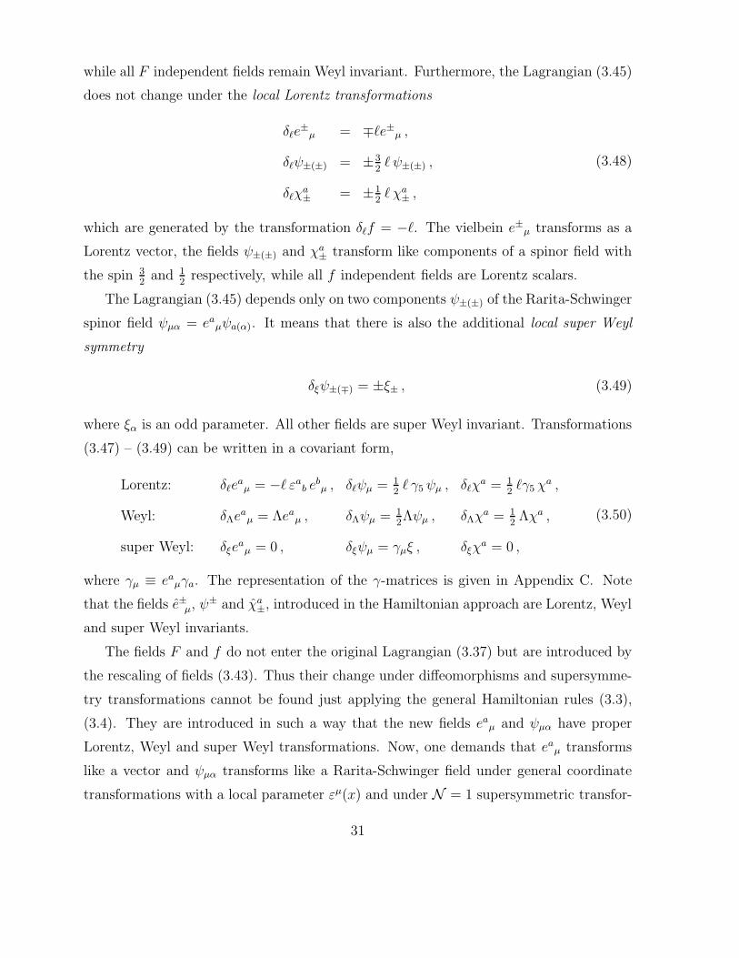
while all F independent fields remain Weyl invariant. Furthermore, the Lagrangian (3.45)
does not change under the local Lorentz transformations
δ`e±
µ = ∓`e±µ ,
δ`ψ±(±) = ±32` ψ±(±) ,
δ`χa± = ±1
2` χa
± ,
(3.48)
which are generated by the transformation δ`f = −`. The vielbein e±µ transforms as a
Lorentz vector, the fields ψ±(±) and χa± transform like components of a spinor field with
the spin 32
and 12
respectively, while all f independent fields are Lorentz scalars.
The Lagrangian (3.45) depends only on two components ψ±(±) of the Rarita-Schwinger
spinor field ψµα = eaµψa(α). It means that there is also the additional local super Weyl
symmetry
δξψ±(∓) = ±ξ± , (3.49)
where ξα is an odd parameter. All other fields are super Weyl invariant. Transformations
(3.47) – (3.49) can be written in a covariant form,
Lorentz: δ`eaµ = −` εa
b ebµ , δ`ψµ = 1
2` γ5 ψµ , δ`χ
a = 12`γ5 χ
a ,
Weyl: δΛeaµ = Λea
µ , δΛψµ = 12Λψµ , δΛχ
a = 12Λχa ,
super Weyl: δξeaµ = 0 , δξψµ = γµξ , δξχ
a = 0 ,
(3.50)
where γµ ≡ eaµγa. The representation of the γ-matrices is given in Appendix C. Note
that the fields e±µ, ψ± and χa±, introduced in the Hamiltonian approach are Lorentz, Weyl
and super Weyl invariants.
The fields F and f do not enter the original Lagrangian (3.37) but are introduced by
the rescaling of fields (3.43). Thus their change under diffeomorphisms and supersymme-
try transformations cannot be found just applying the general Hamiltonian rules (3.3),
(3.4). They are introduced in such a way that the new fields eaµ and ψµα have proper
Lorentz, Weyl and super Weyl transformations. Now, one demands that eaµ transforms
like a vector and ψµα transforms like a Rarita-Schwinger field under general coordinate
transformations with a local parameter εµ(x) and under N = 1 supersymmetric transfor-
31
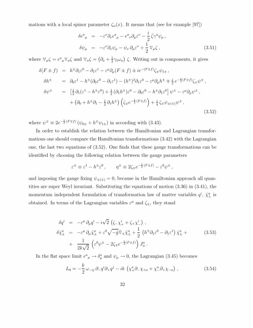
mations with a local spinor parameter ζα(x). It means that (see for example [97])
δeaµ = −εν∂νe
aµ − ea
ν∂µεν − i
2ζγaψµ ,
δψµ = −εν∂νψµ − ψν ∂µεν +
1
2Oµζ , (3.51)
where Oµζ = eaµOaζ and Oaζ =
(∂a + 1
2γ5ωa
)ζ . Writing out in components, it gives
δ(F ± f) = h±∂1ε0 − ∂1ε
1 − εµ∂µ(F ± f)± ie−(F±f)ζ∓ψ1∓ ,
δh± = ∂0ε1 − h±(∂0ε
0 − ∂1ε1)− (h±)2∂1ε
0 − εµ∂µh± ∓ i
2e−
12(F±f)ζ∓ψ± ,
δψ± =[
12∂1(ε
1 − h±ε0) + 12(∂1h
±)ε0 − ∂0ε0 − h±∂1ε
0]ψ± − εµ∂µψ
± ,
+(∂0 + h±∂1 − 1
2∂1h
±) (ζ∓e− 12
(F±f))
+ i4ζ∓ψ±(∓)ψ
± ,
(3.52)
where ψ∓ ≡ 2e−12
(F∓f) (ψ0± + h∓ψ1±) in according with (3.43).
In order to establish the relation between the Hamiltonian and Lagrangian transfor-
mations one should compare the Hamiltonian transformations (3.42) with the Lagrangian
one, the last two equations of (3.52). One finds that these gauge transformations can be
identified by choosing the following relation between the gauge parameters
ε± ≡ ε1 − h±ε0 , η± ≡ 2ζ∓e−12
(F±f) − ε0ψ± ,
and imposing the gauge fixing ψ±(∓) = 0, because in the Hamiltonian approach all quan-
tities are super Weyl invariant. Substituting the equations of motion (3.36) in (3.41), the
momentum independent formulation of transformation law of matter variables qi, χa± is
obtained. In terms of the Lagrangian variables εµ and ζ±, they stand
δqi = −εµ ∂µqi − i√
2(ζ−χi
+ + ζ+χi−),
δχa± = −εµ ∂µχ
a± + ε0
√−gO∓χa
± +1
2
(h±∂1ε
0 − ∂1ε1)χa± + (3.53)
+1
2k√
2
(ε0ψ± − 2ζ∓e−
12(F±f)
)Ja± .
In the flat space limit eaµ → δa
µ and ψµ → 0, the Lagrangian (3.45) becomes
L0 = −k2ω−ij ∂−qi∂+q
j − ik(χa
+∂−χ+a + χa−∂+χ−a
), (3.54)
32
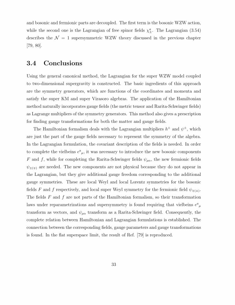
and bosonic and fermionic parts are decoupled. The first term is the bosonic WZW action,
while the second one is the Lagrangian of free spinor fields χa±. The Lagrangian (3.54)
describes the N = 1 supersymmetric WZW theory discussed in the previous chapter
[79, 80].
3.4 Conclusions
Using the general canonical method, the Lagrangian for the super WZW model coupled
to two-dimensional supergravity is constructed. The basic ingredients of this approach
are the symmetry generators, which are functions of the coordinates and momenta and
satisfy the super KM and super Virasoro algebras. The application of the Hamiltonian
method naturally incorporates gauge fields (the metric tensor and Rarita-Schwinger fields)
as Lagrange multipliers of the symmetry generators. This method also gives a prescription
for finding gauge transformations for both the matter and gauge fields.
The Hamiltonian formalism deals with the Lagrangian multipliers h± and ψ±, which
are just the part of the gauge fields necessary to represent the symmetry of the algebra.
In the Lagrangian formulation, the covariant description of the fields is needed. In order
to complete the vielbeins eaµ, it was necessary to introduce the new bosonic components
F and f , while for completing the Rarita-Schwinger fields ψµα, the new fermionic fields
ψ±(∓) are needed. The new components are not physical because they do not appear in
the Lagrangian, but they give additional gauge freedom corresponding to the additional
gauge symmetries. These are local Weyl and local Lorentz symmetries for the bosonic
fields F and f respectively, and local super Weyl symmetry for the fermionic field ψ∓(±).
The fields F and f are not parts of the Hamiltonian formalism, so their transformation
laws under reparametrizations and supersymmetry is found requiring that vielbeins eaµ
transform as vectors, and ψµα transform as a Rarita-Schwinger field. Consequently, the
complete relation between Hamiltonian and Lagrangian formulations is established. The
connection between the corresponding fields, gauge parameters and gauge transformations
is found. In the flat superspace limit, the result of Ref. [79] is reproduced.
33
Chapter 4
Irregular constrained systems
In the previous chapters, the Hamiltonian analysis was used to find all local symmetries of
the WZW model and its supersymmetric extension. The canonical method was applied to
construct the super WZW action coupled to supergravity, starting from the representation
of the super Virasoro algebra.
In general, Dirac’s Hamiltonian analysis provides a systematic technique for finding
the gauge symmetries and the physical degrees of freedom of constrained systems like
gauge theories and gravity [59]. These theories contain more dynamical variables than is
minimally requested by physics and, consequently, they are not independent. Therefore,
in those theories constraints arise as functions of local coordinates in phase space, and
they are usually functionally independent, at least in the most common cases of physical
interest. However, there are some exceptional cases in which functional independence is
violated, when it is not always clear how to identify local symmetries and physical degrees
of freedom. In this chapter, these irregular systems are analyzed. For the review of the
Hamiltonian formalism see Appendix A.
4.1 Regularity conditions
Consider a constrained system on phase space Γ with local coordinates zn = (q, p)
(n = 1, . . . , 2N) and a complete set of constraints
φr (z) ≈ 0 , (r = 1, . . . , R) , (4.1)
34
which define a constraint surface1
Σ = z ∈ Γ | φr(z) = 0 (r = 1, . . . , R) (R ≤ 2N) . (4.2)
Dirac’s procedure guarantees that the system remains on the constraint surface during
its evolution.
Choosing different coordinates on Γ may lead to different forms for the constraints
whose functional independence is not obvious. The regularity conditions (RCs) were
introduced by Dirac to test this [98]:
The constraints φr ≈ 0 are regular if and only if their small variations δφr evaluated
on Σ define R linearly independent functions of δzn.
To first order in δzn, the variations of the constraints have the form
δφr = Jrn δzn , (r = 1, ..., R) , (4.3)
where Jrn ≡ ∂φr/∂zn|Σ is the Jacobian evaluated on the constraint surface. An equivalent
definition of the RCs is [99]:
The set of constraints φr ≈ 0 is regular if and only if the Jacobian Jrn = ∂φr/∂zn|Σ
has maximal rank, <(J) = R .
A system of just one constraint can also fail the test of regularity, as for the con-
straint φ = q2 ≈ 0 in a 2-dimensional phase space (q, p). In this case, the Jacobian
J = (2q, 0)q2=0 = 0 has zero rank. The same problem occurs with the constraint qk ≈ 0,
for k > 1, which has a zero of k-th order on the constraint surface. Thus one constraint
may be dependent on itself, while one function is, by definition, always functionally inde-
pendent.
Equivalent constraints. Different sets of constraints are said to be equivalent if
they define the same constraint surface. This definition refers to the locus of constraints,
not to the equivalence of the resulting dynamics. Since the surface Σ is defined by the
1This terminology is standard in Hamiltonian analysis although, in general, the set Σ is not a manifold
since it can contain discontinuities, be non-differentiable, etc.
35
zeros of the constraints, while the regularity conditions depend on their derivatives, it is
possible to replace a set of irregular φ’s by an equivalent set of regular constraints φ.
In the following sections, the nature of the constraints that give rise to irregularity is
analyzed, and where the irregularities can occur.
4.2 Basic types of irregular constraints
Irregular constraints can be classified according to their behavior in the vicinity of the
surface Σ. For example, linearly dependent constraints have Jacobian with constant rank
R′ throughout Σ, and
φr ≡ Jrn(z) (zn − zn) ≈ 0 , <(J) = R′ < R . (4.4)
These constraints are regular systems in disguise simply because R − R′ constraints are
redundant and should be discarded. The subset with R′ linearly independent constraints
gives the correct description. For example, linearly dependent constraints are clearly in
this category. Apart from this trivial case, two main types of truly irregular constraints,
which do not possess a linear approximation in the vicinity of some points of Σ, can be
distinguished:
Type I. Multilinear constraints. Consider the constraint
φ ≡M∏i=1
fi(z) ≈ 0 , (4.5)
where the functions fi have simple zeros. Each factor defines a surface of codimension 1,
Σi ≡ z ∈ Γ | fi(z) = 0 , (4.6)
and Σ is the collection of all surfaces, Σ =⋃
Σi. The rank of the Jacobian of φ is reduced
at intersections
Σij ≡ Σi
⋂Σj . (4.7)
Thus, the RCs hold everywhere on Σ, except at the intersections Σij , where φ has zeros
of higher order. Note that the intersections (4.7) also include the points where more than
two Σ’s overlap.
36
Type II. Nonlinear constraints. Consider the constraint of the form
φ ≡ [f(z)]k ≈ 0 , (k > 1) , (4.8)
where the function f(z) has a simple zero. This constraint has a zero of order k in the
vicinity of Σ, its Jacobian vanishes on the constraint surface and, therefore, the RCs fail2.
It could seem harmless to replace φ by the equivalent regular constraint f(z) ≈ 0, but
it is allowed to do only if it does not change the dynamics of original system, what is
discussed below.
Types I and II are the two fundamental generic classes of irregular constraints. In
general, there can be combinations of them occurring simultaneously near a constraint
surface, as in constraints of the form φ = [f1(z)]2 f2(z) ≈ 0, etc.
4.3 Classification of constraint surfaces
The previous classification refers to the way in which φ approaches zero. Now it is going
to be discussed where regularity can be violated.
The example of q2 ≈ 0 showed that only one constraint can be irregular, even if, as a
function, it is functionally independent. This is possible since functional independence of
the functions φr(z) permits the Jacobian ∂φr/∂zi to have rank lower than maximal on a
submanifold of measure zero,
Ξ =
w ∈ Γ
∣∣∣∣<(∂φr
∂zi
)z=w
< R
, (4.9)
while the constraints φr ≈ 0 have the Jacobian evaluated at the particular surface Σ.
Their intersection
Σ0 = Σ ∩ Ξ (4.10)
defines a submanifold on Σ where the RCs are violated, while on the rest of Σ the RCs
are satisfied.
Thus, barring accidental degeneracies such as linearly dependent constraints, one of
these three situation may present themselves:
2Here it is assumed k > 1, in order to avoid infinite values for ∂φ∂zi on Σ.
37
A. The RCs are satisfied everywhere on the constraint surface: The surfaces Σ and Ξ
do not intersect and J has maximal rank throughout Σ. These are regular systems.
B. The RCs fail everywhere on the constraint surface: Σ0 = Σ is a submanifold of Ξ and
J has constant rank R′ < R on Σ0. This irregular system contains nonlinear (type
II) constraints.
C. The RCs fail on Σ0: The intersection Σ0 is a measure zero submanifold on Σ, so that
< (J) = R′ < R on Σ0, while < (J) = R elsewhere on Σ. This irregular system
contains multilinear (type I) constraints.
In the last case, the constraint surface can be decomposed into two non overlapping
sets Σ0 and ΣR. Then, the rank of the Jacobian jumps from < (J) = R on ΣR, to
< (J) = R′ on Σ0 and the manifold Σ is not differentiable at Σ0. Although the functions
φr are continuous and differentiable, this is not sufficient for regularity.
For example, a massless relativistic particle in Minkowski space has phase space (qµ, pν)
with both regular and irregular sectors. The constraint φ ≡ pµpµ ≈ 0 has Jacobian
J = (0, 2pµ)φ=0, and its rank is one everywhere, except at the apex of the cone, pµ = 0,
where the light-cone is not differentiable and the Jacobian has rank zero. From the
viewpoint of irreducible representations of the Poincare group, the orbits with pµ = 0
correspond to the trivial representation of the group, and this point is excluded from the
phase space of the massless particle (see, e.g., [100]).
The lack of regularity, however, is not necessarily due to the absence of a well defined
smooth tangent space for Σ. Consider for example the multilinear constraint
φ(x, y, z) = (x− 1)(x2 + y2 − 1) ≈ 0 . (4.11)
Here the constraint surface Σ is composed of two sub-manifolds: the plane Π = (x, y, z) |x− 1 ≈ 0, and the cylinder C = (x, y, z) | x2 + y2 − 1 ≈ 0, which are tangent to each
other along the line L = (x, y, z) | x = 1, y = 0, z ∈ R. The Jacobian on Σ is
J =(3x2 + y2 − 2x− 1, 2y (x− 1) , 0
)φ=0
, (4.12)
and its rank is one everywhere, except on L, where it is zero. The constraint φ is irregular
on this line. However, the tangent vectors to Σ are well defined there. The irregularity
38
arises because φ is a multilinear constraint of the type described by (4.5) and has two
simple zeros overlapping on L. The equivalent set of regular constraints on L is φΠ =
x− 1 ≈ 0, φC = x2 + y2 − 1 ≈ 0.
4.4 Treatment of systems with multilinear constraints
In what follows regular systems and linearly dependent constraints will not be discussed.
They are either treated in standard texts, or they can be trivially reduced to the regular
case.
Consider a system of type I, as in Eq. (4.5). In the vicinity of an irregular point where
only two surfaces (4.6) intersect, say Σ1 and Σ2, the constraint φ ≈ 0 is equivalently
described by the set of regular constraints
f1 ≈ 0 , f2 ≈ 0 . (4.13)
This replacement generically changes the Lagrangian of the system, and the orbits, as
well. Suppose the original canonical Lagrangian is
L(q, q, u) = piqi −H(q, p)− uφ(q, p) , (4.14)
where H is the Hamiltonian containing all regular constraints. Replacing φ by (4.13),
gives rise to an effective extended Lagrangian
L12(q, q, v) = piqi −H(q, p)− v1f1(q, p)− v2f2(q, p) . (4.15)
defined on Σ12. Thus, instead of the irregular Lagrangian (4.14) defined on the whole
Σ, there is a collection of regularized effective Lagrangians defined in the neighborhood
of the different intersections of Σis. For each of these regularized Lagrangians, the Dirac
procedure can be carried out to the end.
This can be illustrated with the example of a Lagrangian in a (2 +N)-dimensional
configuration space (x, y, q1, . . . , qN),
L =1
2
N∑k=1
(qk)2
+1
2
(x2 + y2
)− λxy . (4.16)
39
This Lagrangian describes a free particle moving on the set(x, y, qk
)∈ R
N+2∣∣ xy = 0
⊂
RN+2, which is the union of two (N + 1)-dimensional planes where x and y vanish re-
spectively. The constraint surface defined by xy = 0 can be divided into the following
sets:
Σ1 =(x, 0, qk; px, py, pk
)∣∣ x 6= 0,
Σ2 =(
0, y, qk; px, py, pk
)∣∣ y 6= 0, (4.17)
Σ12 =(
0, 0, qk; px, py, pk
).
The constraint is regular on Σ1
⋃Σ2, while on Σ12 it is irregular and can be exchanged
by φ1 = x ≈ 0, φ2 = y ≈ 0. The corresponding regularized Lagrangians are
L1 =1
2
N∑k=1
(qk)2
+1
2x2 ,
L2 =1
2
N∑k=1
(qk)2
+1
2y2 , (4.18)
L12 =1
2
N∑k=1
(qk)2,
and the Lagrange multipliers have dropped out, so the regularized Lagrangians describe
physical degrees of freedom only – as expected.
The corresponding regularized Hamiltonians are
H1 =1
2
N∑k=1
p2k +
1
2p2
x ,
H2 =1
2
N∑k=1
p2k +
1
2p2
y , (4.19)
H12 =1
2
N∑k=1
p2k ,
which are defined in the corresponding reduced manifolds of phase space (obtained after
completing the Dirac-Bergman procedure):
Σ1 =(x, 0, qk; px, 0, pk
)∣∣ x 6= 0,
Σ2 =(
0, y, qk; 0, py, pk
)∣∣ y 6= 0, (4.20)
Σ12 =(
0, 0, qk; 0, 0, pk
).
40
It is straightforward to generalize the proposed treatment when more than two surfaces
Σi overlap.
Evolution of a multilinearly constrained system. In the presence of a multilin-
ear constraint, there are regions of the phase space where the Jacobian has different rank.
A question is, whether the system can evolve from a generic configuration in a region of
maximal rank, to a configuration of lower rank, in finite time, and in the case that that
were possible, what happens with the system afterwards.
To answer this question, consider the example (4.16) for N = 1,
L =1
2
(x2 + y2 + z2
)− λxy . (4.21)
In the regions Σ1 and Σ2 [see Eqs. (4.17)], the rank is maximal and the free particle can
move freely along the x- or y-axis, respectively.
Suppose that the initial state is
x(0) = a > 0 , y(0) = 0 , z(0) = 0 , x(0) = −v < 0 , y(0) = 0 , z(0) = 0 ,
(4.22)
so that the particle is moving on Σ1, with finite speed along the x-axis towards x = 0
on Σ12. The evolution is given by x(t) = a − vt, y(t) = 0, z(t) = 0 and the particle
clearly reaches x = 0 in a finite time (T = a/v). What happens then? According to
the evolution equation, for x < 0 the trajectory takes the form x(t) = a′ − v′t, y(t) = 0,
z(t) = 0, however the action would be infinite unless a = a′ and v = v′. Therefore, the
particle continues unperturbed past beyond the point where the RCs fail. So, the irregular
surface is not only reachable in a finite time, but it is crossed without any observable effect
on the trajectory.
From the point of view of the trajectory in phase space, it is clear that the initial
state (a, 0, 0;−v, 0, 0) lies on the surface Σ1, and at t = T the system reaches the point
(0, 0, 0;−v, 0, 0), which does not lie on the surface Σ12 = (0, 0, z; 0, 0, pz).While it is true that at t = T the Jacobian changes rank, it would be incorrect to
conclude that the evolution suffers a jump since the dynamical equations are perfectly
valid there. In order to have a significant change in the dynamics, the Jacobian should
change its rank in an open set.
41
Degenerate systems. The problem of evolution in irregular systems should not be
confused with the issues arising in degenerate systems, in which the symplectic matrix of
regular constraints φr, φs = Ωrs (z) is a phase space function which changes its rank at
t = τ . In those systems, it is possible for a system in a generic initial configuration, to
reach (in a finite time) a configuration where the symplectic form Ωrs (z (τ)) has lower
rank, leading to a new gauge invariance which cancels a number of degrees of freedom
[67, 68].
That problem is unrelated to the one discussed in irregular systems and can be treated
independently. In the irregular case it is the functional independence of the constraints
that fails; in the degenerate dynamical systems it is the symplectic structure that breaks
down.
4.5 Systems with nonlinear constraints
Consider the case of irregular systems of type II. It will be shown that a nonlinear irregular
constraint can be replaced by an equivalent linear one without changing the dynamical
contents of the theory, provided the linear constraint is second class. Otherwise, the
resulting Hamiltonian dynamics will be, in general, inequivalent to that of the original
Lagrangian system.
In order to illustrate this point, consider a system given by the Lagrangian
L(q, q, u) =1
2γij q
iqj − u [f(q)]k , (4.23)
where k > 1 and
f(q) ≡ ciqi 6= 0, i = 1, ..., N . (4.24)
Here it is assumed that the metric γij to be constant and invertible, and the coefficients
ci are also constant. The Euler-Lagrange equations describe a free particle in an N -
dimensional space, with time evolution qi(t) = vi0 t+q
i0, where u(t) is a Lagrange multiplier.
This solution is determined by 2N initial conditions, qi(0) = qi0 and qi(0) = vi
0 subject to
the constraints ciqi0 = 0 and civ
i0 = 0. Thus, the system possesses N − 1 physical degrees
of freedom.
42
In the Hamiltonian approach this system has a primary constraint π ≡ ∂L∂u≈ 0 whose
preservation in time leads to the secondary constraint
φ ≡ [f(q)]k ≈ 0 . (4.25)
According to (4.8), this is a nonlinear constraint and there are no further constraints. As
a consequence, the system has only two first class constraintsπ ≈ 0, fk ≈ 0
, and N−1
degrees of freedom, as found in the Lagrangian approach.
On the other hand, if one chooses instead of (4.25), the equivalent linear constraint
f(q) = ciqi ≈ 0 , (4.26)
then its time evolution yields a new constraint,
χ(p) ≡ γijci pj ≈ 0 . (4.27)
Now, since
f, χ = γijci cj ≡ ‖c‖2 , (4.28)
two cases can be distinguished:
• If ‖c‖ = 0, there are three first class constraints, π ≈ 0, f ≈ 0 and χ ≈ 0,
which means that the system has N − 2 physical degrees of freedom. In this case,
substitution of (4.25) by the equivalent linear constraint (4.26), yields a dynamically
inequivalent system3.
• If ‖c‖ 6= 0, then f ≈ 0 and χ ≈ 0 are second class, while π ≈ 0 is first class, which
leaves N − 1 physical degrees of freedom and the substitution does not change the
dynamics of the system.
Thus, if fk ≈ 0 is irregular, replacing it by the regular constraint f ≈ 0 changes the
dynamics if f is a first class function, but it gives the correct result if it is a second class
function.
3The expression “substitution of constraints” always refers to two steps: (i) the exchange of a set of
constraints by an equivalent set, and (ii) the introduction of a corresponding effective Lagrangian of type
(4.15).
43

Note that in the Lagrangian description there is no room to distinguish first and
second class constraints, so it would seem like the value of ||c|| didn’t matter. However,
the inequivalence of the substitution can be understood in the Lagrangian analysis as
well. Suppose that it were permissible to exchange the constraint fk ≈ 0 by f ≈ 0 in the
Lagrangian. Then, instead of (4.23), one would have
L(q, u) =1
2γij q
iqj − uf(q) . (4.29)
It can be easily checked that (4.29) yields N − 2 degrees of freedom when ‖c‖ = 0, and
N − 1 degrees of freedom when ‖c‖ 6= 0, which agrees with the results obtained in the
Hamiltonian analysis. Note that the substitution of fk by f modifies the dynamics only if
γijci cj = 0, but this can happen nontrivially only if the metric γij is not positive definite.
In general, a nonlinear irregular constraint φ ≈ 0 has a multiple zero on the constraint
surface Σ, which means that its gradient vanishes on Σ as well. An immediate consequence
of ∂φ∂zi ≈ 0, is that φ commutes with all finite functions on Γ,
φ, F (z) ≈ 0 . (4.30)
As a consequence, φ ≈ 0 is first class and is always preserved in time, φ ≈ 0 . On the other
hand, a nonlinear constraint cannot be viewed as a symmetry generator simply because
it does not generate any transformation,
δεzi =
zi, εφ
≈ 0 . (4.31)
Consistently with this, φ cannot be gauge-fixed, as there is no finite function P on Γ such
that φ,P 6= 0 .
In this sense, a nonlinear first class constraint that cannot be gauge-fixed, cancels
only half a degree of freedom. The other half degree of freedom cannot be cancelled
because the gauge-fixing function does not exist and, in particular, it cannot appear
in the Hamiltonian. Although it allow counting the degrees of freedom in a theory,
these systems are pathological and their physical relevance is questionable since their
Lagrangians cannot be regularized.
When a nonlinear constraint φ ≈ 0 can be exchanged by a regular one, the Lagrangian
is regularized as in the case of multilinear constraints. For example, the system (4.23)
44

with ‖c‖ 6= 0 has Hamiltonian
H =1
2γijpipj + λπ + uf(q) , (4.32)
where f = ciqi will turn out to be a second class constraint. The corresponding regularized
Lagrangian coincides with L, Eq. (4.29), as expected.
In Refs. [61, 63] irregular systems of the type II were discussed. It was pointed out
that there was a possible loss of dynamical information in some cases. From our point of
view, it is clear that this would occur when f is a first class function.
4.6 Some implications of the irregularity
a) Linearization
It has been observed in five dimensional Chern-Simons theory, that the effective action for
the linearized perturbations of the system around certain backgrounds seems to have more
degrees of freedom than the fully nonlinear theory [58]. This is puzzling since the heuristic
picture is that the degrees of freedom of a system correspond to the small perturbations
around a local minimum of the action, and therefore the number of degrees of freedom
should not change when the linearized approximation is used.
In view of the discussion in the previous section, it is clear that a possible solution of
the puzzle lies in the fact that substituting a nonlinear constraint by a linear one may
change the dynamical features of the theory. But the problem with linear approximations
is more serious: the linearized approximation retains only up to quadratic and bilinear
terms in the Lagrangian, which give linear equations for the perturbations. Thus, irregular
constraints in the vicinity of the constraint surface are erased in the linearized action. The
smaller number of constraints in the effective theory can lead to the wrong conclusion that
the effective system possess more degrees of freedom than the unperturbed theory. The
lesson to be learned is that the linear approximation is not valid in the part of the phase
space where the RCs fail.
This is illustrated by the same example discussed earlier (4.23). One can choose as a
45
background the solution (q1, . . . , qN , u), where qi(t) = qi0 + vi
0t satisfies the constraint
ciqi = 0 , (4.33)
and u(t) is an arbitrarily given function. This describes a free particle moving in the
(N − 1)-dimensional plane defined by (4.33). The linearized effective Lagrangian, to
second order in the small perturbations si = qi − qi(t) and w = u− u(t), has the form
Leff (s, w) =1
2γij
(vi0 + si
) (vj0 + sj
)− u
(cis
i)2, (4.34)
and the equations of motion are
si + Γij(t) s
j = 0 , (i = 1, . . . , N) , (4.35)
where Γij ≡ 2u γikckcj is the eigen-frequency matrix. Since u is not a dynamical variable,
it is not varied and the nonlinear constraint (cisi)
2= 0 is absent from the linearized
equations. The system described by (4.35) possesses N physical degrees of freedom, that
is, one degree of freedom more than the original nonlinear theory (4.23).
The only indication that one of these degrees of freedom has a nonphysical origin is
the following: If ‖c‖ 6= 0, splitting the components of si along ci and orthogonal to ci as
si(t) ≡ s(t)γijcj + si⊥(t) , (4.36)
gives rise to the projected equations
si⊥ = 0 , (4.37)
s+ 2u(t)‖c‖2s = 0 . (4.38)
The N − 1 components of si⊥(t) obey a deterministic second order equation, whereas s(t)
satisfies an equation which depends on an indeterminate arbitrary function u(t). The
dependence of s = s(t, u(t)) on the background Lagrange multiplier u is an indication
that s is a nonphysical degree of freedom, since u was an arbitrary function to begin with.
This is not manifest in Eq. (4.38), where u is a fixed function and, from a naive point of
view, s(t) is determined by the same equation, regardless of the physically obscure origin
of the function u. It is this naive analysis that leads to the wrong conclusion indicated
above.
46
Note that a linearized theory may be consistent by itself, but it is not necessarily a
faithful approximation of a nonlinear theory.
One way to avoid the inconsistencies between the original theory and the linearized
one would be to first regularize the constraints (if possible) and then linearize the corre-
sponding regular Lagrangian.4
b) Dirac conjecture
Dirac conjectured that all first class constraints generate gauge symmetries. It was shown
that Dirac’s conjecture is not true for first class constraints of the form fk (k > 1), and
following from f ≈ 0 [101, 102]. Therefore, for systems with nonlinear constraints, the
conjecture does not work and they generically provide counterexamples of it [99, 109, 110].
From the point of view of irregular systems, it is clear that Dirac’s conjecture fails
for nonlinear constraints because they do not generate any local transformation, c.f. Eq.
(4.31). In Refs. [61, 63] it was observed that Dirac’s conjecture may not hold in the
presence of irregular constraints of type II.
In the case of multilinear constraints, however, Dirac’s conjecture holds. The fact that
at irregular points the constraints do not generate any transformation only means that
these are fixed points of the gauge transformation.
c) Quantization
Although it is possible to deal systematically with classical theories containing irregular
constraints, there may be severe problems in their quantum description. Consider a path
integral of the form
Z ∼∫
[dq][dp][du] exp i [pq −H(q, p)− uφ(q, p)] , (4.39)
where φ = [f(q, p)]k is a nonlinear constraint. Integration on u yields to δ(fk), which
is not well-defined for a zero of order k > 1, making the quantum theory ill defined.
Only if the nonlinear constraint could be exchanged by the regular one, f(q, p) ≈ 0, the
4There may be also other problems in linear approximation (e.g., when a topology is non-trivial), but
these cases are not discussed here.
47
quantum theory could be saved. An example of this occurs in the standard approach
for QED, where it is usual practice to introduce the nonlinear (Coulomb) gauge fixing
term u(∂iAi)2 in order to fix the Gauss law φ = ∂iπ
i ≈ 0 (where πi ≡ δIED
δAi). Since the
function f(A) = ∂iAi is second class, the substitution of f 2 (A) ≈ 0 by a regular constraint
f (A) ≈ 0 does not change its dynamical structure.
The other possibility to quantize a system with a nonlinear constraint is to modify
the original Lagrangian so that it becomes regular, leading to the the change in dynamics
as well. This possibility is considered in the Siegel model of the chiral boson [103], whose
quantum theory is analyzed in [104].
There are other examples of irregular systems whose quantum theories are discussed
in the literature. For example, it is shown that for the models of relativistic particles
with higher spin (s > 12), called systems admitting no gauge conditions, since they contain
irregular first class constraints, different quantization methods can lead to different phys-
ical results [105, 106]. Other examples of quantum irregular systems are planar gauge
field theories [107] and topologically massive gauge fields [108].
4.7 Summary
The dynamics of a system possessing constraints which may violate the regularity condi-
tions (functional independence) on some subsets of the constraint surface Σ, was discussed.
These so-called irregular systems are seen to arise generically because of nonlinearities in
the constraints and can be classified into two families: multilinear (type I) and nonlinear
(type II).
• Type I constraints are of the form φ =∏fi(z), where fi possess simple zeros. These
constraints violate the regularity conditions (RCs) on sets of measure zero on the
constraint surface Σ.
• Type I constraints can be exchanged by equivalent constraints which are regular
giving an equivalent dynamical system.
• Type II constraints are of the form φ = fk (k > 1) where f has a simple zero. They
violate the RCs on sets of nonzero measure on Σ.
48
• A type II constraint can be replaced by an equivalent linear one only if the latter is
second class; if the equivalent linear constraint is first class, substituting it for the
original constraint would change the system.
• In general, the orbits can cross the configurations where the RCs are violated without
any catastrophic effect for the system. If the symplectic form degenerates at the
irregular points, additional analysis is required.
• The naive linearized approximation of an irregular constrained system generically
changes it by erasing the irregular constraints. In order to study the perturba-
tions around a classical orbit in an irregular system, it would be necessary to first
regularize it (if possible) and only then do the linearized approximation.
49
Chapter 5
Higher-dimensional Chern-Simons
theories as irregular systems
In this chapter the Hamiltonian dynamics of Chern-Simons (CS) theories in D ≥ 5 is
analyzed. It is known that regular and generic CS theories are invariant under the gauge
symmetries and diffeomorphisms [54, 55], but these theories also possess sectors in phase
space which are irregular [66]. Here a criterion for the choice of a regular background in
CS theories is found, and the implications of the irregularity in CS theories are discussed.
The dynamics arising at the boundary is not considered here.
5.1 Chern-Simons action
A CS theory is one where the fundamental field is a Lie-algebra-valued connection one-
form A = AaGa, where the corresponding anti-Hermitean generators close a N -dimensio-
nal algebra [Ga,Gb] = f cab Ga. The connection field defines a covariant derivative D that
acts on a p-form ω as Dω = dω + [A, ω].1
The CS Lagrangian is a (2n + 1) - form such that its exterior derivative (in 2n + 2
dimensions) is
dLCS = k ga1···an+1 Fa1 · · ·F an+1 . (5.1)
1A p-form is the object ω = 1p! ωn1···np dxn1 · · · dxnp , and the commutator of p-form ω and q-form Ω is
given by [ω, Ω] = ωΩ− (−)pq Ωω.
50

Here k is a dimensionless constant, ga1 ...an+1 is a completely symmetric, invariant tensor
(Dga1···an+1 = 0) and F =F aGa = dA+A2 is the field-strength 2-form which satisfies the
Bianchi identity DF = 0.
The definition (5.1) is based on the fact that the form on the r.h.s. is closed (its exterior
derivative vanishes due to the Bianchi identity) and therefore can locally be written as
dLCS. Applying Stokes’ theorem to (5.1), the integral of the total derivative becomes the
integration over the D-dimensional manifold MD = ∂MD+1 without boundary and one
obtains the integral identity∫MD+1
dLCS(A) =∫MD
LCS(A). In general, a CS theory is
defined on an arbitrary (not necessary closed) manifoldM,
ICS[A] =
∫M
LCS(A) . (5.2)
Variation of the expression (5.1) with respect to the gauge field Aa gives (up to an exact
form)
δLCS = k (n+ 1) gaa1···an Fa1 · · ·F anδAa , (5.3)
from where, supposing the suitable boundary conditions which give a well defined ex-
tremum for ICS, the Euler-Lagrange equations are obtained,
gaa1···an Fa1 · · ·F an = 0 . (5.4)
Written with all indices, the equations of motion are
εµµ1ν1···µnνngaa1···an Fa1µ1ν1· · ·F an
µnνn= 0 , (5.5)
where xµ (µ = 0, 1, . . . , 2n) are local coordinates atM.
The CS action possesses the following local symmetries:
• By construction, it is invariant under general coordinate transformations or diffeo-
morphisms
xµ → x′µ = xµ + ξµ(x) ,
A(x) → A′(x′) = A(x) , (δξA = −£ξA) , (5.6)
where £ξAaµ ≡ ∂µξ
νAaν + ξν∂νA
aµ stands for a Lie derivative;
51
• It has an infinitesimal gauge symmetry,
δλA = −Dλ , (5.7)
since the r.h.s. of (5.1) is an explicitly gauge invariant expression.
Under large gauge transformations, a CS action changes for a closed form. In this
chapter the local dynamics is analyzed, and all effects arising at the boundary are ne-
glected.
5.2 Hamiltonian analysis of Chern-Simons theories
Here the features of the sectors with regular dynamics of (2n+1)-dimensional CS theories
are reviewed, where the dimension is larger than three [55].
In the Hamiltonian approach, one supposes that the space-time manifoldM has topol-
ogy R×σ, where σ is a 2n-dimensional spatial manifold parametrized by local coordinates
xi. The CS action ICS, defined by (5.1) and (5.2), is linear in velocities (first order for-
malism) and can be written as
ICS [A] =
∫d2n+1x
(Li
a Aai − Aa
0χa
), (5.8)
where2
χa ≡ −k
2n(n + 1) εi1j1···injn gaa1···anF
a1i1j1· · ·F an
injn, (5.9)
and εi1···i2n ≡ ε0i1···i2n . The explicit form of Lia is not necessary since it defines the kinetic
term through the symplectic form Ωijab :
Ωijab (x, x′) =
δLjb (x′)
δAai (x)
− δLia (x)
δAbj (x′)
= − kn
2n−1(n+ 1) εiji2j2···injngaba2···anF
a1i2j2· · ·F an
injnδ (x− x′) . (5.10)
2The expression for χa can be obtained directly from (5.3) for a special choice of variations δAa =
δAa0 dt, and the definition χa = − δICS
δAa0
following from (5.8).
52
(For derivation see Appendix D.) This matrix plays a central role in the dynamics of
CS theories, as it will be seen later. The gauge field Aai and its canonically conjugated
momenta πia ≡ δICS/δA
ai defines the phase space Γ, with the basic PB
Aa
i (x) , πjb (x′)
= δj
i δab δ (x− x′) (5.11)
taken at the same time x0 = x′0 = t, where δ (x− x′) stands for a Dirac δ-function at the
spatial section. The field Aa0 is a Lagrange multiplier.
Constraints. Constraints in the theory are
φia ≡ πi
a − Lia(A) ≈ 0 ,
Ga ≡ −χa +Diφia ≈ 0 , (5.12)
where the covariant derivative acts on φia as Diφ
ia ≡ ∂iφ
ia+f c
abAbiφ
ic. The total Hamiltonian
is
H =
∫d2nx
(−Aa
0Ga + uaiφ
ia
), (5.13)
and it depends on N arbitrary functions Aa0 and 2nN arbitrary functions ua
i . Constraints
define the constraint surface Σ ⊂ Γ and they close the following PB algebra:
π0a, all = 0 , Ga,Gb = f c
ab φicδ ,
φia, φ
jb
= Ωij
abδ , Ga, φib = f c
abφicδ ,
(5.14)
with Ωijab(x, x
′) = Ωijab (x) δ (x− x′). The constraints φi
a and Ga evolve as
φia ≈
φi
a, H
= Ωijabu
bj − f c
abφic ≈ Ωij
abubj = 0 , (5.15)
·Ga ≈
π0
a, H
= f cab
(Ab
0Gc − ubiφ
ic
)≈ 0 , (5.16)
and, therefore, there are no new constraints. The equation (5.15) gives restrictions on a
number of multipliers uia, depending on the rank of Ωij
ab.
53
Generic theories. The dynamics of CS theories basically depends on the symplectic
matrix Ωijab. This matrix is degenerate for any CS theory, due to the identity (Appendix
D)
ΩikabF
bkj = −δi
jχa ≈ 0 . (5.17)
Therefore, there are at least 2n zero modes of the symplectic matrix, (Vi)aj = F a
ij .
Among all CS theories based on a gauge group of dimension N , there is a family of
generic theories for which:
(a) the zero modes of Ωijab are the 2n linearly independent vectors (Vi)
aj = F a
ij;
(b) there are no other zero modes and the rank of symplectic matrix is the largest,
< (Ω) = 2n (N − 1) . (5.18)
For D ≥ 5, a CS theory cannot be generic on the whole phase space. For example,
any CS theory possess a pure gauge solution (F = 0) which does not satisfy generic
conditions (a) and (b). Therefore, a generic CS theory is determined by (i) an invariant
tensor ga1···an+1 and (ii) a domain, or a sector of the phase space on which the generic
conditions (a) and (b) are satisfied. This sector can be chosen as an open set around a
solution A of the constraints χ(A) = 0 such that (a) and (b) are fulfilled for F and Ω.
First and second class constraints. In order to separate first from second class
constraints, a (non-singular) transformation of φia has to be made, which diagonalize the
symplectic form in (5.14):
Hi ≡ F aijφ
ja ≈ 0 , θα ≡ Sa
αiφia ≈ 0 , (5.19)
where α = 1, . . . , 2n (N − 1) . The constraints Hi correspond to the zero modes of Ωijab
and satisfy the algebra
Hi (x) ,Hj (x′) =[Hi (x
′) ∂j +Hj (x) ∂i − F aijGa (x)
]δ (x− x′) , (5.20)
thus they are first class. Constraints θα are second class. The explicit form of the tensor
Saαj is not always possible to find, and the condition
< (∆αβ) = 2n(N − 1) , ∆αβ ≡ Saαi
ΩijabS
bβj , (5.21)
54
provides that the only non-vanishing brackets on Σ are
θα, θβ ≈ ∆αβ δ . (5.22)
Therefore, in a generic CS theory with 2nN dynamical fields Aia, N first class con-
straints Ga, 2n first class constraints Hi , and 2n (N − 1) second class constraints θα, the
number of physical degrees of freedom is:
f2n+1(N) = nN − n−N , (n,N > 1) . (5.23)
Local symmetries. A CS theory is invariant under the following local transforma-
tions:
• Gauge transformations, generated by
G [λ] ≡∫d2nxλaGa , (5.24)
which act on gauge fields as
δλAai = Aa
i , G [λ] = −Diλa ; (5.25)
• Improved spatial diffeomorphisms, generated by
H [ε] ≡∫d2nx εiHi , (5.26)
which change the gauge field as
δεAai = Aa
i ,H [ε] = εjF aji . (5.27)
Local symmetries which are not independent from the above ones, are spatial diffeo-
morphisms, which differ from improved spatial diffeomorphisms by a gauge transforma-
tion,
δξAai = −£ξA
ai = −ξjF a
ji −Di
(ξiAa
i
), (5.28)
and (improved) time reparametrizations, which change the gauge fields as
δεAai = ε0F a
0i . (5.29)
Due to the equations of motion ΩijabF
b0j = 0, the vector F a
0j must be a linear combination
of zero modes of Ωijab, therefore in a generic theory F a
0i = CjF aji. In consequence, the
time-like diffeomorphisms can be obtained from spatial diffeomorphisms on-shell through
the redefinition of local parameter εi = ε0Ci.
55
Non-generic theories. The above analysis can be easily generalized to degenerate
(non-generic) theories, in which the symplectic matrix Ωijab has K independent zero modes
(Uρ)ai = Ua
ρi,
ΩijabU
bρj ≈ 0 , (ρ = 1, . . . , K) (2n < K ≤ 2nN) , (5.30)
where K = 2n corresponds to the generic case. Then the first class constraints are
Hρ ≡ Uaρ jφ
ia ≈ 0 , (5.31)
which, apart from 2n improved spatial diffeomorphisms also generate an additional (K−2n)-parameter symmetry. The number of physical degrees of freedom is given by
f2n+1(N) = nN −N − K
2, (n,N > 1) . (5.32)
This formula is a generalization of (5.23) obtained for generic theories, and it enables
the counting of the degrees of freedom in the sectors of phase space which have more
than minimal number of local symmetries. However, during its evolution, the degenerate
system can change the number of degrees the freedom (loosing them) if it reaches the
point where the symplectic form has lower rank [67, 68]. Therefore, the formula (5.32) is
valid only on an open set not containing degenerate points.
5.3 Regularity conditions
In the previous chapter it was implicitly supposed that all constraints were regular. Now
the regularity conditions in CS theories are going to be analyzed.
First, consider the original set of constraints obtained from Dirac-Bergman algorithm,
φia ≈ 0 and χa ≈ 0. Constraints φi
a are regular since they are linear in momenta. Thus,
the regularity of CS theories is determined by momentum-independent constraints χa. It
is convenient to write χa in the basis of spatial 1-forms dxi as
Ka ≡ d2nxχa = −k (n + 1) gaa1···anFa1 · · ·F an ≈ 0 . (5.33)
Their small variations evaluated at Ka = 0 are
δKa = JabDδAb , (5.34)
56
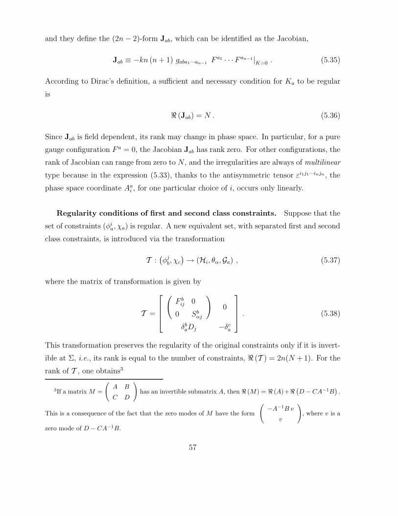
and they define the (2n− 2)-form Jab, which can be identified as the Jacobian,
Jab ≡ −kn (n+ 1) gaba1···an−1 Fa1 · · ·F an−1 |K=0 . (5.35)
According to Dirac’s definition, a sufficient and necessary condition for Ka to be regular
is
< (Jab) = N . (5.36)
Since Jab is field dependent, its rank may change in phase space. In particular, for a pure
gauge configuration F a = 0, the Jacobian Jab has rank zero. For other configurations, the
rank of Jacobian can range from zero to N , and the irregularities are always of multilinear
type because in the expression (5.33), thanks to the antisymmetric tensor εi1j1···injn, the
phase space coordinate Aai , for one particular choice of i, occurs only linearly.
Regularity conditions of first and second class constraints. Suppose that the
set of constraints (φia, χa) is regular. A new equivalent set, with separated first and second
class constraints, is introduced via the transformation
T :(φj
b, χc
)→ (Hi, θα,Ga) , (5.37)
where the matrix of transformation is given by
T =
(F b
ij 0
0 Sbαj
)0
δbaDj −δc
a
. (5.38)
This transformation preserves the regularity of the original constraints only if it is invert-
ible at Σ, i.e., its rank is equal to the number of constraints, < (T ) = 2n(N + 1). For the
rank of T , one obtains3
3If a matrix M =
(A B
C D
)has an invertible submatrix A, then < (M) = < (A)+<
(D − CA−1B
).
This is a consequence of the fact that the zero modes of M have the form
(−A−1B v
v
), where v is a
zero mode of D − CA−1B.
57
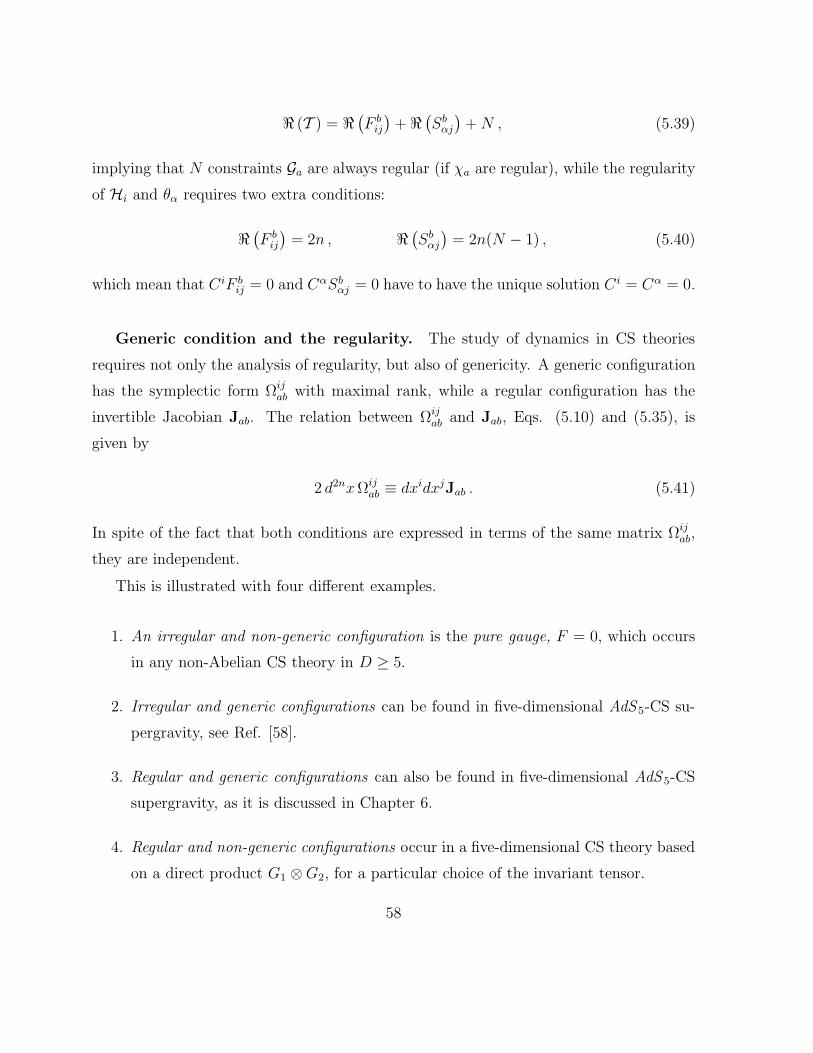
< (T ) = <(F b
ij
)+ <
(Sb
αj
)+N , (5.39)
implying that N constraints Ga are always regular (if χa are regular), while the regularity
of Hi and θα requires two extra conditions:
<(F b
ij
)= 2n , <
(Sb
αj
)= 2n(N − 1) , (5.40)
which mean that CiF bij = 0 and CαSb
αj = 0 have to have the unique solution Ci = Cα = 0.
Generic condition and the regularity. The study of dynamics in CS theories
requires not only the analysis of regularity, but also of genericity. A generic configuration
has the symplectic form Ωijab with maximal rank, while a regular configuration has the
invertible Jacobian Jab. The relation between Ωijab and Jab, Eqs. (5.10) and (5.35), is
given by
2 d2nxΩijab ≡ dxidxjJab . (5.41)
In spite of the fact that both conditions are expressed in terms of the same matrix Ωijab,
they are independent.
This is illustrated with four different examples.
1. An irregular and non-generic configuration is the pure gauge, F = 0, which occurs
in any non-Abelian CS theory in D ≥ 5.
2. Irregular and generic configurations can be found in five-dimensional AdS 5-CS su-
pergravity, see Ref. [58].
3. Regular and generic configurations can also be found in five-dimensional AdS 5-CS
supergravity, as it is discussed in Chapter 6.
4. Regular and non-generic configurations occur in a five-dimensional CS theory based
on a direct product G1 ⊗G2, for a particular choice of the invariant tensor.
58
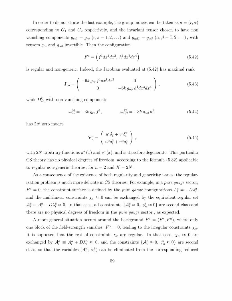
In order to demonstrate the last example, the group indices can be taken as a = (r, α)
corresponding to G1 and G2 respectively, and the invariant tensor chosen to have non
vanishing components grs1 = grs (r, s = 1, 2, . . . ) and gαβ1 = gαβ (α, β = 1, 2, . . . ) , with
tensors grs and gαβ invertible. Then the configuration
F a =(f 1dx1dx2, h1dx3dx4
)(5.42)
is regular and non-generic. Indeed, the Jacobian evaluated at (5.42) has maximal rank
Jab =
(−6k grs f
1dx1dx2 0
0 −6k gαβ h1dx3dx4
), (5.43)
while Ωijab with non-vanishing components
Ω34rs = −3k grs f
1, Ω12αβ = −3k gαβ h
1, (5.44)
has 2N zero modes
Vai =
(urδ1
i + vrδ2i
uαδ3i + vαδ4
i
), (5.45)
with 2N arbitrary functions ua (x) and va (x), and is therefore degenerate. This particular
CS theory has no physical degrees of freedom, according to the formula (5.32) applicable
to regular non-generic theories, for n = 2 and K = 2N .
As a consequence of the existence of both regularity and genericity issues, the regular-
ization problem is much more delicate in CS theories. For example, in a pure gauge sector,
F a = 0, the constraint surface is defined by the pure gauge configurations Aai = −Dλa
i ,
and the multilinear constraints χa ≈ 0 can be exchanged by the equivalent regular set
Aai ≡ Aa
i +Dλai ≈ 0. In that case, all constraints Aa
i ≈ 0, φia ≈ 0 are second class and
there are no physical degrees of freedom in the pure gauge sector , as expected.
A more general situation occurs around the background F a = (F r, F α), where only
one block of the field-strength vanishes, F α = 0, leading to the irregular constraints χα.
It is supposed that the rest of constraints χr are regular. In that case, χα ≈ 0 are
exchanged by Aαi ≡ Aα
i + Dλαi ≈ 0, and the constraints Aα
i ≈ 0, φiα ≈ 0 are second
class, so that the variables (Aαi , π
iα) can be eliminated from the corresponding reduced
59
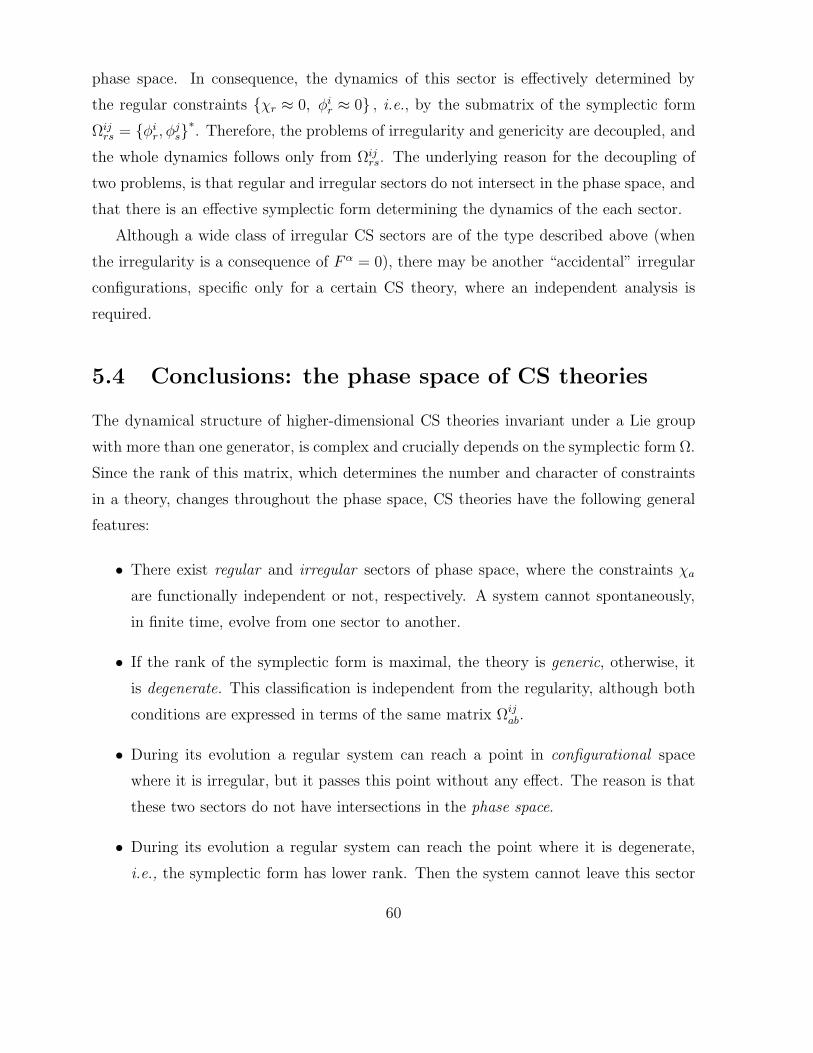
phase space. In consequence, the dynamics of this sector is effectively determined by
the regular constraints χr ≈ 0, φir ≈ 0 , i.e., by the submatrix of the symplectic form
Ωijrs = φi
r, φjs∗. Therefore, the problems of irregularity and genericity are decoupled, and
the whole dynamics follows only from Ωijrs. The underlying reason for the decoupling of
two problems, is that regular and irregular sectors do not intersect in the phase space, and
that there is an effective symplectic form determining the dynamics of the each sector.
Although a wide class of irregular CS sectors are of the type described above (when
the irregularity is a consequence of F α = 0), there may be another “accidental” irregular
configurations, specific only for a certain CS theory, where an independent analysis is
required.
5.4 Conclusions: the phase space of CS theories
The dynamical structure of higher-dimensional CS theories invariant under a Lie group
with more than one generator, is complex and crucially depends on the symplectic form Ω.
Since the rank of this matrix, which determines the number and character of constraints
in a theory, changes throughout the phase space, CS theories have the following general
features:
• There exist regular and irregular sectors of phase space, where the constraints χa
are functionally independent or not, respectively. A system cannot spontaneously,
in finite time, evolve from one sector to another.
• If the rank of the symplectic form is maximal, the theory is generic, otherwise, it
is degenerate. This classification is independent from the regularity, although both
conditions are expressed in terms of the same matrix Ωijab.
• During its evolution a regular system can reach a point in configurational space
where it is irregular, but it passes this point without any effect. The reason is that
these two sectors do not have intersections in the phase space.
• During its evolution a regular system can reach the point where it is degenerate,
i.e., the symplectic form has lower rank. Then the system cannot leave this sector
60
of lower rank since it gains additional local symmetry and looses physical degrees
of freedom there.
• In Chern-Simons theories, it is not possible to separate first from second class con-
straints explicitly, for all configurations.
The features mentioned above make the dynamics of CS theories more complicated
and with rich structure.
61
Chapter 6
AdS-Chern-Simons supergravity
It is known that gravity in 2+1 dimensions, described by the Einstein-Hilbert action with
or without cosmological constant, is exactly soluble and quantizable [9]. This is possible
because it has no local degrees of freedom, and because its action is a CS form and can
be seen as a gauge theory for the (A)dS or Poincare groups. This is an insight that
motivates the study of similar theories, represented by CS forms, in all odd dimensions
[45, 48, 50, 51] (see Appendix E). In these theories, gravity becomes a truly gauge
theory, where the vielbein (ea) and the spin-connection (ωab) are components of the same
connection field A, for the (A)dS or Poincare algebra. In higher dimensions (D ≥ 5),
the CS actions are not equivalent to the Einstein-Hilbert actions, as they contain terms
nonlinear in curvature, and torsion is a dynamical field [53].
In this chapter, CS supergravities based on the supersymmetric extensions of the AdS
group, are studied. These theories contain, apart from the gravitational fields (e, ω) and
the gravitini (ψ), a number of the additional bosonic gauge fields. The supersymmetry
algebra closes off shell, without the need to introduce auxiliary fields. The number of
boson and fermion components are not equal [56].
The simplest higher-dimensional CS supergravity with propagating degrees of freedom
occurs in five dimensions. An additional simplification is that the Lagrangian of the five-
dimensional theory does not contain torsion explicitly in the purely gravitational sector,
which is just a polynomial in the curvature and vielbein.
62
6.1 D = 5 supergravity
a) Algebra
Five-dimensional AdS -Chern-Simons supergravity is based on the supersymmetric exten-
sion of the AdS group, SU(2, 2 |N ). The superalgebra su(2, 2 |N ) is generated by the
following anti-Hermitean generators [58]:
so(2, 4) : JAB , (A,B = 0, . . . , 5) , (15 generators) ,
su(N) : TΛ , (Λ = 1, . . . , N2 − 1) , (N2 − 1) ,
SUSY : Qαr , Qr
α , (α = 1, . . . , 4; r = 1, . . . , N) , (8N) ,
u(1) : G1 , (1) ,
(6.1)
where ηAB = diag (−,+,+,+,+,−) . Lorentz rotations and AdS translations are gen-
erated by Jab and Ja ≡ Ja5 (a, b = 0, . . . , 4) respectively, and supersymmetry (SUSY)
generators transform as Dirac spinors in a vector representation of SU(N). The dimension
of this superalgebra is
N (SU(2, 2 |N )) = N2 + 8N + 15 . (6.2)
b) Field content
The fundamental field is the Lie-algebra-valued connection 1-form, A = AMGM , with
components
A =1
`eaJa +
1
2ωabJab + aΛTΛ +
(ψrQr − Qrψr
)+ φG1 . (6.3)
Apart from the purely gravitational part(
1`ea, ωab
), where ` is the AdS radius, this theory
contains a fermionic sector(ψα
r , ψrα
)(gravitini), and bosonic fields aΛ and φ demanded
by supersymmetry. The components of the field-strength F = dA + A2 = FMGM along
the bosonic generators are
F a5 = 1`T a + 1
2ψrΓaψr ,
F ab = Rab + 1`2eaeb − 1
2ψrΓabψr ,
FΛ = FΛ + ψs(τΛ)r
sψr ,
F φ = dφ− iψrψr ,
(6.4)
63
where N × N matrices τΛ are generators of su(N), and a ≡ aΛτΛ and F = da + a2 are
the corresponding field and its field-strength, dφ is the u(1) field-strength and the torsion
(T a) and curvature (Rab) two-forms are given in Appendix E. The component of the
field-strength along the fermionic generator(−QrFr term
), is
Fr = Dψr , (6.5)
where the super covariant derivative of a p-form X is DX = X + [A,X] (see Appendix
G). In particular, for the spinor ψr, it is
Dψr = (∇+ e/)ψr − asrψs + i
(1
4− 1
N
)φψr , (6.6)
where ∇ψr = (d+ ω/)ψr is the Lorentz covariant derivative, with ω/ ≡ 14ωabΓab and e/ ≡
12`eaΓa.
c) Action
The CS Lagrangian, defined by (5.1), in five dimensions becomes
dLCS = ik⟨F3⟩
= ik gMNK FMFNFK , (6.7)
where 〈. . .〉 stands for a symmetrized invariant supertrace (symmetric in bosonic and
antisymmetric in fermionic indices) which is explicitly given in Appendix F.1 The constant
k is dimensionless and real, and antisymmetric wedge product acts between the forms.
The CS action can be explicitly written as
ICS [A] =
∫M
LCS(A) = ik
∫M
⟨A (dA)2 +
3
2A3dA +
3
5A5
⟩+B [A] , (6.8)
where B [A] is a boundary term which must be added so that the action is stationary on
the classical orbits. In components, the CS supergravity action takes the form originally
obtained by Chamseddine [48],
LCS = Lg (ω, e) + LSU(N) (a) + LU(1) (ω, e, φ) + Lf (ω, e, a, φ, ψ) , (6.9)
1The symmetrized supertrace 〈 〉 ≡ 〈 , , 〉 has three Lie-algebra-valued entries. For example,⟨A3dA
⟩≡⟨A2,A, dA
⟩=⟨A,A2, dA
⟩.
64
where
Lg = k8εabcde
(1`RabRcdee + 2
3`3Rabecedee + 1
5`5eaebecedee
),
LSU(N) = −ikTrN
(aF2 − 1
2a3F + 1
10a5),
LU(1) = k(
142 − 1
N2
)φ (dφ)2 + 3k
4`2
(T aTa − `2
2RabRab −Rabeaeb
)φ+ 3k
NFΛFΛφ ,
Lf = −3ik4ψr[
1`T aΓa + 1
2
(Rab + eaeb
)Γab + 2i
(1N
+ 14
)dφ− ψsψs
]Dψr
−3ik2ψr(F s
r − 12ψsψr
)Dψs + c.c. ,
(6.10)
and F sr = FΛ (τΛ)s
r . On the basis of the form of Dψr given by (6.6), one can see that
the fermions carry a U(1) charge q = 14− 1
N. The pure gravitational Lagrangian Lg
contains the standard Einstein-Hilbert Lagrangian with negative cosmological constant,
plus an additional term quadratic in curvature which is a dimensional continuation of the
Gauss-Bonnet density from four to five dimensions.
From the Lagrangian LU(1) and the relation (6.6) it can be seen that the case N = 4 is
exceptional since the dynamics of φ changes (it looses the cubic term in the Lagrangian)
and fermions become neutral (q = 0). It is shown in the Appendix F that for N = 4, the
U(1) generator becomes a central extension.
d) Local symmetries
As all CS theories, the AdS -CS supergravity action is invariant under diffeomorphisms,
δxµ = ξµ (x), δξA = −£ξA , and infinitesimal gauge transformations, δλA = −Dλ(see the Section 5.1). In particular, under local supersymmetry transformations with
parameter εαr (x) , from λ = εrQr − Qrεr one obtains
δεea = −1
2
(ψrΓaεr − εrΓaψr
), δεψ
rα = −Dεrα ,
δεωab = 1
4
(ψrΓabεr − εrΓabψr
), δεψ
αr = −Dεαr ,
δεaΛ = ψr
(τΛ)s
rεs − ε
(τΛ)s
rψs , δεφ = −i
(ψrεr − εψr
).
(6.11)
Unlike standard supergravities, here the supersymmetry algebra closes off shell by con-
struction, without requiring auxiliary fields [56].
65
The CS action is not invariant under large gauge transformations
Ag = g (A + d) g−1 , g ∈ SU (2, 2 |N ) , (6.12)
where g = eλ. Using the fact that the field-strength transforms homogenously, Fg =
gFg−1, leading to dLgCS = dLCS, one obtains that the Lagrangian changes as Lg
CS = LCS+ω,
where ω is a closed form (dω = 0) which is not exact for nontrivial topology.
e) Field equations
Varying (6.8) with respect to the connection, yields
δICS = 3ik
∫M
⟨F2 δA
⟩, (6.13)
provided δB and the boundary conditions are chosen so that the boundary term in δICS
vanishes. Then the action has an extremum if the equations of motion are satisfied,
⟨GMF2
⟩= gMNKF
NFK = 0 . (6.14)
One solution of these equations is a connection which is locally flat, a pure gauge field,
A = gdg−1. The theory with configurations in the sector around a pure gauge field has
no propagating degrees of freedom and the entire dynamics is contained in the nontrivial
topology, but in that case the theory is irregular. In general, there are physical degrees
of freedom in the bulk, as well as at the boundary.
The asymptotic dynamics is sensitive to the choice of boundary conditions and the
topology of ∂M. The boundary conditions must be chosen so that δB can be integrated
to get B, or, if B = 0, so that δICS does not contain additional boundary terms in
(6.13). Here it is supposed that the adequate boundary conditions exist, and they will be
discussed later, in connection with the conserved charges.
6.2 Conserved charges
In Chapter 5, the Hamiltonian dynamics of CS theories in D ≥ 5 was analyzed. It
was shown that, in regular sectors of phase space, gauge invariance is expressed by the
66
presence of first class constraints GM which generate gauge transformations. There is
also diffeomorphism invariance in these theories. Spatial diffeomorphisms are generated
by first class constraints Hi, while time-like diffeomorphisms are not independent, but
realized as on-shell symmetries. Generic sectors of these theories do not have additional
independent local symmetries. The symplectic form, which defines the kinetic term in CS
theories, was also discussed. It was emphasized that it can change its rank throughout
configuration space. Depending on the rank of the symplectic form, which in general
depends on the background, CS theories can be either regular or irregular, generic or
degenerate.
The study of the boundary dynamics has been intentionally left out of the analysis. In
2+1 dimensions, where there are no locally propagating degrees of freedom, the boundary
dynamics is purely topological. In higher dimensions, besides purely topological degrees
of freedom, there also exist local ones. In this chapter, the boundary dynamics is analyzed
(see [55] for a review of the bosonic case). From now on, only regular and generic CS
theories are considered, and they in general have local degrees of freedom.
In the Hamiltonian formalism it is assumed that space-time is M ' R × σ, where σ
is an Euclidean manifold. The PB of the canonical fields(AM
i , πiM
)on the phase space Γ
is given by
πi
M , ANj
= −δi
jδNM δ = − (−)εM
AN
j , πiM
, (6.15)
where δ denotes the Dirac’s δ-function at the spatial section, AM0 is a Lagrange multiplier,
and the number εM = 0, 1 (mod 2) is the Grassmann parity of AMµ and πµ
M (see Appendix
G for the conventions). The Hamiltonian for the action (6.8) is given by
HT =
∫d4x
(AM
0 GM + uMi φ
iM
), (6.16)
where boundary terms have been neglected for the moment. The constraints are given by
φiM = πi
M − LiM ≈ 0 ,
GM = −χM +DiφiM ≈ 0 , (6.17)
67
where the covariant derivative acts on φiM as Diφ
iM = ∂iφ
iM +f K
MN AKi φ
iM and, for D = 5,
LiM = ik εijkl
(gMNK F
NjkA
Kl −
1
4gMNL f
LKS AN
j AKk A
Sl
),
χM = −3ik
4εijklgMNK FN
ij FKkl ≈ 0 . (6.18)
The symplectic form defining the kinetic term in the action is a function on phase space
ΩijMN = −3ik εijklgMNK FK
kl , (6.19)
whose rank can vary throughout Γ. In the regular and generic sectors, the action does
not have other independent symmetries apart from spatial diffeomorphisms and gauge
transformations, and the constraints satisfy the Poisson brackets algebra
GM ,GN = f KMN GK δ ,
GM , φiN
= f K
MN φiK δ , (6.20)
φiM , φ
jN
= Ωij
MN δ ,
where GM are first class constraints (generators of gauge transformations), while among
φ’s there are four first class constraints (generators of spatial diffeomorphisms) and the
rest are second class constraints. The number of locally propagating degrees of freedom
in this theory, according to (5.23), is
f5 (N) = N2 + 8N + 13 . (6.21)
Regular generic background. In the following, a class of backgrounds (solutions
of the constraints) is chosen so that they provide a regular and generic theory. They also
allow separating first and second class constraints among φ’s, which is in general a difficult
task. However, in the case of N = 4, the invariant tensor takes the same form as invariant
tensor of g ⊗ u (1). Explicitly, the supersymmetric algebra su(2, 2 |4) is generated by the
u(1) generator G1 and the psu(2, 2 |4) generators GM ′ =(JAB,TΛ,Q
αr , Q
rα
), so that the
invariant tensor gMNK , decomposed as GM → (GM ′ ,G1) , takes the simpler form (see
Appendix F):
gMNK →gM ′N ′K ′ , gM ′N ′1 = − i
4γM ′N ′ , gM ′11 = 0 , g111 = 0
. (6.22)
Here γM ′N ′ is the invertible Killing metric of PSU(2, 2 |4).
68
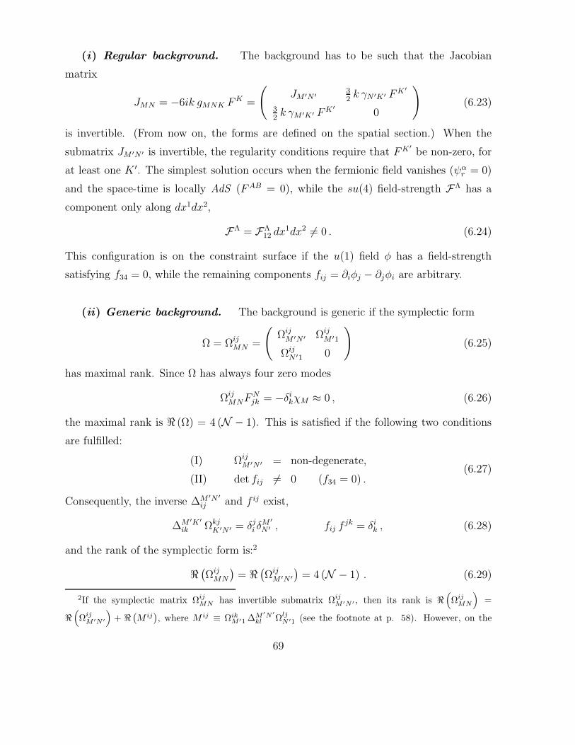
(i) Regular background. The background has to be such that the Jacobian
matrix
JMN = −6ik gMNK FK =
(JM ′N ′ 3
2k γN ′K ′ FK ′
32k γM ′K ′ FK ′
0
)(6.23)
is invertible. (From now on, the forms are defined on the spatial section.) When the
submatrix JM ′N ′ is invertible, the regularity conditions require that FK ′be non-zero, for
at least one K ′. The simplest solution occurs when the fermionic field vanishes (ψαr = 0)
and the space-time is locally AdS (FAB = 0), while the su(4) field-strength FΛ has a
component only along dx1dx2,
FΛ = FΛ12 dx
1dx2 6= 0 . (6.24)
This configuration is on the constraint surface if the u(1) field φ has a field-strength
satisfying f34 = 0, while the remaining components fij = ∂iφj − ∂jφi are arbitrary.
(ii) Generic background. The background is generic if the symplectic form
Ω = ΩijMN =
(Ωij
M ′N ′ ΩijM ′1
ΩijN ′1 0
)(6.25)
has maximal rank. Since Ω has always four zero modes
ΩijMNF
Njk = −δi
kχM ≈ 0 , (6.26)
the maximal rank is < (Ω) = 4 (N − 1). This is satisfied if the following two conditions
are fulfilled:
(I) ΩijM ′N ′ = non-degenerate,
(II) det fij 6= 0 (f34 = 0) .(6.27)
Consequently, the inverse ∆M ′N ′ij and f ij exist,
∆M ′K ′ik Ωkj
K ′N ′ = δji δ
M ′N ′ , fij f
jk = δik , (6.28)
and the rank of the symplectic form is:2
<(Ωij
MN
)= <
(Ωij
M ′N ′)
= 4 (N − 1) . (6.29)
2If the symplectic matrix ΩijMN has invertible submatrix Ωij
M ′N ′ , then its rank is <(Ωij
MN
)=
<(Ωij
M ′N ′
)+ <
(M ij
), where M ij ≡ Ωik
M ′1 ∆M ′N ′kl Ωlj
N ′1 (see the footnote at p. 58). However, on the
69
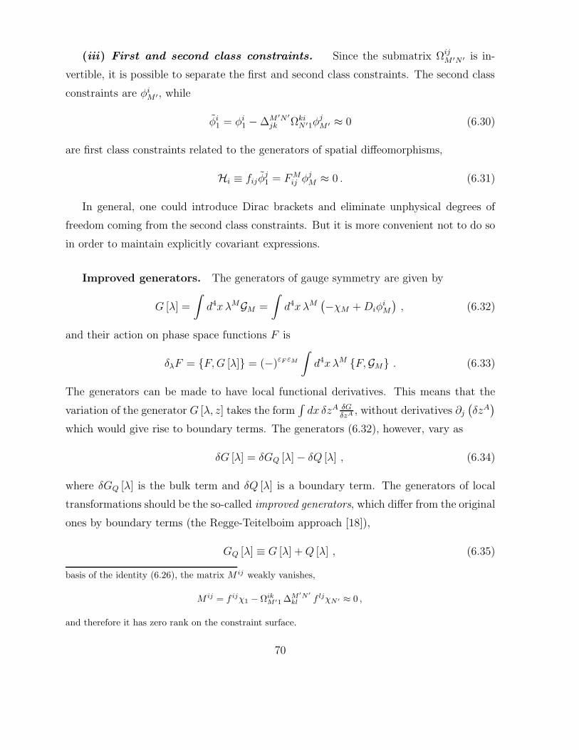
(iii) First and second class constraints. Since the submatrix ΩijM ′N ′ is in-
vertible, it is possible to separate the first and second class constraints. The second class
constraints are φiM ′, while
φi1 = φi
1 −∆M ′N ′jk Ωki
N ′1φjM ′ ≈ 0 (6.30)
are first class constraints related to the generators of spatial diffeomorphisms,
Hi ≡ fijφj1 = FM
ij φjM ≈ 0 . (6.31)
In general, one could introduce Dirac brackets and eliminate unphysical degrees of
freedom coming from the second class constraints. But it is more convenient not to do so
in order to maintain explicitly covariant expressions.
Improved generators. The generators of gauge symmetry are given by
G [λ] =
∫d4xλMGM =
∫d4xλM
(−χM +Diφ
iM
), (6.32)
and their action on phase space functions F is
δλF = F,G [λ] = (−)εF εM
∫d4xλM F,GM . (6.33)
The generators can be made to have local functional derivatives. This means that the
variation of the generator G [λ, z] takes the form∫dx δzA δG
δzA , without derivatives ∂j
(δzA)
which would give rise to boundary terms. The generators (6.32), however, vary as
δG [λ] = δGQ [λ]− δQ [λ] , (6.34)
where δGQ [λ] is the bulk term and δQ [λ] is a boundary term. The generators of local
transformations should be the so-called improved generators, which differ from the original
ones by boundary terms (the Regge-Teitelboim approach [18]),
GQ [λ] ≡ G [λ] +Q [λ] , (6.35)
basis of the identity (6.26), the matrix M ij weakly vanishes,
M ij = f ijχ1 − ΩikM ′1 ∆M ′N ′
kl f ljχN ′ ≈ 0 ,
and therefore it has zero rank on the constraint surface.
70
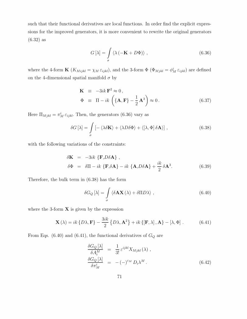
such that their functional derivatives are local functions. In order find the explicit expres-
sions for the improved generators, it is more convenient to rewrite the original generators
(6.32) as
G [λ] =
∫σ
〈λ (−K +DΦ)〉 , (6.36)
where the 4-form K (KMijkl = χM εijkl), and the 3-form Φ (ΦMjkl = φiM εijkl) are defined
on the 4-dimensional spatial manifold σ by
K ≡ −3ik F2 ≈ 0 ,
Φ ≡ Π− ik(A,F − 1
2A3
)≈ 0 . (6.37)
Here ΠMjkl = πiM εijkl. Then, the generators (6.36) vary as
δG [λ] =
∫σ
[−〈λδK〉+ 〈λDδΦ〉+ 〈[λ,Φ] δA〉] , (6.38)
with the following variations of the constraints:
δK = −3ik F,DδA ,
δΦ = δΠ− ik F,δA − ik A,DδA+ik
2δA3. (6.39)
Therefore, the bulk term in (6.38) has the form
δGQ [λ] =
∫σ
〈δAX (λ) + δΠDλ〉 , (6.40)
where the 3-form X is given by the expression
X (λ) = ik Dλ,F − 3ik
2
Dλ,A2
+ ik [F, λ] ,A − [λ,Φ] . (6.41)
From Eqs. (6.40) and (6.41), the functional derivatives of GQ are
δGQ [λ]
δAMi
=1
3!εijklXMjkl (λ) ,
δGQ [λ]
δπiM
= − (−)εM DiλM . (6.42)
71
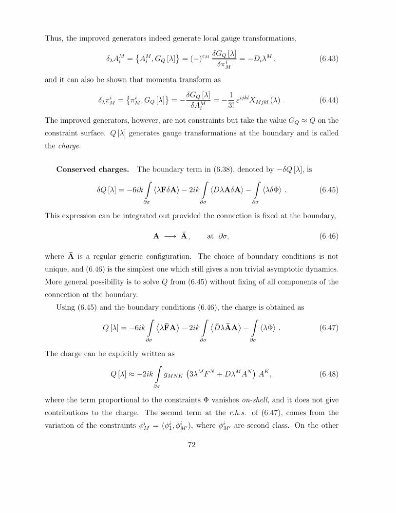
Thus, the improved generators indeed generate local gauge transformations,
δλAMi =
AM
i , GQ [λ]
= (−)εMδGQ [λ]
δπiM
= −DiλM , (6.43)
and it can also be shown that momenta transform as
δλπiM =
πi
M , GQ [λ]
= −δGQ [λ]
δAMi
= − 1
3!εijklXMjkl (λ) . (6.44)
The improved generators, however, are not constraints but take the value GQ ≈ Q on the
constraint surface. Q [λ] generates gauge transformations at the boundary and is called
the charge.
Conserved charges. The boundary term in (6.38), denoted by −δQ [λ], is
δQ [λ] = −6ik
∫∂σ
〈λFδA〉 − 2ik
∫∂σ
〈DλAδA〉 −∫∂σ
〈λδΦ〉 . (6.45)
This expression can be integrated out provided the connection is fixed at the boundary,
A −→ A , at ∂σ, (6.46)
where A is a regular generic configuration. The choice of boundary conditions is not
unique, and (6.46) is the simplest one which still gives a non trivial asymptotic dynamics.
More general possibility is to solve Q from (6.45) without fixing of all components of the
connection at the boundary.
Using (6.45) and the boundary conditions (6.46), the charge is obtained as
Q [λ] = −6ik
∫∂σ
⟨λFA
⟩− 2ik
∫∂σ
⟨DλAA
⟩−∫∂σ
〈λΦ〉 . (6.47)
The charge can be explicitly written as
Q [λ] ≈ −2ik
∫∂σ
gMNK
(3λM FN + DλM AN
)AK , (6.48)
where the term proportional to the constraints Φ vanishes on-shell, and it does not give
contributions to the charge. The second term at the r.h.s. of (6.47), comes from the
variation of the constraints φiM = (φi
1, φiM ′), where φi
M ′ are second class. On the other
72
hand, one should not expect to have a contribution of the second class constraints, which
naturally do not appear in the gauge generator (6.36) on the reduced phase space, where
φiM ′ = 0, what can be explicitly provided by introducing the appropriate Dirac brack-
ets. Both approaches should be equivalent, because the second class constraints do not
generate gauge transformations, and there are no conserved charges associated to them.
One can see that the term⟨Dα, A,A
⟩vanishes for the local PSU (2, 2 |4) parameter
α ≡ αM ′GM ′ , once the asymptotic conditions are used. Evaluated at the background
(A = A), this term is indeed zero, due to the identity gM ′NK AN AK ≡ 0. The fields
asymptotically tend to the background, so that the connection behaves as A ∼ A + ∆A,
while the local parameter is α ∼ α+∆α, where α is a covariantly constant vector (Dα = 0)
which describes symmetries of the vacuum at the boundary. Then the term
⟨Dα, A,A
⟩∼⟨D∆α, A,∆A
⟩, (6.49)
gives a contribution of second order, since ∆A and ∆α are subleading compared to A
and α, in the limit in which the boundary is taken to infinity.
Charge algebra. The PB algebra of improved gauge generators can be found di-
rectly from the definition of the functional derivatives (6.42), and it has the form
GQ [λ] , GQ [η] =
∫σ
〈X (λ)Dη −X (η)Dλ〉 , (6.50)
where the expression for X is given by (6.41). This algebra closes, and it has the general
form
GQ [λ] , GQ [η] = GQ [[λ, η]] + C [λ, η] , (6.51)
where [λ, η]M = −f MKN λNηK , and C [λ, η] is a boundary term. Thus, the classical algebra
acquires a central extension C, called the central charge, which emerges as a consequence
of working with the improved generators. In order to calculate C, rather than starting
from (6.50), it is more convenient to find it from the gauge transformation of the charge
Q,
δηQ [λ] = Q [λ] , Q [η] = Q [[λ, η]] + C [λ, η] . (6.52)
73
On the basis of the Brown-Henneaux theorem [112], the central extension obtained from
the gauge transformation of the charge, Eq. (6.52), is the same as the central charge
in the algebra of improved generators, Eq. (6.51), evaluated on the background. This
follows from the fact that the charge algebra (6.52) is valid only on the reduced phase
space, after gauge fixing of all first class constraints GM , so that the original generators
G [λ] are all strongly zero.
The central charge can be evaluated as follows. In the class of generic regular configura-
tions A given by (6.24) and (6.27), the vacuum Av is the one for which the charges vanish,
Q [λ] ≡ Q [λ]Av= 0. Then, the central charges are obtained as C [λ, η] = δηQ [λ]Av
. This
will be calculated in the next section.
6.3 Killing spinors and BPS states
In supergravity theories, the anticommutation relation are of the formQ,Q† ∼ P +
J + · · · , giving that the sum of the total charges is bounded from below, since it is
proportional to∑(
QQ† +QQ†) ≥ 0 (Bogomol’nyi bound [36]). In standard supergravity
theories it leads to the positivity of energy [37, 38, 39]. When the bound is saturated,
the corresponding states, the so-called BPS states, have some unbroken supersymmetries.
Therefore, the existence of BPS states is important for the stability of the theory. In what
follows, a BPS state will be constructed which is also regular and generic.
For the bosonic BPS states ψαr = 0, and the supersymmetry transformations δεψ
αr =
−Dεαr leave this condition invariant if the local fermionic parameter satisfies
Dεαr = 0 . (6.53)
This is the Killing equation for the spinor εαr , and its solutions are Killing spinors.
Assuming a generic regular configuration, conditions (6.24) and (6.27) are satisfied if:
ψr = 0 , FΛ = FΛ12 drdϕ
2 6= 0 ,
FAB = 0 , det fij 6= 0 , f34 = 0 .(6.54)
The local coordinates onM are chosen as xµ = (t, r, xn), where xn (n = 2, 3, 4) parametrize
the boundary ∂σ, placed at the infinity of the radial coordinate r.
74
Locally AdS space-time. The AdS space-time (FAB = 0) can be described by the
metric
ds2AdS = `2
(dr2 + e2rηnm dx
ndxm), (6.55)
where xn = (t, xn) and ηnm = diag (−,+,+,+,+). The vielbein (ea) and the spin
connection (ωab) are given by
e1 = `dr , ωn1 = 1`en = erdxn ,
en = `erdxn , ωnm = 0 .(6.56)
It is easy to check that this space-time is indeed torsionless (T a = 0) and with constant
negative curvature (Rab = − 1`2eaeb). Then the AdS connection is
W =1
4WABΓAB =
1
2`
[e1Γ1 + enΓn (1 + Γ1)
]. (6.57)
The Killing spinors εα for the metric (6.55), which are solutions of
(d+ W) ε = 0 , (6.58)
and they have the form [135]
ε = e−r2
Γ1 [1− xnΓn (1 + Γ1)] ε0 , (6.59)
where ε0 is a constant spinor. The derivation of (6.59) is given in the Appendix H.
Changing the topology of ∂σ by the identification of the coordinates xn gives a locally AdS
space-time, and it eliminates the xn-dependence of ε, which therefore must be (anti)chiral
under Γ1. Some examples of Killing spinors in the locally AdS space-time are given in
[136].
Consistency of the Killing equation. The Killing equation (6.53) for the su(4)
spinor εαr can be written in components as
[δsr (d+ W)− as
r] εs = 0 , (6.60)
where WAB =(
1`ea, ωab
)is the AdS connection, a is the su(4) connection, and (for
N = 4) the u(1) field is decoupled and it does not appear in the covariant derivative. The
75
consistency of this equation requires DDε = [F, ε] = 0, or in components,(1
4δsr F
ABΓAB − F sr
)εs = 0 . (6.61)
For the configurations (6.54), this equation reduces to
F sr εs = 0 . (6.62)
This equation has nonvanishing solution provided the matrix F sr has zero eigenvalues
and εr are its zero modes. In order to have a nontrivial su(4) curvature, FΛ must be
nonvanishing for more than one value of the index Λ, so that the contributions of all
components cancel. Using the local isomorphism su(4) ' so(6), it is more convenient to
represent the su(4) curvature as F sr = 1
2F IJ (τIJ)s
r, where
τIJ =1
2ΓIJ , (I, J = 1, . . . , 6) (6.63)
are the so(6) generators, ΓIJ = 12
[ΓI , ΓJ
]and ΓI are the Euclidean Γ-matrices. Fur-
thermore, the commuting matrices τ12 and τ34 generate the u(1) ⊗ u(1) subalgebra of
so(6). Since (τ12)2 = (τ34)
2 = −14, the eigenvalues of τ12 and τ34 are ± i
2. Considering the
“twisted” configuration, i.e., assuming
(τ12)sr εs =
i
2εr ,
(τ34)sr εs = − i
2εr , (6.64)
and that the only u(1) curvature components are F12 = da12 and F34 = da34, then Eq.
(6.62) becomes i2
(F12 − F34) εr = 0 , whose solution is
F12 = F34. (6.65)
In terms of the connection, this implies
a12 = a34 + dη , (6.66)
where η (r, xn) is an arbitrary function. Since F1212 (r, x2) can only depend on two coordi-
nates by virtue of the Bianchi identity, the simplest solution reads
a12 (x2) = ρ (x2) dr ,
F12 (x2) = −ρ′ (x2) drdx2 .(6.67)
76
The Killing spinors. Since asr εs = i
2dη εr, the su(2, 2 |4) Killing equation (6.60)
reduces to (d+ W − i
2dη
)εs = 0 , (6.68)
where W is given by (6.57). The spinor εs can be factorized as
εαs = us εα , (6.69)
where the spinor εα is the AdS Killing spinor (6.59), while the su(4) vector us is a solution
of the equation (d− i
2dη
)us = 0 , (6.70)
and it has the form us = ei2
ηu0s. Therefore, The spinor εs is
εs = ei2
ηe−r2
Γ1 [1− xnΓn (1 + Γ1)] ε0s , (6.71)
where the constant spinor εα0s satisfies the conditions (6.64)
(τ12)sr ε0s =
i
2ε0r , (τ34)
sr ε0s = − i
2ε0r . (6.72)
The norm ‖ε‖2 = εε is constant and positive,
‖ε‖2 = ‖ε0‖2 > 0 , (6.73)
where εrα = εr†β (Γ0)βα (see Appendix H).
Therefore, the existence of configurations with some unbroken supersymmetries, which
saturate the Bogomol’nyi bound, is important for the stability of the theory. Among them,
there is the ground state Av.
The central charge. A pending issue is to find the explicit expression of the central
charge, C, for the charge algebra (6.52). This can be done for the configurations that
asymptotically tend to the background solution which is a BPS state. Since FM ′= 0 at
the boundary, the only nonvanishing field-strength is f , and the charge (6.47) becomes
Q [λ] = −3k
4
∫∂σ
f(λIJ a
IJ + λABWAB). (6.74)
77
The goal is to find the vacuum, for which all charges vanish, Q [λ] = 0. The su(4) fields
are given by (6.66) and (6.67), so that the first term in the expression for the charge (6.74)
is proportional to the pure gauge dη. Therefore, for the vacuum state, η can be chosen so
that dη = 0. On the basis of (6.56), the second term in the charge (6.74) vanishes if the
AdS parameters λn5, λn1 obey the asymptotic conditions:
εnmkfnm (λk5 + λk1) er → 0 , (r →∞) . (6.75)
Supposing that all conditions are fulfilled and Q = 0, the charge Q [λ] in (6.47) is
found to change under the gauge transformations δηA = −Dη, as
C [λ, η] = 2ik
∫∂σ
⟨(3λF+DλA
)Dη⟩. (6.76)
Finally, after substitution of the BPS background, the charge becomes
C [λ, η] = k
∫∂σ
f ηM ′dλM ′ . (6.77)
The algebra (6.51), with the central charge (6.77), is a supersymmetric extension of
the WZW4 algebra [46, 47, 54, 57]. This algebra has a nontrivial central extension for
PSU(2, 2 |4), which depends on the 2-form f . In the Ref. [54], the WZW4 algebra de-
scribing the asymptotic symmetries of a CS theory based on g⊗u(1) algebra was studied.
The background chosen there was irregular, and it was not possible to define the u(1)
charge, so that the WZW4 algebra was associated only to the subalgebra g. In the case
of the superalgebra (6.51), all generators are well defined because the chosen background
is regular and generic. In contrast, the super WZW4 algebra obtained here is associated
to the full gauge group SU(2, 2 |4).
6.4 Conclusions
In this chapter, CS supergravities based on the supersymmetric extension of the AdS 5
algebra, su(2, 2 |N ) were analyzed. This supergravity theories contain the gravitational
fields, 2N gravitini, su(N) bosonic fields, and u(1) field. The action, apart from the
Einsten-Hilbert term, contains terms nonlinear in curvature and is torsionless. The syper-
symmetry algebra closes off-shell, without bringing in the auxiliary fields.
78
In the case of N = 4, the invariant tensor of su(2, 2 |4) algebra has the same form as
the invariant tensor of g⊗u(1). The theory has rich local dynamics, with 61 locally prop-
agating degrees of freedom in the regular generic sector, as well as nontrivial asymptotic
dynamics.
The asymptotic dynamics depends on the choice of boundary conditions and is deter-
mined by the subset of the gauge transformations which preserve these conditions at the
boundary. A result of this analysis was to show that adequate boundary conditions exist,
and to find the corresponding symmetries and the charges at the boundary.
The following results are obtained:
• A class of backgrounds is found, which provide a regular and generic theory. They
are locally AdS space-times with bosonic su(4) and u(1) matter. It is impossible
to have a regular and generic AdS space-time without both types of bosonic matter
fields. On the other hand, if AdS space-time is not required, then the su(4) field-
strength can vanish (pure-gauge).
• Around the chosen backgrounds, the first and second class constraints are explicitly
separated. This, in general, is an extremely difficult task for an arbitrary CS theory.
• The charges corresponding to the complete gauge symmetry are obtained for the
simplest choice of the asymptotic conditions A → A. This problem is not trivial
since higher-dimensional CS theories are irregular systems and there are sectors in
the phase space where it is not possible to define some generators.
• BPS states exist among the considered backgrounds, which is important for the
stability of the theory.
• The supersymmetric extension of the classical WZW4 algebra, associated to su(2, 2 |4),
is obtained. The nontrivial central extension occurs only for psu(2, 2 |4) subalgebra.
In addition to these results, work on the asymptotics of the CS supergravity is in
progress, because there are still many questions to be answered. One of them is related to
the finding of the asymptotic symmetries and the physical interpretation of the conserved
charges. For example, is the mass associated to the generator of the local time translations
79
Q [λa5]? In Ref. [113], the energy and angular momentum of the black hole embedded in
this supergravity theory were found, but the considered solution belonged to the irregular
sector. There are also other black hole solutions in the five-dimensional CS supergravity
which may be considered [114]–[117]. Then, the natural question is to analyze which
charges (or their combinations) are bounded from below by the Bogomol’nyi bound. For
example, in 3D supergravity, the black hole solution with the zero mass and zero angular
momentum is a BPS state, as well as the extreme case M = ` |J | [118].
Furthermore, for the BPS states obtained in the last section, it is straightforward to
make the mode expansion of the super WZW4 algebra, for instance when a boundary has
a topology S1× S1× S1, or S1 × S2. It is interesting to see which are the implications of
different topologies to the asymptotic symmetry.
One of the interesting questions which remains to be investigated, is whether there is
a regular and generic background (for example, when the su(4) field does not vanish at
the boundary) which leads to the super WZW4 with the u(1) central extension, as well.
It seems, in general, possible.
80
Chapter 7
List of main results and open
problems
Main results
• The action for the two-dimensional super Wess-Zumino-Witten model coupled to
supergravity is obtained by canonical methods, so that it is invariant under local
supersymmetry transformations by construction.
• Standard Dirac’s procedure for dealing with constrained systems is generalized to the
cases when the constraints are functionally dependent (irregular). These irregular
systems are classified, and regularized when possible, for classical theories with finite
number of degrees of freedom.
• Higher-dimensional Chern-Simons theories are analyzed in the context of irregular
systems, and the criterion which recognizes irregular sectors in their phase space is
presented.
• The dynamical content of AdS 5-Chern-Simons supergravity theory in five dimen-
sions, based on the group SU(2, 2 |4), is studied and, among them, a class of BPS
states is found.
• The classical super WZW4 algebra associated to su(2, 2 |4), with nontrivial central
extension, is obtained as the charge algebra for AdS 5-CS supergravity.
81
Open problems
• The method of construction of a super WZW action coupled to supergravity can be
generalized to the cases of N > 1 supersymmetry, in D = 2.
• It is not clear whether all types of irregular systems can be consistently quantized,
and how irregular sectors will present themselves after the quantization.
• The dynamic of irregular and degenerate Chern-Simons theories, in which the ir-
regular sectors intersect with the surfaces of phase space with lower rank of the
symplectic form, is not well understood.
• The pending questions in the AdS 5-Chern-Simons supergravity are the identification
of the asymptotic symmetries and conserved charges in terms of observables (the
mass, angular momentum, electric charge, etc.), as well as analysis of its boundary
dynamics for different choices of topology of the space-time.
• One of more general problems is to obtain an action for a super WZW model in
higher dimensions. It can be done, for example, solving the CS theory in D = 5
based on the supersymmetric extension of U(1) ⊗ U(1), and finding its theory at
the boundary.
82
Appendix A
Hamiltonian formalism
In this chapter, the Hamiltonian formalism for the systems with bosonic degrees of freedom
is reviewed [98, 101], [119]–[123]. A generalization of the formalism to the systems with
fermionic degrees of freedom can be found in Refs. [124]–[127], while for the reviews see
Refs. [59, 99, 102], [128]–[131].
Consider a classical system with finite number of degrees of freedom, described by the
action
I[q, q] =
∫ t1
t0
dt L(qi, qi) , (i = 1, · · · , N) , (A.1)
which depends at most on first derivatives of the local coordinates qi(t) (up to divergence
terms) and it does not depend on time explicitly. The classical dynamics is derived from
the Hamilton’s variational principle, as a stationary point of the action under variations
δq(t) with fixed endpoints δq(t0) = δq(t1) = 0.
a) Dirac-Bergman algorithm
In order to pass to the Hamiltonian formalism, momenta are defined in the usual way as
pi =δI
δqi, (i = 1, · · · , N) , (A.2)
and Hamiltonian dynamics happens on 2N -dimensional phase space
Γ = zn | n = 1, . . . , 2N , (A.3)
83
with local coordinates zn = (qi, pj). When all velocities can be solved from the equations
(A.2) in terms of canonical variables, the evolution of a system is uniquely determined from
its initial configuration by means of Hamilton equations. When all velocities qi cannot
be uniquely solved from equations (A.2) in terms of canonical variables, all momenta are
not independent. In consequence, there are primary constraints,
ϕα (z) = 0 , (α = 1, · · · , NP ) , (A.4)
which define the primary constraint surface
ΣP = z ∈ Γ | ϕα(z) = 0 (α = 1, . . . , NP ) (NP ≤ 2N) . (A.5)
Although the primary constraints vanish on ΣP , their derivatives do not, thus it is
useful to make difference between the concepts of weak and strong equalities. A function
F (z), defined and differentiable in a neighborhood of z ∈ Γ, is weakly equal to zero if it
vanishes on ΣP ,
F (z) ≈ 0 ⇐⇒ F (z)|ΣP= 0 , (A.6)
and it is strongly equal to zero if the function F and its first derivatives vanish on ΣP ,
F (z) = 0 ⇐⇒ F,∂F
∂zn
∣∣∣∣ΣP
= 0 . (A.7)
With this conventions, the primary constraints are
ϕα (z) ≈ 0 , (α = 1, · · · , NP ) . (A.8)
Primary constraints are functionally independent if the regularity conditions (RCs) [98]
are fulfilled: the constraints ϕα ≈ 0 are regular if and only if their small variations
δϕα evaluated on Σp define NP linearly independent functions of δzn.
When the RCs are satisfied, there is relation between the strong and weak equalities.
If a phase space function F is weakly equal to zero, then it is strongly equal to a linear
combination of constraints,
F ≈ 0 ⇐⇒ F = uαϕα . (A.9)
Therefore, the existence of primary constraints naturally leads to appearance of arbitrary
functions of time uα(t) in a theory.
84
Total Hamiltonian and time evolution. The canonical Hamiltonian, obtained
by Legendre transformation of the Lagrangian,
H0(q, p) = piqi − L(q, q) , (A.10)
depends only on canonical variables. Due to presence of primary constraints, canonical
variables are not independent andH0 is not unique, therefore the Legendre transformation
is not invertible. Using the relation between the weak and strong equalities (A.9), one
introduces total Hamiltonian as
H = H0 + uαϕα . (A.11)
It gives an invertible Legendre transformation, but the dynamics following from (A.11)
depends on NP arbitrary functions uα(t). Introducing a Poisson bracket (PB) on the
phase space Γ as
F,G =∂F
∂znωnm ∂G
∂zm, (A.12)
where ωnm is the antisymmetric symplectic form which determines the basic PB zn, zm =
ωnm, Hamilton equations can be written as
zn = zn, H0+ uα zn, ϕα ≈ zn, H . (A.13)
Time evolution of phase space functions F is determined by
F = F,H0+ uα F, ϕα ≈ F,H , (A.14)
and in general it is not unique for given initial conditions F (t0).
Consistency conditions. Consistency of the theory during its time evolution re-
quires that the primary constraints are preserved in time,
ϕα = ϕα, H0+ uβ ϕα, ϕβ ≈ 0 . (A.15)
These consistency conditions reduce to one of the following possibilities1:
1The systems in which the consistency conditions are not satisfied are excluded because, in such
inconsistent models, the action has no stationary points.
85
• If ϕα, ϕβ ≈ 0 and ϕα, H0 ≈ 0, then Eq. (A.15) is automatically satisfied (it
reduces to 0 ≈ 0).
• If ϕα, ϕβ ≈ 0 and ϕα, H0 6= 0, Eq. (A.15) is independent on multipliers and
gives a secondary constraint.
• If ϕα, ϕβ 6= 0, Eq. (A.15) becomes an algebraic equation in multipliers, leading
to restrictions on some of them.
Therefore, consistency conditions can give secondary constraints, the evolution of sec-
ondary constraints can give a new generation of constraints, and so on, until it stops after
finite number of generations (because the dimension of Γ is finite). This procedure results
with the complete set of constraints
φr(z) ≈ 0 , (r = 1, . . . , R) , (A.16)
and a number of determined multipliers u.
A system is regular if all constraints satisfy the RCs; otherwise, the system is irregular.
Here only regular systems are considered. Then the conditions (A.16) define (2n − R)-
dimensional constraint surface
Σ = z ∈ Γ | φr(z) = 0 (r = 1, . . . , R) (R ≤ 2N) , (A.17)
and weak and strong equalities are defined with respect to Σ. Dirac-Bergman procedure
guarantees that the system remains on the constraint surface during its evolution.
First and second class functions. A function F (z) is said to be first class if it
has a PB with all constraints weakly vanished,
F, φr ≈ 0 , (r = 1, . . . , R) . (A.18)
A function that is not first class, is called second class. As a consequence of Dirac-Bergman
procedure, the total Hamiltonian H is a first class function.
In particular, the constraints (A.16) can be divided into first and second class con-
straints. While distinction of primary and secondary constraints is of minor importance
86
in the final form of the Hamiltonian theory, the classification on first and second class
constraints has important dynamical consequences.
First class constraints commute with all other constraints, φ I class, φr ≈ 0, thus
their consistency conditions give no restrictions on multipliers. Consequently, the final
dynamics is not uniquely determined by initial conditions, and unphysical difference is
related to the existence of local symmetries in a theory.
Second class constraints have φ II class, φr 6= 0, and their consistency conditions solve
a number multipliers. The total Hamiltonian with solved multipliers is
H ′ = H ′0 + vaφa , (A.19)
where φa are primary first class constraints. Both Hamiltonians H ′ and H ′0 are first class
functions.
b) Dirac brackets
Consider a set of all second class constraints,
θm(z) ≈ 0 , (m = 1, . . . , N2) , (A.20)
where the corresponding PB matrix, or Dirac matrix, is non-degenerate,
θm, θk = ∆mk , (A.21)
with an inverse ∆mk(∆mn∆nk = δk
m
). The rank of Dirac matrix is even, as it is antisym-
metric, thus there are always even number of second class constraints.
The Dirac bracket (DB) of two phase space functions is defined by
F,G∗ = F,G − F, θm∆mk θk, G , (A.22)
and it has all properties of a PB: antisymmetry, bilinearity and it obeys product rule
and Jacobi identity. By construction, DB of second class constraints with any function F
vanishes,
θm, F∗ = 0 . (A.23)
87
Therefore, using DB instead of PB, the second class constraints can be exchanged by
strong equalities (set to zero before evaluating DB) on the reduced phase space Γ ⊂ Γ,
where θm = 0.
The construction of DB has iterative property : a subset of second class constraints can
be used to define a preliminary DB ∗. The next set of secondary constraints define a
new DB ∗∗, where a preliminary DB is used instead of a PB in the definition (A.22);
and so on, until all second class constraints are exhausted.
Gauge conditions. Unobservable degrees of freedom can be eliminated by imposing
gauge conditions
Ψa (z) ≈ 0 . (A.24)
The choice of functions Ψa has to be such that: (a) gauge conditions are accessible, or that
the equation Ψa (z) + δεΨa (z) = 0 has a solution in ε, and (b) this solution is unique, i.e.,
there is no a residual gauge symmetry which preserves gauge conditions (A.24). When
(a) and (b) are fulfilled, then the number of the gauge conditions is equal to the number
of first class constraints
χa (z) ≈ 0 , (a = 1, . . . , N1) , (A.25)
and the matrix
χa,Ψb = σab (A.26)
is invertible. The gauge conditions must be preserved in time and their consistency
conditions determine all multipliers. Ψa are treated as any other constraints in a theory
and, together with χa, they form a set of second class constraints. One can define DB
which treat all constraints and gauge conditions as strong equalities at reduced phase space
Γ∗, containing only physical degrees of freedom which number is given by the formula
N∗ = 2N − (2N1 +N2) . (A.27)
This formula applies only to the regular systems.
88
c) Local symmetries
Due to the presence of arbitrary multipliers va in the Hamiltonian (A.19), the evolution of
a variable F (t) cannot be uniquely determined from the given initial values F (t0). After a
short interval δt = t− t0, the difference of two F ’s, for two different choices of multipliers
va1 and va
2 , has the form
∆F (δt) = εa F, φa , (A.28)
where εa = (va2 − va
1) δt. This difference is unphysical and corresponds to a gauge trans-
formation generated by primary first class constraints φa. Two successive gauge trans-
formations of type (A.28), with parameters εa1 and εa
2, gives
(∆1∆2 −∆2∆1)F (δt) = εa1ε
b2 F, φa, φb , (A.29)
thus φa, φb, containing secondary first class constraints, also generates gauge trans-
formations. Dirac conjectured that all first class constraints are generators of gauge
symmetries, what will be discussed below.
Physical observables are quantities independent on arbitrary multipliers. These are
gauge invariant objects.
Generator of local symmetries. The Hamiltonian formalism provides an algo-
rithm to construct the generators of all gauge symmetries of the equations of motion
(A.13). If the gauge transformations have canonical form
δεzn = zn, G [ε] , (A.30)
where ε(t) is an infinitesimal local parameter, and the generator is
G [ε] = εG1 + εG0 , (A.31)
then necessary and sufficient conditions that Hamilton equations (A.13) are invariant
under (A.30) are
G1 = pfc ,
G0 + G1, H = pfc , (A.32)
G0, H = pfc ,
89
where ‘pfc’ stands for a primary first class constraint. Thus, G0 and G1 are determined
only up to primary first class constraints. This is Castellani’s method and it can be
generalized to the systems containing higher derivatives of a local parameter [101, 102].
Dirac conjecture. Dirac conjectured that all first class constraints are generators
of the gauge symmetries [98]. From Castellani’s method it can be seen that the genera-
tors contain, apart from the primary first class constraints G1, also secondary constraints
appearing in G1, H. Since any higher power of constraints can be treated as strong
equality, Castellani’s algorithm stops if one obtains G1, H = φK = 0 (K ≥ 2). There-
fore, the Dirac conjecture is replaced by the statement that all first class constraints
generate gauge symmetry, apart from those appearing in the consistency conditions as a
higher power of a constraint φ, and those following from the consistency conditions of φ
[102].
d) Extended action
The total Hamiltonian (A.11) contains only primary constraints. Because the separation
on primary and secondary constraints has no physical implications, it is natural to define
a Hamiltonian which contains all constraints in a theory, or extended Hamiltonian
HE = H0 + urφr . (A.33)
This Hamiltonian contains more dynamical variables than HT , thus the dynamics derived
from the extended Hamiltonian is not equivalent to the Lagrangian one, but the difference
is unphysical. The introduction of HE is a new feature of the Hamiltonian scheme, which
extends the Lagrangian formalism by making manifest all gauge freedom.
The action with the dynamics equivalent to that obtained from HE is a canonical
extended action
IE [q, p, u] =
t1∫t0
dt(qi pi −H0 − urφr
), (A.34)
and it can always be reduced to the original action by gauge fixing of all extra multipliers.
90
In a theory with only first class constraints, the following PB are satisfied
φr, φs = C prs φp , φr, H0 = C s
r φs , (A.35)
where C prs (z) and C s
r (z) are structure functions. Then the action IE [q, p, u] is invariant
under the following gauge transformations [99]:
δεzn = zn, εrφr , (A.36)
δεur = εr + C r
ps usεp + C r
s εs . (A.37)
91
Appendix B
Superspace notation in D = 2
Two-dimensional space-time manifold M with signature (−,+) is parametrized by the
local coordinates xµ = (τ, σ) , where µ = 0, 1.
In the tangent Minkowski space, the local coordinates xm (m = 0, 1) are exchanged by
the light-cone coordinates xa (a = +,−), defined by x± ≡ 12(x0 ± x1). In the light-cone
basis, the Minkowski metric ηmn = diag (−1, 1) , and its inverse ηmn, become
ηab =
(0 −2
−2 0
), ηab =
(0 −1
2
−12
0
), (B.1)
and therefore the raising and lowering of the tangent space indices is performed as V± =
−2V ∓. The Levi-Civita tensor εmn (ε01 = 1) in the light-cone basis takes the form
εab =
(0 −1
2
12
0
), εab =
(0 2
−2 0
). (B.2)
Representation of γ-matrices. Dirac matrices, defined in the tangent space, sat-
isfy the Clifford algebra
γm, γn = 2ηmn . (B.3)
The following representation is used:
γ0 =
(0 1
−1 0
), γ1 =
(0 1
1 0
), γ ≡ γ0γ1 =
(1 0
0 −1
), (B.4)
92
so that there is the identity Tr (γmγnγ) = 2εmn. The projective γ-matrices γ± = 12(γ0 ±
γ1) are represented as:
γ+ =
(0 1
0 0
), γ− =
(0 0
−1 0
). (B.5)
Spinors. A Majorana spinor is a Dirac spinor θα ≡(θ+
θ−
)which obeys the Ma-
jorana condition θ = CθT , with θ ≡ θ†γ0, and Cαβ is the charge conjugation matrix
(C−1γµC = −γTµ ). In the representation (B.4) and with C = γ0, the Majorana spinors
are real, θ∗α = θα. The inverse tensor (C−1)αβ ≡ Cαβ performs the raising of spinor indices
(θα = Cαβθβ), while Cαβ performs their lowering (θα = Cαβθβ). In components, it gives
θ± = ±θ∓. Spinor contraction is denoted by θξ ≡ θαξα = −θαξα.
Super covariant derivative. (1, 1) superspace is parametrized by four real coordi-
nates zA = (xa, θα), where xa are the light-cone coordinates and θα is a Majorana spinor.
The supercovariant derivative is
Dα = ∂α + i (γmθ)α ∂m , (B.6)
where ∂m ≡ ∂/∂xm and ∂α ≡ ∂/∂θα. More explicitly, the derivative (B.6) in the repre-
sentation (B.4) is
D± ≡ ∂θ∓ − iθ∓∂± , (B.7)
where Dα ≡(−D+
D−
).
Super δ-function. A generalization of the δ-function to the super δ-function is
δ±12 ≡ θ∓12 δ(x±1 − x±2 ) , (B.8)
where θ12 = θ1 − θ2. It has the following properties:∫d4z1 δ±12 = 1 , δ±21 = −δ±12 ,
F (z1) δ±12 = F (z2) δ±12 , D±1 δ±12 = −D±
2 δ±12 ,(B.9)
where d4z ≡ d2x d2θ and basic integrals for Grassman odd numbers are∫dθ = 0 and∫
dθ θ = 1.
93
Appendix C
Components of the vielbein and
metric in the light-cone basis
At each point of the curved space-time M, there is a light-cone basis of 1-forms ea ≡ea
µ dxµ. The vielbein ea
µ (a = +,−; µ = 0, 1) is expressed in terms of variables
(h−, h+, F, f) as
e±µ = eF±f e±µ , eaµ =
1
2
(−h+ 1
h− −1
). (C.1)
The inverse vielbein eµa (ea
µeµb = δb
a and eµaea
ν = δνµ) is
eµ± = e−(F±f)eµ± , eµ
a =2
h− − h+
(1 1
h− h+
). (C.2)
The related basis of tangent vectors ∂a ≡ eµa∂µ can be written as
∂± = e−(F±f)∂± , ∂± =2
h− − h+(∂0 + h∓∂1) . (C.3)
It follows from (C.1) that the components of the metric tensor gµν = ηab eaµe
bν are
gµν = e2F gµν , gµν ≡ −1
2
(−2h+h− h+ + h−
h+ + h− −2
), (C.4)
while the inverse metric gµν has components
gµν = e−2F gµν , gµν ≡ − 2
(h− − h+)2
(2 h+ + h−
h+ + h− 2h−h+
). (C.5)
94
Here√−g = e2F
√−g ≡ e2F h−−h+
2.
The Riemannian connection onM is defined by T a = 0 as
ωa = εbc eµb ∂ceaµ , (C.6)
where εmn (ε01 = 1) is the constant totally antisymmetric tensor in the Minkowski space
or, in light-cone basis, ε−+ = −ε+− = 12. Written in terms of variables (C.2) and (C.3),
the connection becomes
ω± = e−(F±f)[ω± ∓ ∂±(F ∓ f)
], ω± ≡ ∓
2∂1h∓
h− − h+. (C.7)
Covariant derivative in the conformally flat (light-cone) coordinates, acting on a Weyl
field with the weight n, is
Oa = ∂a +n
2ωa , (C.8)
or explicitly
O± = e(±n−1)F−(n±1)f O± e∓nF+nf , (C.9)
where Oa = ∂a + n2ωa.
95
Appendix D
Symplectic form in Chern-Simons
theories
Consider a Chern-Simons (CS) theory in D = 2n + 1 ≥ 5 dimensions described by the
action in Hamiltonian form (first order formalism)
ICS[Aai ] =
∫R×σ
LCS(A) =
t1∫t0
dt
∫σ
d2nx(Li
a Aai − Aa
0χa
), (D.1)
dLCS = k ga1···an+1 Fa1 · · ·F an+1 , (D.2)
where Aai define a space of gauge fields A and Aa
0 is Lagrange multiplier. Similarly to
the basis of 1-forms dxµ on the space-time manifoldM, one can define a basis of 1-forms
δAai (x) on the manifold of gauge fields A. The symplectic form Ω is a quadratic 2-form
defining the kinetic term in (D.1),
ICS =
∫dt Ω δAδA
=
∫dt
∫d2nx
∫d2nx′ Ωij
ab (x, x′) δAai (x) δAb
j (x′) , (D.3)
and it can be expressed as
Ωijab (x, x′) =
δLjb (x′)
δAai (x)
− δLia (x)
δAbj (x′)
. (D.4)
The symplectic form can be calculated using
δ2ICS
δAai (x) δAb
j (x′)=δLi
a (x)
δAbj (x′)
, (D.5)
96
and varying dLCS in (D.2), so that one obtains
δLCS = k (n+ 1) gaa1···an Fa1 · · ·F anδAa ,
δ2LCS = kn (n+ 1) gaba1···an−1 Fa1 · · ·F an−1DδAaδAb
= dt d2nxkn
2n−1(n + 1) εiji1j1···in−1jn−1 gaba1···an−1 F
a1i1j1· · ·F an−1
in−1jn−1δAa
i δAbj
+ A - independent part . (D.6)
Therefore, one finds that the symplectic form is diagonal in continual indices (without
non-local operators),
Ωijab (x, x′) = Ωij
ab (x) δ (x− x′) , (D.7)
with the symplectic matrix Ωijab given by
Ωijab ≡ −
kn
2n−1(n + 1) εiji2j2···injngaba2···anF
a1i2j2· · ·F an
injn. (D.8)
In Hamiltonian approach, there is always a primary constraint φia ≡ πi
a−Lia ≈ 0 such
that, by definition of PB and (D.4), gives
φi
a, φjb
= Ωij
abδ . (D.9)
Therefore, the explicit expression for Lia (A) is not necessary, since the symplectic matrix
determines the dynamics of the theory.
The matrix Ωijab is degenerate because it always has at least 2n zero modes Vi, solutions
of the matrix equation Ωikab (Vj)
bk = 0. It follows from the identity
ΩikabF
bkj = −δi
jχa ≈ 0 , (D.10)
where (Vj)bk = F b
kj. The above identity can be shown using the fact that the tensor
gaa1···anFa1i1[j1· · ·F an
injn] (the definition of antisymmetrization includes the factor 1(2n−1)!
) is
totally antisymmetric in indices [i1j1 · · · injn], and it is therefore proportional to the Levi-
Civita tensor,
gaa1···anFa1i1[j1· · ·F an
injn] = Ca εi1j1···injn , (D.11)
97
with the factor of proportionality
Ca =1
(2n)!gaa1···anε
i1j1···injnF a1i1[j1· · ·F an
injn] . (D.12)
Then the identity
gaa1···anεsj1i2j2···injnF a1
k[j1· · ·F an
injn] = (2n− 1)!Ca δsk (D.13)
is equivalent to (D.10).
98
Appendix E
Anti-de Sitter group, AdSD
The D-dimensional AdSD group, SO(D−1, 2), is the isometry group of theD-dimensional
hyperboloid
HD : −x20 + x2
1 + · · ·+ x2D−1 − x2
D = −`2 (E.1)
defined in a (D + 1)-dimensional space-time with signature
ηAB = (−,+, · · · ,+,−) , (A,B = 0, . . . , D) . (E.2)
The group has D (D + 1) /2 generators represented by JAB = −JBA, which satisfy the
Lie-algebra
[JAB,JCD] = ηAD JBC − ηBD JAC − ηAC JBD + ηBC JAD . (E.3)
The generators JAB can be decomposed into
JAB :
Ja ≡ JaD ,
Jab ,(a, b = 0, . . . , D − 1) , (E.4)
leading to the AdSD algebra in the form
[Jab,Jcd] = ηad Jbc − ηbd Jac − ηac Jbd + ηbc Jad ,
[Jab,Jc] = ηbc Ja − ηac Jb ,
[Ja,Jb] = Jab ,
(E.5)
99
where the metric ηab is (−,+, . . . ,+).
The AdSD group is related to the Poincare group via the Wigner-Inonu contraction
[132], as follows. After defining Pa = 1`Ja, the commutator [Pa,Pb] = 1
`2Jab vanishes in
the flat space limit, `→∞. Since Jab become the generators of Lorentz transformations
and Pa generators of translations in a-th direction, the AdSD algebra reduces to the
D-dimensional Poincare group ISO(D− 1, 1).
This motivates to construct a connection associated to AdSD whose components are
the vielbein ea, and the spin-connection ωab,
A ≡ 1
2WABJAB =
1
`eaJa +
1
2ωabJab . (E.6)
The corresponding field-strength, F =dA + A2, has the form
F = 1`T aJa + 1
2F abJab ,
F ab ≡ Rab + 1`2eaeb ,
(E.7)
where the torsion (T a) and Ricci curvature (Rab) are
Rab = dωab + ωacω
cb ,
T a = dea + ωabe
b. (E.8)
AdS space-time, which has a constant curvature Rab = − 1`2eaeb, can be interpreted as a
pure gauge solution F ab = 0, T a = 0.
100
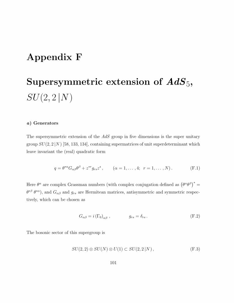
Appendix F
Supersymmetric extension of AdS5,
SU(2, 2 |N )
a) Generators
The supersymmetric extension of the AdS group in five dimensions is the super unitary
group SU(2, 2 |N ) [58, 133, 134], containing supermatrices of unit superdeterminant which
leave invariant the (real) quadratic form
q = θ∗αGαβθβ + z∗rgrsz
s , (α = 1, . . . , 4; r = 1, . . . , N) . (F.1)
Here θα are complex Grassman numbers (with complex conjugation defined as(θαθβ
)∗=
θ∗β θ∗α), and Gαβ and grs are Hermitean matrices, antisymmetric and symmetric respec-
tively, which can be chosen as
Gαβ = i (Γ0)αβ , grs = δrs . (F.2)
The bosonic sector of this supergroup is
SU(2, 2)⊗ SU(N)⊗ U(1) ⊂ SU(2, 2 |N ) , (F.3)
101
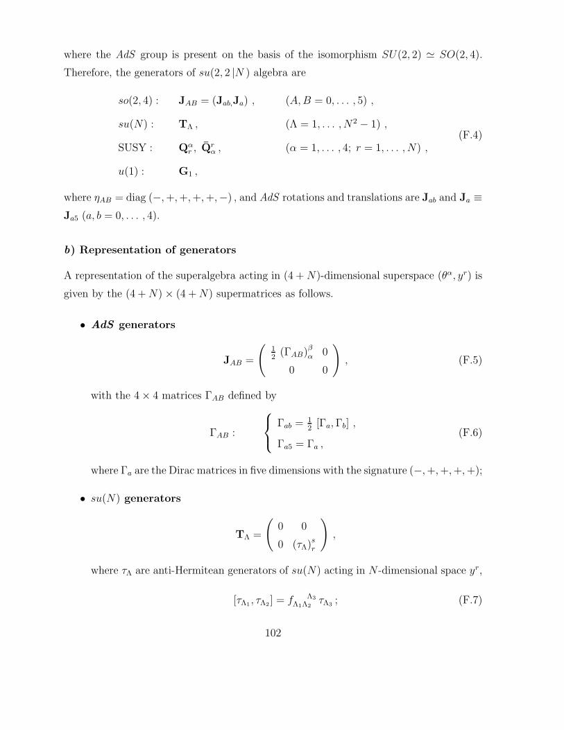
where the AdS group is present on the basis of the isomorphism SU(2, 2) ' SO(2, 4).
Therefore, the generators of su(2, 2 |N ) algebra are
so(2, 4) : JAB = (Jab,Ja) , (A,B = 0, . . . , 5) ,
su(N) : TΛ , (Λ = 1, . . . , N2 − 1) ,
SUSY : Qαr , Qr
α , (α = 1, . . . , 4; r = 1, . . . , N) ,
u(1) : G1 ,
(F.4)
where ηAB = diag (−,+,+,+,+,−) , and AdS rotations and translations are Jab and Ja ≡Ja5 (a, b = 0, . . . , 4).
b) Representation of generators
A representation of the superalgebra acting in (4 +N)-dimensional superspace (θα, yr) is
given by the (4 +N)× (4 +N) supermatrices as follows.
• AdS generators
JAB =
(12
(ΓAB)βα 0
0 0
), (F.5)
with the 4× 4 matrices ΓAB defined by
ΓAB :
Γab = 12
[Γa,Γb] ,
Γa5 = Γa ,(F.6)
where Γa are the Dirac matrices in five dimensions with the signature (−,+,+,+,+);
• su(N) generators
TΛ =
(0 0
0 (τΛ)sr
),
where τΛ are anti-Hermitean generators of su(N) acting in N -dimensional space yr,
[τΛ1 , τΛ2 ] = f Λ3Λ1Λ2
τΛ3 ; (F.7)
102
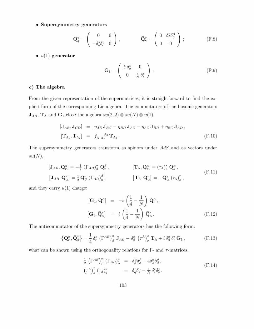
• Supersymmetry generators
Qγq =
(0 0
−δsqδ
γα 0
γ =
(0 δq
rδβγ
0 0
); (F.8)
• u(1) generator
G1 =
(i4δβα 0
0 iNδsr
). (F.9)
c) The algebra
From the given representation of the supermatrices, it is straightforward to find the ex-
plicit form of the corresponding Lie algebra. The commutators of the bosonic generators
JAB, TΛ and G1 close the algebra su(2, 2)⊗ su(N)⊗ u(1),
[JAB,JCD] = ηAD JBC − ηBD JAC − ηAC JBD + ηBC JAD ,
[TΛ1 ,TΛ2] = f Λ3Λ1Λ2
TΛ3 . (F.10)
The supersymmetry generators transform as spinors under AdS and as vectors under
su(N),
[JAB,Qαr ] = −1
2(ΓAB)α
β Qβr , [TΛ,Q
αr ] = (τΛ)s
r Qαs ,[
JAB, Qrα
]= 1
2Qr
β (ΓAB)βα ,
[TΛ, Q
rα
]= −Qs
α (τΛ)rs ,
(F.11)
and they carry u(1) charge:
[G1,Qαr ] = −i
(1
4− 1
N
)Qα
r ,
[G1, Q
rα
]= i
(1
4− 1
N
)Qr
α . (F.12)
The anticommutator of the supersymmetry generators has the following form:
Qα
r , Qsβ
=
1
4δsr
(ΓAB
)αβ
JAB − δαβ
(τΛ)s
rTΛ + i δα
β δsr G1 , (F.13)
what can be shown using the orthogonality relations for Γ- and τ -matrices,
12
(ΓAB
)αβ
(ΓAB)ρλ = δα
β δρλ − 4δα
λδρβ ,(
τΛ)r
s(τΛ)p
q = δrqδ
ps − 1
Nδrsδ
pq .
(F.14)
103
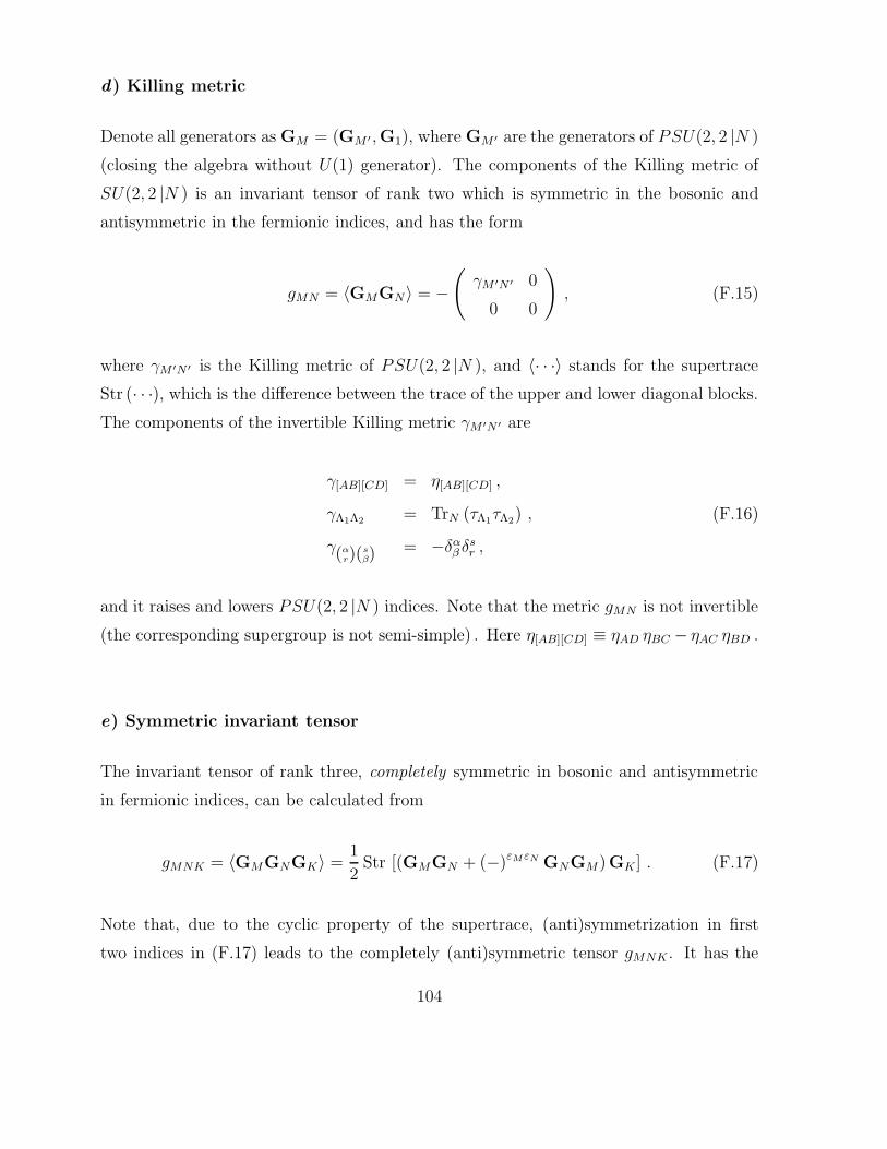
d) Killing metric
Denote all generators as GM = (GM ′ ,G1), where GM ′ are the generators of PSU(2, 2 |N )
(closing the algebra without U(1) generator). The components of the Killing metric of
SU(2, 2 |N ) is an invariant tensor of rank two which is symmetric in the bosonic and
antisymmetric in the fermionic indices, and has the form
gMN = 〈GMGN〉 = −(γM ′N ′ 0
0 0
), (F.15)
where γM ′N ′ is the Killing metric of PSU(2, 2 |N ), and 〈· · ·〉 stands for the supertrace
Str (· · ·), which is the difference between the trace of the upper and lower diagonal blocks.
The components of the invertible Killing metric γM ′N ′ are
γ[AB][CD] = η[AB][CD] ,
γΛ1Λ2 = TrN (τΛ1τΛ2) ,
γ(αr)(
sβ)
= −δαβ δ
sr ,
(F.16)
and it raises and lowers PSU(2, 2 |N ) indices. Note that the metric gMN is not invertible
(the corresponding supergroup is not semi-simple) . Here η[AB][CD] ≡ ηAD ηBC − ηAC ηBD .
e) Symmetric invariant tensor
The invariant tensor of rank three, completely symmetric in bosonic and antisymmetric
in fermionic indices, can be calculated from
gMNK = 〈GMGNGK〉 =1
2Str [(GMGN + (−)εMεN GNGM)GK ] . (F.17)
Note that, due to the cyclic property of the supertrace, (anti)symmetrization in first
two indices in (F.17) leads to the completely (anti)symmetric tensor gMNK . It has the
104
following non-vanishing components:
g[AB][CD][EF ] = − i2εABCDEF ,
gΛ1Λ2Λ3 = −γΛ1Λ2Λ3 ,
g[AB](αr )(s
β)= 1
4(ΓAB)α
β δsr ,
gΛ(αr )(s
β)= 1
2δαβ (τΛ)s
r ,
g1[AB][CD] = − i4η[AB][CD] ,
g1Λ1Λ2 = − iNγΛ1Λ2 ,
g1(αr )(s
β)= i
2
(14
+ 1N
)δαβ δ
sr ,
g111 = −i(
142 − 1
N2
),
(F.18)
where γΛ1Λ2Λ3 ≡ 12TrN (τΛ1 , τΛ2 τΛ3) is the symmetric invariant tensor of rank three for
su(N) and Γ-matrices are normalized so that
Tr4 (Γa Γb Γc Γd Γe) = −4i εabcde ,(εabcde5 ≡ εabcde, ε012345 = 1
). (F.19)
In the special case N = 4, the invariant tensor gMNK of SU(2, 2 |4) simplifies to:
g[AB][CD][EF ] = − i2εABCDEF ,
gΛ1Λ2Λ3 = −γΛ1Λ2Λ3 ,
g[AB](αr )(s
β)= 1
4(ΓAB)α
β δsr ,
gΛ(αr )(s
β)= 1
2δαβ (τΛ)s
r ,
g1M ′N ′ = − i4γM ′N ′ ,
(F.20)
with g111 = 0 and the PSU(2, 2 |4) Killing metric γM ′N ′ given by (F.16).
105
Appendix G
Supergroup conventions
Let GM are supermatrices representing the generators of a Lie supergroup. They satisfy
the superalgebra
[GM ,GN ] = f KMN GK , (G.1)
where the commutators defined by [GM ,GN ] ≡ GMGN − (−)εMεN GNGM and the num-
bers εM ≡ ε (GM) are 0 for bosonic and 1 for fermionic generators (modulo 2). Summation
convention does not apply to (−)ε factors. The generators satisfy the generalized Jacobi
identity
(−)εMεK [[GM,GN ] ,GK ] + (−)εMεN [[GN,GK ] ,GM ] + (−)εKεN [[GK,GM ] ,GN ] = 0 ,
(G.2)
what in terms of the structure constants stands for
(−)εMεK f SMN f L
SK + (−)εMεN f SNK f L
SM + (−)εKεN f SKM f L
SN = 0 . (G.3)
The associated connection 1-form is A = AMGM , where the components AM are
Grassmann even fields (bosons) if εM = 0 and Grassmann odd fields (fermions) if εM = 1.
Then one says that the corresponding generators are bosonic and fermionic as well. Co-
variant derivatives act on a Lie-valued form α as Dα = dα+[A, α] , where the commutator
of a p-form α and a q-form β is generalized to [α, β] ≡ αβ − (−)pq (−)εαεβ βα .
Denote the invariant multilinear form (supertrace) by 〈· · · 〉, which is antisymmetric
for fermionic generators. Then the Killing metric, gMN , and the invariant tensor of rank
106
three, gMNK , are
gMN = 〈GMGN〉 = Str (GMGN) ,
gMNK = 〈GMGNGK〉 = 12Str ([GMGN + (−)εMεN GNGM ]GK) .
(G.4)
The invariant tensors f KMN , gMN and gMNK are Grassmann even variables, ε (gMN) =
εM + εN = 0, etc., and they satisfy the identities
f SMK gSN − gMS f
SKN = 0 ,
gMNS fS
LK − gMSK fS
NL − (−)εLεN gSNK fS
ML = 0 .(G.5)
The above identities follow from the definition of commutator and the cyclic property of
supertrace.
A symmetric tensor TM1···Mn of rank n is defined by an element of Lie algebra T, as
TM1···Mn = 〈GM1 · · ·GMnT〉 . (G.6)
The identities (G.5) are equivalent to DgMN = 0 and DgMNK = 0.
Hamiltonian formalism. Hamiltonian formalism can be generalized to the systems
containing fermions [99], [124]–[127]. If zA are local coordinates on the phase space, then
the Poisson bracket (PB) of functions F (z) and G (z) is
F,G =∂RF
∂zAωAB ∂LG
∂zB, (G.7)
where ∂R/∂zA and ∂L/∂zA stand for right and left derivatives, respectively. The basic
PB arezA, zB
= ωAB. The convention that all derivatives are left is adopted (∂/∂z ≡
∂L/∂z):
δF = δzA ∂F
∂zA. (G.8)
The PBs (G.7) are antisymmetric for bosons and symmetric for fermions, and they satisfy
the generalized Jacobi identity (G.2).
Particularly, for canonical variables zA =(AM
µ (x), πµM(x)
), the PB become
F (x), G (x′) = (−)εF εM
∫d4y
[∂F (x)
∂AMµ (y)
∂G(x′)∂πµ
M (y)− (−)εM
∂F (x)
∂πµM (y)
∂G(x′)∂AM
µ (y)
], (G.9)
107
with the basic PBs
πµ
M (x), ANν (x′)
= −δµ
ν δNM δ(4) (x− x′) = − (−)εM
AM
µ (x), πνN (x′)
. (G.10)
The canonical Hamiltonian has the form
H =
∫dx(πµ
M AMµ − L
), (G.11)
and the corresponding Hamilton equations are
AMµ = (−)εM
δH
δπµM
≈AM
µ , H,
πµM = − δH
δAMµ
≈ πµM , H . (G.12)
Using definitions (G.9) and (G.11), it is straightforward to find the generalization of
generators of local symmetries, as well as to introduce Dirac brackets defining a reduced
phase space.
108
Appendix H
Killing spinors for the AdS5
space-time
The AdS space-time can be given by the metric
ds2AdS = `2
(dr2 + e2rηnm dx
ndxm), ηnm = (−,+,+,+,+) , (H.1)
with the local coordinates xµ = (t, r, xn), where x1 = r and xn = (t, xn). The correspond-
ing vielbein (ea) and the spin-connection (ωab) are given by
e1 = `dr , ωn1 = 1`en = erdxn ,
en = `erdxn , ωnm = 0 ,(H.2)
so that the AdS connection takes the form
W =1
2`eaΓa +
1
4ωabΓab =
1
2`
[e1Γ1 + enΓn (1 + Γ1)
]. (H.3)
The Killing spinors εα are solutions of the Killing equation
Dε = (d+ W) ε = 0 , (H.4)
which for (H.3) splits to the system of the following partial differential equations(∂r +
1
2Γ1
)ε = 0 , (H.5)
[∂n + er Γn (1 + Γ1)] ε = 0 . (H.6)
109
In the ansatz1
ε = h−1(r) Θ−1(xn) ε0 , (H.7)
where εα0 is a constant spinor and h,Θ ∈ SO(2, 4), the equation (H.5) has the solution
h−1(r) = e−r2
Γ1 . (H.8)
Then the equations (H.6) reduce to
[∂nΘ−1 + Cn Θ−1] ε0 = 0 ,
Cn ≡ erer2
Γ1Γn (1 + Γ1) e− r
2Γ1 .
(H.9)
Using the identity
er2
(1+Γ1) = 1 +1
2(1 + Γ1) (er − 1) , (H.10)
the coefficients Cn become
Cn = Γn (1 + Γ1) . (H.11)
Therefore, the general solution of the equation (H.9) is
Θ−1 (xn) = e−xnΓn(1+Γ1) = 1− xnΓn (1 + Γ1) , (H.12)
where it was used that the matrices Γn (1 + Γ1) are nilpotent. Therefore, from (H.7),
(H.8) and (H.12), the AdS Killing spinor has the form [135]
ε = e−r2
Γ1 [1− xnΓn (1 + Γ1)] ε0 . (H.13)
The norm of ε is defined by ‖ε‖2 ≡ εε, where ε = ε†Γ0. Using Γ†n = Γ0ΓnΓ0 and Γ†1 = Γ†1,
as well as the Clifford algebra of Γ-matrices, one obtains
‖ε‖2 = ε0 [1 + xn (1− Γ1) Γn] [1− xnΓn (1 + Γ1)] ε0 = ‖ε0‖2 . (H.14)
Therefore, the spinor ε given by (H.13) has a constant positive norm, ‖ε‖ = ‖ε0‖ > 0.
1For F = 0, the gauge field is a pure gauge, A = g−1dg, and the solution of the Killing equation
Dε = (d + A) ε = 0 is ε = g−1ε0.
110
Bibliography
[1] J. Wess and B. Zumino, Phys.Lett. B37 (1971) 95.
[2] S. P. Novikov, Usp. Math. Nauk. 37 (1982) 3.
[3] E. Witten, Commun. Math. Phys. 92 (1984) 455.
[4] J. Erlich and D. Z. Freedman, Phys. Rev. D55 (1977) 6522.
[5] B. Zumino, Nucl. Phys. B239 (1984) 477.
[6] J. Manes, R. Stora and B. Zumino, Commun. Math. Phys. 102 (1985) 157.
[7] A. Bogojevic, O. Miskovic and B. Sazdovic, Abelian Bosonization, the Wess-Zumino
Functional and Conformal Symmetry. E-Print Archive: hep-th/9811001.
[8] A. Bogojevic, O. Miskovic and B. Sazdovic, The Role of Conformal Symmetry in
Abelian Bosonization of the Massive Thirring Model, Talk given at the 11th Yu-
goslav Simposium on Nuclear and particle Physics, Studenica, Yugoslavia (1988).
E-Print Archive: hep-th/9810120.
[9] E. Witten, Nucl. Phys. B311 (1988) 46.
[10] E. Witten, Commun. Math. Phys. 121 (1989) 351.
[11] S. C. Zhang, T. H. Hansson and S. Kivelson, Phys. Rev. Lett. 62 (1989) 82.
[12] E. Witten, Nucl. Phys. B223 (1983) 422.
[13] K. Gawedzki and A. Kupiainen, Phys. Lett. B215 (1988) 119.
111
[14] K. Gawedzki and A. Kupiainen, Nucl. Phys. B320 (1989) 625.
[15] D. Karabali and H. J. Schnitzer, Nucl. Phys. B329 (1990) 649.
[16] G. Moore and N. Seiberg, Phys. Lett. B220 (1989) 422.
[17] S. Elitzur, G. Moore, A. Schwimmer and N. Seiberg, Nucl. Phys. B326 (1989) 108.
[18] T. Regge and C. Teitelboim, Ann. Phys. (N.Y.) 88 (1974) 286.
[19] L. F. Abbott and S. Deser, Nucl. Phys. B195 (1982) 76.
[20] L. F. Abbott and S. Deser, Phys. Lett. B116 (1982) 259.
[21] A. M. Polyakov, Mod. Phys. Lett. A2 (1987) 893.
[22] V. G. Knizhnik, A. M. Polyakov and A. B. Zamolodchikov, Mod. Phys. Lett. A3
(1988) 819.
[23] E. Abdalla, M. C. B. Abdalla, J. Gamboa and A. Zadra, Phys. Lett. B273 (1991)
222.
[24] P. Forgacs, A. Wipf, J. Balog, L. Feher and L. O’Raifeartaigh, Phys. Lett. B227
(1989) 214.
[25] O. Coussaert, M. Henneaux and P. van Driel, Class. Quant. Grav. 12 (1995) 2961.
[26] A. Achucarro and P. K. Townsend, Phys. Lett. B180 (1986) 89.
[27] E. Witten, Nucl. Phys. B311 (1988) 46.
[28] S. Carlip, Quantum Gravity in 2+1 Dimensions (Cambridge University Press,
1998).
[29] J. D. Brown and M. Henneaux, Commun. Math. Phys. 104 (1986) 207.
[30] M. T. Grisaru, Phys. Lett. B66 (1977) 75.
[31] S. Deser and J. H. Kay, Phys.Lett. B76 (1978) 189.
112
[32] M. F. Sohnius, Phys. Rep. C128 (1985) 39.
[33] C. M. Hull and B. Spence, Nucl. Phys. B345 (1990) 493.
[34] M. Banados, K. Bautier, O. Coussaert, M. Henneaux and M. Ortiz, Phys. Rev. Lett.
D58: 085020 (1998).
[35] M. Henneaux, L. Maoz and A. Schwimmer, Ann. Phys. 282 (2000) 31.
[36] E. B. Bogomol’nyi, Sov. J. Nucl. Phys. 24 (1976) 449.
[37] E. Witten, Commun. Math. Phys. 80 (1981) 381.
[38] S. Deser and C. Teitelboim, Phys. Rev. Lett. 39 (1977) 249.
[39] M. Grisaru, Phys. Lett. B73 (1978) 207.
[40] D. Olive and E. Witten, Phys. Lett B78 (1978) 97.
[41] E. Witten, Nucl. Phys. B186 (1981) 412.
[42] K. Viswanathan, Dimensional Reduction and Harmonic Expansions on Coset
Spaces, Proceeding of the Workshop on Kaluza-Klein Theories, Chalk River,
Canada, ed. H. C. Lee, World Scientific, Singapore (1983).
[43] R. Floreanini and R. Percacci, Phys. Lett. B224 (1989) 291.
[44] R. Floreanini, R. Percacci and R. Rajaraman, Phys. Lett. B231 (1989) 119.
[45] A. Chamseddine, Phys. Lett. B233 (1989) 291.
[46] V. P. Nair and J. Schiff, Phys. Lett. B246 (1990) 423.
[47] V. P. Nair and J. Schiff, Nucl. Phys. B371 (1992) 329.
[48] A. Chamseddine, Nucl. Phys. B346 (1990) 213.
[49] M. Banados, R. Troncoso and J. Zanelli, Phys. Rev. D54 (1996) 2605.
[50] R. Troncoso and J. Zanelli, Phys. Rev. D58: R101703 (1998).
113
[51] R. Troncoso and J. Zanelli, Int. J. Theor. Phys. 38 (1999) 1181.
[52] M. Hassaine, R. Olea and R. Troncoso, New N = 2 Supergravity With Local
Poincare Invariance in Nine Dimensions, Report-No: CECS-PHY-02-06,
E-Print Archive: hep-th/0210116.
[53] R. Troncoso and J. Zanelli, Class. Quant. Grav. 17 (2000) 4451.
[54] M. Banados, L. J. Garay and M. Henneaux, Phys. Rev. D53 (1996) 593.
[55] M. Banados, L. J. Garay and M. Henneaux, Nucl. Phys. B476 (1996) 611.
[56] R. Troncoso and J. Zanelli, Chern-Simons Supergravities with Off-Shell Local Super-
algebras, in “Black Holes and Structre of the Universe”, editors C. Teitelboim and
J. Zanelli (World Scientific, Singapore, 1999). E-Print Archive: hep-th/9902003.
[57] A. Losev, G. Moore, N. Nekrasov and S. Shatashvili, Nucl. Phys. Proc. Suppl. 46
(1996) 130.
[58] O. Chandıa, R. Troncoso and J. Zanelli, Dynamical Content of Chern-Simons
Supergravity, Talk given at The Second La Plata Meeting on Trends in The-
oretical Physics, Buenos Aires, Argentina, November 1998. E-Print Archive:
hep-th/9903204.
[59] P. A. M. Dirac, Lectures on Quantum Mechanics (Yeshiva University, New York,
1964).
[60] C. Batlle, J. Gomis, J. M. Pons and N. Roman-Roy, J. Math. Phys. 27 (1986) 2953.
[61] J. A. Garcıa and J. M. Pons, Int. J. Mod. Phys. A13 (1998) 3691.
[62] R. Di Stefano, Phys. Rev. D27 (1983) 1752.
[63] J. M. Pons, D. C. Salisbury and L. C. Shepley, Phys. Rev. D62 (2000) 064024.
[64] O. Miskovic and B. Sazdovic, Mod. Phys. Lett. A17 (2002) 1923.
114
[65] O. Miskovic and J. Zanelli, Irregular Hamiltonian Systems, Proceedings of the
XIII Chilean Symposium of Physics, Concepcion, Chile, November 2002. E-Print
Archive: hep-th/0301256.
[66] O. Miskovic and J. Zanelli, J. Math. Phys. 44 (2003) 3876.
[67] J. Saavedra , R. Troncoso and J. Zanelli, J. Math. Phys. 42 (2001) 4383.
[68] J. Saavedra , R. Troncoso and J. Zanelli, Rev. Mex. Fis. 48 (2002) SUPPL 387-89.
[69] O. Miskovic, R. Troncoso and J. Zanelli, Dynamics and Charge Algebra for Chern-
Simons-AdS 5 Supergravity. Report-No: CECS-PHY-04/02. (in preparation)
[70] B. Sazdovic, Phys. Lett. B352 (1995) 64.
[71] H. Sugawara, Phys. Rev. 170 (1968) 2019.
[72] C. Sommerfield, Phys. Rev. 176 (1968) 2019.
[73] P. Goddard and D. Olive, Int. J. Mod. Phys. A1 (1986) 303.
[74] A. A. Belavin, A. M. Polyakov and A. B. Zamolodchikov, Nucl. Phys. B241 (1984)
333.
[75] P. Di Francesco, P. Mathieu and D. Senechal, Conformal Field Theory (Springer-
Verlag, New York, 1997).
[76] P. West, Introduction to Supersymmetry and Supergravity (World Scientific, Singa-
pore, extended second edition, 1990).
[77] A. M. Polyakov and P. B. Wiegmann, Phys. Lett. B131 (1983) 121.
[78] B. Sazdovic, The WZNW Term in the Quantization of Theories with Anomalies,
Proceedings of Danube Workshop ’93, p.34 (Editors A. R. Bogojevic, T. Vukasinac,
Belgrade, Yugoslavia, 1993).
[79] P. Di Vecchia, V. G. Knizhnik, J. L. Petersen and P. Rossi, Nucl. Phys. B253 (1985)
701.
115
[80] E. Abdalla and M. C. B. Abdalla, Phys. Lett. B152 (1985) 59.
[81] P. Ramond, Phys. Rev. D3 (1971) 2415.
[82] A. Neveu and J. H. Schwarz, Nucl. Phys. B31 (1971) 86.
[83] A. Neveu and J. H. Schwarz, Phys. Rev. D4 (1971) 1109.
[84] E. Bergshoeff, S. Randjbar-Daemi, A. Salam, H. Sarmadi and E. Sezgin, Nucl. Phys.
B269 (1986) 77.
[85] S. James Gates Jr. and H. Nishino, Class. Quantum. Grav. 3 (1986) 391.
[86] S. V. Ketov, Class. Quantum. Grav. 4 (1987) 1163.
[87] L. Brink, S. Deser, B. Zumino, P. Di Vecchia and P. S. Howe, Phys. Lett. B64
(1976) 435.
[88] L. Brink , P. Di Vecchia and P. S. Howe, Phys. Lett. B65 (1976) 471.
[89] S. Deser and B. Zumino, Phys. Lett. B65 (1976) 369.
[90] M. Blagojevic, D. S. Popovic and B. Sazdovic, Mod. Phys. Lett. A13 (1998) 911.
[91] M. Blagojevic, D. S. Popovic and B. Sazdovic, Phys. Rev. D59: 044021 (1999).
[92] A. Mikovic and B. Sazdovic, Mod. Phys. Lett. A10 (1995) 1041.
[93] A. Mikovic and B. Sazdovic, Mod. Phys. Lett. A12 (1997) 501.
[94] D. S. Popovic and B. Sazdovic, Mod. Phys. Lett. A16 (2001) 589.
[95] B. Sazdovic, Phys. Rev. D62: 045011 (2000).
[96] B. Sazdovic, Mod. Phys. Lett. A17 (2002) 1923.
[97] E. D’Hoker and D. H. Phong, Rev. Mod. Phys. 60 (1988) 91.
[98] P. A. M. Dirac, Can. J. Math. 3 (1951) 1.
116
[99] M. Henneaux and C. Teitelboim, Quantization of Gauge Systems (Princeton Uni-
versity Press, Princeton, 1992).
[100] C. Leiva and M. S. Plyushchay, Ann. Phys. (2003) 307.
[101] L. Castellani, Ann. Phys. (N. Y.) 143 (1982) 357.
[102] M. Blagojevic, Gravity and Gauge Symmetries (Institute of Physics Publishing,
London, 2001).
[103] W. Siegel, Nucl. Phys. B238 (1984) 307.
[104] M. Henneaux and C. Teitelboim, Consistent Quantum Mechanics of Chiral p-forms,
in “Quantum Mechanics of Fundamental Systems 2”, editors C. Teitelboim and J.
Zanelli (Plenum Press, New York, 1989).
[105] M. S. Plyushchay and A. V. Razumov, Dirac versus reduced phase space quantiza-
tion, Proceedings of Geometry of Constrained Dynamical Systems, p. 239 (Cam-
bridge, 1994). E-Print Archive: hep-th/9412137.
[106] M. S. Plyushchay and A. V. Razumov, Int. J. Mod. Phys. A11 (1996) 1427.
[107] G. Grignani, M. S. Plyushchay and P. Sodano, Nucl. Phys. B464 (1996) 189.
[108] K. S. Nirov and M. S. Plyushchay, Nucl. Phys. B512 (1998) 295.
[109] T. R. Allcock, Phil. Trans. R. Soc. (Lond.) 279 (1975) 33.
[110] R. Cawley, Phys. Rev. Lett. 42 (1979) 413.
[111] M. Banados, M. Henneaux, C. Teitelboim and J. Zanelli, Phys. Rev. D48 (1993)
1506.
[112] J. D. Brown and M. Henneaux, J. Math. Phys. 27 (1986) 489.
[113] M. Banados, Black Holes of Constant Curvature, in “Recent developments in theo-
retical and experimental general relativity, gravitation, and relativistic field theories,
Pt.B” (Jerusalem, 1997). E-Print Archive: gr-qc/9710052.
117
[114] M. Banados, C. Teitelboim and J. Zanelli, Phys. Rev. D49 (1994) 975.
[115] Rong-Gen Cai and Kwang-Sup Soh, Phys. Rev. D59: 044013 (1999).
[116] J. Crisostomo, R. Troncoso and J. Zanelli, Phys. Rev. D62: 084013 (2000).
[117] R. Aros, R. Troncoso and J. Zanelli, Phys. Rev. D63: 084015 (2001).
[118] O. Coussaert and M. Henneaux, Phys. Rev. Lett. 72 (1994) 183.
[119] P. A. M. Dirac, Can. J. Math. 2 (1950) 129.
[120] P. A. M. Dirac, Proc. R. Soc. (Lond.) A246 (1958) 326.
[121] J. L. Anderson and P. G. Bergman, Phys. Rev. 83 (1951) 1018.
[122] P. G. Bergman, I. Goldberg, A. Janis and E. Newman, Phys. Rev. 103 (1956) 807.
[123] P. G. Bergman, Rev. Mod. Phys. 33 (1961) 510.
[124] F. A. Berezin and M. S. Marinov, Ann. Phys. 104 (1977) 336.
[125] R. Casalbuoni, Nuovo Cimento A33 (1976) 115.
[126] R. Casalbuoni, Nuovo Cimento A33 (1976) 389.
[127] J. L. Gervais and B. Sakita, Nucl. Phys. B64 (1971) 632.
[128] A. J. Hanson, T. Regge and C. Teitelboim, Constrained Hamiltonian Systems (Ac-
cademia Nazionale dei Lincei, Rome, 1976).
[129] K. Sundermeyer, Constrained Dynamics (Springer Lecture Notes 169, Berlin, 1982).
[130] M. Henneaux, Phys. Rept. 126 (1985) 1.
[131] A. W. Wipf, Hamilton’s Formalism for Systems with Constraints, Lectures given at
the Seminar “The Canonical Formalism in Classical and General relativity” (Bad
Honnef, Germany, 1993). E-Print Archive: hep-th/9312078.
118
[132] E. Inonu, Contractions of Lie Groups and Their Representations, “Group Theoret-
ical Concepts and Methods in Elementary Particle Physics” (Ed F. Gursey; Gordon
and Breach, New York, 1964, p.391).
[133] W. Nahm, Nucl. Phys. B135 (1978) 149.
[134] J. Strathdee, Int. J. Mod. Phys. A2 (1987) 273.
[135] H. Lu, C. N. Pope and P. K. Townsend, Phys. Lett. B391 (1997) 39.
[136] R. Aros, C. Martinez, R. Troncoso and J. Zanelli, JHEP 0205 (2002) 020.
119