I

I.IIIIIIII_IIIIIII.eI

ON THE DISTRIBUTION OF STATISTICS SUITABLE FOR EVALUATINGRAINFALL STIMULATION EXPERIMENTS

by

K. R. Gabriel, Hebrew University, Jerusalemand University of North Carolina, Chapel Hill

andPaul Feder, Stanford University

Institute of Statistics Mimeo Series No. 520

April 1967

This work was supported in part by the National Institutesof Health (Institute of General Medical Sciences) Grant No.GM-12868-03.

DEPARTMENT OF BIOSTATISTICS

UNIVERSITY OF NORTH CAROLINA

Chapel Hill, N. C.

I

I.IIIIIII1_III

III.-I

ON THE DISTRIBUTION OF STATISTICS SUITABLE FOR EVALUATINGRAINFALL STIMULATION EXPERIMENTS*

by

K. R. Gabriel, Hebrew University, Jerusalemand University of North Carolina, Chapel Hill

and

Paul Feder, Stanford University

ABSTRACT

Two randomization tests of the null hypothesis in cloud seeding

experiments are compared - the Wilcoxon-Mann-Whitney test and a test based

on an average ratio of seeded to non-seeded amounts of precipitation.

Data from the Israeli experiment suggest that the latter test is relative­

ly more sensitive to apparent effects of seeding. The significance level

of this test may be estimated by Monte Carlo methods or approximated by

using the asymptotic normal distribution of the average ratio. Sampling

trials show that this approximation is adequate only when the experiment

is of several years' duration.

1. PROBLEMS OF STATISTICAL EVALUATION OF RAINFALL STIMULATION EXPERIMENTS.

The statistical evaluation of randomized rainfall stimulation experiments

raises problems of choice of valid and suitable methods of analysis. Most stand-

ard statistical techniques are not applicable to such experiments since precipi-

tation data do not generally fit the common textbook assumptions. Distributions

of amounts of precipitation, especially for short periods such as 24 hours, are

usually discontinuous at zero and have most pronounced tails. The discontinuity

is due to a positive probability of no rainfall at all, and the tails show the

presence of occasional very extreme amounts. Furthermore, measurements of pre-

cipitation are not independent either in space or in time, but there exist strong

* This work was supported in part by the National Institutes of Health (Instituteof General Medical Sciences) Grant No. GM-12868-03.

-2 -

correlations between stations which are scores of miles apart as well as appre­

ciable dependence of precipitation on successive days. This lack of "good be­

haviour" of the data is especially troublesome when complex experimental designs

are used, such as cross-over designs with random daily allocation of seeding to

alternate areas and when detailed and sensitive statistical analyses are required,

e.g., when concomitant variables are to be taken into account.

A further difficulty in applying standard statistical techniques is that

the form of possible seeding effects is not known but may well be most irregular.

Considerable differences in the outcomes of different rainfall stimulation ex-

periments point to the existence of factors, not hitherto identified, which may

sometimes further the effectiveness of cloud seeding but perhaps inhibit it at

other times (Neyman and Scott [8]). A number of findings suggest that seeding

may be highly effective on some occasions but have little or no effect on many

other occasions (Siliceo et al. [10], Gabriel [4]). Since so little is known

about the alternative one should be testing against, it is not only doubtful

whether standard techniques are valid but it is difficult to decide what a good

technique is. (For the derivation of optimal techniques under certain simple

assumptions, see Neyman and Scott [7]).

Unless a satisfactory parametric model of precipitation becomes available,

i.e., one which takes account of all the irregularities and dependences noted

above, the safe course is to use randomization tests. (For an earlier discussion

of the need for non-parametric tests, see Adderley [1]). Such tests compare a

summary statistic based on the experimental results under the actual randomized

allocation of treatments with all possible values this statistic might have

assumed for the same experimental results had the allocation been different.

To be specific, for each possible allocation under the randomization scheme,

I

.­IIIIIII

_IIII'II:II-.I

I

I.IIIIIII

IIIIIII••I

the observed experimental data are considered afresh and the resulting statistic

compared with that found under the allocation used. This is a valid comparison

under the null hypothesis that seeding has no effect, for in that case the same

rainfalls would have occurred, no matter what the allocation. Clearly, random-

ization tests do not require any assumptions about the distribution and dependence

of the precipitation data, and therefore provide valid analyses of rainfall

experiments.

Different randomization tests are obtained by using this principle with

different statistics. For example, one may take the difference between mean

values on treated observations and on control observations, and compare the ex-

perimental difference with similar differences obtained by other allocations of

the same data. Alternatively, one might take the difference between medians, or

mean ranks, or proportions of observations above some constant, etc .. Each com-

parison statistic will yield a randomization test. For certain statistics the

distribution over all allocations can be derived mathematically, and critical

values for significance testing have been computed and tabulated. A well-known

example is the WMW (Wilcoxon-Mann-Whitney) test whose statistic is the number

of pairs consisting of a treated and a control observation, for which the treat-

ed observation has a larger variable value than the control observation.

2. THE TWO TESTS IN THE ISRAELI EXPERIMENT.

The Israeli rainfall stimulation experiment uses a cross-over design

with daily random allocation of seeding to either the North or the Centre of

Israel. (For detailed descriptions of the experiment, see Gabriel [3], [4],

[5]) .

-4-

Most analyses of this experiment are confined to rainy days - defined

as having some precipitation in the always unseeded buffer area between the

I_.I

ing effects.

denote the mean amounts of precipitation per station in the North and the Centre

North and the Centre. In effect some 987. of all precipitation occurs on such

days so that the omission of the other, dry,. days is unlikely to hide any seed- IIII

The random allocation variable 8. is defined as 1 if seeding is~

For a day indexed by subscript i, out of a total of N days, x. and y.~ ~

allocated to the North and as 0, i.e., 1 - 8. = 1, if seeding is allocated to~

respectively.

where ~ .. indicates whether the ith day's variable exceeds the jth day's variable.~J

In the Israeli experiment x.-y. was chosen as experimental variable so that~ ~

the Centre. With this notation, the WMW test uses the count statistic

N NU'" L: L: 8. (1-8 . )¢l. .

i=l j=l ~ J ~J(1)

II

_II

1 if xi-Yi > x j -Yj

$ .. = if x. -yo = x j - Yj (2)~J ~ ~

0 if xi-Yi < X.-y ..J J

Note that even though the x.-y. are not independent and identically distributed~ ~

under the hypothesis of no seeding effects, the WMW test is still valid since

IIII

the seeding allocation was determined by randomization.

This statistic is easily computed and its distribution has been tabulated

in detai1*. The WMW test can, therefore, be used in over-all analyses of entire

* See, for example, the tables by Owen [9]. For large samples an asymptoticapproximation is available.

II-.I

I

I.IIIIII

-5 -

experiments as well as for detailed investigations which require testing in each

of many categories of days. Such detailed analyses are of considerable importance

in increasing sensitivity by using categories defined by well correlated concom-

itant variables (Gabriel [4J) and in providing breakdowns from which one may learn

under what conditions seeding may be more or less effective (Neyman and Scott [8J).

Alternatively, a randomization test may be based on a quantitative meas-

ure of apparent seeding effect. The choice of a suitable measure will be guided

by simplicity and by what one considers relevant as a useful or economically

valuable effect. A ratio of amounts of precipitation under seeding to amounts

in the absence of seeding may serve this purpose. In cross-over designs such a

ratio can be obtained as the geometric mean of the seeded to unseeded ratios of

both experimental areas. In the above notation, one may write the total amountsI1_I

as

in North:Nl: e.x.

i=l ~ ~seeded;

Nl: (l-e. )x.

i=l ~ ~unseeded,.

This average ratio is defined as R, where*

II

in Centre:NL: (l-e.)y.

i=l ~ ~seeded;

NL: e.y.

i=l ~ ~unseeded.

II

R2 = [~ e. x. / ~ (l-e.) xJr~ (l-e.) y. / ~ e. yJi=l ~ ~/ i=l ~ 1L.=1 ~ ~/ i=l ~ ~

(3)

II

••I

(R has been referred to as the Root-Doub1e-Ratio by the Australian cloud seed-

int team, who seem to have been the first to use it - Adderley and Twomey [2]).

One notices that each day's e. = 1 or 1 - e. = 1 appears twice in the expression~ ~

* If all e's are equal, R may be arbitrarily defined as 1.

-6 -

for R, once in the numerator with one of the variables x, y and once in the de-

nominator with the other variable. And since precipitation in the North and the

Centre, i. e., x and y, is highly correlated (r=.8), this ensures that variations

due to the random allocation of seeding will not greatly affect the statistic

R. (An. approximation to R is discussed in the Appendix).

The statistic R is an average ratio, but its use must not be understood

to imply that the actual effect of cloud seeding on precipitation is multipli-

cative. R is an average, and a particular value of R might be the result of a

variety of effects on different days of the experiment.

In comparing the two statistics it is clear that R has the advantage of

depending directly on amounts of seeded versus unseeded rainfall, whereas U de-

pends on these amounts only indirectly through the ranking of the differences

(x.-y.) - (x.-y.). If none of these differences are particularly large, either~ ~ J J

positively or negatively, as compared with the rest, it will not matter much

that ranks are used instead of actual values, and the WMW statistic may be as

appropriate as R but simpler to use. Indeed, the WMW test is known to be power-

ful in many standard situations. For these reasons the WMW test was originally

chosen for the analysis of the Israeli experiment.

If, however, effects of seeding vary a great deal from day to day, i.e.,

if seeding has little or no effect on most days but on a few days it has very

large effects, this will hardly affect the ranking of the (x -y ) - (xJ'-Yj) dif­i i

ferences even though some of them become extremely large. The WMW test will be

quite insensitive to effects of this kind, but the R statistic will show them

clearly. A hypothetical example will illustrate this:

II

e·IIIIIIII

III

_IIIIIIIIe.I

i 1 2 3 4 5 6 7 8 9 10 11 12 13 14 15 16

e. 1 0 o 100 1 1 0 1 0 0 1 1 0 01

X. 5 7 3 4 6 9 25 7 5 6 3 5 17 8 7 71

Yi 6 6 12 4 5 7 8 8 4 8 10 4 5 8 5 7

R =.J (72/52)(60/47) = 1.33

I

I.IIIII

16L: e. = 7,

i=l 1

16L: e.x. = 72,

i=l 1 1

-7-

16L: (1-e.) x. = 52,

i=l 1 1

16L: e.Y. = 47,

i=l 1 1

U = 29.

16L: (1-e.)y. = 60

i=l 1 1

III_IIIIIIII·

I

(Approximation - see Appendix - 1 + 2(S-T) = 1 + 2(72~~2 - 47~~0) = 1.28).

The median values under the null seeding effect hypothesis are Med R = 1 and

Med U = 7 )(' 9/2 = 31. 5, so that the two statistics deviate from their medians

in different directions. R indicates positive seeding' effects because of the

few apparently large effects (on days 3, 7, 11 and 13) whereas U indicates the

contrary because all twelve other days had apparent small negative effects or

no effects at all.

Another drawback of the WMW technique is that it is merely a test of

significance and does not provide a quantitative estimate of the size of seeding

effects. To obtain estimates and confidence bounds one must have recourse to

rather cumbersome iterative techniques whose results lean heavily on one's

assumptions regarding the form (e.g., additive, multiplicative, etc.) of the

effects - assumptions which unfortunately have little to be based upon (Gabriel

[4], section 5.1).

Variation of the statistic R from allocation to allocation depends on

the actual amounts of precipitation observed during the experiment. It can

therefore not be studied generally as was the U statistic of the WMW test.

'j

-8-

A Gomplete enumeration of values of R obtained under all possible allocations

is not practical either, even with an electronic computer (with 300 rainy days

3002 . values would have had to be computed). However, one may use the Monte

Carlo technique to sample from all these allocations and thereby obtain an

estimate,of the probability of exceeding the actually observed R, RO say, by

chance. Such sampling is readily performed on an electronic computer. For

each sample a (pseudo) random allocation is generated and the experimental data

used to compute the sample value of R. The proportion of sample R values which

exceed the experimental value RO

is an estimate of ~ = P(R > RO). Simple random

sampling theory applies, so that the estimate is unbiased and has variance (l-~)~/n

where n is the number of samples generated. A few hundred samples usually suffice

to give a fairly good idea of the level of significance and the cost of generat-

ing the~ on a modern computer is negligible as compared with the expenses involved

in a cloud seeding experiment.

For the data of the entire Israeli experimen~ as well as for a number

of categories of days separatelY,Monte Carlo trials of several hundred samples

each were run on the Hebrew University's I.B.M. 7040 computer. The resulting

estimates of significance levels by the randomization test are compared in Table 1

with those obtained by the WMW test. (The "R-asymptotic" levels of significance

of. Table 1 are discussed in section 3, below. The 1 + 2(S-T) approximation to R

is discuss~d in the Appendix).

Each row of Tables land 2 contains the results of different and indepen-

dent. Monte Carlo randomization samples, but the same daily rainfall data was used

repeatedly. Thus, there are 400 and then another 200 independent randomizations

on the same 1961-5 data, 500 more randomizations run after the 1965/6 season's

results were added to the data, and a further 400 randomizations for the same

II

IIIIIII

_IIIIIIII-.I

* A detailed description of the dates and groupings in these tables is given else­where (Gabriel [4J, [5J) and is not repeated here as it is not directly relevantto the question of choice of statistics. However, it may be mentioned that theannual periods are mid-October to mid-April (except 1961 which started in Feb­ruary). The split of the 1963/4 season was due to a change in the definition ofthe operational day from an 8 p.m. start and end to an 8 a.m. start and end ofseeding.

Table 1. Significance Levels Attained by Different Tests ­Rainy Days On1y*

-9 -

Number Level of Significance Observed Observed Number ofof

W-M-WR-Random- R-Asymp- R l+2(S-T) Permuta-

Days ization totic tions

1961-6 327 .057 .004 .004 1. 190 1. 174 500

1961-6 (Interior of Regions) 327 .009 .000 .0003 1.273 1. 240 400

1961-5 281 .190 .03 .024 1.155 1. 144 400

.04 200

1961 26 .140 .0725 .OU 1.737 1. 492 400

1961/2 57 .387 .21 .173 1.185 1. 164 400

1962/3 49 .532 .34 .242 1. 102 1.095 400

1963/4A 20 .605 .47 .463 1. 017 1. 017 400

1963/4B 57 .032 .0175 .008 1.376 1.317 400

1964/5 72 .615 .175 .164 1.131 1.123 400

1965/6 46 .015 .0025 .001 1.544 1. 391 400

1961-2 83 .263 .14 .082 1. 244 1.215 200

962-4 126 .165 .12 .074 1.154 1.143 200

1964-6 U8 .133 .02 .014 1. 244 1.213 200

1961-6 Buffer- < -10 26 .123 .130 .085 1.138 1.126 300South

" " -10 :::; < - 5 22 .178 .087 .055 1. 281 1. 243 300

" " - 5 :::; < - 1 27 .055 .027 .008 1.395 1.309 300

" " - 1 :::; < 0 24 .074 .120 .029 1. 415 1.209 300

" " o :::; < 1 81 .855 .130 .058 1. 433 1.355 300

II II 1 :::; < 3 46 .843 .683 .685 0.918 0.936 300

" II 3 :::; < 5 20 . 741 .820 .813 O. 709 O. 700 300

II II 5 :s < 10 35 .008 .047 .008 1.394 1. 293 300

" " 10 < < 20 23 .019 .000 .000 1. 792 1. 507 300

II II 20 :s 23 .189 .220 .163 1.177 1.159 300

II.eIIIIIIIIIIIIII.eI

-10-

days' rainfall in the interior areas which is highly correlated with that in

the entire areas used before. Clearly, in as far as effects of cloud seeding are

apparent, and one test is found more sensitive than another, these different cal-

culations give dependent and very similar results. However, as regards the form

of the distribution of the sample R values, the results are independent from one

row to another, each being based on separate Monte Carlo samples. The same re-

marks apply also to the further repeated use of the same rainfall data in each

of the next four parts of the Tables. As far as Tabl~ 1 is concerned these are

repetitious uses of the same data and must not be mistaken as independent cumula-

tive evidence. The rows and parts of Table 2, on 'the other hand, do provide in-

dependent information on the distribution of R under randomization.

For all seasons together as well as for each season by itself, the signif-

icance levels for the WMW test are seen to exceed the estimates of ~ for the R

randomization test. In so far as the seeding effects observed in this and other

experiments are real and not mere random fluctuations in rainfall, the difference

in the behaviour of the two tests would indicate that the WMW test is indeed less

sensitive to this type of effect than the test using the average ratio. One

II-.IIIIII

_III

would conclude that the WMW test, though valid for rainfall stimulation experi-

ments, is less powerful than the R-randomization test. Clearly, this conclusion Iis meaningful only if there really are seeding effects, whereas if seeding were

completely ineffectual, no one test could be more powerful than another.

Table 1 also shows similar comparisons of levels within categories of

days defined by means of a concomitant variable that is correlated with x-y but

is unaffected by seeding. This variable is the difference in precipitation

amounts between the unseeded buffer and South areas, which lie, respectively,

between the North and Centre experimental areas and South of the Centre area.

IIII-.I

II.e

-11-

No consistent pattern is found between the two levels of significance. For some

categories the WMW level is higher, for other categories the R level is higher.

II

In so far as real seeding effects exist and the above conclusions about the

relative sensitivity of the two tests are meaningful, one would further conclude

that the greater sensitivity of the R-randomization test holds only when all types

Iof days are tested together. Within relatively homogeneous categories of days,

neither test would appear consistently superior to the other.

I3. THE ASYMPTOTIC DISTRIBUTION OF R AND ITS USE.

I When the number N of experimental observations is large, the sampling

I1_

distribution of R may be approximated by asymptotic theory. It is shown in the

Appendix that for large N the distribution of R under random allocation of seed-

ing tends to normality with expectation 1 and variance

II where

Nl:: (x./X-y./y)2 ,

i=l 1 1

(4)

the total amounts and differences over the entire experiment even when the experi-

To find out whether this assumption is tenable for precipitation data

or whether it is vitiated by the occasional occurrences of extreme amounts of

equations (15) and (18» .

(5)N

Y= l:: y.i=l 1

andN

X = l:: x.i=l 1

This asymptotic result holds provided no single value of either xf/X2 0r yf/Y2

or (Xi/X - Yi/y)2 remains appreciable as N increases. In other words, it holds

unless the rainfall amounts x, y and differences i -i on a very few days dominate

ment becomes increasingly long. (The exact conditions are given in the Appendix,

IIIII• eI

-12 -

rain~all, the distribution of sample R values was compared to the asymptotic

normal distribution. Sample R values were obtained by the same Monte Carlo

s,amp.1ing ,described above in connection with Table 1. The results are pre-

sented in Table 2 for data of the entire Israeli experiment as well as for

several separate categories of days.

Tests qf goodness of fit of the asymptotic normal distribution withN

mean 1 and variance ~ (x.!X-y.!y)2 show no significant deviations when thei=l ~ ~

data for the entire 1961-5 or 1961-6 period of the experiment are analyzed.

However, when R values are obtained separately for each season, the fit is

significantly poor - sum of chi-square statistics 389.00 with 133 d.f;. For

pairs of seasons the fit is not good - sum of chi-square statistics 73.40 with

57 d.f .. , One may conclude that asymptotic theory gives a good approximation

when N is as large as 300 rainy days (5-6 seasons), that it is doubtful for

lQO~odd ~ainy days (2 seasons), and that it is clearly inadequate for as few

as 50 or,so days (single seasons).

Monte Carlo trials have also been carried out within ten categories of

days defined by the buffer-South difference. The number of days per category

was about N = 30, and the fit of the sample R distribution to the asymptotic

normal was very poor - sum of chi-square statistics 427.4 with 190 d.f .. Clearly,

for, this size of N the asymptotic approximation is inadequate even within rela-

tiv~lyhomogeneous categories of days.

~4rther details of the sampled distributions of R are also presented

;in Table, 2." These ,give some idea of how the sampled distributions of R deviate

from the, asymptotic normal. The distributions of R have slight positive skew-

ness and, a: small positive bias in the expectation. The bias is of the order of

2%tfor: single seasons and of less than 1% for the whole length of the experiment.

II

IIIIIIII

_IIIIIIII-,I

-13-

Table 2. Sampled Distributions of R, Goodness of Fit andOther Characteristics (Rainy Days Only)

t Each distribution of Monte Carlo sample values of R was sortedinto 20 classes for testing of goodness of fit .

* Amounts of precipitation in interior parts of areas only.

Num- Number Chi-squareber of for goodness Prop. Mean Variance Asymptoticof Permuta- of fit (R ~ 1) var1ance 0,3 0,4

Days tions 19 d.Lt

1961-6 327 500 29.2 .52 1. 0051 .0052 .0053 .006 2.81

1961-6']( 327 400 14.1 .51 1. 0034 .0066 .0063 .014 3.16

1961-5 281 400 21. 1 .51 1. 0075 .0061 .0061 .025 3.36

200 23.4 .52 1.0042 .0064 .0061 .027 2.96

1961 26 400 153.7 .49 1. 0739 .1596 .1018 .295 2.91

1961/2 57 400 50.3 .48 1. 0221 .0519 .0387 .174 3.96

1962/3 49 400 62.9 .52 1. 0214 .0262 .0212 .057 2.59

1963/4A 20 400 37.7 .51 1. 0208 .0473 .0352 .092 3.34

1963/4B 57 400 35.1 .50 1.0117 .0285 .0243 .055 2.78

1964/5 72 400 18.1 .49 1. 0025 .0200 .0180 .055 2.99

1965/6 46 400 31.2 .52 1.0131 .0316 .0298 .053 2.57

1961-2 83 200 29.8 .52 1. 0312 .0367 .0307 .066 2.64

1962 -4 126 200 21.2 .56 1. 0163 .0130 .0113 .018 2.84

1964-6 118 200 22.4 .52 1. 0152 .0129 .0122 .028 2.46

1961-6 26 200 23.0 .46 0.9985 .0114 .0101 .028 2.68

22 200 32.4 .52 1. 0226 .0377 .0310 .105 3.35

10 categories 27 200 27.4 .50 1. 0269 .0335 .0267 .108 3.29of rainy days 24 200 94.6 .46 1. 0293 .0940 .0481 .192 2.52according tobuffer-south 81 200 77.8 .50 1. 0435 .1170 .0761 .202 2.72differences 46 200 11. 4 .52 1. 0166 .0295 .0287 .016 2.65(See Table 1)

20 200 58.0 .44 1. 0497 .1666 .1074 .429 3.95

35 200 56.6 .56 1. 0411 .0341 .0269 .122 3.09

23 200 20.8 .46 1.0056 .0398 .0378 .103 3.02

23 200 25.4 .54 1. 0285 .0406 .0323 .064 2.94

II.eIIIIIIIIIIIIII• eI

-14-

On the other hand, the proportions of R values above 1 do not deviate systemat-

ically from 1/2. These characteristics are readily understood when one considers

that R is a ratio which may assume any non-negative value and that the chance of

anyone value is equal to that of its reciprocal. Thus, 1 must be the median,

but there is positive skewness and the expectation exceeds 1.

More crucial to the application of the asymptotic distribution is the

difference between VarO(R) and the true variance of R. Table 2 clearly shows

that the sample estimates exceed the asymptotic expression for almost all the

Monte Carlo trials that were run. For single seasons and for particular buffer-

South cateogries of days the variance appears to be 20-40% larger than VarO(R).

For pairs of seasons it is 10-20% larger, but for the entire length of the experi-

ment it is very close to the asymptotic value.

The standardized fourth moment shows no further systematic deviation

from normality.

In applying asymptotic theory to practical testing of significance, one

would compute the normalized statistic

Z = (R-l),NVaro(R) (6)

and enter it in a table of the normal probability integral. The resulting "R -

asymptotic" levels of significance are compared in Table 1 with the unbiased

estimates obtained by Monte Carlo sampling. For all comparisons except those

of the entire length of the experiment, this asymptotic normal method is seen to

underestimate ~ and makes the results appear more highly significant than they

really are. This underestimate of ~ results from the underestimate of the var-

iance of R in the denominator of the above expression for Z.

For finite N the moments of R might be approximated somewhat better by

using the formulas

II

IIIIIIIIIIII

_IIIIIIIII-.I

II.-

-15-

(7)

IIIIII

IIIIIII.-I

Checking of these approximations against .the sample moments in Table 2 shows

that they deviate systematically somewhat less but in the same direction as the

previous approximations, ~OR = 1 and VarO(R) of (4). As far as the estimate

of the variance is concerned, the new approximations do not reduce the bias much

and are therefore little better than those used in (4).

We conclude that the asymptotic normal distribution may be applied safely

only when data of some 5 seasons, i.e., 300-odd rainy days, are available for

analysis. For shorter periods and for smaller categories of days, use of asymp-

totic formulas underestimates the variance and leads to spuriously significant

results. This means that in effect the asymptotic distribution is useful only

for overall evaluation of an entire experiment and cannot'be used for detailed

analyses within categories or shorter periods.

Our findings are based entirely on data of the Israeli experiment. One

may ask how far the conclusions can be extended to other rainfall stimulation

experiments. Clearly, one cannot infer from Israeli rainfall data to data in

areas with very different rainfall regimes, but some inferences are possible

to slightly different experimental designs. Though our evaluation of the Israeli

experiment used only rainy days, we have made some additional checks using the

data of all days of the rainy seasons. There were altogether 946 days, rainy

and dry together. For these days we checked the applicability of the asymptotic

normal distribution of R, and did the same for sets of 5, 10 and 20 successive

days. The latter might correspond more closely to the analyses of some experi-

ments which used units considerably longer than 24 hours.

The results of these additional Monte Carlo sampling trials are present-

ed in Table 3. Tests of goodness of fit do not indicate deviation from the

-16 -

asymptotic distribution either for single days or for sets of days. Sample

estimat~s of the variance of R do not differ much from asymptotic VarO(R)

tho~gh the latter seems slightly too low for single days and possibly a little

too large for sets of days. Our conclusion that the asymptotic distributipn of

R may be used safely when data of about 5-6 seasons are available evidently

holds not only for single rainy days but also for all single days and for sets

Qf days as well.

Table 3. Sampled Distributions of R, Goodness of Fit and OtherCharacteristics (All Single Days and Other Periods)

Number Number Chi-square

of of for goodness Prop. Mean Variance Asymptotic

Periods Permuta- of fit (R > 1) variance 0.3

0.4tions 19 d.Lt

1961-6 946 200 26.40 .495 1. 0065 .0048 .0051 .006 3.21(Days)

1961-6 189 200 24.00 .535 1.0054 .0050 .0044 .009 2.53(5-days)

1961-6 94 200 25.20 .505 1.0056 .0049 .0047 .019 3.31(lO-days)

1961-6 47 200 12.40 .560 1. 0085 .0051 .0047 .005 3.19(20-days)

-t See footnote to Table 2.

It is interesting to note that the variance of R based on rainy days

is slightly larger than that based on all days. Since the value of R is practi-

cally the same in both cases, it appears that exclusion of "dry" days may slight-

ly reduce the sensitivity of the R randomization test. Contrary results were

found in some earlier calculations for the WMW test which appeared to gain in

sensitivity when restricted to rainy days.

II

eliIIIIIIIIIIIIII

_I:IIIIIIIelII

II.eIIIIII

IIIIIII.eI

-17-

ACKNOWLEDGMENT:

The authors are happy to acknowledge Professor Lincoln E. Moses's

original suggestion to study the distribution of the average ratio by both

asymptotic and Monte Carlo methods and his very helpful comments.

-18-

REFERENCES

[lJ Adderley, E. E., "Non-parametric methods of analysis applied to large­scale cloud seeding experiments," Journal of Meteorology ~:

692-694 (1961).

[2J Adderley, E. E. and Twomey, S., "An experiment on artificial stimulationof rainfall in the Snowy Mountains of Australia," Tellus 10:275-280'(1958).

[3J Gabriel, K. R., "Ltexperience de pluie provoquee en Israel. Quelquesn{sul tats partiels," Journal de Re'cherches Atmospheriques ~:

1-6 (1965).

[4J Gabriel, K. R., "The Israeli artificial rainfall stimulation experiment.Statistical evaluation for the period 1961-1965," Fifth BerkeleySymposium on Mathematical Statist'ics and Probability. WeatherModification Section, 1966.

[5J Gabriel, K. R., "Recent results of the Israeli artificial rainfall stimu­lation experiment," Journal of Applied Meteorology, £., 437-438(1967) .

[6J Loeve, Michel, Probability Theory. (3rd ed.) Princeton: Van Nostrand, 1963.

[7J Neyman, J. and Scott, E. L., "Asymptotically optimal tests of compositehypotheses for randomized experiments with non-controlled predic­tor variables," Journal of the American Statistical Association60: 699-721 (1965).

[8J Neyman, J. and Scott, E. L., "Some outstanding problems relating to rainmodification," Fifth Berkeley Symposium on Mathematical Statisticsand Probability. Weather Modification Section, 1966.

[9J Owen, Donald B., HandboOk of Statistical Tables. Reading; Mass.: Addison­Wesley, 1962.

[ 10J Siliceo, E. Perez, Ahumada, A. A. and Masino, P. A. , "Twelve years ofcloud seeding in the Necaxa watershed, Mexico," Journal ofApplied Meteorology ~: 311-323 (19~3).

II-.IIIIII

_IIIIIIII-.I

The statistic R is a function of weighted sums of independent Bernoulli

variables 81,82, ... ,8N, each being 1 or 0 with probability!. Using the nota­

tion of (5), and defining

(8)

(9)

(10)

(11)

(12)

NT= L:j.l.8.

i=l ~ ~

i=1,2, ... ,N,

and

and

NS = E A.8.

i=l ~ ~

(/\{ -p.. )(8. -~)Z = .L ~ ~

Ni ..12: . (A. -j.l . ) 2/4~ ~ ~

-19 -

One readily obtains

1

R = [S/(1-8) . (1-T)/T]2.

THE ASYMPTOTIC DISTRIBUTION OF R

APPENDIX

~(8) = L: i Ai /2 = !

Q;(T) = E i p./2 = ~

Var(S) = E. A~/4~ ~

Var(T) = 2: i p.f/4

Cov(S,T) = E. A.p../4.~ ~ ~

The difference S-T = E.(A.;1.)8. is a weighted sum of N independent~ ~. ~ ~

these sums may be written

and the average ratio (3) becomes

variance is 2:.(A.-p..)2/4. To obtain its asymptotic distribution, define, for~ ~ ~

any N,

Bernoulli variables. Its expectation is zero since 2:.(A.-j.l.) = 1-1=0 and its~ ~ ~

II.eIIIIIII_IIIIIII.eI

(for in that case P(IZNil 2: E) = 0 i=1,2, ... ,N). Hence a sufficient condition

for asymptotic normality in (13) is

I

_IIIIIIII

_IIIIIIII

-III

(13 )

(14)

(15)

Hence Loeve's

R2T(1-T) ,

= 0

dRdT =

for all i=l, 2, ... , N

and

<E

L.. J u 2 dFZ

(u) ~ 0 as N~ •~lul2:E Ni

dR RdS = 2S(1-S)

LimN~

-20-

i=1,2, ... ,N and L. .Var(ZN') = 1 for all N.~ ~

Next, to obtain the asymptotic distribution of the average ratio R,

that for all N > No

so that cr;ZNi = 0

Normal Convergence Criterion ([6J, p~ 295) applies and

is asymptotically N(O,l) provided that for every E > 0

Condition (14) holds if, for every E > 0, there exists an N large enough soo

one obtains, at point q·,t),

one may expand it as a Taylor series about (S,T) = (t,t). Noting that

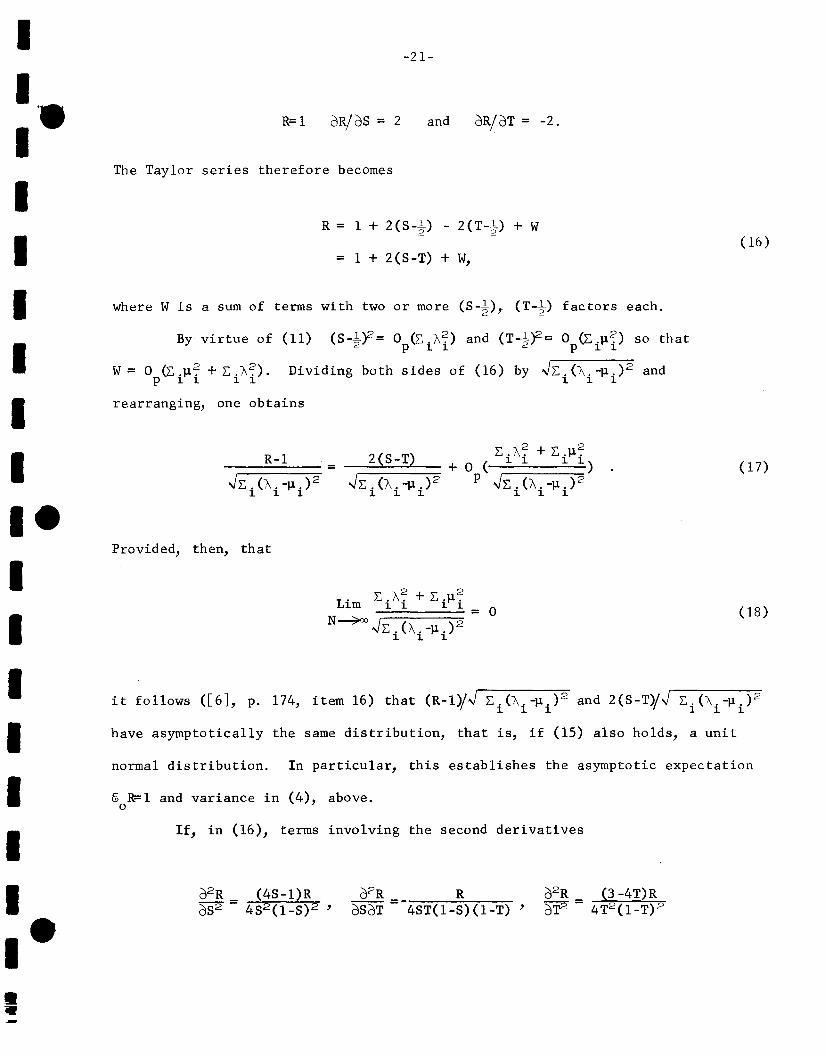
normal distribution. In particular, this establishes the asymptotic expectation

(16)

(18)

(17)

2JR/2JT = -2.and

-21-

2J2 R R2J82JT = -48T(1-8)( l-T) ,

2JR/2J8 = 2R=l

(ll) (8-1.)2= 0 (L, .A~) and (T-l.}2= 0 (L, .).1~) so that2 p ~ ~ 2 P ~ ~

Dividing both sides of (16) by Jr..("\.-).1.)2 and~ ~ ~

R = 1 + 2 (8 -t) - 2 ( T-t) + w

= 1 + 2(8-T) + W,

R-l 2(8-T) r..A::' +r..).1::'-;=======;: = --::===::;::; + 0 ( ~ ~ ~ ~)Jr. . (A. _).1.)2 Jr. . (A. _).1.)2 P Jr.. (A. _).1.)2

~ ~ ~ ~ ~ ~ ~ ~ ~

If, in (16), terms involving the second derivatives

W = 0 (L, .).1::' + r. .A~).p ~ ~ ~ ~

The Taylor series therefore becomes

By virtue of

where W is a sum of terms with two or more (S-t), (T-t) factors each.

rearranging, one obtains

/j; R=l and variance in (4)" above.o

it follows ([6], p. 174, item 16) that (R-l)/.j r..(A.-).1.)2 and 2(8-T)/J r..("\.-).1.)2/ ~ ~ ~ / ~ ~ ~

have asymptotically the same distribution, that is, if (15) also holds, a unit

Provided, then, that

II.-IIIIIII_IIIIIII eI•:w

-22 -

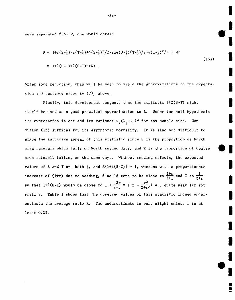
were separated from W, one would obtain

( l6a)

= 1+2 (8-T)+2 (8-T)2+WI .

After some reduction, this will be seen to yield the approximations to the expecta-

tion and variance given in (7), above.

Finally, this development suggests that the statistic 1+2(8-T) might

itself be used as a good practical approximation to R. Under the null hypothesis

its expectation is one and its variance ~.(A.-~.)2 for any sample size. Con­~ ~ ~

dition (15) suffices for its asymptotic normality. It is also not difficult to

argue the intuitive appeal of this statistic since 8 is the proportion of North

area rainfall which falls on North seeded days, and T is the proportion of Centre

area rainfall falling on the same days. Without seeding effects, the expected

values of Sand T are both~, and ~{1+2(8-T)} = 1, whereas with a proportionate

l+r 1increase of (l+r) due to seeding, S would tend to be close to 2+r and T to 2+r

2r r 2so that l+2(S-T) would be close to 1 + 2-+r = l+r - 2+r,i.e., quite near l+r for

small r. Table 1 shows that the observed values of this statistic indeed under-

estimate the average ratio R. The underestimate is very slight unless r is at

least 0.25.

IIII-.1IIIIIII

_IIIIIIII-•••