e-learning electricity & electronics control & instrumentation … · 2020. 10. 9. ·...

E-Learning

Electricity & Electronics

Control & Instrumentation

Process Control

Mechatronics

Telecommunications

Electrical Power & Machines

Test & Measurement

AntennaLab AntennaLab AntennaLab AntennaLab Student’s Workbook

57-200-USB-0S

Feedback

Feedback Instruments Ltd, Park Road, Crowborough, E. Sussex, TN6 2QR, UK. Telephone: +44 (0) 1892 653322, Fax: +44 (0) 1892 663719.

email: [email protected] website: http://www.fbk.com

Manual: 57-200-USB-0S Ed01 102002 Printed in England by Fl Ltd, Crowborough

Feedback Part No. 1160–57200USB0S

AntennaLabAntennaLabAntennaLabAntennaLab WORKBOOK Preface

57-200-USB-0 i

THE HEALTH AND SAFETY AT WORK ACT 1974

We are required under the Health and Safety at Work Act 1974, to make available to users of this equipment certain information regarding its safe use.

The equipment, when used in normal or prescribed applications within the parameters set for its mechanical and electrical performance, should not cause any danger or hazard to health or safety if normal engineering practices are observed and they are used in accordance with the instructions supplied.

If, in specific cases, circumstances exist in which a potential hazard may be brought about by careless or improper use, these will be pointed out and the necessary precautions emphasised.

While we provide the fullest possible user information relating to the proper use of this equipment, if there is any doubt whatsoever about any aspect, the user should contact the Product Safety Officer at Feedback Instruments Limited, Crowborough.

This equipment should not be used by inexperienced users unless they are under supervision.

We are required by European Directives to indicate on our equipment panels certain areas and warnings that require attention by the user. These have been indicated in the specified way by yellow labels with black printing, the meaning of any labels that may be fixed to the instrument are shown below:

CAUTION - RISK OF DANGER

CAUTION - RISK OF

ELECTRIC SHOCK

CAUTION - ELECTROSTATIC

SENSITIVE DEVICE

Refer to accompanying documents

PRODUCT IMPROVEMENTS We maintain a policy of continuous product improvement by incorporating the latest developments and components into our equipment, even up to the time of dispatch.

All major changes are incorporated into up-dated editions of our manuals and this manual was believed to be correct at the time of printing. However, some product changes which do not affect the instructional capability of the equipment, may not be included until it is necessary to incorporate other significant changes.

COMPONENT REPLACEMENT Where components are of a ‘Safety Critical’ nature, i.e. all components involved with the supply or carrying of voltages at supply potential or higher, these must be replaced with components of equal international safety approval in order to maintain full equipment safety.

In order to maintain compliance with international directives, all replacement components should be identical to those originally supplied.

Any component may be ordered direct from Feedback or its agents by quoting the following information:

1. Equipment type

3. Component reference

2. Component value

4. Equipment serial number

Components can often be replaced by alternatives available locally, however we cannot therefore guarantee continued performance either to published specification or compliance with international standards.

AntennaLabAntennaLabAntennaLabAntennaLab WORKBOOK Preface

57-200-USB-0 ii

DECLARATION CONCERNING ELECTROMAGNETIC COMPATIBILITY Should this equipment be used outside the classroom, laboratory study area or similar such place for which it is designed and sold then Feedback Instruments Ltd hereby states that conformity with the protection requirements of the European Community Electromagnetic Compatibility Directive (89/336/EEC) may be invalidated and could lead to prosecution.

This equipment, when operated in accordance with the supplied documentation, does not cause electromagnetic disturbance outside its immediate electromagnetic environment.

COPYRIGHT NOTICE

© Feedback Instruments Limited

All rights reserved. No part of this publication may be reproduced, stored in a retrieval system, or transmitted, in any form or by any means, electronic, mechanical, photocopying, recording or otherwise, without the prior permission of Feedback Instruments Limited.

ACKNOWLEDGEMENTS Feedback Instruments Ltd acknowledge all trademarks.

IBM, IBM - PC are registered trademarks of International Business Machines.

MICROSOFT, WINDOWS XP, 2000, ME, 98 are registered trademarks of Microsoft Corporation.

.

AntennaLab AntennaLab AntennaLab AntennaLab WORKBOOK Contents

57-200-USB-0 TOC 1

TABLE OF CONTENTS

CHAPTER 1 1-1

Introduction

CHAPTER 2 2-1

Assignment 1 Familiarisation 2-1-1

Assignment 2 The Dipole in Free Space 2-2-1

Assignment 3 Effects of the Surroundings 2-3-1

Assignment 4 Dual Sources 2-4-1

Assignment 5 Gain, Directivity and Aperture 2-5-1

Assignment 6 Ground reflections 2-6-1

Assignment 7 The Monopole 2-7-1

Assignment 8 Phased Monopoles 2-8-1

Assignment 9 Resonance, Impedance and Standing Waves 2-9-1

Assignment 10 Return Loss and VSWR Measurements 2-10-1

Assignment 11 Parasitic Elements 2-11-1

Assignment 12 Multi-Element Parasitic Arrays 2-12-1

Assignment 13 Stacked and Bayed Arrays 2-13-1

Assignment 14 The Horn Antenna 2-14-1

Assignment 15 The Log Periodic Antenna 2-15-1

Assignment 16 The Dish Antenna 2-16-1

AntennaLab AntennaLab AntennaLab AntennaLab WORKBOOK Contents

57-200-USB-0 TOC 2

Notes

Chapter 1 AntennaLabAntennaLabAntennaLabAntennaLab WORKBOOK Introduction

57-200-USB-0 1-1

INTRODUCTION

AntennaLab comprises hardware, software and courseware, which together form an integrated learning environment for the study of antenna principles.

Understanding antennas is often thought of as a ‘black art’. The theoretical study of antennas can be mathematically demanding, requiring knowledge of electric field theory, spherical geometry, calculus and other advanced mathematical concepts. However, even armed with these mathematical tools, analysing the performance of antennas in real, practical situations relies heavily on experience, as it is very difficult to include all of the vagueries of an antenna’s electrical and physical surroundings in theoretical calculations.

Don’t worry! The work done with AntennaLab is essentially non-mathematical in its approach to the subject. The practical aspects and effects associated with antennas are stressed and the software that is supplied with AntennaLab takes care of the high-level mathematics. The unique blend of hardware and software experimentation described in this manual leads to a practical understanding of antenna performance that would be difficult to achieve with either hardware or software alone.

Required Equipment

The following items of equipment, software and documentation are required to use the system.

• AntennaLab hardware as described in the Operator’s Manual.

• Discovery Software

• NEC-Win Software

• Operator’s Manual

• This Manual

• The ARRL Antenna Book

• Antenna Theory, Analysis & Design (Constantine A. Balanis)

Chapter 1 AntennaLabAntennaLabAntennaLabAntennaLab WORKBOOK Introduction

57-200-USB-0 1-2

Pre-requisite Knowledge

To be able to understand the assignment work covered by AntennaLab, it is assumed that you have a general basic knowledge of electrical circuit theory. Also, an understanding of the concepts of direct and alternating current and voltage, frequency, amplitude and phase, resistance, impedance and resonance is required.

Some knowledge, or experience, of radio and high frequency techniques will be useful, though not essential, for understanding the work covered by AntennaLab.

Modelling and Simulation

The assignment work throughout this manual uses the two techniques of hardware modelling and software simulation to help explain the principles of how antennas perform. Each of these techniques has its advantages and disadvantages, with one being better for some purposes, the other for others.

As you progress through the assignments, these strengths and weaknesses will be explained and you will appreciate how both the hardware and software tools can be used to give a good understanding of antenna operation.

Obviously, the assignment work in this manual cannot cover the whole of antenna theory and practice. It merely gives a firm basis for further study. Both the hardware and software of AntennaLab are capable of use for more advanced work, or for professional purposes. Their limitations are your imagination!

Chapter 2 AntennaLabAntennaLabAntennaLabAntennaLab WORKBOOK Assignments

57-200-USB-0 2-1

ASSIGNMENTS

Assignment Contents

The Assignment work covered in this manual is as follows:

Assignment 1 Familiarisation

Assignment 2 The Dipole in Free Space

Assignment 3 Effects of the Surroundings

Assignment 4 Dual Sources

Assignment 5 Gain, Directivity and Aperture

Assignment 6 Ground reflections

Assignment 7 The Monopole

Assignment 8 Phased Monopoles

Assignment 9 Resonance, Impedance and Standing Waves

Assignment 10 Return Loss and VSWR Measurements

Assignment 11 Parasitic Elements

Assignment 12 Multi-Element Parasitic Arrays

Assignment 13 Stacked and Bayed Arrays

Assignment 14 The Horn Antenna

Assignment 15 The Log Periodic Antenna

Assignment 16 The Dish Antenna

Chapter 2 AntennaLabAntennaLabAntennaLabAntennaLab WORKBOOK Assignments

57-200-USB-0 2-2

Notes

Chapter 2 AntennaLabAntennaLabAntennaLabAntennaLab WORKBOOK Assignment 1

57-200-USB-0 2-1-1

ASSIGNMENT 1. FAMILIARISATION

Objectives

When you have completed this assignment you will:

• be familiar with the basic operation of the AntennaLab hardware and the Discovery measurement software,

• be familiar with the basic operation of NEC-Win antenna modelling software.

Knowledge Level

As noted in the Introduction.

Preliminary Procedure

Before you start you should have:

• connected up the hardware of AntennaLab as described in the Operator’s Manual,

• loaded the Discovery software as described in the Operator’s Manual,

• loaded the NEC-Win software as described in its accompanying manual,

• read the Using AntennaLab chapter in the Operator’s Manual.


57-200-USB-0 2-1-2

Practical 1.1 Hardware Familiarisation

Getting the System going

Ensure that the AntennaLab hardware is switched off.

Read and refer to the equipment list in the Operator’s Manual to ensure that you can identify the component parts of the Trainer.

Mount one of the Yagi boom assemblies onto the top of the Generator Tower, using two of the screws provided.

Ensure that all the elements of this antenna are removed, except for the dipole element.

Position the dipole element centrally between the boom fixing points to the Generator Tower.

Ensure that the Motor Enable switch on the rear panel of the Generator Tower is off and then run the Discovery software and navigate to the AntennaLab section.

WARNING

If the system is left switched on but unattended, the Motor Enable switch must be switched OFF. This is because power line fluctuations may cause the motor to rotate the antenna continuously and damage the coaxial cable. Also, do not leave the hardware switched on with the computer off as this also may cause the antenna to rotate continuously.


57-200-USB-0 2-1-3

Setting the antenna

Navigate to the Signal Strength vs. Angle application page. Select the 2D polar graph window and immediately switch on the Motor Enable switch.

When the window appears, the software will then set the motor to its index position, which involves rotating the test antenna through up to 180 degrees from its initial position.

The antenna must now be set to line up with the receiver.

Set the distance between the Receiver and Generator Towers to be about one metre.

Loosen the knurled screw located at the bottom of the white nylon part of the Receiver Tower and turn the receiving antenna (the four log periodics) to point directly at the Generator Tower. Tighten the knurled screw.

Repeat this procedure for the Generator antenna, ensuring that the boom of the antenna is pointing directly at the Receiver.

Ensure that the coaxial cables that protrude from the grey parts of the Receiver and Generator Towers are connected to their relevant antennas.

Read the Instructions!

Instructions on how to use the system are given in the software.

Each application section provides information as does the help section. In the Discovery tree, select ‘Help’ then ‘Using AntennaLab’. Read these in turn. You may not understand all that you read – but things will become clearer as you use the system.


57-200-USB-0 2-1-4

The Application Node

In the Discovery tree, navigate to ‘Application’ then ‘Signal Strength vs. Frequency’. Select the frequency graph window.

A graph window will appear on the screen. From the menu select ‘File’ then ‘New Plot’.

A plot of received signal vs. frequency is made similar to that shown in Figure 2-1-2. What the hardware is doing is stepping through the frequency range, from 1200 MHz to 1800 MHz, in small steps and automatically recording and plotting the signal that is received. You can see how fast it does it compared to taking individual measurements – and how little effort you have to use!

Figure 2-1-2: A Typical Frequency Plot

Now, in the Discovery tree, navigate to ‘Signal Strength vs. Angle’ and select the 2D polar graph window. From the menu select ‘File’ then ‘New Plot’. A dialogue box will appear allowing you to enter a frequency. Click ‘OK’ to accept 1500 MHz (in the middle of the available range).


57-200-USB-0 2-1-5

The motor will start, the antenna will first move to find its reference point and then rotate through 360°. The antenna response will then be plotted as shown in Figure 2-1-3. The significance of this plot will become apparent later. The motor then returns to its reference position.

Figure 2-1-3: A Typical Polar Plot

The polar plotting routine that you have just been through only took a few seconds. The equipment was automatically taking readings every degree, as it rotated. Again, you can see how quick and easy it is to do these measurements!


57-200-USB-0 2-1-6

Now, navigate to ‘Monitor’, and select the signal strength monitor. Again, the default frequency is 1500 MHz. A bar-graph will appear as shown in Figure 2-1-4.

Figure 2-1-4: The Bar-Graph Display

Wave your hand about in the space between the Generator and the Receiver antennas. The bar-graph will go up and down. This gives another form of indication of the received signal.

Other AntennaLab features will be dealt with at a later stage.


57-200-USB-0 2-1-7

Practical 1.2 NEC-Win Software Familiarisation

Ensure that you have read the introductory sections in the NEC-Win manual.

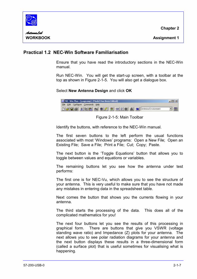
Run NEC-Win. You will get the start-up screen, with a toolbar at the top as shown in Figure 2-1-5. You will also get a dialogue box.

Select New Antenna Design and click OK

Figure 2-1-5: Main Toolbar

Identify the buttons, with reference to the NEC-Win manual.

The first seven buttons to the left perform the usual functions associated with most ‘Windows’ programs: Open a New File; Open an Existing File; Save a File; Print a File; Cut; Copy; Paste.

The next button is the ‘Toggle Equations’ button that allows you to toggle between values and equations or variables.

The remaining buttons let you see how the antenna under test performs:

The first one is for NEC-Vu, which allows you to see the structure of your antenna. This is very useful to make sure that you have not made any mistakes in entering data in the spreadsheet table.

Next comes the button that shows you the currents flowing in your antenna.

The third starts the processing of the data. This does all of the complicated mathematics for you!

The next four buttons let you see the results of this processing in graphical form. There are buttons that give you VSWR (voltage standing wave ratio) and Impedance (Z) plots for your antenna. The next allows you to see polar radiation diagrams for your antenna and the next button displays these results in a three-dimensional form (called a surface plot) that is useful sometimes for visualising what is happening.


57-200-USB-0 2-1-8

The final button launches NEC-Vu 3D for visualising complex, 3D antenna models.

You will get to know how these, and the other buttons on the toolbar, work as you progress through the assignments.

Below the main toolbar there is an area like a spreadsheet. This is the area in which you tell the program the dimensions of the antenna that you want to investigate.

Figure 2-1-6: Antenna Dimension Screen

This is the screen that you will use most when specifying antennas for investigation. You will soon get to know how to use it.


57-200-USB-0 2-1-9

An Example File

Click on the Open File button on the toolbar and then open Yagi.

You will see that numbers have appeared in the table. These are the details of this particular antenna. Don’t worry about what they mean, at this stage.

To see what the antenna looks like, click on the NECVu button (the one with the eye on it).

Figure 2-1-7: A NECVu Screen

Use the scroll bars to see how the structure rotates to give you different views.

Try using the buttons down the right side of the screen to see what each does.

When you are satisfied that you know what happens, quit NECVu.


57-200-USB-0 2-1-10

Processing and Results

Click on the ‘Run NEC’ button (the one with the traffic light). A dialogue box should tell you that that your PC is processing the data.

When the processing is complete, press any key to continue. Click on the ‘Polar Plot’ button (with the rose-like icon). A box will appear with ‘Elevation’ selected in the ‘Available Patterns’ table.

Click ‘ Generate Graph’.

A plot of the antenna’s performance should appear similar to that shown in Figure 2-1-8. At this stage, you will not necessarily know what this means – be patient!

Figure 2-1-8: The Antenna’s Plot

Click the left mouse button anywhere on the screen and then ‘Exit Plots’ in the box, to get back to the main table.


57-200-USB-0 2-1-11

Lastly, click on the ‘Surface’ button (the next right on the toolbar). A dialogue box will appear. Click on ‘Process’ and wait. It might take some time to do all of the computations but, eventually, you will get a surface plot of the antenna’s performance similar to that shown in Figure 2-1-9.

Figure 2-1-9: A Surface Plot

You can use your mouse and the keyboard to investigate this plot – in a similar way to that for NECVu.

When you have finished, close the Surface Plot window.

You have now seen how NEC-Win processes and shows the results. NEC-Win has more features. You will see them all as you progress.


57-200-USB-0 2-1-12

Notes


57-200-USB-0 2-2-1

ASSIGNMENT 2. THE DIPOLE IN FREE SPACE

Objectives


• have learnt how to describe an antenna in NEC-Win,

• have investigated the polar plots of a dipole in free space with both software simulation and hardware modelling,

• have compared the results of both methods.

Knowledge Level

You should have performed Assignment 1.








57-200-USB-0 2-2-2

Introduction

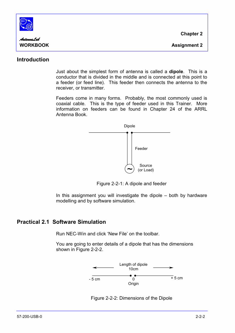
Just about the simplest form of antenna is called a dipole. This is a conductor that is divided in the middle and is connected at this point to a feeder (or feed line). This feeder then connects the antenna to the receiver, or transmitter.

Feeders come in many forms. Probably, the most commonly used is coaxial cable. This is the type of feeder used in this Trainer. More information on feeders can be found in Chapter 24 of the ARRL Antenna Book.

Figure 2-2-1: A dipole and feeder

In this assignment you will investigate the dipole – both by hardware modelling and by software simulation.

Practical 2.1 Software Simulation

Run NEC-Win and click ‘New File’ on the toolbar.

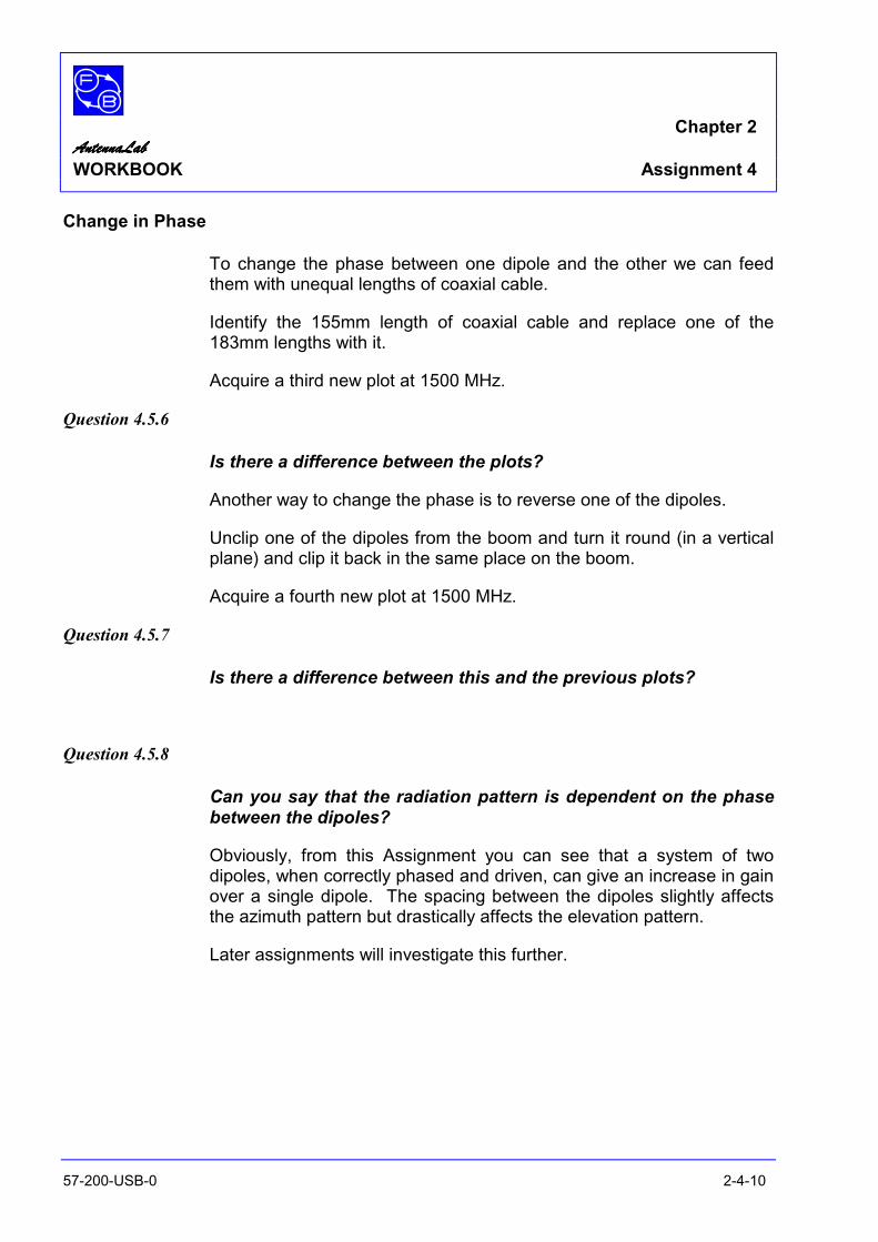
You are going to enter details of a dipole that has the dimensions shown in Figure 2-2-2.

Figure 2-2-2: Dimensions of the Dipole

Dipole

Feeder

~ Source(or Load)

Length of dipole 10cm

0 Origin

+ 5 cm - 5 cm


57-200-USB-0 2-2-3

Setting Up the Dipole Dimensions

The table requires dimensions in all of the three directions. The ‘y’ direction we will take as being along the direction of the wire of the dipole, the ‘x’ direction will be at right-angles to this, but on the same horizontal plane, and the ‘z’ direction at right-angles in a vertical plane.

Figure 2-2-3: The Three Axes

We want the centre of the dipole at the origin of the axes. This means that the two ends will be at +y and –y, where y is half of the total length of the dipole. The dipole we want is to have a total length of 10cm, i.e. ±5cm.

Firstly, enter the figure –0.05 (for 5cm – the dimensions are in metres) in the table under ‘Y1’ for Wire 1. This is the x co-ordinate of one end of the dipole. To do this, move the cursor onto the required cell of the table and click the left mouse button. A box appears round the cell, with a highlighted ‘0’ in it. Just type -0.05. Don’t forget the minus sign!

When you press the Enter key, the –0.05 is entered into the Y1 cell and the box moves along to the next cell.


57-200-USB-0 2-2-4

The dipole does not have any dimension in the X, or Z directions, so the X1 and Z1 co-ordinates should be zero. Just press the Enter key to accept zeros for these cells.

The y co-ordinate of the other end of the dipole is +0.05. Enter this in in the Y2 cell – you don’t actually have to type in the plus sign, as the software assumes all non-minus figures to be plus.

Click the mouse on the ‘Dia.’ Cell on the Wire 1 row. A dialogue box appears. Select the ‘Other’ box at the bottom and enter 0.004 (a diameter of 4mm). Click ‘OK’.

Setting Up the Segments

In the cell under ‘Seg’, enter 9. This determines the number of segments the wire is divided into for computation. The higher the number you put in here, the more accurate the results will be – but the longer the calculations will take to perform. For a simple antenna like a dipole, 9 is a good compromise. Note that it is always better to choose an odd number.

Setting Up the Source

Click on the cell under ‘Src/Ld’. A box comes up with a picture of the wire, split up into its segments. You need to put a source (of signal) in the middle of it – because this is where the dipole is being fed. Now you can see why it is best to choose an odd number of segments, so that there is a middle one!

Use your mouse to ‘drag and drop’ a Source (the green square symbol with a sinewave on) onto the middle section of the wire (between points 5 and 6).

Another box will appear. Just press OK to accept these settings for the source. Press ok on the main box to accept the source as a whole. The figures ‘1/0’ will appear in the cell, if you have done things correctly.

Setting the Wire Conductivity

If you click on the cell under ‘Conduct’ a box appears that will let you specify the type of conductor that the wire is made of. We will stick with a perfect conductor for this example. Just click OK.


57-200-USB-0 2-2-5

Setting the Frequency

We will be comparing the results obtained from the simulation with those from the hardware modelling, so it is sensible to use the same frequency for both: 1500 MHz.

Figure 2-2-4: The Frequency box

Observe the ‘Frequency [MHz]’ box, just below the tool bar.

Enter 1500 in the ‘Start’ box. Enter 1500 in the ‘End’ box and 0 in the ‘Step Size’ box.

Make sure ‘Linear Stepping’ is selected and then click OK.

Setting the Output Requirements

We will use the default output settings for this practical, so no changes need to be made.

NECVu

Use NECVu to visualise the antenna that you have just entered. The two end segments should be blue and the rest of the dipole should be red. If you do not have this, then you have made a mistake in entering the dimensions. Check them!

Process the Data

Click on the Run NEC button (traffic lights). A box asks what you want to call the file and where to save it. Probably, it is better to set up a directory of your own in which to store your results, rather than use the NEC-win\examples directory. If you do not know how to do this, ask your instructor.

We suggest you call the file: dipole1

NEC-Win will now do the processing.


57-200-USB-0 2-2-6

Looking at the Results

Click on the Polar Plot button. You will see that the ‘Elevation Plot’ is highlighted. Click on the little box to the left of ‘Elevation Plot’ to de-select this plot and click on the little box to the left of ‘Azimuth Plot’ to select it. This gives the plot of the antenna in the horizontal plane (the x-y plane). Now click on the Generate Graph button.

An azimuth polar plot of the antenna pattern will appear.

The distance of the line from the centre of the circle indicates the relative amount of power that the antenna will receive or transmit in each particular direction.

Figure 2-2-4: A Typical Azimuth Plot

Question 2.1.1

Does the dipole antenna have the same response in all directions in the azimuth (horizontal) plane?

Question 2.1.2

In which direction(s) is the response a maximum?

Question 2.1.3

In which direction(s) is the response a minimum?

Elevation Plot

Move the cursor to anywhere on the scaled part of the polar plot and click the left mouse button. The Azimuth Plot Control box will appear.


57-200-USB-0 2-2-7

Click on Select and then select the Elevation plot by clicking on the little box to the left of ‘Elevation’ in the table. The highlighted box should move down to Elevation. De-select the Azimuth plot by clicking on the box to the left of ‘Azimuth’ in the table.

Click Generate Graph.

Figure 2-2-5: The Elevation Plot

Question 2.1.4

Does the dipole antenna have the same response in all directions in the elevation (vertical) plane?

Question 2.1.5

In which direction(s) is the response a maximum?

Question 2.1.6

In which direction(s) is the response a minimum?

Move the cursor to anywhere on the scaled part of the polar plot and click the left mouse button. The Elevation Plot Control box will appear. Click on Exit Plots

Surface Plot

Display a surface plot of the antenna response by clicking on the Surface button, then Continue.


57-200-USB-0 2-2-8

Question 2.1.7

Does the surface plot agree in shape with your polar plots?

Note that you have only plotted half of the elevation plot: with θ from 0° to 90°. The other half will just be a continuation of the pattern that you have obtained.

We could change the surface plotting parameters to get a full plot, but this would mean that a huge amount of calculation would have to be done by the computer. This would take a long time and, unless you have a very large amount of memory in your PC, there would probably be so much data for it to handle that the program might crash.

As a full plot is unnecessary, we won’t bother to try!

Practical 2.2 Hardware Modelling

Set up the AntennaLab hardware as detailed before.

Ensure that the antenna mounted on the Generator Tower is a single dipole, only.

Examine the dipole element. You will see that the ends of the dipole are extendible. Adjust the dipole length so that it is 5cm either side of the centre.

Ensure that the Motor Enable switch is off and then switch on the Trainer.

Run the Discovery AntennaLab software.

Ensure that the Receiver and Generator antennas are aligned with each other and that the spacing between them is about one metre.

Select the signal strength vs. angle 2D graph and immediately switch on the Motor Enable switch. Acquire a new plot at a frequency of 1500 MHz. The Trainer will plot the polar response of your dipole at this frequency.


57-200-USB-0 2-2-9

Question 2.2.1

How does this plot compare with the azimuth plot you obtained with NEC-Win in Practical 2.1?

Question 2.2.2

Is it exactly the same shape, roughly the same shape, or nothing like the same shape?

Simulation and Reality

You have now achieved plots for your 10cm-long dipole at 1500MHz using both NEC-Win software for simulation and the AntennaLab’’s hardware for modelling.

Remember, simulation gives the performance of the antenna using a mathematical model of the system. The maths is complex, but the software and the PC do the hard work for you. The results that you get from a simulation depend directly on the accuracy of that mathematical model. This means that, ideally, the model should take into account everything about that antenna and its surroundings.

Question 2.2.3

Did you enter any details about any of the surroundings into NEC-Win?

So far, the way you have been using NEC-Win has assumed that there are no surroundings! The only way that it would be possible to get a real antenna into a situation with no surroundings is if it was many km away from the Earth in outer space.

For this reason, when no consideration is taken of the surroundings, the dipole is referred to as ‘in free space’.

What about the hardware modelling of the dipole that you have just done?


57-200-USB-0 2-2-10

Question 2.2.4

Was the dipole mounted on the Generator Tower being operated in ‘free space’?

The results that you get from hardware modelling using AntennaLab reflect the fact that it is being used in a real-world environment – not in free space.

The surroundings of the laboratory are all automatically being taken into account when you do measurements with the hardware.

The sorts of patterns that you get from software simulation are, usually, ideal. Those that you get from hardware modelling are ‘the real thing’.

You will see, as you progress through the assignments, that the combination of both techniques is very powerful and leads to a greater understanding of antenna principles and performance than either used on its own.


57-200-USB-0 2-2-11

Figure 2-2-6: Software Simulation Plot

Figure 2-2-7: Hardware plot shows effects of environment


57-200-USB-0 2-2-12

Notes


57-200-USB-0 2-3-1

ASSIGNMENT 3 EFFECTS OF THE SURROUNDINGS

Objectives


• have investigated how the physical surroundings effect the performance of an antenna.

Knowledge Level









57-200-USB-0 2-3-2

Introduction

In Assignment 2, you have seen how both software simulation and hardware modelling may be used to find out how an antenna performs.

The results that are obtained from each of these methods are similar, but not exactly the same. This was stated to be because the software simulation in Assignment 2 was assuming free space, whereas the hardware modelling was done in the ‘real world’.

In this Assignment you will look in more detail at the hardware modelling to see that changes in surroundings do give changes in antenna performance.

Practical 3.1 Absorption and Reflection

Setting up the Practical

The set up of the AntennaLab hardware is the same as for Assignment 2, Practical 2.2.

Ensure that the antenna mounted on the Generator Tower is a single dipole, only.

Adjust the dipole length so that it is 5cm either side of the centre.


The Signal Level Bargraph

Select the signal strength monitor.

A bargraph will appear on the screen. Don’t worry about what the figures mean, you will learn about these later.


57-200-USB-0 2-3-3

The bargraph is a measure of the signal power received by the antenna on the Receiver Tower from the antenna on the Generator Tower. If more signal is received, the bar will rise, if less, it will fall.

Figure 2-3-1: The Bargraph Display


57-200-USB-0 2-3-4

Move your hand in between the two antennas.

Question 3.1.1

Does the level of the bar change?

Identify the Ground Plane that comes with AntennaLab. It is an aluminium sheet with some holes in it.

Hold the Ground Plane in between the two antennas.

Question 3.1.2


Question 3.1.3

Does it change more, or less than with your hand?

Obviously, the amount of signal reaching the receiver is dependent on what is between its antenna and the generator antenna.

Let us see what happens when something is placed near to the side of the antenna.

Move your hand about at the side of the dipole.


57-200-USB-0 2-3-5

Question 3.1.4


Hold the Ground Plane at the side of the dipole.

Question 3.1.5


You should see that the changes are much less, if at all, for surrounding objects to the side of the antenna. This would seem reasonable, if you remember the azimuth plots that you obtained in Assignment 2, as there is very little response to the side of a dipole.

Hold the Ground Plane close to the end of the boom on which the dipole is mounted. Note the level of the bargraph. Now, slowly move the Ground Plane away from the dipole, keeping it in line between the two antennas.

Question 3.1.6

How does the bar vary?

Question 3.1.7

Can you think of a reason for the way that it varies?

Don’t worry if you cannot. This will be explained in a later assignment.

Polar Plots

Select the signal strength vs. angle 2D graph. Acquire a new plot at a frequency of 1500 MHz.

A polar plot will be taken and displayed.

Now, hold up the Ground Plane level with the dipole but to one side and angled towards the Receiver.

Acquire a second new plot also at 1500 MHz.

A second polar plot will be superimposed over the first.


57-200-USB-0 2-3-6

Question 3.1.8

Are the two patterns the same?

Obviously, the sheet of aluminium has an effect on the way that the signal gets from the Generator to the Receiver. When put between the Generator and Receiver antennas, the sheet reflects some of the radiating signal.

Now, in a practical situation, there is unlikely to be a large sheet of metal in close proximity to the antenna – but there could be a water tank, a building, or some trees. All of these will have an effect on the performance of the antenna, how well it radiates, or receives.

The surroundings of an antenna are an important factor. Very often experimenting on antennas is performed well away from other objects – perhaps in the middle of an open space, or in a special room that has been constructed so that electromagnetic waves are absorbed by its walls (an anechoic chamber). You are probably doing your experimentation with AntennaLab in a laboratory. There will be other things close-by that affect the performance. But a situation like that is the ‘real world’ and it is important for you to realise that antennas are operated in the real world and will be affected by their surroundings.


57-200-USB-0 2-4-1

ASSIGNMENT 4 DUAL SOURCES

Objectives


• have seen how a system of two dipoles performs in comparison with a single dipole,

• how the spacing between the dipoles affects the performance,

• how the magnitude of the drive signal to each dipole affects the performance,

• how the phase difference between the two dipoles affects the performance.

Knowledge Level









57-200-USB-0 2-4-2

Introduction

From Assignment 3, you will have noticed the effects of reflections of signal from surrounding objects. When the aluminium sheet was used, the situation was as shown in Figure 2-4-1, below.

Figure 2-4-1: Reflection

Notice that there is a ‘virtual’ source dipole due to the reflection effect.

In this assignment you will investigate what happens when you have two source dipoles and we will compare the effects to those found in Assignment 3.

Practical 4.1 Software Simulation of Two Dipoles

Run NEC-Win and click Open File on the toolbar. Open the file you used for Assignment 2 (dipole1).

Ensure that you have no ground set and that the frequency is set to 1500MHz.

Click on the Run NEC button and then examine the azimuth and elevation plots produced.

Copy the Wire1 line into the Wire 2 line.

Click on Z1 for Wire 2 and change it to 0.5. Also change Z2 for Wire 2 to 0.5.

You have now set up two dipoles at a vertical distance of 0.5m apart.

Save this as 2dipole.

Dipole Under Test

Virtual Dipole Metal

SheetReceiving Antennas


57-200-USB-0 2-4-3

Ensure that you have no ground set and that the frequency is set to 1500 MHz.

Click on the Run NEC button.

Examine the azimuth and elevation plots produced.

Comparing the Single and Two Dipole Plots

NEC-Win allows you to plot the responses of different antennas on the same graph for comparison.

From the ‘Radiation Pattern Select/Configure’ window, click on Add File. Select the file dipole1.nou when prompted. You will then get the window shown in Figure 2-4-2.

Figure 2-4-2: Radiation Pattern Select Window

In this window, select Azimuth for DIPOLE1 (do not de-select Azimuth for 2DIPOLE). Now, you have both antenna azimuth plots selected. To make them different colours, click on ‘Line Type’ in the ‘Total Gain’ box and change this to the continuous line, click on ‘Line Color’ and change this to red, then click on ‘’Line Width’ and choose one of the wider lines.

Then click Generate Graph and you will get a plot of the two antennas, with the single dipole in red and the two-dipole combination in blue.


57-200-USB-0 2-4-4

Question 4.1.1

Is there a difference between the two plots?

Go through a similar procedure to display the elevation plots for the antennas. You should end up with patterns like Figure 2-4-3.

Figure 2-4-3: Azimuth and Elevation Patterns

Go back to the main NEC-Win window for 2DIPOLE (the input table) and click on the Surface Plot button to examine the surface plot of the two-dipole combination.

Practical 4.2 Changing the Dipole Spacing

Let us now change the spacing between the dipoles.

Ensure that you are in the main NEC-Win window for 2DIPOLE and change the figures for Z1 and Z2 in Wire 2 to 0.1.

Repeat the procedure for Practical 4.1 and see what happens.

Question 4.2.1

Are your results the same as for Practical 4.1?

Repeat for other spacings between the dipoles.


57-200-USB-0 2-4-5

Question 4.2.2

Can you say that the radiation pattern is dependent on the spacing between the dipoles?

Practical 4.3 Changing the Magnitude of the Source

Ensure that you are in the main NEC-Win window for 2DIPOLE and the figures for Z1 and Z2 in Wire 2 are 0.5.

Click File and then Save on the menu bar at the top.

Click on the Src/Ld box for Wire 2.

Click on the green source icon between points 5 and 6 on the dipole (be sure not to move the source icon as you do this). A dialogue box, as shown in Figure 2-4-4 will appear.

Figure 2-4-4: Source Parameters Set-up Dialogue Box

This box allows you to change the parameters of the source. You have been working with nominal sources that have voltages of 1 volt. You can change the voltage of one of the sources and see if that has an effect on the plots.

Change the Magnitude box of this source to 2.0V. Click OK and then OK, again.

Click on the Run NEC button and then examine the plots.


57-200-USB-0 2-4-6

Question 4.3.1

Has changing the magnitude of one of the sources made any difference to the pattern?

Question 4.3.2

Does the azimuth, or the elevation plot change the most?

Repeat for other source voltages.

Question 4.3.3

Can you say that the radiation pattern is dependent on the source voltages of the dipoles?

Practical 4.4 Changing the Phase of the Source

Click on the Src/Ld box for Wire 2.

Click on the green source icon between points 5 and 6 on the dipole (be sure not to move the source icon as you do this). A dialogue box, as shown in Figure 2-4- 5 will appear.

Figure 2-4- 5: Source Parameters Set-up Dialogue Box

Change the Magnitude box of this source back to 1.0V.

Change the Phase box of this source to 90. Click OK and then OK, again.

Click on the Run NEC button and then examine the plots.

Repeat for other source phases.


57-200-USB-0 2-4-7

Question 4.4.1

Can you say that the radiation pattern is dependent on the source phases of the dipoles?

Practical 4.5 Hardware Modelling with Two Dipoles

Setting Up the Hardware

Remove the Yagi Boom assembly from the Generator Tower.

Identify the Yagi Stack base Assembly. It is the thinner of the two grey plastic strips with holes in them. Screw this vertically to the side of the Generator Tower and mount a Yagi Boom assembly to this strip, four holes below the fixing, with the dipole mounted on the boom just forward of the grey plastic strip, as shown in Figure 2-4-6.

Figure 2-4-6: Dipole Stacking



57-200-USB-0 2-4-8

Azimuth Plots

Start the AntennaLab software and select signal strength vs. angle 2D graph. Acquire a new plot at a frequency of 1500 MHz.


Mount the second Yagi Boom assembly to this strip, four holes above the fixing.

Adjust the position and length of the dipole on this second boom to be identical to the first dipole.

Identify the 2-way Combiner. This is a small, green printed circuit with three coaxial sockets mounted on it.

Identify the two 183mm lengths of coaxial cable. Make sure that you have chosen two identical lengths.

Connect these two cables, one to each of the connectors that are close to each other on the 2-way Combiner. Connect the other ends of these cables each to a dipole.

Connect the coaxial cable that comes from the Generator Tower to the third connector on the Combiner.

Acquire a second new plot also at 1500 MHz.

Question 4.5.1


Remove the top dipole from its boom, turn it through 180° and replace it in the same position on the boom.

Acquire a third new plot at 1500 MHz.

Question 4.5.2

Is there a difference between this and the first two plots?

Change the spacing distance between the two dipoles and acquire a fourth new plot at 1500 MHz.

Question 4.5.3


Change the spacing distance between the two dipoles back to four holes either side of the fixing.


57-200-USB-0 2-4-9

Elevation Plots

Because the motor only rotates in one plane, to get an elevation plot with the AntennaLab hardware, the dipoles must be mounted at right-angles to normal. This is shown in Figure 2-4-7.

Figure 2-4-7: Dipoles for Elevation Plot

Also, the Receiver antenna must be changed to the vertical plane. Loosen the knurled screw that is situated in the centre of the four antennas and turn the antennas through 90°.

Open a new signal strength vs. angle 2D graph and acquire a new plot at 1500 MHz.

Change the spacing distance between the two dipoles.

Acquire a second new plot at 1500 MHz.

Question 4.5.4


Question 4.5.5



57-200-USB-0 2-4-10

Change in Phase

To change the phase between one dipole and the other we can feed them with unequal lengths of coaxial cable.

Identify the 155mm length of coaxial cable and replace one of the 183mm lengths with it.


Question 4.5.6

Is there a difference between the plots?

Another way to change the phase is to reverse one of the dipoles.

Unclip one of the dipoles from the boom and turn it round (in a vertical plane) and clip it back in the same place on the boom.

Acquire a fourth new plot at 1500 MHz.

Question 4.5.7

Is there a difference between this and the previous plots?

Question 4.5.8

Can you say that the radiation pattern is dependent on the phase between the dipoles?

Obviously, from this Assignment you can see that a system of two dipoles, when correctly phased and driven, can give an increase in gain over a single dipole. The spacing between the dipoles slightly affects the azimuth pattern but drastically affects the elevation pattern.

Later assignments will investigate this further.


57-200-USB-0 2-5-1

ASSIGNMENT 5 GAIN, DIRECTIVITY AND APERTURE

Objectives


• understand the terms ‘isotropic source’, ‘directivity’, ‘gain’ and ‘aperture’ as applied to antennas,

• understand the term ‘range distance’ as applied to antenna measurements.

Knowledge Level








• read the ‘Antenna Measurements’ section of Chapter 27 of the ARRL Antenna Book.


57-200-USB-0 2-5-2

Introduction

So far, the investigations that have been done have been very qualitative. From now on, most of the results that will be taken will have numerical values. Before you can do this we need to define some terms of reference.

We will do this using examples from the NEC-Win software.

Isotropic Source

Imagine that you could have a point source of radiation in free space.

Because it doesn’t have different dimensions in different directions, it is reasonable to assume that this source would radiate equally in all directions. The pattern of radiation would be spherical.

Although, in reality, such a point source cannot exist, it does give us a reference against which practical antennas may be measured.

This type of source is called an Isotropic Source.

This is discussed further in Chapter 2 of the ARRL Antenna Book.

Practical 5.1 Antenna Directivity and Gain

Antenna Directivity

As you have seen in earlier assignments, the practical antennas that you have investigated do not radiate equally in every direction.

Run NEC-Win and click Open File on the toolbar. Open the file you used for Assignment 2 (dipole1.nwb).

Ensure that you have no ground set and that the frequency is set to 1500 MHz.


Question 5.1.1

Does the dipole radiate equally in all directions?


57-200-USB-0 2-5-3

Because it does not, the antenna is said to have Directivity. Power is concentrated in some directions at the expense of others.

Read the section on ‘Directivity and Gain’ in Chapter 2 of the ARRL Antenna Book.

The Directivity is defined as:

D = P/Pav

Where D = directivity;

P = max. power density;

Pav = average power density

Antenna Gain

Antenna Gain is defined as:

G = kD

Where G = gain

D = directivity

k = efficiency

As the efficiency of an antenna system is usually made as high as possible. Normally, D = G, within a few percent.

Gain and Directivity are usually expressed in decibels.

See the ‘Introduction to the Decibel’ in Chapter 2 of the ARRL Antenna Book.

The gain of a real, practical antenna is referred to an isotropic source.

Gain of a Dipole

Look at the azimuth plot for dipole1.

Click on the menu bar on Options and then on Gain Probe.

Put the mouse cursor anywhere inside the plot and click the left button.


57-200-USB-0 2-5-4

The total gain and the angle are displayed in the Gain Probe box.

Question 5.1.2

What is the maximum gain of the dipole, in dB?

Remember, this is with reference to an isotropic source.

The theoretical gain of a dipole in free space over an isotropic source is 2.14dB.

Question 5.1.3

How does your dipole gain compare with the theoretical value?

Question 5.1.4

What is the percentage difference?

The difference should be very small.

Antenna Aperture

Consider an antenna receiving signals from a remote source. The antenna can be thought to ‘capture’ some of the radiation from the source. The effective ‘capture area’ of the antenna will depend on the properties of the antenna – notably its gain.

This ‘capture area’ is known as the aperture of the antenna.

The relationship between gain and aperture is given by:

Gain = 4ππππAe / λλλλ2

Where Ae is the effective aperture of the antenna.

Note that in this equation the gain must not be in decibels.

Question 5.1.5

What is the equivalent gain as a ratio to 2.14dB?

Question 5.1.6

What is the aperture of a dipole (in square metres) at 1500MHz?


57-200-USB-0 2-5-5

Range Distance

To make reasonably accurate measurements on antennas, the distance between the Generator and the Receiver antennas must be great enough that the electromagnetic field from the generator at the receiving antenna should be uniform over its effective aperture.

The larger the aperture (and hence the gain), the further the two antennas must be apart to achieve this.

The distance between the antennas is called the range distance.

For a circular aperture, the relationship for the minimum range distance Smin is:

Smin = 2λλλλG / ππππ2

Where G is the gain of the antenna under test.

Question 5.1.7

What is the minimum range distance for a dipole at 1500MHz?

Question 5.1.8

Is the range distance that we are using greater than this minimum?


57-200-USB-0 2-5-6

Notes


57-200-USB-0 2-6-1

ASSIGNMENT 6 GROUND REFLECTIONS

Objectives


• understand how a dipole over both perfect and real ground performs.

Knowledge Level




• loaded the NEC-Win software as described in its accompanying manual.


57-200-USB-0 2-6-2

Introduction

You have seen, from earlier assignments, how its surroundings can affect the radiation pattern of an antenna. You have also seen that two antennas (dual sources) change the radiation pattern because of the additive and subtractive properties of the waves radiated.

This assignment investigates how ground reflections affect the performance of an antenna.

Practical 6.1 Single Dipole above Perfect Ground

Run NEC-Win and click Open File on the toolbar. Open file dipole1.

Change Z1 and Z2 to 0.025m.

Click on File then Save As dipole2.

In the ‘Ground’ box just below the tool bar, set the ground to Perfect Ground and ensure that the frequency is set to 1500 MHz.


Question 6.1.1

Are the plots different from those with no ground?

(Note: look carefully at the radial scale of the plot – it’s in dB relative to an isotropic source).

Question 6.1.2

Why do you think that the azimuth plot is so small?

Go back to the main NEC-Win table and click the Add button in the Radiation Patterns box. Change the value of Initial Elevation for the azimuth plot from 1° to 30°.

Click on the Run NEC button and then examine the azimuth plot produced. You can select both of the azimuth plots, give each a different colour line and display them superimposed together.

Question 6.1.3

Has the azimuth plot changed?

Try this again for other values of θ.

Click on the Surface button and examine the surface plot.


57-200-USB-0 2-6-3

Question 6.1.4

Does this agree with your azimuth and elevation plots?

Image Antenna

The reflected wave and the incident wave are shown in Figure 2-6-1: Reflected and Incident Waves.

Figure 2-6-1: Reflected and Incident Waves

This gives rise to an ‘image antenna’ situated below ground, as shown.

Read the section on ‘The Effect of Ground in the Far Field’ in Chapter 3 of the ARRL Antenna Book to learn more about this effect.

Practical 6.2 Two Dipoles in Free Space

Run NEC-Win and click Open File on the toolbar. Open file 2dipole.

Ensure that you have no ground set and that the frequency is set to 1500 MHz. Change Z1 and Z2 for Wire 2 to 0.05.



Antenna

‘Virtual’ ImageAntenna

Direct Wave

Reflected Wave

Perfect Ground


57-200-USB-0 2-6-4

Question 6.2.1

Are the plots for the two antenna systems of Practicals 6.1 and 6.2 similar in shape?

Changing the Phase of one of the Dipoles

Let us see what happens when the phase of the source voltage for one of the dipoles is changed.

On the main table for 2dipole.nwb, click on the Src/Ld square of Line2, then click on the green source icon next to segment 5.

In the box marked ‘Phase:’, change the phase of the source to 180 degrees. Click the OKs to accept this.



Question 6.2.2

How do these plots compare in shape with those from Practical 6.1?

Practical 6.3 Comparing the Single and Two Dipole Plots

Run dipole2 again.

Click on the Output button and change the Initial value of Elevation to 50°.

Click on the Run-NEC button and then Save the file.

Run 2dipole again.

Click on the Output button and change the Initial value of Elevation to 50°.

Click on the Run-NEC button and then click on the Pattern Plot button.


57-200-USB-0 2-6-5

To show the responses of the two antenna systems on the same graph, from the ‘Radiation Pattern Select/Configure’ window, click on Add File. Select the file dipole2.nou when prompted

Now, you can choose different colours for plots of the two antenna systems.

Examine the elevation plots first.

Question 6.3.1

Are the two plots similar in shape?

Question 6.3.2

What is the difference between them in dB in the direction of maximum radiation?

Hint: use the Gain Probe to find this out.

Now, examine the azimuth plots.

Question 6.3.3


Question 6.3.4

What is the difference between them in dB in the direction of maximum radiation?

Question 6.3.5

What is the equivalent gain as a ratio to 3dB?

Question 6.3.6

Can you suggest a reason why the system with two dipoles gives this more gain than the single dipole above perfect ground?


57-200-USB-0 2-6-6

Practical 6.4 The Dipole over Real Ground

Run dipole2 again.

In the Ground box select Real Ground.

Click on Presets at the top left-hand corner of the dialogue box that appears.

Select Urban and Industrial Area and then click OK.

Click the Run NEC and then save the file as dipole3.

Click the Polar Plot button and then Add File. Select the file dipole2 when prompted (this was the dipole over perfect ground).

Choose different colours for plots of the two antenna systems.

Examine the elevation plots first.

Question 6.4.1


Now, examine the azimuth plots.

Question 6.4.2


Thus a dipole over perfect ground has a very similar pattern to two dipoles in free space whose phase difference is 180°. Reflection by the ground effectively reverses the phase.

An antenna operating over real ground will have a lower gain than over perfect ground, as the reflection due to real ground is not as efficient.


57-200-USB-0 2-7-1

ASSIGNMENT 7 THE MONOPOLE

Objectives


• understand how a monopole performs over both perfect and real ground,

• have determined its gain relative to a dipole.

Knowledge Level








• read the ‘Antenna Measurements’ section of Chapter 27 of the ARRL Antenna Book.


57-200-USB-0 2-7-2

Introduction

In earlier assignments, you have seen how the reflections due to ground give rise to an image antenna, and how the reflections interact with the direct radiation to modify the antenna patterns.

There is effectively a mirror image of the real antenna the same distance below ground.

You have also seen that, because there is only half of the ‘hardware’ up in the air (compared with the true two-dipole system), the single dipole above perfect ground produces only half of the gain (-3dB).

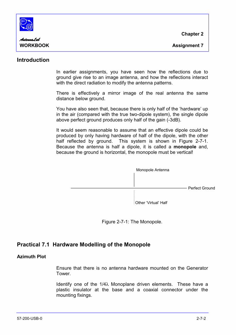
It would seem reasonable to assume that an effective dipole could be produced by only having hardware of half of the dipole, with the other half reflected by ground. This system is shown in Figure 2-7-1. Because the antenna is half a dipole, it is called a monopole and, because the ground is horizontal, the monopole must be vertical!

Figure 2-7-1: The Monopole.

Practical 7.1 Hardware Modelling of the Monopole

Azimuth Plot

Ensure that there is no antenna hardware mounted on the Generator Tower.

Identify one of the 1/4λ Monoplane driven elements. These have a plastic insulator at the base and a coaxial connector under the mounting fixings.

Perfect Ground

Monopole Antenna

Other ‘Virtual’ Half


57-200-USB-0 2-7-3

Identify the Ground Plane and mount the monopole centrally, with nuts and screws provided.

Attach the coaxial cable from the Generator Tower to the connector at the base of the monopole and then attach the monopole/ground plane assembly to the Generator Tower, as shown in Figure 2-7-2.

Figure 2-7-2: Monopole Assembly on Tower


Launch a signal strength vs. angle 2D graph window and immediately switch on the Motor Enable switch.


Also, the Receiver antenna must be changed to the vertical plane. Loosen the knurled screw that is situated in the centre of the four antennas and turn the antennas through 90°.

Acquire a new plot at 1500 MHz.


Question 7.1.1

Is your plot of the shape that you would expect?


57-200-USB-0 2-7-4

Elevation Plot

Remove the Ground Plane/Antenna assembly from the top of the Generator Tower and re-mount it on the side of the Tower, as shown in Figure 2-7-3.

Figure 2-7-3: Antenna Mounting for Elevation Plot

The Receiver antenna must be changed back to the horizontal plane. Loosen the knurled screw that is situated in the centre of the four antennas and turn the antennas through 90°, so that they are horizontal once more.


Question 7.1.2

Is your plot of the shape that you would expect?

Question 7.1.3

Why do you think that you get some radiation below the 90°°°°-270°°°° line?

Practical 7.2 Software Simulation of the Monopole

Run NEC-Win and click New File on the toolbar.

Enter the co-ordinates of the two ends of the monopole into the table as (0, 0, 0) and (0, 0, 0.05) metres.

Enter the diameter of the wire as 0.004 metres (4cm).


57-200-USB-0 2-7-5

Enter 7 segments.

Click on the Src/Ld box and place a source at segment 1.

Use perfect conductors.

Ensure that perfect ground is set and that the frequency is set to 1500 MHz.

Click on Save As and save as mono1.


Question 7.2.1

How do the plots compare with those obtained by hardware modelling?

Question 7.2.2

Do you get radiation below ground with the theoretical simulation?

Question 7.2.3

What is the gain of this antenna along the horizontal?

Question 7.2.4

How does this compare with the gain of a dipole (in free space)?

The dipole in free space is radiating at all vertical angles, whereas the monopole above a perfect ground theoretically only radiates in directions above ground.

Question 7.2.5

Could this account for the extra gain associated with the monopole?

Real Ground

Go back to the main NEC-Win table and change the ground to Real Ground and select the Urban and Industrial Area preset.

Replot the graphs.


57-200-USB-0 2-7-6

Question 7.2.6

Has the gain changed, if so, how?

Question 7.2.7

Ignoring the radiation from behind the Ground Plane, does the shape of this plot compare with the real plot obtained from hardware modelling?

Thus the monopole has an omni-directional azimuth pattern with a gain over a free space dipole of 3dB when operated over perfect ground

In any practical set-up the ground would not be perfect, so there will be a lowering of gain and an increase in vertical angle of the lobes.


57-200-USB-0 2-8-1

ASSIGNMENT 8 PHASED MONOPOLES

Objectives


• appreciate that changes in spacing between two driven monopoles affects the polar pattern,

• appreciate that changes in phase between two driven monopoles affects the polar pattern,

Knowledge Level








• read the ‘Phased Array’ section of Chapter 8 of the ARRL Antenna Book.


57-200-USB-0 2-8-2

Introduction

In Assignment 4, the effects of combining two dipoles have been investigated and it has been seen how the radiation patterns were changed relative to a single dipole.

In this assignment, two monopoles will be combined and the changes due to different spacing and feeding the monopoles in different phases will be investigated.

Practical 8.1 Hardware Modelling of Two Monopoles

Azimuth Plot


Identify the two 1/4λ Monopole driven elements. These have a plastic insulator at the base and a coaxial connector under the mounting fixings.

Identify the Ground Plane and mount one monopole centrally, with nuts and screws provided. Mount the other monopole at a spacing of 5cm from the first.

Identify the 2-way Combiner and also the two 183mm Coaxial Cables. Connect one of these cables to each of the monopoles and their other ends to the two connectors close together on the Combiner.

Attach the coaxial cable from the Generator Tower to the remaining connector on the Combiner.

Attach the monopole/ground plane assembly to the Generator Tower, as shown in Figure 2-8-1.

Figure 2-8-1: Two Monopole Assembly on Tower


57-200-USB-0 2-8-3

Ensure that the Motor Enable switch is off and switch on the Trainer.

Launch a signal strength vs. angle 2D polar graph window and immediately switch on the Motor Enable switch.


The Receiver antenna array must have its elements vertical.



Changing Phase

The above plot has been taken with the two monopoles driven in phase with each other.

Let us now see the effect of changing the phase of one of the monopoles with respect to the other.

Identify the 155mm length of coaxial cable and replace one of the 183mm lengths with it.

This difference in lengths of feeder relates to a phase difference of 90° at 1500 MHz.


The new polar plot will be taken and displayed.

Question 8.1.1

Are the two plots different?

Question 8.1.2

Which phase of feeding leads to the greater directivity?


57-200-USB-0 2-8-4

Question 8.1.3

What is the difference between the forward gain and the gain in the backwards direction for the monopoles fed with 90°°°° phase difference?

This difference for a directive antenna is often known as the front-to-back ratio.

Changing Spacing

Move one of the monopoles to another mounting position to change the spacing between them and replace the 155mm length of coaxial cable with the 183mm length so that the monopoles are again driven in phase.


The third polar plot will be taken and displayed.

Question 8.1.4

Does a change of spacing have an effect?

Practical 8.2 Software Simulation of Two Monopoles

Azimuth Plot

Run NEC-Win and click Open File on the toolbar. Open file mono1.

Now put in another monopole, spaced by 5mm from the first. To do this, enter the co-ordinates of the two ends of the second monopole into the table as (0.05, 0, 0) and (0.05, 0, 0.05) metres.

Enter the diameter of the wire as 0.004 metres (4cm).

Enter 7 segments.

Click on the Src/Ld box and place a source at segment 1.

Use perfect conductors.

Ensure that perfect ground is set and that the frequency is set to 1500 MHz.


57-200-USB-0 2-8-5

Click on Save As and save as 2mono.


Question 8.2.1

How does the azimuth plot compare with the one found using the hardware when the monopoles were fed in phase?

Changing the Phase

Go back to the main NEC-Win table and click on the Src/Ld box of Wire 2.

Click on the green icon for the source and change the phase of the source to 90°.

Click on the Run NEC button and then examine the azimuth plot produced.

Question 8.2.2

How does the azimuth plot compare with the one found using the hardware when the monopoles were fed 90°°°° out of phase?

Changing to Current Feed

Go back to the main NEC-Win table and click on the Src/Ld box of Wire 1.

Click on the green icon for the source and change the source to Current Source

Do the same for Wire 2.

Click on the Run NEC button and then examine the azimuth plot produced.

Question 8.2.3

How does the new azimuth plot compare with the one found using the hardware when the monopoles were fed 90°°°° out of phase?


57-200-USB-0 2-8-6

Question 8.2.4

How does the new azimuth plot compare with the ones found in the ARRL Antenna Book?

From this Assignment you should have found that changes in spacing between two driven antennas, of changes in the relative phases by which they are driven, has a significant effect on the radiation pattern for the system.

The ability to get more directivity, or to ‘beam’ the radiation in a specific direction, is an important property of many antenna systems in practice


57-200-USB-0 2-9-1

ASSIGNMENT 9 RESONANCE, IMPEDANCE AND STANDING WAVES

Objectives


• understand the terms ‘resonance’, ‘impedance’ and VSWR as applied to antennas,

• have determined the resonant frequency and impedance and measured the VSWR of a dipole antenna.

Knowledge Level

You should have an understanding of the terms ‘resonance’ and ‘impedance’.







• read the ‘Phased Array’ section of Chapter 8 of the ARRL Antenna Book.


57-200-USB-0 2-9-2

Introduction

In this assignment the relationship between the length of an antenna and its frequency of operation is investigated, together with the impedance that an antenna exhibits and how this effects its feed requirements.

Practical 9.1 Effects of Antenna Length using Hardware Modelling

Azimuth Plot


Identify one of the Yagi Boom assemblies. Remove all the antenna elements except the dipole and then mount this assembly on top of the Generator Tower.

Position the dipole centrally above the Tower.

Attach the coaxial cable from the Generator Tower to the connector on the boom.


Launch a signal strength vs. angle 2D polar plot and immediately switch on the Motor Enable switch.



57-200-USB-0 2-9-3

The Receiver antenna array must have its elements horizontal.

Set the length of the dipole to its minimum by ensuring that the adjustable ends are both pushed completely in.



Readjust the length of the dipole to 10cm. Ensure that both sides of the dipole are of equal length.


A polar plot will be taken and superimposed on the first.

Now, readjust the length of the dipole to 12cm. The dipole will be almost at its full extent. Ensure that both sides of the dipole are of equal length.


A polar plot will be taken and superimposed on the previous two.

Question 9.1.1

Are there differences in the polar patterns?

Examine the figures down the left-hand side of the screen for the three plots.

Question 9.1.2

Is the gain of the antenna dependent on its length?

Practical 9.2 Antenna Impedance

When an antenna is connected to the end of a transmission line (e.g. coaxial cable), power can be transmitted along the cable, into the antenna and then radiated into space. As far as the source and cable are concerned, the antenna acts like a load on the end of the cable into which power is passed and then is dissipated. Any load has an impedance, which may be resistive, or comprise both resistive and reactive parts.


57-200-USB-0 2-9-4

We will now use NEC-Win to investigate the impedance of a dipole.


Check that the Y co-ordinates for the dipole are –0.05 and +0.05 and ensure that No Ground is set.

Set the Start Frequency to 1300MHz, the Stop Frequency to 1400 MHz and the Step Size to 10 MHz.

Click on the Run NEC button.

Click on the Z button. Select Real and Imaginary parts to be shown and then select OK.

You will notice that the curves of both real (resistive) and imaginary (reactive) parts are plotted.

Examine the imaginary part of the impedance.

Question 9.2.1

Is there a frequency that gives a minimum reactive part?

Theoretically, there will be a frequency at which the reactive (imaginary) part goes to zero. At this frequency, the antenna presents a purely resistive load to the cable.

This frequency is termed the resonant frequency of the antenna (it is like the resonant frequency of a tuned circuit where its impedance is purely resistive).

Many antennas are operated at their resonant frequencies, but an antenna does not have to be resonant to operate properly.

Radiation Resistance

Firstly, read the section on Radiation Resistance in Chapter 2 of the ARRL Antenna Book.


57-200-USB-0 2-9-5

The input impedance is defined as the sum of the radiation resistance and the losses of the antenna. These losses are made up of conductor resistance and dielectric losses in insulators and, possibly, due to the proximity of the antenna with the ground. In a well-designed antenna these losses are very small: perhaps only one, or two percent, thus the radiation resistance is almost the same as the input impedance.

Question 9.2.2

What is the value of the resistive part of the input impedance of your dipole at resonance?

Theoretically, this value should be 73Ω.

Practical 9.3 Standing Waves

The ‘maximum power transfer theorem’ states that the condition required to get maximum efficiency of power transfer from a source to a load is when the source and load are ‘conjugately matched’. This means that the real (resistive) parts of the source and load impedances are equal and the imaginary (reactive) parts are equal in magnitude, but of opposite sign – so that they cancel each other out. Matching of source and load is important in antenna systems, as a high efficiency is usually needed.

In an antenna system, to couple the source (generator) to the load (antenna) requires some sort of cable – like the coaxial cable used in the Antenna Systems Trainer. This cable is often called the ‘transmission line’.

The construction of any practical transmission line will affect its properties. The conductor material will have some resistance (though it is chosen to be as small as possible). There will be capacitance between the two conductors of the line and there will also be inductance associated with the conductors of the line. All of these give rise to the fact that there will be an impedance associated with a transmission line, the value of which will be dependant on the physical construction of the line.

This impedance is called the ‘characteristic impedance’ of the line.


57-200-USB-0 2-9-6

In a properly matched antenna system the output impedance of the generator, the characteristic impedance of the transmission line and the antenna input impedance will all be the same.

If this is so, all the power generated by the source will all flow down the transmission line into the antenna and will then be radiated into space.

What happens if we have a mismatch?

Suppose that the source and the transmission line are matched, but the antenna does not have the same input impedance as the characteristic impedance of the line. The conditions required for maximum power transfer at the antenna end of the transmission line are now not present.

Some of the power transmitted up the transmission line from the source will not be radiated by the antenna. It has to go somewhere, so it is reflected back down the line towards the source.

Both the power from the source to the load (forward power) and the reflected power from the antenna towards the source are in the form of electromagnetic waves and will add where their waves are in phase and will cancel out where they are in antiphase. This gives rise to a pattern of maxima and minima on the transmission line. This pattern is stationary on the line and is called a ‘standing wave’ pattern.

The ratio of the magnitudes of the maximum voltage in this pattern to the minimum voltage is called the ‘voltage standing wave ratio’ and is usually abbreviated to ‘VSWR’.

Read the section on ‘Basic Theory of Transmission Lines’ in chapter 24 of the ARRL Antenna Book to be able to understand this better.

Return to the main NEC-Win table and press the SWR button.

Question 9.3.1

What is the VSWR at resonance for the dipole with a 50ΩΩΩΩ transmission line?

Again, return to the main NEC-Win table. Click on where it says ‘Zo = 50 Ohm’ in the Radiation Pattern box and select 75 Ohm.


57-200-USB-0 2-9-7

Click on SWR and examine the plot produced.

Question 9.3.2


Question 9.3.3

Is it different from the 50ΩΩΩΩ case?

Again, return to the main NEC-Win table and change the Zo to ‘Custom’. Enter 73 as the value.

Click on SWR and examine the plot produced.

Question 9.3.4


You will find that the VSWR approaches 1:1 as you get closer and closer to a true match.

Question 9.3.5

What does that tell you about the maxima and minima on the transmission line if the system is correctly matched?

Practical 9.4 Measurement of VSWR


Navigate to the Return Loss vs. Frequency application page and read the instructions given.

Identify one of the Yagi Boom Assemblies and mount it on top of the Generator Tower.


Launch a return loss vs. frequency graph window and immediately switch on the Motor Enable switch.


57-200-USB-0 2-9-8


Set the dipole length to 10cm.

Identify the Directional Coupler. It is a printed circuit board with four coaxial sockets on it.

Connect it up as detailed in the instructions for the reference power level (forward power reference).

From the menu, click on ‘File’ then ‘New Plot’. Accept the default frequency of 1500 MHz.

The reverse power measurements may now be taken. Connect up the directional coupler as detailed in the instructions. Click ‘OK’ when ready to proceed.

Question 9.4.1

Does the plot have a minimum VSWR (see right-hand-side scale)?

Question 9.4.2

What is the minimum value?

Question 9.4.3

Does the frequency of this minimum agree with that from the software simulation?

Note that there are other frequencies that give dips in the VSWR plot, but that none is so low as at resonance.


57-200-USB-0 2-10-1

ASSIGNMENT 10 RETURN LOSS AND VSWR MEASUREMENTS

Objectives


• understand the terms ‘VSWR’ and ‘return loss’,

• have measured the VSWR for short circuit, open circuit and matched conditions

• have investigated the VSWR and return loss of a dipole antenna.

Knowledge Level









57-200-USB-0 2-10-2

Introduction

In Assignment 9, you have seen how to take VSWR measurements with AntennaLab. In this assignment you will be investigating the measurement of VSWR in more detail.

Practical 1 Open and Short Circuit and 50ΩΩΩΩ Loads





Launch a return loss vs. frequency graph window and immediately switch on the Motor Enable switch.



Identify the Directional Coupler. Connect it up as detailed in the instructions for the reference power level (forward power reference), but do not attach the cable to the antenna.

Ensure that the directional coupler is kept as far as possible from the other equipment.

From the menu, click on ‘File’ then ‘New Plot’. Accept the default frequency of 1500 MHz.



57-200-USB-0 2-10-3

Question 10.1.1

How does the VSWR vary with frequency (see right-hand-side scale)?

Identify and connect the short circuit to the antenna socket of the Directional Coupler and repeat the VSWR measurements.

Question 10.1.2

How does the VSWR vary with frequency, now?

Question 10.1.3

With an open or a short circuit load, is the VSWR high, or low?

Identify and connect the 50Ω load to the antenna socket of the Directional Coupler and repeat the VSWR measurements.

Question 10.1.4

How does the VSWR vary with frequency, now?

Question 10.1.5

With a 50ΩΩΩΩ load, is the VSWR high, or low?

In theory, the VSWR for either a short, or an open circuit load should be infinite (∞:1).

The scale on the VSWR plot on the Antenna Systems Trainer only goes up to just above 10:1, however, the practical plots are at this level, showing high VSWR. The cyclic dips that you see in the VSWR plots are due to imperfections in the directional coupler, as it is almost impossible to produce a perfect coupler to work over this wide frequency range.

Practical 10.2 VSWR of a Dipole

Connect up the dipole to the antenna socket of the directional coupler and repeat the VSWR measurements.

Examine the main dip in the response at just above 1300 MHz.


57-200-USB-0 2-10-4

Question 10.2.1

Does the VSWR change abruptly or gradually with frequency about this minimum?

Question 10.2.2

Over what range of frequencies is the VSWR below 2:1 about this minimum?

Because the input impedance of the dipole is not constant with frequency, the VSWR on the transmission line will not be constant with frequency either.

The dipole has a much lower bandwidth over which the VSWR is low than, for example, the 50Ω resistive load.

As we will see in later assignments, other antennas have even narrower bandwidths.

Return Loss

Another way of expressing how well an antenna is matched is by quoting its ‘return loss’.

The return loss is related to the VSWR by the following equation:

VSWR = (1 + k)/(1 – k)

Where k = 10exp( –RL/20)

RL is the return loss, expressed in dB.

The equivalent return loss, in dB, is shown down the left-hand side of the plots.

Question 10.2.3

What is the approximate equivalent return loss, in dB, to a VSWR of 2:1?


57-200-USB-0 2-11-1

ASSIGNMENT 11 PARASITIC ELEMENTS

Objectives


• have investigated the properties of a system comprising a dipole and a parasitic element,

• understand the terms ‘driven element’, ‘reflector’ and ‘director’,

• know the form of a ‘yagi’ antenna.

Knowledge Level

You should have performed Assignments 6 & 8.








57-200-USB-0 2-11-2

Introduction

In Assignment 6, the effects of the ‘image’ of an antenna due to ground reflections were investigated. It was shown that there is an increase in gain (in some directions) when an antenna is brought close to ground, due to the effective ‘extra’ image antenna.

What happens when two antennas were positioned close to each other and both driven was investigated In Assignment 8.

In this assignment, the effect of positioning a second, un-driven, real antenna close to the driven one is investigated.

Practical 11.1 Two Dipole Elements


Ensure that all of the elements are removed, except for the dipole, and that this is mounted above the tower support.


Launch a signal strength vs. angle 2D polar graph window and immediately switch on the Motor Enable switch.



Acquire a new plot at 1500MHz.

Observe the polar plot obtained.

Identify on of the other un-driven dipole antenna elements that are supplied with the Antenna Systems Trainer.

Move the driven dipole forward on the boom by about 2.5cm and mount a second un-driven dipole element behind the first, at a spacing of about 5cm.


57-200-USB-0 2-11-3

Set the un-driven dipole length to 10cm.


Question 11.1.1

Has the polar pattern changed by adding the second element?

Question 11.1.2

Has the gain changed by adding the second element?

Question 11.1.3

Has the directivity changed by adding the second element?

Change the spacing between the two elements of the antenna to 2.5cm.


Question 11.1.4

What changes has the alteration in spacing made to the gain and directivity?

Practical 11.2 Changing the Length of the Parasitic Element

Set the spacing between the two elements to 2.5cm and ensure the lengths of both the elements are 10cm.

Launch a new signal strength vs. angle 2D polar graph window.


Extend the length of the un-driven element to 11cm.


Reduce the length of the un-driven element to 8cm.


Question 11.2.1

What changes has the alteration in length made to the gain and directivity?


57-200-USB-0 2-11-4



Check that the Y co-ordinates for the dipole are –0.05 and +0.05 and ensure that No Ground is set.

Click on the cell of the table that has the figure 1 in it under Wire on the left-hand column of the table. This will highlight the Wire 1 row.

Click on the Copy button on the toolbar, to copy this row to the clipboard.

Now highlight row ‘Wire 2’ by clicking on the 2 in the Wire column.

Click on the Paste button in the toolbar to paste into the Wire 2 row.

The second dipole must now be placed 2.5cm behind the first. Change X1 and X2 for Wire 2 to be –0.025 to do this. Verify that you have done this correctly by looking at NEC-Vu.

The second dipole is not going to be driven, so you need to remove the source from Wire 2. Click on the Src/Ld cell for Wire 2 and then drag the green source icon into the bin at the bottom right-hand corner. Then click OK.

Save this two element antenna as 2el1.

Look at the plots for this antenna.

Now, change the length of the second dipole element (the Y co-ordinates of Wire 2) to give a total length of 11cm.

Save this antenna as 2el2.

Look at the plots for this antenna.

Now, change the length of the second dipole to give a total length of 8cm.

Save this antenna as 2el3.

Look at the plots for this antenna and add the 2el1 and 2el2 files. Give them different colours so that you can identify which is which.


57-200-USB-0 2-11-5

Question 11.3.1

How do these theoretical, simulated plots compare with the ‘real’ plots obtained from Practical 11.2?

Figure 2-11-1: Typical Simulation Plots

With the length of the second dipole (the un-driven, or ‘parasitic’ element) shorter than the driven dipole (the driven element) the direction of maximum radiation is from the driven element towards the parasitic element. In this case, the parasitic element is called the ‘director’.

With the length of the second dipole longer than the driven dipole the direction of maximum radiation is from the parasitic element towards the driven element. In this case, the parasitic element is called the ‘reflector.

An antenna of this type, with a driven element and one, or more , parasitic elements is generally known as a ‘yagi’, after on of its inventors (Mssrs Yagi and Uda). Assignment 12 investigates yagis in more detail.


57-200-USB-0 2-11-6

Notes

Chapter 2 AntennaLab AntennaLab AntennaLab AntennaLab WORKBOOK Assignment 12

57-200-USB-0 2-12-1

ASSIGNMENT 12 MULTI-ELEMENT PARASITIC ARRAYS

Objectives


• have examined multi-element yagis,

• have seen how gain and directivity increase as element numbers increase,

• appreciate the practical limitations to the number of elements.

Knowledge Level









57-200-USB-0 2-12-2

Introduction

Assignment 11 showed that the addition of a second parasitic dipole element close to the driven dipole gives rise to a change in directivity and an increase in gain in a preferred direction. It also showed that the length of the parasitic element had an effect on the direction of maximum gain. If the parasitic element is the same length, or longer than the driven element the gain is in a direction from parasitic element to driven element. The parasitic element acts as a reflector. If the parasitic element is shorter than the driven element the gain is in a direction from driven element to parasitic element. The parasitic element acts as a director.

This assignment investigates the effects of increasing the number of reflectors and directors on the gain and directivity of an array.

Practical 12.1 Adding a Second Reflector – Hardware Modelling

Identify one of the Yagi Boom Assemblies and mount it on top of the Generator Tower. See Figure 2-12-1.

Figure 2-12-1: Multi-element Yagi Assembly

Ensure that all of the elements are removed, except for the dipole.



57-200-USB-0 2-12-3

Launch a signal strength vs. angle 2D polar graph and immediately switch on the motor enable.


Mount the driven dipole on the boom forward from the axis of rotation by about 2.5cm and mount a second un-driven dipole element behind the first, at a spacing of about 5cm.

Set the dipole length to 10cm and the un-driven dipole length to 11cm.


Observe the polar plot.

Mount a second parasitic element about 5cm from the first parasitic reflector and adjust its length to 11cm.



Question 12.1.1

Is there any significant difference between the two plots?

Change the spacing between the two reflectors and acquire a third new plot at 1500 MHz.

Question 12.1.2

Is there any significant difference between the plots, now?

You will find that the addition of a second reflector has little effect on the gain and directivity of the antenna, irrespective of the spacing between the two reflectors.

Practical 12.2 Adding Directors

Remove the second reflector element from the boom.


57-200-USB-0 2-12-4

Launch a new signal strength vs. angle 2D polar graph window.



Mount a parasitic element about 5cm in front of the driven element and adjust its length to 8.5cm.



Question 12.2.1

Is there any significant difference between the two plots?

Move the director to about 2.5cm in front of the driven element.



Question 12.2.2

How does the new plot compare with the previous two?

Launch another new signal strength vs. angle 2D polar graph window.


Add a second director 5cm in front of the first.


Add a third director 5cm in front of the second.


Add a fourth director 5cm in front of the third.

Acquire a fourth new plot at 1500 MHz.

Question 12.2.3

How do the gains and directivities compare?

Launch another new signal strength vs. angle 2D polar graph window.


57-200-USB-0 2-12-5


Move the reflector to 2.5cm behind the driven element. Acquire a second new plot at 1500 MHz.

Question 12.2.4

Does the driven element – reflector spacing have much effect on the gain or directivity of the antenna?


Identify the Directional Coupler. Connect it up as detailed in the instructions for the reference power level (forward power reference).

Ensure that the directional coupler is kept as far as possible from the other equipment.

Launch a return loss vs. frequency graph window.

From the menu, click on ‘File’ then ‘New Plot’. Accept the default frequency of 1500MHz.


Move the reflector to 5cm behind the driven element.

Acquire a second new plot.

Question 12.2.5

Between which frequencies is the VSWR 2:1, or less, for the 2.5cm reflector spacing?

Question 12.2.6

Between which frequencies is the VSWR 2:1, or less, for the 5cm reflector spacing?

Question 12.2.7

Does the narrow, or the wide spacing give the greater VSWR bandwidth?


57-200-USB-0 2-12-6


Run NEC-Win and click Open File on the toolbar. Open file 2el2.

Check that the Y co-ordinates for the dipole are -0.05 and +0.05 and ensure that No Ground is set.

Check that the Y co-ordinates for the reflector are -0.055 and +0.055 and change the X co-ordinates to -0.05. This gives a 5cm spacing between driven element and reflector.

Copy Wire 2 into Wire 3 and then, for Wire 3, enter Y co-ordinates of +0.0425 and -0.0425 and X co-ordinates of +0.025, corresponding to an element length of 8.5cm and a spacing of 2.5cm between driven element and director.

Verify that you have done this correctly by looking at NEC-Vu.

Ensure that there are no sources associated with Wires 2 and 3.

Save this three element antenna as 3el1.

Run NEC for this antenna.

Copy Wire 3 into Wire 4 and then, for Wire 4, enter Y co-ordinates of +0.075, corresponding to an element length of 8.5cm and a spacing of 5cm between the two directors.


Save this four element antenna as 4el1.


Copy Wire 4 into Wire 5 and then, for Wire 5, enter Y co-ordinates of +0.125, corresponding to an element length of 8.5cm and a spacing of 5cm between the directors.


Save this five element antenna as 5el1.



57-200-USB-0 2-12-7

Copy Wire 5 into Wire 6 and then, for Wire 6, enter Y co-ordinates of +0.175, corresponding to an element length of 8.5cm and a spacing of 5cm between the directors.


Save this six element antenna as 6el1.


Click on the Pattern Plot button and then add the 3el1.nou, 4el1.nou and 5el1.nou files.

Select the azimuth plots and superimpose them, choosing different colours for each.

Question 12.3.1

Do the software plots agree, generally, in shape with those modelled with the hardware?

Question 12.3.2

How do the gains and directivities compare?

Now, select the elevation plots and superimpose them, choosing different colours for each.

Question 12.3.4

Are the plots as directive in the elevation plane?

Generally, as the number of elements goes up so does the forward gain and the directivity. However, there is a diminishing return. In practice, the increase in gain from a dipole to a 2 element yagi is just less than 3dB. Adding a director to make a 3 element yagi generally increases the gain by about 2dB. Another director to make a 4 element yagi will perhaps give another 1dB, and so on.

Theoretically, doubling the number of elements should double the gain (+3dB). In practice this is never achieved – perhaps 2dB or 2.5dB only.


57-200-USB-0 2-12-8

Notes


57-200-USB-0 2-13-1

ASSIGNMENT 13 STACKED & BAYED ARRAYS

Objectives


• understand the terms ‘baying’ and ‘stacking’ as applied to antennas,

• have investigated stacked and bayed yagi antennas,

• have compared their performance with a single yagi.

Knowledge Level









57-200-USB-0 2-13-2

Introduction

Yagi antennas may be used side-by-side, or one on top of another to give greater gain or directivity. This is referred to as baying, or stacking the antennas, respectively.

In this assignment these combinations will be investigated. See Figure 2-13-1 and Figure 2-13-2 for views of the assemblies required for this assignment.

Figure 2-13-1: Bayed yagi assembly 1

Figure 2-13-2: Stacked yagi assembly

Practical 13.1 Baying two Yagis

Ensure that a Yagi Boom Assembly is mounted on the Generator Tower.


57-200-USB-0 2-13-3

Build up a 6 element yagi, identical to that used in Assignment 12. The dimensions of this are:

Length Spacing

Reflector 11cm 5cm behind driven element

Driven Element 10cm zero (reference)

Director1 8.5cm 2.5cm in front of DE

Director2 8.5cm 5cm in front of D1



Plot the polar response at 1500 MHz.

Without disturbing the elements too much, remove the antenna from the Generator Tower.

Identify the Yagi Bay base assembly (the broad grey plastic strip with tapped holes) and mount this centrally on the Generator Tower.

Mount the 6 element yagi onto the Yagi Bay base assembly at three holes from the centre.

Assemble an identical 6 element yagi on the other Yagi Boom Assembly and mount this on the Yagi Bay base assembly at three hole the other side of the centre, ensuring that the two yagis are pointing in the same direction (towards the Receiver Tower).

Identify the 2-Way Combiner and the two 183mm coaxial cables.

Connect the two 183mm cables to the adjacent connectors on the Combiner and their other ends to the two 6 element yagis.

Connect the cable from the Generator Tower to the remaining connector on the Combiner.

Acquire a new plot for the two bayed antennas onto the same graph as that for the single 6 element yagi.

Reverse the driven element on one of the yagis and acquire a third plot.


57-200-USB-0 2-13-4

Question 13.1.1

Does reversing the driven element make much difference to the polar pattern for the two bayed yagis?

Question 13.1.2

How does the directivity of the two bayed yagis compare with the single yagi plot (with the driven element the correct way round)?

Question 13.1.3

How does the forward gain of the two bayed yagis compare with the single yagi plot (with the driven element the correct way round)?

Now, move the two yagis to the outer sets of holes on the Yagi Bay base assembly. Ensure that you keep the driven elements the same way round as you had before to give the correct phasing.

Superimpose a plot for this assembly.

Question 13.1.4

How do the directivity and forward gain of the wider spaced yagis compare with the close spaced yagis?

Notice the side-lobes of the forward pattern.

Practical 13.2 Stacking Two Yagis

Identify the Yagi Stack base assembly (the narrow grey plastic strip with tapped holes) and mount this on the side of the Generator Tower.

Mount the 6 element yagi onto the Yagi Stack base assembly at one set of holes above the centre.

Plot the polar response at 1500 MHz.

Mount the other 6 element yagi on the Yagi Stack base assembly at the uppermost set of holes, ensuring that the two yagis are pointing in the same direction (towards the Receiver Tower).

Identify the 2-Way Combiner and the two 183mm coaxial cables.


57-200-USB-0 2-13-5

Connect the two 183mm cables to the adjacent connectors on the Combiner and their other ends to the two 6 element yagis.

Connect the cable from the Generator Tower to the remaining connector on the Combiner.

Superimpose the polar plot for the two stacked antennas onto that for the single 6 element yagi.

Reverse the driven element on one of the yagis and superimpose a third plot.

Change the position of the lower yagi to the bottom set of holes on the Yagi Stack base assembly. Ensure that the driven elements are correctly phased and superimpose a fourth polar plot.

Question 13.2.1

How does the directivity of the different configurations compare?

Question 13.2.2

How does the forward gain of the stacked yagis compare with the single yagi?

Question 13.2.3

How does the forward gain of the stacked yagis change when the driven element phasing is incorrect?

Practical 13.3 Software Simulation of Stacking and Baying

Run the NEC-Win software and open file 6el1.

Copy the six wires of 6el1 into wires 7-12. Use the Translate button to translate the X co-ordinates of the first yagi +8cm and those for the second yagi –8cm.

Look at NEC-Vu to verify that you have separated the two yagis correctly.

Save the file as 2x6el1.

Plot the polar response.


57-200-USB-0 2-13-6

Change the spacing of the yagis to ±12cm and plot the response.

Compare the responses and with those found using hardware modelling.

Repeat the same procedure for stacked yagis.

Arrays of yagis: stacked, bayed, or both, are used in practice to achieve higher gains than can be achieved with single antennas. However, there is a ‘law of diminishing returns’ in that to get 3dB (theoretical) gain improvement requires a doubling of the antenna: e.g. stacking two 6 element yagis gives almost 3dB increase, another two would be required to give a further 3dB and another four to give another 3dB.

In practice, imperfections in the feed systems for such complicated arrays of antennas mean that much less than 3dB is achieved, making it generally uneconomical to use more than two antennas.


57-200-USB-0 2-14-1

ASSIGNMENT 14 THE HORN ANTENNA

Objectives


• have investigated the gain and directivity of a horn antenna,

• have investigated the frequency response and VSWR of a horn antenna.

Knowledge Level








57-200-USB-0 2-14-2

Introduction

The horn antenna is a type that is often used at UHF and Microwave frequencies. It may be used as a reflecting and directing structure associated with a simple driven element, such as a dipole or a monopole, or it may be used to terminate a length of waveguide to launch radiation into space.

The horn used in AntennaLab is of the first type – the driven element being a monopole.

This assignment investigates its performance. See Figure 2-14-1 for a view of the assembly for this assignment.

Figure 2-14-1: Horn assembly

Practical 14.1 Gain and Directivity of a Horn

Mount the Yagi Boom assembly on top of the Generator Tower and position the dipole at the centre, directly above the tower.

Set the length of the dipole to 10cm.

Plot the polar response of the dipole.

Remove the Yagi Boom assembly from the tower.

Identify the Waveguide Horn. Mount a driven monopole element inside the horn by the holes at the rear of the horn.


57-200-USB-0 2-14-3

Mount the horn on the Generator Tower with the monopole element vertical and connect up the monopole to the coax cable from the Generator.

Set the length of the monopole to its minimum.

Set the polarisation of the Receiver antenna to be vertical.

Plot the polar response of the horn.

Question 14.1.1

What is the gain of the horn with respect to the dipole?

Question 14.1.2

Does the horn have directivity?

Question 14.1.3

Why do you think there is a back lobe in the polar response of the horn?

Acquire a signal strength vs. frequency plot for the horn.

Question 14.1.4

Is the response of the antenna greatly dependent on frequency?

Now plot the Return Loss (VSWR) of the horn.

Question 14.1.5

Is the VSWR response of the antenna greatly dependent on frequency?

Question 14.1.6

Is the VSWR of the antenna good, or bad?

Question 14.1.7

What does this tell you about the impedance of the antenna?


57-200-USB-0 2-14-4

Although the horn antenna may be used as a reflecting and directing structure, as it is in this Assignment, the most common use of a horn antenna is as a feed antenna at the focus of a dish reflector.

This form of antenna is commonly used in satellite broadcasting for both receiving and transmitting systems.


57-200-USB-0 2-15-1

ASSIGNMENT 15 THE LOG PERIODIC ANTENNA

Objectives


• be familiar with the log periodic form of antenna,

• have investigated the gain, directivity and VSWR of the log periodic antenna over a wide frequency range,

• appreciate the advantages and disadvantages of a log periodic antenna as compared with a yagi.

Knowledge Level








57-200-USB-0 2-15-2

Introduction

The yagi antennas that you have been investigating are inherently narrow-bandwidth antennas. The relatively small range of frequencies over which the VSWR is below 2:1 has demonstrated this.

The log periodic antenna is a design that attempts to cover a much wider bandwidth. With a yagi all of the elements are active on the operating frequency. With a log periodic antenna only a number of the elements will be active on any one frequency, the actual elements that are active changing as the frequency is changed.

For much more information on log periodic antennas, see Chapter 10 in the ARRL Antenna Book.

See Figure 2-15-1 for a view of the assembly required for this assignment.

Figure 2-15-1: Log periodic assembly

Practical 1 Hardware Measurements



Plot the polar response of the dipole at 1500 MHz.


Identify the 5 element Log Periodic Antenna with its feeder cable.


57-200-USB-0 2-15-3

Mount this antenna on the Generator Tower and connect the cables.

Superimpose the polar response for this antenna at 1500 MHz.

Question 15.1.1

Does the log periodic antenna have gain over the dipole at 1500MHz?

Question 15.1.2

Does the log periodic antenna have directivity at 1500MHz?

Using a new graph window, plot the polar response for 1500 MHz again.

Superimpose polar plots for frequencies of 1200 MHz, 1300 MHz and 1400 MHz on the 1500 MHz one.

Question 15.1.3

Does the log periodic antenna have gain over this range of frequencies?

Question 15.1.4

Does the log periodic antenna have directivity at over this range of frequencies?

Restart and plot the polar response for 1500 MHz again.


Question 15.1.5

What happens to the gain of the log periodic antenna over this range of frequencies?

Question 15.1.6

Does the log periodic antenna still have directivity at over this range of frequencies?

Now plot the Return Loss (VSWR) of the horn.


57-200-USB-0 2-15-4

Question 15.1.7

Is the VSWR response of the antenna greatly dependant on frequency?

Question 15.1.8

Is the VSWR of the antenna good, or bad?

Question 15.1.9

What does this tell you about the impedance of the antenna?

The log periodic form of antenna sacrifices gain for bandwidth. At any one frequency only a proportion of the total elements of the log periodic are active – so it performs rather like a yagi with fewer elements. However, as the frequency is changed other elements become active, thus maintaining the performance much more constant over a wide range of frequencies. The impedance, and thus the VSWR, are also more constant over the frequency range.


57-200-USB-0 2-16-1

ASSIGNMENT 16 THE DISH ANTENNA

Objectives


• be familiar with the dish form of antenna,

• have investigated the gain and directivity of the dish antenna,

• appreciate the advantages and disadvantages of a dish antenna as compared with a yagi.

Knowledge Level








57-200-USB-0 2-16-2

Introduction

A dish can be thought of as a passive reflector that focuses the energy from a source into one direction, much like a parabolic mirror focuses light. However, to perform as efficiently as an optical reflector, a dish needs to be in excess of ten wavelengths in diameter for the frequency being used. This is very often not the case in practice, due to physical size constraints.

It was stated in Assignment 14 that the horn antenna is often used to launch, or capture energy from a dish reflector. Although this is quite common, a simple dipole is often used to perform the same task.

The dish set-up with AntennaLab is one that uses a dipole at, or close to, the focus of a 60cm parabolic dish.

See Figure 2-16-1 and Figure 2-16-2 for views of the assembly required for this assignment

Figure 2-16-1 Dish Assembly

Rear View

Figure 2-16-2 Dish Assembly

Front view


57-200-USB-0 2-16-3

The dimensions for a dish are shown in Figure 2-16-3.

Figure 2-16-3: Dish Dimensions

The focal length for a dish such as in Figure 2-16-3 is given by:

f = D2/16d

Practical 1 Hardware Measurements

Because the dish is a physically large structure, the speed of rotation of the system must be lowered for this Assignment, as directed below.



Do not connect up the coaxial cable to the dipole.

Launch a new signal strength vs. angle 2D polar graph.

From the menu select ‘Tools’ then ‘Change Motor Speed’. Select a value of approximately 60% and click ‘OK’.

Now, connect up the cable.

Plot the polar response of the dipole at 1500 MHz.


D

d

f

D = diameter of dish d = depth of dish f = focal length


57-200-USB-0 2-16-4

Identify the Dish Antenna.

Mount the Yagi Boom assembly onto the Dish and position the dipole towards the end with the plane reflector at the end of the boom.

Mount this assembly onto the Generator tower.

Ensure the length of the dipole is 10cm.

Set the distance from the dipole to the dish to be 38cm.

Set the plane reflector 5cm in front of the dipole (further from the dish).

Figure 2-16-4: Dish Assembly

Superimpose a new plot to observe the response of the dish at 1500 MHz.

Question 16.1.1

Does the dish antenna have gain over the dipole at 1500 MHz?

Question 16.1.2

Does the dish antenna have directivity at 1500 MHz?

The gain of a dish is given by:

G = 4ππππaεεεε/λλλλ2


57-200-USB-0 2-16-5

Where G is the gain, a is the area of the dish, εεεε is the dish efficiency and λ is the wavelength. Note that this is dBi, your measured gain will be dBd. For the dish with AntennaLab at 1500 MHz the efficiency is about 0.5.

Question 16.1.3

Does the measured gain of the dish antenna agree with the theoretical gain at 1500 MHz?


Question 16.1.4

Does the dish antenna have gain over this range of frequencies?

Question 16.1.5

Does the dish antenna have directivity over this range of frequencies?

Restart and plot the polar response for 1500 MHz again.


Question 16.1.6

What happens to the gain of the dish antenna over this range of frequencies?

Question 16.1.7

Does the dish antenna still have directivity at over this range of frequencies?

Practical 2 Changing the Positions of the Dipole and the Plane Reflector

Using a new graph window take a polar plot at 1500 MHz.

Reduce the spacing of the plane reflector from the dipole to 4cm and superimpose a second 1500 MHz polar plot.


57-200-USB-0 2-16-6

Increase the spacing to 6cm and superimpose another new plot.

Question 16.2.1

Does the response change significantly?

Reset the spacing to 5cm.

On a new graph take a polar plot at 1500 MHz.

Reduce the distance from the dipole to the dish by 1cm whilst maintaining the spacing of the plane reflector from the dipole of 5cm and superimpose a second 1500 MHz polar plot.

Reduce the distance from the dipole to the dish by another 1cm whilst maintaining the spacing of the plane reflector from the dipole of 5cm and superimpose another 1500 MHz polar plot.

Question 16.2.2

Does the response change significantly?

Try for other distances and reflector spacings.

Question 16.2.3

Is the response of the dish antenna critically dependent on the spacings?

For the frequencies used by AntennaLab the dish is not large enough to be very efficient: much of the radiation reflected by the plane reflector will pass outside the rim of the dish. This is also why the polar plot shows significant rear lobes – they would be much smaller if the dish were larger. However, it can be seen that the gain achievable with a dish is significantly greater than with any other type of antenna tested and that its directivity is high.

The performance of the dish is not greatly dependent on exact positions of dipole and reflector.

Because of its advantages of high gain and directivity, the dish type of antenna is the most used form of antenna for high uhf and microwave applications.

e-learning electricity & electronics control & instrumentation … · 2020. 10. 9. ·...

Documents