Earnings Quality

Yanzhi Wang

Sloan (1996)

This paper aims to study the relation between earnings and earnings components (i.e, cash flows and accruals), and the impact of them on stock return.

Earnings measure in this paper excludes the non-recurring items and is adopted by the EBIT (Compustat Item 178).

Earnings=Cash flows + AccrualsCash flow based accrualsBalance sheet based accruals

Earnings Persistence

Current earnings positively leads future earnings. Thus high current earnings is followed by high stock market return (Ou and Penman, 1989; Bernard and Thomas, 1989; 1990)

They use the mechanical prediction model or an autoregressive model to predict future earnings.

This links to the earnings momentum.

Earnings Fixation

Sloan (1996) turns to look at the earnings components rather than the earnings surprise.

Investors fixate on earnings, failing to distinguish fully between the different properties of the accrual and cash flow components of earnings.

Earnings Persistence and Earnings Components

CFO (cash flow from operations), as a measure of performance, is less subject to distortion than is the net income figure. This is so because the accrual system, which produces the income number, relies on accruals, deferrals, allocations and valuations, all of which involve higher degrees of subjectivity than what enters the determinations of CFO.

The higher the ratio of CFO to net income, the higher the quality of that income.

Hypotheses

H1: The persistence of current earnings performance is decreasing in the magnitude of the accrual component of earnings and increasing in the magnitude of the cash flow component of earnings.

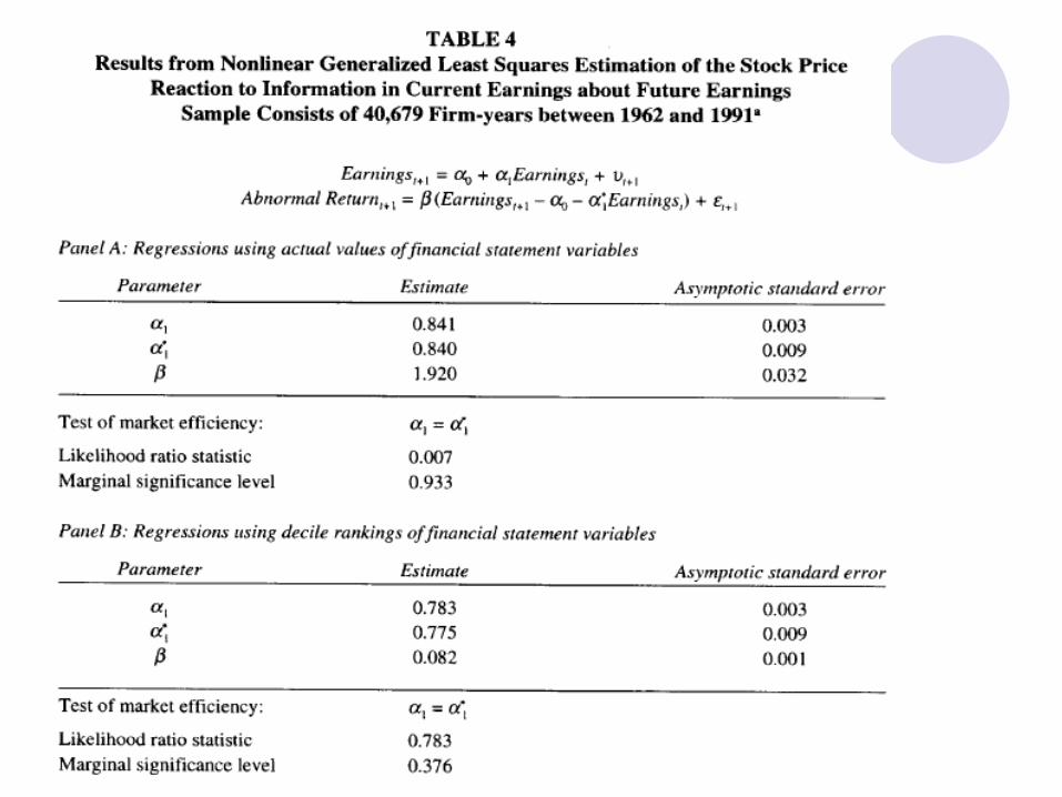
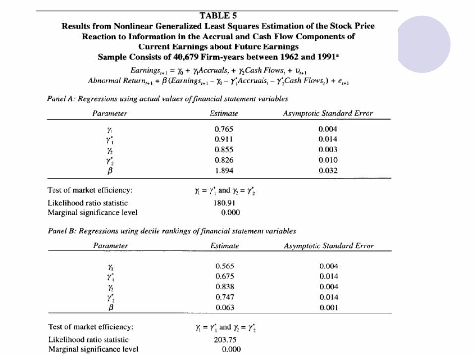
H2(i): The earnings expectations embedded in stock prices fail to reflect fully the higher earnings persistence attributable to the cash flow component of earnings and the lower earnings persistence attributable to the accrual component of earnings.

Hypotheses

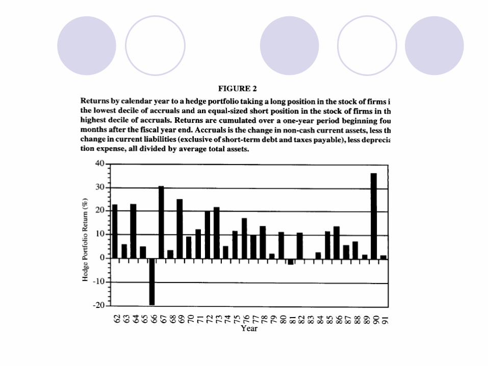
H2(ii):A trading strategy taking a long position in the stock of firms reporting relatively low levels of accruals and a short position in the stock of firms reporting relatively high levels of accruals generates positive abnormal stock return.

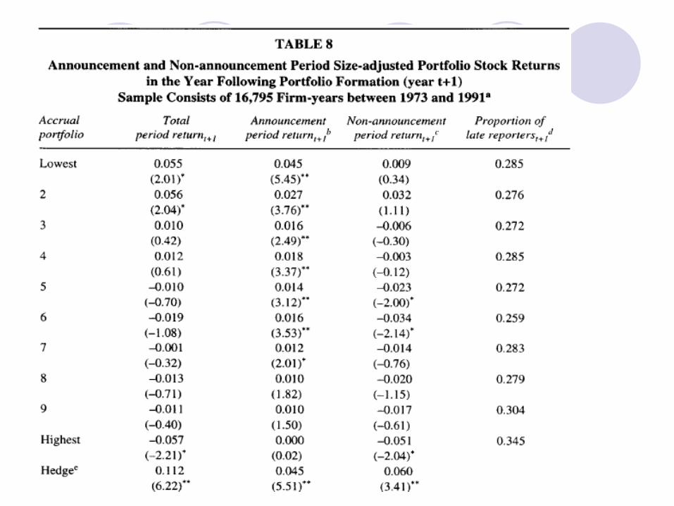
H2(iii):The abnormal stock returns predicted in H2(ii) are clustered around future earnings announcement dates.

Sample

The sample period covers the CRSP/Compustat data from 1962 to 1991.Pre-1962 data suffer from a serious

survivorship bias (Fama and French, 1992)Compustat data availability, especially the

accrual informationRequire at least one year return information

The sample consists of 40,678 firm-year observations.

Accruals

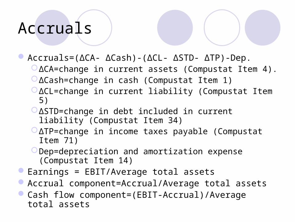
Accruals=(ΔCA- ΔCash)-(ΔCL- ΔSTD- ΔTP)-Dep.ΔCA=change in current assets (Compustat Item 4).ΔCash=change in cash (Compustat Item 1)ΔCL=change in current liability (Compustat Item 5)ΔSTD=change in debt included in current liability

(Compustat Item 34)ΔTP=change in income taxes payable (Compustat Item

71)Dep=depreciation and amortization expense (Compustat

Item 14)Earnings = EBIT/Average total assetsAccrual component=Accrual/Average total assetsCash flow component=(EBIT-Accrual)/Average total

assets

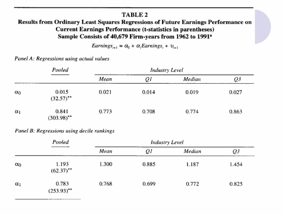
Figure 1

Chan, Chan, Jegadeesh, and Lakonishok (2006)Can accounting information predict stock

returns?Accruals effect (Sloan, 1996)

High (low) accrual firms have low (high) future returns

Why do accruals predict returns?Earnings manipulation hypothesisExtrapolation hypothesisDelayed reaction hypothesis

Definition of Accruals

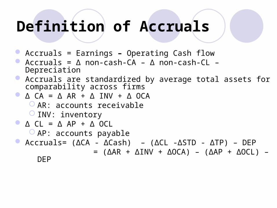
Accruals = Earnings – Operating Cash flow Accruals = Δ non-cash-CA – Δ non-cash-CL – Depreciation Accruals are standardized by average total assets for comparability

across firms Δ CA = Δ AR + Δ INV + Δ OCA

AR: accounts receivable INV: inventory

Δ CL = Δ AP + Δ OCL AP: accounts payable

Accruals= (∆CA - ∆Cash) – (∆CL -∆STD - ∆TP) – DEP = (∆AR + ∆INV + ∆OCA) – (∆AP + ∆OCL) – DEP

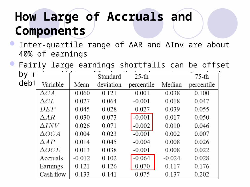
How Large of Accruals and Components

Inter-quartile range of ΔAR and ΔInv are about 40% of earnings Fairly large earnings shortfalls can be offset by not writing off

obsolete inventory or bad debt

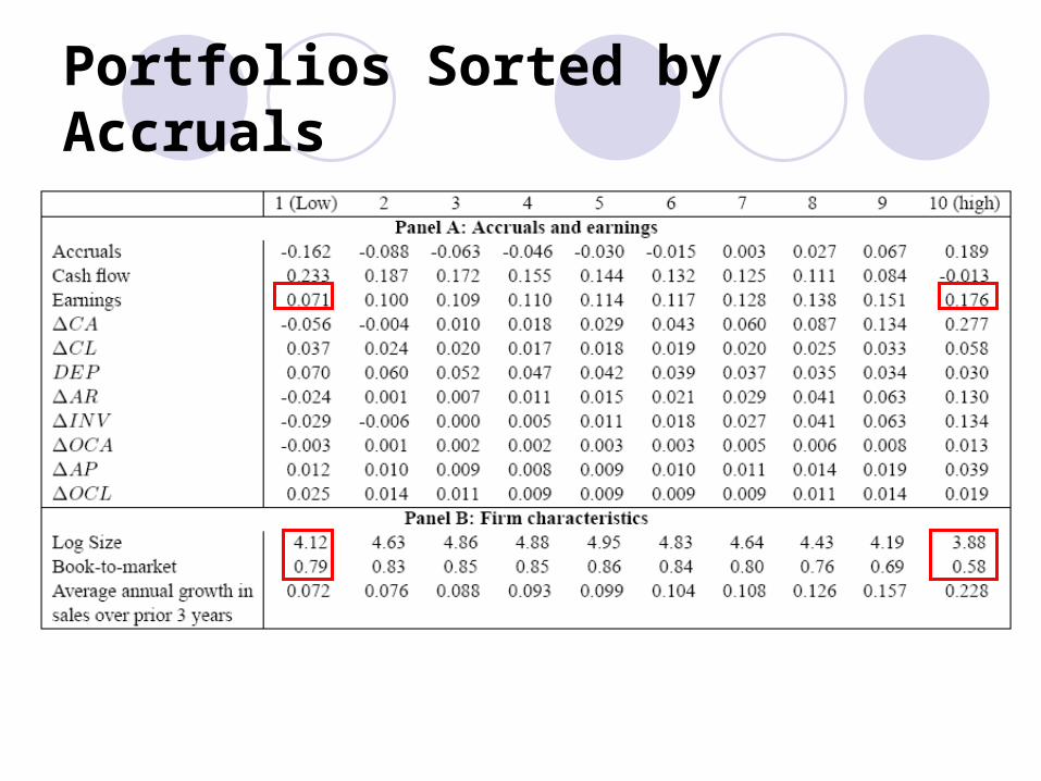
Portfolios Sorted by Accruals

Portfolios Sorted by Accruals

Average annual buy-and-hold returnAR=ΣiΠtrit - ΣjΠtrjt , rj is sample firm daily return,

and rj is daily return for size/BM matching firms

High vs. Low Accrual Portfolios

High accruals firms are high sales growth firmsHigh accruals firms also report large earningsHigh accruals firms experience strong returns

one and two years before rankingLow accruals firms earn higher returns in the

three years following portfolio formationThe hedge portfolio (Low – High) return is

largely due to low returns of high accrual firms

Returns and Components of Accruals

Inventory and Accounts Payable

Changes in inventory predict returns to the same extent as accruals

The sign of the correlation between Accounts Payable and futures returns not consistent with that between accruals and futures returns

What’s High Accruals? Manipulation?

Positive accruals imply cash flow less than earnings

Manipulation hypothesisLarge increases in accounts receivables

indicate bogus salesLarge increases in inventory due to abnormal

less write offsInvestors were fooled by earnings management

Other Hypotheses for High Accruals

Extrapolation hypothesisLarge sales growth will be accompanied by working

capital increases, which cause high accruals Investors extrapolate the current strong sales growth

too far into the futureDelayed reaction hypothesis

High accruals may be due to deteriorating fundamentalsUnexpected slow down in current sales will result in

unsold inventoryCompetitive pressures may force firms to extend more

credit terms Investors overlook the early warning signals in accruals

Discretionary and Non-discretionary Accruals

Non-discretionary accruals: changes in working capital that are required to support sales growth

We model it to be proportional to sales growthDiscretionary accruals

= Total accruals – non-discretionary accrualsDiscretionary accruals

Abnormal accruals after control firm’s business condition

It’s subject to managers’ discretionProxy for the level of earnings manipulation

Measures of Discretionary Accruals

Jones (1991) model (applied in Teoh, Welch and Wong (1998)) to decompose accruals into DA and NDA. Discretionary accruals= residuals of the following regression

CCJL (2006) approach Iit is variable of inventory (or AR, accruals instead)

NDI is non-discretionary changes in inventory DI is discretionary changes in inventory

Predictions

Manipulation hypothesis and delayed reaction hypothesis imply that only discretionary accruals predict future returns

Extrapolation hypothesis implies that only nondiscretionary accruals are related to future returns

Delayed reaction hypothesis may imply that accrual components (AR, INV, AP) should have similar return predictability

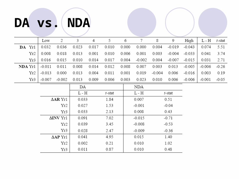
DA vs. NDA

Implications of DA and NDA

Discretionary component of accruals predict returns

Non-discretionary component of accruals do not predict returns

Evidence not consistent with extrapolation hypothesis

Earnings Components

Operating Performance

Accruals in the formation year significantly larger than earlier years.

Concurrent slow down of business?Working capital build up in expectation of higher

future sales?Declining sales turnover and earnings growth for

high accrual firms after portfolio formationExtreme accruals years mark a turning point in

the life cycle of firms

Conclusions

Accruals predict stock returnsChanges in inventory is the most important

component, which may not be consistent with delayed reaction hypothesis

Only discretionary accruals, but not nondiscretionary accruals, can predict future returns, thus disputing extrapolation bias hypothesis

High accruals years mark a turning point in operating performance, suggesting evidence of manipulating earnings

Roychowdhury (2006)

Managers manipulate real activities to avoid reporting annual losses.

Three real earnings manipulation activities are examined: Price discounts to temporarily increase sales Overproduction to report lower cost of goods sold Reduction of discretionary expenditures to improve reported

margins.

Cross-sectional analysis reveals that these activities are less prevalent in the presence of sophisticated investors.

Real earnings manipulations

real activities manipulation as departures from normal operational practices, motivated by managers’ desire to mislead at least some stakeholders into believing certain financial reporting goals have been met in the normal course of operations.

What is main difference between real and accrual based earnings manipulation? Real earnings manipulation differs from accruals

manipulation, which does not involves in direct cash flow consequences.

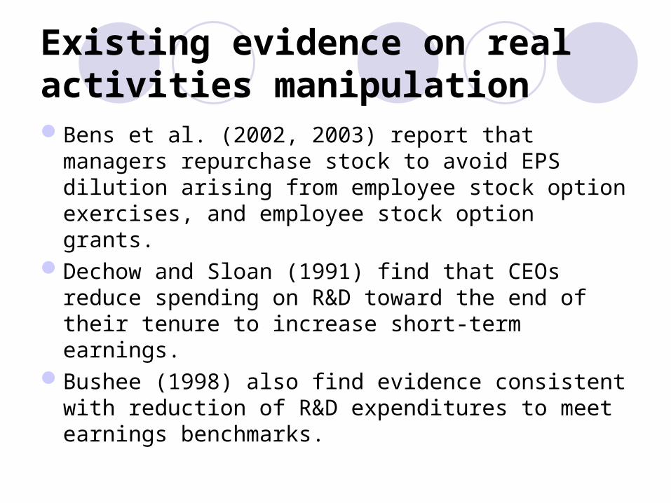
Existing evidence on real activities manipulationBens et al. (2002, 2003) report that managers

repurchase stock to avoid EPS dilution arising from employee stock option exercises, and employee stock option grants.

Dechow and Sloan (1991) find that CEOs reduce spending on R&D toward the end of their tenure to increase short-term earnings.

Bushee (1998) also find evidence consistent with reduction of R&D expenditures to meet earnings benchmarks.

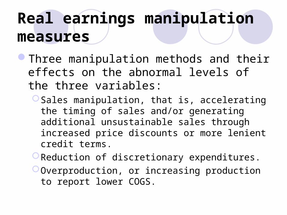
Real earnings manipulation measuresThree manipulation methods and their effects on

the abnormal levels of the three variables:Sales manipulation, that is, accelerating the timing of

sales and/or generating additional unsustainable sales through increased price discounts or more lenient credit terms.

Reduction of discretionary expenditures. Overproduction, or increasing production to report lower

COGS.

Sales manipulationSales manipulation as managers’ attempts to temporarily

increase sales during the year by offering price discounts or more lenient credit terms.

The increased sales volumes as a result of the discounts are likely to disappear when the firm re-establishes the old prices. The cash inflow per sale, net of discounts, from these additional sales is lower as margins decline.

Retailers and automobile manufacturers often offer lower interest rates (zero-percent financing) toward the end of their fiscal years.

In general, sales management activities to lead to lower current-period CFO and higher production costs than what is normal given the sales level.

Reduction of discretionary expendituresDiscretionary expenditures such as R&D, advertising,

and maintenance are generally expensed in the same period that they are incurred.

Hence firms can reduce reported expenses, and increase earnings, by reducing discretionary expenditures. This is most likely to occur when such expenditures do not generate immediate revenues and income.

Reducing such expenditures lowers cash outflows has a positive effect on abnormal CFO in the current period

Overproduction

To manage earnings upward, managers of manufacturing firms can produce more goods than necessary to meet expected demand. With higher production levels, fixed overhead costs are spread over a larger number of units, lowering fixed costs per unit. As long as the reduction in fixed costs per unit is not offset by any increase in marginal cost per unit, total cost per unit declines.

Nevertheless, the firm incurs production and holding costs on the over-produced items that are not recovered in the same period through sales. As a result, cash flows from operations are lower than normal given sales levels.

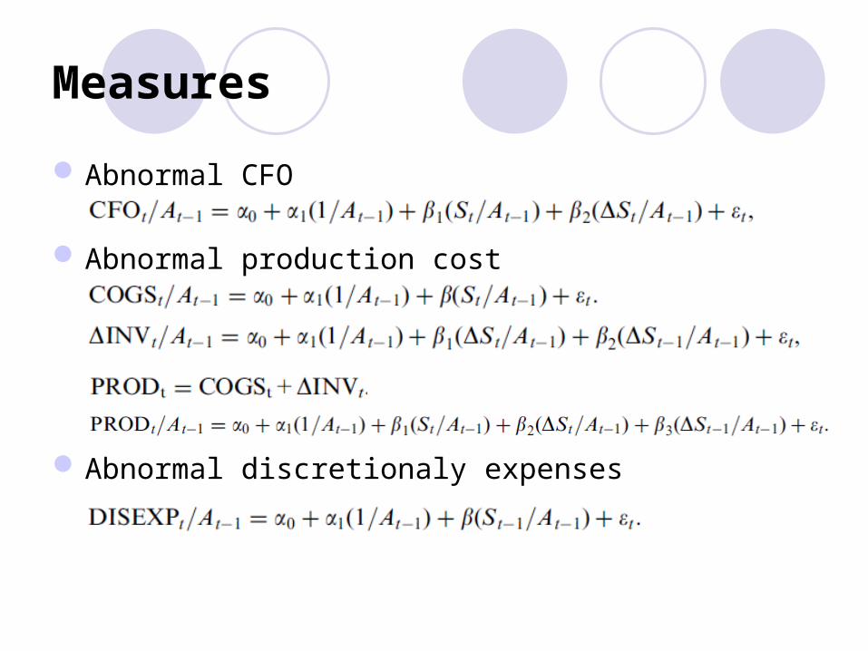
Measures

Abnormal CFO

Abnormal production cost

Abnormal discretionaly expenses

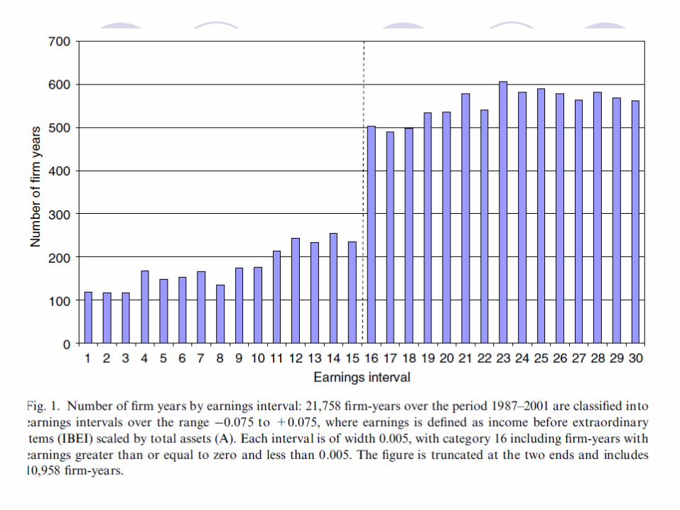
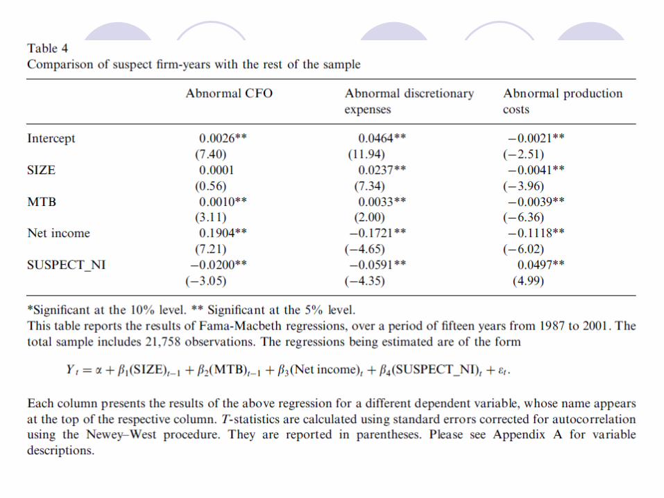
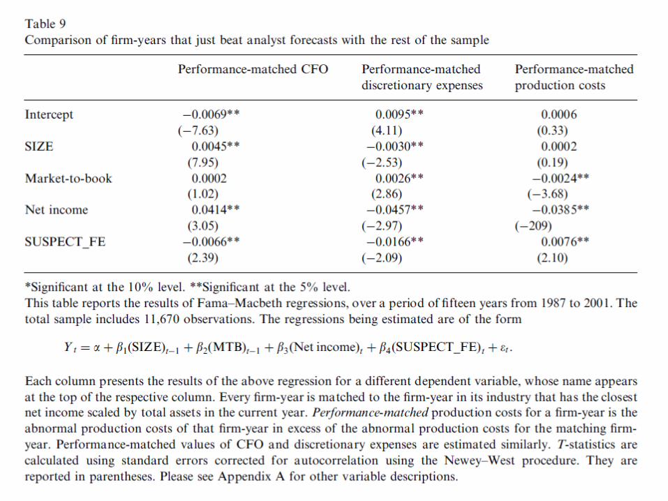
Interpretation

If firm-years that report profits just above zero undertake activities that adversely affect their CFO, then the abnormal CFO and abnormal discretionary expense for these firm-years should be negative compared to the rest of the sample.

Firm-years just right of zero have unusually high production costs as a percentage of sales levels.

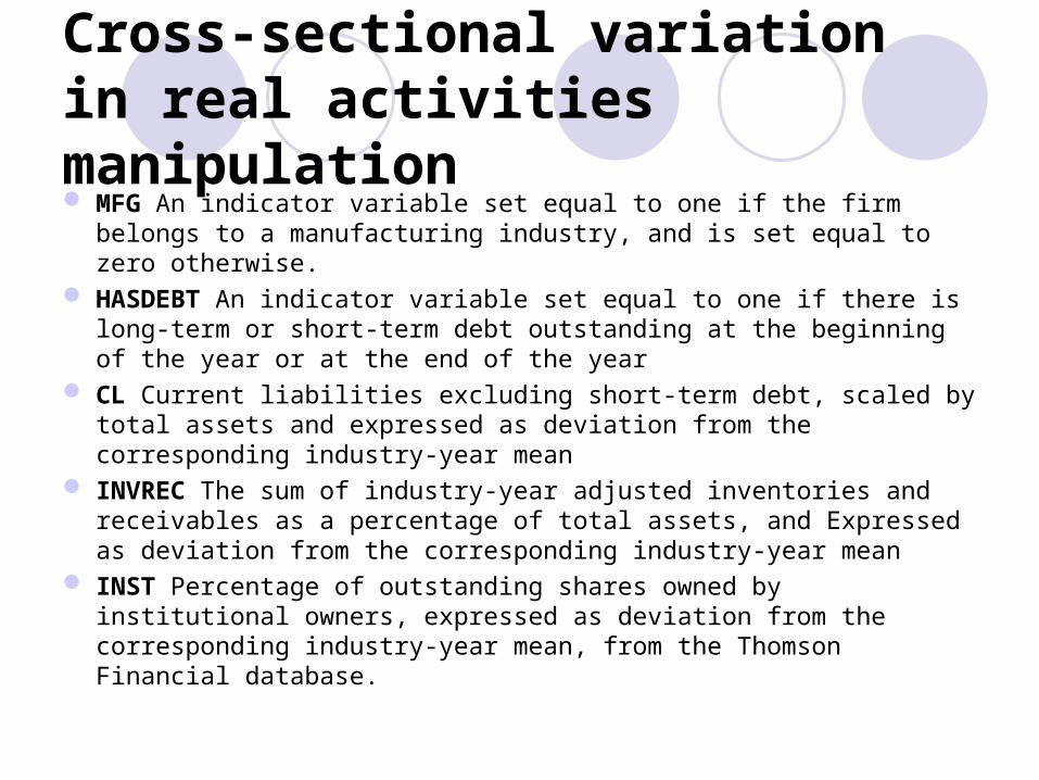
Cross-sectional variation in real activities manipulation MFG An indicator variable set equal to one if the firm belongs to a

manufacturing industry, and is set equal to zero otherwise. HASDEBT An indicator variable set equal to one if there is long-

term or short-term debt outstanding at the beginning of the year or at the end of the year

CL Current liabilities excluding short-term debt, scaled by total assets and expressed as deviation from the corresponding industry-year mean

INVREC The sum of industry-year adjusted inventories and receivables as a percentage of total assets, and Expressed as deviation from the corresponding industry-year mean

INST Percentage of outstanding shares owned by institutional owners, expressed as deviation from the corresponding industry-year mean, from the Thomson Financial database.

Cross-sectional variation in real activities manipulation