earnings responses to increases in payroll taxessaez/liebman-saezssa06.pdf · earnings responses to...

Earnings Responses to Increases in Payroll Taxes

Jeffrey Liebman, Harvard University and NBER Emmanuel Saez, University of California, Berkeley and NBER

September 2006

Abstract

This paper uses SIPP data matched to longitudinal uncapped earnings records from the Social Security Administration for 1981 to 1999 in order to analyze the earnings responses to increases in tax rates and inform discussions about the likely effects of raising the Social Security taxable maximum. The earnings distribution of workers around the current taxable maximum is inconsistent with an annual model in which people are highly responsive to the payroll tax rate, even in the subset of self-employed individuals. Panel data on high-earnings married men display a tremendous increase in earnings over the 1980s and 1990s relative to other groups with no clear breaks around the key tax reforms. This suggests that other income groups cannot serve as a control group for the high earners. Our analysis does not support the finding of a large behavioral response to taxation by wives of high earners. We actually find a decrease in the labor supply of wives of high earners around both the 1986 and the 1993 tax reforms, which we attribute to an income effect due to the surge in primary earnings at the top. Policy simulations suggest that with an earnings elasticity of 0.5, lost income tax revenue and increased deadweight loss would swamp any benefits from the increase in payroll tax revenue. In contrast, with an elasticity of 0.2, the ratio of the gain in OASDI revenue to lost income tax revenue and deadweight loss would be much greater.

This research was supported by the U.S. Social Security Administration through grant #10-P-98363-1-01 to the National Bureau of Economic Research as part of the SSA Retirement Research Consortium. The research in this paper was conducted while Liebman was a Special Sworn Status researcher of the U.S. Census Bureau at the Boston Census Research Data Center (BRDC). This paper has been screened to insure that no confidential data are revealed. The findings and conclusions expressed are solely those of the authors and do not necessarily represent the views of SSA, the Census Bureau, any other agency of the Federal Government, or the NBER. Support for the Census research data centers from the NSF (award no. ITR-0427889) is gratefully acknowledged. We thank Erin Metcalf, Daniel Ramsey, and Sarena Goodman for excellent research assistance. We thank Leora Friedberg for helpful comments and discussions.

1

1. Introduction

A 12.4 percent Old Age Survivors and Disability Insurance (OASDI) payroll tax

is assessed on the first $94,200 of a U.S. worker’s earnings.1 Earnings above $94,200 are

exempt from this tax. This exemption means that only 86 percent of earnings by workers

who are covered by Social Security are currently subject to OASDI payroll taxes, and this

fraction is expected to fall to under 85 percent by the end of the decade.2 When the

Social Security payroll tax was first introduced in 1937, ninety-two percent of covered

earnings were taxable. This level has fluctuated over time, reaching a low of 71 percent

in 1965. The 1977 amendments to the Social Security Act restored the level to 90

percent, but the level has eroded over the past 25 years as earnings growth among high

earners has exceeded that of other workers. Moreover, although wages as a percentage of

total compensation have remained fairly steady in recent years at around 90 percent, there

is concern that if health cost growth continues to exceed GDP growth, the share of non-

wage compensation will rise, reducing the Social Security wage base relative to total

compensation.

Among the policy options for closing the long-run gap between Social Security

expenditures and revenues is to increase the share of covered earnings that is subject to

the OASDI payroll tax. For example, legislation introduced several years ago by

Senators Moynihan and Kerrey would have increased the maximum level of earnings

subject to taxation so that 87 percent of earnings would be covered by Social Security.

Later, legislation introduced by Senator Moynihan alone would have raised the limit to

90 percent of earnings. Former President Clinton carefully ruled out raising the payroll

tax rate but not the tax base. Plan 3 of President Bush’s Commission to Strengthen

Social Security originally envisioned raising the maximum taxable earnings level to

cover 90 percent of earnings, though in the final report this provision was replaced by a

general revenue transfer from an unspecified source that was described in a footnote as

equaling the amount of revenue that would be gained from increasing the maximum

1 This is the 2006 maximum. The amount is adjusted annually based on the growth rate of average wages.2 Only 5.5 percent of covered workers have earnings above the maximum taxable level. These numbers are preliminary data for 2003 from the 2005 Annual Statistical Supplement to the Social Security Bulletin.

2

taxable earnings level. Still other experts have suggested that the cap on taxable earnings

be removed altogether as was done for the Medicare payroll tax in 1993.3

Although public finance economists generally prefer base-broadening to tax-rate

increases as a way to increase revenue (since deadweight loss rises in proportion to the

square of the tax rate but only linearly with the tax base), some have argued that raising

the payroll tax base would be a particularly inefficient way to raise additional revenue for

Social Security (Feldstein, 2004). This argument relies on recent research by Feldstein

(1995), Eissa (1995), Auten and Carroll (1999), and Gruber and Saez (2002) that has

shown that high-income taxpayers are more sensitive to taxation than lower income

taxpayers. Those opposing an increase in the taxable maximum have argued that the high

elasticities estimated in these papers imply that focusing a 12.4 percentage point tax

increase only on high earners (with high pre-existing tax rates) would produce mostly

deadweight loss and raise relatively little revenue. Moreover, they argue that for the

government as a whole, some or all of the increased OASDI revenue would be offset by a

decline in Medicare and income tax revenue.

There are, however, several reasons why this result is far from certain. First, for

increases in the maximum taxable earnings level that do not eliminate the cap altogether,

there may still be a substantial number of taxpayers – those with earnings above the new

limit – for whom the tax increase will be inframarginal. In other words their marginal tax

rate will not change, and there will be no efficiency effects on those taxpayers (indeed,

we might observe an increase in their earnings due to the income effect). Thus,

determining the impact of a particular policy requires careful simulation of the responses

of both taxpayers between the old and new tax thresholds and those above the new tax

threshold. Second, most of the evidence suggesting large elasticities for high-income

taxpayers has used tax return data and focused on broad income measures such as

adjusted gross income (AGI) or taxable income. Because there are more opportunities to

manipulate AGI or taxable income through asset transactions, taking deductions, and

noncompliance than there are for earnings (and because even the standard and itemized

deductions mechanically exclude some earnings from income taxation), the elasticity

estimates for high earners for these broader measures of income are not directly relevant

3 See Diamond and Orszag (2005) for discussion of some such options.

3

for studying the response of the wage base to changes in the Social Security tax base.

Indeed, Gruber and Saez find that even when shifting from taxable income to AGI as an

income measure average elasticities fall from 0.45 to around 0.15. One would expect

average earnings elasticities to be even lower. Third, tax-return based studies are forced

to aggregate the earnings of husbands and wives since these are reported together on the

income tax return. However, there is good evidence that labor supply elasticities differ

for men and women (Mroz 1987, Eissa 1995), and a careful analysis of responses to

changes in the Social Security tax base would need to take these differences into account;

in particular married women make up a relatively small fraction of workers with earnings

levels above the current taxable maximum.

In this paper, we provide new evidence on the earnings response to taxes using a

special version of the Survey of Income and Program Participation (SIPP) that has been

matched to administrative earnings records from the Social Security Administration. We

show that the distribution of taxpayers around the taxable maximum is quite smooth –

and is therefore inconsistent with a high degree of earnings responsiveness to taxes under

the standard one-period labor supply model with fully-informed individuals and no

uncertainty. This is true for the entire population as well as for the self-employed – a

group that presumably has a higher-than-average amount of control over their earnings

levels. We also examine the earnings behavior of taxpayers at different points in the

income distribution around the time of the 1986 tax reform (which reduced marginal tax

rates for high earners) and the 1993 tax reform (which increased marginal tax rates for

high earners). For men we find that the pre-existing trends for very high earners were

quite different than those for even slightly-lower earners and that there is no evidence of

a break in these trends around the tax reforms. We also revisit the famous, but never-

published, findings of Eissa (1995) regarding women married to high earners. Our

results suggest that there is little empirical support for the proposition that women

married to high earners altered their labor supply behavior in response to the major tax

changes in recent decades.

4

2. Background

Until about 15 years ago, the conventional wisdom was that people’s incomes

were largely unresponsive to taxation. Empirical studies of the responsiveness of hours

worked to marginal tax rates found elasticities very close to zero, particularly for prime-

age males. While there was greater uncertainly about estimates for females – with some

evidence of an extensive-margin response (Mroz 1987, Hausman 1981) --, and there were

some structural models such as those by Hausman (1981) that suggested large

compensated elasticities, the bulk of the evidence suggested small amounts of deadweight

loss from taxation.

In recent years, a new view has emerged. This new view is based on the insight

that workers can respond to taxes by changing their behavior in many ways –not simply

by varying their hours worked. For example, workers can alter the intensity of their work

effort per hour, their risk taking, their compliance behavior, the composition of their

compensation between untaxed fringe benefits and taxable monetary pay, the split

between compensation that is taxed as labor income and compensation taxed as capital

income, and their itemized deductions. All of these behavioral responses contribute to

the distortionary effects of taxation and can be analyzed by studying how taxable income

responds to tax rates (Feldstein, 1999).5

This theoretical insight coincided with the emergence of a new empirical

approach to measuring behavioral responsiveness to taxation – using tax reforms as

natural experiments. If taxpayers understand how their budget constraints are changing

and can alter their behavior within a few years of a change in tax laws, then it is possible

to measure the behavioral response to taxation by comparing outcomes before and after

the change in tax laws. Since other features of the economy are always changing, this

methodology, applied first in Lindsey (1987), generally requires a control group – a set of

taxpayers who are similar to the ones affected by the tax change but who were not

affected by it. There are four key empirical studies upon which the new view is built.

Feldstein (1995) analyzed panel tax return data and showed that the reported incomes of

the 57 very-high-income married couples in his data set increased much faster than the

5 Slemrod (1995) raises an important issue which we ignore in our analysis – that behavioral

responsiveness on one margin will likely depend on what other margins are available to respond along.

5

reported incomes of lower-income taxpayers from 1985 to 1988. He attributed this

differential increase to the Tax Reform Act of 1986 which lowered marginal tax rates

much more at the very top than at other points in the income distributution and estimated

very large elasticities of reported incomes with respect of the net-of-tax rate (between 1

and 3). Auten and Carroll (1999) replicated the Feldstein study using a much larger panel

of tax returns available at the U.S. Treasury and estimated taxable income elasticities

around 0.6. Eissa (1995) showed, using CPS repeated cross-section data, that women

married to very high income husbands increased their labor supply along both the

extensive and intensive margins, relative to women married to middle-high income

husbands between 1983-1985 and 1989-1991. She also attributes those patterns to the

Tax Reform Act of 1986 where women married to very high income husbands

experienced large marginal tax rate reductions relative to other married women. She finds

labor supply elasticities for married women around one. Gruber and Saez (2002) use

panel tax return data from 1979 to 1990 and study the behavioral response to the entire

set of tax changes that occurred in the 1980s . They find that elasticities for high-income

taxpayers are higher than those for lower income taxpayers and that the elasticity of

taxable income is larger than the elasticity of income before deductions.

These findings have been challenged on several grounds. First, the samples of

very high income taxpayers used in several of these papers were quite small. Feldstien

(1995) does not present any standard errors for his estimates and the 95 percent

confidential intervals for Eissa’s (1995) elasticity estimates include zero. Second, some

have questioned whether samples of lower-income taxpayers can serve as adequate

control groups for higher income taxpayers (Goolsbee, 2002). Very high income

taxpayers have different income sources that respond differently to economic conditions.

Rising income inequality has meant that the incomes of very high income taxpayers have

been rising much more rapidly than the incomes of those who are even slightly lower in

the income distribution, and these trends are not adequately controlled for in most of the

natural experiment studies. And very high income taxpayers are more likely to shift

6

income across years in response to tax reforms in ways that can lead natural experiment

studies to confuse short-term timing shifts with permanent responses. Tax reforms may

also prompt behavioral changes that shift income between the corporate income tax and

the personal income tax. Studies that look only at the personal income tax system can

confuse this shift with a permanent change in revenue levels (Slemrod, 1995). Slemrod

(1998) and Saez (2004) provide summaries of this literature and of these identification

issues.

Moreover, for the question at hand, most of these results, even if internally valid,

are not directly applicable. Three of the four studies described above focus primarily on

taxable income. As was mentioned before, taxable income responses are likely to be

larger because there are more margins that can be adjusted than is possible with earnings.

The only one of these studies that focuses on earnings focuses on married women, a

group that we will see shortly makes up a very small fraction of the high earners who

would experience increases in marginal tax rates if the social security maximum taxable

earnings level were raised. Thus there is need for direct empirical evidence on earnings.7

3. Data

To study the earnings behavior of taxpayers at and above the current Social

Security taxable maximum, one needs uncapped earnings data from a large sample of the

population. Standard survey data sets such as the CPS are not ideal for this purpose

because they top code data on high earners and contain measurement error. Standard tax-

return based samples are also of limited use for this kind of study because the earnings of

both spouses in married couples are usually aggregated together on the wage and salary

line of the tax form, whereas the OASDI payroll tax applies to each spouse individually.

Finally, a panel data set is strongly preferred for studying behavioral responses to tax

reforms because in repeated cross-section analyses the composition of taxpayers in the

different income groups can change over time in ways that may bias estimates.

7 Other studies (Gentry and Hubbard 2004, Goolsbee 2006) have specifically analyzed the effects of taxes

on entrepreneurship, which in some cases can correspond with the self-employment component of OASDI

earnings.

7

For this study we make use of a special data set that has been created via

cooperation between the Census Bureau, the Social Security Administration, and the

Internal Revenue Service. The data set matches many of the panels from the Survey of

Income and Program Participation to administrative earnings records. Originally, the

SIPP was matched to the Social Security Administration’s summary earnings file which

contains only earnings up to the taxable maximum in each year. However, in the past

few years it has been possible for researchers who are special sworn Census Bureau

employees to work with the SIPP matched to the raw uncapped wage and salary

information from a worker’s W2 along with measures of self-employment earnings

originating from the worker’s tax return.

The data we use consist of the 1984, 1990, 1991, 1992, 1993, and 1996 SIPPs

which have been matched to uncapped earnings data that extend from 1981 to 1999.

Roughly 86 percent of SIPP sample members can be successfully matched to earnings

records. We reweight the successfully-matched portion of the SIPP samples to represent

the full sample – by adding a component to the standard SIPP weights that comes from

regressing the probability of being a successful match conditional on SIPP observables.

Further details on the match procedure are in an appendix that is available from the

authors.

We can explore whether the SIPP-matched sample is representative of the overall

population of administrative earnings records by comparing the administrative earnings

distribution in our sample to published distributions from the Social Security

administration. Appendix Figure 1 shows that there are more individuals with earnings

below $20,000 in the published SSA tables than in our data set. We do not have a good

explanation for why the SIPP-SSA match has too few low earners, though one of us

found a similar pattern in matching the CPS to tax return data (Liebman, 1996). Further

analysis (not shown) reveals that we match the published distribution much more closely

at the higher earnings levels that are the focus of this study.

Table 1 shows some simple descriptive statistics for workers at different points in

the earnings distribution using the 1996 SIPP panel and the 1996 administrative earnings

data (this is an appealing subset of the data to use since it is the latest year for which the

survey date and the date of the administrative data correspond). The top row of the table

8

shows that average earnings in the administrative records for workers with earnings

below the 1996 taxable maximum of $62,700 were $16,051. Average earnings for those

between the taxable maximum and the level that would result in 90% of covered earnings

being taxed was $71,869. Finally the average earnings of those above the 90% of

covered earnings level was $172,239. The next two rows of the table decompose these

earnings into wage and self-employment earnings. For those below the taxable

maximum, self-employment earnings made up 4.2 percent of total earnings; for those in

the middle group, self-employment earnings were 6.4 percent of earnings, and for those

in the top group they were 14.9 percent of earnings. The share of workers with any self-

employed earnings shows a similar pattern. 7.4 percent of the lowest group, 13 percent

of the middle group, and 23.8 of workers in the top group had self-employment earnings

(often in conjunction with wage earnings). The mean age was a bit higher in the higher

earnings groups than in the lower-earnings group. But the share of earners who were

over 54 – an age group whose retirement decisions could be affected by tax rates -- was

lower in the two high-earnings groups than in the lower-earning group

The gender and marital status patterns vary considerably across groups. Only

31.3 percent of workers in the low-earning group were married males, compared with 68

percent of the group between the taxable maximum and 90 percent of covered earnings

and 79 percent of those in the top group. In contrast, the share of married females and of

unmarried males and females is much lower in the groups that would be directly affected

by an increase in the taxable maximum. Taken as a whole, these descriptive statistics

suggest that the bulk (almost 70 percent) of those who would see their marginal tax rate

increase if the taxable maximum were raised are prime-age married – a group that is

generally thought to have low earnings responsiveness to taxation. However, the large

number of self-employed workers and the non-trivial fraction of married females might

be expected to have greater responsiveness.

4. The Distribution of Earnings around the Current Taxable Maximum

Standard economic theory makes strong predictions about the location of workers

in relationship to kinks in the tax schedule. At a kink point where marginal tax rates

increase with earnings levels, we should observe a bunching of earnings just at or below

9

the kink.8 For a kink, like that produced by the social security taxable maximum, where

marginal tax rates fall, there should be a gap in the earnings distribution. This gap should

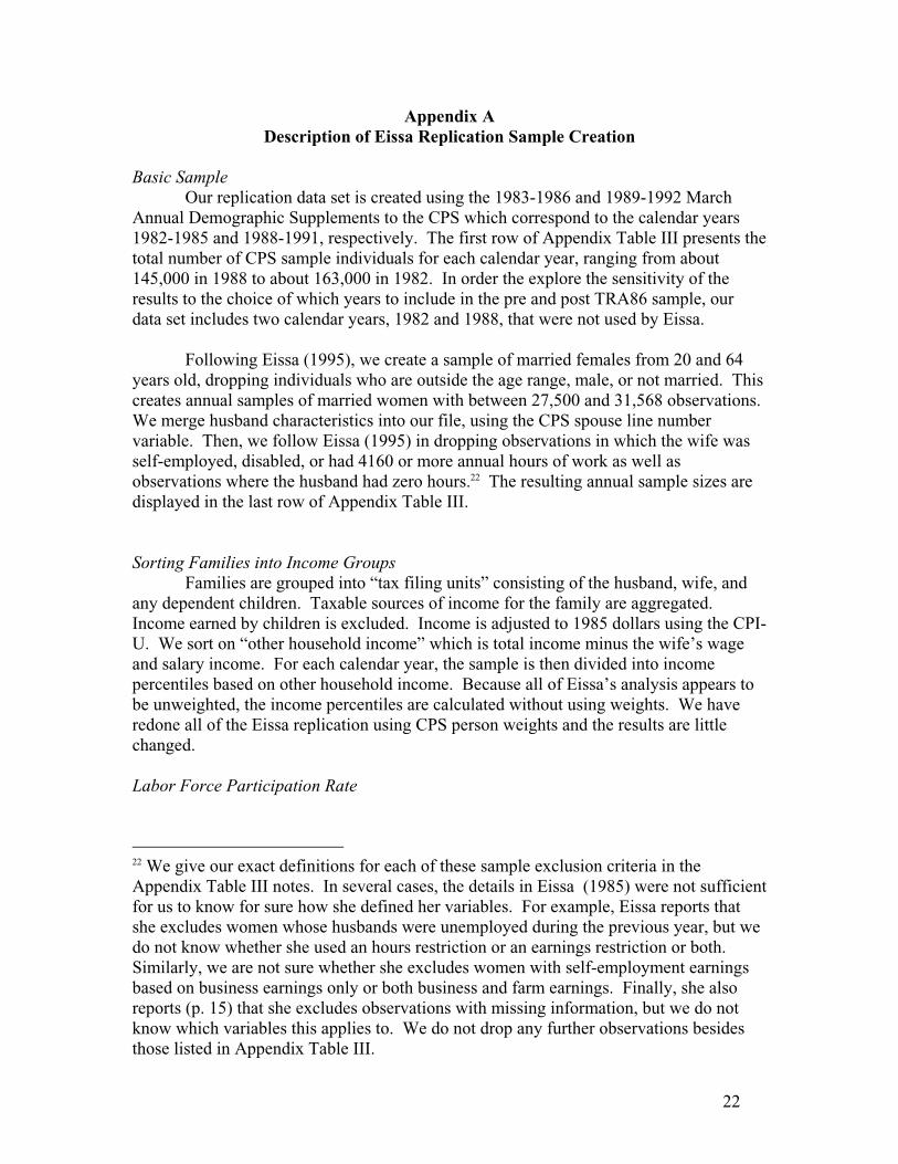
be visible even with relatively low responsiveness to taxation. The top panel of figure 1

shows the gap that would occur under the standard model if the earnings elasticity were

0.20.9 The bottom panel of figure 1 shows the actual distribution of earnings around the

taxable maximum. There is no gap whatsoever. Figure 2 takes our full data set of

earnings from 1991-1998 and plots earnings relative to each year all combined on a

single figure so as to smooth out the noise that was present in the 1996 figure because of

the moderate sample size.10 The distribution is completely smooth around the kink point.

Indeed, for this graph to arise under the standard model, the implied distribution of

earnings without the tax variation would require a big hump in earnings around the

taxable maximum, something that is clearly implausible. Figure 3 shows that even

among the self-employed – who are generally though to have substantial control over

their earnings -- there is no gap in the earnings distribution at the taxable maximum.

These pictures are very difficult to reconcile with the model underlying the

natural experiment evidence suggesting high elasticities – that people are aware of

marginal tax rates and are able to respond relatively quickly to them. Instead, they

suggest that people are unresponsive to the marginal tax rates implicit in the payroll tax –

and certainly unresponsive to the exact location of the taxable maximum (which of

course would be the key question if the threshold were raised to say 90 percent of

8 Liebman (1998) studies bunching around the kinks generated by the EITC and finds no evidence of

bunching. Saez (2002) studies bunching around kink points of the federal tax schedule. He does not find

evidence of bunching except for the self-employed around the first kink point of the EITC. The one place

where there is a clear evidence of bunching for wage earners is around the kink created by the Social

Security retirement earnings test (see Friedberg, 2000 and Burtless and Moffitt, 1984). 9 This figure is created by assuming that preferences are quasilinear with U=WL(1-t)-[L^(1+k)]/(1+k) and a

constant tax rate and then inverting the first order condition to uncover the (smooth) wage distribution.

Then with the smooth wage distribution we simulate behavior under the actual nonlinear tax schedule. 10 We restrict the figure to 1991-1998 because our self-employment data are the amounts subject to the

Social Security and Medicare tax and are therefore available above the taxable maximum only after the

Medicare cap was raised in 1991 to $125,000 (it was completely eliminated in 1994).

10

earnings). If this is true, the deadweight loss associated with an increase in the taxable

maximum could be negligible.

It is possible to come up with models in which people’s behavior is distorted by

the taxable maximum, yet they do not avoid earnings levels around the kink point. One

possibility is that a portion of earnings are random so that people cannot optimize

perfectly. The potential importance of this explanation depends on the share of the year-

to-year variation in earnings that is unpredictable. Another possibility is that people

have little short-term (say under 10 years) control over their earnings levels. However,

this assumption would undermine the natural experiment studies of tax reforms (as would

the assumption that people are solving a complicated lifetime dynamic problem when

making their labor supply decisions – and stopping at a point that is suboptimal in a static

model on the way to some other location). Liebman and Zeckhauser (2005) propose an

alternative explanation – that some people misperceive tax schedules in systematic ways

while other people are rational but have considerable uncertainty about the location of

kink points in the tax schedule. These sorts of models can explain the lack of the gap in

this model but tend in the direction of people responding to average tax rates rather than

marginal tax rates – which Liebman and Zeckhauser show implies that optimal tax rates

on high earners should be much higher than under the standard assumption that people

respond to marginal tax rates.

5. Earnings Responses to Tax Reforms

A second methodology for examining the sensitivity of earnings to marginal tax

rates is to compare earnings levels before and after a change in marginal tax rates. The

ideal change to study would be a change in OASDI payroll tax rates. Unfortunately,

annual changes in the OASDI contribution rates and in the maximum taxable earnings

levels have been too small and gradual to allow such an investigation. Instead, we study

the earnings response to two broader tax reforms: the Tax Reform Act of 1986 (TRA86)

and the Omnibus Budget Reconciliation Act of 1993 (OBRA 1993). TRA86 cut

marginal federal income tax rates for very high earners from 50 percent to 28 percent.

OBRA93 raised marginal tax rates for high earners by 10.9 percentage points (the top

income tax rate was increased from 31 to 39.6 percent and the cap on HI taxes was

11

removed, making the top rate effectively 41.9 percent).11 While there have been

numerous studies that have studied the response of broader income categories such as

AGI and taxable income to these tax reforms, there is little work that has focused on the

earnings response, other than Eissa’s work on the wives of high earners.

For each tax reform, we pool all of the six SIPP panels that we have access to and

construct a panel data set of married couples. Our intention is to analyze a sample of

married couples who were continuously married during our analysis period.12 For our

TRA86 analysis, we use the SIPP retrospective marital status history topical modules to

determine whether people in the 1990, 1991, 1992, 1993, and 1996 SIPP panels were

continuously married back to the beginning of our analysis period (1981). For our

OBRA93 analysis we include people who were continuously married back to 1988. In

both analyses, we include all married couples from the 1984 SIPP panel since we cannot

observe martial status beyond the end of the SIPP survey period.13 We further restrict the

sample to those between the ages of 21 and 56 in the year of the tax reform (1986 or

1993) so that retirement choices do not dominate the analysis.

Table 2 shows some descriptive statistics for the 1986 tax reform sample (similar

statistics for the 1993 sample are in table 5). To study the behavior of the very high

income groups who were affected by the tax changes, we divide the sample into six

income groups following Eissa (1995), and use various of the lower-income groups as

control groups in studying the behavior of the highest income group. Our groups are

formed by ranking households based on husband’s average earnings between 1983 and

1989.14 We average over both the pre-reform and post-reform period to minimize the

mean-reversion bias that would occur if one ranked households only on pre-reform

earnings. The three groups shown in table 2 are the three that were studied by Eissa

(1995). The 75th percentile group consist of those with average husband’s earnings

11 The effective rate is (0.396+0.029)/(1+0.0145)=41.9% as the federal income tax rate does not apply to employer HI payroll contributions. 12 Feldstein (1995) and Gruber and Saez (2002) similarly focus on taxpayers with no marital status

changes. 13 Our results are insensitive to dropping the 1984 panel. 14 Note that unlike Eissa (1995) we rank only on husband’s earnings, not on husband’s earnings plus the limited components of asset income measured by the CPS. Relative to Eissa, our approach has the advantage that it is based on administratively measured data that is not top coded and on panel data rather than repeated cross sections, but it has the disadvantage that it does not include any asset income.

12

between the 75th and 80th h percentile. The 90th percentile consists of those between the

90th and 95th percentile, and the 99th consists of those above the 99th percentile.

Notice that the 99th percentile sample size is only 250 (and is about one-fifth as

large as the other two groups). Thus, even when pooling the 209,000 individuals in the

six SIPP panels, the restriction to continuously married couples and very high earners

produces a fairly small sample. Notice also the four rows at the bottom of the table

which show the average earnings of husbands in different groupings of pre-reform and

post-reform years. In the 75th percentile sample, average earnings rose by about 10

percent from the pre-TRA86 period to the post-TRA86 period. In the 90th percentile

sample, earnings rose by 15 to 20 percent. In the 99th percentile sample, earnings almost

doubled. So either tax policy had an extraordinary effect on the high earners or the other

things going on in the economy (including possibly different age-earnings profiles for

very high earners) made the experience of the high-earnings group very different than

that of the other groups.15

Figure 4 shows that the latter is almost certainly the case. This figure shows the

change in the mean earnings of married men relative to 1981 for our six earnings groups.

The top panel shows the increase in dollars. Because the large increase in the top group

makes it hard to see the changes for the lower-income groups, the bottom panel shows the

increase for each group relative to that group’s 1981 earnings level using a logarithmic

scale. From the figure we can see that over the 1981-1991 period, average earnings of

the married men in the highest earnings group grew by $200,000. Average earnings for

this group was about $100,000 at the beginning of this period, so the gain was a 200%

increase. In contrast the 90th percentile group experienced only at 50 percent increase

over this period and earnings for the bottom 80 percent hardly increased at all. The

increase over this period for the highest earnings group was steady and shows no break in

the trend around the time of TRA86. We draw several conclusions from these data.

First, there is nothing in these data that would lead one to believe that taxes were a major

part of the story for the increase in earnings among high earners. Second, since the

underlying trend is so large and varies so dramatically across the income groups, it is

15 Saez (2004) points out that it is difficult to attribute the full increase of top incomes since the 1980s to

tax changes only.

13

impossible to know what the counterfactual trend would have been in the absence of

TRA86 – and to rule in or out a tax effect. Third, it seems almost ludicrous to imagine

that taxpayers in the 75th percentile group of even 90th percentile group could be an

adequate control group for the 99th percentile high-earner group.16

Figures 5 and 6 show the corresponding trends for the wives of the husbands we

observed in Figure 4. Figure 5 shows the change relative to 1981 in the fraction of wives

with positive annual earnings. Figure 6 shows the average earnings (including zeros) of

the wives. In the first of these figures we see that there was a large drop in the annual

labor force participation of 99th percentile wives starting in 1987 – just after TRA86.

This is the opposite of the Eissa (1995) finding.17 Notice that annual labor force

participation rates are flat for the 90th and 95th percentile groups and rising for the three

other groups. Thus, this behavior of the very high income wives seems to be

fundamentally different than that of the other groups. We think the most likely story is

an income effect. Given that their husband’s earnings are tripling over this period it is

not surprising that some of the 99th percentile wives left the labor force. In figure 6 we

see that the pattern of earnings for wives married to high earners is also quite different

from that of the other groups, both in its underlying trend and in the change before and

after 1986. For the 99th percentile wives, earnings are flat. For the other five groups they

are rising steadily.

Tables 3 and 4 show when performing Eissa-style difference-in-differences

regressions, the differences between the 99th percentile and the other groups in their

before and after TRA86 outcomes are statistically significant. For each table we present

16 Note that Eissa was probably unaware of the extent to which the high-earner husbands differed in their

income growth from the other groups because the CPS is top-coded -- so the growth in earnings was not

observable in her data set. Appendix Table IV shows that almost two-thirds of the households in Eissa’s

99th percentile sample were affected by top coding. Appendix Figure 4 shows that because of this top

coding Eissa’s income family income measure was constant in real dollars over this time period for the

high income groups. 17 A significant fraction of the wives leaving the labor force were earning less than $2500 in the pre-TRA86

period. When people with less than $2500 of earnings are dropped from the analysis there is still a drop in

earnings but the figure appears smooth and continuous.

14

this result in 16 different ways to show whether or not the results are sensitive to

alternative specifications. We present results relative to the two control groups (90th

percentile and 75th percentile) used by Eissa. We present results with and without age

covariates. Finally we show results for two different definitions of the pre-TRA period

and two different definitions of the post-TRA period. We draw three conclusions from

our analysis of the data on wives. First, the underlying trends before TRA86 for the

different income groups are so different that it seems unlikely that any lower income

group could serve as an adequate control group for the 99th percentile group. Second,

because the husband’s earnings were changing so dramatically for the 99th income group,

other groups would not be adequate control groups even if the pre-TRA86 trends in

female labor force behavior had been similar. Third, when one uses a panel data set with

high quality administrative earnings records one finds statistically significant negative

“effects” of TRA86 – the opposite of the (not statistically significant) Eissa finding.

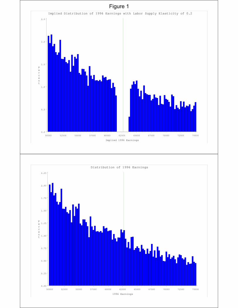
Figures 7, 8, and 9 repeat this analysis for the OBRA 1993 sample. This sample

differs from the TRA86 sample in that the income groups are formed based on average

1990 to 1998 earnings rather than 1983 to 1989 earnings. In addition, consecutive years

of marriage are required only back to 1988, not back to 1981. The basic trends are

similar to those in the earlier sample. First, the earnings of the 99th percentile husbands

are increasing much more rapidly than those in the other groups. Second, relative to the

other groups, over the entire sample period the annual labor force participation of the

wives of the very high-earners is falling. However, this flattens out in the aftermath of

the increase in marginal tax rates imposed in OBRA93, resulting in estimates that are

very near zero for the difference-in-difference regressions in Table 6. Again, this is

counter to what would be expected from the change in marginal tax rates. The trend

decline in labor force participation among wives of high earners should accelerate in

response to the increase in marginal tax rates, not disappear. Third, average earnings

pick up after OBRA93 for the wives of high earners -- again this result, though

statistically insignificant, is the opposite of what would be predicted if the tax change

were the main factor explaining changes over time in the earnings behavior of married

women.

15

6. Replicating the Eissa Results in the CPS

Because our results are directly at odds with the Eissa (1995) result, we set out to

see if we could replicate her results using the same data and methodology that she used

and determine why our results with the SIPP-SSA matched data differed from hers.

Appendix tables I and II show that while we could not replicate her samples exactly, we

match her basic results and summary statistics by income groups quite closely.18 Note

that her per-year samples of women in the high-income group are quite similar to the size

of our SIPP samples – a bit over 225 per year. Standard errors are similar in the two sets

of analyses – the reason why our TRA86 results are statistically significant and hers (in

the opposite direction) are not is simply that our estimated impact is about twice as large.

Figure 10 shows the main findings from our reanalysis of the CPS data. It shows

the fraction of women with positive annual earnings in each of the income groups based

upon husband earnings and other (primarily asset) income. Women in the lowest income

groups have the highest rates of labor force participation, so going from top to bottom the

lines show the under 75th percentile group, the 75 th to 80th percentile group, the 80th to

90th group, the 90th to 95th group, the 95th to 99th group, and the over 99th percentile

group.

It is clear that the CPS estimates of labor force participation for the 99th percentile

group are very imprecise -- with the estimates fluctuating by any much as 10 percentage

points from year to year. It is also clear that all of the groups had pre-existing upward

trends in the early 1980s, trends that leveled off to various degrees around 1988. Thus

any difference-in-differences comparison across these groups will represent some

combination of differential underlying trends, different timing and degree of when the

trends leveled off, and noise associated with sampling variation. Identifying effects of

tax policy in this kind of environment will be quite challenging. In particular, Eissa-style

difference-in-differences estimates will be quite sensitive to whether 1988 (an unusually

low year for the 99th percentile group) is included as a post-TRA86 year or whether,

instead, the post-TRA86 period is considered to begin in 1989 and therefore extends to

include 1991 (an unusually high year). Eissa argues that it should begin in 1989 because

18 Appendix A describes in detail our construction of our sample used for replicating the Eissa results.

16

some provisions in TRA86 were still being phased-in in 1988. Feldstein (1995) however

conducts his TRA86 study comparing 1988 to 1985, as 1988 was the first year in which

the top marginal rate was 28 percent. Table 8 illustrates more precisely the sensitivity of

the results to choice of which TRA86 years are included. In specifications in which the

post-TRA86 period starts in 1989 and includes 1991 there are, consistent with Eissa

(1995), positive results. However, when the post-TRA86 period starts in 1988 and

excludes 1991, the estimated impact is essentially zero. Table 9 shows that a similar

pattern holds for earnings.

What happens when we apply Eissa’s CPS-based methodology to OBRA 1993?

In Figure 10, one can see that although labor force participation rates for the 99th

percentile group are fluctuating widely, they are essentially flat from 1989 on. In

contrast, labor force participation rates for wives in the 75th percentile and 90th percentile

groups are continuing to rise. Difference-in-differences regressions will therefore show a

decline for the high earners relative to the lower earners – consistent with what we saw in

the SIPP-SSA match (figure 8). In this period, this result is also consistent with what

would be predicted from the OBRA93 increase in marginal tax rates. In Tables 10 and

11, we show that the results for annual labor force participation are large and (for the 95th

-90th comparison) often statistically significant, while the ones for earnings are not large

enough to be statistically significant.

It is interesting to note that if one had simply set out to replicate the Eissa (1995)

methodology for OBRA 1993 using the CPS and not examined the underlying trends

more closely, one would have concluded that her results were strongly confirmed. A tax

change for high earners in the opposite direction of the TRA86 reform had large effects

on the labor supply of high-income wives -- in the direction predicted by the change in

marginal tax rates. Under the assumption that the underlying trends that could not be

sufficiently controlled for were similar (and in the same direction) in the two time periods

this would be pretty strong confirmation.

We, however, come to a very different conclusion. First, we think we have

established that none of the lower–earning groups are plausible control groups for the 99th

percentile group. Second, we think the small samples of high earners are too noisy to

draw any strong conclusions – results are sensitive to small changes in specification.

17

Third, we think the balance of the evidence suggests that the main thing happening for

wives of high-earners was that because their husband’s income was growing so rapidly in

both the 1980s and 1990, the wives reduced their labor force activity relative to wives of

lower-earners. Given how large the income effects appear to have been, we think

distinguishing relatively modest tax impacts is impossible given that they could easily

coincide in time with the larger changes in trends that were going on during this period.

The differences between our TRA86 married women results and those of Eissa

remain a bit of a puzzle. We think the most likely explanation (besides sampling

variation) is that the repeated cross-section analysis in Eissa resulted in different types of

households (with different underlying propensities for female labor supply) being in the

highest income group in the post TRA86 period than in the earlier period, something that

we are able to avoid in our panel analysis. The potential problem of changing

composition in the top income group with CPS data is exacerbated because the income

data for a very large share of these households is top coded or imputed – making it

impossible to know which income group they truly belong in. For example, Appendix

Table IV shows that in the 99th percentile sample 75 percent of observations in the pre-

TRA86 period and 69 percent of observations in the post-TRA86 period were affected by

either top-coding or imputation. That said, we have looked at the industry and occupation

distributions of the 99th percentile married men in the pre-1986 and post-TRA86 samples

and do not detect any changes in the composition of the samples along these dimensions.

7. Policy Simulations

Our evidence so far finds little that would suggest that earnings elasticities would

be large in response to an increase in the Social Security taxable maximum. However,

we think there remains considerable uncertainty about what the relevant elasticities are.

Table 12 demonstrates that narrowing the range of uncertainty about these estimates is

critical to judging the desirability of an increase in the taxable maximum.

The table shows the results of simulations of the effects of raising the taxable

maximum to cover 90 percent of all earnings (instead of 86 percent today) or to cover all

earnings under different elasticity assumptions. The simulations are based on the 1996

earnings sample, but the results have been scaled to 2004 earnings levels to make the

18

results useful to current policy discussions. The simulations are made under the standard

assumption that workers bear the full burden of the payroll tax.19 We also assume that the

OASDI tax is perceived as a pure tax and that workers do not take into account the future

increase in Social Security benefits that would follow from an increase in the covered

earnings used to compute benefits.20

The first column shows the results of increasing the taxable maximum under the

assumption that there are no behavioral responses to marginal tax rates. Under this

assumption, mean gross earnings levels do not change when the fraction of the population

subject to the OASDI payroll tax rises. However, the increase in the employer’s share of

the payroll tax (half of the total increase) will reduce the earnings net of employer payroll

taxes one-for-one given our assumption that the burden is fully borne by workers. As a

result, this will shrink the payroll tax base (as the payroll tax base is defined as earnings

net of the employer share of payroll taxes) as well as the federal and state income tax

base (as employer payroll taxes are not taxable under the federal and state income taxes).

Thus, even with a zero labor supply elasticity, the actual increase in OASDI taxes when

taking into account this incidence effect is actually a bit smaller than the static effect on

OASDI taxes ignoring incidence. More importantly, the incidence effect will reduce the

federal and state income tax base. On net, the increase in total government revenue is

about 20% smaller than predicted by the static computation ignoring incidence effects

when the cap is raised so that 90% of earnings are taxed. The revenue increase is about

25% smaller than the static prediction when 100% of earnings are taxed. Under the static

estimates, OASDI revenue increases by 4.6 percent when 90 percent of earnings are

taxed and by 16.2 percent when 100 percent of earnings are taxed. When netting out the

19 As labor supply elasticities increase above zero, one might expect a portion of the incidence to shift to firms, reducing their profits and therefore the revenue from the corporate income tax. We ignore the complexity involved in modeling corporate tax effects by assuming that all of the incidence remains on the worker.20 Two arguments can be made to defend this second assumption. First, workers might be myopic or may not fully understand the link between the payroll tax base and future benefits. Second, high-income earners affected by the increase in the cap will most likely be in the third bracket of the benefits formula where benefits increase only by 15 cents per additional dollar of monthly earnings. Under reasonable assumptions for the market rate of return relative to average wage growth, the horizon before retirement, and life expectancy, an additional dollar of payroll tax would generate a PDV of benefits of less than 1/3 of a dollar. Thus, even under a perfectly rational model, the payroll tax change should be seen primarily as a tax increase.

19

effects on payroll and income tax revenue due to incidence, the total revenue increase is

reduced to 3.7 and 12.4 percent respectively.

Under a compensated wage elasticity of 0.2 (and assuming an income effect of

zero and again that the full incidence is borne by workers), mean earnings decline a bit

when the payroll tax threshold is increased. Under the 90 percent of earnings scenario,

the mean OASDI tax revenue (per earner) falls from $170 to $155. In addition, the

decline in earnings reduces HI payroll taxes and federal and state income tax revenue by

a total of $67 dollars. So the net revenue gain is only $88, only about half of the static

predicted increase ignoring labor supply elasticity and incidence. In addition, there is now

deadweight loss from the tax system (we measure payroll tax deadweight loss under the

assumption that there is a pre-existing income tax). This deadweight loss increases by

$58 per earner when 90 percent of earnings are taxed. Thus, to raise $88 of net revenue,

we are reducing the well-being of the high-earners by $146. The results for the 100

percent of earnings tax case are similar.

With an elasticity of 0.5, the behavioral effects are much larger. In the 90 percent

scenario, OASDI payroll tax revenue increases by only $136 and other tax revenue falls

by $120 – so the net revenue gain is only $15. At the same time deadweight loss rises by

$131. Thus there is $9 of deadweight loss for every dollar of revenue raised. Similarly,

under the 100 percent scenario, the OASDI tax increase is almost exactly offset by the

revenue decrease from the HI and income taxes. This shows that, with an elasticity of 0.5,

the current tax system is close to the Laffer rate maximizing tax revenue for high

incomes. Indeed, Saez (2001) shows that this Laffer rate can be expressed as 1/(1+a*e)

where e is the elasticity and a is the Pareto parameter of the top tail of the earnings

distribution. In the United States, a is about 2. With e=0.5, the Laffer rate is

1/(1+2*0.5)=50 percent. Removing the payroll tax cap would increase the top effective

marginal tax rate on earnings (including a 7% state tax rate for high incomes) from

(39.6+7+2.9)/(1+0.0145)=44 percent to (39.6+7+2.9+12.4)/(1+0.0765)= 53 percent,

effectively crossing the top of the Laffer curve and hence generating very little extra

revenue.21

21 Saez (2001) shows, when deriving the optimal non-linear marginal tax rate formula, that the same Laffer rate formula applies when considering a local marginal tax rate increase exactly as in our 90% of earnings

20

With elasticities above 0.5, total federal revenue actually declines when we raise

the taxable maximum as the reform would push the tax system above the Laffer rate

maximizing tax revenue. In contrast, with an elasticity of 0.2, the Laffer rate would be

.71.

8. Conclusion

We have presented new evidence on the earnings response to taxation so as to

inform discussions about the likely effects of raising the Social Security taxable

maximum. We have eight main findings. First, the workers who would experience an

increase in marginal tax rates from an increase in the taxable maximum are mostly

married males – a group thought to have relatively small elasticities. There are, however,

a significant number of self-employed workers among this population which could

suggest somewhat higher responsiveness. Second, the recent empirical evidence showing

large behavioral responses to taxation is largely irrelevant to this question as it mostly

focuses on broader concepts of income for which elasticities are likely to be higher and

on demographic groups such as wives of high earners that are not particularly common in

the subset of the population whose incentives would be altered by an increase in the

taxable maximum. In the few studies that have also focused on narrower concepts,

elasticities fall dramatically when the tax base is something closer to earnings. Third, the

earnings distribution of workers around the current taxable maximum is inconsistent with

a model in which people are highly responsive to the payroll tax rate. Fourth, this is true

even for the self-employed, a group that is often thought to have significant control over

its reported earnings. Fifth, in panel data on high-earnings married men, we see a

tremendous increase in earnings over the 1980s and 1990s, but no break in the trend

around the TRA86 or OBRA93 tax acts. Sixth, the rise in earnings for the high earners is

so much greater than for other income groups that it seems completely implausible that

the other income groups could serve as reasonable control groups for the high earners.

Seventh, the overall weight of our evidence does not support the Eissa (1995) finding of a

large behavioral response to taxation by wives of high earners. Eighth, we think there

taxes scenario. This explains why the revenue consequences (relative to the static prediction) are so close under the 90% and 100% scenarios we consider.

21

remains considerable uncertainty about the relevant elasticities for high earners –

uncertainty that will be very difficult to eliminate without much larger samples of such

taxpayers than are available outside the U.S. Treasury. Our policy simulations suggest

that with an earnings elasticity of 0.5, lost income tax revenue and increased deadweight

loss would swamp any benefits from the increase in payroll tax revenue. In contrast, with

an elasticity of 0.2, the ratio of the gain in OASDI revenue to lost income tax revenue and

deadweight loss would be much greater. Thus, knowing whether the elasticity is closer to

0.2 (or below) versus 0.5 is critical to deciding on whether this would be a wise policy.

22

Appendix A Description of Eissa Replication Sample Creation

Basic Sample Our replication data set is created using the 1983-1986 and 1989-1992 March Annual Demographic Supplements to the CPS which correspond to the calendar years 1982-1985 and 1988-1991, respectively. The first row of Appendix Table III presents the total number of CPS sample individuals for each calendar year, ranging from about 145,000 in 1988 to about 163,000 in 1982. In order the explore the sensitivity of the results to the choice of which years to include in the pre and post TRA86 sample, our data set includes two calendar years, 1982 and 1988, that were not used by Eissa.

Following Eissa (1995), we create a sample of married females from 20 and 64 years old, dropping individuals who are outside the age range, male, or not married. This creates annual samples of married women with between 27,500 and 31,568 observations. We merge husband characteristics into our file, using the CPS spouse line number variable. Then, we follow Eissa (1995) in dropping observations in which the wife was self-employed, disabled, or had 4160 or more annual hours of work as well as observations where the husband had zero hours.22 The resulting annual sample sizes are displayed in the last row of Appendix Table III.

Sorting Families into Income Groups Families are grouped into “tax filing units” consisting of the husband, wife, and any dependent children. Taxable sources of income for the family are aggregated. Income earned by children is excluded. Income is adjusted to 1985 dollars using the CPI-U. We sort on “other household income” which is total income minus the wife’s wage and salary income. For each calendar year, the sample is then divided into income percentiles based on other household income. Because all of Eissa’s analysis appears to be unweighted, the income percentiles are calculated without using weights. We have redone all of the Eissa replication using CPS person weights and the results are little changed.

Labor Force Participation Rate

22 We give our exact definitions for each of these sample exclusion criteria in the Appendix Table III notes. In several cases, the details in Eissa (1985) were not sufficient for us to know for sure how she defined her variables. For example, Eissa reports that she excludes women whose husbands were unemployed during the previous year, but we do not know whether she used an hours restriction or an earnings restriction or both.Similarly, we are not sure whether she excludes women with self-employment earnings based on business earnings only or both business and farm earnings. Finally, she also reports (p. 15) that she excludes observations with missing information, but we do not know which variables this applies to. We do not drop any further observations besides those listed in Appendix Table III.

23

Eissa defines labor force participation using a dummy variable equal to 1 if a woman reported working at least one hour during the year, even if she reported no earnings. She constructs annual hours of work as the product of “usual hours worked per week last year” and “weeks worked last year.” In our replication, we follow Eissa’s definition. To be more consistent with our earnings based analysis of the SIPP-SSA data, we have also redone our Eissa replication results using an earnings based definition of annual labor force participation. The results are nearly identical.

24

References

Auten, Gerald, and Robert Carroll (1999) “The Effect of Income Taxes on Household Behavior.” Review of Economics and Statistics, 81(4), 681-693.

Blundell, R. W. and T. MaCurdy, “Labor Supply: A Review of Alternative Approaches,” in O. Ashenfelter and D. Card (eds.), Handbook of Labor Economics, vol. 3A. Elsevier Science B.V.: Amsterdam, 1999.

Burtless, Gary and Moffitt, Robert., 1984. “The Effect of Social Security Benefits on the Labor Supply of the Aged.” In Aaron, H. and G. Burtless, eds., Retirement and Economic Behavior. Washington: Brookings Institution.

Diamond, Peter and Peter Orszag (2005), Saving Social Security, Washington, D.C.: Brookings Institution.

Eissa, Nada. “Taxation and Labor Supply of Married Women: the Tax Reform Act of 1986 as a Natural Experiment.” NBER Working Paper No. 5023, 1995.

Feldstein, Martin. “The Effect of Marginal Tax Rates on Taxable Income: A Panel Study of the 1986 Tax Reform Act.” Journal of Political Economy, 1995, 103(3), 551-572.

Feldstein, Martin. “Tax Avoidance and the Deadweight Loss of the Income Tax.” Review of Economics and Statistics, 1999, 81, 674-681.

Feldstein, Martin. “The $100,000 Question,” Wall Street Journal, September 1, 2004.

Friedberg, Leora, 2000. “The Labor Supply Effects of the Social Security Earnings Test.” Review of Economics and Statistics, 82, 48-63.

Gentry, William M., and R. Glenn Hubbard. “Success Taxes, Entrepreneurial Entry, and Innovation." NBER Working Paper, No. 10551, 2004.

Goolsbee, Austan. “It’s Not About the Money: Why Natural Experiments Don’t Work on the Rich,” in Joel B. Slemrod, editor, Does Atlas Shrug? The Economic Consequences of Taxing the Rich, Cambridge: Harvard University Press, 2002.

Goolsbee, Austan (2006). “Taxes and the Labor Supply of Entrepreneurs”, University of Chicago Business School working paper.

Gruber, Jonathan and Emmanuel Saez, “The Elasticity of Taxable Income: Evidence and Implications.” Journal of Public Economics, 2002, 84, 1-32.

Hausman, Jerry, 1981. “Labor Supply” in How Taxes Affect Economic Behavior, ed. Henry J. Aaron and Joseph A. Pechman. Washington, D.C.: Brookings Institution.

25

Killingsworth, Mark and James Heckman, “Labor Supply of Women: A Survey,” in O. Ashenfelter and R. Layard (eds.), Handbook of Labor Economics, vol. 1. Elsevier Science B.V.: Amsterdam, 1986.

Liebman, Jeffrey (1996). The Impact of the Earned Income Tax Credit on Labor Supply and Taxpayer Compliance. Harvard University PhD Dissertation.

Liebman, Jeffrey, (1998). “The Impact of the Earned Income Tax Credit on Incentives and Income Distribution.”, in Tax Policy and the Economy, vol. 12, ed. J. Poterba. Cambridge: MIT Press.

Liebman, Jeffrey, and Richard Zeckhauser (2005). “Schmeduling”, Harvard University Working Paper.

Lindsey, Lawrence (1987). “Individual Taxpayer Response to Tax Cuts: 1982-1984, with Implications for the Revenue Maximizing Tax Rate.” Journal of Public Economics 33, 173-206.

Mroz, Thomas, “The Sensitivity of an Empirical Model of Married Women's Hours of Work to Economic and Statistical Assumptions”, Econometrica, 55, 765-799, 1987.

Pencavel, John, “Labor Supply of Men,” in O. Ashenfelter and R. Layard (eds.), Handbook of Labor Economics, vol. 1. Elsevier Science B.V.: Amsterdam, 1986.

Saez, Emmanuel (2001). “Using Elasticities to Derive Optimal Income Tax Rates.” Review of Economic Studies 68, 205-229.

Saez, Emmanuel (2002). “Do Taxpayers Bunch at Kink Points?” Mimeograph, University of California at Berkeley.

Saez, Emmanuel (2004). “Reported Incomes and Marginal Tax Rates, 1960-2000: Evidence and Policy Implications.” In Tax Policy and the Economy, ed. James Poterba, (Cambridge: MIT Press), Volume 18.

Slemrod, Joel (1995). “Income Creation or Income Shifting? Behavioral Responses to the Tax Reform Act of 1986.” American Economic Review, 85(2), 175-180.

Slemrod, Joel (1998). “Methodological issues in Measuring and Interpreting Taxable Income Elasticities.” National Tax Journal,51(4), 773-788.

Implied Distribution of 1996 Earnings with Labor Supply Elasticity of 0.2

Percent

0.0

0.5

1.0

1.5

2.0

2.5

Implied 1996 Earnings

50000 52500 55000 57500 60000 62500 65000 67500 70000 72500 75000

Distribution of 1996 Earnings

Percent

0.00

0.25

0.50

0.75

1.00

1.25

1.50

1.75

2.00

2.25

1996 Earnings

50000 52500 55000 57500 60000 62500 65000 67500 70000 72500 75000

Figure 1

Distribution of 1991-1998 Earnings Relative to Social Security Taxable Maximum

P e r c e n t

0.0

0.5

1.0

1.5

2.0

2.5

3.0

3.5

Earnings Divided by Taxable Maximum

0.5

0.6

0.7

0.8

0.9

1.0

1.1

1.2

1.3

1.4

1.5

Figu

re 2

Distribution of 1991-1998 Earnings Relative to Social Security Taxable Maximum -

Limited to Individuals with Self-Employment Earnings

P e r c e n t

0.0

0.5

1.0

1.5

2.0

2.5

3.0

Earnings Divided by Taxable Maximum

0.5

0.6

0.7

0.8

0.9

1.0

1.1

1.2

1.3

1.4

1.5

Figu

re 3

Figure 4 Mean Change in Earnings Relative to 1981 for Married Men in TRA86 SIPP-SSA

Sample by Earnings Group

Dollar Increase 0

1000

0020

0000

3000

000

1000

0020

0000

3000

00

80 85 90 95 00 80 85 90 95 00 80 85 90 95 00

1 75 80

90 95 99

year

Increase relative to 1981 earnings level (log scale, 1981=100)

100

200

300

400

100

200

300

400

80 85 90 95 00 80 85 90 95 00 80 85 90 95 00

1 75 80

90 95 99

year

Notes: Groups are based on husband’s average earnings from 1983 to 1991. Group 1 <=75th

percentile. Group 75 is >75th percentile and <= 80th percentile. Group 80 is >80th and <=90th.Group 90 is >90th and <=95th. Group 95 is >95th and <=99th. Group 99 is >99th. Estimates are coefficients on year dummies from regression of earnings on year dummies and fourth degree polynomials for husband’s and wife’s age.

Figure 5 Change Relative to 1981 in Fraction of Wives with Positive Annual Earnings

by Earnings Group in TRA86 SIPP-SSA Sample

-.2

-.1

0.1

-.2

-.1

0.1

80 85 90 95 00 80 85 90 95 00 80 85 90 95 00

1 75 80

90 95 99

year


percentile. Group 75 is >75th percentile and <= 80th percentile. Group 80 is >80th and <=90th.Group 90 is >90th and <=95th. Group 95 is >95th and <=99th. Group 99 is >99th. Estimates are coefficients on year dummies from regression of labor force participation indicator on year dummies, fourth degree polynomials for husband’s and wife’s age, and an indicator for whether the husband had positive annual earnings in the year.

Figure 6 Mean Change in Earnings Relative to 1981 for Wives in TRA86 SIPP-SSA Sample by

Earnings Group

Dollar Increase -5

000

050

0010

000

-500

00

5000

1000

0

80 85 90 95 00 80 85 90 95 00 80 85 90 95 00

1 75 80

90 95 99

year


percentile. Group 75 is >75th percentile and <= 80th percentile. Group 80 is >80th and <=90th.Group 90 is >90th and <=95th. Group 95 is >95th and <=99th. Group 99 is >99th. Estimates are coefficients on year dummies from regression of earnings on year dummies, fourth degree polynomials for husband’s and wife’s age, and an indicator for whether the husband had positive annual earnings in the year.

Figure 7 Mean Change in Earnings Relative to 1981 for Married Men in OBRA93 SIPP-SSA

Sample by Earnings Group

Dollar Increase 0

1000

0020

0000

3000

000

1000

0020

0000

3000

00

80 85 90 95 00 80 85 90 95 00 80 85 90 95 00

1 75 80

90 95 99

year


100

200

300

400

100

200

300

400

80 85 90 95 00 80 85 90 95 00 80 85 90 95 00

1 75 80

90 95 99

year



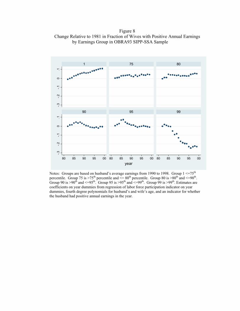
Figure 8 Change Relative to 1981 in Fraction of Wives with Positive Annual Earnings

by Earnings Group in OBRA93 SIPP-SSA Sample

-.3

-.2

-.1

0.1

-.3

-.2

-.1

0.1

80 85 90 95 00 80 85 90 95 00 80 85 90 95 00

1 75 80

90 95 99

year



Figure 9 Mean Change in Earnings Relative to 1981 for Wives in OBRA93 SIPP-SSA Sample by

Earnings Group

Dollar Increase 0

2000

4000

6000

8000

020

0040

0060

0080

00

80 85 90 95 00 80 85 90 95 00 80 85 90 95 00

1 75 80

90 95 99

year


percentile. Group 75 is >75th percentile and <= 80th percentile. Group 80 is >80th and <=90th.Group 90 is >90th and <=95th. Group 95 is >95th and <=99th. Group 99 is >99th. Estimates are coefficients on year dummies from regression of earnings on year dummies, fourth degree polynomials for husband’s and wife’s age, and an indicator for whether the husband had positive annual earnings in the year.

Figure 10 Fraction of Married Women with Positive Annual Earnings by Income Group

in March CPS

0.3

0.4

0.5

0.6

0.7

0.8

1979 1982 1985 1988 1991 1994 1997

P<75

75<=P<80

80<=P<90

90<=P<95

95<=P<99

99<=P

Notes: Groups are based on other household income (husband’s earnings plus asset income) as described in Eissa (1995). Group 1 <=75th percentile. Group 75 is >75th percentile and <= 80th

percentile. Group 80 is >80th and <=90th. Group 90 is >90th and <=95th. Group 95 is >95th and <=99th. Group 99 is >99th.

Comparison of Earnings Distributions from SIPP-SSA Match and Published SSA Tables,

Entire Distribution

Published SSA Tables (top line)

SIPP-SSA Match (bottom line)

CDF

0.0

0.1

0.2

0.3

0.4

0.5

0.6

0.7

0.8

0.9

1.0

1994 Earnings

010000

20000

30000

40000

50000

60000

70000

80000

90000

100000

App

endi

x Fi

gure

1

Appendix Figure 2 Mean Change in Earnings Relative to 1981 for Married Men in

Simulated Cross-Section Version of TRA86 SIPP-SSA Sample by Earnings Group

Dollar Increase 0

1000

0020

0000

3000

000

1000

0020

0000

3000

00

80 85 90 95 00 80 85 90 95 00 80 85 90 95 00

1 75 80

90 95 99

year


100

200

300

4005

0010

020

030

040

0500

80 85 90 95 00 80 85 90 95 00 80 85 90 95 00

1 75 80

90 95 99

year



Appendix Figure 3 Change Relative to 1981 in Fraction of Wives with Positive Annual Earnings

by Earnings Group in Simulated Cross-Section Version of TRA86 SIPP-SSA Sample -.

10

.1.2

-.1

0.1

.2

80 85 90 95 00 80 85 90 95 00 80 85 90 95 00

1 75 80

90 95 99

year



Appendix Figure 4

0

50000

100000

150000

200000

250000

300000

1979 1980 1981 1982 1983 1984 1985 1986 1987 1988 1989 1990 1991 1992 1993 1994 1995 1996 1997 1998

75<=P<80

P<75

80<=P<90

90<=P<95

95<=P<99

99<=P

Calendar Year

1985

dol

lars

CPS Family Income Excluding Wife's Earnings: Groups 1-6

Table 1 Characteristics of Workers with Earnings Above and Below the Social Security Taxable

Maximum Below current

taxablemaximum

Between current taxable maximum and

90% of covered earnings

Above 90% of covered earnings

Mean 1996 Earnings $16,051 $71,869 $172,239 Mean Wages $15,370 $67,296 $146,568 Mean Self Employment $681 $4,573 $25,671

Mean Age 44.7 45.1 46.4 Percent Older than 54 26.2% 15.5% 18.3% Percent Self Employed 7.4% 13.0% 23.8% Percent Married Male 31.3% 68.3% 78.7% Percent Unmarried Male 16.2% 12.6% 8.8% Percent Married Female 33.6% 11.3% 8.9% Percent Unmarried Female 19.0% 7.8% 3.6% Percent White Collar 72.6% 82.6% 93.9% Percent prime age male 30.5% 68.2% 69.7% Percent prime age male not self employed

27.3% 59.2% 52.5%

Note: Data are from the 1996 panel of the SIPP-SSA match as described in the match. Earnings information, including mean wages, mean self employment and percent self-employed come from the administrative earnings records. The other variables come from the SIPP survey.

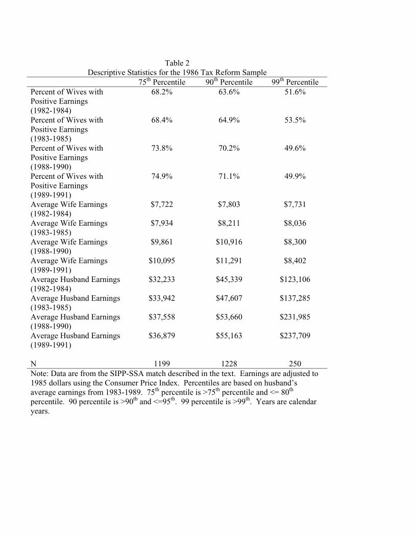
Table 2 Descriptive Statistics for the 1986 Tax Reform Sample

75th Percentile 90th Percentile 99th Percentile Percent of Wives with Positive Earnings (1982-1984)

68.2% 63.6% 51.6%

Percent of Wives with Positive Earnings (1983-1985)

68.4% 64.9% 53.5%


73.8% 70.2% 49.6%


74.9% 71.1% 49.9%

Average Wife Earnings (1982-1984)

$7,722 $7,803 $7,731


$7,934 $8,211 $8,036


$9,861 $10,916 $8,300


$10,095 $11,291 $8,402

Average Husband Earnings (1982-1984)

$32,233 $45,339 $123,106


$33,942 $47,607 $137,285


$37,558 $53,660 $231,985


$36,879 $55,163 $237,709

N 1199 1228 250 Note: Data are from the SIPP-SSA match described in the text. Earnings are adjusted to 1985 dollars using the Consumer Price Index. Percentiles are based on husband’s average earnings from 1983-1989. 75th percentile is >75th percentile and <= 80th

percentile. 90 percentile is >90th and <=95th. 99 percentile is >99th. Years are calendar years.

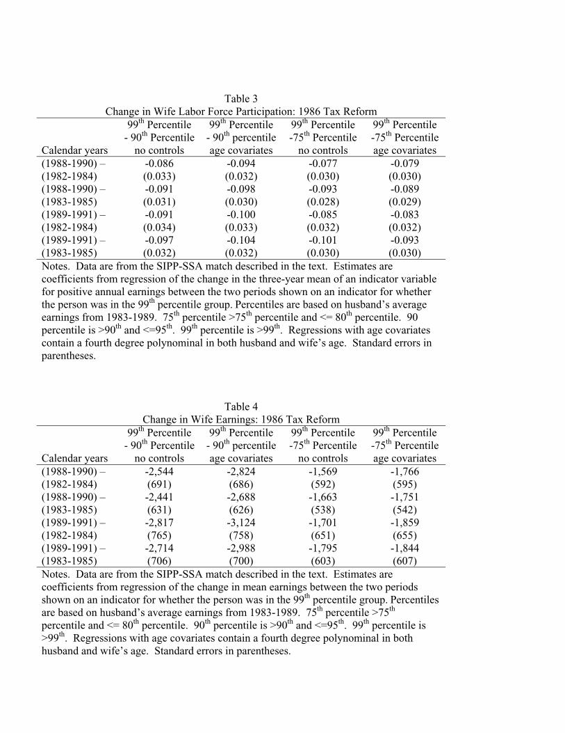
Table 3 Change in Wife Labor Force Participation: 1986 Tax Reform

Calendar years

99th Percentile - 90th Percentile

no controls

99th Percentile - 90th percentile age covariates

99th Percentile -75th Percentile

no controls

99th Percentile -75th Percentile age covariates

(1988-1990) – (1982-1984)

-0.086(0.033)

-0.094(0.032)

-0.077(0.030)

-0.079(0.030)

(1988-1990) – (1983-1985)

-0.091(0.031)

-0.098(0.030)

-0.093(0.028)

-0.089(0.029)

(1989-1991) – (1982-1984)

-0.091(0.034)

-0.100(0.033)

-0.085(0.032)

-0.083(0.032)

(1989-1991) – (1983-1985)

-0.097(0.032)

-0.104(0.032)

-0.101(0.030)

-0.093(0.030)

Notes. Data are from the SIPP-SSA match described in the text. Estimates are coefficients from regression of the change in the three-year mean of an indicator variable for positive annual earnings between the two periods shown on an indicator for whether the person was in the 99th percentile group. Percentiles are based on husband’s average earnings from 1983-1989. 75th percentile >75th percentile and <= 80th percentile. 90 percentile is >90th and <=95th. 99th percentile is >99th. Regressions with age covariates contain a fourth degree polynominal in both husband and wife’s age. Standard errors in parentheses.

Table 4 Change in Wife Earnings: 1986 Tax Reform

Calendar years


no controls



no controls


(1988-1990) – (1982-1984)

-2,544(691)

-2,824(686)

-1,569(592)

-1,766(595)

(1988-1990) – (1983-1985)

-2,441(631)

-2,688(626)

-1,663(538)

-1,751(542)

(1989-1991) – (1982-1984)

-2,817(765)

-3,124(758)

-1,701(651)

-1,859(655)

(1989-1991) – (1983-1985)

-2,714(706)

-2,988(700)

-1,795(603)

-1,844(607)

Notes. Data are from the SIPP-SSA match described in the text. Estimates are coefficients from regression of the change in mean earnings between the two periods shown on an indicator for whether the person was in the 99th percentile group. Percentiles are based on husband’s average earnings from 1983-1989. 75th percentile >75th

percentile and <= 80th percentile. 90th percentile is >90th and <=95th. 99th percentile is >99th. Regressions with age covariates contain a fourth degree polynominal in both husband and wife’s age. Standard errors in parentheses.

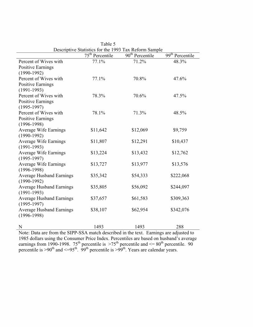
Table 5 Descriptive Statistics for the 1993 Tax Reform Sample

75th Percentile 90th Percentile 99th Percentile Percent of Wives with Positive Earnings (1990-1992)

77.1% 71.2% 48.3%


77.1% 70.8% 47.6%


78.3% 70.6% 47.5%


78.1% 71.3% 48.5%


$11,642 $12,069 $9,759


$11,807 $12,291 $10,437


$13,224 $13,432 $12,762


$13,727 $13,977 $13,576


$35,342 $54,333 $222,068


$35,805 $56,092 $244,097


$37,657 $61,583 $309,363


$38,107 $62,954 $342,076

N 1493 1493 288 Note: Data are from the SIPP-SSA match described in the text. Earnings are adjusted to 1985 dollars using the Consumer Price Index. Percentiles are based on husband’s average earnings from 1990-1998. 75th percentile is >75th percentile and <= 80th percentile. 90 percentile is >90th and <=95th. 99th percentile is >99th. Years are calendar years.

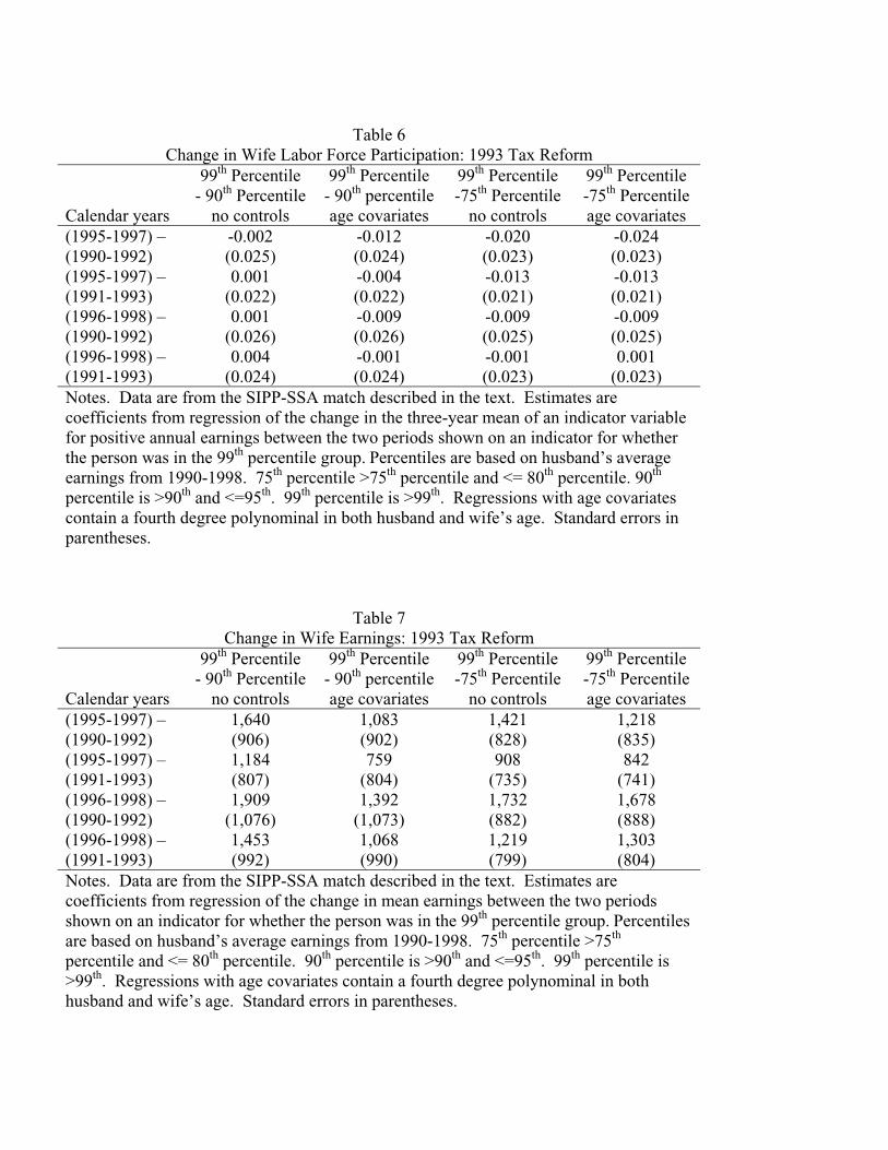
Table 6 Change in Wife Labor Force Participation: 1993 Tax Reform

Calendar years


no controls



no controls


(1995-1997) – (1990-1992)

-0.002(0.025)

-0.012(0.024)

-0.020(0.023)

-0.024(0.023)

(1995-1997) – (1991-1993)

0.001(0.022)

-0.004(0.022)

-0.013(0.021)

-0.013(0.021)

(1996-1998) – (1990-1992)

0.001(0.026)

-0.009(0.026)

-0.009(0.025)

-0.009(0.025)

(1996-1998) – (1991-1993)

0.004(0.024)

-0.001(0.024)

-0.001(0.023)

0.001(0.023)

Notes. Data are from the SIPP-SSA match described in the text. Estimates are coefficients from regression of the change in the three-year mean of an indicator variable for positive annual earnings between the two periods shown on an indicator for whether the person was in the 99th percentile group. Percentiles are based on husband’s average earnings from 1990-1998. 75th percentile >75th percentile and <= 80th percentile. 90th

percentile is >90th and <=95th. 99th percentile is >99th. Regressions with age covariates contain a fourth degree polynominal in both husband and wife’s age. Standard errors in parentheses.

Table 7 Change in Wife Earnings: 1993 Tax Reform

Calendar years


no controls



no controls


(1995-1997) – (1990-1992)

1,640(906)

1,083(902)

1,421(828)

1,218(835)

(1995-1997) – (1991-1993)

1,184(807)

759(804)

908(735)

842(741)

(1996-1998) – (1990-1992)

1,909(1,076)

1,392(1,073)

1,732(882)

1,678(888)

(1996-1998) – (1991-1993)

1,453(992)

1,068(990)

1,219(799)

1,303(804)

Notes. Data are from the SIPP-SSA match described in the text. Estimates are coefficients from regression of the change in mean earnings between the two periods shown on an indicator for whether the person was in the 99th percentile group. Percentiles are based on husband’s average earnings from 1990-1998. 75th percentile >75th

percentile and <= 80th percentile. 90th percentile is >90th and <=95th. 99th percentile is >99th. Regressions with age covariates contain a fourth degree polynominal in both husband and wife’s age. Standard errors in parentheses.

Table 8 CPS Change in Wife Labor Force Participation: 1986 Tax Reform

Calendar years 99th Percentile-90th Percentile

no controls 99th Percentile-75th Percentile

no controls (1988-1990) –(1982-1984)

-0.006(0.028)

-0.000(0.027)

(1988-1990) –(1983-1985)

-0.007(0.028)

-0.008(0.027)

(1989-1991) –(1982-1984)

0.032(0.028)

0.015(0.027)

(1989-1991) –(1983-1985)

0.031(0.028)

0.023(0.026)

Notes. Data are from March Current Population Surveys from years following the indicated calendar years. Estimates are coefficients and standard errors on group99*post reform interaction term in a difference in differences regression.

Table 9 CPS Change in Wife Earnings: 1986 Tax Reform



no controls (1988-1990) –(1982-1984)

-547(828)

93(726)

(1988-1990) –(1983-1985)

-365(853)

466(750)

(1989-1991) –(1982-1984)

756(851)

970(751)

(1989-1991) –(1983-1985)

938(875)

1,342(774)


Table 10 CPS Change in Wife Labor Force Participation: 1993 Tax Reform



no controls (1995-1997) –(1989-1991)

-0.056(0.029)

-0.029(0.027)

(1995-1997) –(1990-1992)

-0.058(0.029)

-0.027(0.027)

(1996-1998) –(1989-1991)

-0.072(0.029)

-0.045(0.027)

(1996-1998) –(1990-1992)

-0.075(0.029)

-0.043(0.027)


Table 11 CPS Change in Wife Earnings: 1993 Tax Reform



no controls (1995-1997) –(1989-1991)

-1,374(1,511)

-347(1,328)

(1995-1997) –(1990-1992)

-1,475(1,550)

-1,004(1,355)

(1996-1998) –(1989-1991)

-1,287(1,601)

-371(1,363)

(1996-1998) –(1990-1992)

-1,388(1,640)

-1,028(1,390)


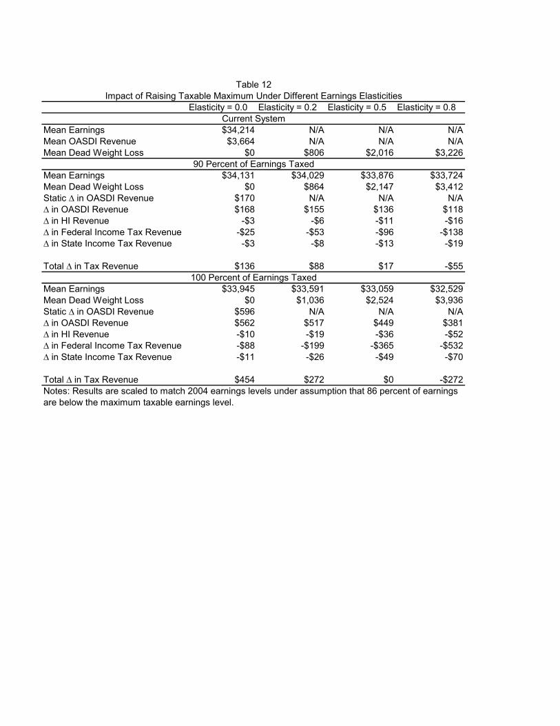
Elasticity = 0.0 Elasticity = 0.2 Elasticity = 0.5 Elasticity = 0.8

Mean Earnings $34,214 N/A N/A N/AMean OASDI Revenue $3,664 N/A N/A N/AMean Dead Weight Loss $0 $806 $2,016 $3,226

Mean Earnings $34,131 $34,029 $33,876 $33,724Mean Dead Weight Loss $0 $864 $2,147 $3,412Static in OASDI Revenue $170 N/A N/A N/A

in OASDI Revenue $168 $155 $136 $118 in HI Revenue -$3 -$6 -$11 -$16 in Federal Income Tax Revenue -$25 -$53 -$96 -$138 in State Income Tax Revenue -$3 -$8 -$13 -$19

Total in Tax Revenue $136 $88 $17 -$55

Mean Earnings $33,945 $33,591 $33,059 $32,529Mean Dead Weight Loss $0 $1,036 $2,524 $3,936Static in OASDI Revenue $596 N/A N/A N/A

in OASDI Revenue $562 $517 $449 $381 in HI Revenue -$10 -$19 -$36 -$52 in Federal Income Tax Revenue -$88 -$199 -$365 -$532 in State Income Tax Revenue -$11 -$26 -$49 -$70

Total in Tax Revenue $454 $272 $0 -$272Notes: Results are scaled to match 2004 earnings levels under assumption that 86 percent of earningsare below the maximum taxable earnings level.

100 Percent of Earnings Taxed

Table 12Impact of Raising Taxable Maximum Under Different Earnings Elasticities

Current System

90 Percent of Earnings Taxed

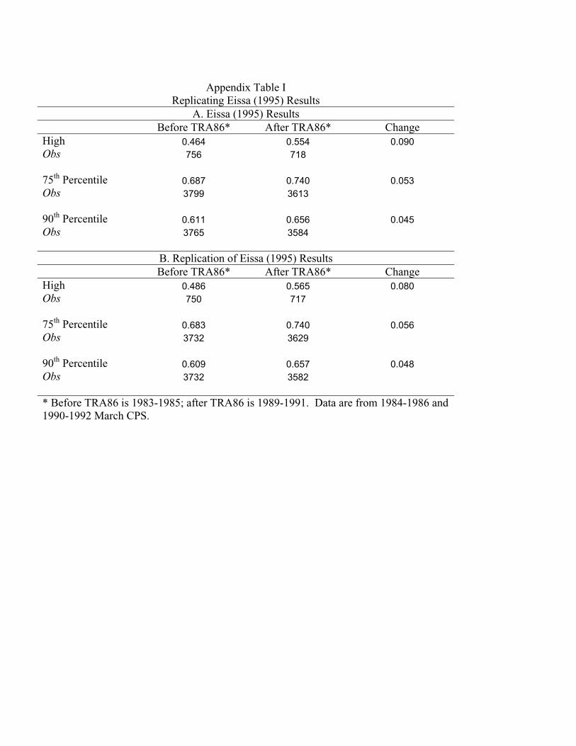
Appendix Table I Replicating Eissa (1995) Results

A. Eissa (1995) Results Before TRA86* After TRA86* Change High 0.464 0.554 0.090 Obs 756 718

75th Percentile 0.687 0.740 0.053 Obs 3799 3613


B. Replication of Eissa (1995) Results Before TRA86* After TRA86* Change High 0.486 0.565 0.080 Obs 750 717



* Before TRA86 is 1983-1985; after TRA86 is 1989-1991. Data are from 1984-1986 and 1990-1992 March CPS.

Appendix Table II Replicating Eissa (1995) Summary Statistics

A. Eissa (1995) Summary Statistics High 75th Percentile 90th Percentile Age 47.6 40.6 42.9 Education 14.8 13.3 14.1 Preschool Children 0.18 0.35 0.31 Family Size 2.88 3.21 3.18 Other Household Income 122,790 37,223 57,386 Hours 696 1092 939

B. Replication of Eissa (1995) Summary Statistics High 75th Percentile 90th Percentile Age 47.7 40.6 42.9 Education 14.8 13.4 14.2 Preschool Children 0.18 0.35 0.32 Family Size 2.77 3.12 3.08 Other Household Income 123,923 37,381 57,876 Hours 738 1092 945 Notes: Data are from 1984-1986 and 1990-1992 March CPS.

Appendix Table III

Details of Eissa Replication SampleCalendar Year 1982 1983 1984 1985 1988 1989 1990 1991

Total CPS obs 162,635 161,167 161,362 157,661 144,687 158,079 158,477 155,796

Observations DroppedAge less than 20 or greater than 64 69,897 68,754 68,475 66,894 61,446 66,777 67,040 65,646

Males 44,704 44,452 44,517 43,676 40,163 43,960 43,980 43,489

Unmarried females* 16,466 16,733 17,243 16,907 15,578 17,601 18,070 17,905

SubtotalMarried females between 20 and 64 years old, inclusive 31,568 31,228 31,127 30,184 27,500 29,741 29,387 28,756

Further Dropped Observations 25,407 25,116 25,175 24,453 21,988 24,302 24,007 23,398Total additional dropped** 6,186 6,127 5,972 5,765 5,535 5,456 5,410 5,380

Wife self-employed*** 1,874 1,869 1,852 1,765 1,998 2,158 2,090 2,004

Wife was disabled**** 674 611 563 542 509 620 588 588

Husband not working***** 3,944 3,973 3,875 3,722 3,306 2,989 2,979 3,055

Wife had excessive hours****** 62 26 39 45 46 44 53 4025 15 20 34 23 17 30 22

Total obs remaining in sample 25,382 25,101 25,155 24,419 21,965 24,285 23,977 23,376*An individual is considered unmarried if she is widowed, divorced, separated, never married, or her spouse is absent.**Total additional dropped does not equal the sum of the subcategories because the subcategories are not mutually exclusive.*** Wife is considered self-employed if she had business or farm self-employment earnings.****An individual is considered disabled if she selected "disabled or sick" for the main reason she did not work last year.*****Husband is not working if husband's weeks worked last year or husband's usual hours worked per week last year equal zero.******Females working greater than or equal to 4,160 annual hours of work.

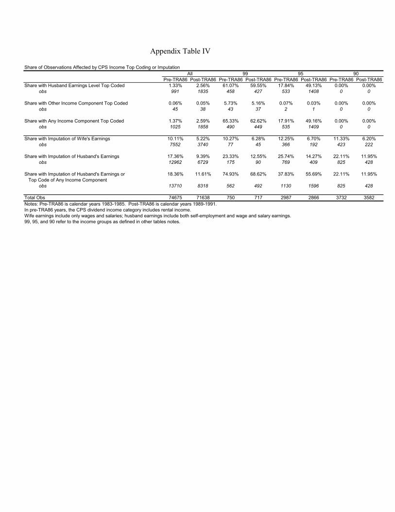
Appendix Table IV

Share of Observations Affected by CPS Income Top Coding or Imputation

Pre-TRA86 Post-TRA86 Pre-TRA86 Post-TRA86 Pre-TRA86 Post-TRA86 Pre-TRA86 Post-TRA86Share with Husband Earnings Level Top Coded 1.33% 2.56% 61.07% 59.55% 17.84% 49.13% 0.00% 0.00%

obs 991 1835 458 427 533 1408 0 0

Share with Other Income Component Top Coded 0.06% 0.05% 5.73% 5.16% 0.07% 0.03% 0.00% 0.00%obs 45 38 43 37 2 1 0 0

Share with Any Income Component Top Coded 1.37% 2.59% 65.33% 62.62% 17.91% 49.16% 0.00% 0.00%obs 1025 1858 490 449 535 1409 0 0

Share with Imputation of Wife's Earnings 10.11% 5.22% 10.27% 6.28% 12.25% 6.70% 11.33% 6.20%obs 7552 3740 77 45 366 192 423 222

Share with Imputation of Husband's Earnings 17.36% 9.39% 23.33% 12.55% 25.74% 14.27% 22.11% 11.95%obs 12962 6729 175 90 769 409 825 428

Share with Imputation of Husband's Earnings or 18.36% 11.61% 74.93% 68.62% 37.83% 55.69% 22.11% 11.95%Top Code of Any Income Component

obs 13710 8318 562 492 1130 1596 825 428

Total Obs 74675 71638 750 717 2987 2866 3732 3582Notes: Pre-TRA86 is calendar years 1983-1985. Post-TRA86 is calendar years 1989-1991.In pre-TRA86 years, the CPS dividend income category includes rental income. Wife earnings include only wages and salaries; husband earnings include both self-employment and wage and salary earnings.99, 95, and 90 refer to the income groups as defined in other tables notes.

All 99 95 90

earnings responses to increases in payroll taxessaez/liebman-saezssa06.pdf · earnings responses to...

Documents