1

Confidence W. Amadi cwamadi@mail.ecsu.edu is an Associate Professor of Finance, Department of Accounting, Finance, and Economics, Walter R. Davis School of Business and Economics, Elizabeth City State University.

Abstract

The estimation of the cost of equity has been the most daunting of all the variables essential for asset valuation. The most widely used methods for its determination are the Gordon model, the capital asset pricing model (CAPM), the cost of debt plus a risk premium, the arbitrage pricing theory (APT) and the residual income model (RIV). The Gordon model is limited to firms that pay dividends that are assumed to grow at a constant rate. The CAPM is based on a diversified portfolio, and the long-run concept in which the required, expected and realized returns are the same. The cost of debt plus risk premium assumes a levered firm, but does not specify how the risk premium should be determined. The APT is an extension of the CAPM with multiple, albeit, unspecified risk factors. The RIV model solves for the discount rate that equates the present value of the “excess income” to the current stock price. The objective of this paper is to introduce a model for the cost of equity that is based on the relationship between the earnings, the opportunity cost of funds and the concept of risk as the chance of a loss.

2

Introduction The Gordon model is limited to firms that pay dividends that are assumed to grow at a constant rate. It implicitly assumes that the current stock price is the intrinsic value of the firm. Explicitly, the Gordon model calculates the return that equates the present value of the expected dividend stream to the current stock price. The CAPM is based on a diversified portfolio, and the long-run concept in which the required return, expected return and realized return converge to the same value, a concept that only holds in a static environment. In the accounting profession, a variance of the Gordon model, the residual income model (RIV) provides a means for calculating the cost of equity based on a terminal value of the stock price, the earnings of the firm and the current stock price. Aside from the obvious difficulty in estimating the terminal value of the firm‟s stock price, the derived cost of equity relies on the current stock price. By definition, the current stock price is what the last purchaser of the stock paid for the last share of stock bought. Investors sell or buy stock based on the relationship between the current price and the investors‟ perceived intrinsic value of the stock. In general, trades occur when either the participants believe at the minimum that the security is fairly priced or they have opposing views of over-valued (the seller) and under-valued (the buyer). For listed securities, there exists a wide range of prices based on various investors‟ perception of the value of the security. The current market price is merely the view of the last purchaser. Like all assets, the demand curve of securities must be downward sloping. Conversely, the supply curve is upward sloping. Unlike other assets, where the intersection of the demand and supply curve represents the equilibrium quantity and price, for securities, the market price is the maximum price consumers are willing to pay to buy a unit of the security at the point in time. As a result, using the current stock price in the determination of the cost of equity raises the question of “whose cost of equity”? The cost of debt plus a risk premium is another model that is gaining some attention (Lasher, 2002). Under this model, the cost of equity is the firm‟s cost of debt plus a risk premium. “The increment in risk between debt and equity is about the same for high-risk and low-risk firms. That increment tends to command an additional premium of between 3 percent and 5 percent” (p.398). The use of the model is limited to firms that have debt in their capital structure. Moreover, since firms issue debt with various maturities and covenants, the choice of the appropriate cost of debt becomes a concern.

3

There is a universal agreement that the higher the risk, the higher the required

return. Unfortunately, there is no single accepted definition of risk. Alles (1995) presents an overview of the various investment risk concepts and how they are measured. Although standard deviation of returns is often viewed as a measure of risk, the introduction of portfolio diversification and its attendant systematic risk has brought into question its validity. Megginson (1997) defines risk as “the chance of a financial loss”. He goes on to say that “the term risk is used interchangeably with uncertainty to refer to variability of returns associated with a given asset” (p95). Thus, in both the capital asset pricing model and the arbitrage pricing theory, it is the later definition of risk as variability from expected return that has prevailed. This concept of risk has very serious limitation.

Consider an investment whose return on investment (ROI) has the following

equally likely outcome: 12 percent, 15 percent, 20 percent, 25 percent, 35 percent and 40 percent. This investment return has variability, but is it risky? The risk-free rate is the required return for deferring consumption. It is purely the time value component of return. In the example above, if the risk-free rate were 7%, it can be seen that the investment has no risk. This is because the worst possible outcome is 5% higher than the risk-free rate. This investment has all possible returns that are higher than the required return based purely on time preference for consumption. As a result, its cash flow should be discounted using the risk-free rate of return. This is the basis for this paper.

The objective of this paper is to present a model of asset pricing that is based on

the chance of a loss definition of risk. The rest of the paper is organized as follows: Section 2 gives a brief literature review of the role of earnings in security pricing; Section 3 presents a brief overview of the most common asset pricing models, and Section 4 presents the chance of a loss (COL) model of risk measurement and asset pricing, Section 5 is on data and methodology, Section 6 presents the results and Section 7, analysis and conclusion.

Brief Role of Earnings Literature Review

The purpose of this review is to focus or draw attention to the role of earnings in

security valuation. Its role in valuation of assets, via dividend payout and retention ratio, is a well established in finance textbooks and academic literature.

4

Botosan and Plumlee (2005), explore the relationship between five measures of

the cost of equity and firm risk with the objective of determining the most appropriate method for calculating the firm specific cost of equity. In their study, the arbitrage pricing theory (APT) is used to calculate the risk premium. The risk factors were identified as unlevered beta from the capital asset pricing model, leverage, “information risk”, market value of equity, book-to-price ratio, and earnings growth. The five methods used for deducing the cost of equity only differed by the method of estimating the terminal value of the firm‟s stock price. Thus, the estimated cost of equity was only as valid as the forecast of the terminal values. Even then, only two of the models were “consistently and predictably related” to their definition of risk.

Francis et al (2004) examined the relationship between the cost of equity capital

and seven attributes of earnings and concluded that accounting based attributes such as accrual earnings, has the largest impact on the cost of equity. Their results indicate that the cost of equity is related to earnings, even though the cost of equity under investigation is the Value-Line estimate of the cost of equity. Since Value-line does not disclose the methodology used in its estimate of the cost of equity, the explanatory power could possibly be due to multi-co linearity, if some of the same earnings attributes were used in the estimation.

Daske et al (2006), using the residual income valuation model, estimates a firm‟s

expected cost of equity “derived from its stock price and analysts‟ consensus earnings forecasts”. The strength of the model is supposed to lie in the use of expected earnings. This is an ordinary conditional forecasting in which, according to Pindyck and Rubinfeld (1991) “the stochastic nature of the predicted value of the X‟s will lead to forecasts of Y which are less reliable than in the fixed-X case” (p195). In this case, the analyst‟s stock price estimate is the X-variable, while the cost of equity is the Y-variable. Consequently, the estimated cost of equity is the implied cost of equity that is consistent with the analysts‟ forecast and its reliability is subject to the analyst‟s forecast. The authors in this case use the median of the analyst forecast.

Cheng (2005) investigated the determinants of residual income by analyzing the

impact of value-creation and value-recording processes on abnormal return on equity. They show that the abnormal return on equity (ROE) is positively related to accounting factors, industry monopoly power, and firm monopoly power.

Gode and Ohlson (2004) introduced stochastic interest rates into the “mark-to-market” and “income-statement approach” to valuation. In the mark to market model, book value equals market value. The income-statement approach assumes that

5

earnings have sufficient information for valuation.They show that the residual income decreases with increase in the beginning period risk-free rate. They demonstrate that the information content of current accounting data decrease with increase in the level of interest rates.

Borgman and Strong (2006) by combining the cost of equity function of the

capital asset pricing model and the constant growth model, and relaxing the zero growth inherent in the development of the weighted average cost of capital, show that increase in the earnings growth rate reduces the systematic risk of the firm and hence the required return on equity. Wei and Zhang (2006) using the data from 1976 to 2000 in the US stock markets show that “stock return volatility is negatively related to the return on equity and positively related to the volatility of the return on equity in cross-sections. Nissim and Penman (2003) show that changes in interest rates have a dual effect on stock price. They show that changes in interest rates are negatively related to residual earnings by affecting the rate at which earnings are charged to the book value of equity used in generating the earnings. Changes in interest rate also affect the level of operating income.

In finance textbooks such as Ross et al (2006), students are taught that cash

flow is supreme in the valuation and other operating decisions of the firm. While this may be true for capital budgeting purposes, Francis et al (2003) show that across the board, earnings dominate other performance measures (even in industries where other measures are preferred) in explaining “ex ante security returns”.

The preceding review highlights the significance of earnings in security valuation.

Most of the studies use earnings or its derivative as the numerator of the valuation equation. Although studies have documented the response of security prices to earnings announcement surprises (see Miller 2005), the role of determining the risk of firms has been confined to risk factors such as size, beta, book-to-market ratio, etc. Earnings variability has not figured prominently in this endeavor.

Factors Affecting the P/E (E/P) Ratio

The price-earnings (P/E) ratio is commonly used as a measure of the growth potential and the riskiness of the firm‟s cash flow. The higher the P/E ratio, the higher the expected growth rate in earnings and or the lower the perceived riskiness of the firm‟s cash flow. Low P/E ratio stocks have been termed “value stocks”. Low P/E ratio could also be used to identify “fallen angels”. Low P/E ratio stocks characterize firms with poor growth potential and /or high risk cash flows. The chance of a loss model

6

(COL) relies on this attribute of the P/E ratio and is based on its reciprocal, the earnings yield (E/P).

Constand, Freitas and Sullivan (1991), examined the factors that affect the E/P

ratios and market value of Japanese firms. They documented a positive relationship between changes in the standard deviation of earnings (as a proxy for risk), expected earnings growth rate and change in dividends per share. Amoako-Adu and Smith (2002) analyzed the causal relationship between the yield on the 3-month Treasury bill and the average P/E ratio of the Toronto Stock Exchange (TSE) and seven major Canadian industry indices. They found a very strong inverse relationship between the treasury yield and the average P/E ratio, with an adjusted R-squared of 95% for the TSE 300 Index. The utilities industry had the highest R-squared (98%), while the gold and silver industry had the lowest (84 percent).

By calculating the P/E ratio using earnings averaged over a period of eight years, Anderson and Brooks (2006) were able to significantly increase the return premium of value stocks over glamour stocks. Beneda (2002) show that for periods in excess of 14 years, high P/E portfolios out performed lower P/E ratio portfolios, but with an investment horizon of five years, the growth stocks (high P/E) lagged behind value (low P/E) stocks. Bhargava and Malhotra (2006), studied the effect of price-earnings ratio on world and US indices. They conclude that (after adjusting for statistical estimation problems) price-earnings ratios did not have a significant impact on either future stock prices or earnings yield. Anderson and Brooks (2005) showed that the P/E ratio of a company was influenced by market-wide P/E ratio, the industry sector and the firm size. They showed that after adjusting for the effect of these variables, the ability of the P/E ratio to explain differences in future returns between “glamour stocks and value stocks” was doubled. The literature on the P/E ratio has focused almost exclusively on the explanatory or predictive power of the P/E ratio with respect to returns on equity security. The P/E ratio has been looked upon as the independent variable; this is in contrast to the Federal Reserve – Type model. The Federal Reserve model is an empirical model that captures the the inverse relationship between P/E multiples and interest rates” (Malkiel, 2004). This inverse relationship can be linked to the increase or decrease in the opportunity cost of funds as proxied by the yield on the Treasury security. The higher the opportunity cost of funds, the lower the present value of expected cash flows from an investment. Stock price, as the present value of expected dividends declines with

7

increase in opportunity cost. For a given earnings, this results in a decline in the P/E multiple.

Malkiel reported the explanatory power of the ten-year Treasury yield on the variability of the P/E (E/P) ratios for the period from 1970 through 2003. The study also reported the effect of adding a cost variable in enhancing the explanatory power of the model to a 78% adjusted R-squared. Malkiel listed three main criticisms of the limitations of the Fed-type model as follows: (1) It regresses a nominal variable (return on the ten-year Treasury) against a real variable, P/E multiple; (2) It describes the determination of the market P/E multiple without reference to future market returns: and (3) It takes a back seat to the “Campbell-Shiller” model that predicts future returns. The dependence of the P/E (E/P) ratio on the 10-year treasury yield suggests another role of the ratio. It suggests that the P/E ratio maybe a proxy for the required and/or realized return relative to the risk-free rate. The objective of this paper is to bring to light this new role, and to show how this role accounts for the explanatory power of the various models that rely on the E/P (P/E) ratio as the independent variable.

According to Rutterford (2004), “the first equity valuation techniques used were dividend yield and book value, reflecting early equity investors‟ perception of shares as quasi-bonds, differing only from bonds in the uncertainty of their maturity and of their dividend payments.”

The P/E (E/P) ratio is arguably the most commonly used valuation method. This stems from the early roots of valuation in which both dividends and firm growth are deeply rooted in the effect of the firm‟s earnings on retained earnings. The earnings yield, if based on the current price and the following 12-month earnings, is the return the investor would have earned if the firm followed a 100 percent dividend payout. This is analogous to the current yield of bonds. The model advocated in this paper is a marriage of the Campbell-Shiller and the Federal Reserve-type models. The Campbell-Shiller model is a modified constant growth (Gordon) model. It replaces the stock price in the Gordon model with P/E ratio by dividing both sides of the equation by the earnings (E). The 10-year yield on the treasury is a proxy for the opportunity cost of funds tied up in the stock, hence the direct relationship between the earnings yield and interest rate. As shown by Campbell & Shiller (1998) future growth rates are not related to initial dividend yields or earnings multiple. The inverse relationship of the Campbell-Shiller model could be that the P/E ratio serves as a proxy for the riskiness of the underlying security.

8

This paper explores the role of earnings yield in the determination of the risk of

equity securities. Miller and Leiblein (1996) from an extensive review of the literature on down-side risk, documents that although managers and strategic theorists focus on the relevance of downside risk, empirical strategy and organizational research continue to employ operational measures of risk reflecting variability in accounting or stock returns.

The discrepancy between these two measures of risk biases the validity of variance risk measures and the findings based on its concept. Miller and Leiblein go on to show that proxies for downside risk have more explanatory power in relations with return than did risk measures based on the standard deviation of the returns. Malkiel (2004) using the returns on the 10-year Treasury bill as the normal return or the opportunity cost of holding equity securities, demonstrated that the Federal Reserve-type models are far more effective in predicting both future returns and excess returns than is the simple Campbell-Shiller mean reversion model.

Dunis and Reilly (2004) evaluated the performance of portfolios of UK stocks constructed on a value-growth axis using relative valuation measures of price-earnings ratio, dividend yield, price-cash flow ratio, price-book ratio, and market capitalization. They found that the „value‟ portfolio outperformed the „growth‟ portfolio both in nominal terms and after adjusting for risk using the Sharpe ratio. Although their finding is significant, it fails to address the determinants of the value of these relative valuation measures and their relationship to the concept of value and growth. Fisher and Statman (2006) looked at P/E ratio and dividend yield as sentiment indicators on the assumption that stock prices reflect both sentiment and value.They found that even though both direct measures of sentiment index (as reflected by the ratio of bearish to the sum of bearish and bullish financial market newsletters, and P/E) have use as market-timing tools, they have very low reliability. Low P/E ratios relative to the mean reflect a bearish sentiment, and vice versa.

The preceding review highlighted the critical role of P/E ratio in security valuation. This role is explored in greater depth and is found to be a significant variable in quantifying the risk of an asset and hence its required return.

Overview of Asset Pricing Models

The capital asset pricing model (CAPM) has for the past several decades been

the dominant method for estimating the cost of capital that explicitly quantifies the risk of an asset.

9

The CAPM expresses the cost of equity as: Ri = Rf + βi(Rm –Rf) (1) Where: Ri and Rm are the expected required return on security i and the market portfolio, respectively. Rf is the risk free rate of return and βi is the covariance of the returns on security i relative to the market portfolio. Unfortunately, the model has performed poorly (Fama and French, 1992) in explaining the cross-sectional returns. Rolls (1977) criticized the model on several grounds, notably the expectational aspect of the model as well as the use of a proxy for the market portfolio of ALL risky assets. Most of the work on asset pricing has focused on overcoming these limitations.

The problem is that the model is not a realistic model. Its assumptions are at best very limiting. Most important of all, the model relies on security/asset returns and neglects the earnings of the security, a key variable in the determination of returns. The higher the firm‟s income relative to the expected average earnings of the market portfolio, the higher the return on the security relative to the return on the market. This translates into a higher measure of risk. Security returns have two components, the income component and price appreciation. Price appreciation depends on the effect of new information on the magnitude, timing and risk of the expected cash flow from the asset. With the CAPM, the variability in returns relative to the market portfolio determines the risk of an asset. It does not directly consider the most important component of an asset‟s risk: the variability in the asset‟s cash flow.

The CAPM relies on the redefinition of risk as “variability from expected return”.

Yet, the model ignores the factors that affect the expected return. The relevant expected return is, in practice, the historical average return of the security or portfolio. The usefulness of this average depends on the assumption that the future will be like the past (adaptive expectation). However, the environment as well as the market, is dynamic. The ability of the CAPM to explain security or portfolio returns depends on a model that relies on the variability of realized returns relative to that of a market portfolio.

For more than three decades, numerous studies on the CAPM have been

published addressing and modifying the original CAPM. Most recently, Bali et al (2009) examined the cross-sectional relationship between conditional betas and expected stock returns for a sample period from July 1963 to December 2004. They find that it explained between 2.02 percent and 2.13 percent of the cross-sectional variation in

10

returns. Addition of size and book-to-market ration increased the R2 values to between 4.7 percent and 4.87 percent. The question is: “what about the 95+ percent of the variation in the returns”? The fact that a model that only explains such a small fraction of the dependent variable is the standard for the finance profession is truly disturbing.

The arbitrage pricing theory (APT) of Ross (1976) was proposed to enhance the

explanatory power of the CAPM. It contends that security returns are affected by other risk factors. The APT suffers from the same limitation as the CAPM. The risk factors are unknown, and like the CAPM, it relies on asset returns to determine the priced risk factors.

Another common method for estimating the cost of equity is the constant growth

dividend model. This model relies on the firm paying a dividend that is growing at a constant rate indefinitely. It also requires that the price of the stock is known, a priori. This defeats the objective of using the required return to determine the stock price. The constant growth dividend model determines the internal rate of return that equates the expected dividends to the current price of the stock. Moreover, it does not address the risk of the investment.

The residual income valuation model (RIV) is supposed to address the case of

non-dividend paying firms by relying on the earnings of the firm. As depicted in Cheng (2005) the RIV model is described by the following equation: (2)

Where: BVt is the book value of equity, Et(.) is the expectation at time t, Xt is the net income, and r is the cost of equity.

It views the stock price as the sum of the firm‟s book value of equity plus the present value of the residual income.Thus, the cost of equity is the discount rate that both determine the magnitude of the residual income as well as its present value. The RIV estimate depends on the terminal value of the earnings. The higher the terminal value of the earnings, the higher the required return and by inference, the higher the

1

1 1

t tt t t

X rBVV BV E

r

11

riskiness of the asset. Accuracy in the forecast of future earnings and therefore,

terminal value, limits the reliability of the estimated required return. Moreover, the book value of equity is a netted account over the life of the firm. The equity account depends on the

firm‟s earnings as well as the dividend policy. In addition, RIV model does not explicitly address the risk of the earnings.

The cost of debt plus a risk premium is the simplest of these models. It posits

that the cost of equity be equal to the cost of debt plus a risk premium. The required cost of debt is usually the cost the firm‟s long-term debenture. For firms with no long-term debt, this is a problem. Moreover, the determinants of the risk premium are unspecified. It is left to the user to determine the appropriate premium to use. The models discussed above have very serious limitations. The chance of a loss model is proposed as a solution to the problems inherent in these models.

Chance of a Loss (COL) Model

The chance of a loss (COL) model relies on the notion that economic units want

compensation for taking risk, with risk defined as the “chance of a loss”. The higher the chance of a loss, the riskier is the investment perceived and therefore the higher the required return necessary to entice economic units to bear that risk. The required return on any investment has two components: the risk free rate and the risk premium. The risk premium in the model proposed in this paper is strictly based on the chance of loss concept. The risk free rate is the compensation for the time value of money. It is the rate of transformation of present consumption into the future. Thus, when the chance of a loss is zero, the required return for discounting the expected cash flow will be the risk free rate. In the limit, when the chance of a loss tends to one, the required return tends to infinity, meaning that the project will have zero value. With the above restriction, the chance of a loss model is developed as follows:

Let: Rf represent the risk-free rate of return μ represent the probability that the return will be greater than Rf.

represent a measure of the marginal investor‟s risk aversion. The higher the value of in absolute terms, the higher the required return.

represent a constant multiplier Rq represent the required return

12

Then the chance of a loss model is represented by the following function:

(3)

This functional relationship meets the required condition that if the chance of earning less than the risk free rate is zero, the required return should equal the risk free

rate. This condition requires that must equal one. If is less than one, a risk-free asset will be valued less than the yield on the US treasury, which is assumed to be the

risk-free rate. On the other hand, if is greater than one, a risk-free asset will be higher than the accepted risk-free rate. Also the above function meets the condition that if the chance of earning less than the risk free rate is one, the project will require an infinite return and thus, must be rejected.

The chance of a loss for equity investment is determined by the distribution of the

earnings yield (E/P). The equity holders have a residual claim on the earnings of the firm. This is the net income. The E/P represents what the firm earned for its owners per dollar of the net amount invested in the firm for the year as measured by the beginning of the year‟s stock price. The earnings (E) represent the sum of the dividend (which the shareholders receive) and the retained earnings which through the board of directors, they have elected to reinvest in the business. The stock price (P) is the firm‟s stock price at the beginning of the fiscal year.

This study makes the simplifying assumption that all firms have a calendar fiscal

year. The follows the practice of computing P-E ratios and dividend yields based on trailing twelve-month periods even though earnings and dividends are on a quarterly basis. This assumption allows the use of the same treasury yield for all the firms rather than identifying the auction yield corresponding to the firm‟s fiscal year. This earnings yield is the return that is available to investors for comparison against their opportunity cost (assumed the yield on the Treasury security). The probability of this yield being less than the risk-free rate is proposed as a valid measure of the riskiness of the investment.

13

The use of earnings in this model may raise concern since it includes both

dividend and retained earnings. The finance profession tends to focus on free cash flow available to suppliers of capital. The main cash flow available to equity holders is closely approximated by the sum of net income and depreciation. In order for the firm to continue as a going concern, it must continually replenish its productive capacity. Depreciation is the firm‟s best estimate of the reduction over the fiscal period of that productive capacity. Consequently, it is the minimum investment needed to maintain the firm‟s productive capacity. Thus, the net income is an approximation of the maximum cash flow available to share holders that is consistent with maintaining the firm‟s productive capacity.

The COL model over comes one of the major limitations of the CAPM in that it is easily tested. It can be argued that investors look at the historical performance of the firm in trying to form an opinion about its future prospects. Given this condition, the historical distribution of the firm‟s E/P and the return on the Treasury security of identical maturity as the investment horizon, will provide an estimate of the probability k of E/P being less than the risk-free rate. μ can then be estimated as (1-k). Pindyck and Rubinfeld (1991, p24), show that the mean of a sample is the unbiased estimator of the true population mean. Thus, we can use the mean of the risk-free rate and the cross-sectional distribution of average return over the investment horizon and the μ values for

each firm to estimate the coefficients and using the following equation:

= ln + lnRf - ln μ + (4) Where:

is the natural log of the average return

is the coefficient

is an error term. Equation (4) is the empirical version of equation (3). To show how the model can be

used to estimate the cost of equity, let the risk-free rate be 5 percent, and be equal to

1, then for various values of μ and the required return Rq can be calculated. The result of such exercise is presented in Table 1 and its plot in Figure 1. Both are shown below.

14

TABLE 1

REQUIRED RATE OF RETURN FOR VARIOUS μ AND

Risk-free rate = 0.05 = 1

Gamma 0.1 0.2 0.5 0.6 0.75 1 1.2 1.5 1.8 2 2.25 2.5 2.75 3

Probability μ (%)

REQUIRED RETURN (%)

2.00 7.39 10.93 35.36 52.28 94.02 250.0 546.6 1767. 5716. 12500. 33239. 88388.35%

235037.69%

625000.00%

5.00 6.75 9.10 22.36 30.17 47.29 100.0 182.0 447.2 1098. 2000.0 4229.4 8944.27% 18914.83% 40000.00%

7.50 6.48 8.39 18.26 23.66 34.89 66.67 111.9 243.4 529.4 888.89 1698.5 3245.76% 6202.28% 11851.85%

10.00 6.29 7.92 15.81 19.91 28.12 50.00 79.24 158.1 315.4 500.00 889.14 1581.14% 2811.71% 5000.00%

15.00 6.04 7.31 12.91 15.61 20.74 33.33 48.71 86.07 152.0 222.22 357.08 573.78% 921.97% 1481.48%

25.00 5.74 6.60 10.00 11.49 14.14 20.00 26.39 40.00 60.63 80.00 113.14 160.00% 226.27% 320.00%

30.00 5.64 6.36 9.13 10.30 12.33 16.67 21.20 30.43 43.67 55.56 75.07 101.43% 137.05% 185.19%

35.00 5.55 6.17 8.45 9.39 10.99 14.29 17.62 24.15 33.09 40.82 53.07 68.99% 89.70% 116.62%

40.00 5.48 6.01 7.91 8.66 9.94 12.50 15.01 19.76 26.02 31.25 39.29 49.41% 62.13% 78.13%

42.50 5.45 5.93 7.67 8.35 9.50 11.76 13.96 18.05 23.33 27.68 34.28 42.46% 52.59% 65.13%

45.00 5.42 5.87 7.45 8.07 9.10 11.11 13.04 16.56 21.05 24.69 30.15 36.81% 44.94% 54.87%

47.50 5.39 5.80 7.25 7.82 8.74 10.53 12.22 15.27 19.10 22.16 26.69 32.15% 38.73% 46.65%

50.00 5.36 5.74 7.07 7.58 8.41 10.00 11.49 14.14 17.41 20.00 23.78 28.28% 33.64% 40.00%

55.00 5.31 5.64 6.74 7.16 7.83 9.09 10.25 12.26 14.67 16.53 19.19 22.29% 25.88% 30.05%

60.00 5.26 5.54 6.45 6.79 7.33 8.33 9.23 10.76 12.54 13.89 15.78 17.93% 20.37% 23.15%

65.00 5.22 5.45 6.20 6.47 6.91 7.69 8.38 9.54 10.86 11.83 13.18 14.68% 16.35% 18.21%

70.00 5.18 5.37 5.98 6.19 6.53 7.14 7.67 8.54 9.50 10.20 11.16 12.20% 13.33% 14.58%

75.00 5.15 5.30 5.77 5.94 6.20 6.67 7.06 7.70 8.39 8.89 9.55 10.26% 11.03% 11.85%

80.00 5.11 5.23 5.59 5.72 5.91 6.25 6.54 6.99 7.47 7.81 8.26 8.73% 9.24% 9.77%

85.00 5.08 5.17 5.42 5.51 5.65 5.88 6.08 6.38 6.70 6.92 7.21 7.51% 7.82% 8.14%

90.00 5.05 5.11 5.27 5.33 5.41 5.56 5.67 5.86 6.04 6.17 6.34 6.51% 6.68% 6.86%

95.00 5.03 5.05 5.13 5.16 5.20 5.26 5.32 5.40 5.48 5.54 5.61 5.68% 5.76% 5.83%

98.00 5.01 5.02 5.05 5.06 5.08 5.10 5.12 5.15 5.19 5.21 5.23 5.26% 5.29% 5.31%

100.0 5.00 5.00 5.00 5.00 5.00 5.00 5.00 5.00 5.00 5.00 5.00 5.00% 5.00% 5.00%

15

Figure 1

For the marginal investor or the market, the risk tolerance factor and the

coefficients and can be empirically determined from cross-sectional data on returns. Since the required return is not observable, equation (3) must be recast in a form that uses readily available information, such as the observed return on a stock. The period realized return is readily available and adequately fulfills that role. Using this realized period return, and normalizing equation (3) by dividing both sides with the period realized risk free rate, equation (4) can be represented as: Ω = δ - γln μ + ε (5) Where:

1.00%

10.00%

100.00%

1000.00%

10000.00%

100000.00%

1000000.00%

0.00% 20.00% 40.00% 60.00% 80.00% 100.00% 120.00%Req

uir

ed

Retu

rn (

log

scale

)

Probability

0.1

0.2

0.5

0.6

0.75

1

1.2

1.5

1.8

2

2.25

2.5

2.75

3

16

Ω is the natural log of the ratio of the period return on the security to the return on the risk-free security. Taking the natural logarithm of the normalized equation 3, linearizes the model such the linear estimation of the parameters are possible. δ is a constant and γ and ε are as in equation (4).

In an efficient market, the required return on a risk-free asset must equal the risk-

free rate. Thus, δ (which is ln , and with = 1.0) will be zero. This model assumes that the market is long-run efficient in terms of the weak and semi-strong efficient market theories.

Data and Methodology

The sample firms studied are the 65 firms in the Dow Jones Composite index and consisted of firms with at least 20 years of annual data. This restriction resulted in 50 useable firms; the sample size increased to 54 when the estimation period length was reduced. The sample period is from 1985 through 2007. The earnings yield was based on the beginning of the year stock price and the earnings per share for that year. The realized earnings yield is what the investor could have earned on their investment if the firm had a 100 percent dividend pay-out ratio.

The annualized return on the 3-year, 5-year, and 10-year US Treasury notes were used as the risk free opportunity cost to the investor. The values are the beginning of the year auction yields.The yields on these US securities over the sample period were contrasted with the return for each firm to determine the probability of earning more than the risk-free rate. The probability of earning yield being more than the risk-free rate is determined for the sample firms for each of the reference Treasury securities. Two sets of probability distributions were determined based on twenty and ten years of historical data. For each Treasury security, the corresponding realized return for the firm is normalized using the average realized return on the US Treasury security. Equation 5 was estimated using 3-, 5-, and 10-year realized cross-sectional returns of the sample firms. The statistical package used is the basic Microsoft Excel. This package is readily available to investors and hence the average investor without difficulty can adopt the results.

Results

In this section the results of ordinary least squares regression analysis of the

chance of a loss model is presented. The results of the OLS regression of the normalized average annual returns and the probability of earning more than the yield on

17

the Treasury security is presented in Table 2 below. The residual plots for each of the models indicate that it is safe to assume that the error terms are homoskedastic. The OLS results indicate that the probability of earning more than the yield on the risk-free security is highly significant in explaining the average return on the sample firms. Except for the 10-year return/10-year estimation period, the sign of the exponent of the probability variable (γ) is negative and consistent with the premise of the chance-of-a-loss model.

Table 2 Results of the OLS Estimation of Probability of Earning More than the Risk-free Rate Against the Normalized Average Return

PEP10 PEP20 AR3 AR5 AR10 AR3 AR5 AR10 Gamma -0.4533 -0.7513 0.1554 -0.2254 -0.4125 -0.0055 t-statistic -2.644 -4.9255 1.3341 -2.0453 -4.1939 -0.0853 P-value 0.0109 8.63E-06 0.1883 0.0461 0.0001 0.9324 R-squared 0.1227 0.314 0.3505 0.0772 0.2492 0.00015 F-statistic 6.991 24.26 1.7797 4.1831 17.5887 0.0073 F-significance

0.011 8.93E-06 0.1885 0.0462 0.00011 0.9324

SER 1.3325 1.2911 0.9443 1.3666 1.3507 0.9612 N 51 54 50 51 54 50 AR(i) is the natural log of the ratio of the firms average return over holding period (i), in years, of the firm and the average return on the (i)-year Treasury security over the (i) holding period. PEP(j) is the estimation period (years) for the probabilities. The independent variable is Ln μ (j)t(i) is the natural log of the probability of earning more than the risk-free rate over period (i), estimated over period (j), where (i) and (j) are the holding period and estimation periods, respectively. Gamma is the estimate of the exponent of the probability variable.

The results indicate a strong dependence of γ on both the holding period and the estimation period. In all the variations of the OLS, the absolute value of γ decreased with increase in the estimation period. Gamma (γ) as a measure of the average level of risk averseness is positively related to the holding period. For the 10-year estimation period, an increase from 3 to 5 year holding period resulted in a change in γ from -0.4533 to -0.7513, denoting a 65.7 percent increase in risk averseness. The change in γ

18

when the holding period increased from five to ten years was even more dramatic. Its sign became positive, in sharp contrast to the predictions of the model. This sign reversal is accompanied by a sharp drop in the explanatory power of the model as evidenced by a p-value of 18.83 percent.

As to the model‟s explanatory power, the results indicate that the 5-year holding period and 10-year estimation period had the best explanatory power based on the combination of the p-value and R-squared. This combination explained 31.4 percent of the variation in return, with a p-value that is very close to zero. For the same ten-year estimation period, using the three-year holding period return resulted in a 61 percent reduction in the explanatory power of the model as measured by R-squared. The p-value remained significant at 0.0109. For the ten-year holding period, R-squared increased by 11.6 percent over the five-year holding period, but the power of the model decreased significantly. The p-value increased to 18.83 percent compared to zero percent for the five-year holding period.

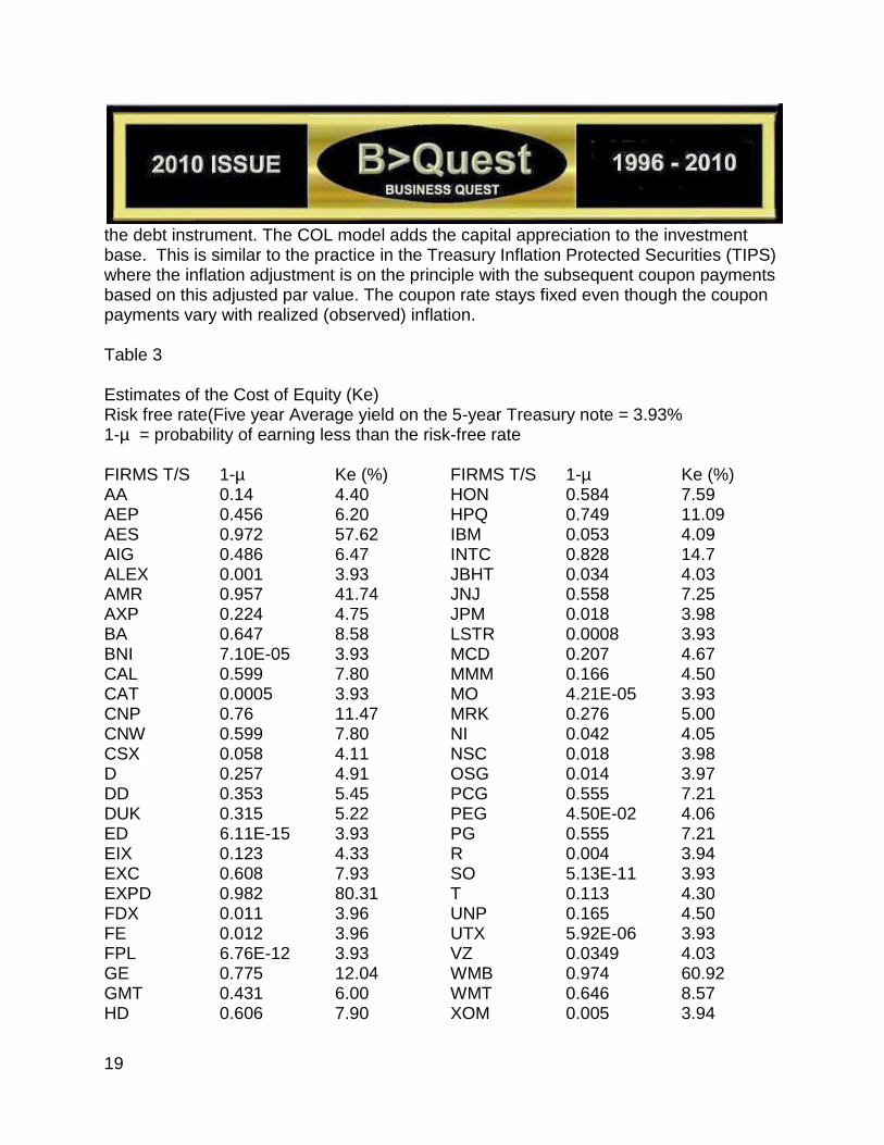
For the twenty-year estimation period, the results show a gamma value that increased in absolute value from 0.2254 for the three-year holding period to 0.4125 for the five-year holding period. This represents an 83 percent increase in risk averseness. For the ten-year holding period, the absolute value of gamma decreased significantly to 0.0055. This result is suspect because of the very high p-value (93.24 percent). For the three- and five-year holding periods, the results of the model are significant at the 4.5 percent and 0.01 percent levels, respectively. Over the twenty-year probability estimation period, the model explained 24.92% of the variation in the average five-year holding period returns with a p-value of 0.01% versus 7.72 percent for the three-year holding period with a p-value of 4.5 percent. This represents a more than tripling of the explanatory power of the model from a three-year to a five-year holding period. Neither the R-squared (0.015 percent) nor the p-value (93.24 percent) for the ten- year holding period return model is statistically significant. Table 3 below presents the estimates of the cost of equity for the sample firms used in the study. The results are consistent with the premise of the COL model. Although the results seem small compared to the returns usually reported on these firms, it is appropriate to point out that the realized returns on these firms‟ stock consist of income and capital gain. The capital gain is the expected net effect of new information on the magnitude, timing and risk of the expected cash flow on the present value the expected cash flow from owning the firm. Its effect on the period return is similar to the effect of interest rate and ratings changes on the period realized return on a debt instrument. This number can be significantly different from the yield to maturity of

19

the debt instrument. The COL model adds the capital appreciation to the investment base. This is similar to the practice in the Treasury Inflation Protected Securities (TIPS) where the inflation adjustment is on the principle with the subsequent coupon payments based on this adjusted par value. The coupon rate stays fixed even though the coupon payments vary with realized (observed) inflation. Table 3 Estimates of the Cost of Equity (Ke) Risk free rate(Five year Average yield on the 5-year Treasury note = 3.93% 1-µ = probability of earning less than the risk-free rate FIRMS T/S 1-µ Ke (%) FIRMS T/S 1-µ Ke (%) AA 0.14 4.40 HON 0.584 7.59 AEP 0.456 6.20 HPQ 0.749 11.09 AES 0.972 57.62 IBM 0.053 4.09 AIG 0.486 6.47 INTC 0.828 14.7 ALEX 0.001 3.93 JBHT 0.034 4.03 AMR 0.957 41.74 JNJ 0.558 7.25 AXP 0.224 4.75 JPM 0.018 3.98 BA 0.647 8.58 LSTR 0.0008 3.93 BNI 7.10E-05 3.93 MCD 0.207 4.67 CAL 0.599 7.80 MMM 0.166 4.50 CAT 0.0005 3.93 MO 4.21E-05 3.93 CNP 0.76 11.47 MRK 0.276 5.00 CNW 0.599 7.80 NI 0.042 4.05 CSX 0.058 4.11 NSC 0.018 3.98 D 0.257 4.91 OSG 0.014 3.97 DD 0.353 5.45 PCG 0.555 7.21 DUK 0.315 5.22 PEG 4.50E-02 4.06 ED 6.11E-15 3.93 PG 0.555 7.21 EIX 0.123 4.33 R 0.004 3.94 EXC 0.608 7.93 SO 5.13E-11 3.93 EXPD 0.982 80.31 T 0.113 4.30 FDX 0.011 3.96 UNP 0.165 4.50 FE 0.012 3.96 UTX 5.92E-06 3.93 FPL 6.76E-12 3.93 VZ 0.0349 4.03 GE 0.775 12.04 WMB 0.974 60.92 GMT 0.431 6.00 WMT 0.646 8.57 HD 0.606 7.90 XOM 0.005 3.94

20

Analysis and Conclusion In this paper, a model for estimating a firm‟s COE based on its earnings yield probability distribution about the risk-free rate of return is proposed. The model is centered on the concept that risk is defined as a chance of a loss and that if the chance of a loss is zero, the asset is considered risk free and the appropriate required return should be the risk-free rate. The chance of a loss is defined as the probability that the return from the investment will be less than the risk-free rate. The model uses the probability that the earnings yield on equity will be less than the risk-free rate as the determinant of the cost of equity. The lower this probability, the lower the required return on equity such that as this probability tends zero, the required return approaches the risk-free rate. Conversely, as the chance of a loss approaches unity, the required return tends to infinity. This is in line with the practical perception of risk.

This model is a marriage between the residual income valuation and the Fed E/P models. It recognizes the role of earnings yield as earnings of the owners of the business on the net amount invested in the business over the accounting period (where the value of their investment is measured by the stock price at the beginning of the period). If the firm‟s earnings yield is higher than the investors‟ required return, and is expected to remain higher, investors reward the owners by bidding up the value of the firm. This is consistent with observed market reaction to earnings announcement as described by Miller (2005) and Francis et al (2004) in their works on the role of “accrual quality” on the cost of equity.

The COL model also builds on the role of interest rates in security valuations by deriving the required ROE as a function of the risk-free rate. This is in line with Gode and Ohlson‟s (2004) study that documented the negative impact of increasing interest rate on the effect of earnings on security returns. Nissim and Penman (2003) finding that “the overall effect of changes in interest rates on equity value is negative, consistent with the negative correlation between changes in interest rates and stock returns”, lends additional support to this finding.

The COL model provides an alternative to the CAPM and the APT asset pricing

models and addresses the shortcomings inherent to both models. Unlike the CAPM and APT, the COL model does not rely on market/security return for its derivation. Instead, by using the variability of the earnings yield relative to the risk-free rate, it ties the required return to the firm‟s performance rather than the market reaction to the firm‟s performance, as implied by the CAPM and APT models. Most of all, it relies on

21

information that is readily available to investors. It is intuitive. It is not based on an undefined market portfolio and an expected return that are subject to forecasting error and bias. It addresses the limitation of the CAPM model as identified by Roll (1977) because it does not rely on the concept of a diversified portfolio, a situation that the CAPM assumes can be achieved with no transaction cost.

The COL model also contributes to the literature by providing a means of

evaluating and quantifying the average investor‟s or market risk tolerance level through the gamma exponent of the probability variable. The compliment of the probability variable is the chance of a loss, thus the exponent gamma reconciles the upside potential of the investment with the downside risk.

Finally, this is a theoretical model that is based on intuition and behavior of “rational and value maximizing” economic unit, a basic assumption in economic studies. This paper provides an empirical approach to the estimation of the cost of equity by allowing for a quantitative approximation of investor risk averseness. Based on this model, the cost of equity for a firm can be estimated as:

(6)

Where: Rq is the required return on equity of a firm RTB5 is the current yield on a five-year Treasury note μ is the probability that the earnings yield for the firm will be more than the yield

on the five-year Treasury note over a ten –year estimation period.

The 0.75 is a first approximation of 0.7513 value obtained for gamma using the five-year Treasury yield.

The residual of the regression model represents a measure of the abnormal or excess return earned over the investment horizon.Further work on this model is still necessary to determine its validity on a much broader market base. As a caveat, the results of this model cannot be compared to any of the models currently in use because of the fundamental difference in the definition of risk. The CAPM uses beta, which is the variability of the market return on a security relative to a market portfolio, as a measure of risk. The RIV and the constant growth dividend models calculate the internal rate of return as a proxy for the required return and do not explicitly consider the risk of the investment.

22

23

REFERENCES Alles, L., 1995, “Investment Risk Concepts and Measurement of Risk in Asset Returns,” Managerial Finance 21, (No.1), 15-25. Amoako-Adu, B. and B. Smith., 2002, “Analysis of P/E Ratios and Interest Rates”, Managerial Finance 28, (No. 4), 48-59. Anderson, K. and C. Brooks., 2005, “Decomposing the Price-Earnings Ratio,” Journal of Asset Management 6, (No. 6, July), 456-469. Anderson K. and C. Brooks., 2006, “The Long-Term Price-Earnings Ratio,” Journal of Business & Accounting 33, (No. 7 & 8, September/October), 1063-1066. Bali, Turan G., Nusret Cakici, and Yi Tang, 2009, “The Conditional Beta and The Cross-Section of Expected Returns”, Financial Management 38, (No. 1, Spring), 103-138. Beneda, N., 2002, “Growth Stocks Outperform Value Stocks Over the Long Term,” Journal of Asset Management 3, (No. 2, April), 112-123. Bhargava V. and D. Malhotra., 2006, “Do Price-Earnings Ratios Drive Stock Values?,” The Journal of Portfolio Management., 86-92. Borgman, R., and R. Strong, 2006, “Growth Rate and Implied Beta: Interactions of Cost of Capital Models,” Journal of Business and Economic Studies 12, (No.1), 1-10. Botosan, C., and M. Plumlee, 2005, “Assessing Alternative Proxies for the Expected Risk Premium,” The Accounting Review 80, (No.1), 21-53. Campbell, J.Y. and R.J. Shiller,1998, “Valuation Ratios and the Long-run Stock Market Outlook”, Journal of Portfolio Management 24, 11-26. Cheng, Q., 2005, “What Determines Residual Income?,” The Accounting Review 80, (No.1), 85-112. Constand, R., L. Freitas, and M. Sullivan., 1991, “Factors Affecting Price Earnings Ratios and Market Values of Japanese Firms,” Financial Management 20, (No. 4, Winter), 68-79.

24

Daske, H., G. Gebhardt, and S. Klein, 2006, “Estimating the Expected Cost of Equity Capital Using Analysts‟ Consensus Forecast,” Schmalenbach Business Review 58, (No.1), 2-36. Dunis, C. and D. Reilly., 2004, “ Alternative Valuation Techniques for Predicting UK Stock Returns,” Journal of Asset Management 5, (No.4, March), 230-250. Fama, E.F. and K.R. French, 1992, “The Cross-Section of Expected Stock Returns”, Journal of Finance 47, (No. 2), 427-465. Fisher, K. and M. Statman., 2006, “Marketing Timing Regressions and Reality,” The Journal of Financial Research 29, (No. 3, Fall), 293-304. Francis, J., R. LaFond, P. Olsson, and K. Schipper, 2004, “Costs of Equity and Earnings Attributes,” The Accounting Review 79, (No.4), 967-1010. Francis, J., K. Schipper, and L. Vincent, 2003, “The Relative and Incremental Explanatory Power of Earnings and Alternative (to Earnings) Performance Measures of Return,” Contemporary Accounting Research 20, (No.1), 121-164. Gode, D. and J. Ohlson, 2004, “Accounting-Based Valuation with Changing Interest Rates,” Review of Accounting Studies 9, 419-441. Lasher, William R., 2002, “Practical Financial Management,” Mason, Ohio: South-Western. Malkiel, B., 2004, “Models of Stock Market Predictability,” The Journal of Financial Research 27, (No. 4, Winter), 449-459. Megginson, W., 1997, “Corporate Finance Theory,” Reading, Massachusetts: Addison-Wesley. Miller, J., 2005, “Effects of Preannouncements on Analysts and Stock Price Reactions to Earnings News,” Review of Quantitative Finance and Accounting 24, 251-275. Miller, Kent D., and Michael J. Leiblein, 1996, “Corporate Risk-Return Relations: Returns Variability Versus Downside Risk,” Academy of Management Journal 39, No.1, 91-122.

25

Nissim, D., and S. Penman, 2003, “The Association Between Changes in Interest Rates, Earnings, and Equity Values,” Contemporary Accounting Research 20, (No.4), 775-804. Pindyck, R., and D. L. Rubinfeld, 1991, “Econometric Models & Economic Forecasts,” New York, NY: McGraw-Hill, Inc. Roll, R., 1977, “A Critique of the Assets Pricing Theory‟s Tests; Part I: On Past and Potential Testability of the Theory,” Journal of Financial Economics 4, 129-176. Ross, S., 1976, “The Arbitrage Theory of Capital Asset Pricing” Journal of Economic Theory 13, 341-360. Ross, S., 2006, “Fundamentals of Corporate Finance,” Boston, MA: McGraw-Hill Irwin. Rutterford, J., 2004, “From Dividend Yield to Discounted Cash Flow: A History of UK and US Equity Valuation Techniques,” Accounting, Business & Financial History 14, (No. 2, July), 115-149. Wei, S., and C. Zhang, 2006, “Why Did Individual Stocks Become More Volatile?,” The Journal of Business 79, (No.1), 259-292 Note: Title graphic is by Carole E. Scott