education production and incentives

Education Production and Incentives

Hugh MacartneyDuke University and NBER

Robert McMillanUniversity of Toronto and NBER

Uros PetronijevicYork University

September 2016

Introduction Context, Data and Variation Theory Contemporaneous Effects Persistence Effects Policy Implications Conclusion

• Many possible avenues for improving educational outcomes• increasing inputs, sharpening incentives, increasing competition

• We focus on particularly salient aspect of production: the teacher

• Sophisticated existing literature seeks to measure overall impactof teachers on student achievement

– Kane and Staiger (various); Chetty, Friedman and Rockoff (2014a,b)

• Separate literature measures effects of education accountability– Carnoy and Loeb (2002); Lavy (2002, 2009); Hanushek and Raymond (2005);

Dee and Jacob (2011); Imberman and Lovenheim (2015)

Macartney/McMillan/Petronijevic Education Production and Incentives


• We bring these two literatures together for the first time bydistinguishing between teacher effects that are

• invariant to prevailing incentives• responsive to them

• Convenient labels:• ‘teacher ability’

• incentive-invariant• e.g. experience, education, professional development• e.g. time-invariant teacher value-added

• ‘teacher effort’• any incentive-related action that raises scores• e.g. energy level and efficiency of delivery in classroom• e.g. preparation time for lessons outside classroom• e.g. degree of ‘teaching-to-the-test’



• Distinction allows us to address two key research questions:1 What are contemporaneous effects of teacher ability vs. teacher

effort in terms of student scores?2 What are persistent effects of teacher ability vs. teacher effort?

• identify extent of ‘teaching-to-the-test’

• Implications for policy: Focus on sharpening incentives orchanging teacher assignments?



• We develop a new empirical approach to distinguish betweenteacher ability and effort that exploits

• exogenous variation from well-known federal accountabilityscheme

• rich administrative data from North Carolina• all public school teachers and students over time



Our Approach

• To carry out contemporaneous decomposition (research question#1), implement three-step procedure that compares teachers

• who teach classrooms with higher versus lower fractions ofmarginal students

• before and after incentive reform was implemented

• To identify differential persistence (research question #2), carryout intuitive structural procedure that

• disentangles three sources of effort in year subsequent to reform’sintroduction



Preview of Results

Preview of Results: Effort Response

• School-level reform creates potent variation at teacher level• teacher value-added rises with incentive strength

• Evidence strongly suggests ‘teacher effort’ interpretation• reform does not cause school principals to re-sort teachers• nor does it cause them to alter class size

• Supporting evidence in literature:• Booher-Jennings (2005): survey shows Texas prototype caused

additional sessions and tutoring• Macartney (2016): U.S. teacher survey reveals reform led to

increase in additional hours worked



Preview of Results

Preview of Results: Effort Response

• Why no re-sorting of teachers across classes?• costly in short run, due to specific human capital (w.r.t. student

type)• pushback by parents of most able children

• Likely mechanism for teacher effort response:• school principals are effective managers and coordinate teachers

through pressure• undesirable reassignment may even be used as threat



Preview of Results

Preview of Results: Effects

• One SD increase in teacher ability (contemporaneously)equivalent to 0.18 SD test score increase

• One SD increase in teacher effort equivalent to 0.05 SD testscore increase

• Teacher ability has more persistent effect than teacher effort (butteacher effort does persist)

• 41 percent of initial teacher ability effect persists one year ahead• 13 percent for teacher effort



Relevance for Policy

Relevance for Policy

• Incentives matter when measuring teacher value-added• simply put, VA increases when incentives get stronger!

• Given that almost every jurisdiction in country hasaccountability, our findings inform the policy debate

• Implications for cost effectiveness of• sharpening incentives, vs.• altering distribution of teacher ability across classrooms and

schools

• proposed incentive-based reform is more cost-effective thanleading ability-based reform

• costs at least 12 percent less on per-teacher basis for samelong-run gain



Remainder of Talk

1 Introduction

2 Context, Data and Variation

3 Theory

4 Contemporaneous Effects

5 Persistence Effects

6 Policy Implications

7 Conclusion



Context and Data

• Take advantage of North Carolina policy backdrop and data

• NCLB system came into effect in 2003 on top of pre-existingstatewide ‘ABCs’

• NCLB: penalties for under-performing schools using fixed targets• ABCs: relatively uniform growth-oriented accountability scheme

that rewards educators based on value-added target

• Rich longitudinal administrative education data covering allpublic school students in North Carolina

• yearly student-level standardized test scores (1997-2005)• comparable across grades and years using developmental scale

• student, teacher and school characteristics• student: parental education, gender, race, disability, limited

English proficiency, free lunch eligibility



Incentive Variation

• Formal analysis of differential contemporaneous and persistenceeffects depends on establishing two related pieces of evidence:

1 NCLB induced an incentive response consistent with there beinga targeted effort increase predicted by standard theory

• identify marginal students by drawing upon our prior work• infers effort as a function of ex ante incentive strength using

exogenous NCLB-based variation

2 Teacher value-added is responsive to incentives

• We provide each piece of evidence, in turn, briefly reviewing theidentification procedure used for the first (from our prior work)



Identifying Incentive Response

• Identify marginal students as follows:

(i) Flexibly predict student performance using pre-reform data• regress ym

i,g,t=02 on cubic polynomial of prior math and readingscores f (yi,g−1,01) and student covariates Xi,g,02

• save coefficients

g−1

g

98 99 00 01 02 03

pre post





(ii) Construct ex ante incentive strength measure (y− yT )• predict performance y in 2003 using yi,g−1,02, Xi,g,03 and saved

coefficients

• given yT known, compute π ≡ y− yT

• measure does not include effort from heightened accountability

g−1

g

98 99 00 01 02 03

pre post





(iii) Given continuous incentive measure, semi-parametricallyuncover the underlying effort response function

• calculate difference between realized and predicted test score(y− y) for each level of π

g−1

g

98 99 00 01 02 03

pre post





(iv) Control: Repeat steps 1-3 using earlier pre-reform data• regress ym

i,g,99 on cubic polynomial of prior math and readingscores f (yi,g−1,98) and student covariates Xi,g,99

• save coefficients

g−1

g

98 99 00 01 02 03

pre(1st ed.)

pre(2nd ed.)

post





(iv) Control: Repeat steps 1-3 using earlier pre-reform data• predict performance y in 2000 using yi,g−1,99, Xi,g,00 and saved

coefficients

• compute π ≡ y− yT

• calculate difference between realized and predicted test score(y− y) for each level of π

g−1

g

98 99 00 01 02 03

pre(1st ed.)

pre(2nd ed.)

post





(v) Difference post- and pre-reform distributions to identify effortfunction


�



Incentive Strength and Test Score Response

-6-4

-20

24

68

10Sc

ore:

Rea

lized

- Pr

edic

ted

-22 -20 -18 -16 -14 -12 -10 -8 -6 -4 -2 0 2 4 6 8 10 12 14 16 18 20 22 24 26 28 30 32 34 36 38Score: Predicted - Target

Averages in 2003 Averages in 2000

95% CI in 2003 95% CI in 2000

Grade 4 Math


�



Estimated Effort Function

-4-2

02

Effo

rt

-12 -10 -8 -6 -4 -2 0 2 4 6 8 10 12 14 16 18 20 22 24 26 28 30 32 34Score: Predicted - Target

Parametric FitEffort Function



Linking to Teacher Value-Added

• Having shown how to identify marginal students (predictedperformance is close to the target), we now show that teachervalue-added depends on incentive strength

• Steps:• calculate fraction of marginal students within each classroom• estimate teacher-year fixed effects• plot teacher value-added against proportion marginal




Correlation Between Teacher VA and Proportion Marginal (Third Grade)

.51

1.5

Teac

her-Y

ear V

A

0 .2 .4 .6 .8 1Proportion of Marginal Students in Class




Correlation Between Teacher VA and Proportion Marginal (Fourth Grade)

23

45

6Te

ache

r-Yea

r VA





Correlation Between Teacher VA and Proportion Marginal (Fifth Grade)

11.

52

2.5

Teac

her-Y

ear V

A





• While this evidence strongly suggests that teachers respond toincentives, a more formal analysis is required to rule outalternative explanations:

• differential sorting of students to teachers• evolving teacher experience• random classroom shocks

• Our empirical strategy accounts for these factors, allowing us toseparately identify teacher ability and effort contemporaneously

• We then impose some structure to determine the extent to whicheffects persist differentially

• Simple theory to inform both approaches• only time for a brief overview



Main Elements

Main Elements

• Education production technology• cumulative with linear technology approximation• focus on both contemporaneous and dynamic effects of

unobserved teacher ability and effort



Main Elements

Main Elements

• Teacher effort decision, in light of accountability incentives• effort choice endogenous to prevailing incentive scheme• balance greater rewards against convex cost of effort• effort function depends on degree to which student is marginal

(under threshold targets)• effort unobserved, but identification approach to follow...



Main Elements

Main Elements

• Teacher assignment rule (taken as given)

• (Other aspects suppressed:• student effort• student peer effects• parental help ...)



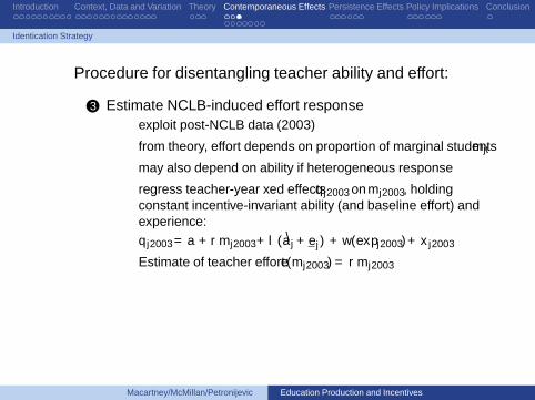
Identification Strategy

• Procedure for disentangling teacher ability and effort:

1 Compute teacher-year fixed effects from 1997 to 2005 (q jt )• in keeping with existing approaches taken in literature, use

grade-specific regressions of contemporaneous scores on cubics inprior scores, teacher fixed effects and other student covariates

• each fixed effect is sum of ability, effort and classroom shock:q jt = a j + e j +1nclbe jt(m jt)+ ε jt

where m jt is the proportion of marginal students (close to NCLBproficiency cutoff) taught by teacher j in year t, and e j ispre-existing baseline ABCs effort





2 Estimate incentive-invariant ability and baseline effort• exploit data prior to NCLB response

• conditional on teacher experience, assume fixed over time

• employ Empirical Bayes estimator of teacher value-added toseparate out teacher ability and baseline effort fromclassroom-specific shocks and student-level noise, recovering theestimate (a j + e j)





3 Estimate NCLB-induced effort response• exploit post-NCLB data (2003)

• from theory, effort depends on proportion of marginal students m jt

• may also depend on ability if heterogeneous response

• regress teacher-year fixed effects q j2003 on m j2003, holdingconstant incentive-invariant ability (and baseline effort) andexperience:q j2003 = α +ρm j2003 +λ (a j + e j) +w(exp j2003)+ξ j2003

• Estimate of teacher effort: e(m j2003) = ρm j2003



Empirical Results

• Incentive-invariant ability across all teachers (pre-reform data)• µa =−0.07 and σa = 0.18 student-level SDs

0.0

5.1

.15

.2.2

5.3

.35

Den

sity

-15 -10 -5 0 5 10 15EB Estimated Ability (Measured in Developmental Scale Points)

kernel = epanechnikov, bandwidth = 0.1722

Incentive-Invariant Ability

All Teachers



Empirical Results

• Similar distributions across all grade levels• Third grade: µa =−0.07 and σa = 0.20 student-level SDs

0.0

5.1

.15

.2.2

5.3

.35

Den

sity




Third Grade Teachers



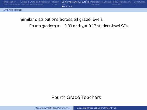
Empirical Results

• Similar distributions across all grade levels• Fourth grade: µa =−0.09 and σa = 0.17 student-level SDs

0.0

5.1

.15

.2.2

5.3

.35

Den

sity




Fourth Grade Teachers



Empirical Results

• Similar distributions across all grade levels• Fifth grade: µa =−0.06 and σa = 0.17 student-level SDs

0.0

5.1

.15

.2.2

5.3

.35

Den

sity




Fifth Grade Teachers



Empirical Results

• Now set out to uncover effort distributions by grade and overall

• To do so, first show that teacher productivity systematicallydepends on NCLB incentives

• recall: marginal students receive largest amount of NCLB effort• conditional on teacher ability, teacher-year effect should be

increasing in fraction of marginal students in classroom (m jt )

• Find clear positive relationship in 2003, but not pre-reform years



Empirical Results

• Teacher-year effect vs. m jt in third grade• 1 SD increase in m jt ⇒ 0.03 student-level SD increase in scores

-.50

.51

1.5

2Te

ache

r-Yea

r VA

-.5 -.2 .1 .4 .7 1Residual Proportion of Marginal Students in Class

2003 (1998 - 2000) & 2002

Teacher-Year VA vs. Proportion of Marginal Students in Class




Empirical Results

• Teacher-year effect vs. m jt in fourth grade• 1 SD increase in m jt ⇒ 0.06 student-level SD increase in scores

-20

24

6Te

ache

r-Yea

r VA


2003 1998 - 2001





Empirical Results

• Teacher-year effect vs. m jt in fifth grade• 1 SD increase in m jt ⇒ 0.04 student-level SD increase in scores

01

23

4Te

ache

r-Yea

r VA


2003 1998 - 2001





Empirical Results

• Approach for recovering effort exploits comparisons betweenteachers with varying proportions of marginal students over time

• To strengthen causal claim, we estimate analogous relationshipbetween change in teacher-year effects (q jt − q jt−1) and m jt foreach grade

• in contrast to level-based analysis, only exploits within-teachervariation

• results indicate that effect is driven by individual teachersresponding to incentives: change-based coefficients arestatistically indistinguishable from level-based counterparts



Empirical Results

• q jt − q jt−1 vs. m jt in third grade

-10

12

3D

iffer

ence

in T

each

er V

A

-.5 0 .5 1Residual Proportion of Marginal Students in Classroom

2003 2000

Performance Improvement vs. Proportion Marginal




Empirical Results

• q jt − q jt−1 vs. m jt in fourth grade

02

46

Diff

eren

ce in

Tea

cher

VA

-.2 0 .2 .4 .6 .8Residual Proportion of Marginal Students in Classroom

2003 2000





Empirical Results

• q jt − q jt−1 vs. m jt in fifth grade

-10

12

3D

iffer

ence

in T

each

er V

A

-.5 0 .5 1Residual Proportion of Marginal Students in Classroom

2003 2000





Empirical Results

• Effort interpretation requires ruling out most plausible rivalhypothesis:

• re-sorting of teachers by principals due to NCLB in 2003

• Such re-sorting could lead estimate to be driven by change inrelationship between m jt and teacher ability (rather than effort)

• Rule out hypothesis by regressing m jt on ability and abilityinteracted with post-reform indicator

• coefficient on interacted term is either indistinguishable from zeroor slightly negative

• slight sorting change in 2003 leads high-ability teachers toreceive smaller fractions of marginal students (opposite direction)

• Significant non-interacted coefficient reveals significantpre-reform heterogeneity

• justifies ability control in main specification



Empirical Results

• Also reveals effort response and ability are negatively correlated

• Using m jt in 2003 and pre-reform teacher ability estimates,adjust for correlation to compute distribution of effort:

0.5

11.

5D

ensi

ty

0 .5 1 1.5 2 2.5 3 3.5 4 4.5NCLB Effort (Measured in Developmental Scale Points)


Effort Distribution

Third Grade

0.5

11.

5D

ensi

ty



Effort Distribution

Fourth Grade

0.5

11.

5D

ensi

ty



Effort Distribution

Fifth Grade

• Across grades:• average effort is 0.61 scale points• SD of effort is 0.48 scale points (0.05 student-level SDs)



Overview

• Now use measures of teacher ability and effort to investigateextent to which each input persists in determining future scores

• novel in that literature providing persuasive evidence of long-runeffects of conventional teacher quality measures (e.g. Chetty etal. 2014b) does not allow a role for incentives

• Two parts:1 Estimating persistence of teacher ability2 Estimating persistence of teacher effort

• Discuss each in turn



Teacher Ability

Estimating Persistence of Teacher Ability (and Baseline Effort)

• Rely on pre-NCLB data and methods used previously in the literature:regress future scores on standard VA control variables and ourmeasures of teacher incentive-invariant ability

• Find 0.41 remains after one year and 0.19 after four– in line with Jacob, Lefgren and Sims (2010); Chetty et al. (2014a)

0.2

.4.6

.81

Effe

ct o

n M

ath

Scor

e

-2 -1 0 1 2 3 4Years Removed from Year t Teacher

Test Score Effect 95 Percent CI

Pre-NCLB Data: 1997 to 2002Persistence of Teacher Ability and Baseline Effort



Teacher Effort

Estimating Persistence of Teacher Effort

• Much more challenging

• Ideal experiment for cleanly identifying persistent effects ofNCLB-related effort shock in 2003:

• repeal both NCLB and ABCs in 2004 and beyond• in that case, no future effort decisions would be made• thus, would be able to estimate how effort levels from 2003

(already estimated in first part) persisted using regressionapproach

• In practice, both accountability schemes continued to operate• as consequence, educators faced two contemporaneous effort

decisions in each period after NCLB’s introduction• each affects contemporaneous test scores while also being

correlated with initial effort response in 2003



Teacher Effort


• Under NCLB:• prior and contemporaneous effort decisions tend to exhibit strong

within-student correlations over time• why? students predicted to be on the margin of passing in one

year also likely to be close the next

• Under ABCs:• targets set at school level and depend on students’ prior scores

• implies that any effort responses affecting test scores in one periodalso affect ABCs targets the next

• so initial response to heightened NCLB incentives would increaseschools’ future ABCs targets on average

• making it more difficult to pass• potentially causing schools to modify their effort decisions



Teacher Effort


• We use our model to develop a structural estimation approach• controls for contemporaneous test score effects stemming from

the two ongoing programs while estimating the persistence ofeffort from 2003

• accounts for fact that contemporaneous NCLB effort is a functionof persistence effect we are trying to estimate

• under proficiency-count system, effort decision depends onproximity of target to students’ expected scores in absence ofadditional effort

• but students’ predicted scores depend on degree to which prioreffort persists forward, making contemporaneous effort decisions afunction of persistence rate

• parameter governing the persistence of effort thus has to beestimated structurally, as one regressor (contemporaneous effort) isinherently a function of main parameter of interest



Teacher Effort


• Results:• structural estimates of the persistence of effort reveal that 13

percent of initial effort persists one period forward• amounts to approximately 32 percent of one-year persistence of

teacher ability (0.41)• ignoring contemporaneous effort decisions would result in

overestimate of persistence rate of effort (50 vs. 13 percent)

• faster decay for effort relative to ability in line with teachers‘teaching-to-the-test’ to some degree

• phenomenon often discussed but rarely identified empirically• fact that portion of prior effort carries over in scores suggests that

effort does have longer-term benefits



• Our analysis is relevant to recent education policy discussions

• Focus has been on altering distribution of teacher ability• increasing teacher ability can involve firing lowest rated or

reducing attrition rate of highest rated• Chetty et al. (2014b) argue former more cost-effective• firing bottom 5 percent of teachers results in average 2 SD higher

ability draw for that subset• requires additional compensation for increased employment risk:

estimated mean salary increase of 1.4 percent to equilibrateteacher labor market (Rothstein 2013)

• Alternative for improving student performance: incentive reform• our framework and findings are well suited to evaluating cost

effectiveness of leading ability- and effort-oriented policies



• Can raise teacher productivity by equivalent 2 SD throughNCLB target refinement

• non-marginal students with predicted performance above existingtarget: ∼ 60%

• from estimates, costlessly making them marginal through toughertargets increases effort by one SD of ability

• 26% already marginal under existing targets• so 86% marginal under refinement: 1.43 SD of ability effect• raise value of sanction to 140% of existing: 2 SD of ability• but while effort-based benefit applies to all teachers,

ability-reform only applies to bottom 5 percent at increased salarycost of $700 (i.e. $50,000×0.014) for all teachers

• so scale 140% sanction to reflect comparable improvement: 7%of existing value



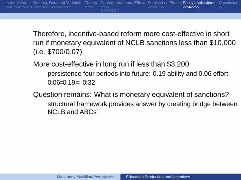
• Therefore, incentive-based reform more cost-effective in shortrun if monetary equivalent of NCLB sanctions less than $10,000(i.e. $700/0.07)

• More cost-effective in long run if less than $3,200• persistence four periods into future: 0.19 ability and 0.06 effort• 0.06/0.19 = 0.32

• Question remains: What is monetary equivalent of sanctions?• structural framework provides answer by creating bridge between

NCLB and ABCs



• To determine monetary equivalent, we:• calculate degree to which schools lowered probability of passing

ABCs in 2004 by responding to NCLB in 2003 (relative tocounterfactual scenario in which NCLB never enacted), varyingimportance of noise (relative to effort) under ABCs

• calculate expected financial loss for each school from NCLBresponse, using difference in passing probabilities and ABCsbonus payment of $1,500 per teacher

• combine expected loss with estimate of how school-level effortresponds to changes in ABCs targets



• Findings:• depending on noise, one unit increase in 2003 NCLB effort

reduces probability of passing ABCs by between 8 and 19percentage points

• expected financial loss for teacher in average school between$120 and $435

• based on relationship between ABCs effort and target, $1expected financial loss under ABCs causes increase in test scoresof between 0.007 and 0.0025 scale points

• average school-level NCLB effort gain in 2003: 1.96 scale points• therefore, NCLB sanction valued between $784 (i.e. 1.96/0.0025)

and $2,800 (i.e. 1.96/0.0007)



• Upper-bound value of NCLB sanction: $2,800• assuming chance plays very large role in outcome

• Lower than both $10,000 (SR) and $3,200 (LR)• incentive-based reform more cost-effective than ability-based

counterpart

• Put another way, per-teacher sanction amount is 87.5 percent($612.50) of $700 ability cost

• Even more cost-effective, considering incentives can affect effortdecisions of all teachers

• ability reform limited in this regard



• Outlined new empirical strategy allowing us to• separate out teacher effort from teacher ability• explore their differential persistence

• Findings:• evidence strongly suggests effort response by teachers• one SD increase in ability and effort contemporaneously raises

test scores by 0.18 SD and 0.05 SD, respectively• showed teacher effort less persistent than ability

• but still positive impact – sheds light on ‘teaching-to-the-test’debate

• Relevant for decision to use incentive measures versus teacherreassignments (or firing)

• proposed incentive-based reform is more cost-effective thanleading ability-based reform


�

Validity: No Bunching at Target

0.0

1.0

2.0

3.0

4.0

5.0

6D

ensi

ty

-10 0 10 20 30 40Score: Predicted - Target

Grade 4 Math in 2003


�

Test Score Response

2000 2003

0.0

2.0

4.0

6.0

8.1

Den

sity

-30 -25 -20 -15 -10 -5 0 5 10 15 20 25 30Score: Realized - Predicted

Grade 4 Math


education production and incentives

Documents