effect of rainfall events on the thermal and moisture

University of VermontScholarWorks @ UVM

Graduate College Dissertations and Theses Dissertations and Theses

2015

Effect Of Rainfall Events On The Thermal AndMoisture Exposure Of Underground ElectricCablesAndrew FuhrmannUniversity of Vermont

Follow this and additional works at: https://scholarworks.uvm.edu/graddis

Part of the Mechanical Engineering Commons, and the Soil Science Commons

This Thesis is brought to you for free and open access by the Dissertations and Theses at ScholarWorks @ UVM. It has been accepted for inclusion inGraduate College Dissertations and Theses by an authorized administrator of ScholarWorks @ UVM. For more information, please [email protected].

Recommended CitationFuhrmann, Andrew, "Effect Of Rainfall Events On The Thermal And Moisture Exposure Of Underground Electric Cables" (2015).Graduate College Dissertations and Theses. 331.https://scholarworks.uvm.edu/graddis/331

https://scholarworks.uvm.edu?utm_source=scholarworks.uvm.edu%2Fgraddis%2F331&utm_medium=PDF&utm_campaign=PDFCoverPages

https://scholarworks.uvm.edu/graddis?utm_source=scholarworks.uvm.edu%2Fgraddis%2F331&utm_medium=PDF&utm_campaign=PDFCoverPages

https://scholarworks.uvm.edu/etds?utm_source=scholarworks.uvm.edu%2Fgraddis%2F331&utm_medium=PDF&utm_campaign=PDFCoverPages

https://scholarworks.uvm.edu/graddis?utm_source=scholarworks.uvm.edu%2Fgraddis%2F331&utm_medium=PDF&utm_campaign=PDFCoverPages

http://network.bepress.com/hgg/discipline/293?utm_source=scholarworks.uvm.edu%2Fgraddis%2F331&utm_medium=PDF&utm_campaign=PDFCoverPages

http://network.bepress.com/hgg/discipline/163?utm_source=scholarworks.uvm.edu%2Fgraddis%2F331&utm_medium=PDF&utm_campaign=PDFCoverPages

https://scholarworks.uvm.edu/graddis/331?utm_source=scholarworks.uvm.edu%2Fgraddis%2F331&utm_medium=PDF&utm_campaign=PDFCoverPages

mailto:[email protected]

EFFECT OF RAINFALL EVENTS ON THE THERMAL AND MOISTURE EXPOSURE OF UNDERGROUND ELECTRIC CABLES

A Thesis Presented

by

Andrew Fuhrmann

to

The Faculty of the Graduate College

of

The University of Vermont

In Partial Fulfillment of the Requirements for the Degree of Master of Science

Specializing in Mechanical Engineering

May, 2015

Defense Date: December 10, 2014 Thesis Examination Committee:

Jeffrey S. Marshall, Ph.D., Advisor George Pinder, Ph.D., Chairperson

William Louisos, Ph.D. Cynthia J. Forehand, Ph.D., Dean of Graduate College

ABSTRACT

Cable ampacity analysis is generally performed assuming constant worst-state environmental conditions, which often correspond to a dry soil condition or to a condition with uniform ambient soil moisture content. The characteristic time scale of thermal variation in the soil is large, on the order of several weeks, and is similar to the time scale between rainfall events in many geographic locations. Intermittent rainfall events introduce significant transient fluctuations that influence the thermal conditions and moisture content around a buried cable both by increasing thermal conductivity of the soil and by increasing the moisture exposure of the cable insulation. This paper reports on a computational study of the effect of rainfall events on the thermal and moisture transients surrounding a buried cable. The computations were performed with a finite-difference method using an overset grid approach, with an inner polar grid surrounding the cable and an outer Cartesian grid. The thermal and moisture transients observed in computations with periodic rainfall events were compared to control computations with a steady uniform rainfall. Under periodic rainfall conditions, the temperature and moisture fields are observed to approach a limit-cycle condition in which the cable surface temperature and moisture content oscillate in time, but with mean values that are significantly different than the steady-state values.

ii

CITATION

Material from this thesis has been accepted for publication in the International Journal of

Heat and Mass Transfer on September 26, 2014 in the following form:

J.S. Marshall and A.P. Fuhrmann.. “Effect of rainfall transients on thermal and moisture

exposure of underground electric cables,” Int. Journal of Heat and Mass Transfer,

vol. 80, pp. 660-672, 2015.

iii

ACKOWLEDGEMENTS

I would like to give a very special thanks to my professor, mentor, and advisor, Dr.

Jeffrey Marshall. I am so grateful for all of the knowledge you have given me as my

professor, and for guiding me into the field of Fluid Dynamics, where I have found my

passion. Your classes and teaching method have been challenging, thorough, and

consistently rewarding. As my advisor, you provided me many opportunities to further

my education and take on new challenges, and were always available to assist me.

Finally, I’d like to thank you for being so patient, understanding, and supportive when an

injury postponed my graduate research. I have a great respect for you.

I’d also like to thank Dr. William Louisos and Dr. George Pinder for their participation

on my thesis committee, and for the knowledge they imparted on me as professors, which

prepared me for this research and all future engineering work.

I am so fortunate to have shared a graduate lab space with intelligent, friendly, and

helpful students. A big thank you to Chris Ghazi, Adam Green, Melissa Faletra, Simtha

Sankaran, Kyle Sala, and Ian Pond for all the camaraderie through the past few years.

The community we built was so comforting whenever the work became stressful, and it

seemed as though our combined knowledge could solve any engineering problem.

This work was sponsored by the U.S. Dept. of Transportation, through the University of

Vermont Transportation Research Center (grant TRC039), and by the National Science

Foundation (grant DGE-1144388).

iv

TABLE OF CONTENTS

Page

CITATIONS……………………………………………………………………………. ii

ACKNOWLEDGEMENTS……………………………………………………………. iii

LIST OF TABLES……………………………………………………………………… vi

LIST OF FIGURES…………………………………………………………………….. vii

CHAPTER 1: INTRODUCTION………………………………………………………. 1

1.1. Motivation…………………………………….………………………………….. 1

1.2. Objective and Scope……………………………………………………………… 5

1.3. Thesis Overview………………………………………………………………….. 6

CHAPTER 2: REVIEW OF LITERATURE……………………………………………. 7

2.1. Rainfall Infiltration into Soil……………………………………………………… 7

2.2. Heat Transfer Around Power Cables in Soil……………………………….……. 13

2.2.1. Thermal Conductivity……………………………………………………….. 13

2.2.2. Analytical Methods………………………………………………………….. 14

2.2.3. Numerical Methods………………………………………………………….. 16

2.3. Coupled Heat and Moisture Transfer in Soil……………………………………. 18

2.3.1. Numerical Methods…………………………………………….……………. 19

2.3.2. Experimental Methods……………………………………………………… 22

CHAPTER 3: THEORY AND METHOD…………………………………………….. 24

3.1. Governing Equations …………………………………………………………… 24

3.1.1. Coupled Heat and Moisture Transfer Equations……………………………. 24

3.1.2. Coefficient Definitions……………………………………………………… 26

3.2. Computational Method………………………………………………………….. 28

v

3.2.1. Assumptions and Limitations………………………………………….……. 28

3.2.2. Computational Domain and Boundary Conditions…………….……….…… 30

3.2.3. Overset Grids………………………………………………….………….…. 32

3.3.4. Numerical Method…………………………………………….………….…. 33

3.3.5. Dimensionless Parameters…………………………………….………….…. 34

3.3.6. Grid Independence and Validation…………………………….………….… 37

CHAPTER 4: RESULTS AND DISCUSSION………………………….………….…. 43

4.1. Initialization……………………………………………………….………….…. 43

4.1.1. Finding the Steady State Moisture Field……………………….………….… 43

4.1.2. Finding the Steady State of Coupled Temperature and Moisture Field…..…. 45

4.2. Periodic Variation of Rainfall Intensity, Duration, and Frequency…………..….. 49

CHAPTER 5: CONCLUSIONS AND FUTURE WORK………………………….….. 64

5.1. Conclusions………………………………………………………………….…... 64

5.2. Applications and Future Work…………………………………………………... 66

REFERENCES………………………………………………………………………… 68

vi

LIST OF TABLES

Page

Table 1. Expressions used for the variable coefficients that characterize heat and moisture transport in the soil as functions of temperature T (in degrees Kelvin) and relative moisture content satS θθ /≡ . The different

coefficients are in SI units, as indicated in the nomenclature section…………...………28 Table 2. List of dimensionless parameters whose values are held fixed, and their values in the current computations…………………………………………….37 Table 3. Number of points in different grids used in grid independence study…………………………………………………………………………………..….45 Table 4. Listing of rainfall conditions used for periodic rainfall computations in conditions typical of dry and moist climates. Rainfall is characterized by the dimensionless rainfall intensity 0/ θKQQ rainrain =′ ,

duration LRrainD ττ /= , and frequency Lff τ=′ . The computational

results are listed for the change in the mean values of dimensionless temperature and moisture content from the steady-state solutions, surfT ′∆

and surfθ∆ , and the oscillation amplitude of the dimensionless temperature

and moisture content in the periodic solution, ampT ′ and ampθ …………………...……….53

vii

LIST OF FIGURES

Page

Figure 1. Infiltration curves for different rainfall intensities I1, I2, I3, and I4, where KS is the saturated hydraulic conductivity [Mein and Larson, 1971]…………….10 Figure 2. A typical moisture content profile at the moment of surface saturation, where θi represents the initial moisture content and θs represents the saturated moisture content [Mein and Larson, 1971]…………………….12 Figure 3. The assumed moisture content profile some time after the surface has saturated and the wetting front has propagated downward, where θi represents the initial moisture content and θs represents the saturated moisture content [Mein and Larson, 1971]……………………………………12 Figure 4. Close-up figures showing (a) overlapping inner grid surrounding each cable and the outer Cartesian grid and (b) fringe points of the outer grid (open circles) and inner grid (filled circles). In (b), outer grid cells that overlap the outer boundary of the inner grid are shaded gray. [Marshall et al., 2013]……………………………………………………………………18 Figure 5. Variation of cable temperature for uniform and progressive cyclic load for a sandy silt soil with an initial moisture content value of 0.35 [Freitas and Prata, 1996]…………………………………………………………...20 Figure 6. Temperatures at surface of the outer cable for the directly buried cable experiments for measured data (dash-dot), heat/moisture program results (dashed), and heat only program results (solid) [Anders and Radhakrishna, 1988]…………………………………………………………………….21 Figure 7. Plot of the effective thermal conductivity of soil used in the computations as a function of moisture content…………………………………………27 Figure 8. Schematic diagram of the computational flow domain and the inner (polar) and outer (Cartesian) grids, where the cable is identified as a black circle at the center of the inner grid, which is submerged a depth b below the ground. The boundaries of the outer grid are identified by circled numbers…………………………………………………………………………..31 Figure 9. Time variation of the average cable surface temperature and moisture content for the grid independence study, for grids A (dash-dot), B (solid), and C (dashed)………………………………………………………………. .39

viii

Figure 10. Comparison of predicted dimensionless average cable surface temperature for a case with the thermal convection term (solid line) and without the thermal convection term (dashed line) for the same run as shown in Figure 3……………………………………………………………...…………40 Figure 11: Comparison of the one-dimensional moisture content value over a 12 hour rainstorm of intensity 0.8 between (a) the current model and (b) the CHEMFLO-2000 commercial software……………………………..………42 Figure 12. Steady-state moisture content profiles for cases with (A)

03.0=′rainQ , (B) 0.02, (C) 0.01, (D) 0.005, and (E) 0 as a function of

dimensionless depth ξ . The initial moisture profile in the calculations is indicated by a dashed line. For the case with no rain, the moisture content moves downward very slowly in time and no steady-state profile is observed. The moisture profile shown in E is plotted at a time of approximately 10 years after the initial condition. The other cases have all converged to steady-state profiles within four significant figures in the moisture content………………………………………………………………….………44 Figure 13. Time variation of the average cable surface (a) temperature and (b) moisture content during the second preliminary computation for cases with (A) 03.0=′rainQ , (B) 0.02, (C) 0.01, and (D) 0.005. In (a), the

dimensionless temperature is shown on the left-hand y-axis and the corresponding change in dimensional temperature for the example problem is shown on the right-hand y-axis. The figure shows the approach of the temperature and moisture content fields to a steady state condition………….…..46 Figure 14. Steady-state (a) dimensionless temperature and (b) moisture content fields at the end of the second preliminary computation for the case with 03.0=′rainQ ……………………………………………………………...…….48

Figure 15. Variation of (a) temperature and (b) moisture content on the line 0=′x as a function of dimensionless depth ξ for the same four

values of rainQ ′ shown in Figure 6. In (a), the dimensionless temperature is

shown on the left-hand y-axis and the corresponding change in dimensional temperature for the example problem is shown on the right- hand y-axis……………………………………………………………………………….49 Figure 16. Oscillation of average dimensionless temperature and moisture content on the cable surface as functions of dimensionless time with constant cable heat flux, for Run D1. The oscillations observed in the plots are due to periodic rain events. In (a), the dimensionless temperature is

ix

shown on the left-hand y-axis and the corresponding change in dimensional temperature for the example problem is shown on the right- hand y-axis……………………………………………………………………………….54 Figure 17. Plot of dimensionless cable surface temperature as a function of cable surface moisture content for Run D1, showing the approach of the system to a limit-cycle behavior at long time……………………………………………54 Figure 18. Variation of (a) dimensionless temperature and (b) moisture content on the line 0=′x as a function of the dimensionless depth ξ for Run D1 at times (A) =′t 575.2, (B) 575.4, (C) 575.8, (D) 577.2, (E) 583.6, and (F) 575 and 600. The same six lines are plotted in (a), but the curves nearly overlap. In (a), the dimensionless temperature is shown on the left-hand y-axis and the corresponding change in dimensional temperature for the example problem is shown on the right-hand y-axis………………………….…..….55 Figure 19. Contour plot of the moisture content for a time interval of one day following a rain storm, for Run D1. The plots are made at dimensionless times (a) 575=′t , (b) 575.2, (c) 575.4, (d) 575.6, (e) 575.8, and (f) 576………………………………………………………………………………..59 Figure 20. Oscillation of average dimensionless temperature and moisture content on the cable surface as functions of dimensionless time with constant cable heat flux, for Run M1. The oscillations observed in the plots are due to periodic rain events. In (a), the dimensionless temperature is shown on the left-hand y-axis and the corresponding change in dimensional temperature for the example problem is shown on the right- hand y-axis……………………………………………………………………………….60 Figure 21. Variation of (a) dimensionless temperature and (b) moisture content on the line 0=′x as a function of the dimensionless depth ξ for Run M1 at times (A) =′t 587.6, (B) 587.8, (C) 588.0, (D) 588.4, and (E) 590.0, and (F) 587.5 and 600. The same six lines are plotted in (a), but they nearly overlap. In (a), the dimensionless temperature is shown on the left-hand y-axis and the corresponding change in dimensional temperature for the example problem is shown on the right-hand y-axis……………………………..60 Figure 22. Amplitude of average cable surface (a) dimensionless temperature and (b) moisture content fluctuations with periodic rain events as functions of dimensionless rain frequency. Results are for the moist condition (triangles, dashed line) and the dry condition (circles, solid line) listed in Table 4. The curves are exponential fits to the data. In (a), the dimensionless temperature is shown on the left-hand y-axis and the corresponding change in dimensional temperature for the example

x

Page

problem is shown on the right-hand y-axis……………………………………………....63 Figure 23. Change in mean values of the average cable surface (a) dimensionless temperature and (b) moisture content with periodic rain events as functions of dimensionless rain frequency. Results are for the moist condition (triangles, dashed line) and the dry condition (circles, solid line) listed in Table 4. The curves are exponential fits to the data. In (a), the dimensionless temperature is shown on the left-hand y-axis and the corresponding change in dimensional temperature for the example problem is shown on the right-hand y-axis………………………………………...…….63

1

CHAPTER 1: INTRODUCTION

1.1 Motivation

There is an increasingly urgent need to improve America’s power delivery

infrastructure to accommodate for changing energy needs and new sustainability

expectations. Current standards and regulations are based on an outdated model that may

over- or under-restrict the amount of energy that can be safely sent through the cables in

different areas of the country. These regulations exist because the system of underground

power cables are subject to a variety of hazards that could compromise their efficiency

and lifespan, such as electrical overloading, thermal degradation, and moisture

penetration. As electrical current flows through the power cables, heat is generated and

released by the cable. It is desirable to encourage the heat to dissipate away from the

cable and into the surrounding soil to avoid issues of overheating that can damage the

cable insulation. Additionally, overheating has an adverse effect on the efficiency of

power delivery. The operating temperature of the cable is directly related to the current-

carrying capacity, so under favorable heat transfer conditions, and therefore lower

operating temperatures, the power delivery is more efficient and smaller-sized cables can

sustain higher currents without overheating [Freitas and Prata, 1996].

It is predicted that the stresses on the electric-power delivery system will increase in

future years. A movement away from coal and natural gas, and towards renewable

energy, will result in an increased load and overall usage of the electric grid.

Additionally, new technologies available for residential use and an increased dependency

2

on electronics will further increase the load to which the cables are subjected. One such

technology that is growing in popularity is the electric vehicle. Charging electric vehicles

require a load that is much larger than that required by typical household appliances, and

can add significant stress to the power delivery cables and transformers. The stresses will

increase in the near future as predictions expect an increase of plug-in electric vehicles

(PEV’s) to the transportation market [Fernández et al., 2011]. To make matters more

difficult, there will often be a localized, high density of PEV owners due to factors such

as charging infrastructure locations as well as social and media influences [Eppstein et

al., 2011] that will result in electric loads much higher than that expected based on

national averages. In preparation for these increased demands on the electric grid, there is

both environmental and financial motivation for understanding how a power cable will

respond to the new electrical and environmental stresses that it may encounter.

Water moisture within the soil poses a threat to the structural integrity of the cables

as well. If the buried cables are over-exposed to moisture, then they are susceptible to

insulation degradation. This damaging process is known as water treeing, which is the

penetration of water into the hydrophobic cable insulation that occurs when the insulation

is exposed to a combination of moisture and electrical stress. Formation of water trees

can take years, but once formed, the deteriorating impact they have on the insulation is

significant and can severely compromise the efficiency of the power delivery. An

indirect, though very important, effect of the moisture content in the soil is its effects on

the heat transfer properties around the cable. The ability to dissipate heat away from the

cable depends on the physical properties of the surrounding medium, of which the most

3

important is the thermal conductivity [Anders and Radhakrishna, 1988]. The thermal

conductivity itself is a function of several properties, including moisture content,

temperature, and other physical and geometric characteristics of the soil. Even so,

conductivity is most sensitive to moisture content [Deru, 2003], which will cause

increased thermal conductivity as the moisture content rises. Under certain thermal

conditions, all of the moisture may be forced away from the cable by the thermal

gradients, creating a drier zone surrounding the cable. The possible formation of the dry

zone is vital to consider when forming a thermal model of an underground cable because

thermal conductivity of soil can decrease by over a factor of three when dry, allowing a

sharp rise in temperature than could damage the buried cable [Anders and Radhakrishna,

1988]. Additionally, once a dry zone is formed, the sharp increase of temperature will

further increase the size of the dry zone and result in a self-propagating scenario, possibly

leading to a thermal runaway and the destruction of the cable insulation. Therefore,

moisture content in the soil is an interesting and important aspect to study. Moisture

content values that are too high or too low can lead to cable damage, while a moderate

value can be highly beneficial due to its favorable thermal mitigation effects. The effects

of moisture distribution and transfer are not only important for predicting the onset of

water treeing in the insulation, but also are vital in creating an accurate model of the heat

transfer processes around the cable.

There is a need for the development of an accurate and realistic model that predicts

the thermal and fluid behavior around a loaded cable in order to gain insight on how to

improve the power delivery infrastructure. Many thermal models of underground cables

4

already exist that accurately characterize the heat and moisture transfer around a heated

cable under certain, strict conditions. Many of these models focus only on a scenario

where both the heat and moisture fields have reached a steady state, whereas a few

studies have considered transient heat and moisture transfer under constant environmental

conditions. However, these models do not include an important phenomenon that may

render the steady state model as unrealistic − rain. Rainfall events have a significant

impact on the soil moisture content, and therefore also the soil thermal properties. In most

cases, rainfall would present favorable conditions because the increased water content

would improve the thermal conductivity of the soil and thus allow heat to better diffuse

away from the cable. However, large rainstorms will also increase the moisture exposure

of the cable, at least for short time periods, which can contribute to moisture degradation

of the cable insulation. The fact that rainfall infiltration has a similar timescale to that of

heat conduction in soil suggests that the steady-state scenario assumed in most cable heat

transfer models might never be achieved.

Not only do the intermittency effects caused by rainfall render the steady state

models unrealistic in many locales, the infiltration of rainwater also has other important

effects. For instance, under heavy rain fall rate, a bulk volume of water will quickly

penetrate downwards through the soil, causing a convective heat transfer process that is

ignored in other models. This downward flow of moisture will also modify the shape of

the dry zone around the cable, a very important consideration for modeling insulation

degradation.

5

The ability of cable thermal/moisture models to accurately account for effects of

realistic weather conditions on the cable temperature and moisture exposure is critical for

improved operation of electric distribution systems under anticipated future electric

loads. Many cables used today are over-engineered because the thermal models used to

design them do not account for the favorable thermal properties created by the increased

moisture content following a rainfall. In places where rainfall is common, engineers may

even be able to assume that a dry zone will never form. Limiting currents (ampacity) on

current underground distribution cables are usually set to a constant value that is

determined under a worst-case scenario. In moving forward toward anticipated high

usage of electric power grids in a more electrified society with a more decentralized

power system, it is important to better understand the limitations of existing electric

infrastructure under realistic weather conditions.

1.2 Objective and Scope

The thesis examines the effect of transients caused by rainfall events on the

temperature and moisture fields surrounding an underground cable. Of particular interest

is the effect of a rainfall front on the region immediately surrounding the cable, and the

transients caused by passage of rain fronts at different rainfall intensities, durations, and

frequencies. A two-dimensional finite-difference model, with overset outer and inner

grids, is used to simulate both the temperature and moisture fields surrounding an

underground cable. The top boundary condition for the moisture field at the soil-

atmosphere interface is varied to represent effect of rainfall of different intensity,

6

duration, and frequency. Unlike most studies of combined moisture/thermal cable

analysis, the thermal convection term is retained in the temperature governing equation to

account for the convective transport associated with the rain front. The significance of the

thermal convection term is examined by comparing simulations both with and without

this term.

1.3 Thesis Overview

Chapter 2 reviews relevant literature pertaining to rain infiltration in section 2.1,

heat transfer around buried power cables in section 2.2, and coupled heat and moisture

transfer around cables in section 2.3. Chapter 3 offers a summary of the theory,

governing equations, and boundary conditions in section 3.1, and discusses the

computational method used to solve the equations in section 3.2. This section also

includes the model assumptions, the results of a grid independence study, an evaluation

of the importance of thermal convection on the cable surface temperature, and a

validation of the rainwater infiltration behavior. Chapter 4 presents the thesis results,

including comparison of steady-state calculations with constant rainfall rate and with

periodic rainfall cases having rainfall events with different intensity, duration, and

frequency. Chapter 5 offers conclusions in section 5.1 and discusses potential future work

in section 5.2.

7

CHAPTER 2: REVIEW OF LITERATURE

2.1 Rainwater Infiltration in Soil

It is important in soil science and hydrology to be able to quantify the changes in

soil physical characteristics following a rainstorm. This understanding has helped

improve watershed models, irrigation techniques, and the design of hydraulic structures.

Rainstorms cause both infiltration of water into the soil, as well as runoff on the ground

surface if the rainfall rate is higher than the maximum infiltration rate. The rate of water

infiltration into soil is governed principally by gravity and capillary action. The

infiltration rate is a function of the soil characteristics, such as the soil texture and

structure, soil water content, and soil temperature, as well as a function of the rainfall

intensity. Rainfall infiltration has been qualitatively understood for a long time; however,

finding quantitative solutions for water content during infiltration has been a more recent

undertaking.

One the earliest, popular rainwater infiltration models was introduced in 1940 by

Robert E. Horton [Childs, 1969]. This empirical formula, which came to be known as

Horton’s Equation, assumes that the infiltration rate is a function of some constant initial

infiltration rate, a constant final infiltration rate, and time. It takes the form

f t = fc + f0 − fc( )e−kt , where f t is the infiltration rate at time t, f0 is the initial

infiltration rate, fc is the saturated infiltration rate, and k is the decay constant specific to

the soil. The initial rate is a maximum since the soil is less saturated at the beginning of

the rainfall, so the capillary forces are higher. Likewise, the final rate is a minimum and a

8

constant, known as the saturated infiltration rate. This is the point where the soil has

reached its full capacity for water storage, and thus capillary action has dropped to zero,

leaving only gravity to cause the hydraulic movement through the soil. Horton showed

that the infiltration rate decreases exponentially in time, assuming constant rainfall

intensity.

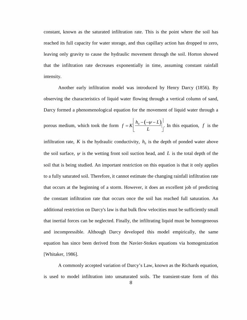
Another early infiltration model was introduced by Henry Darcy (1856). By

observing the characteristics of liquid water flowing through a vertical column of sand,

Darcy formed a phenomenological equation for the movement of liquid water through a

porous medium, which took the form f = Kh0 − −ψ − L( )

L

. In this equation, f is the

infiltration rate, K is the hydraulic conductivity, h0 is the depth of ponded water above

the soil surface, ψ is the wetting front soil suction head, and L is the total depth of the

soil that is being studied. An important restriction on this equation is that it only applies

to a fully saturated soil. Therefore, it cannot estimate the changing rainfall infiltration rate

that occurs at the beginning of a storm. However, it does an excellent job of predicting

the constant infiltration rate that occurs once the soil has reached full saturation. An

additional restriction on Darcy's law is that bulk flow velocities must be sufficiently small

that inertial forces can be neglected. Finally, the infiltrating liquid must be homogeneous

and incompressible. Although Darcy developed this model empirically, the same

equation has since been derived from the Navier-Stokes equations via homogenization

[Whitaker, 1986].

A commonly accepted variation of Darcy’s Law, known as the Richards equation,

is used to model infiltration into unsaturated soils. The transient-state form of this

9

equation is ∂θ∂t

=∂∂z

K θ( ) ∂ψ∂z

+1

, where K is the hydraulic conductivity as a function

of moisture content, ψ is the pressure head, z is the elevation, and θ is the moisture

content. The Richards equation is a non-linear partial differential equation, which is

therefore more difficult to solve than the linear Darcy’s Law. The Richards equation

states that the transfer of moisture through porous media over time is a function of

capillary suction, unsaturated hydraulic conductivity, and gravity.

Idealizations of the infiltration process are sometimes useful for characterizing the

primary mechanisms that underlie this phenomenon. One such idealization suggests that

the rainwater infiltrating into the soil can be characterized by an abrupt, propagating

wetting front, in which the soil below the wetting front is characterized by the initial

moisture content and the soil above the front is at complete saturation [Mein and Larson,

1971]. The speed at which the wetting front propagates is dependent on the rate of

rainfall (measured in depth of rain per time) and the hydraulic conductivity of the soil.

Three possible scenarios have been identified. Case A occurs when the rainfall rate is less

than the saturated hydraulic conductivity. In this case, the wetting front will infiltrate at a

constant rate equal to the rainfall rate, and the soil will never fully saturate. Case A

corresponds to curve 4 in Figure 1. Case B occurs when the rainfall rate is greater than

the saturated hydraulic conductivity, but less than the infiltration capacity. This stage

occurs at the beginning of a rainstorm, up until the point where the soil at the ground

surface reaches saturation, and the wetting front propagates at the same rate as the rainfall

intensity. Case B corresponds to the horizontal portions of curves 1, 2, and 3 in Figure 1.

The time for the ground soil moisture content to transition from the initial moisture

10

content to saturation (ts) depends on the intensity of the rainstorm. Case C occurs once

the soil at ground level has fully saturated and the rainfall intensity is greater than the

infiltration capacity. At this stage, runoff occurs on the surface since all of the rainwater

cannot infiltrate. Here, the wetting front propagation speed will decrease, and approach a

constant rate once the entire soil is saturated that will be a function of saturated hydraulic

conductivity and pressure head (as a result of puddling on the surface). Case C

corresponds to the decreasing portions of curves 1, 2, and 3 in Figure 1.

Figure 1. Infiltration curves for different rainfall intensities I1, I2, I3, and I4, where KS is the saturated hydraulic conductivity [Mein and Larson, 1971]. Alternatively, Mein and Larson (1971) divided the infiltration process into two

stages and developed finite difference models to obtain a numerical solution for each

stage. The first stage is similar to Case B above, and characterizes the conditions at the

very beginning of a moderate to severe rainstorm, when the rainfall intensity is higher

than the saturated hydraulic conductivity but lower than the initial unsaturated

11

conductivity. In this stage, all of the rainwater will completely infiltrate into the soil,

which is modeled as an abrupt wetting front perpetrating downward and governed by the

Richards equation. Since all of the water is infiltrating, it is logical that the infiltration

rate is equal to the rainfall rate, and thus the wetting front is assigned an initial downward

flow rate equal to the rainfall intensity. As more and more water enters the soil, the

potential gradient decreases and the infiltration capacity decreases until its value is equal

to the rainfall rate. The decrease in infiltration capacity allows the soil surface to

approach saturation. The second stage then occurs once the ground layer has reached full

saturation. Figure 2 shows the one-dimensional shape of the moisture field at the moment

of transition between these two stages. Here, the saturated soil has an infiltration rate

equal to the saturated hydraulic conductivity, which, in this case, is lower than the rainfall

rate. since in this case all of the rainwater cannot infiltrate, surface puddling and runoff

occur. In this model, the runoff is assumed to have negligible depth, and its influence on

infiltration rate due to head loss is thus ignored. At this point, Darcy’s Law is applied to

the wetting front, which maintains its shape but propagates deeper into the soil. Here the

infiltration rate is assigned a value equal to the saturated hydraulic conductivity of the

soil. Figure 3 demonstrates how the assumed wetting front moves downward at the rate

of saturated hydraulic conductivity.

12

Figure 2. A typical moisture content profile at the moment of surface saturation, where θi represents the initial moisture content and θs represents the saturated moisture content [Mein and Larson, 1971]

Figure 3. The assumed moisture content profile some time after the surface has saturated and the wetting front has propagated downward, where θi represents the initial moisture content and θs represents the saturated moisture content [Mein and Larson, 1971]

13

2.2 Heat Transfer Around Power Cables in Soil

The behavior of heat transfer through a porous medium, such as soil, is a well-

established field of physics. In this section, we focus on the specific problem of heat

transfer around buried power cables in the case where soil moisture is assumed to be

constant and independent from the soil temperature. Cases with variable soil moisture

content are discussed in the next section. A variety of different computational and

analytical models have been developed and implemented to solve for underground cable

temperature fields.

2.2.1 Thermal Conductivity

The mechanism of heat dissipation is a function of the physical properties of the

surrounding medium, of which the most important is the thermal conductivity [Anders

and Radhakrishna, 1988]. A common obstacle faced by many researchers was

determining an appropriate value for the thermal conductivity of the soil. Soil is almost

always a composition of several materials, such as stone, sand, silt, clay, air, and water,

all of which have different thermal characteristics. It was therefore necessary to develop a

model or equation to determine an effective thermal conductivity as a weighted average

of the conductivities of the individual soil components. There are many models that were

developed to obtain the thermal conductivity of soils, and there is disagreement amongst

researchers as to which method is most accurate.

Boguslaw and Lukasz (2006) present a comparison between six of the more

common experimental and numerical methods for determining soil conductivity, with

14

discussion of the benefits and limits of each. Among these different methods, two

approaches stand out and are discussed here. The first is a method originally proposed by

Kersten (1949), which determines the soil thermal conductivity experimentally by

measuring the temperature distribution resulting from a line heat source and then

comparing the resulting temperature field to the known analytical result. Since the

thermal properties are dependent on the soil composition, temperature, and moisture

content, the results of this method are only accurate for the specifically tested soil under

the given environmental conditions. The second method is known as the De Vries model

(1966), which is an analytical approach that takes a weighted average of the thermal

conductivities of each soil component (particles, water, and air) to determine the thermal

conductivity. This model was developed specifically for soil comprised of ellipsoidal

particles in a continuous media, and it includes parameters to account for the shape

factors of the particles and voids.

2.2.2 Analytic Methods

Early studies of underground cable heat transfer adopted an analytical approach

based on a lumped-parameter model of both the cable components and the soil. This

approach models the thermal transport as an electrical circuit, applying equivalents of

Ohm’s Law and Kirchhoff’s Law to the temperature field. Neher and McGrath (1957)

used this approach to model the temperature raise of a buried cable with both a steady

and a periodic heat load. The method also has the ability to account for multiple cables as

long as they are buried along the same vertical or horizontal axis. The governing equation

15

developed by Neher and McGrath has the form ∆Tc = Wc R i + qsR se + qe R ex + LF( )R xa( )[ ],

where Tc is the change of cable temperature, Wc is the losses developed in the cable

conductor, q is the ratio of losses in the sheath or conduit to the conductor, and the R’s

represent different resistances within portions of the thermal circuit. To solve the main

equation proposed by Neher and McGrath, the values of certain physical properties of the

soil and cable must be known, such as hydraulic conductivity and effective heat capacity.

Anders and El-Kady (1992) used the lumped-parameter approach to develop a transient

solution of the full thermal circuit of a buried cable. Their model included a correction

factor to account for the presence of a ductbank or backfill in which the cable in buried.

Backfill is a non-native material (often a mixture of sand, clay, and/or concrete) in which

the cable is buried as to take advantage of the backfill’s favorable thermal properties.

Their analytic method can also find a solution for a system of cables buried near each

other, and can even account for unequally loaded and dissimilar cables.

These lumped-parameter models are subject to a number of restrictions

which limit their usage. For instance, the models assume that the ground surface is

an isotherm, that cables are a line source of heat, and for transient calculations, that

the heat source changes as a series of discrete step functions. These models can be

used to obtain approximate solutions for buried cable heat transfer problems if the

cables are buried sufficiently deeply, that the different cables are well-separated

from each other, provided that the soil properties are homogeneous and that a

sufficient number of time step changes used to resolve the electrical load curve

[Anders, 1997; Aras et al., 2005].

16

2.2.3 Numerical Methods

Numerical solutions can be used to overcome the restrictions on the lumped

parameter approach discussed in the previous section. One common approach to this

problem is to employ a finite-element method for the temperature field in the soil around

the cable [Flatabo, 1973; Kellow, 1981; Nahman and Tanaskovic, 2003]. Kellow (1981)

solved for the heat dissipation from a distribution duct bank, in which a twenty duct

system contains sixteen cable-carrying ducts, two cooling ducts filled with water, and two

spare ducts. Situations with and without forced cooling within the duct were examined.

Nahman and Tanaskovic (2003) compared their finite element computational solution

with analytical approximations based on the lumped parameter approach. When

compared to experimental data, the finite element method results were in closest

agreement to the empirical data, which the authors claim to be due in part to the ability of

the numerical method to account for more complex boundary conditions, including solar

radiation and atmospheric convection.

Gela and Dai (1988) used a boundary element method to solve for the heat

migration in the vicinity of a buried power cable. The boundary element method has the

advantage of solving an integral equation over the domain boundaries, rather than a

differential equation in the interior region. This difference reduces a three-dimensional

computation into a two-dimensional problem, or in the case of a two-dimensional heat

transfer problem it reduces the two-dimensional computation to a one-dimensional

problem. However, when used to calculate the temperature field solution in a soil, certain

constraints arise. For instance, to model a multi-layered soil would require large amounts

17

of computational effort, since the soil interfaces would need to be considered as boundary

elements as well as the domain boundaries.

It is desirable that the solution domain size be large enough that the boundary

conditions do not significantly affect the temperature values near the cable. Therefore, the

size of the domain is typically very large compared to the cable diameter. Due to this

difference in length scale, a homogeneous grid that sufficiently resolves temperature near

the cable would require an enormous amount of calculations to solve for the whole

domain. A common approach to deal with this issue would be the use of a non-uniform

grid, with a progressively finer mesh near the cable. However, use of a Cartesian grid

simplifies the calculation and makes it possible for the researcher to achieve high

accuracy results with a finite difference approach, for instance using a centered difference

discretization. In such an approach, it is necessary to employ some type of overset grid

approach in order to introduce the cable into the Cartesian grid. Garrido et al. (2003) used

a finite difference approach to solve for the temperature field surrounding a cable system

in which they redistributed the heat flux from each cable onto a set of four grid cells

of the Cartesian grid. Overset grid methods involves a low-resolution Cartesian grid

throughout the domain and an overlaid, high-resolution polar grid in the vicinity of the

cable, with a numerical communication between the two grids. Vollaro et al. (2011) and

Marshall et al. (2013) used an outer Cartesian grid and an overlapping inner polar grid

surrounding each cable. Fringe points were identified on each grid, across which the

temperature field was interpolated at each time step. Both studies used a finite-difference

approach in both inner and outer grids, and Marshall et al. (2013) employed an ADI

18

formulation to accelerate calculations in the outer grid. Figure 4 shows the geometry and

location of the inner/outer grid communication.

Figure 4. Close-up figures showing (a) overlapping inner grid surrounding each cable and the outer Cartesian grid and (b) fringe points of the outer grid (open circles) and inner grid (filled circles). In (b), outer grid cells that overlap the outer boundary of the inner grid are shaded gray. [Marshall et al., 2013]

The effect of soil heterogeneity on cable heat transfer was examined by

Tarasiewicz et al. (1985). Hanna et al. (1993) also solved for heat transfer through multi-

layered soil, using a finite difference method. Kovač et al. (2006) examined the nonlinear

electric-thermal effects that arise due to temperature-dependent insulation electrical

resistance.

2.3 Coupled Heat and Moisture Transfer in Soil

The thermal conductivity of a soil is highly dependent on the moisture content,

and therefore the hydraulic properties of a soil are significant when making a complete

19

model of heat movement through soils. While the soil temperature field is dependent on

the soil moisture content field, the moisture content is also influenced by temperature

gradients, resulting in a coupled interaction between these two fields. The strong

dependence of the transport coefficients in these coupled equations (such as thermal

conductivity) on the temperature and moisture content values results in a strongly non-

linear problem.

2.3.1 Numerical Methods

Philip and De Vries (1957) present a coupled set of governing equations for heat

and moisture transfer in soils. Freitas and Prata (1996) developed a finite volume model

to solve the governing equations that were derived by Philip and De Vries for heat and

moisture transport in soil. They employed a Cartesian grid in which the cable is

represented by a heat source inside select grid cells. The coefficients representing soil

properties in the temperature and moisture content equations were obtained using a look-

up table, which interpolated between values obtained with two temperatures and 250

moisture content values. This numerical approach was used to examine the effect of

cyclic loading, progressive loading, and initial moisture content on the underground

cable’s conductor temperature. Figure 5 demonstrates the change in conductor

temperature over time, as a result of daily cyclic loading and progressive cyclic loading.

20

Figure 5. Variation of cable temperature for uniform and progressive cyclic load for a sandy silt soil with an initial moisture content value of 0.35 [Freitas and Prata, 1996] In a similar computational study, Anders and Rahakrishna (1988) solved Philip

and De Vries equations using a two-dimensional Galerkin finite element method. The use

of a finite element method allowed for more practical power cable configurations than the

finite difference method can accommodate. A key aspect of the moisture content field is a

migration of moisture away from the heated cable, resulting in a region surrounding each

cable with lower moisture content than for the ambient soil. The researchers were able to

validate their numerical model with an experimental field study, as can be seen in Figure

6.

21

Figure 6. Temperatures at surface of the outer cable for the directly buried cable experiments for measured data (dash-dot), heat/moisture program results (dashed), and heat only program results (solid) [Anders and Radhakrishna, 1988] Moya et al. (1999) solved the Phillips and De Vries equations using a finite

volume methodology for both steady and periodic heat fluctuations and initially

homogeneous moisture content. Their solutions led them to a conclusion that differs from

others presented thus far. Specifically, they claimed that, except for situations where a

large drying area occurs near the power cable, it is unnecessary to solve both the energy

and moisture transfer equations. Little difference was reported between the computed

solution of the heat conduction equation as compared to the solution to the coupled set of

equations for heat and moisture movement in soil. They determined that the most

significant influence of the moisture field on the temperature field is its affect on the

thermal conductivity of the soil, rather than the mechanism of directly transferring energy

via moisture migration. Therefore, in lieu of solving the coupled set of governing

22

equations, the researchers solved only the heat conduction equation with moisture-

dependent thermal conductivity.

All of the papers mentioned above assume uniform ambient moisture content with

no moisture added during the simulation. Since the time scales of the simulations are

large, in same cases spanning several months or even years, moisture addition via rainfall

would in reality be important in most situations. A recent study by Olsen et al. (2013)

predicts cable temperature fields in the presence of rainfall using a lumped-parameter

approach, in which change in soil moisture content is deduced by adjusting the soil

thermal conductivity and specific heat so that measured and predicted cable temperatures

will agree. The inclusion of precipitation in the model resulted in a direct cooling of the

cables that had not been considered by previous models.

2.3.2 Experimental Methods

Moya et al. (1999) present experimental results using a laboratory setup to model

heat transfer from a power cable buried in soil in the presence of uniform ambient

moisture at 30% moisture saturation. Using thermocouples to measure temperature and

tensiometers to determine moisture content, they presented results of the evolving

temperature field and moisture content in response to both constant and cyclic heating.

Unfortunately, the data from the tensiometers was reported by the researchers was

troublesome and not fully reliable.

Gouda et al. (2011) sought to experimentally determine the effect of a dry zone

around a buried cable in the presence of strong heating. Experiments were carried out for

23

6 types of natural soil by using thermocouples to determine the temperature of the soil at

different points radially outward from the central heat source. The readings from the

thermocouples were then plotted to create an approximate contour plot of the temperature

field. A sudden change of slope between thermocouple values, representative of a sharp

change in temperature gradient, insinuated that a dry zone had occurred, with the

interface of dry and wet soil located at the point where the slope changes. Using this data,

the researchers were able to approximate the temperature at which a certain soil would

begin drying. They solved the heat equation with fixed moisture content to solve for the

temperature field, and used the final temperature profile to estimate the final shape of the

dry zone. Since they never measured the soil moisture content, this paper instead

attempted to estimate the soil moisture indirectly by measuring the temperature field and

estimating the thermal conductivity of the soil. The study assumes that anywhere the soil

temperature was higher than a certain value, the soil was dry, and everywhere else the

soil is has some non-zero moisture value. The researchers tabulated data about each form

of soil and included the rate of formation of the dry zone.

24

CHAPTER 3: THEORY AND METHOD

3.1 Governing Equations

3.1.1 Coupled Heat and Moisture Transfer Equations

The governing equations for heat and moisture transfer within the ground are

given by the coupled system derived by Philip and de Vries (1957) as

)()( θλ θ ∇⋅∇+∇⋅∇=∇⋅+∂∂

Vw DLTTCt

TC v , (3.1)

y

KDTD

t T ∂

∂+∇⋅∇+∇⋅∇=

∂∂ θ

θ θθ

)()( , (3.2)

where ),( tT x is the temperature field and ),( txθ is the volumetric moisture content. The

various coefficients in (3.1)-(3.2) include the volumetric heat capacity of wet soil C, the

volumetric heat capacity of water Cw, the water velocity vector v , the unsaturated

hydraulic conductivity θK , the soil thermal conductivity λ , the latent heat of

vaporization of water L, the thermal moisture diffusivity TD , the isothermal moisture

diffusivity θD , and the isothermal vapor diffusivity VDθ . Equation (3.1) is derived from

Fourier’s Law and the conservation of energy, with modifications to include the thermal

migration effect of moisture gradients as well as the convective forces of bulk water flow.

In equation (3.1), the second term on the left-hand side represents thermal convection by

the liquid motion, and on the right-hand side, the first term represents thermal diffusion,

25

and the second term represents energy transfer via latent heat of the vapor caused by a

moisture gradient.

Equation (3.2) is derived from a combination of the continuity equation and

Richard’s Equation, an extension of Darcy's law to unsaturated media. Additionally, a

modified form of Fick’s Law, derived by Penman (1939), is incorporated into Richard’s

Equation to account for vapor transfer. The continuity equation gives an expression for

the rate of change of the moisture content as

0=⋅∇+∂∂

Qt

θ, (3.3)

where Q is the net water flux (defined to be positive upward), which is equal to the

product of the water velocity v and the soil porosity η . An equation for Q was derived by

Philip and de Vries (1957) in terms of the temperature and moisture gradients as

)(/ yT KDTD evQ θθ θη +∇+∇−== , (3.4)

where the first and second terms on the right-hand side are associated with transport of

water by capillary action and the third term is associated with gravitational transport.

Substituting this expression into the continuity equation (3.3) gives the moisture balance

equation (3.2). Equations (3.1)-(3.2) are the same equations used by previous

investigators for cable ampacity computation [Anders and Radhakrishna, 1988; Freitas et

al., 1996; Moya et al., 1999], with the important difference that the thermal convection

26

term is also included in order to properly account for the effect of rainfall on the

temperature field.

3.1.2 Coefficient Definitions

The coefficients λ , TD , θD , L, C, VDθ , and θK are functions of the temperature

and moisture content. Since analytical expressions for these coefficients are difficult to

obtain, it is common practice to evaluate them using empirical formulas developed for

specific soil types. In the current study, a representative backfill soil was selected, which

is identified as Soil III by Anders and Radhakrishna (1988). This soil is described as

well-graded with course to fine particles, such as is found in a silty sand or a sandy loam.

It has a porosity of 0.45 which in the range of typical values for this type of soil. The

equations used for the coefficients for this soil type are given by Anders and

Radhakrishna (1988) as

dryedrysat K λλλλ ++= )( ,

TVTLT DDD += , VL DDD θθθ += , (3.5)

lvwhL ρ= , θρρ wwSs ccC +=

where 1log += SKe , satS θθ /≡ , and the various coefficients in (3.5) are given in Table

1. The empirical equation for effective thermal conductivity in (3.5) is restricted to

1.0≥S . When 1.0<S , the soil is nearly dry, so we set dryλλ = in the computations. A

27

plot of the thermal conductivity as a function of moisture content is given in Figure 7.

There is a slope discontinuity in this plot at 045.0=θ , but this discontinuity does not

influence the computational results since the moisture content in the computations is

always greater than this value.

Figure 7. Plot of the effective thermal conductivity of soil used in the computations as a function of moisture content.

28

Table 1. Expressions used for the variable coefficients that characterize heat and moisture transport in the soil as functions of temperature T (in degrees Kelvin) and relative moisture content satS θθ /≡ . The different coefficients are in SI units, as indicated in the

nomenclature section.

Variable Parameters Constant Parameters

TLD = )96.2601.8exp( −S 45.0=satθ

TVD = )316.23416.1exp( −− S 3.0=dryλ

LDθ = )19.1806.8exp( −S 6.1=satλ

VDθ = )792.27483.7exp( −− S 1800=sρ

lvh = T)00237.0(10496.2 6 −× − 1000=wρ

θK = 6610 S− 1480=Sc

4216=wc

3.2 Computational Method

3.2.1 Assumptions and Limitations

Certain simplifications and restrictions had to be imposed on the problem so that

it complied with the requirements and limitations of the chosen governing equations and

numerical method. It was assumed that a two-dimensional cross-section of the soil-cable

domain would yield sufficient information about the complete three-dimensional system,

as there would be symmetry along the axis of the cable. For the governing equations to be

relevant, the moisture field throughout the soil must maintain continuity. To satisfy this

29

constraint for a soil with non-zero initial moisture content value, there cannot be any

zones where complete drying occurs. Therefore, the moisture content was numerically

restricted to a minimum value greater than zero. Additionally, the soil surface was not

allowed to fully saturate, as this would cause an instability in the numerical method and

yield unrealistic results. The instability occurs because in areas where the soil is fully

saturated, the diffusion terms in the governing equations approach small values.

Simultaneously, the propagation of the saturated wetting front causes a large convection

value. When the convection term is dominant over diffusion, the chosen numerical

method is unstable. Consequently, it was assumed that if the surface was to approach

saturation due to heavy rain, all of the excess rainwater would become runoff and could

be neglected, and the surface would remain just below saturation. A more complete

model may account for a puddling effect, caused by a rain intensity that is higher than the

soil infiltration capacity, which would create an additional pressure head term on the top

boundary due to the layer of ponded water on the soil surface. But for this model, the

simulated rainfall intensities were restricted to values that would not fully saturate the

soil surface. Fortunately, the soil characteristics and rainfall data chosen for the

production runs of this simulation never lead to a saturated surface or a complete dry-out

zone anyway. Therefore, the two aforementioned limitations did not actually affect the

final computational results. Finally, it was assumed that any presence of a water table

beneath the bottom boundary could be neglected, as the domain depth was sufficiently

shallow. Thus there was never any addition of water from the bottom boundary.

30

3.2.2 Computational Domain and Boundary Conditions

The numerical computations are performed on both an outer Cartesian grid and on

an inner polar grid surrounding a single buried cable, as shown in Figure 8. The outer

grid has boundaries at x = ±1

2Hx in the horizontal direction, and it extends from the

ground to a depth y = −Hy . The four boundaries of the outer grid are identified by circled

numbers [1] - [4] in Figure 8. On the bottom boundary [4], the temperature is set to a

prescribed value 0T and the moisture content is governed by a flux balance of the form

θθ

θK

yD

y

TDT −=

∂∂

+∂∂

. (3.6)

Zero-flux boundary conditions are used for temperature on the side boundaries [2] and

[3], so that 0/ =∂∂ xT . The side boundary condition for moisture is again based on the

flux balance, and is given by

0=∂∂

+∂∂

xD

x

TDT

θθ . (3.7)

A convective boundary condition for temperature is used on the top boundary [1], which

has the form

0)( =∂∂

+−+∂∂

yLDTTh

y

TVatm

θλ θ , (3.8)

31

where h is the surface heat transfer coefficient and atmT is the atmospheric temperature.

The third term is included along with the tradition convective boundary equation to

account for the transfer of latent heat by vapor migration. The boundary condition for

moisture content on the top boundary [1] is

rainT QKy

Dy

TD =+

∂∂

+∂∂

θθ

θ, (3.9)

where )(tQrain denotes the prescribed time-varying flux of water supply by rain on the

top boundary.

Figure 8. Schematic diagram of the computational flow domain and the inner (polar) and outer (Cartesian) grids, where the cable is identified as a black circle at the center of the inner grid, which is submerged a depth b below the ground. The boundaries of the outer grid are identified by circled numbers.

32

3.2.3 Overset Grids

The outer Cartesian grid computations are performed by introducing a heat source

for grid cells of the outer grid that overlap the cable cross-section. The heat supply rate to

each outer grid cell, outf , is related to the cable surface heat flux inq by

outgcin fANRq =π2 , (3.10)

where R is the cable radius, cN is the number of outer grid cells that receive a heat

supply, and gA is the area of one cell of the outer grid.

The outer grid yields an accurate solution for heat and moisture transport in the

region sufficiently far away from the cable, but it does not satisfy the boundary

conditions on the cable surface. In order to obtain a more accurate solution near the cable,

we use an overset inner grid in an annular region spanning from the cable radius R to the

outer radius IR of the inner grid. The center of the inner grid is located a distance b

below the ground level, where b is called the cable burial depth. Within this inner grid,

the temperature and moisture content fields are discretized using a polar coordinate

system ),( φr . The inner grid solution satisfies the flux boundary condition in temperature

and the no-penetration condition for moisture on the cable surface, so that

inqr

T=

∂∂

− λ , 0=∂∂

r

θ on Rr = . (3.11)

33

The two grids communicate on the set of grid points on the outer boundary of the inner

grid ( IRr = ), which are called fringe points. At each time step, we first solve for the

temperature and moisture fields on the outer grid, and then use a bilinear interpolation to

set the values of T and θ at the fringe points of the inner grid, denoted by fT and fθ .

The inner solution is then solved using a Dirichlet boundary condition on its outer surface

of the form

fTT = , fθθ = on IRr = . (3.12)

3.2.4 Numerical Method

The governing equations (3.1)-(3.2) for temperature and moisture content were

solved within both the inner and outer grids using a Crank-Nicholson method for the

diffusive terms and a second-order Adams-Bashforth method for the convective term,

with the velocity given by (3.4). Spatial derivatives were computed using second-order

centered differences in both grids. The resulting system of equations was solved using a

Gauss-Seidel iteration method, which was written such that computations are performed

only with non-zero matrix elements. It is noted that (3.1) approaches a first-order

hyperbolic equation in the absence of the diffusive terms, for which the numerical

method described above would not be stable. This numerical instability was not an issue

for most scenarios in the current computations, however, since the scale of the problem is

fairly small (ranging from centimeters to tens of meters) and the diffusive terms were

consequently sufficiently large to suppress the instability. However, it did cause

34

instabilities when the soil fully saturated, as discussed in the restrictions subsection

above. The CFL number xtv ∆∆ /max was monitored for all computations and did not

exceed 0.002.

3.2.5 Dimensionless Parameters

The problem depends upon two dominant length scales - the cable diameter d and

the cable submergence depth b. The cable diameter characterizes small-scale fluctuations

of temperature and moisture around the cable, such as are associated with power load

fluctuations during a daily cycle, but the submergence depth is more characteristic of the

thermal and moisture fields as a whole.

Three characteristic time scales in the problem are referred to as the convective

time scale Cτ , the diffusive time scale Dτ , and the load-variation time scale Lτ . If we

select b as a characteristic length scale, the convective time 0/ θτ KbC = is the typical

time required for a rain front to propagate from the ground to the cable location, where

0θK is characteristic of the velocity scale caused by gravitational drainage. The diffusive

time 02

0 / λτ bCD = , where 00 / Cλ is a characteristic thermal diffusivity, is representative

of the time required for the thermal field to attain a steady state upon change of the cable

heat flux or of the surrounding moisture field. The load-variation time Lτ represents the

period of oscillation of the cable heat load, where we make the common assumption that

the cable load is periodic on a daily cycle. For typical conditions, Cτ is on the order of 11

days, Dτ is on the order of 20 days, and Lτ is 1 day. The addition of rain at the top

35

boundary introduces other time scales which can be compared to the three time scales

described above. These additional scales include the rain duration time Rτ and the period

between rain events Pτ , both of which are examined in the paper.

A set of dimensionless variables are defined using the cable submergence depth b

as a length scale, the load-variation time Lτ as the time scale, the average cable surface

heat flux q , and the ambient temperature 0T . The resulting dimensionless variables

(denoted with primes) are defined by

)( 00 TTbq

T −=′λ

, ∇=∇′ b , Ldttd τ/=′ , bxx /=′ , byy /=′ ,

0/ θKvv =′ , outout fq

bf =′ , qqq inin /=′ , 0/ θKQQ rainrain =′ ,

0/ CCC =′ 0/ λλλ =′ 0/ LLL =′ 0/ VVV DDD =′ ,

0/ TTT DDD =′ , 0/ θθθ DDD =′ , 0/ θθθ KKK =′ . (3.13)

A subscript “0” is used to denote constant nominal values of the coefficients, where these

nominal values are set equal to the coefficient values under saturated soil conditions

(obtained from (3.5) and Table 1 with 1=S ).

The dimensionless governing equations and boundary conditions contain a

number of different dimensionless parameters. In the current paper, we hold many of

these dimensionless parameters constant in order to focus on a small number of

parameters that characterize the rainfall. Characteristic values of these dimensionless

36

parameters are obtained for a typical 5kV distribution cable (e.g., a tape-shielded 5kV 4/0

AWG aluminum conductor), for which the average cable diameter is 5.2=d cm, the

burial depth is 1=b m, and a typical cable surface heat flux is q = 500 W/m2 for an

average-size residential community (Marshall et al., 2013). Using a typical value for

thermal conductivity of fully saturated soil of W/mK6.10 =λ , we obtain a relationship

between a change in the dimensionless temperature T ′∆ and the dimensional temperature

T∆ as TCT ′∆°=∆ )5.312( . A list of constant dimensionless parameters and the values

used for these parameters in the current computations is given in Table 2. The

dimensionless parameters that are allowed to vary in the computations include the rainfall

intensity, the rainfall duration parameter LRrainD ττ /= , and the dimensionless rainfall

frequency Lff τ=′ .

37

Table 2. List of dimensionless parameters whose values are held fixed, and their values in the current computations.

Parameter Name Equation Typical Value

convH 0λ

hb

2.8

c1 2

0

0

bCLλτ

5.2 210−×

c2

71cc

1.2 1010−×

c3 b

Dq TL

0

0

λτ

0.16

c4 2

0

b

DL θτ

3.5

c5

τL Kθ 0

b

8.6 210−×

c6

05 C

cc wwρ

0.14

c7 bq

DL V 00

2.4 910−×

c8 bqD

D

T 0

00 θλ

22

m1

00

0

θλ K

Dq T

1.9

m2 bK

D

0

0

θ

θ

40

3.2.6 Grid Independence and Validation

A grid independence study was performed to examine sensitivity of the

computations to number of grid points in the inner and outer grids. Since the focus of the

study is on effect of soil characteristics and rain on the thermal and moisture exposure of

38

a buried cable, the grid independence study examines the effect of grid resolution on the

average temperature and moisture content on the cable surface as a function of time. The

test computation used for the grid independence study was conducted for a case where

the initial temperature field is set equal to the ambient temperature ( 0)0,( =′ xT ) and the

initial moisture content was 1.0),( =yxθ . The domain size was Hx /b = 5.0 and

Hy /b = 3.0, with a cable diameter d /b = 0.0249 and an inner grid radius RI /b = 0.0747.

The depth of the bottom boundary is selected to be sufficiently deep so as not to

significantly influence the moisture and temperature fields around the cable, but at the

same time sufficiently shallow that it might reasonably be assumed to be above the water

table. The cable surface heat flux was held constant ( 1=′surfq ) and the rain flux was set at

5.0=′rainQ . The time step was fixed as 002.0=′∆t , and the runs were continued out to

20=′t . The number of grid points in the inner grid was set such that the grid spacing at

the outer edge of the inner grid in both the radial and azimuthal directions was similar to

the grid spacing used in the outer grid. In the grid independence study, the number of

points in the inner and outer grids were varied in the same proportion. Three different

grids were examined in the study, with grid point numbers in each direction in the inner

and outer grids listed in Table 3. Results for the average cable surface temperature and

moisture content are plotted in Figure 9 as functions of time for each grid. For the finest

two meshes, the maximum difference in cable surface temperature was 0.5% and the

maximum difference in moisture content was 1.1%. The computations in the remainder

of the paper were performed on the medium-resolution mesh B.

39

(a) (b) Figure 9. Time variation of the average cable surface temperature and moisture content for the grid independence study, for grids A (dash-dot), B (solid), and C (dashed).

The sensitivity of the temperature field to the thermal convection term was

examined by repeating the computation described above with grid B but with no thermal

convection term. The prediction for the average dimensionless temperature on the cable

surface is compared with the result with the thermal convection term in Figure 10. It is

observed that the results are similar for the runs with and without convection during the

initial part of the calculation as the cable temperature increases before the rain front

penetrates to the cable location. At about 4=′t , the cable temperature abruptly begins

decreasing, coinciding with the abrupt increase in moisture content observed in Figure 9b

associated with arrival of the moisture front from the rainfall event at the cable location.

Following this time, the predictions with and without the convection term in Figure 10

exhibit significant differences. The most noticeable of these differences is that the cable

temperature prediction without convection rapidly asymptotes to a constant value

40

following arrival of the moisture front, whereas the cable temperature prediction with

convection exhibits a gradual decrease with time.

Figure 10. Comparison of predicted dimensionless average cable surface temperature for a case with the thermal convection term (solid line) and without the thermal convection term (dashed line) for the same run as shown in Figure 9.

The rate of rainwater infiltration demonstrated longer time scales than the

researchers originally expected, and therefore it was important to compare this result with

previous research to ensure accuracy. The rainwater infiltration behavior in this

simulation was validated by comparing it to the solutions of a commercial rainfall

infiltration modeling software, known as CHEMFLO-2000. The software only models

one-dimensional water infiltration, so the current model was simplified by removing the

cable and inner grid, setting the temperature field equal to zero, and resetting all thermal

boundary conditions to a temperature equal to zero. After the simulation was run, a

41

vertical slice of data was taken from the domain, allowing for a relevant one-dimensional

comparison with the control software solution. For the comparison to be useful, the initial

conditions and soil characteristics of the current model were set as closely as possible to

those conditions used in the specific CHEMFLO-2000 simulation that was used for

validation here. That requirement meant using an initial condition of 0.08 uniform

moisture content, and a top boundary condition of a 0.8 dimensionless rainfall intensity

for 12 hours. The one-dimensional moisture content data from this simulation was plotted

for every 2 hours, and compared with the results from the control simulation, as seen in

Figure 11. One difference that may be noticed is that the shapes of the curves nearer the

surface of the soil differ between the two models, especially as time progresses. At higher

time values, the curves of the CHEMFLO-2000 results have more horizontal slopes than

the results from the current model. This is because the commercial software uses a

saturated moisture content of 0.31, while the current model uses a value of 0.45. As the

soil surface reaches saturation in the commercial model, the moisture gradient value

asymptotes towards zero, as can be seen in the figure. As mentioned above in the

limitations subsection, the current code yielded inaccurate results when the surface was

allowed to fully saturate. Therefore, due to this restriction in the current model, it was not

possible to perfectly recreate the CHEMFLO-2000 simulation. Instead the saturated value

was kept at 0.45, and thus a sharp gradient of moisture content value remains near the

surface. Despite this difference in comparing the two results, it can also be seen that the

general shape of the curves are similar and that the effect of the rainfall on the moisture

content is felt at similar depths within the soil at a given point in time, insinuating that the

42

rate of infiltration is similar for both simulations. Therefore, although the software model

does not agree well with the current model’s solution for water content near the soil

surface, it agrees very well at greater depths under the surface. Since the cable, which is

the focus of the study, is buried at a depth in which the rainfall infiltration models agree

well, the comparison can be said to validate the accuracy of the current model.

(a) (b)

Figure 11: Comparison of the one-dimensional moisture content value over a 12 hour rainstorm of intensity 0.8 between (a) the current model and (b) the CHEMFLO-2000 commercial software

43

CHAPTER 4: RESULTS AND DISCUSSION

Computational results are reported in this section for thermal and moisture fields

around underground cables with periodic rainfall events. The rainfall intensity, duration,

and period are all varied in such a way that the average rainfall is held constant, and the

results are compared to computations with constant average rainfall in order to determine

the transient effects caused by rainfall events.

4.1 Initialization

4.1.1 Finding the Steady State Moisture Field

The computations are initialized using two sets of preliminary computations. The

first preliminary computation is performed with the outer grid only for constant rainfall

and with no cable present. Since this problem is essentially one-dimensional, the outer

grid is reduced to 637 points in the y-direction and 11 points in the x-direction for the first

preliminary computation. The constant rainfall rate is determined by dividing the average

annual precipitation in different regions by the number of days in a year, and then non-

dimensionalized to obtain rainQ ′ , where the overbar denotes average value. Computations

were performed with 005.0=′rainQ , 0.01, 0.02, and 0.03, as well as the case with no rain

( 0=′rainQ ). The case with 03.0=′rainQ corresponds to a precipitation of 95 cm/yr, which

is typical of Chicago, whereas that with 01.0=′rainQ corresponds to a precipitation of 32

cm/yr, which is typical of Los Angeles. For simplicity, rainfall is spread throughout the

year and seasonal variations are ignored. Each computation is initialized using a uniform

44

moisture content of 1.00 =θ and temperature set equal to the ambient value. The

computations are continued until a steady-state condition is achieved in the value of

moisture content to at least four significant figures. The case with no rain did not achieve

a steady-state value even after very long time, but instead decreased very slowly with

time in a continuous manner. The steady-state moisture profiles for the four cases with

non-zero values of rainQ ′ are plotted as functions of the dimensionless depth by /−≡ξ in

Figure 12. The line denoted by 'E' in this figure shows the moisture content profile for the

case with no rain at a time approximately 10 years after the initial condition.

Figure 12. Steady-state moisture content profiles for cases with (A) 03.0=′rainQ , (B)

0.02, (C) 0.01, (D) 0.005, and (E) 0 as a function of dimensionless depth ξ . The initial moisture profile in the calculations is indicated by a dashed line. For the case with no rain, the moisture content moves downward very slowly in time and no steady-state profile is observed. The moisture profile shown in E is plotted at a time of approximately 10 years after the initial condition. The other cases have all converged to steady-state profiles within four significant figures in the moisture content.

45

4.1.2 Finding the Steady State of Coupled Temperature and Moisture Field

The second preliminary computation reads in the equilibrium moisture content

profile for the selected average rainfall rate, and then introduces the cable with a constant

surface heat flux using both the outer and inner grids with the number of grid points set

equal to the values stated for grid B in Table 3. In the second preliminary computation,

the rainfall rate is held constant at the same average value as used for the first

computation. The computations are continued until both the temperature and moisture

content fields have achieved steady-state values. The time variation of the average

temperature and moisture content on the cable surface are plotted in Figure 13 as

functions of time for the four cases with non-zero rainfall shown in Figure 12, showing

the approach of the results to a steady-state condition. In Figure 13a, the dimensionless

temperature is shown on the left-hand y-axis and the corresponding change in

dimensional temperature (in C° ) for the example problem with 2 W/m500=q , m 1=b ,

and W/mK6.10 =λ is shown on the right-hand y-axis.

Table 3. Number of points in different grids used in grid independence study. Grid Identification Outer Grid Inner Grid

x y r φ

A 651 451 37 63

B 921 637 53 89

C 1029 711 59 99

46

(a) (b) Figure 13. Time variation of the average cable surface (a) temperature and (b) moisture content during the second preliminary computation for cases with (A) 03.0=′rainQ , (B)

0.02, (C) 0.01, and (D) 0.005. In (a), the dimensionless temperature is shown on the left-hand y-axis and the corresponding change in dimensional temperature for the example problem is shown on the right-hand y-axis. The figure shows the approach of the temperature and moisture content fields to a steady state condition. The contours of the steady-state temperature and moisture content around the

cable are plotted for the case with 03.0=′rainQ in Figure 14. In this figure, the near-cable

inner grid is superimposed on the outer grid so that the fields are accurately represented

both near to and far away from the cable. Contours of the temperature and moisture

content fields are observed in close-up images to vary smoothly and continuously across

the two grids. Also, the value of temperature and moisture content is extracted on the

vertical line 0=x , passing through the cable, and plotted in Figure 15 for the four

different rainfall rates in their steady-state solutions. As expected, the temperature field

exhibits a local maximum at the cable and decays away from the cable. From Figure 15,

we observe that the temperature peak value does not differ significantly between the four

47

different rainfall rates examined, although the temperature falls off more rapidly with

distance away from the cable for the higher rainfall rate case, as is consistent with the

higher thermal conductivity caused by higher values of moisture content. The moisture

content exhibits a local minimum near the cable for all four rainfall rates, which

corresponds to a region in which the moisture content contour lines are locally raised

upward as they pass over the cable. This effect also persists for some distance below the

cable. The presence of rainfall causes the region of decreased moisture fraction (i.e., the

'dry' region) surrounding the cable to become asymmetric, with a sharper moisture

gradient above the cable than below the cable.

48

Figure 14. Steady-state (a) dimensionless temperature and (b) moisture content fields at the end of the second preliminary computation for the case with 03.0=′rainQ .

(a)

(b)

49

(a) (b) Figure 15. Variation of (a) temperature and (b) moisture content on the line 0=′x as a function of dimensionless depth ξ for the same four values of rainQ ′ shown in Figure 6. In

(a), the dimensionless temperature is shown on the left-hand y-axis and the corresponding change in dimensional temperature for the example problem is shown on the right-hand y-axis.

4.2 Periodic Variation in Rainfall Intensity, Duration, and Frequency

The result of the second preliminary computation is used as an initial condition

for a series of computations examining the effect of rainfall transients on cable thermal

and moisture exposure. In each of these computations, the rainfall is assumed to occur

periodically in time, with intensity, duration, and frequency that are consistent with the

specified average rainfall rate in the preliminary computations. Each set of computations

is compared with the result of the steady-state computation with constant rainfall rate.

The focus is specifically on two regions, one fairly moist (typical of Chicago, Illinois)

and one fairly dry (typical of Los Angeles, California). The average dimensionless

rainfall rates for these two regions are approximately 03.0≅′rainQ and 0.01,

50

corresponding to 940 and 325 mm/yr, respectively. According to Sun et al. (2006), 67%

of the precipitation occurs in 15 days in Los Angeles and in 30 days in Chicago, yielding

a dimensionless frequency of Lff τ≡′ of 0.04 and 0.08, respectively. Rainfall intensity

varies from about 2.5 mm/hr for a light rainfall to between 10-50 mm/hr for a heavy

rainfall, with a characteristic value of 10 mm/hr for a moderate rainfall. When non-

dimensionalized using 60 10−=θK m/s, the characteristic value of the instantaneous

dimensionless rainfall intensity, rainQ′ , is approximately 2.5. Dividing the total annual

precipitation by the characteristic rainfall intensity (10 mm/hr) times the number of rainy

days gives a typical rainfall duration of about 2.5 hours, or 1.024/5.2 ≅=rainD . Using

these characteristic values, a listing of computational runs was formulated as shown in

Table 4. The first runs D1 and M1 are based on the characteristic conditions, runs D2-D3

and M2-M3 vary intensity and duration with fixed frequency, runs D4-D5 and M4-M5

vary duration and frequency with fixed intensity, and runs D6-D7 and M6-M7 vary

intensity and frequency with fixed duration.

Results are shown in Figures 16-18 for Run D1, characteristic of a dry climate

(e.g., Los Angeles). The average cable surface temperature and moisture content are

plotted in Figure 16 as functions of time. The computation is performed over a time

interval of 600 days, during which 24 rainfall periods occur. Even though the

computation is initialized at the steady-state condition for the same value of average

rainfall rate as used in the D1 computation, it is observed that the temperature and

moisture fields approach a periodic limit-cycle state in which the mean temperature and

moisture content on the cable surface has very different values than in the steady-state

51

condition. The approach of the system from the steady-state solution to a limit-cycle state

is shown in Figure 17, which plots the dimensionless cable surface temperature as a

function of the cable surface moisture content. In this limit-cycle condition, the mean

cable surface dimensionless temperature decreases by about 0.008 and the mean moisture

content increases by about 0.04 compared to the steady-state solution. The oscillation

amplitude of the dimensionless cable surface temperature in the limit-cycle state is

0003.0≅′ampT and the amplitude of the moisture content on the cable surface is

0044.0≅ampθ .

The drift between the steady-state solutions and the averaged values of the limit-

cycle solutions is necessarily a behavior caused by the nonlinearity within the system.

The mechanisms that are responsible for the nonlinearity include the bulk flow

convection term and the complex dependence of the various soil coefficients (thermal

conductivity, etc.) on the temperature and moisture content. A series of computations

were performed to determine the specific nonlinear agent responsible for the drift

behavior. One of these computations repeated case D1 but omitted the convection term,

and another computation held the different soil coefficients at constant values. The results

of the first computation showed little difference in the solution between the cases with

and without the convection term. However, when the soil coefficients values were held

constant, the averaged values of the limit-cycle condition solution was approximately

equal to the steady-state solution, as would be expected in a linear system. These

computations clarify that the complex dependence of the various soil coefficients on the

soil temperature and the moisture content are responsible for the nonlinear drift of the

52

average temperature and moisture content fields in the periodic rainfall case relative to

the steady state case.

A more physical explanation of this nonlinear drift behavior can be accredited to

the inherently hysteretic response of soil to infiltrating moisture. The hysteretic effect

occurs because hydraulic conductivity of soil increases in value as the local moisture

content value increases. In other words, water will infiltrate into a moist soil more

quickly than a drier soil. With this concept applied to the current study, it can be

understood that a more intense rainfall event will result in a stronger demonstration of

this hysteresis. Compared to the low-intensity rainfall experienced during the preliminary

steady-state runs, the simulated rainstorms in the production runs cause a dramatic spike

of moisture content value at the surface of the soil. As the rainstorm continues, this

increased moisture content allows for the incoming rainfall to infiltrate more quickly, as a

result of the higher local hydraulic conductivity. The more intense penetration of

rainwater causes a more dramatic change in local temperature and moisture content

value. Therefore, the drift seen in the results from the steady-state to the limit-cycle

condition is a product of the soil hydraulic conductivity hysteresis.

53

Table 4. Listing of rainfall conditions used for periodic rainfall computations in conditions typical of dry and moist climates. Rainfall is characterized by the dimensionless rainfall intensity 0/ θKQQ rainrain =′ , duration LRrainD ττ /= , and frequency

Lff τ=′ . The computational results are listed for the change in the mean values of

dimensionless temperature and moisture content from the steady-state solutions, surfT ′∆

and surfθ∆ , and the oscillation amplitude of the dimensionless temperature and moisture

content in the periodic solution, ampT ′ and ampθ .

Dry Climate ( 01.0=′rainQ )

Rainfall Characteristics Computational Results Run Intensity Duration Freq.

surfT ′∆ ampT ′

surfθ∆ ampθ

D1 2.5 0.10 0.04 - 0.0081 0.00031 0.040 0.0044 D2 1.0 0.25 0.04 - 0.0076 0.00029 0.037 0.0041 D3 5.0 0.05 0.04 - 0.0097 0.00039 0.040 0.0052 D4 2.5 0.20 0.02 - 0.0085 0.00093 0.042 0.0115 D5 2.5 0.05 0.08 - 0.0074 0.00009 0.037 0.0015 D6 5.0 0.10 0.02 - 0.0104 0.00130 0.045 0.0146 D7 1.25 0.10 0.08 - 0.0067 0.00008 0.033 0.0013

Moist Climate ( 03.0=′rainQ )

Rainfall Characteristics Computational Results

Run Intensity Duration Freq.

surfT ′∆ ampT ′ surfθ∆ ampθ

M1 2.5 0.15 0.08 - 0.0094 0.00038 0.050 0.0060 M2 1.0 0.375 0.08 - 0.0088 0.00036 0.047 0.0058 M3 5.0 0.075 0.08 - 0.0082 0.00043 0.044 0.0069 M4 2.5 0.30 0.04 - 0.0101 0.00111 0.056 0.0145 M5 2.5 0.075 0.16 -0.0077 0.00012 0.042 0.0020 M6 5.0 0.15 0.04 -0.0088 0.00127 0.048 0.0170 M7 1.25 0.15 0.16 -0.0073 0.00011 0.040 0.0021

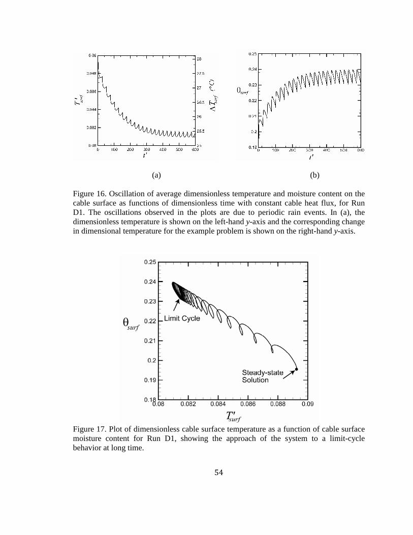
54

(a) (b) Figure 16. Oscillation of average dimensionless temperature and moisture content on the cable surface as functions of dimensionless time with constant cable heat flux, for Run D1. The oscillations observed in the plots are due to periodic rain events. In (a), the dimensionless temperature is shown on the left-hand y-axis and the corresponding change in dimensional temperature for the example problem is shown on the right-hand y-axis.

Figure 17. Plot of dimensionless cable surface temperature as a function of cable surface moisture content for Run D1, showing the approach of the system to a limit-cycle behavior at long time.

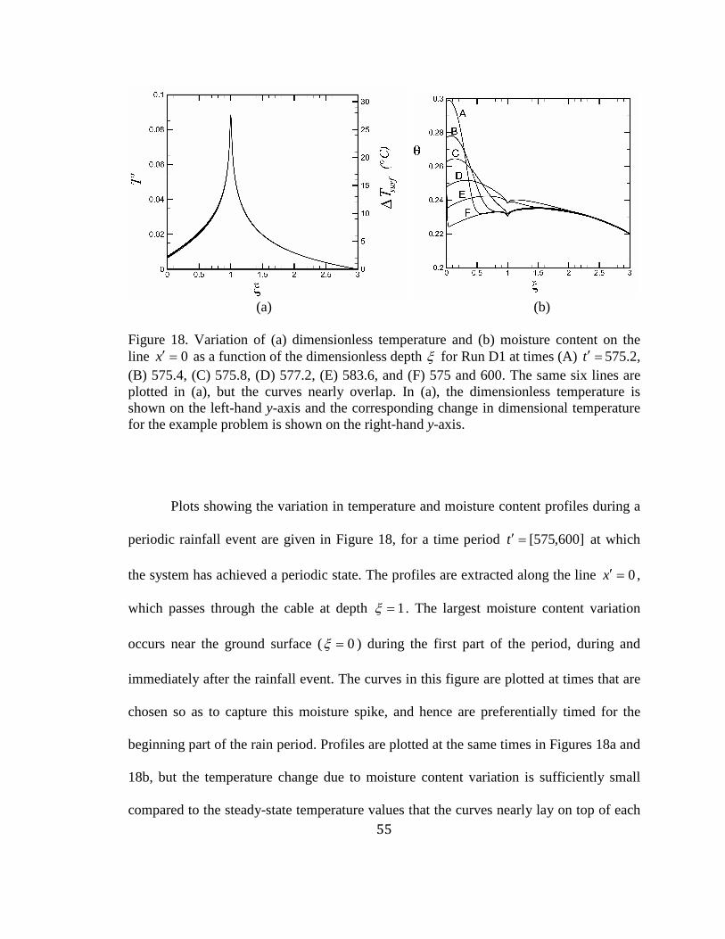
55

(a) (b)

Figure 18. Variation of (a) dimensionless temperature and (b) moisture content on the line 0=′x as a function of the dimensionless depth ξ for Run D1 at times (A) =′t 575.2, (B) 575.4, (C) 575.8, (D) 577.2, (E) 583.6, and (F) 575 and 600. The same six lines are plotted in (a), but the curves nearly overlap. In (a), the dimensionless temperature is shown on the left-hand y-axis and the corresponding change in dimensional temperature for the example problem is shown on the right-hand y-axis. Plots showing the variation in temperature and moisture content profiles during a

periodic rainfall event are given in Figure 18, for a time period ]600,575[=′t at which

the system has achieved a periodic state. The profiles are extracted along the line 0=′x ,

which passes through the cable at depth 1=ξ . The largest moisture content variation

occurs near the ground surface ( 0=ξ ) during the first part of the period, during and

immediately after the rainfall event. The curves in this figure are plotted at times that are

chosen so as to capture this moisture spike, and hence are preferentially timed for the

beginning part of the rain period. Profiles are plotted at the same times in Figures 18a and

18b, but the temperature change due to moisture content variation is sufficiently small

compared to the steady-state temperature values that the curves nearly lay on top of each

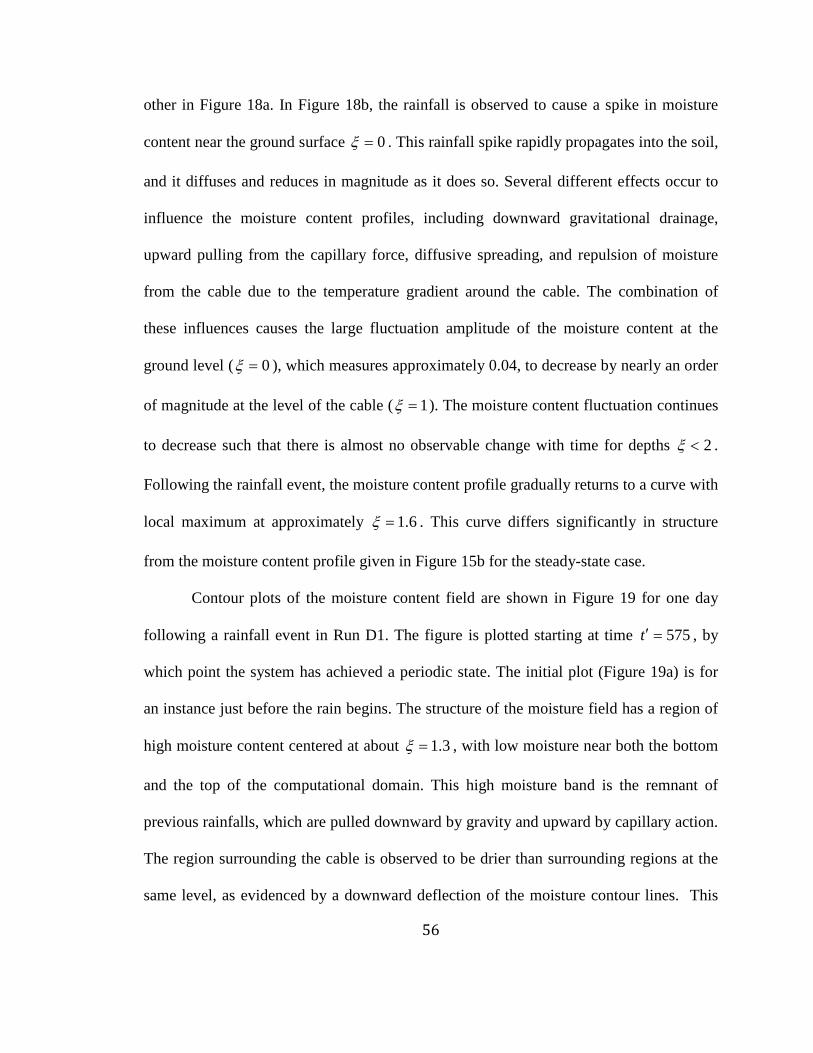
56

other in Figure 18a. In Figure 18b, the rainfall is observed to cause a spike in moisture

content near the ground surface 0=ξ . This rainfall spike rapidly propagates into the soil,

and it diffuses and reduces in magnitude as it does so. Several different effects occur to

influence the moisture content profiles, including downward gravitational drainage,

upward pulling from the capillary force, diffusive spreading, and repulsion of moisture

from the cable due to the temperature gradient around the cable. The combination of

these influences causes the large fluctuation amplitude of the moisture content at the

ground level ( 0=ξ ), which measures approximately 0.04, to decrease by nearly an order

of magnitude at the level of the cable ( 1=ξ ). The moisture content fluctuation continues

to decrease such that there is almost no observable change with time for depths 2<ξ .

Following the rainfall event, the moisture content profile gradually returns to a curve with

local maximum at approximately 6.1=ξ . This curve differs significantly in structure

from the moisture content profile given in Figure 15b for the steady-state case.

Contour plots of the moisture content field are shown in Figure 19 for one day

following a rainfall event in Run D1. The figure is plotted starting at time 575=′t , by

which point the system has achieved a periodic state. The initial plot (Figure 19a) is for

an instance just before the rain begins. The structure of the moisture field has a region of

high moisture content centered at about 3.1=ξ , with low moisture near both the bottom

and the top of the computational domain. This high moisture band is the remnant of

previous rainfalls, which are pulled downward by gravity and upward by capillary action.

The region surrounding the cable is observed to be drier than surrounding regions at the

same level, as evidenced by a downward deflection of the moisture contour lines. This

57

structure differs significantly from that shown in Figure 7b for the steady-state

simulation. At time 2.575=′t (Figure 19b), the rain event has recently ended and a

region with high moisture content is observed at the top of the figure. This region of high

moisture content propagates downward with time in Figures 19c-f, eventually overtaking

the dry region around the cable. Over longer time, the high-moisture region from the

previous rainfall will move downward and merge into the high-moisture region located

just below the cable, so that by the end of the period at 600=′t , the moisture field looks

the same as shown in Figure 19a.

Results are presented in Figures 20 and 21 for Run M1, characteristic of a

moderately moist climate (e.g, Chicago). The trends in the data are qualitatively the same

as was observed under drier conditions in Figures 16 and 18. The cable surface

temperature and moisture content transition from the steady-state solution to approach a

limit-cycle state. The mean dimensionless cable surface temperature decreases by about

0.0094 and the mean cable surface moisture content increases by about 0.050 in this

limit-cycle state compared to the values in the steady-state solution. The fluctuations in

dimensionless surface temperature and moisture content during each rainfall cycle occur

with amplitude 0004.0≅′ampT and 006.0≅ampθ , which are slightly larger than the values

observed for Run D1. The temperature profile in Figure 21a is not significantly affected

by the moisture variation, but the moisture profile in Figure 21b exhibits a large spike

near the upper surface during and immediately after the rainfall event, with the moisture

content increasing by approximately 0.1 at 0=ξ during each rainfall cycle. As was the

case with Run D1, the fluctuation in moisture content decays rapidly with depth,

58

decreasing by about an order of magnitude by the level of the cable. The moisture content

is observed to settle in the later part of each period to the same hump-type profile as

noted in Figure 18b for Run D1, for which the moisture content is a maximum at an

intermediate depth.

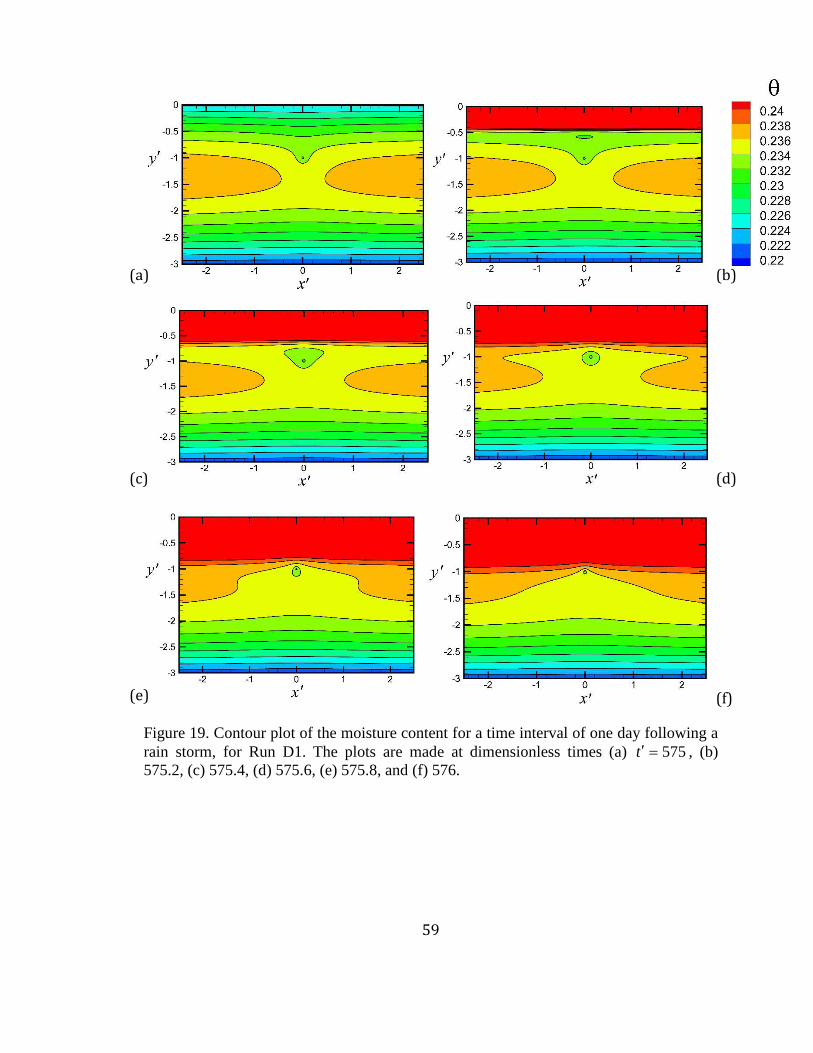
59

Figure 19. Contour plot of the moisture content for a time interval of one day following a rain storm, for Run D1. The plots are made at dimensionless times (a) 575=′t , (b) 575.2, (c) 575.4, (d) 575.6, (e) 575.8, and (f) 576.

(a) (b)

(c) (d)

(e) (f)

60

(a) (b) Figure 20. Oscillation of average dimensionless temperature and moisture content on the cable surface as functions of dimensionless time with constant cable heat flux, for Run M1. The oscillations observed in the plots are due to periodic rain events. In (a), the dimensionless temperature is shown on the left-hand y-axis and the corresponding change in dimensional temperature for the example problem is shown on the right-hand y-axis.

(a) (b) Figure 21. Variation of (a) dimensionless temperature and (b) moisture content on the line 0=′x as a function of the dimensionless depth ξ for Run M1 at times (A)

=′t 587.6, (B) 587.8, (C) 588.0, (D) 588.4, and (E) 590.0, and (F) 587.5 and 600. The same six lines are plotted in (a), but they nearly overlap. In (a), the dimensionless temperature is shown on the left-hand y-axis and the corresponding change in dimensional temperature for the example problem is shown on the right-hand y-axis.

61

The system response for Runs D2-D7 and M2-M7 were qualitatively similar to

that described above for Runs D1 and M1. In all cases with periodic rainfall, the cable

surface temperature and moisture content approach a periodic limit-cycle condition in

which the mean cable surface temperature decreases and the mean cable surface moisture

content increases compared to the steady-state solutions. A listing of the change in

dimensionless cable surface temperature and moisture content and the amplitude of

oscillation of these values in the limit-cycle state is given in Table 4 for Runs D1-D7 and

M1-M7. The results in this table exhibit a strong dependence of the oscillation amplitude

on the rain frequency, but a weaker dependence on rainfall intensity and duration

(provided the total rainfall amount is fixed).

Figure 22 plots the computed oscillation amplitude for the dimensionless cable

surface temperature and the cable moisture content as functions of dimensionless

frequency f ′ for all of the conditions examined. The oscillation amplitude values for the

moist conditions (Runs M1-M7) are substantially greater than for the dry conditions

(Runs D1-D7). The amplitudes for the cable surface temperature and moisture content

decrease as the rainfall frequency increases. Since the total annual rainfall amount for the

dry and moist conditions is fixed, higher frequency cases correspond to conditions with

frequent rainfall events containing small amounts of precipitation, whereas low frequency

cases correspond to conditions with infrequent rainfall events that contain large amounts

of precipitation. It is noted that the oscillation amplitude is rather small for both the cable

surface temperature and the moisture content. For instance, for the example problem with

burial depth 1=b m and average cable heat flux q = 500 W/m2, the largest oscillation

62

amplitude values for the cable surface temperature and moisture content in the

computations conducted were C°4.0 and 0.017, respectively. By comparison, the

temperature field obtained by Marshall et al. (2013) for the same example case oscillated

due to the daily power load variation with amplitude of C°9.3 , or an order of magnitude

larger than the rain-related oscillation amplitude.

Plots are shown in Figure 23 for the difference between the dimensionless cable

surface temperature and the cable surface moisture content in the periodic limit-cycle

condition and the initial values for the steady-state case, denoted by meanT ′∆ and meanθ∆ .

The dimensionless cable surface temperature decreases with periodic rainfall by an

amount between 0.006 and 0.011, where the magnitude of the temperature change

decreases with increase in the rainfall frequency. The cable surface moisture content

increases with periodic rainfall by an amount ranging between 0.033 and 0.056, where

the change in moisture content also decreases with increase in rainfall frequency. Again

using our example problem with 1=b m and q = 500 W/m2, the change in mean cable

surface temperature under the periodic rainfall condition corresponds to a decrease of

C°− 5.30.2 .

63

(a) (b) Figure 22. Amplitude of average cable surface (a) dimensionless temperature and (b) moisture content fluctuations with periodic rain events as functions of dimensionless rain frequency. Results are for the moist condition (triangles, dashed line) and the dry condition (circles, solid line) listed in Table 4. The curves are exponential fits to the data. In (a), the dimensionless temperature is shown on the left-hand y-axis and the corresponding change in dimensional temperature for the example problem is shown on the right-hand y-axis.

(a) (b) Figure 23. Change in mean values of the average cable surface (a) dimensionless temperature and (b) moisture content with periodic rain events as functions of dimensionless rain frequency. Results are for the moist condition (triangles, dashed line) and the dry condition (circles, solid line) listed in Table 4. The curves are exponential fits to the data. In (a), the dimensionless temperature is shown on the left-hand y-axis and the corresponding change in dimensional temperature for the example problem is shown on the right-hand y-axis.

64

CHAPTER 5: CONCLUSIONS AND FUTURE WORK

5.1 Conclusions

A study of the effect of periodic rainfall events on the surface temperature and

moisture exposure of a buried electric cable was conducted using numerical simulations.

Cases with different rainfall intensity, duration, and frequency were compared to a

steady-state case with the same annual precipitation amount. Computations were

conducted for two values of the annual precipitation, one typical of a relatively moist

climate and one typical of a dry climate. In the steady-state condition, the computations

indicate formation of a relatively dry region surrounding the cable in which the moisture

content decreases by about 2-5% compared to the value that it would have had without

the cable present. Under periodic rainfall conditions, the cable surface temperature and

moisture content transition to a limit-cycle behavior with values that oscillate periodically

in time with the rainfall frequency. Of particular interest is the observation that the mean

values of the cable surface temperature and moisture content in this limit-cycle condition

are significantly different from the steady-state values, with the mean cable surface

temperature decreasing and the moisture content increasing in value under the limit-cycle

condition relative to the steady-state condition. Both the oscillation amplitudes and the

change in mean values relative to the steady-state condition are observed to depend

primarily on the rainfall frequency and on the annual precipitation amount, such that the

absolute values of these quantities decrease as the rainfall frequency or the annual

precipitation amount increase. While the computed values of the oscillation amplitude of

65

the cable surface temperature are rather small, measuring C°4.0 or less in the current

computations, the change in the mean cable surface temperature between the steady-state

and limit-cycle conditions is found to be large, measuring as high as C°5.3 in the current

computations. Similarly, the largest computed value of the oscillation amplitude of the

moisture content (0.017) is small compared to the largest computed value of the change

in mean cable surface moisture content between the limit-cycle and steady-state

conditions (0.056). It was demonstrated that the drift in the mean temperature and

moisture content values between the steady-state and limit-cycle conditions is a result of

the nonlinear dependence of the various soil coefficients on the temperature and moisture

content. Despite both conditions resulting from an equivalent amount of annual

precipitation, the limit-cycle condition demonstrates lower cable temperatures because

the rainfall events occur in short but intense periods, relative to the steady-state

simulation. The higher intensity rainfall causes a more intense penetration of the soil

wetting front, which results in strong, nonlinear changes in the transport coefficients.

The results of the current study have shown that periodic rainfall conditions result

in fundamentally different moisture and temperature fields around an underground cable

compared to what would be observed under steady-state rainfall conditions. Not only do

the moisture content and temperature values oscillate periodically in time when exposed

to periodic rainfall events, but the time-averaged values of the moisture content and

temperature also change significantly in this periodic case compared to their steady-state

values. The change in the mean values causes decreased values of the cable surface

temperature, but increased values of the cable surface moisture content. As a

66

consequence, steady-state computations which do not include intermittent rainfall events

over-estimate the temperature-related degradation of the cable insulation but under-

estimate the moisture-related insulation degradation.

5.2 Applications and Future Work

The knowledge gained from this research can help improve the efficiency of

underground power delivery and increase the lifespan of the buried power cables. Power

companies can utilize a method similar to that described here to simulate the local soil

state under different weather conditions, and then develop local power delivery standards

based on the results. By contrast, the current system of national standards may over- or

under-restrict the amount of electricity that can be efficiently and safely transported by

the cable in any given location. The results of this study demonstrate that rainfall events

have a significant effect on the thermal and moisture content fields surrounding a buried

power cable, and that ampacity limits should account specifically for the frequency of

rainfall in a given area.

For future work, certain additions could be made to the existing computational

model to improve its accuracy and overall usefulness. It would be very helpful for

simulating a greater variety of possible rainstorm types if the soil surface was allowed to

saturate fully. This would require the use of a numerical method that retained good

numerical stability when convection becomes the dominant transport mechanism.

Similarly, if a fully saturated condition were allowed the method could be used for

problems with a shallow water table, in which the water table was included in the

67

computational domain. In many regions, the water table is shallower than three meters, as

is assumed in the current work. It would also be helpful if the computational method

could account for a complete dry-out zone. Though total drying did not occur in the

current solutions, its occurrence may be more relevant in areas with desert-like climates.

It would be useful if the model had the ability to simulate the behavior of heat

and moisture migration for different types of soils, so that the simulation is more easily

adaptable to different geographical areas. While the current numerical method readily

accommodates different soil types, it would be necessary to develop a data bank that

contains relevant information and coefficients for different soils. Such a data bank would

also allow us to simulate problems where the power cable is buried in a backfill material

surrounded by the native soil, as well as other problems where soil heterogeneity is

prominent.

Other improvements could be made by using real-world data for certain source

values, rather than imposing a simplified representation of those systems. For instance,

one could model varying cable loads based on real-world data. Likewise, it would be very

useful to model the rainfall events in a way that more closely replicates real-world

rainfall data. It was shown in this paper that the results differed significantly when

comparing a steady rainfall scenario to a periodically varying rainfall scenario. Therefore,

it is fair to suggest that it would be necessary to model the rainfall events with

stochastically varying intensity, duration, and frequency, as such events occur in reality,

to determine the most accurate results for the thermal and moisture content fields around

a buried cable.

68

REFERENCES

G.J. Anders, Rating of Electric Power Cables. Ampacity Computations for Transmission,

Distribution, and Industrial Applications, IEEE Press, New York, 1997.

G. J. Anders and M. A. El-Kady, “Transient ratings of buried power cables. Part 1.

Historical perspective and mathematical model,” IEEE Trans Power Delivery, vol.

7(4), pp. 1724-1734, 1992.

G. J. Anders, H. S. Radhakrishna, “Computation of temperature field and moisture

content in the vicinity of current carrying underground power cables,” IEE

Proceedings, vol. 135(1), pp. 51-61, 1988.

F. Aras, C. Oysu, G. Yilmaz, “An assessment of the methods for calculating ampacity of

underground power cables”, Electric Power Components Systems, vol. 33(12), pp.

1385-1402, 2005.

J. Y. Baladi, D. L. Ayers, and R. J. Schoenhals, “Transient heat and mass transfer in

soils,” Journal of Heat and Mass Transfer, vol. 24, pp. 449-458, 1981.

U. Boguslaw and U. Lukasz, “Thermal conductivity of soils—Comparison of

experimental results and estimation methods,” Institute of Agrophysics, 2006.

E. Buckingham, "Studies on the Movement of Soil Moisture”, US Department of

Agriculture, Bureau of Soils, Bulletin No. 38, pp. 61, 1907.

E. C. Childs, “An introduction to the physical basis of soil water phenomena,” J. Wiley

and Sons Ltd., pp. 493, 1969.

H. Darcy, “Les Fontaines Publiques de la Ville de Dijon,” Dalmont, Paris, 1856.

69

M. Deru, “A model for ground-coupled heat and moisture transfer from buildings,”

Doctoral Dissertation, Colorado State University, 2003.

D. A. De Vries, “Thermal Properties of Soils.” Physics of Plant Environment, North-

Holland Publishing Company, 1966.

D. A. De Vries and N. H. Afgan, “Heat and mass transfer in the biosphere”, John Wiley

and Sons, 1975.

N. E. Edlefsen and A. B. C. Anderson, “Thermodynamics of soil moisture,” Hilgardia,

vol. 15(2), pp. 31-298, 1943.

M. J. Eppstein, D. K. Grover, J. S. Marshall, and D. M. Rizzo, “An agent-based model to

study market penetration of plug-in hybrid electric vehicles,” Energy Policy, vol. 39,

pp. 3789-3802, 2011.

O. T. Farouki, “Thermal Properties of Soils,” CRREL Monograph 81-1, U.S. Army

Cold Regions Research and Engineering Laboratory, New Hampshire, 1981.

L. P. Fernández, T. G. San Román, R. Cossent, C. M. Domingo, and P. Frías,

“Assessment of the impact of plug-in electric vehicles on distribution networks,”

IEEE Trans. Power Systems, vol. 26(1), pp. 206-213, 2011.

N. Flatabo, “Transient heat conduction problems in power cables solved by finite element

method,” IEEE Trans Power Apparatus Systems, vol. 92(1), pp. 56-63, 1973.

D. S. Freitas, A. T. Prata, “Thermal performance of underground power cables with

constant and cyclic currents in presence of moisture migration in the surrounding

soil,” IEEE Trans. Power Delivery, vol. 11(3), 1996.

70

O. Fuhrer, “Inverse heat conduction in soils: A new approach towards recovering soil

moisture from temperature records,” Doctoral Dissertation, ETH Zurich, 2000.

C. Garrido, A. F. Otero, and J. Cidras, “Theoretical model to calculate steady state and

transient ampacity and temperature in buried cables,” IEEE Trans Power Delivery,

vol. 18(3), pp. 667-678, 2003.

G. Gela, J. J. Dai, “Calculation of thermal fields of underground cables using the

boundary element method,” IEEE Trans Power Delivery, vol. 3(4), pp. 1341-1347,

1988.

M. T. van Genuchten, “A Closed-Form Equation for Predicting the Hydraulic

Conductivity of Unsaturated Soils.” Soil Science Society American Journal, Vol. 44;

pp. 892–898, 1980.

O. E. Gouda, A. Z. El Dein, and G. M. Amer, “Effect of the formation of the dry zone

around underground power cables on their ratings,” IEEE Trans. on Power Delivery,

vol. 26(2), pp. 972-978, 2011.

M. A. Hanna, A. Y. Chikhani, and M. M. A. Salama, “Thermal analysis of power cables

in multi-layered soil. Part 1. Theoretical model,” IEEE Trans Power Delivery, vol.

8(3), pp. 761-771, 1993.

D. Hillel, Environmental Soil Physics. San Diego, CA: Academic Press, 1998.

O. Johansen, “Thermal conductivity of soils,” Institute for Kjoleteknikk, 1975.

M.A. Kellow, “A numerical procedure for the calculation of the temperature rise and

ampacity of underground cables,” IEEE Trans Power Apparatus Sys, vol. 100(7), pp.

3322-3330, 1981.

71

M. S. Kersten, “Thermal properties of soil”, Bulletin of the University of Minnesota,

Institute of Technology, vol. 52, pp. 1–225, 1949.

N. Kovac, I. Sarajcev, and D. Poljak, “Nonlinear-coupled electric-thermal modeling of

underground cable systems,” IEEE Trans Power Delivery, vol. 21(1), pp. 4-14, 2006.

O. Krischer and H. Rohnalter, “Warmeleitung und dampfdiffusion in feuchten gutern,”

Verein Deut. Ing.-Forschungsheft, vol. 402, 1940.

J. Marshall, P. Hines, J. Zhang, F. Minervini, and S. Rinjitham, “Modeling the impact of electric vehicle charging on transient heat transfer around underground cables,” Electric Power Systems Research, vol. 97, pp. 76-83, 2013.

R. Mein and C. L. Larson, “Modeling the infiltration component of the rainwater-runoff

process,” Masters Dissertation, University of Minnesota, 1971.

E. E. Miller and R.D. Miller, “Physical Theory for Capillary Flow Phenomena,”

Journal of Applied Physics, Vol. 27; pp. 324–332, 1956.

R. E. S. Moya, A. T. Prata, and J. A. B. Cunha Neto, “Experimental analysis of unsteady

heat and moisture transfer around a heated cylinder buried into a porous medium,”

Journal of Heat and Mass Transfer, Vol. 42, pp. 2187-2198, 1999.

M. Muskat, “The Flow of Homogeneous Fluids Through Porous Media”, McGraw-Hill

Book Company, Inc., New York, pp. 763, 1937.

N. Nakano and T. Miyazaki, “The diffusion and nonequilibrium thermodynamic

equations of water vapor in soils under temperature gradients,” Soil Science, Vol.

128(3), pp. 184-188, 1979.

72

J. Nahman, M. Tanaskovic, “Calculation of the ampacity of medium voltage self-

supporting cable bunch,” Electric Power Systems Research, vol. 93, pp. 106-112,

2003.

J. H. Neher and M. H. McGrath, “The calculation of the temperature rise and load

capability of cable systems,” AIEE Trans, Part 3, vol. 752-763, pp. 752-763, 1957.

R. Olsen, G.J. Anders, J. Holboell, and U.S. Gudmundsdottir, “Modelling of Dynamic

Transmission Cable Temperature Considering Soil-Specific Heat, Thermal

Resistivity, and Precipitation”, IEEE Transactions on Power Delivery, vol. 28(3), pp.

1909-1917, 2013.

H. L. Penman, “Gas and vapour movement in soil,” Journal of Agricultural Science, vol.

30, pp. 437-466, 1939.

J. R. Philip and D. A. De Vries, “Moisture movement in porous materials under

temperature gradients,” Trans. American Geophysical Union, vol. 38(2), pp. 222-232,

1957.

L. A. Richards, “Capillary Conduction of Liquids Through Porous Mediums," Physics,

Vol. 1, pp. 318-333, 1931.

E. Tarasiewicz, E. Kuffel, and S. Grybowsji, “Calculation of temperature distributions

within cable trench backfill and the surrounding soil”, IEEE Trans. Power Apparatus

Systems, vol. 104(8), pp. 1973-1978, 1985.

L. R. Vollaro, J. Fontana, and A. Vallati, “Thermal analysis of underground electric

power cables buried in non-homogeneous soils,” Applied Thermal Engineering, vol.

31, pp. 772-778, 2011.

73

S. Whitaker, “Flow in porous media I: A theoretical derivation of Darcy’s Law,”

Transport in Porous Media, vol. 1, pp. 3-25, 1986.

effect of rainfall events on the thermal and moisture

Documents