i

THESIS FOR THE DEGREE OF DOCTOR OF PHILOSOPHY

Efficiency of building related pump and fan operation

Application and system solutions

CAROLINE MARKUSSON

Building Services Engineering Department of Energy and Environment

CHALMERS UNIVERSITY OF TECHNOLOGY Göteborg, Sweden 2011

ii

EFFICIENCY OF BUILDING RELATED PUMP AND FAN OPERATION Application and system solutions Caroline Markusson © CAROLINE MARKUSSON, 2011 ISBN 978-91-7385-588-4 Doktorsavhandling vid Chalmers tekniska högskola Ny serie nr 3269 ISSN 0346-718X Technical report D2011:02 Building Services Engineering Department of Energy and Environment Chalmers University of Technology SE-412 96 GÖTEBORG Sweden Telephone +46 (0)31 772 1000 Printed by Chalmers Reproservice Göteborg 2011

iii

Efficiency of building related pump and fan operation Application and system solutions CAROLINE MARKUSSON Building Services Engineering Chalmers University of Technology

Abstract The electric energy use in Swedish non-industrial buildings is 71 TWh per year out of which 30 TWh per year is used for the operation of technical systems. A significant part of those 30 TWh/year is used for pump and fan operation. The Swedish parliament decided in 2009 on a national energy and climate plan. By the year 2050 the energy use per unit conditioned floor area in the Swedish building stock must be halved compared to the year of 1995. The objective of this thesis is to find means to reduce pump and fan energy in the non-industrial buildings. The aim is to find systems and components that can provide energy reduction in pump and fan systems by 50 %. In the thesis the current situation in non-industrial buildings regarding pump and fan systems has been described and the energy saving potentials, both at component and at system level, have been identified and discussed. Furthermore, the possibility of decentralized pump and fan systems has been examined. The calculated saving potential is 50 % and 40 % respectively for pump and fan operation in non-industrial buildings. This may be achieved by improving pump efficiency and specific fan power to state-of-the-art efficiency and recommended SFP values. System changes can also provide major additional energy savings in pump and fan operation. A decentralized pump heating system has been implemented in real life and results show a reduction of pump energy by 70 %. The theoretical parts of the thesis are supported by four case studies in real buildings and by three laboratory studies. Keywords: air systems, control-on-demand, decentralized systems, efficiency,

electric energy, electric motor, fan, hydronic systems, local systems, motor drive, pump, variable speed,

iv

This thesis has been funded by the Swedish Energy Agency/CERBOF (project no. 430547-1), Formas-Bic (project no. 244-2008-99) and Göteborg Energi foundation for Research and Development (project no. 10-2008-0165/13) within the project Energy efficient pump and fan operation in buildings to Building Services Engineering of Chalmers University of Technology.

v

Acknowledgment The financial support given by Göteborg energy, Energimyndigheten and Formas Bic is gratefully acknowledged. In addition I would like to thank all the companies that have been involved in the project for their times spent and valuable discussions. Special thanks to Honeywell, Wilo, Grundfos, LGG Inneklimat, LogiCO2, Swegon, Akademiska hus and Västfastigheter for helping me with test objects and equipment. I would like to thank my supervisor Ass. Professor Lennart Jagemar for his guidance, encouragement and shared knowledge. I would like to thank Professor Per Fahlén for giving me this opportunity and for sharing his knowledge and visions. I would also like to thank all my colleagues at Building services engineering. Especially thanks to Håkan Larsson for his invaluable help and patience in the laboratory and Tommy Sundström for all his help and support with measurements and computers. Finally, I would like to thank Prof. Torbjörn Thiringer and Dr. Johan Åström at the Division of Electric Power Engineering for good cooperation. My love is reserved for my family who has always been there for me. Companies involved in the project:

Akademiska hus LogiCO2 Astra Zeneca Mare Trade Cadcom MedicHus Göteborgs Stads Bostads Nibe Danfoss Swegon Fläkt Woods Systemair Gothia Power Schneider Electric Grundfos Thermia Värme Göteborg Energi Tour and Andersson Honeywell Västfastigheter IVT Wilo LGG Inneklimat Åf –Installation

Göteborg October 2011 Caroline Markusson

vi

vii

Contents Page Abstract iii Acknowledgment v

Symbols x 

Latin letters x Greek letters x Subscripts xi 

Abbreviations xii Dimensionless numbers xii 

1  Introduction 1 1.1  Background 1 1.2  Objective 1 1.3  Methodology 1 1.4  Outline of the thesis 2 1.5  List of publications 2 2  Literature review 5 2.1  Pumps and liquid systems 5 2.2  Fans and air systems 9 2.3  Electric motors and motor drives 13 2.4  Literature review summary 15 3  Building related electric energy to pumps and fans in Sweden 17 3.1  Energy use and conditioned floor area for non-industrial buildings 17 3.2  Pump operation – power, time of operation and energy use 20 3.3  Fan operation – power, time of operation and energy use 27 3.4  Pump and fan energy use - summary 33 4  Current HVAC system design - Pump and fan duty 35 4.1  Design criteria 35 4.2  Liquid systems 37 4.3  Air systems 39 4.4  Current use and future possibilities 41 5  Future HVAC system design - Pump and fan duty 43 5.1  Design criteria 43 5.2  Liquid systems 44 5.3  Air systems 46 5.4  Requirements on future components and control systems 49 5.5  Discussion 61 6  System simulation example 63 6.1  Model and model validation 63 6.2  Simulation for case study II 70 7  Case studies and laboratory tests 77 7.1  Case study I: Conventional use of central VSD pumps 77 7.2  Case study II: Future design with local VSD pumps/ centralized to decentralized pump system design 84 7.3  Case study III: Heat exchangers - run around loop and enthalpy wheel 92 7.4  Case study IV: Air heaters and air coolers 103 7.5  Laboratory test I: Pump efficiency 108 

viii

7.6  Laboratory test II: Control of heating-coil capacity by local VSD pump 114 7.7  Laboratory test III: Control of cooling-coil capacity by local VSD pump 116 8  Discussion, conclusions and future work 123 8.1  Discussion 123 8.2  Conclusion 125 8.3  Future work 127 References 129 Appendix A 137 

Flow measurements 137 Budget of uncertainty for the flow measurement 139 Differential pressure measurements 139 Power measurements 140 Uncertainty budget for the pump efficiency measurement 140 

ix

x

Symbols

Latin letters C heat capacity flow rate ( C M c p ) [W/K]

cp specific heat capacity at constant pressure (fluids) [J/(kg·K)] D diameter [m] n rotational speed [revs/s] p pressure (pressure difference is designated p, see ) [Pa] Q thermal capacity [W]

SFP Specific Fan Power [kW/(m3/s)] SPP Specific Pump Power [kW/(m3/s)] T torque [Nm] t celsius temperature [°C] U thermal transmittance (total coefficient of heat transfer) [W/(m2K)] V volume [m3] V volume flow rate [m3/s] W power (mechanical or electric) [W]

tW technical power (mechanical or electric) [W]

K radiator constant [W/Kn] n radiator exponent [-]

Greek letters

valve authority [-] p pressure difference [Pa or kPa] lm logarithmic mean temperature difference [K or °C] am arithmetic mean temperature difference [K or °C] ε effectiveness [-] efficiency [-] t temperature efficiency [-] density [kg/m3] time [s] angular velocity [radians/s]

xi

Subscripts

Medium A air B brine w l

water liquid

Component

Cv control valve

Bv balancing valveHu heating unit

F fan

P pump

Position

1 inlet

2 outlet

R room

xii

Abbreviations AHU Air Handling Unit BLDC Brushless Direct Current CA Cooling Agent (pump) CC Condenser Coolant (pump) CAV Constant Air Volume COP Coefficient Of Performance DC Direct Current DCV Demand Control Ventilation EC Electronically Commutated ECR Energy Cost Ratio EEI Energy Efficiency Index EF Exhaust Fan (only) HA Heating Agent pump HR Heat Recovery (pump) HVAC Heating, Ventilation, Air-Conditioning HW Service Hot Water HWC Hot Water Circulation IM Induction Motor NTU Number of Transfer Units NV Natural Ventilation OA Other Applications SEF Supply and Exhaust Fan VAV Variable Air Volume VSD Variable Speed Drive PER Primary Energy Ratio PM Permanent Magnet PWM Pulse Width Modulation

Dimensionless numbers

NTU Number of Transfer Units; NTUU A

C

U A

M cp

( )min min

1

1 Introduction The electric energy use in Swedish non-residential building is 71 TWh per year of which 30 TWh per year is used for the technical operation. A significant part of those 30 TWh is used for pump and fan operation. The Swedish parliament decided in 2009 on a national energy and climate plan. Year 2050 the energy use in the Swedish building stock must be halved compared to the year of 1995. An intermediate target is to reduce the energy use by 20 % by year 2020. To be able to meet this target for pump and fan systems new system solutions and better component efficiencies is necessary.

1.1 Background Pumps are used in many applications in buildings such as hydronic heating and cooling systems. The individual pump power is small; however there is a great quantity of pumps in buildings. Often pumps have long operational hours and poor efficiency and as a consequence the energy use by pumps is significant. The control of heating/cooling capacity in hydronic systems is achieved by the use of control valves. The control valve direct and quantity the flow rate in the system, however, the control valve also constitutes a significant pressure drop in the system. Heating and cooling loads varies in a buildings and the design situation (heating, cooling, air flow, etc.) is needed only a fraction of the total operational time. Nevertheless, pumping power is usually constant and independent of heating or cooling need. Fans are used in building mechanical ventilation systems. In many cases the fan is situated in an air handling unit in line with air-heater, air-cooler, filter and heat exchanger. Many of the components in an AHU are operated at reduced load or at no load at all during part of the operational time but are still causing a pressure drop in the AHU. Further, occupancy in buildings is varying and in many cases low. Thus, there is a potential for energy saving by using demand control pump and fans systems and reducing system pressure drops. Frequency converters and more efficient motors have recent years become available for smaller applications such as pumps and fans. This opens up for alternative system solutions using direct flow control by variable speed drive pumps and fans.

1.2 Objective The objective of this thesis is to find means to reduce pump and fan energy in non-industrial buildings. The aim is to find systems and components that can provide energy reduction in pump and fan systems by 50 % according to the Swedish national target.

1.3 Methodology To achieve the objectives the following activities have been undertaken:

- The current situation in non-industrial buildings regarding pump and fan systems has been described

- Energy saving potentials both on component and on system level has been indentified and discussed

- The possibility of decentralized pump and fan systems has been examined

2

For the two first chapters literature review is the main instrument. Available literature and statistics have been examined and summarized. Also a survey of available pumps and fans on the market has been conducted. For all the case studies, field measurements have been conducted and theory and modelling in Matlab has been used for the analysis of the investigated systems. Laboratory measurements have been conducted to investigate component performance and for model validation.

1.4 Outline of the thesis Chapter 1 is the introduction part of this thesis, where the background, objective and scope and methodology are given. In Chapter 2 a literature review is presented. The literature review accounts for pump systems, fans systems, electric motors and motor drives. The review of pump and fan systems can be divided into three parts; control, system design and fan/pump efficiency. Chapter 3 gives a summary of electric energy use of pump and fan operation in Swedish non-industrial buildings using available statistic and literature. The saving potential using better component efficiency is calculated and discussed. Chapter 4 and Chapter 5 discuss the current and future design conditions for pump and fan system respectively. Measurements from a decentralized pump system serve as a base for a model presented in Chapter 6. Simulations for a conventional and a decentralized radiator system with and without temperature set-back are accounted for in Chapter 7. In Chapter 8 all the case studies and laboratory measurements are presented. A number of objects have been investigated by field and laboratory measurements. In four case studies measurements in buildings has been conducted. Laboratory measurements of pump efficiency, pump work and air-coil transfer function has been conducted.

1.5 List of publications

- Markusson C, Åström J, Jagemar L and Fahlén P, 2010. Electricity use and efficiency potential of pump and fan operation in buildings, 10th REHVA World congress, CLIMA 2010, Antalya, Turkey

- Markusson C, Jagemar L, Fahlén P, 2010, Energy recovery in air handling

systems in non-residential buildings – design considerations, The 2010 ASHRAE Annual Conference, Albuquerque, USA

- Markusson C, 2010, Electricity use and saving potential of pump operation

in buildings, The REHVA European HVAC Journal, Volume 47, Issue: 5

3

- Markusson C, Jagemar L, Fahlén P, 2011, System design for energy efficient pump operation in buildings, eceee 2011 Summer Study, Giens, France

- Markusson C, Jagemar L, Fahlén P, 2011, Capacity control of air-coils- drive power, system design and modeling of variable liquid flow air coil The 23rd IIR International Congress of Refrigeration, Prague, Czech Republic

4

5

2 Literature review Buildings include a large number of small and medium-sized pumps and fans for heating, cooling and ventilation. In the European Union electric motors in the service sector use about 38 % of the total electrical energy use of the sector[13]. In numbers that corresponds to about 186 TWh per year whereof pumps and fans use 16 % and 24 % respectively[12]. Since pumps and fans are centrifugal machines the power is ideally proportional to the cube of the motor speed, which makes these kinds of systems especially suitable for variable speed control. Energy efficiency improvements can be made on component level (motors, pumps, fans, frequency converters), on system-level (minimize pressure drops and flow rates) and by energy efficient operation of the systems (control). Energy saving potential by using frequency converters and better components are estimated in the service sector to 37 TWh for applications with electric motors in the European union[13]. To utilize the energy saving potential that new technologies have to offer there are a number of market barriers that must be overcome: regulations, information and education, shop floor assistance, financial support, working with suppliers, environmental standards, supporting R&D of manufactures, procurement and life cycle costing, integrated approach (combination of several)[47]. The European commission has launched a number of Ecodesign directives which provides consistent EU-wide rules for improving the environmental performance of energy related products[11, 17]. Ecodesign aims at reducing the environmental impact of products, including the energy consumption throughout their entire life cycle. Apart from the user's behaviour, there are two complementary ways of reducing the energy consumed by products: labelling to raise awareness of consumers on the real energy use in order to influence their buying decisions (such as labelling schemes for domestic appliances), and energy efficiency requirements imposed to products from the early stage in the design phase[17].

2.1 Pumps and liquid systems The literature regarding electric energy use of pump operation is consistent. According to Europump[38] pumps account for 20 % of the electrical energy use for electric motors in the world, which can be compared with 16 % in the service sector in the European union [12]. In UK pumping systems use about 13 % of all electricity, where approximately half is used by pumps in buildings[103]. According to a German study[7] small pumps (< 250 W) for central heating systems in residential buildings in the European union, use about 40 TWh of electrical energy per year. In Sweden about 2 TWh per year of electrical energy is used for pumps in residential, commercial and public buildings[57], that corresponds to about 3 % of the total electric energy use in residential, public and commercial buildings. The Ecodesign report[32] for circulators states that annually 53.2 TWh are used for pumps in EU-27. Of the total electrical energy use in EU pumps use about 2 %. 13 TWh/year can be saved in 2020 if all sold pumps are of A-label. If instead B-labelled pumps were the ones sold only 1.8 TWh/year would be saved in 2020[32].

6

2.1.1 Incentives for improving pump efficiency

The European pump manufacturers' organization, Europump, introduced in 2005 a voluntary labelling system for pumps[3]. In 2006 90.2 % of all pumps sold were energy labelled. Pumps are classified in categories A to G, where A is the most efficient. The label is based on calculations of the pump EEI (Energy Efficiency Index) where class A has an EEI ≤ 0.40. Pumps sold in the energy class A was from 2004 to 2006 tripled and amounted to 5 % of all pumps sold. Pumps with energy label B increased from 3.3 % in 2004 to 40 % in 2006 of all pumps sold and pumps sold in class D to G have been substantially reduced between 2004 and 2006. In order to make pumps more energy efficient the European Union launched the Ecodesign directive in 2009. The Ecodesign[17] directive specifies product requirements for pumps (and other products) sold in the European Union. The pumps are labelled according to their Energy Efficiency Index, EEI, defined as:

ref

L

P

PEEI , PL is a weighted average pump power where the weighting is based

on an assumed annual load profile. Pref, the reference power, is an empirical equation based on the pumps maximum hydraulic power. The Ecodesign directive state that: -from 2013 all pumps sold should have an EEI less than 0.27 -from 2015 all pumps sold should have an EEI less than 0.23 The EEI defined by Ecodesign is different from the EEI defined by Euro pump.

2.1.2 Liquid system control

Many articles address different ways of pump control to minimize electric energy use by pumps. Proposed solutions in articles range from having multiple parallel pumps which are operating in different schemes in order to minimize pump energy[75] to solutions with pumps only on the primary side of a system [96]. A few papers discuss how to optimize the pump power by using variable set points for the pump differential pressure and sensor placing. Another popular subject is the disadvantage with oversized pumps and how it affects pump efficiency. Below is a summary of articles found which discuss pump energy and system design. According to Rishel[75] pumps can be controlled either by varying the pump speed or by having a system with multiple parallel pumps where the number of pumps in operation are regulated. In parallel pump systems the system efficiency is dependent on having the right number of pumps in operation. For pump speed below 2/3 of maximum speed the pump efficiency decreases rapidly and the aim with a parallel pump system is that each and every pump should be operated at as good efficiency as possible. Rishel[74, 76] also describes the importance to consider the "wire to water" efficiency which is the overall efficiency of a pump system. It takes into account the pump, pump motor, frequency converter and the installation conditions. Some articles[6, 10, 21] address that the expected savings from the use of variable speed pumps are rarely fulfilled. This is mainly due to two factors, the pump holds a constant differential pressure somewhere in the system and the saving potential

7

calculated is a theoretical savings potential where no consideration of the pump efficiency has been taken into account. In order to achieve greater savings, the pressure sensors can be positioned in the system where the highest demand is required[21]. Ma and Wang[53] propose a system where the differential pressure set-point is variable and determined by the supply air temperature and the opening degree of the control valves in a system of air heaters. In this way the system can be controlled in a way that always one of the control valves is almost fully open. Savings calculated are 7 - 27 % compared to a strategy where the differential pressure is kept fixed over the pump itself. Furthermore, to achieve full saving potential the system characteristic must have a dependence of the cube of the flow rate. The differential set-point and position can affect the valve authority and it is important to guarantee valve authority throughout the system regardless of pressure set-point and position. Børresen shows that valve authority is dependant of how the pump is controlled in a system[8]. The valve authority also depends on where the constant pressure set-point is situated in a system. He also emphasizes the importance of enough valve authority to secure controllability of air coils. One option to optimize the saving potential is to use demand based control building systems. Demand based control building systems are operated using building control systems in combination with variable speed drive equipment. This can make building systems operate as much as 30-50 % more efficiently than conventional system configurations[37]. Also demand based control provides a platform for individual control. Conventional HVAC system control uses pressure or temperature set-point to control or isolate (decouple) one system element from another. In a typical system all equipments (such as chillers, distribution pumps, supply fans etc) are controlled independently with temperature or pressure set-point to ensure that all equipments can operate independently over a wide range of loads. Even if a building control system is installed this is most commonly used only for monitoring and collecting information.

2.1.3 Liquid system design

Taylor[96] discusses two system solutions; a system with pumps only on the primary side and no pumps on the secondary side and a traditional system with pumps on both primary and secondary side. The flow rate in the two systems is varied by two-way valves. The advantages of having only pumps on the primary side is according to the author a lower initial cost, less space requirements, lower installed pump power (due to fewer installed valves and that the pump efficiency is higher for the primary pump), and lower pumping energy. The disadvantages are that the system becomes complex and that it relies on a mixing valve for function. Mescher[63] discusses alternative designs of a ground source heat pump systems. He advocates a single pipe system where several heat pumps are connected in “series”. Every heat pump in the system has a circulating pump while the flow through the well and the primary piping is provided by a central pump. In this system the temperature will vary from the first heat pump in the circuit to the last heat pump in the circuit. According to the Mescher this is compensated by the flow rate through each heat pump. The author argues that there are other benefits

8

such as reduced initial cost for piping and installation. Also the system pressure drop in the one-pipe system is low, about one third of what is needed for a traditional two-pipe system. Mescher further claims that small pumps have poor efficiency and as low as 20 % wire-to-water efficiency, which speaks against system where every heat pump has its own pump. However, one of the main questions addressed in this thesis is, when using variable speed drive pumps and removing all balancing and control valves, if the reduction in pressure drop well exceeds the drawback in decreased pump efficiency. Børresen[9] discusses the three system designs for capacity control of an air heater. In two of the system designs the capacity is controlled by a variable inlet temperature and constant flow rate and in the third system design the capacity is controlled by variable flow rate. The systems are compared under the same condition with the same supply temperature and heat power. The return temperature is significantly lower for the flow control system compared to the other systems and less water is circulated in the system. Especially when using low temperature heat sources flow control is a good option[9]. According to Fahlén[28] cooling coils rarely uses the rated heat power. The heat capacity is either controlled by on-off control or by inlet temperature using a shunt group. In the case with the shunt group the flow rate is constant regardless of demand, also balancing and control valves add additional pressure drop to the system. Going from traditional valve control to direct flow control by variable speed pumps will reduce the drive power[24, 31]. The transfer function for direct flow rate control (i.e. decentralized pumps) is compared with the transfer function where the heat capacity is controlled by a variable inlet temperature of the cooling coil. In most heating and cooling systems, the pump is centrally located and the flow rate is controlled by balancing valves and control valves. The pressure drop of these valves is an essential part of the total pressure drop in a system and causes energy losses. If the valves can be removed pump work will be saved. Paarporn[70] has proposed a pumping system with pumps placed locally at each air cooler, air heater and heat exchanger. The pump regulates and circulates the water which makes balancing valves and control valves unnecessary. Also Fahlén has addressed this idea with decentralized pumps at each heat component and in such a way making control valves and balancing valves redundant[23]. The pump manufacturer Wilo has developed a pump system for radiators where each radiator is equipped with a variable speed pump and all balancing and control valves are removed. Fraunhofer institute has tested the system using two identical houses one with a centralized system and one with a decentralized system[83]. The results show a pump electric energy use of 47 % of that of the reference house (centralized system) for the measurement period (September to April) and a yearly use estimation of 58 %. Each pump in this system is controlled individually and connected to a server and controlled using room temperatures, inlet and return temperatures and pump speed. The saving in pump energy derives from the removal of valves. These factors are discussed in an article by Meyers that focuses on the advantages of decentralized pumps in systems that use the night temperature set back[64]. The system with decentralized pumps can reverse

9

the night temperature set-back considerably faster than a traditional system with thermostats, another advantage mentioned is a more even indoor temperature. Dieckmann discuss auxiliaries in chiller systems[15]. The major energy consumer using auxiliaries in chilled water systems are the chilled water circulation pump, the condenser water pump and the cooling tower fan. When using variable speed drives to reduce speed for the condenser water pump and the cooling tower fan it can come at the expense of compressor work[15]. However, using variable speed drives for the chilled water pump and varying the speed of the pump as the cooling load varies does provide energy savings without any penalty in chiller energy use. Total energy used by auxiliaries is approximately half the energy used by the chiller. The chilled water pump use about a third of this, of which about two thirds could be saved[15].

2.1.4 Pump efficiency

The total pump efficiency depends on the efficiency of the motor, the efficiency of the frequency converter and the hydraulic efficiency of the pump. Losses in motor, frequency converter and pump vary with the speed and will affect the expected saving potential. Oversized motors will especially affect the efficiency. Motor efficiency is almost constant for loads over 50 % of rated load, but is reduced significantly for loads of 25 % or less of the rated load[6]. A pump system must be able to satisfy a variety of operational requirements and therefore, most pumps are oversized during a substantial part of the time. Moreover, as Martin claims the pump is often commissioned with a margin of safety and are therefore rarely operated above 75 % of full capacity[62]. Also Kristiansson[48] means that experience demonstrates that almost all existing pumps are oversized and operated at a reduced capacity as a result of safety margins in design. Apart from decreased pump efficiency Kristiansson also addresses the problem with noise.

2.2 Fans and air systems As mentioned above in the European Union electric motors in the service sector use about 38 % of the total electrical energy use of the service sector. Fans use 24 % of the electrical energy use for motors which corresponds to about 9 % of the total electrical energy use of the service sector in the European Union[13]. In Sweden 4.4 TWh per year[57] is used for fan operation in the residential, commercial and public buildings. That corresponds to about 6 % of the total electric energy used in residential, commercial and public buildings.

2.2.1 Incentives for improved fan efficiency and fan system efficiency

The previously mentioned Ecodesign directive launched in 2009 to make fans more energy efficient concerns fan with a power of 125 W – 500 kW[11]. The Ecodesign[17] directive specifies product requirements for fans (and other products) sold in the European Union. The fans are divided into groups with different efficiency requirements according to their size and type (axial, forward curved blade, backward curved blade with or without housing, mixed or cross flow fans). There are two sets of requirements and the first one apply from 1

10

January 2013 and the second one apply from 1 January 2015 and state the lowest target energy efficiency ventilation fans shall have.

2.2.2 Air system design and control

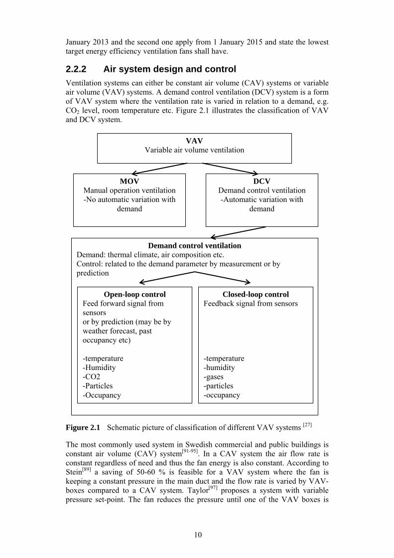
Ventilation systems can either be constant air volume (CAV) systems or variable air volume (VAV) systems. A demand control ventilation (DCV) system is a form of VAV system where the ventilation rate is varied in relation to a demand, e.g. CO2 level, room temperature etc. Figure 2.1 illustrates the classification of VAV and DCV system.

Figure 2.1 Schematic picture of classification of different VAV systems [27]

The most commonly used system in Swedish commercial and public buildings is constant air volume (CAV) system[91-95]. In a CAV system the air flow rate is constant regardless of need and thus the fan energy is also constant. According to Stein[89] a saving of 50-60 % is feasible for a VAV system where the fan is keeping a constant pressure in the main duct and the flow rate is varied by VAV-boxes compared to a CAV system. Taylor[97] proposes a system with variable pressure set-point. The fan reduces the pressure until one of the VAV boxes is

VAV Variable air volume ventilation

DCV Demand control ventilation -Automatic variation with

demand

MOV Manual operation ventilation -No automatic variation with

demand

Demand control ventilation Demand: thermal climate, air composition etc. Control: related to the demand parameter by measurement or by prediction

Open-loop control Feed forward signal from sensors or by prediction (may be by weather forecast, past occupancy etc) -temperature -Humidity -CO2 -Particles -Occupancy

Closed-loop control Feedback signal from sensors -temperature -humidity -gases -particles -occupancy

11

fully open. This method to control fans has proved to save energy. However, stability problems can occur. When the fan increases the pressure in the duct, the flow rate will also increase, and the VAV-box will start to close the damper in order to meet the desired flow rate. The control system will then detect a too high pressure and consequently give a signal to the fan to reduce the speed in order to reduce the duct pressure and the VAV-box will open again, and the oscillation continues. Thus stability must be considered when the control system is designed. The saving potential is estimated to 30-50 % compared to a VAV-system with a fixed pressure set-point. According to Roth the energy saving estimated for United States is 40-50 % with DCV[77] system compared to CAV system. To determine the flow rate carbon dioxide concentration can be measured. The method correlates well with the number of people present and concentration of other pollutants generated by people. A minimum flow rate is required in order to take care of pollutants not linked to people, such as pollutants originated from office equipment, emissions from building materials, furniture, etc. The total flow rate in a DCV system is less than in a CAV system and in addition to fan energy savings, savings for air cooling and air heating is also achieved. To rebuild a fan to a variable speed fan is easily done with a pressure sensor and a frequency converter. However, the rest of the system must also be considered to avoid comfort problem. Dampers and inlet devices must be suitable for variable flow in order to avoid noise and draft. Maripuu[55] specifies demands for a well functioning VAV system in office buildings with focus on simple system solutions. The number of control components is limited, dampers situated in ducts are avoided and an inlet device is constructed for variable flow rate irrespective of pressure in the duct. The flow rate is usually controlled by temperature, CO2-levels or occupancy. The above criteria and theories were tested in a field study[54] where a ventilation system in an office buildings was changed from a CAV system to DCV system. The results showed a fan energy reduction of 48 % (from 14.8 kWh/year/m2 to 7.7 kWh/year/m2). The same study reports an energy use in a newly build office building with a similar DCV system of 7.1 kWh/year/m2. This indicates that a retrofitted DCV system can have energy use on par with new installations. Fahlén[29] propose a system design where the components (air heater, air cooler, heat exchanger) of an air handling unit is situated in parallel. Increased internal loads in combination with better insulated buildings have reduced operating hours for air heaters and heat recovery units. Short operating hours combined with varying occupancy levels in office buildings provides a good basis for use of control on demand systems. In a traditional air-handling unit the air passes all components (air heaters, air coolers and heat recovery) regardless of whether heating or cooling is needed. These components cause a pressure drop in the system and as a consequence increased fan energy. Wulfinghoff argues against multi-zone central air handling systems which presently is the dominant type of HVAC for large buildings[104]. Wulfinghoff claims that they are inherently incapable of providing high level of comfort and good ventilation while operating with good energy efficiency. The desired solution is single zone systems. Problems associated with multi-zone VAV system

12

are reheat energy waste for space temperature control (centrally cooled air is reheated in the individual space to desired temperature), ventilation conflict with energy efficiency (efficient use of conditioned air requires tailored ventilation to each zone’s changing requirements), “dumping” of chilled air in VAV systems (at low cooling loads the air flow velocity is not high enough, the cooled air then falls directly to the floor causing discomfort), noise in VAV and induction systems (annoying flow noise as the damper closes), inability to isolate energy use from unoccupied zones, etc.

2.2.3 Damper authority

Lizardos[52] discuss damper authority. The total systems pressure drop to use when calculating the damper authority relates to the part of the system where the damper controls the flow. It is usually the pressure drop from a constant pressure point to the destination of the air flow. A damper authority of 30 - 50 % is recommended for good linear control of dampers with parallel blades. For dampers with opposed blades an authority of 10 - 15 % is recommended.

2.2.4 Fan efficiency

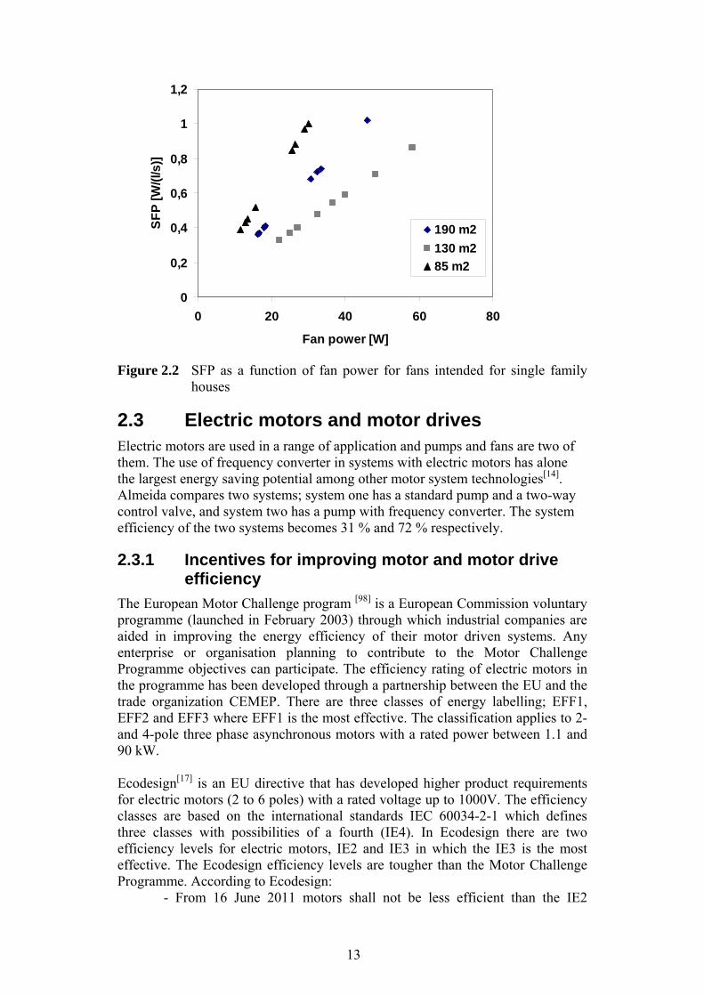
The manufactures data for fans does not always conform to how the fan performs in realty. This is due to several factors. In the manufacturers’ test process of the fan, not every wheel size presented in the data sheets is tested but calculated. This applies to both performance and sound[69]. In order to solve the problem where manufactures data could not be trusted the association Eurovent was formed. Eurovents members are national associations from 14 countries and the Swedish member is “Svensk ventilation”. Eurovent Certification[20] certifies manufactures data for air handling units and air conditioning equipment according to European and international standards. The aim of the certification is to build customer confidence by improving the reliability of manufacturers’ data. Thus, the customer can be sure that the purchased product will perform according to specified data. For the manufacturer the Eurovent Certification is the common platform where competition of performances can take place on comparable basis. The Swedish energy agency conducted 2010 a test of exhaust air fans for single-family houses[2]. In Figure 2.2 the SFP as a function of fan power for the tested fans is shown. The fans are divided into three categories according to house area indented for; 85 m2, for 130 m2 and 190 m2. In every category four fans have permanent magnet motor and four have induction motor. The result shows that the efficiency of the fans with EC-motors are almost three times higher than for the fans with EC-motor. In the Swedish building code the SFP recommended for exhaust fans is ≤ 0.6. In Figure 2.2 half of the fans have a SFP exceeding 0.6.

13

Figure 2.2 SFP as a function of fan power for fans intended for single family

houses

2.3 Electric motors and motor drives Electric motors are used in a range of application and pumps and fans are two of them. The use of frequency converter in systems with electric motors has alone the largest energy saving potential among other motor system technologies[14]. Almeida compares two systems; system one has a standard pump and a two-way control valve, and system two has a pump with frequency converter. The system efficiency of the two systems becomes 31 % and 72 % respectively.

2.3.1 Incentives for improving motor and motor drive efficiency

The European Motor Challenge program [98] is a European Commission voluntary programme (launched in February 2003) through which industrial companies are aided in improving the energy efficiency of their motor driven systems. Any enterprise or organisation planning to contribute to the Motor Challenge Programme objectives can participate. The efficiency rating of electric motors in the programme has been developed through a partnership between the EU and the trade organization CEMEP. There are three classes of energy labelling; EFF1, EFF2 and EFF3 where EFF1 is the most effective. The classification applies to 2- and 4-pole three phase asynchronous motors with a rated power between 1.1 and 90 kW. Ecodesign[17] is an EU directive that has developed higher product requirements for electric motors (2 to 6 poles) with a rated voltage up to 1000V. The efficiency classes are based on the international standards IEC 60034-2-1 which defines three classes with possibilities of a fourth (IE4). In Ecodesign there are two efficiency levels for electric motors, IE2 and IE3 in which the IE3 is the most effective. The Ecodesign efficiency levels are tougher than the Motor Challenge Programme. According to Ecodesign: - From 16 June 2011 motors shall not be less efficient than the IE2

0

0,2

0,4

0,6

0,8

1

1,2

0 20 40 60 80

Fan power [W]

SF

P [

W/(

l/s)]

190 m2

130 m2

85 m2

14

efficiency level. - From 1 January 2015 motors with a rated output of 7.5-375 kW shall not be less efficient than the IE3 efficiency level or meet the IE2 efficiency level and be equipped with a variable speed drive. - From 1 January 2017 all motors with a rated output of 0.75-375 kW shall not be less efficient than the IE3 efficiency level or meet the IE2 efficiency level and be equipped with a variable speed drive.

2.3.2 Motor type, frequency converters and other system efficiency factors

The efficiency of a motor system depends on several factors including the motor efficiency, motor speed control, proper sizing, power supply quality, distribution losses, mechanical transmission, maintenance practice and end-use mechanical efficiency (pump, fan, compressors etc.). The motor efficiency is dependant of what type of motor that is used. The most commonly used motor in the world is the induction (asynchronous) motor this is also true for the HVAC sector. The permanent magnet (PM) motor is becoming increasingly popular in HVAC application such as fan and pump motors. There are several kinds of PM motor but the most common used PM motor is the brushless direct current (BLDC) motor[39]. The stator lamination of a BLDC motor is similar to those of an induction motor. The main difference is the absence of shading coil slots and a presence of an asymmetric air-gap contour profile. The rotor consists of permanent magnets, typical ferrite, and the stator windings generate a rotating magnetic field. As the rotor rotates the stator windings are commutated, i.e. they are switched to be in phase with the poles in the rotor. In order to control the current to the stator rotor position need to be known. Electrically commutated motors (ECM or EC-motor) are a terminology that is specific for the HVAC industry[39]. Generally an EC-motor comprises a combination of a brushless DC motor and electronic converter used for variable speed operation of fans and pumps. BLDC motors behave like DC motors with brushes and when the motor is loaded the speed is proportional to the voltage and the torque is a linear function of current. BLDC motors with a power less than 0.75 kW has about 15 % [78] better efficiency than an induction motor with a frequency converter. For larger motors, the induction motor has increased efficiency and the efficiency difference of the BLDC motor and the induction motor decreases. The most common way of controlling a frequency converter is by using pulse width modulation (PWM). However, there are some problems associated with PWM. PWM causes increased levels of harmonics with increased copper and iron losses as a consequence. The motor efficiency is typical decreased by a factor 15-35 %. The life length of the motor can be influenced since the losses increase the motor temperature. There is an impedance difference between the motor and the cable. Depending on the wave form of the modulated voltage and the impedance difference between the cable and the motor the voltage wave can be reflected in the cable. At the motor the reflected voltage wave and the incoming voltage wave will be added according to the superposition principle with high amplitude voltage wave as a

15

consequence. The winding insulation is not capable of handling the high voltage and short circuit between the winding may appear. To avoid this kind of problem the cable between the motor and frequency converter should be kept short. Yet another problem connected with variable speed drives is shaft current. Due to capacitances between motor windings and motor frame, motor windings and rotor, rotor and motor frame and in bearings high frequency currents can occur. This high frequency current can shorten the life length of the bearings. Power harmonics can fed back to the electric grid and disrupt other equipment connected to the grid. To avoid these problems filters can be used[14]. Glover[33] deals with the problem with over dimensioning of electric motors. He estimates that only 20% of all pump motors operates at full load. Electric motors can operate for a limited time above rated power, and this can be exploited in the quest for energy efficiency. A limitation is the risk of motor overheating which can damage the motor insulation and bearings. Åström[107] describes the importance of optimal control of electric motors. By using an optimal combination of voltage and frequency in each operating mode losses in induction motors can be reduced significantly. Since this control method is effective at low motor load the problem of oversizing is reduced[106].

2.4 Literature review summary Electric motors use a substantial part of the electric energy in the world. Studies confirm that the single largest energy saving potential is using variable speed drives. Pumps and fans are centrifugal machines and therefore particularly suitable for variable speed drives. However, to achieve the full energy saving potential direct flow control by the pump or fan must be used. Today, most pump systems are temperature controlled using a shunt group or flow controlled by using a 2-way valve. When using control valves the pressure drop of the systems increases and in addition valve authority must be considered. The most commonly used ventilation system is the CAV system. With increasing internal loads, better building envelopes and varying occupancy levels demand control systems become more and more attractive. The overall conclusion is that large energy savings are achievable in ventilation system regarding heating, cooling and fan energy. Available statistics and knowledge about energy use for fans and pumps in commercial, public and residential buildings are limited, especially for residential buildings. The Swedish energy agency conducted a study with the aim to describe the energy use in commercial and public buildings. The next chapter summarizes the available statistics and information regarding energy use by pumps and fans in non-industrial buildings in Sweden.

16

17

3 Building related electric energy to pumps and fans in Sweden

This chapter provides an overview of the electrical energy to fans and pumps in non-industrial buildings in Sweden. The overview is based on available statistics, information found in reports and from Statistics Sweden. In some of the cases it has been difficult to find statistics and information. In this section the available information is put together and an estimated saving potential of electrical energy for pumps and fans in non-industrial buildings is made. Information regarding pumps and fans in commercial and public buildings (i.e. non industrial and non-residential buildings) is fairly good and described in the STIL2-reports[91-95]. In the case of multi- and single-family houses information is scarce and in many cases non-existing. The Swedish National Board of Housing, Building and Planning was commissioned by the Swedish government to examine and describe the Swedish building stock regarding energy use, technical status and indoor environment[73]. Unfortunately nothing about pump or fan operation is included in the study.

3.1 Energy use and conditioned floor area for non-industrial buildings

3.1.1 Energy use in non-industrial buildings

The building stock can be divided into different building categories. The Swedish Energy Agency and Statistics Sweden have defined a building sector that is called “residential and service sector etc.” (i.e. all non-industrial buildings). The post “etc.” includes recreational houses, agriculture and forestry and other service (water and waste plants, electrical plants, streetlights etc.) and use 13 % of the total supplied energy to the sector “residential and service sectors etc”[19]. Figure 3.1 shows the delivered energy to the Swedish non-industrial building stock 2009. Seen in a historical perspective the total use of energy has been more or less constant since the early 1970s. However, the distribution between the energy sources has changed considerably and particularly the use of oil has decreased substantially, while the use of bio fuels, district heating and electric energy have increased. In the 1970s district heating was based more or less solely on oil whereas in 2009 bio fuel and waste heat was about 77 % of the supplied fuels for district heating. The constant level of purchased energy since the 1970s should be compared with a 40 % increase of conditioned building area over the same period.

18

Figure 3.1 Delivered energy to the non-industrial building sector in Sweden 2009[19]

Electrical energy to the residential and service sector is about 70 TWh/year, about 45 % of all energy supplied. In Figure 3.2 the use of the delivered electric energy to the non-industrial building is shown. It is apparent that the main part is used for building operation.

Figure 3.2 Delivered electrical energy to the non-industrial building sector in

Sweden 2008[19]

About 42 % of the delivered electrical energy to non-industrial buildings is used as building operation and about 28 % and 30 % is household electricity and electricity for heating respectively. The electrical energy use increased between the 1970s and 1990s and has from the late 1990s been more or less stable. Electrical energy for heating has decreased while household electricity and the electricity for building operation have increased.

0

20

40

60

80

100

120

140

160

Delivered energy [TWh/year]

District heating

Electricity

Bio‐fuels

Other fuels

Oil products

0

10

20

30

40

50

60

70

80

Delivered electrical energy [TWh/year]

Electricity for heating

Electricity for household purpose

Electricity for building operation

19

The household electricity is the electricity used for lighting, white goods and appliances in residential buildings. The concept “electricity for building operation” is actually the residue in delivered electrical energy after subtract the household electricity and the electrical heating. Thus the post “electricity for building operation” contains a number of items other than what generally is considered as electricity for building operation. As an example the electrical energy used by the item “etc.” mentioned above. The electrical energy for building operation concerns principally:

Electricity pay for by the building owner of multifamily houses (landlord electricity)

Electricity pay for by the building owner of commercial and public buildings (landlord electricity)

Electricity pay for by the tenant in commercial and public buildings (business electricity)

The electrical energy for which the owner pays consists partly of the building services electricity (i.e. drive energy for pumps, fans, chillers for comfort cooling, control systems etc.) and partly of electrical energy used by lighting for stairwells, outdoor environments and shared laundry rooms etc. From the summary above it is clear that no uniform definitions of the electrical energy use exist in Sweden. The electrical energy use of a premise can be divided according to organizational division or functional division. Organizational division mean a division of energy pay for by the landlord and energy pay for by the tenant. Functional division mean a division of outdoor electricity (electricity for outdoor lighting, car heaters etc.) and building electricity (building services electricity and business electricity). In residential buildings, business electricity is denoted household electricity.

3.1.2 Conditioned floor area in non-industrial buildings

Different studies estimate conditioned floor areas and define building categories differently. In this chapter these differences are neglected since the purpose is to give an overview of pump and fan operation in non-industrial buildings. The building stock is divided according to:

Residential buildings Commercial and public buildings = Non-residential and non-industrial

buildings Industrial buildings

Industrial buildings are not considered in this study. Office buildings, schools, retail buildings, health care buildings, sport buildings etc. are included in the category commercial and public buildings. Residential buildings can be divided into single-family houses and multi-family houses. Some of the data in this study concerning pump and fan operation is more detailed for the three categories office, school and health care buildings than for the other commercial and public buildings.

20

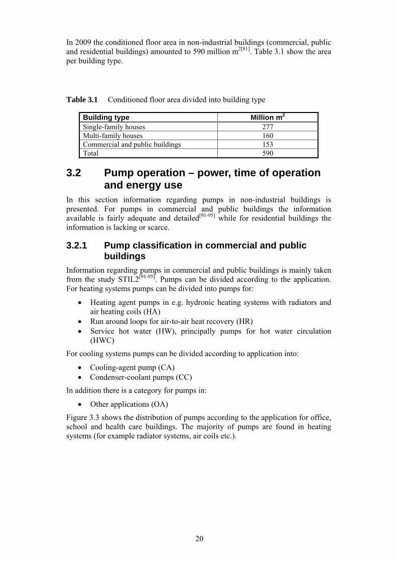
In 2009 the conditioned floor area in non-industrial buildings (commercial, public and residential buildings) amounted to 590 million m2[81]. Table 3.1 show the area per building type.

Table 3.1 Conditioned floor area divided into building type

Building type Million m2 Single-family houses 277Multi-family houses 160Commercial and public buildings 153Total 590

3.2 Pump operation – power, time of operation and energy use

In this section information regarding pumps in non-industrial buildings is presented. For pumps in commercial and public buildings the information available is fairly adequate and detailed[91-95] while for residential buildings the information is lacking or scarce.

3.2.1 Pump classification in commercial and public buildings

Information regarding pumps in commercial and public buildings is mainly taken from the study STIL2[91-95]. Pumps can be divided according to the application. For heating systems pumps can be divided into pumps for:

Heating agent pumps in e.g. hydronic heating systems with radiators and air heating coils (HA)

Run around loops for air-to-air heat recovery (HR) Service hot water (HW), principally pumps for hot water circulation

(HWC)

For cooling systems pumps can be divided according to application into:

Cooling-agent pump (CA) Condenser-coolant pumps (CC)

In addition there is a category for pumps in:

Other applications (OA)

Figure 3.3 shows the distribution of pumps according to the application for office, school and health care buildings. The majority of pumps are found in heating systems (for example radiator systems, air coils etc.).

21

Figure 3.3 Distribution of pumps per application and building type

3.2.2 Installed pump power in commercial and public buildings

Figure 3.4 show the measured or estimated pump power per application according to STIL2 for office, school and health care buildings. 81 % of the pumps have a pump power of less than 1 kW and 35 % of the pumps have a pump power of less than 150 W. Regardless of building type about a third of the pumps have a pump power between 150 W and 400 W.

Figure 3.4 Mean pump power per type of application in office, school and

health care building

HA HW CA CC HR OA

Mean pump power [kW]

0

0,5

1

1,5

2

2,5

3

3,5

4offices schools health caretotal

HA  HW CA CC HR OA 

22

Pumps in cooling applications tend to have a higher pump power than pumps in heating applications. This is partly due to larger fluid flows as a consequence of lower temperature differences compared to heating systems. Overall, pumps in school buildings seem to have lower pump power (due to smaller buildings and lower buildings and little use of cooling). Pumps in service hot water applications seem to be small regardless of what type of building they are situated in.

3.2.3 Pump operational time and pump energy in commercial and public buildings

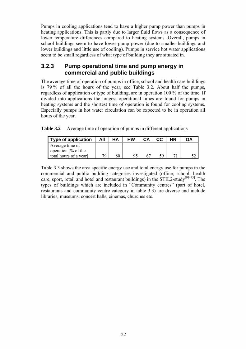
The average time of operation of pumps in office, school and health care buildings is 79 % of all the hours of the year, see Table 3.2. About half the pumps, regardless of application or type of building, are in operation 100 % of the time. If divided into applications the longest operational times are found for pumps in heating systems and the shortest time of operation is found for cooling systems. Especially pumps in hot water circulation can be expected to be in operation all hours of the year.

Table 3.2 Average time of operation of pumps in different applications

Type of application All HA HW CA CC HR OA Average time of operation [% of the total hours of a year] 79 80 95 67 59 71 52

Table 3.3 shows the area specific energy use and total energy use for pumps in the commercial and public building categories investigated (office, school, health care, sport, retail and hotel and restaurant buildings) in the STIL2-study[91-95]. The types of buildings which are included in “Community centres” (part of hotel, restaurants and community centre category in table 3.3) are diverse and include libraries, museums, concert halls, cinemas, churches etc.

23

Table 3.3 Area specific energy use and total energy use for pumps divided into building category for commercial and public buildings. Also the mean pump power per pump is included for office, school and health care buildings

Building category

Mean pump power

[kW/pump]

Area specific electrical energy

[kWh/year/m²]

Part of total electrical

energy use [%] (per

category excl. electrical heating)

Electricity use for pump

operation [TWh/year]

Office buildings

1.0 5.5 5.4 0.17

Schools

0.3 3.3 5.3 0.11

- Preschools 3.6 5.1 - Schools and high schools

3.2 5.2

Health care buildings

1.0 4.5 5.8 0.084

- Hospitals 5.4 6.4 - Service homes 2.4 4.0 Sports buildings - 16 12 0.072- Sport centres 2.0 3.5 - Ice skating halls 20 11 - Combination sports centres

23 15

- Swimming halls 28 17 Retail buildings - 6.4 3.7 0.093-Grocery shops 11.7 3.8 -Other 3.7 3.4 -Shopping arcades 6.7 4.6 Hotels, restaurants and community centres

- 4.8 3.8 0.056

-Hotel 5.5 3.4 -Restaurant 6.6 1.6 -Community centres

4.2 4.9

Mean value (area weighted)

5.1 Sum=0.585

Out of the inspected building categories sport buildings as a whole has the largest area specific pump electric energy use. This is a consequence of swimming halls and ice skating halls having a large pump energy use. The same holds for combination sport centres which can have swimming pool and other activities such as gymnasium or bowling alley. For Schools, sport centres (subcategory to sport buildings) and service homes the area specific pump energy is relatively low, as expected.

24

According to the Swedish energy agency the heated floor area for commercial and public sector in 2009 amounted to 153 million m2[81], including commercial areas in multifamily houses such as shops and hairdressers, but excluding housing in commercial buildings. The heated floor area for commercial and public buildings, including housing in these buildings, was 134 million m²[82] in 2009. The STIL2 Study reports 135 million m² in 2010[87]. The average area specific energy use for pump operation is 5.3 kWh/year/m2 which results in a total use of 0.72 TWh for the pumps in commercial and public buildings. The electric energy for pump operation has increased in the last two decades. A similar study as the STIL-2 study that was conducted 1992[34] reported an energy use for pump operation of 0.13 TWh/year for commercial and public buildings.

3.2.4 Installed pump power in residential buildings

In this section the pump energy in residential buildings is estimated. Since the information is scarce some assumptions have been made. The assumptions applied are for number of pumps per building and their sizes. Pump energy in single-family houses and multi-family houses can be calculated according to the following assumptions:

Single family houses with a hydronic heating system built 1990 or earlier has a pump for the heating system with a pump power of 100 W

Single family houses with a hydronic heating system built 1991 or later has a pump for the heating system with a pump power of 50 W

Multi-family houses with hydronic heating systems built 1990 or earlier has a pump for the heating system with a power of 250 W

Multi-family houses with hydronic heating systems built 1991 or later has a pump for the heating system with a power of 150 W

In the buildings where pump stops are applied these take place during four months (15th of May until 15th of September)

All multi-family houses have pumps for hot water circulation with a pump power of 100 W

The number of single-family houses in Sweden is increasing. According to Statistic Sweden the number of single-family houses was 1.997 millions in the beginning of 2010[88]. In the beginning of 1991 the number of single-family houses amounted to 1.613 million m2[81]. In 2004 the number of multi-family houses in Sweden was about 135 000, which is 10 000 more than 1988[68].

3.2.5 Pump operational time and pump energy in residential buildings

Over 90 % of the area in multi-family houses have hydronic heating system[19] and therefore it is assumed that 90 % of the multi-family houses have a hydronic heating system. Further it is assumed that in 80 % of the multi-family houses practice pump stop during four months of the year. With the assumptions made, pumps in multifamily houses use about 0.31 TWh per year. In single-family houses two thirds of the buildings have non-electric based hydronic heating systems. One third of the single-family houses in Sweden are heated by electricity, whereof half has a hydronic heating system[18].This

25

implicates that over 80 % of the single-family houses in Sweden have a hydronic heating system. In about one third of the single-family houses with hydronic heating system pump stop is practised[99]. With the assumptions given above pumps in single-family houses use about 1.16 TWh per year.

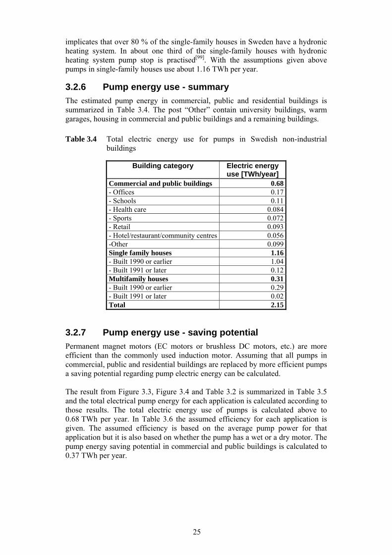
3.2.6 Pump energy use - summary

The estimated pump energy in commercial, public and residential buildings is summarized in Table 3.4. The post “Other” contain university buildings, warm garages, housing in commercial and public buildings and a remaining buildings.

Table 3.4 Total electric energy use for pumps in Swedish non-industrial buildings

Building category Electric energy use [TWh/year]

Commercial and public buildings 0.68 - Offices 0.17 - Schools 0.11 - Health care 0.084 - Sports 0.072 - Retail 0.093 - Hotel/restaurant/community centres 0.056 -Other 0.099 Single family houses 1.16 - Built 1990 or earlier 1.04 - Built 1991 or later 0.12 Multifamily houses 0.31 - Built 1990 or earlier 0.29 - Built 1991 or later 0.02 Total 2.15

3.2.7 Pump energy use - saving potential

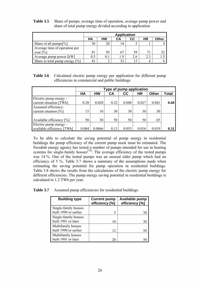
Permanent magnet motors (EC motors or brushless DC motors, etc.) are more efficient than the commonly used induction motor. Assuming that all pumps in commercial, public and residential buildings are replaced by more efficient pumps a saving potential regarding pump electric energy can be calculated. The result from Figure 3.3, Figure 3.4 and Table 3.2 is summarized in Table 3.5 and the total electrical pump energy for each application is calculated according to those results. The total electric energy use of pumps is calculated above to 0.68 TWh per year. In Table 3.6 the assumed efficiency for each application is given. The assumed efficiency is based on the average pump power for that application but it is also based on whether the pump has a wet or a dry motor. The pump energy saving potential in commercial and public buildings is calculated to 0.37 TWh per year.

26

Table 3.5 Share of pumps, average time of operation, average pump power and share of total pump energy divided according to application

Application HA HW CA CC HR Other

Share of all pumps[%] 56 20 14 5 1 4Average time of operation per year [%] 81 95 67 59 71 52Average pump power [kW] 0.5 0.1 1.9 2.6 2.3 1.5Share to total pump energy [%] 41 3 33 13 4 6

Table 3.6 Calculated electric pump energy per application for different pump efficiencies in commercial and public buildings

Type of pump application

HA HW CA CC HR Other TotalElectric pump energy - current situation [TWh] 0.28 0.020 0.22 0.088 0.027 0.041 0.68Assumed efficiency- current situation [%] 15 10 30 30 30 30 Available efficiency [%] 50 30 50 50 50 65

0.31Electric pump energy – available efficiency [TWh] 0.084 0.0066 0.13 0.053 0.016 0.019 To be able to calculate the saving potential of pump energy in residential buildings the pump efficiency of the current pump stock must be estimated. The Swedish energy agency has tested a number of pumps intended for use in heating systems for single-family houses[79]. The average efficiency of the tested pumps was 14 %. One of the tested pumps was an unused older pump which had an efficiency of 5 %. Table 3.7 shows a summary of the assumptions made when estimating the saving potential for pump operation in residential buildings. Table 3.8 shows the results from the calculations of the electric pump energy for different efficiencies. The pump energy saving potential in residential buildings is calculated to 1.2 TWh per year.

Table 3.7 Assumed pump efficiencies for residential buildings

Building type Current pump efficiency [%]

Available pump efficiency [%]

Single-family houses built 1990 or earlier 5

30

Single-family houses built 1991 or later 10

30

Multifamily houses built 1990 or earlier 12

50

Multifamily houses built 1991 or later 20

50

27

Table 3.8 Electric pump energy use in residential buildings calculated with efficiencies from Table 3.7

Building type Electric pump energy use with current

efficiency [TWh/year]

Electric pump energy use with state of the art

efficiency [TWh/year] Single-family houses built 1990 or earlier 1.04

0.17

Single-family houses built 1991 or later 0.12

0.040

Multifamily houses built 1990 or earlier 0.29

0.070

Multifamily houses built 1991 or later 0.02

0.0080

Total 1.47 0.29 The saving potential for pumps in commercial, public and residential buildings is calculated to 1.6 TWh per year if all pumps are exchanged to pumps with state of the art efficiency. This corresponds to 73 % of the electricity use of pumps today.

3.3 Fan operation – power, time of operation and energy use

Fans in non-industrial buildings use more than 3 % of the Swedish electrical energy use. Into relation to the wind power production which supplied about 2.5 % of the Swedish electricity 2010 the fan part is substantial. In the sector residential, commercial and public buildings (i.e. non-industrial buildings) fans use 25 % of the total electricity use[18-19]. In this chapter a summary of the information regarding fan operation in commercial, public and residential buildings is given. As the information regarding fan operation in residential buildings is scarce, fan operation in commercial and a public building is mainly discussed based on the investigation STIL2[91-95].

3.3.1 Fan classification in commercial and public buildings

In STIL2[91-95] the fans are divided according to the type of air handling system they are situated in:

CAV System with constant supply and constant return air flow rate and heat recovery, Constant Air Volume.

VAV System with heat recovery and variable supply and return air flow rate, Variable Air Volume.

SEF Mechanical ventilation without heat recovery (supply and exhaust fan)

EF Fan on return side (only exhaust fan). NV Natural ventilation Other

Figure 3.5 shows the distribution of air handling systems for office, school and health care buildings.

28

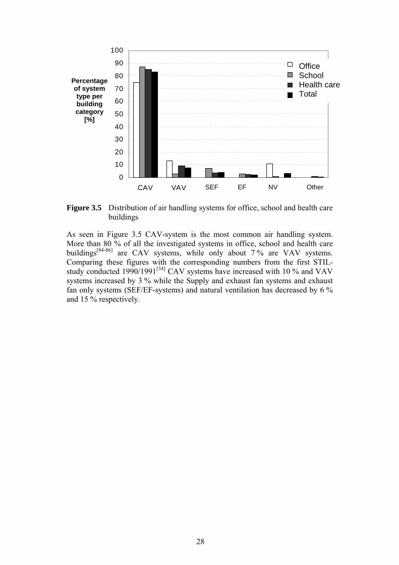
Figure 3.5 Distribution of air handling systems for office, school and health care

buildings

As seen in Figure 3.5 CAV-system is the most common air handling system. More than 80 % of all the investigated systems in office, school and health care buildings[84-86] are CAV systems, while only about 7 % are VAV systems. Comparing these figures with the corresponding numbers from the first STIL-study conducted 1990/1991[34] CAV systems have increased with 10 % and VAV systems increased by 3 % while the Supply and exhaust fan systems and exhaust fan only systems (SEF/EF-systems) and natural ventilation has decreased by 6 % and 15 % respectively.

0

10

20

30

40

50

60

70

80

90

100

CAV VAV TF FF Självdrag Annat

An

del

i v

arj

e lo

kalk

ate

go

ri [%

] kontor

skolor

vård

totalt

Office School Health care Total

Percentage of system type per building category

[%]

Other NV EF SEF

29

3.3.2 Installed fan power, specific fan power and energy use in commercial and public buildings

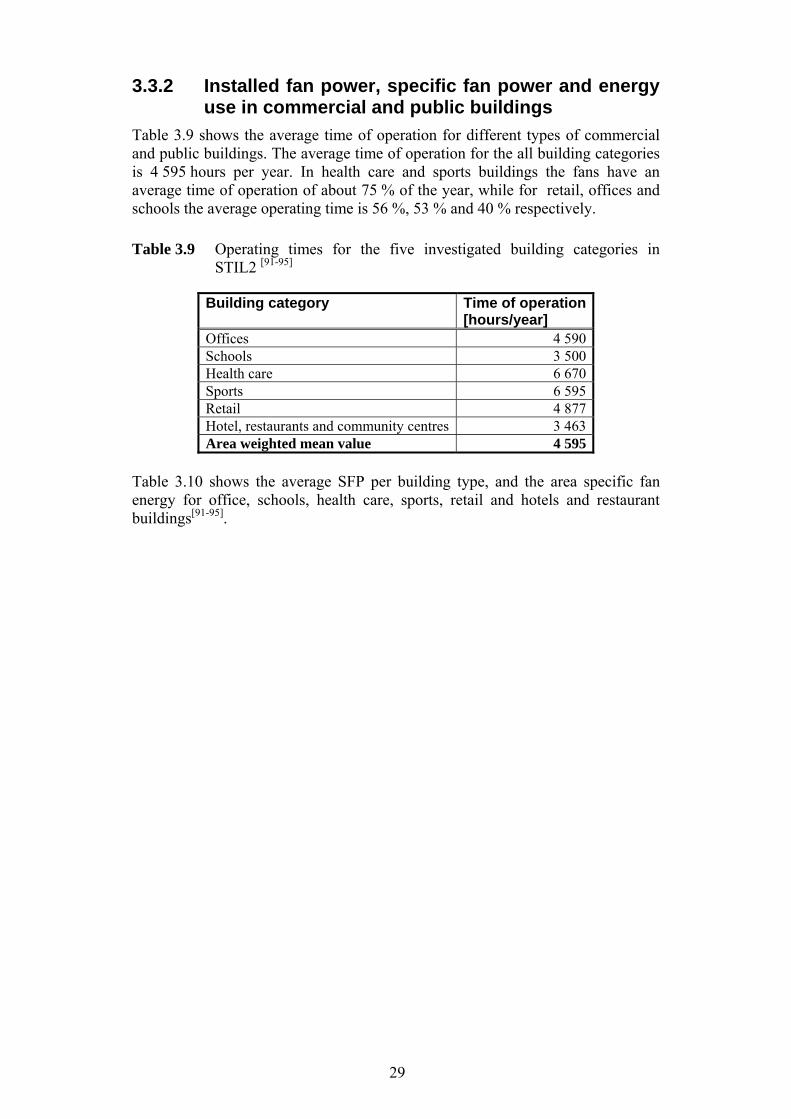
Table 3.9 shows the average time of operation for different types of commercial and public buildings. The average time of operation for the all building categories is 4 595 hours per year. In health care and sports buildings the fans have an average time of operation of about 75 % of the year, while for retail, offices and schools the average operating time is 56 %, 53 % and 40 % respectively.

Table 3.9 Operating times for the five investigated building categories in STIL2 [91-95]

Building category Time of operation [hours/year]

Offices 4 590 Schools 3 500 Health care 6 670 Sports 6 595 Retail 4 877 Hotel, restaurants and community centres 3 463 Area weighted mean value 4 595

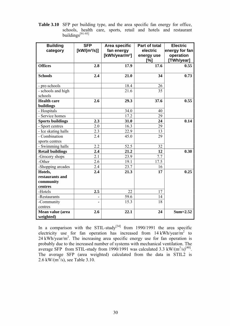
Table 3.10 shows the average SFP per building type, and the area specific fan energy for office, schools, health care, sports, retail and hotels and restaurant buildings[91-95].

30

Table 3.10 SFP per building type, and the area specific fan energy for office, schools, health care, sports, retail and hotels and restaurant buildings[91-95]

Building category

SFP [kW/(m³/s)]

Area specific fan energy

[kWh/year/m²]

Part of total electric

energy use [%]

Electric energy for fan

operation [TWh/year]

Offices

2.8 17.9 17.6 0.55

Schools

2.4 21.0 34 0.73

- pre-schools 18.4 26- schools and high schools

21.6 35

Health care buildings

2.6 29.3 37.6 0.55

- Hospitals 34.0 40- Service homes 17.2 29Sports buildings 2.3 31.0 24 0.14- Sport centres 2.0 16.3 29- Ice skating halls 2.3 22.9 13- Combination sports centres

2.4 45.0 29

- Swimming halls 2.2 52.5 32Retail buildings 2.4 21.2 12 0.30-Grocery shops 2.1 23.9 7.7-Other 2.6 19.1 17.5-Shopping arcades 2.4 23.7 16Hotels, restaurants and community centres

2.4 21.3 17 0.25

-Hotels 2.5 22 17-Restaurants - 59.6 14-Community centres

- 15.3 18

Mean value (area weighted)

2.6 22.1 24 Sum=2.52

In a comparison with the STIL-study[34] from 1990/1991 the area specific electricity use for fan operation has increased from 14 kWh/year/m2 to 24 kWh/year/m2. The increasing area specific energy use for fan operation is probably due to the increased number of systems with mechanical ventilation. The average SFP from STIL-study from 1990/1991 was calculated 3.3 kW/(m3/s)[40]. The average SFP (area weighted) calculated from the data in STIL2 is 2.6 kW/(m3/s), see Table 3.10.

31

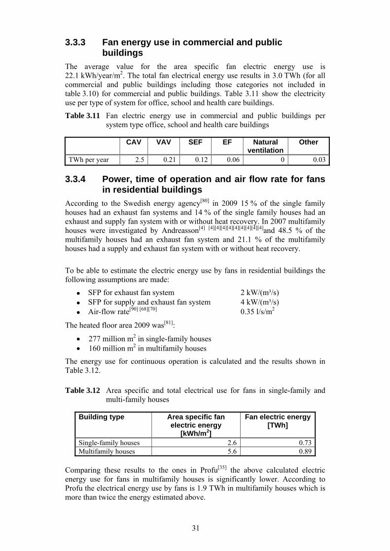
3.3.3 Fan energy use in commercial and public buildings

The average value for the area specific fan electric energy use is 22.1 kWh/year/m2. The total fan electrical energy use results in 3.0 TWh (for all commercial and public buildings including those categories not included in table 3.10) for commercial and public buildings. Table 3.11 show the electricity use per type of system for office, school and health care buildings.

Table 3.11 Fan electric energy use in commercial and public buildings per system type office, school and health care buildings

CAV VAV SEF EF Natural ventilation

Other

TWh per year 2.5 0.21 0.12 0.06 0 0.03

3.3.4 Power, time of operation and air flow rate for fans in residential buildings

According to the Swedish energy agency[80] in 2009 15 % of the single family houses had an exhaust fan systems and 14 % of the single family houses had an exhaust and supply fan system with or without heat recovery. In 2007 multifamily houses were investigated by Andreasson[4] [4][4][4][4][4][4][4][4][4]and 48.5 % of the multifamily houses had an exhaust fan system and 21.1 % of the multifamily houses had a supply and exhaust fan system with or without heat recovery.

To be able to estimate the electric energy use by fans in residential buildings the following assumptions are made:

SFP for exhaust fan system 2 kW/(m³/s) SFP for supply and exhaust fan system 4 kW/(m³/s) Air-flow rate[90] [68][70] 0.35 l/s/m2

The heated floor area 2009 was[81]:

277 million m2 in single-family houses 160 million m2 in multifamily houses

The energy use for continuous operation is calculated and the results shown in Table 3.12.

Table 3.12 Area specific and total electrical use for fans in single-family and multi-family houses

Building type Area specific fan electric energy

[kWh/m2]

Fan electric energy [TWh]

Single-family houses 2.6 0.73 Multifamily houses 5.6 0.89

Comparing these results to the ones in Profu[35] the above calculated electric energy use for fans in multifamily houses is significantly lower. According to Profu the electrical energy use by fans is 1.9 TWh in multifamily houses which is more than twice the energy estimated above.

32

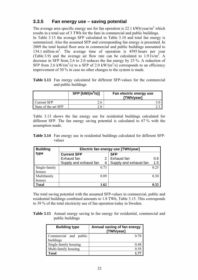
3.3.5 Fan energy use – saving potential

The average area specific energy use for fan operation is 22.1 kWh/year/m2 which results in a total use of 3 TWh for the fans in commercial and public buildings. In Table 3.13 the average SFP calculated in Table 3.10 and total fan energy is summarized. Also the assumed SFP and corresponding fan energy is presented. In 2009 the total heated floor area in commercial and public buildings amounted to 134.1 million m2. The average time of operation is 4595 hours per year (Table 3.9) and the average air flow rate can be calculated to 1.9 l/s/m2. A decrease in SFP from 2.6 to 2.0 reduces the fan energy by 23 %. A reduction of SFP from 2.6 kW/(m3/s) to a SFP of 2.0 kW/(m3/s) corresponds to an efficiency improvement of 30 % in case no other changes to the system is made.

Table 3.13 Fan energy calculated for different SFP-values for the commercial and public buildings

SFP [kW/(m3/s)] Fan electric energy use [TWh/year]

Current SFP 2.6 3.0 State of the art SFP 2.0 2.3

Table 3.13 shows the fan energy use for residential buildings calculated for different SFP. The fan energy saving potential is calculated to 67 % with the assumption made.

Table 3.14 Fan energy use in residential buildings calculated for different SFP-values

Building type

Electric fan energy use [TWh/year]

Current SFP Exhaust fan Supply and exhaust fan

24

SFP Exhaust fan Supply and exhaust fan

0.6 1.5

Single-family houses

0.73 0.25

Multifamily houses

0.89 0.30

Total 1.62 0.55 The total saving potential with the assumed SFP-values in commercial, public and residential buildings combined amounts to 1.8 TWh, Table 3.15. This corresponds to 39 % of the total electricity use of fan operation today in Sweden.

Table 3.15 Annual energy saving in fan energy for residential, commercial and public buildings

Building type Annual saving of fan energy [TWh/year]

Commercial and public buildings

0.70

Single-family housing 0.48 Multi-family housing 0.59 Total 1.77

33

3.4 Pump and fan energy use - summary The saving potential for pump and fan operation is comparable in size. Worth noticing is that for pumps more than 75 % of the saving potential is from the residential building sector. The number of single-family houses is almost 2 million, which of more that 80 % have hydronic heating system. Generally small pumps have lower efficiency compared to the pumps used in the larger applications. The availability of efficient small pumps has been low and many of the small pumps used in single family houses in Sweden have poor efficiency. The saving potential discussed in this chapter is based on assumptions regarding the efficiency of pump and fan operation in buildings. In the following chapters current HVAC system design and possible future HVAC system designs are discussed and modelled with the aim of increasing the knowledge of the saving potential at system level.

34

35

4 Current HVAC system design - Pump and fan duty

As previously noted the energy use for pumps, fans, heating and cooling in buildings is substantial. The Swedish parliament launched a national target to reduce the energy use by 2050 by 50 %. As a consequence the energy for fans, pumps, heating and cooling also needs to be reduced by 50 %. At the same time the requirement on indoor climate tends to be tougher both regarding thermal comfort as well as air quality and possibilities for individual control of temperature and ventilation. Improvement of building envelopes and increased internal loads call for shifting focus from heating to cooling and to drive power for fans and pumps. In order to understand what energy saving potential is feasible the design criteria for HVAC systems today must be known. The heating or cooling demand of a building can be provided by an all-air system, air-water system, water-air system or all-water system.

4.1 Design criteria The specific fan power (SFP), equation 4.1 and the specific pump power (SPP), equation 4.2 are two parameters that are useful in the design process as they quantify the energy efficiency of the distribution system including the fan and pump respectively. The parameters state what fan or pump power is needed per unit flow rate and have the unit [kW/(m3/s)]. If assuming a balanced supply and exhaust air and after simplifying equation 4.2 the SFP can be expressed as the sum of the fan pressure rise divided by the fan efficiency, equation 4.3. For one branch in a pump system (i.e. for one pump) the SPP can be expressed according to equation 4.4.

∑

(4.1)

∑

(4.2)

∑ (4.3)

(4.4)

To make a distribution system more energy efficient, which is to reduce the SFP or SPP, the system pressure drop can be reduced and/or the pump or fan efficiency can be increased. As a way of defining system efficiency, SFP has been used in Sweden for many years. Typical values of the SFP for new buildings are 1.5-2.0 kW/(m3/s) and 2.0-2.5 kW/(m3/s) for refurbishment of existing buildings. Recommended SFP values from the Swedish building code is given in Table 4.1 [90]. The values are for newly built houses. In case of refurbishment if both the air handling unit and the distributions system is refurbished the SFP in Table 4.1 is recommended and in case of refurbishment of only the air handling unit SFP values in Table 4.1 is recommended for the air handling unit alone.

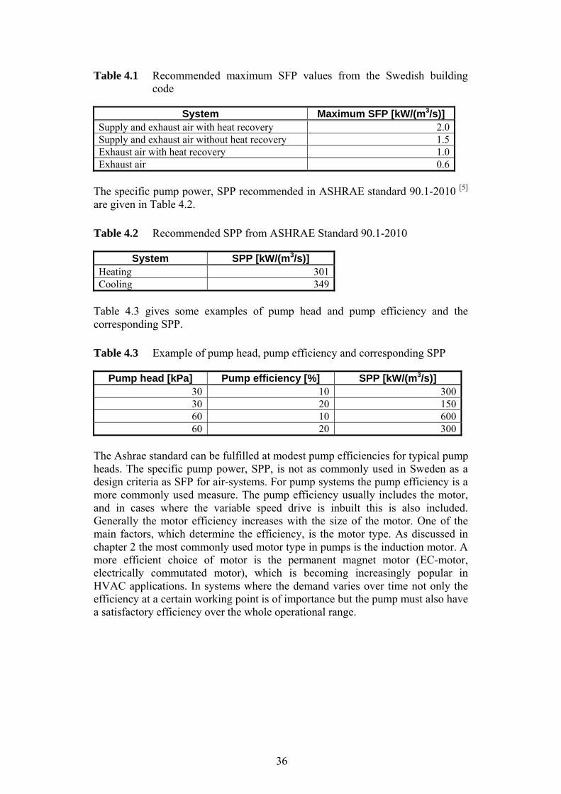
36

Table 4.1 Recommended maximum SFP values from the Swedish building code

System Maximum SFP [kW/(m3/s)] Supply and exhaust air with heat recovery 2.0 Supply and exhaust air without heat recovery 1.5 Exhaust air with heat recovery 1.0 Exhaust air 0.6

The specific pump power, SPP recommended in ASHRAE standard 90.1-2010 [5] are given in Table 4.2.

Table 4.2 Recommended SPP from ASHRAE Standard 90.1-2010

System SPP [kW/(m3/s)] Heating 301Cooling 349

Table 4.3 gives some examples of pump head and pump efficiency and the corresponding SPP.

Table 4.3 Example of pump head, pump efficiency and corresponding SPP

Pump head [kPa] Pump efficiency [%] SPP [kW/(m3/s)] 30 10 300 30 20 150 60 10 600 60 20 300

The Ashrae standard can be fulfilled at modest pump efficiencies for typical pump heads. The specific pump power, SPP, is not as commonly used in Sweden as a design criteria as SFP for air-systems. For pump systems the pump efficiency is a more commonly used measure. The pump efficiency usually includes the motor, and in cases where the variable speed drive is inbuilt this is also included. Generally the motor efficiency increases with the size of the motor. One of the main factors, which determine the efficiency, is the motor type. As discussed in chapter 2 the most commonly used motor type in pumps is the induction motor. A more efficient choice of motor is the permanent magnet motor (EC-motor, electrically commutated motor), which is becoming increasingly popular in HVAC applications. In systems where the demand varies over time not only the efficiency at a certain working point is of importance but the pump must also have a satisfactory efficiency over the whole operational range.

37

Figure 4.1 shows an example of pump efficiencies for three pumps, two with permanent magnet motors and one with induction motor. Two of the pumps are of equal size in terms of flow rate and differential pressure (pump II and pump III). However, the pump with EC-motor (II) has an input power of about 40 % less than the pump with induction motor (III). Two of the pumps are of equal sizes in terms of input power (pump I and pump III). As expected the efficiency is much higher for the pump with EC-motor (I) and thus the performance in flow rate and differential pressure is higher.

Figure 4.1 Pump efficiencies as a function of flow rate for the three different

pumps

4.2 Liquid systems Figure 4.2a-c shows the system layout for the most common pump system designs. In the system in Figure 4.2a-b, the heating capacity is controlled by a variable temperature obtained by mixing supply water with a temperature tsupply, return water with a temperature treturn, to the desired inlet temperature tinlet. The supply temperature is typically a function of the outdoor temperature. The control valve controls the mixing degree of return water. In this case the differential pressure from the pump must overcome not only the pressure drop from the piping and heating units, but also that of the balancing and the control valves. For the system design in Figure 4.2a the flow rate is constant on the primary (heat source side) and the secondary side (heat emitting side). This type of system solution is often used when a high return temperature is desirable, for example in boiler applications. For the system design in Figure 4.2b the flow rate is constant on the secondary side (heat emitting side) while on the primary side (heat source) the flow rate is variable. This type of system design is common when a low return temperature is desirable, for example when the heat source is district heating.

Pump III

Pump II

Pump I

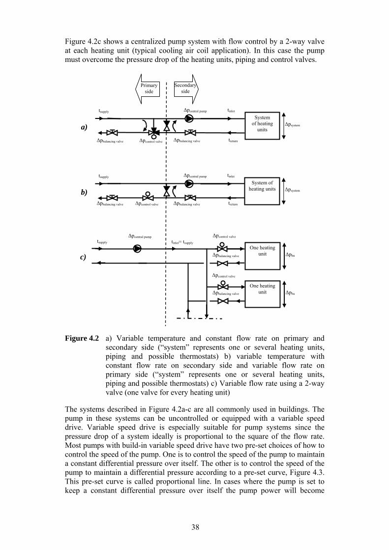
38

Figure 4.2c shows a centralized pump system with flow control by a 2-way valve at each heating unit (typical cooling air coil application). In this case the pump must overcome the pressure drop of the heating units, piping and control valves.

Figure 4.2 a) Variable temperature and constant flow rate on primary and

secondary side (“system” represents one or several heating units, piping and possible thermostats) b) variable temperature with constant flow rate on secondary side and variable flow rate on primary side (“system” represents one or several heating units, piping and possible thermostats) c) Variable flow rate using a 2-way valve (one valve for every heating unit)

The systems described in Figure 4.2a-c are all commonly used in buildings. The pump in these systems can be uncontrolled or equipped with a variable speed drive. Variable speed drive is especially suitable for pump systems since the pressure drop of a system ideally is proportional to the square of the flow rate. Most pumps with build-in variable speed drive have two pre-set choices of how to control the speed of the pump. One is to control the speed of the pump to maintain a constant differential pressure over itself. The other is to control the speed of the pump to maintain a differential pressure according to a pre-set curve, Figure 4.3. This pre-set curve is called proportional line. In cases where the pump is set to keep a constant differential pressure over itself the pump power will become

Secondary side

Primary side

Δpsystem

Δpbalancing valve Δpcontrol valve Δpbalancing valve

tinlet Δpcentral pump

treturn

tsupply

System of heating units b)

Δpsystem

Δpbalancing valve Δpcontrol valve Δpbalancing valve

tinlet Δpcentral pump

treturn

tsupply

System of heating

units a)

c)

Δpcontrol valve Δpcentral pump

tsupply

One heating unit Δphu

Δpcontrol valve

One heating unit Δphu Δpbalancing valve

Δpbalancing valve

tinlet= tsupply

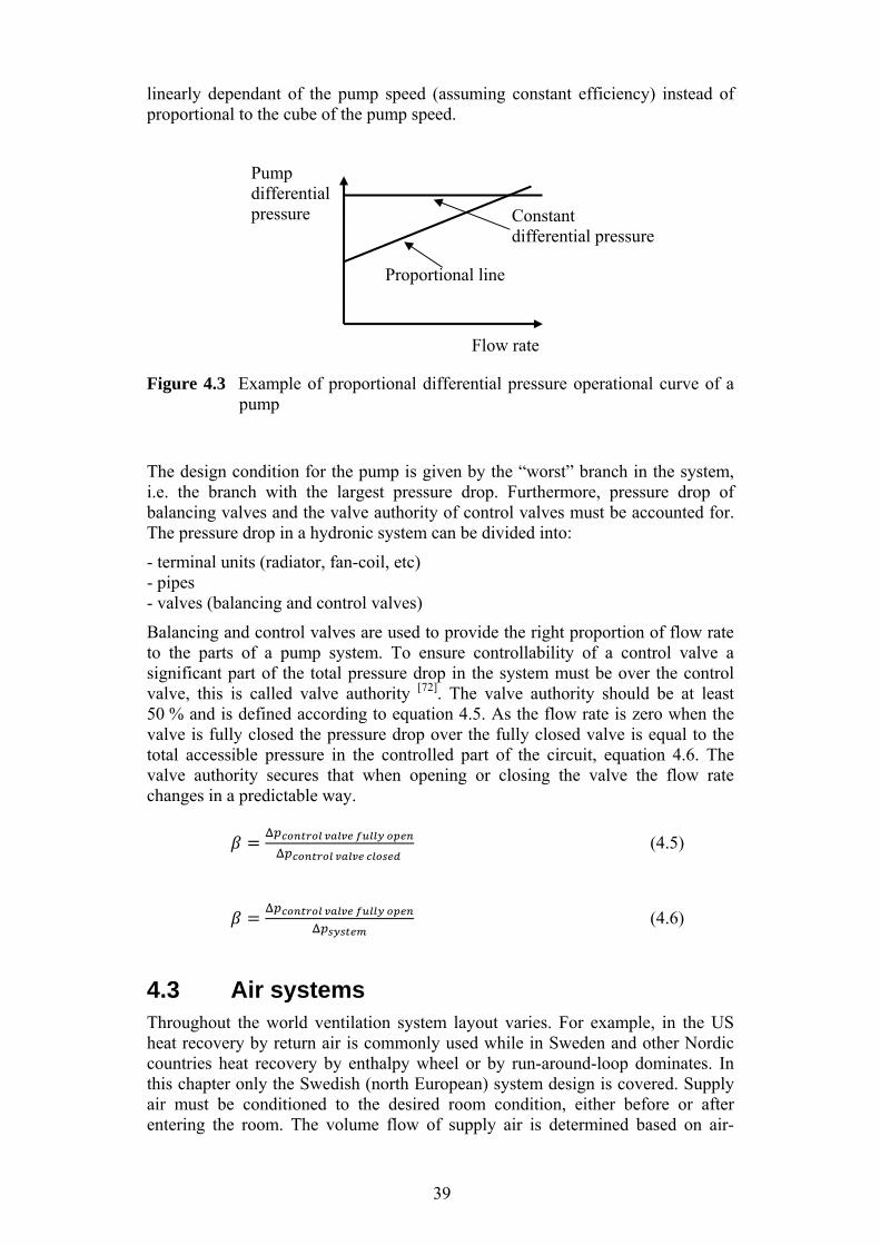
39

linearly dependant of the pump speed (assuming constant efficiency) instead of proportional to the cube of the pump speed.

Figure 4.3 Example of proportional differential pressure operational curve of a pump

The design condition for the pump is given by the “worst” branch in the system, i.e. the branch with the largest pressure drop. Furthermore, pressure drop of balancing valves and the valve authority of control valves must be accounted for. The pressure drop in a hydronic system can be divided into:

- terminal units (radiator, fan-coil, etc) - pipes - valves (balancing and control valves)

Balancing and control valves are used to provide the right proportion of flow rate to the parts of a pump system. To ensure controllability of a control valve a significant part of the total pressure drop in the system must be over the control valve, this is called valve authority [72]. The valve authority should be at least 50 % and is defined according to equation 4.5. As the flow rate is zero when the valve is fully closed the pressure drop over the fully closed valve is equal to the total accessible pressure in the controlled part of the circuit, equation 4.6. The valve authority secures that when opening or closing the valve the flow rate changes in a predictable way.

(4.5)

(4.6)

4.3 Air systems Throughout the world ventilation system layout varies. For example, in the US heat recovery by return air is commonly used while in Sweden and other Nordic countries heat recovery by enthalpy wheel or by run-around-loop dominates. In this chapter only the Swedish (north European) system design is covered. Supply air must be conditioned to the desired room condition, either before or after entering the room. The volume flow of supply air is determined based on air-

Flow rate

Pump differential pressure

Proportional line

Constant differential pressure

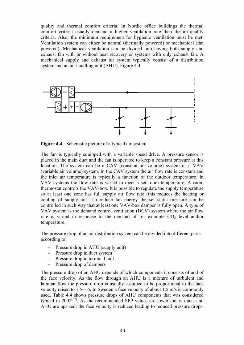
40

quality and thermal comfort criteria. In Nordic office buildings the thermal comfort criteria usually demand a higher ventilation rate than the air-quality criteria. Also, the minimum requirement for hygienic ventilation must be met. Ventilation system can either be natural (thermally powered) or mechanical (fan powered). Mechanical ventilation can be divided into having both supply and exhaust fan with or without heat recovery or systems with only exhaust fan. A mechanical supply and exhaust air system typically consist of a distribution system and an air handling unit (AHU), Figure 4.4.

Figure 4.4 Schematic picture of a typical air system

The fan is typically equipped with a variable speed drive. A pressure sensor is placed in the main duct and the fan is operated to keep a constant pressure at this location. The system can be a CAV (constant air volume) system or a VAV (variable air volume) system. In the CAV system the air flow rate is constant and the inlet air temperature is typically a function of the outdoor temperature. In VAV systems the flow rate is varied to meet a set room temperature. A room thermostat controls the VAV-box. It is possible to regulate the supply temperature so at least one zone has full supply air flow rate (this reduces the heating or cooling of supply air). To reduce fan energy the set static pressure can be controlled in such way that at least one VAV-box damper is fully open. A type of VAV system is the demand control ventilation (DCV) system where the air flow rate is varied in response to the demand of for example CO2 level and/or temperature. The pressure drop of an air distribution system can be divided into different parts according to:

- Pressure drop in AHU (supply unit) - Pressure drop in duct system - Pressure drop in terminal unit - Pressure drop of dampers

The pressure drop of an AHU depends of which components it consists of and of the face velocity. As the flow through an AHU is a mixture of turbulent and laminar flow the pressure drop is usually assumed to be proportional to the face velocity raised to 1.5-1.6. In Sweden a face velocity of about 1.5 m/s is commonly used. Table 4.4 shows pressure drops of AHU components that was considered typical in 2002[67]. As the recommended SFP values are lower today, ducts and AHU are upsized; the face velocity is reduced leading to reduced pressure drops.

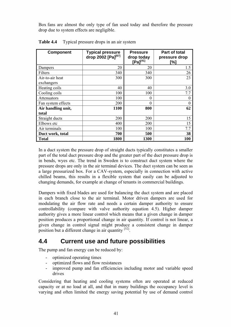
41

Box fans are almost the only type of fan used today and therefore the pressure drop due to system effects are negligible.

Table 4.4 Typical pressure drops in an air system

Component Typical pressure drop 2002 [Pa][67]

Pressure drop today

[Pa][41]

Part of total pressure drop

[%] Dampers 20 20 1.5 Filters 340 340 26 Air-to-air heat exchangers

300 300 23

Heating coils 40 40 3.0 Cooling coils 100 100 7.7 Attenuators 100 0 0 Fan system effects 200 0 0 Air handling unit, total

1100 800 62

Straight ducts 200 200 15 Elbows etc 400 200 15 Air terminals 100 100 7.7 Duct work, total 700 500 38 Total 1800 1300 100 In a duct system the pressure drop of straight ducts typically constitutes a smaller part of the total duct pressure drop and the greater part of the duct pressure drop is in bends, wyes etc. The trend in Sweden is to construct duct system where the pressure drops are only in the air terminal devices. The duct system can be seen as a large pressurized box. For a CAV-system, especially in connection with active chilled beams, this results in a flexible system that easily can be adjusted to changing demands, for example at change of tenants in commercial buildings. Dampers with fixed blades are used for balancing the duct system and are placed in each branch close to the air terminal. Motor driven dampers are used for modulating the air flow rate and needs a certain damper authority to ensure controllability (compare with valve authority equation 4.5). Higher damper authority gives a more linear control which means that a given change in damper position produces a proportional change in air quantity. If control is not linear, a given change in control signal might produce a consistent change in damper position but a different change in air quantity [52].

4.4 Current use and future possibilities The pump and fan energy can be reduced by:

- optimized operating times - optimized flows and flow resistances - improved pump and fan efficiencies including motor and variable speed

drives

Considering that heating and cooling systems often are operated at reduced capacity or at no load at all, and that in many buildings the occupancy level is varying and often limited the energy saving potential by use of demand control

42

systems is large. Demands varies locally in rooms/zones and by delivering the right heating/cooling and air flow rates at the right time and place electric as well as heating energy can be saved. The available technology for variable speed drive makes it possible for the distribution of flow to be delivered by direct flow control by variable speed pumps and fans. In that way control dampers and valves are not needed and a substantial part of the system pressure drop could be reduced. If systems are becoming more independent of “pressure”, the conventional view of pumps and fans and their motors need to be reconsidered.

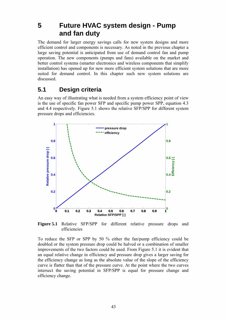
43

5 Future HVAC system design - Pump and fan duty

The demand for larger energy savings calls for new system designs and more efficient control and components is necessary. As noted in the previous chapter a large saving potential is anticipated from use of demand control fan and pump operation. The new components (pumps and fans) available on the market and better control systems (smarter electronics and wireless components that simplify installation) has opened up for new more efficient system solutions that are more suited for demand control. In this chapter such new system solutions are discussed.

5.1 Design criteria An easy way of illustrating what is needed from a system efficiency point of view is the use of specific fan power SFP and specific pump power SPP, equation 4.3 and 4.4 respectively. Figure 5.1 shows the relative SFP/SPP for different system pressure drops and efficiencies.

Figure 5.1 Relative SFP/SPP for different relative pressure drops and

efficiencies

To reduce the SFP or SPP by 50 % either the fan/pump efficiency could be doubled or the system pressure drop could be halved or a combination of smaller improvements of the two factors could be used. From Figure 5.1 it is evident that an equal relative change in efficiency and pressure drop gives a larger saving for the efficiency change as long as the absolute value of the slope of the efficiency curve is flatter than that of the pressure curve. At the point where the two curves intersect the saving potential in SFP/SPP is equal for pressure change and efficiency change.

0 0.1 0.2 0.3 0.4 0.5 0.6 0.7 0.8 0.9 10

0.2

0.4

0.6

0.8

1

Relative SFP/SPP [-]

Rel

ativ

e p

ress

ure

dro

p [

-]

0 0.1 0.2 0.3 0.4 0.5 0.6 0.7 0.8 0.9 10

0.2

0.4

0.6

0.8

1

Eff

icie

nc

y [

-]

pressure drop

efficiency

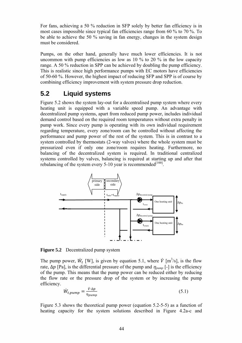
44

For fans, achieving a 50 % reduction in SFP solely by better fan efficiency is in most cases impossible since typical fan efficiencies range from 60 % to 70 %. To be able to achieve the 50 % saving in fan energy, changes in the system design must be considered. Pumps, on the other hand, generally have much lower efficiencies. It is not uncommon with pump efficiencies as low as 10 % to 20 % in the low capacity range. A 50 % reduction in SPP can be achieved by doubling the pump efficiency. This is realistic since high performance pumps with EC motors have efficiencies of 50-60 %. However, the highest impact of reducing SFP and SPP is of course by combining efficiency improvement with system pressure drop reduction.

5.2 Liquid systems Figure 5.2 shows the system lay-out for a decentralised pump system where every heating unit is equipped with a variable speed pump. An advantage with decentralized pump systems, apart from reduced pump power, includes individual demand control based on the required room temperatures without extra penalty in pump work. Since every pump is operating with its own individual requirement regarding temperature, every zone/room can be controlled without affecting the performance and pump power of the rest of the system. This is in contrast to a system controlled by thermostats (2-way valves) where the whole system must be pressurized even if only one zone/room requires heating. Furthermore, no balancing of the decentralized system is required. In traditional centralized systems controlled by valves, balancing is required at starting up and after that rebalancing of the system every 5-10 year is recommended[100].

Figure 5.2 Decentralized pump system

The pump power, [W], is given by equation 5.1, where [m3/s], is the flow rate, ∆ [Pa], is the differential pressure of the pump and pump [-] is the efficiency of the pump. This means that the pump power can be reduced either by reducing the flow rate or the pressure drop of the system or by increasing the pump efficiency.

,·∆

(5.1)

Figure 5.3 shows the theoretical pump power (equation 5.2-5-5) as a function of heating capacity for the system solutions described in Figure 4.2a-c and

Δphu

Δpdecentral pump

treturn

One heating unit

Δpdecentral pump

treturn

tsupply

One heating unit

tinlet=tsupply

Δphu

secondary side

primary side

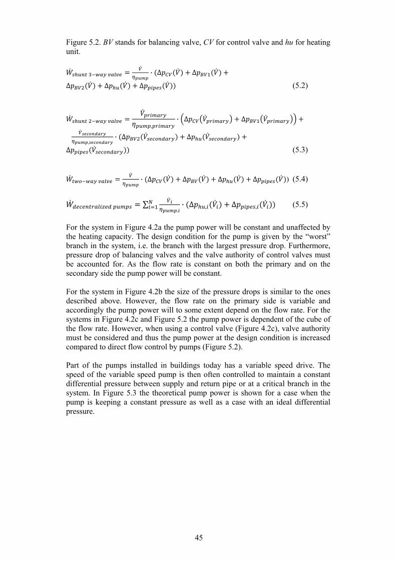
45

Figure 5.2. BV stands for balancing valve, CV for control valve and hu for heating unit.

· ∆ ∆

∆ ∆ ∆ (5.2)

,

· ∆ ∆

,

· ∆ ∆

∆ (5.3)

· ∆ ∆ ∆ ∆ ) (5.4)

∑,

· ∆ , ∆ , (5.5)

For the system in Figure 4.2a the pump power will be constant and unaffected by the heating capacity. The design condition for the pump is given by the “worst” branch in the system, i.e. the branch with the largest pressure drop. Furthermore, pressure drop of balancing valves and the valve authority of control valves must be accounted for. As the flow rate is constant on both the primary and on the secondary side the pump power will be constant. For the system in Figure 4.2b the size of the pressure drops is similar to the ones described above. However, the flow rate on the primary side is variable and accordingly the pump power will to some extent depend on the flow rate. For the systems in Figure 4.2c and Figure 5.2 the pump power is dependent of the cube of the flow rate. However, when using a control valve (Figure 4.2c), valve authority must be considered and thus the pump power at the design condition is increased compared to direct flow control by pumps (Figure 5.2). Part of the pumps installed in buildings today has a variable speed drive. The speed of the variable speed pump is then often controlled to maintain a constant differential pressure between supply and return pipe or at a critical branch in the system. In Figure 5.3 the theoretical pump power is shown for a case when the pump is keeping a constant pressure as well as a case with an ideal differential pressure.

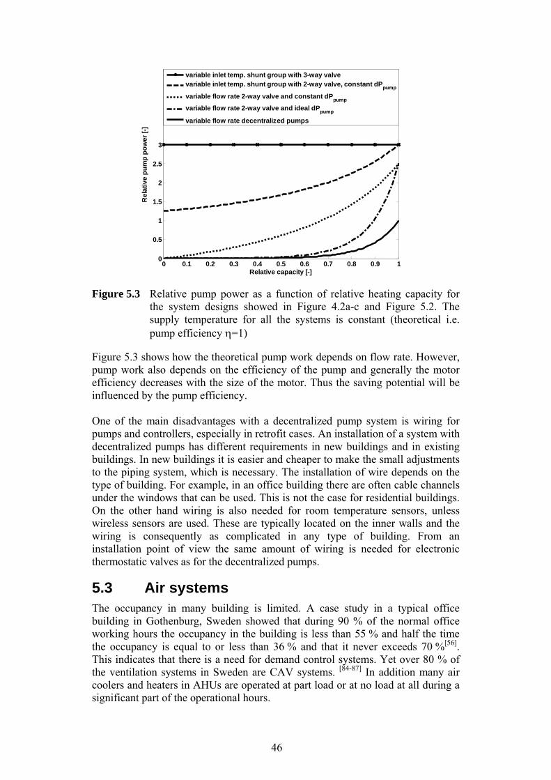
46

Figure 5.3 Relative pump power as a function of relative heating capacity for

the system designs showed in Figure 4.2a-c and Figure 5.2. The supply temperature for all the systems is constant (theoretical i.e. pump efficiency =1)

Figure 5.3 shows how the theoretical pump work depends on flow rate. However, pump work also depends on the efficiency of the pump and generally the motor efficiency decreases with the size of the motor. Thus the saving potential will be influenced by the pump efficiency. One of the main disadvantages with a decentralized pump system is wiring for pumps and controllers, especially in retrofit cases. An installation of a system with decentralized pumps has different requirements in new buildings and in existing buildings. In new buildings it is easier and cheaper to make the small adjustments to the piping system, which is necessary. The installation of wire depends on the type of building. For example, in an office building there are often cable channels under the windows that can be used. This is not the case for residential buildings. On the other hand wiring is also needed for room temperature sensors, unless wireless sensors are used. These are typically located on the inner walls and the wiring is consequently as complicated in any type of building. From an installation point of view the same amount of wiring is needed for electronic thermostatic valves as for the decentralized pumps.

5.3 Air systems The occupancy in many building is limited. A case study in a typical office building in Gothenburg, Sweden showed that during 90 % of the normal office working hours the occupancy in the building is less than 55 % and half the time the occupancy is equal to or less than 36 % and that it never exceeds 70 %[56]. This indicates that there is a need for demand control systems. Yet over 80 % of the ventilation systems in Sweden are CAV systems. [84-87] In addition many air coolers and heaters in AHUs are operated at part load or at no load at all during a significant part of the operational hours.

0 0.1 0.2 0.3 0.4 0.5 0.6 0.7 0.8 0.9 10

0.5

1

1.5

2

2.5

3

Relative capacity [-]

Re

lati

ve

pu

mp

po

we

r [-

]

variable inlet temp. shunt group with 3-way valvevariable inlet temp. shunt group with 2-way valve, constant dP

pump

variable flow rate 2-way valve and constant dPpump

variable flow rate 2-way valve and ideal dPpump

variable flow rate decentralized pumps

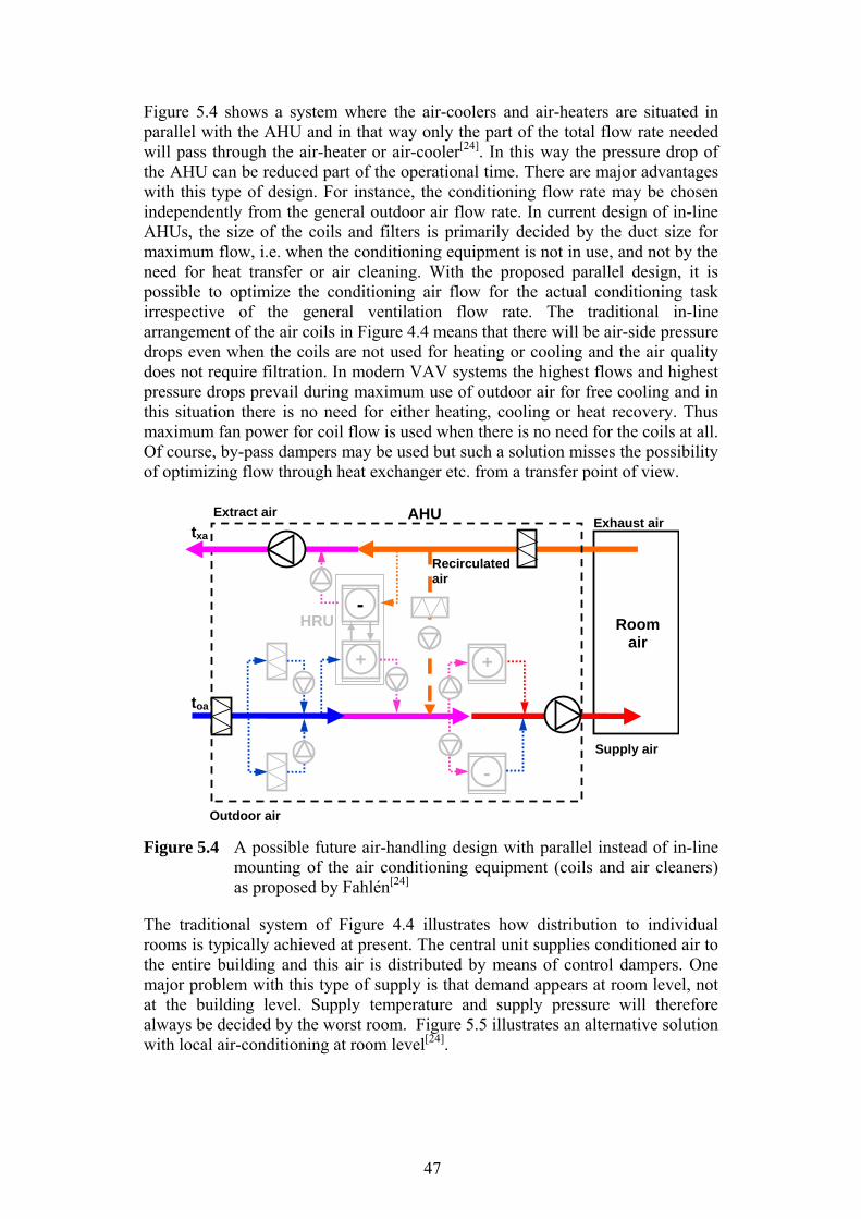
47

Figure 5.4 shows a system where the air-coolers and air-heaters are situated in parallel with the AHU and in that way only the part of the total flow rate needed will pass through the air-heater or air-cooler[24]. In this way the pressure drop of the AHU can be reduced part of the operational time. There are major advantages with this type of design. For instance, the conditioning flow rate may be chosen independently from the general outdoor air flow rate. In current design of in-line AHUs, the size of the coils and filters is primarily decided by the duct size for maximum flow, i.e. when the conditioning equipment is not in use, and not by the need for heat transfer or air cleaning. With the proposed parallel design, it is possible to optimize the conditioning air flow for the actual conditioning task irrespective of the general ventilation flow rate. The traditional in-line arrangement of the air coils in Figure 4.4 means that there will be air-side pressure drops even when the coils are not used for heating or cooling and the air quality does not require filtration. In modern VAV systems the highest flows and highest pressure drops prevail during maximum use of outdoor air for free cooling and in this situation there is no need for either heating, cooling or heat recovery. Thus maximum fan power for coil flow is used when there is no need for the coils at all. Of course, by-pass dampers may be used but such a solution misses the possibility of optimizing flow through heat exchanger etc. from a transfer point of view.

 

Figure 5.4 A possible future air-handling design with parallel instead of in-line mounting of the air conditioning equipment (coils and air cleaners) as proposed by Fahlén[24]

The traditional system of Figure 4.4 illustrates how distribution to individual rooms is typically achieved at present. The central unit supplies conditioned air to the entire building and this air is distributed by means of control dampers. One major problem with this type of supply is that demand appears at room level, not at the building level. Supply temperature and supply pressure will therefore always be decided by the worst room. Figure 5.5 illustrates an alternative solution with local air-conditioning at room level[24].

Outdoor air

toa

txa

+

-

+

-

Extract air Exhaust air

Supply air

Room air

HRU

Recirculated air

AHU

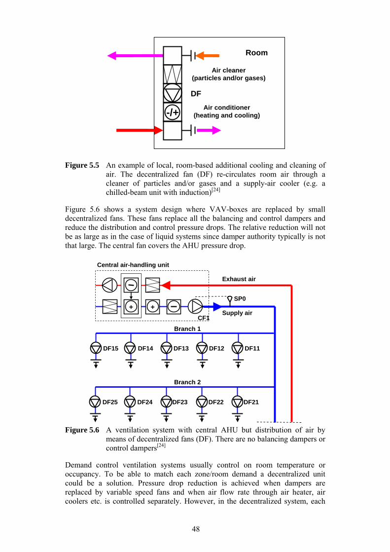
48

Figure 5.5 An example of local, room-based additional cooling and cleaning of air. The decentralized fan (DF) re-circulates room air through a cleaner of particles and/or gases and a supply-air cooler (e.g. a chilled-beam unit with induction)[24]

Figure 5.6 shows a system design where VAV-boxes are replaced by small decentralized fans. These fans replace all the balancing and control dampers and reduce the distribution and control pressure drops. The relative reduction will not be as large as in the case of liquid systems since damper authority typically is not that large. The central fan covers the AHU pressure drop.

Figure 5.6 A ventilation system with central AHU but distribution of air by

means of decentralized fans (DF). There are no balancing dampers or control dampers[24]

Demand control ventilation systems usually control on room temperature or occupancy. To be able to match each zone/room demand a decentralized unit could be a solution. Pressure drop reduction is achieved when dampers are replaced by variable speed fans and when air flow rate through air heater, air coolers etc. is controlled separately. However, in the decentralized system, each

-/+

Room

DF

Air cleaner(particles and/or gases)

Air conditioner(heating and cooling)

Exhaust air

Central air-handling unit

Supply air

Branch 1

Branch 2

DF11 DF12 DF13 DF14 DF15

DF21 DF22 DF23 DF24 DF25

SP0

+ +

CF1

49

zone/room needs a fan and typically the fan efficiency decreases with decreasing size. Important when considering decentralized fan systems in general possible noise aspects must be considered.

5.4 Requirements on future components and control systems

In the decentralized systems described above the system pressure drop is reduced substantially when the flow rate is controlled by variable speed pumps and fans and removing controlling devices as control valves and dampers. However, as smaller pumps and fans usually have lower efficiency than larger pumps and fans, efficiency needs to be considered. The efficiency of variable speed pumps and fans can be divided into the following parts:

‐ Hydraulic efficiency ‐ Motor efficiency ‐ Frequency converter efficiency

To determine the total efficiency it is necessary to calculate the load characteristics, i.e. the pump/fan operating points. Using pump/fan load characteristics it is possible to size the drive with an appropriate motor and frequency converter. In Figure 5.7 the characteristics for a pump is shown. Also included in the figure are two system characteristics, one with a constant differential pressure and one where the differential pressure is proportional to the square of the speed (the two system characteristics have the same nominal pressure drop and nominal flow rate). The system with the constant differential pressure is comparable to a pump operated with a fixed differential pressure, which is commonly how variable speed pumps are operated. The system with variable differential pressure is comparable with a variable speed pump which is providing the ideal differential pressure for every flow rate. The shape of the pump characteristic is given by manufacturers’ data. Equations 5.6 to 5.9 (affinity laws) are used for recalculating the pump characteristics for variable pump speeds.

·

· (5.6)

·

· (5.7)

·

· (5.8)

n is the pump speed and D is the pump diameter.

50

Figure 5.7 Relative differential pressure as a function of relative flow rate for a

number of pump speeds. Two system characteristics are included, one for constant differential pressure and one where the differential pressure is dependent of the square of the flow rate

Figure 5.8 shows the relative efficiency as a function of relative flow rate based on the affinity laws for a number of pump speeds. At fixed speed the efficiency is highly dependent of flow rate. However, when changing speed the efficiency is constant.

Figure 5.8 Relative efficiency as a function of relative flow rate for a number of

pump speeds

0 0.2 0.4 0.6 0.8 10

0.2

0.4

0.6

0.8

1

Relative flow rate [-]

Re

lati

ve

dif

fere

nti

al p

res

su

re [

-]

System curve - variable dP

system curve -constant dP

Decreasing speed from 100 % to 25 %

0 0.2 0.4 0.6 0.8 10

0.2

0.4

0.6

0.8

1

1.2

Re

lati

ve

eff

icie

nc

y [

-]

Relative flow rate [-]

decreasing speed from 100 % to 25 %

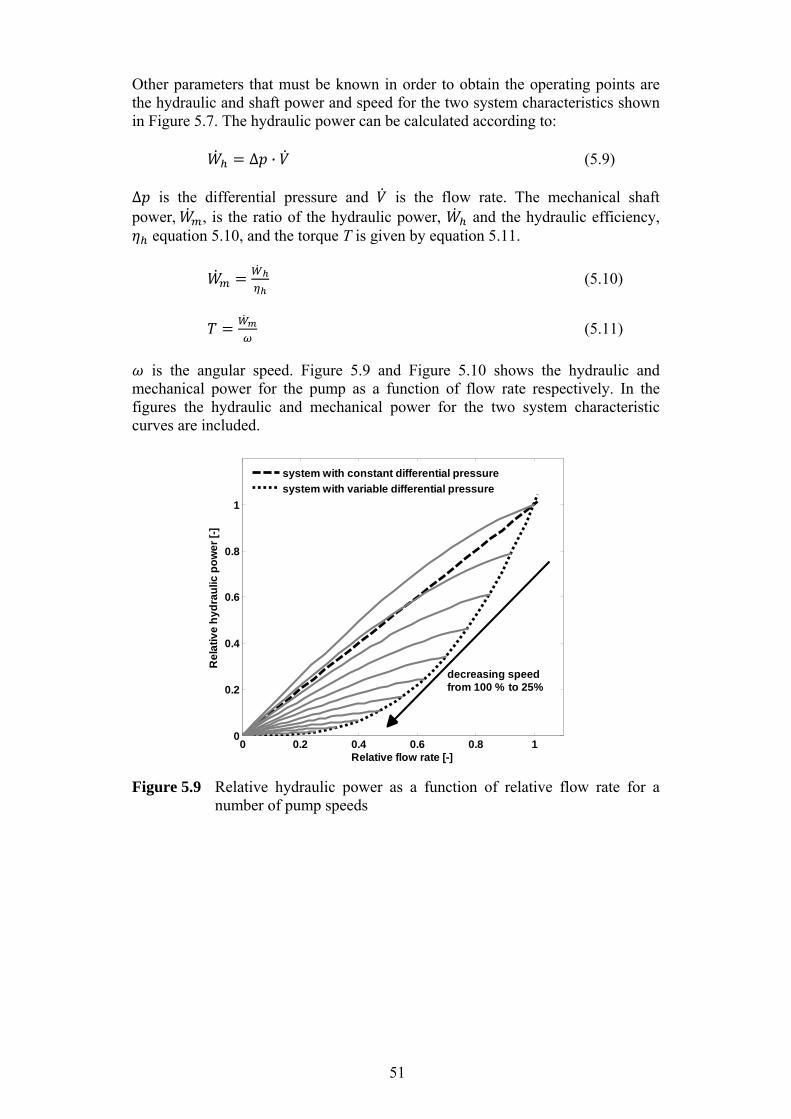
51

Other parameters that must be known in order to obtain the operating points are the hydraulic and shaft power and speed for the two system characteristics shown in Figure 5.7. The hydraulic power can be calculated according to: ∆ · (5.9) Δ is the differential pressure and is the flow rate. The mechanical shaft power, , is the ratio of the hydraulic power, and the hydraulic efficiency,

equation 5.10, and the torque T is given by equation 5.11.

(5.10)

(5.11)

is the angular speed. Figure 5.9 and Figure 5.10 shows the hydraulic and

mechanical power for the pump as a function of flow rate respectively. In the figures the hydraulic and mechanical power for the two system characteristic curves are included.

Figure 5.9 Relative hydraulic power as a function of relative flow rate for a

number of pump speeds

0 0.2 0.4 0.6 0.8 10

0.2

0.4

0.6

0.8

1

Relative flow rate [-]

Re

lati

ve

hy

dra

ulic

po

we

r [-

]

system with constant differential pressure

system with variable differential pressure

decreasing speed from 100 % to 25%

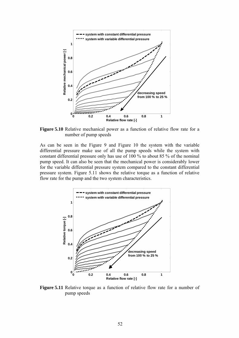
52

Figure 5.10 Relative mechanical power as a function of relative flow rate for a

number of pump speeds

As can be seen in the Figure 9 and Figure 10 the system with the variable differential pressure make use of all the pump speeds while the system with constant differential pressure only has use of 100 % to about 85 % of the nominal pump speed. It can also be seen that the mechanical power is considerably lower for the variable differential pressure system compared to the constant differential pressure system. Figure 5.11 shows the relative torque as a function of relative flow rate for the pump and the two system characteristics.

Figure 5.11 Relative torque as a function of relative flow rate for a number of

pump speeds

0 0.2 0.4 0.6 0.8 10

0.2

0.4

0.6

0.8

1

Relative flow rate [-]

Re

lativ

e m

ech

anic

al p

ow

er

[-]

system with constant differential pressure

system with variable differential pressure

decreasing speed from 100 % to 25 %

0 0.2 0.4 0.6 0.8 10

0.2

0.4

0.6

0.8

1

Relative flow rate [-]

Re

lativ

e t

orq

ue

[-]

system with constant differential pressure

system with variable differential pressure

decreasing speedfrom 100 % to 25 %

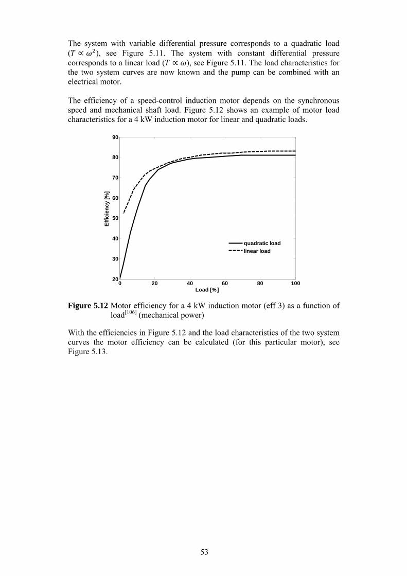
53

The system with variable differential pressure corresponds to a quadratic load ( ), see Figure 5.11. The system with constant differential pressure corresponds to a linear load ( ), see Figure 5.11. The load characteristics for the two system curves are now known and the pump can be combined with an electrical motor. The efficiency of a speed-control induction motor depends on the synchronous speed and mechanical shaft load. Figure 5.12 shows an example of motor load characteristics for a 4 kW induction motor for linear and quadratic loads.

Figure 5.12 Motor efficiency for a 4 kW induction motor (eff 3) as a function of

load[106] (mechanical power)

With the efficiencies in Figure 5.12 and the load characteristics of the two system curves the motor efficiency can be calculated (for this particular motor), see Figure 5.13.

0 20 40 60 80 10020

30

40

50

60

70

80

90

Load [%]

Eff

icie

nc

y [

%]

quadratic load

linear load

54

Figure 5.13 The motor efficiency as a function of relative flow rate for the two

system characteristics

The motor efficiency for the system with variable differential pressure falls drastically with reduced flow rate, while the motor efficiency for the system with constant differential pressure keeps within ±3 % for the whole operational range. The efficiency of a frequency converter is fairly constant (about 2 % change) in a wide operational range (about 100 % to 30-40 % of load). However the efficiency of the frequency converter drops for reduced loads. Figure 5.14 shows an example of efficiency of a converter[106].

Figure 5.14 Converter efficiency as a function of load[106]

0 0.2 0.4 0.6 0.8 110

20

30

40

50

60

70

80

90

Relative flow rate [-]

Mo

tor

eff

icie

nc

y [

%]

system curve - constant dP

system curve - variable dP

0 20 40 60 80 1000

10

20

30

40

50

60

70

80

90

100

Load [%]

Co

nve

rte

r e

ffic

ien

cy

[%]

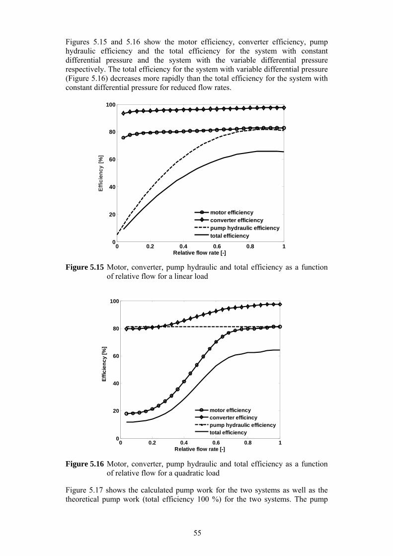
55

Figures 5.15 and 5.16 show the motor efficiency, converter efficiency, pump hydraulic efficiency and the total efficiency for the system with constant differential pressure and the system with the variable differential pressure respectively. The total efficiency for the system with variable differential pressure (Figure 5.16) decreases more rapidly than the total efficiency for the system with constant differential pressure for reduced flow rates.

Figure 5.15 Motor, converter, pump hydraulic and total efficiency as a function

of relative flow for a linear load

Figure 5.16 Motor, converter, pump hydraulic and total efficiency as a function

of relative flow for a quadratic load

Figure 5.17 shows the calculated pump work for the two systems as well as the theoretical pump work (total efficiency 100 %) for the two systems. The pump

0 0.2 0.4 0.6 0.8 10

20

40

60

80

100

Relative flow rate [-]

Eff

icie

nc

y [

%]

motor efficiencyconverter efficiencypump hydraulic efficiencytotal efficiency

0 0.2 0.4 0.6 0.8 10

20

40

60

80

100

Relative flow rate [-]

Eff

icie

nc

y [

%]

motor efficiencyconverter efficincypump hydraulic efficiencytotal efficiency

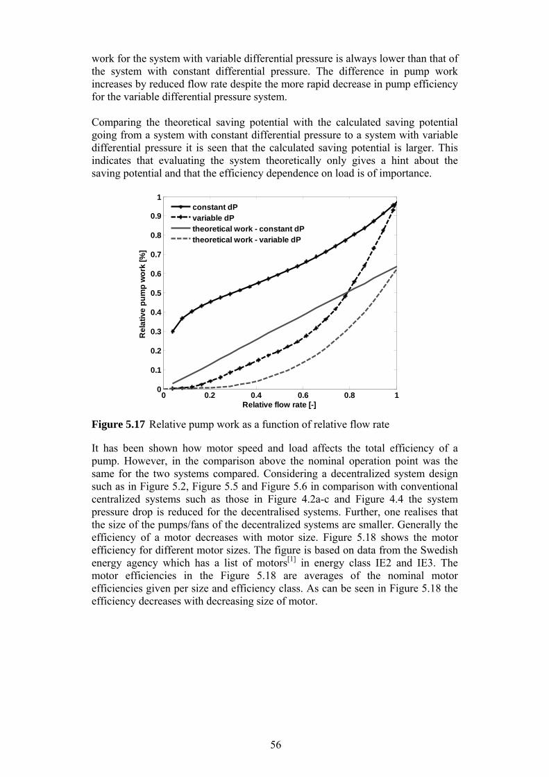
56

work for the system with variable differential pressure is always lower than that of the system with constant differential pressure. The difference in pump work increases by reduced flow rate despite the more rapid decrease in pump efficiency for the variable differential pressure system. Comparing the theoretical saving potential with the calculated saving potential going from a system with constant differential pressure to a system with variable differential pressure it is seen that the calculated saving potential is larger. This indicates that evaluating the system theoretically only gives a hint about the saving potential and that the efficiency dependence on load is of importance.

Figure 5.17 Relative pump work as a function of relative flow rate

It has been shown how motor speed and load affects the total efficiency of a pump. However, in the comparison above the nominal operation point was the same for the two systems compared. Considering a decentralized system design such as in Figure 5.2, Figure 5.5 and Figure 5.6 in comparison with conventional centralized systems such as those in Figure 4.2a-c and Figure 4.4 the system pressure drop is reduced for the decentralised systems. Further, one realises that the size of the pumps/fans of the decentralized systems are smaller. Generally the efficiency of a motor decreases with motor size. Figure 5.18 shows the motor efficiency for different motor sizes. The figure is based on data from the Swedish energy agency which has a list of motors[1] in energy class IE2 and IE3. The motor efficiencies in the Figure 5.18 are averages of the nominal motor efficiencies given per size and efficiency class. As can be seen in Figure 5.18 the efficiency decreases with decreasing size of motor.

0 0.2 0.4 0.6 0.8 10

0.1

0.2

0.3

0.4

0.5

0.6

0.7

0.8

0.9

1

Relative flow rate [-]

Re

lati

ve

pu

mp

wo

rk [

%]

constant dPvariable dPtheoretical work - constant dPtheoretical work - variable dP

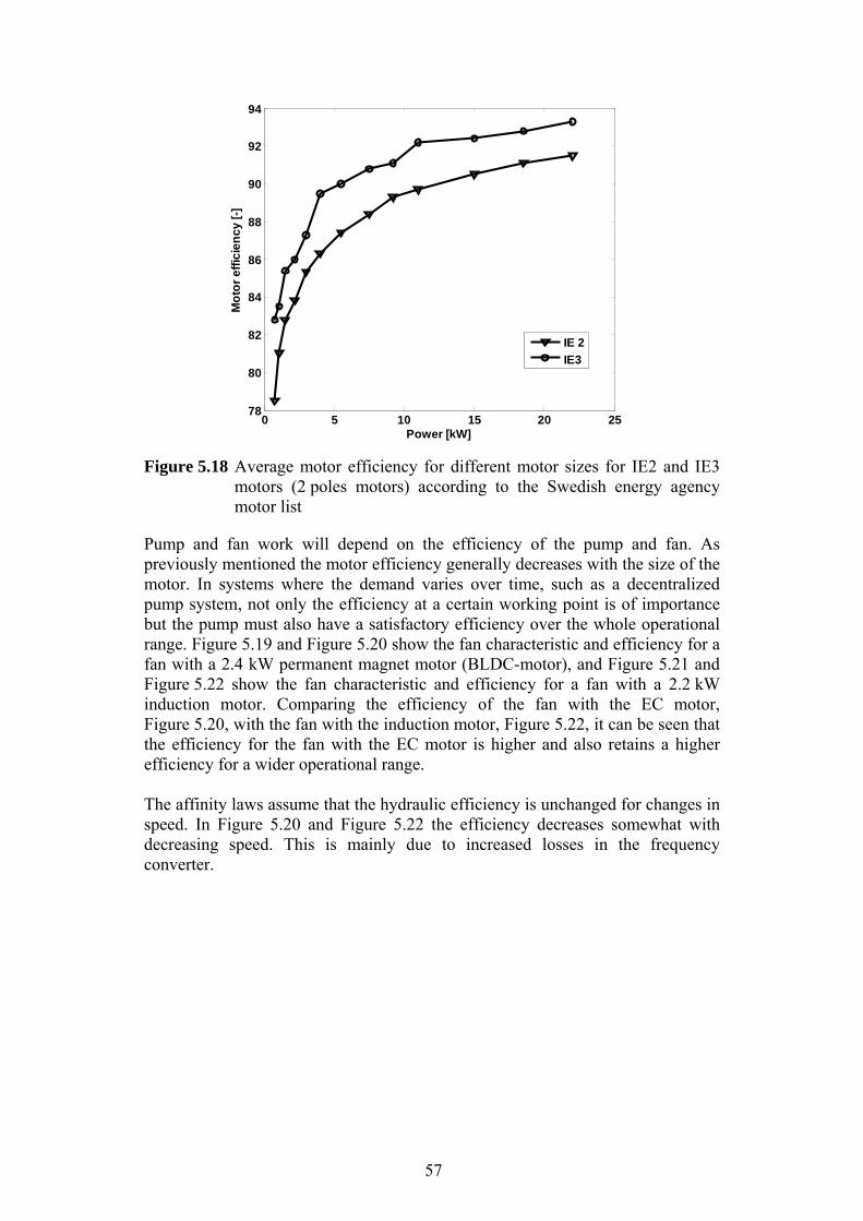
57

Figure 5.18 Average motor efficiency for different motor sizes for IE2 and IE3

motors (2 poles motors) according to the Swedish energy agency motor list

Pump and fan work will depend on the efficiency of the pump and fan. As previously mentioned the motor efficiency generally decreases with the size of the motor. In systems where the demand varies over time, such as a decentralized pump system, not only the efficiency at a certain working point is of importance but the pump must also have a satisfactory efficiency over the whole operational range. Figure 5.19 and Figure 5.20 show the fan characteristic and efficiency for a fan with a 2.4 kW permanent magnet motor (BLDC-motor), and Figure 5.21 and Figure 5.22 show the fan characteristic and efficiency for a fan with a 2.2 kW induction motor. Comparing the efficiency of the fan with the EC motor, Figure 5.20, with the fan with the induction motor, Figure 5.22, it can be seen that the efficiency for the fan with the EC motor is higher and also retains a higher efficiency for a wider operational range. The affinity laws assume that the hydraulic efficiency is unchanged for changes in speed. In Figure 5.20 and Figure 5.22 the efficiency decreases somewhat with decreasing speed. This is mainly due to increased losses in the frequency converter.

0 5 10 15 20 2578

80

82

84

86

88

90

92

94

Mo

tor

eff

icie

ncy

[-]

Power [kW]

IE 2

IE3

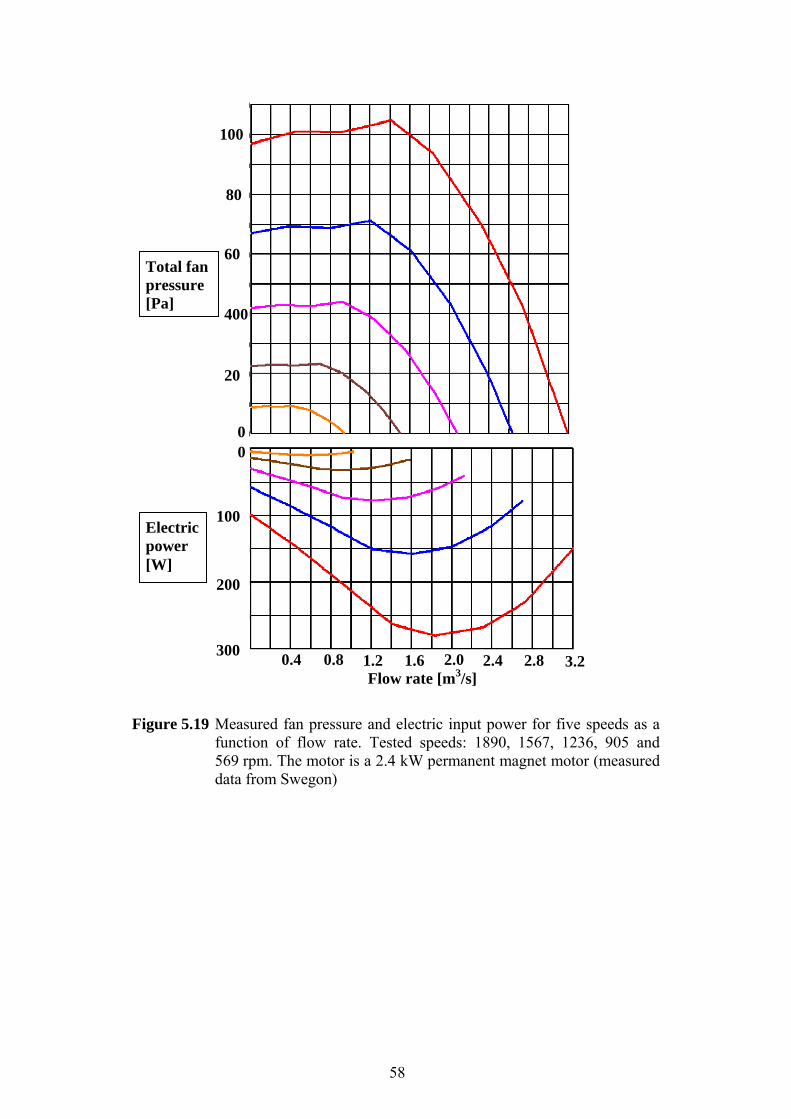
58

Figure 5.19 Measured fan pressure and electric input power for five speeds as a

function of flow rate. Tested speeds: 1890, 1567, 1236, 905 and 569 rpm. The motor is a 2.4 kW permanent magnet motor (measured data from Swegon)

100

80

60

400

20

0

Total fan pressure [Pa]

0

200

100

3000.8 0.4 3.2 2.0 1.6 1.2 2.8 2.4

Electric power [W]

Flow rate [m3/s]

59

Figure 5.20 The fan efficiency as a function of flow rate for the fan in Figure

5.19. Tested speeds: 1890, 1567, 1236, 905 and 569 rpm. (measured data from Swegon)

3.2 2.8

Flow rate [m3/s]

0.8 0.4 2.0 1.6 1.2 2.4 0

10

30

40

20

50

60

Total fan efficiency [%]

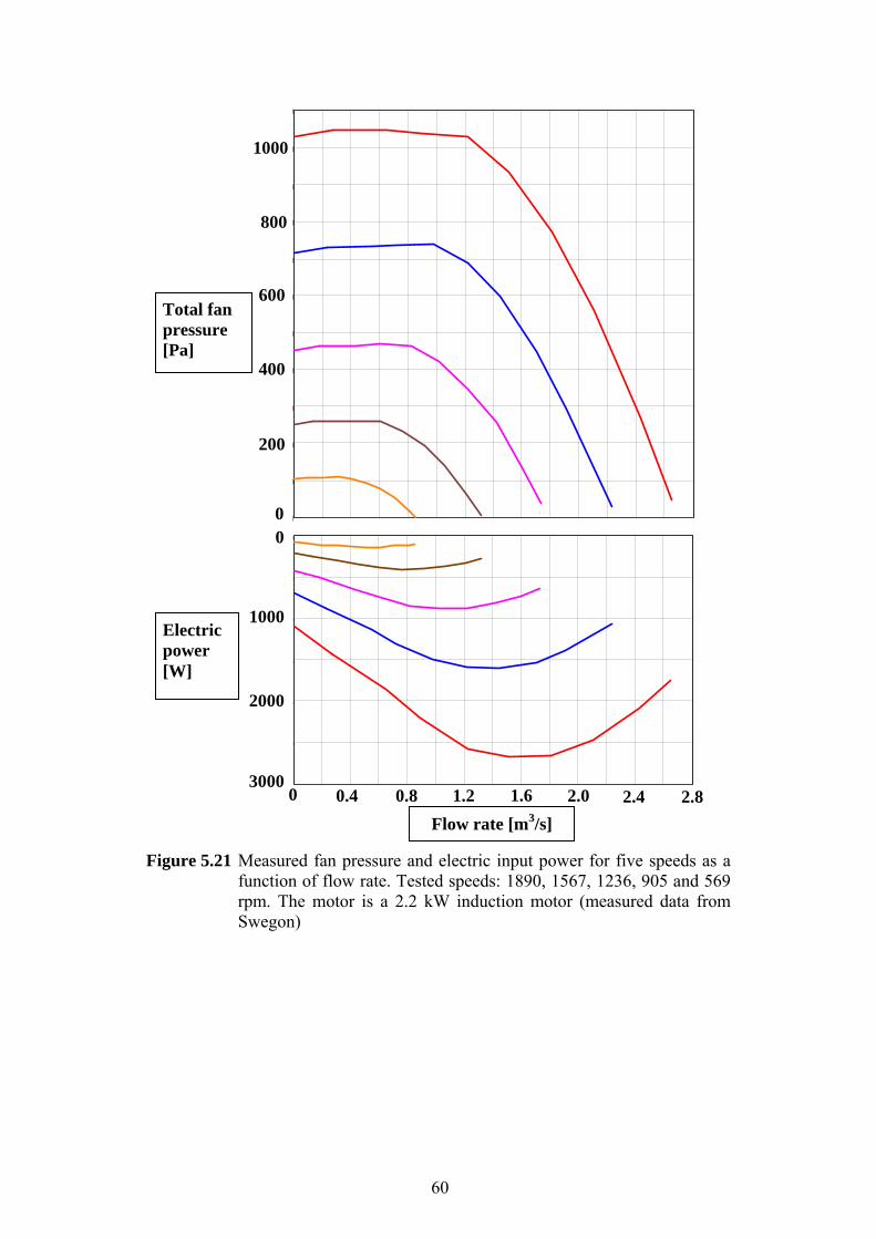
60

Figure 5.21 Measured fan pressure and electric input power for five speeds as a

function of flow rate. Tested speeds: 1890, 1567, 1236, 905 and 569 rpm. The motor is a 2.2 kW induction motor (measured data from Swegon)

0

100

200

300

400

500

600

700

800

900

1000

1100

To

tal

pres

sure

ris

e, P

a

0 0.2 0.4 0.6 0.8 1 1.2 1.4 1.6 1.8 2 2.2 2.4 2.6 2.8

0

2500

2000

1500

1000

500

0

Air flow, m³/s

Ele

ctri

cal p

ower

, W

1000

800

600

400

200

0

Total fan pressure [Pa]

0

2000

1000

3000 0.8 0.4 2.0 1.6 1.2 2.8 2.4

Electric power [W]

Flow rate [m3/s]

0

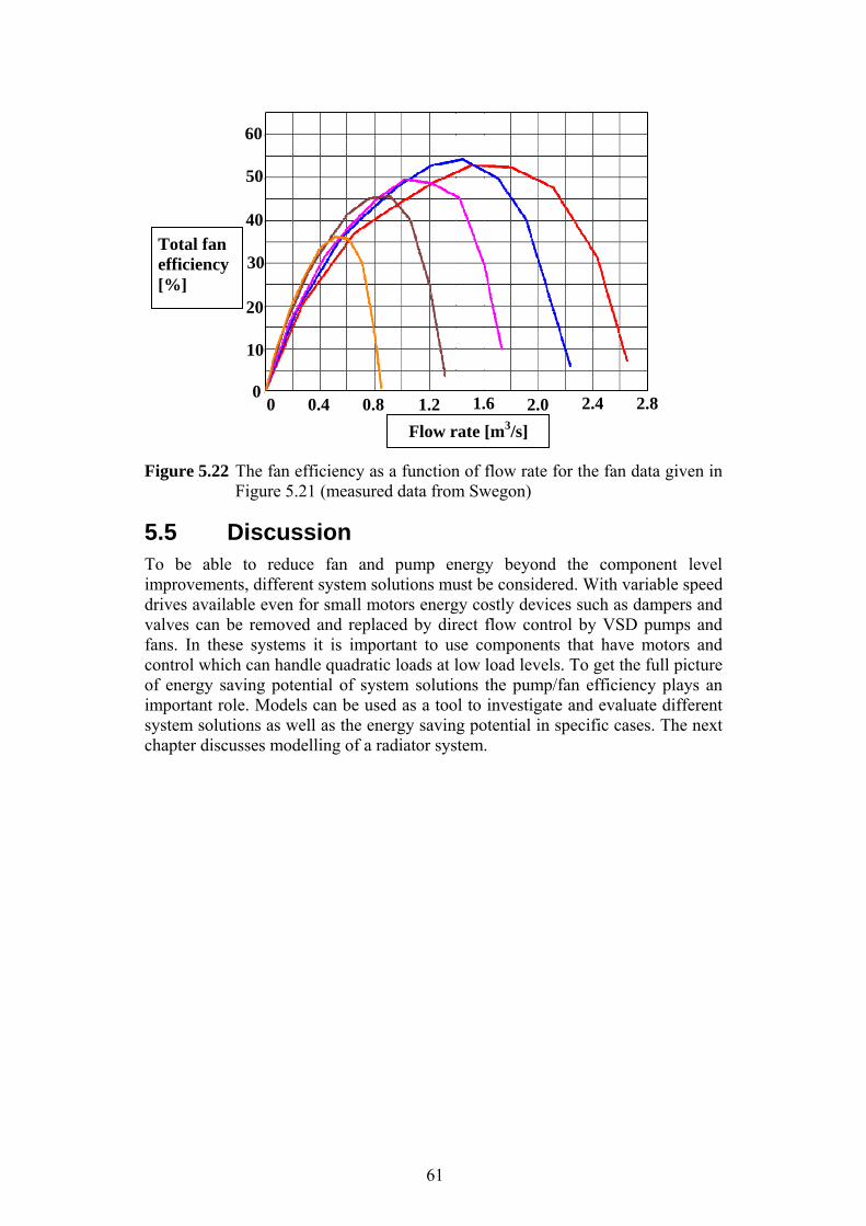
61

Figure 5.22 The fan efficiency as a function of flow rate for the fan data given in

Figure 5.21 (measured data from Swegon)

5.5 Discussion To be able to reduce fan and pump energy beyond the component level improvements, different system solutions must be considered. With variable speed drives available even for small motors energy costly devices such as dampers and valves can be removed and replaced by direct flow control by VSD pumps and fans. In these systems it is important to use components that have motors and control which can handle quadratic loads at low load levels. To get the full picture of energy saving potential of system solutions the pump/fan efficiency plays an important role. Models can be used as a tool to investigate and evaluate different system solutions as well as the energy saving potential in specific cases. The next chapter discusses modelling of a radiator system.

2.8

Flow rate [m3/s]

0.8 0.4 2.0 1.6 1.2 2.4 0

10

30

40

20

50

60

Total fan efficiency [%]

0

62

63

6 System simulation example Measurement of a radiator system in an office building provides a base for a model. The model is a simplified room model adapted to fit the temperature variations in an office room. Although its simplicity it will fulfil its purpose which is to obtain a way for evaluations of pump, and heating energies for radiator systems solutions.

6.1 Model and model validation The model validation measurement period chosen is a four week period during December 2010 when the outdoor temperature is relatively low and radiation from the sun is assumed to be more or less neglected. The windows of the office building are facing east and a neighbouring house is shading the windows. The system on which the measurements are conducted is a decentralized radiator system where every radiator is equipped with a small pump, Figure 6.1. The system is located on the top floor of the building. Table 6.1 gives an overview of the measured parameters in the system. The measurements were conducted for all the rooms and radiators but the model is validated and calculated for only one of the office rooms. During the measurements temperature set-back was used for non-working hours. During working hours Monday to Friday 7 am to 6 pm the set room temperature was 21.5 °C and for non-working hours and weekends the set room temperature was 16 °C. Figure 6.2 shows the duration diagram for the outdoor temperature during the measurement period.

Figure 6.1 System design of measured pump system

secondary side

primary side

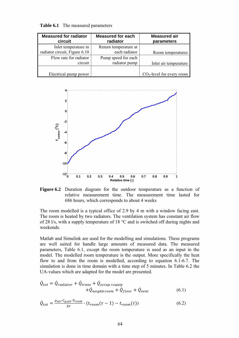
64

Table 6.1 The measured parameters

Measured for radiator circuit

Measured for each radiator

Measured air parameters

Inlet temperature in radiator circuit, Figure 6.10

Return temperature at each radiator

Room temperatures

Flow rate for radiator circuit

Pump speed for each radiator pump

Inlet air temperature

Electrical pump power

CO2-level for every room

Figure 6.2 Duration diagram for the outdoor temperature as a function of

relative measurement time. The measurement time lasted for 686 hours, which corresponds to about 4 weeks

The room modelled is a typical office of 2.9 by 4 m with a window facing east. The room is heated by two radiators. The ventilation system has constant air flow of 28 l/s, with a supply temperature of 18 °C and is switched off during nights and weekends. Matlab and Simulink are used for the modelling and simulations. These programs are well suited for handle large amounts of measured data. The measured parameters, Table 6.1, except the room temperature is used as an input in the model. The modelled room temperature is the output. More specifically the heat flow to and from the room is modelled, according to equation 6.1-6.7. The simulation is done in time domain with a time step of 5 minutes. In Table 6.2 the UA-values which are adapted for the model are presented.

. . (6.1)

· , ·

∆· 1 ) (6.2)

0 0.1 0.2 0.3 0.4 0.5 0.6 0.7 0.8 0.9 1-12

-10

-8

-6

-4

-2

0

2

4

Relative time [-]

To

utd

oo

r [oC

]

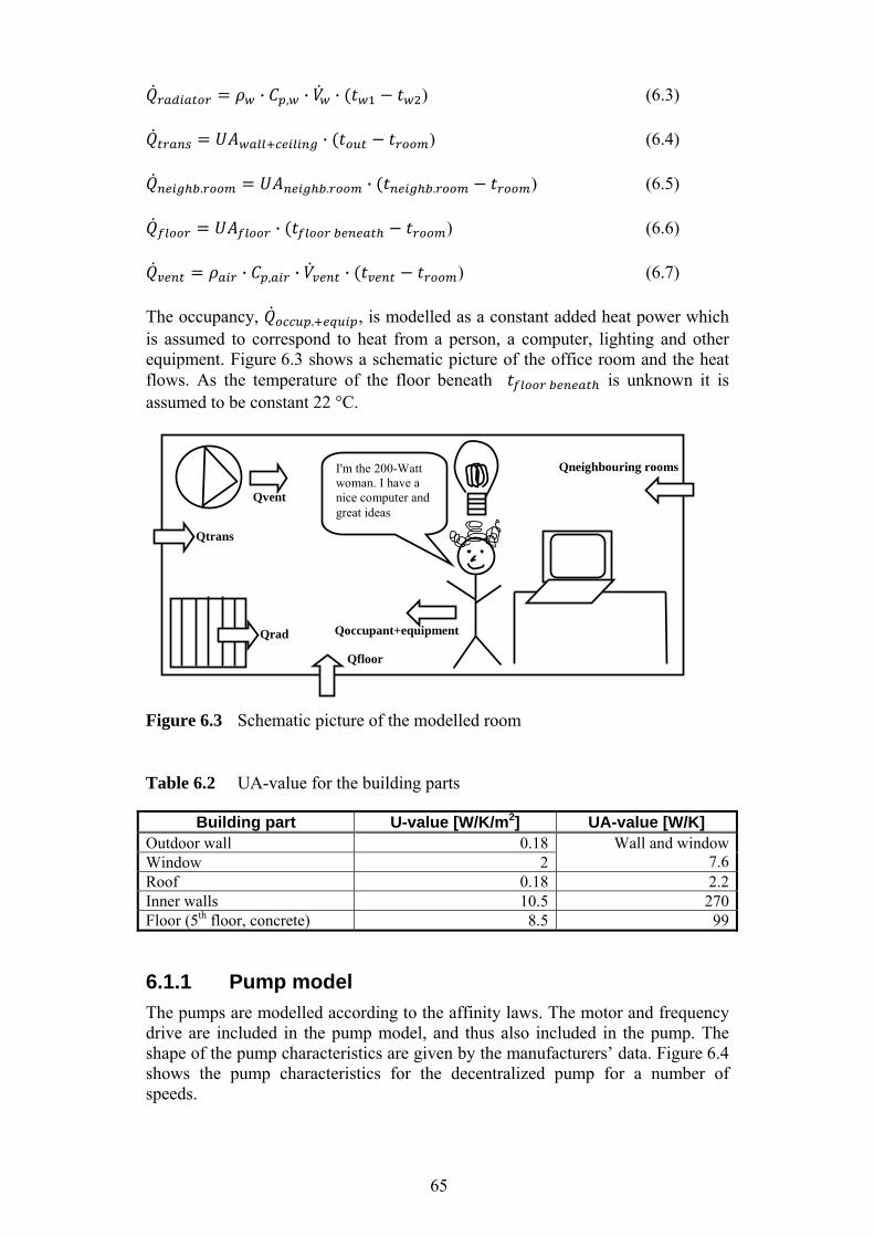
65

· , · · ) (6.3)

· ) (6.4)

. . · . ) (6.5)

· ) (6.6)

· , · · ) (6.7) The occupancy, . , is modelled as a constant added heat power which is assumed to correspond to heat from a person, a computer, lighting and other equipment. Figure 6.3 shows a schematic picture of the office room and the heat flows. As the temperature of the floor beneath is unknown it is assumed to be constant 22 °C.

Qrad

Qfloor

I'm the 200-Watt woman. I have a nice computer and great ideas

Qoccupant+equipment

Qneighbouring rooms

Qvent

Qtrans

Figure 6.3 Schematic picture of the modelled room

Table 6.2 UA-value for the building parts

Building part U-value [W/K/m2] UA-value [W/K] Outdoor wall 0.18 Wall and window

7.6Window 2Roof 0.18 2.2Inner walls 10.5 270Floor (5th floor, concrete) 8.5 99

6.1.1 Pump model

The pumps are modelled according to the affinity laws. The motor and frequency drive are included in the pump model, and thus also included in the pump. The shape of the pump characteristics are given by the manufacturers’ data. Figure 6.4 shows the pump characteristics for the decentralized pump for a number of speeds.

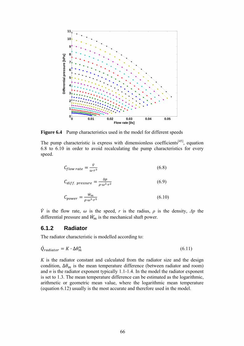
66

Figure 6.4 Pump characteristics used in the model for different speeds

The pump characteristic is express with dimensionless coefficients[45], equation 6.8 to 6.10 in order to avoid recalculating the pump characteristics for every speed.

· (6.8)

. ∆

· · (6.9)

· ·

(6.10)

is the flow rate, is the speed, r is the radius, ρ is the density, Δp the

differential pressure and is the mechanical shaft power.

6.1.2 Radiator

The radiator characteristic is modelled according to:

· ∆ (6.11) K is the radiator constant and calculated from the radiator size and the design condition, ∆ is the mean temperature difference (between radiator and room) and n is the radiator exponent typically 1.1-1.4. In the model the radiator exponent is set to 1.3. The mean temperature difference can be estimated as the logarithmic, arithmetic or geometric mean value, where the logarithmic mean temperature (equation 6.12) usually is the most accurate and therefore used in the model.

0 0.01 0.02 0.03 0.04 0.050

1

2

3

4

5

6

7

8

9

10

11

Flow rate [l/s]

Dif

fere

nti

al p

res

su

re [

kP

a]

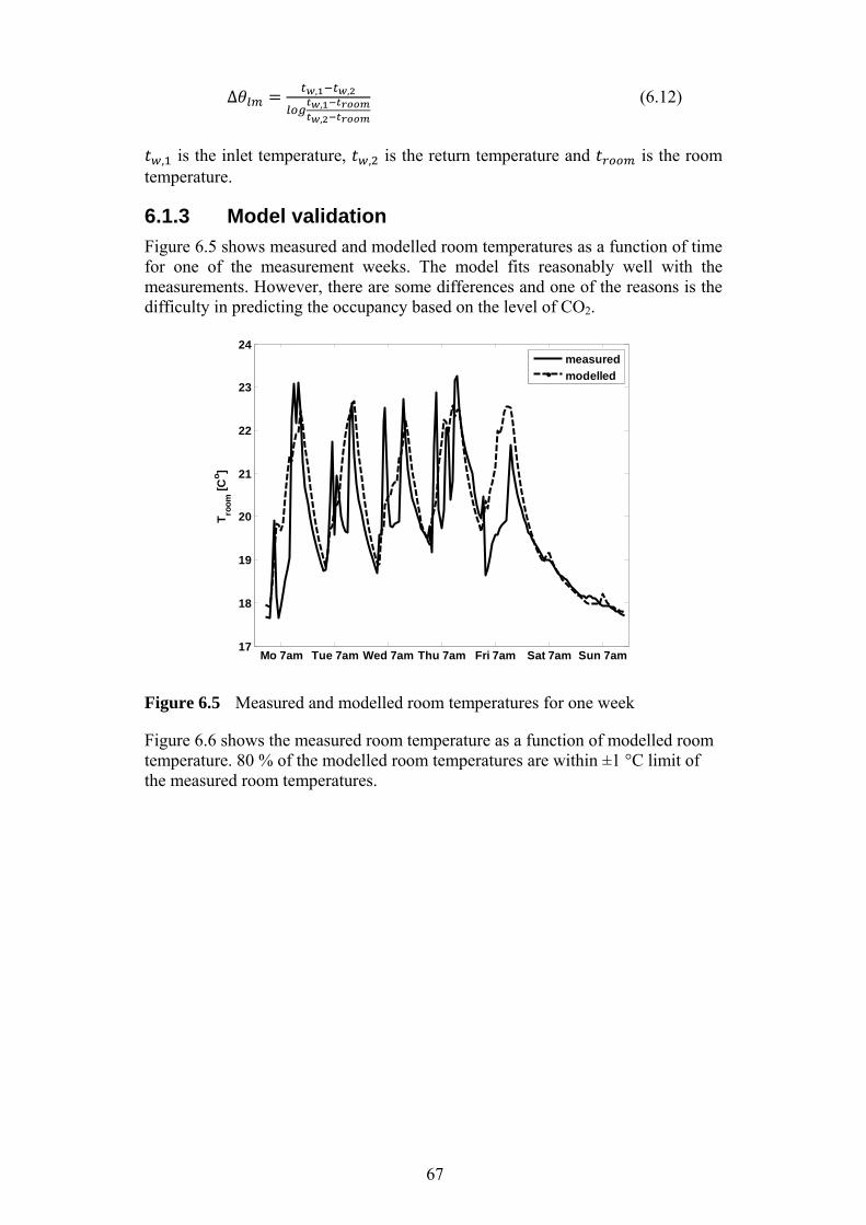
67

∆ , ,,,

(6.12)

, is the inlet temperature, , is the return temperature and is the room

temperature.

6.1.3 Model validation

Figure 6.5 shows measured and modelled room temperatures as a function of time for one of the measurement weeks. The model fits reasonably well with the measurements. However, there are some differences and one of the reasons is the difficulty in predicting the occupancy based on the level of CO2.

Figure 6.5 Measured and modelled room temperatures for one week

Figure 6.6 shows the measured room temperature as a function of modelled room temperature. 80 % of the modelled room temperatures are within ±1 °C limit of the measured room temperatures.

Mo 7am Tue 7am Wed 7am Thu 7am Fri 7am Sat 7am Sun 7am17

18

19

20

21

22

23

24

Tro

om

[C

o]

measured

modelled

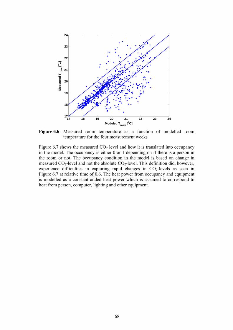
68

Figure 6.6 Measured room temperature as a function of modelled room

temperature for the four measurement weeks

Figure 6.7 shows the measured CO2 level and how it is translated into occupancy in the model. The occupancy is either 0 or 1 depending on if there is a person in the room or not. The occupancy condition in the model is based on change in measured CO2-level and not the absolute CO2-level. This definition did, however, experience difficulties in capturing rapid changes in CO2-levels as seen in Figure 6.7 at relative time of 0.6. The heat power from occupancy and equipment is modelled as a constant added heat power which is assumed to correspond to heat from person, computer, lighting and other equipment.

17 18 19 20 21 22 23 2417

18

19

20

21

22

23

24

Modeled Troom

[oC]

Me

as

ure

d T

roo

m [

oC

]

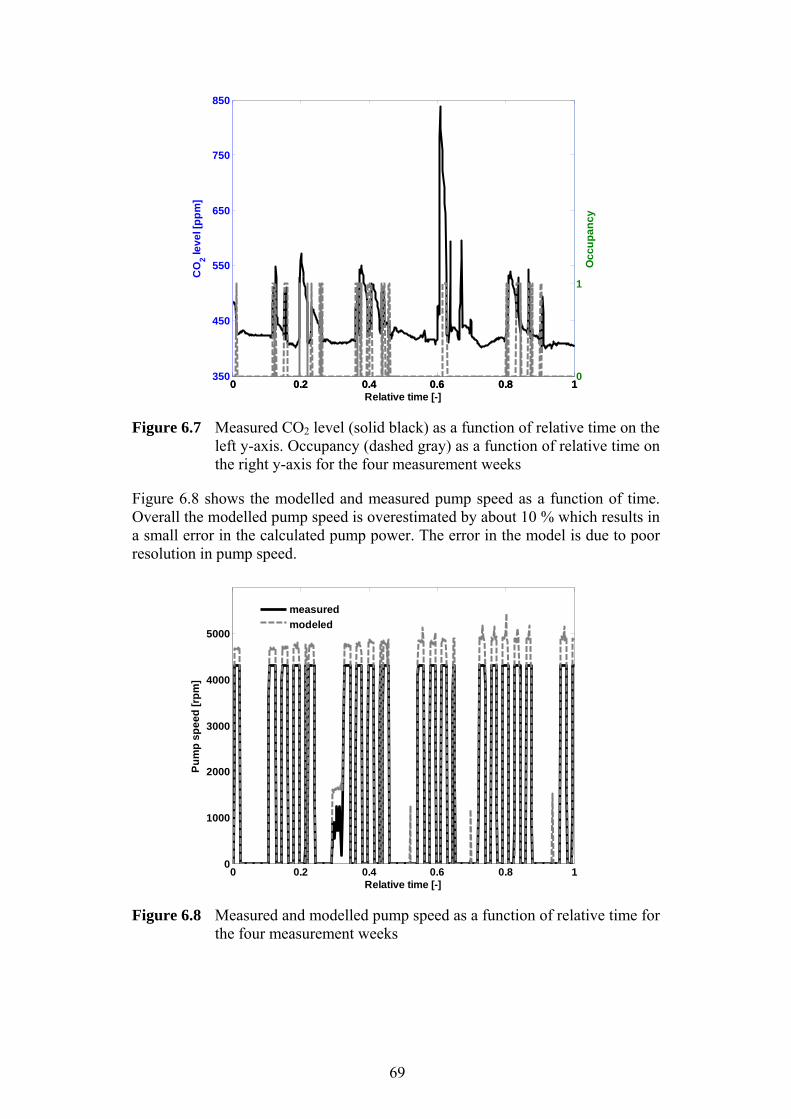
69

Figure 6.7 Measured CO2 level (solid black) as a function of relative time on the

left y-axis. Occupancy (dashed gray) as a function of relative time on the right y-axis for the four measurement weeks

Figure 6.8 shows the modelled and measured pump speed as a function of time. Overall the modelled pump speed is overestimated by about 10 % which results in a small error in the calculated pump power. The error in the model is due to poor resolution in pump speed.

Figure 6.8 Measured and modelled pump speed as a function of relative time for

the four measurement weeks

0 0.2 0.4 0.6 0.8 1350

450

550

650

750

850

CO

2 le

ve

l [p

pm

]

0 0.2 0.4 0.6 0.8 10

1

Relative time [-]

Oc

cu

pa

nc

y

0 0.2 0.4 0.6 0.8 10

1000

2000

3000

4000

5000

Relative time [-]

Pu

mp

sp

ee

d [

rpm

]

measured

modeled

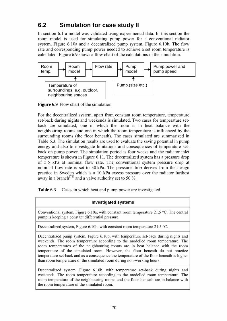
70

6.2 Simulation for case study II In section 6.1 a model was validated using experimental data. In this section the room model is used for simulating pump power for a conventional radiator system, Figure 6.10a and a decentralized pump system, Figure 6.10b. The flow rate and corresponding pump power needed to achieve a set room temperature is calculated. Figure 6.9 shows a flow chart of the calculations in the simulation.

Figure 6.9 Flow chart of the simulation For the decentralized system, apart from constant room temperature, temperature set-back during nights and weekends is simulated. Two cases for temperature set-back are simulated; one in which the room is in heat balance with the neighbouring rooms and one in which the room temperature is influenced by the surrounding rooms (the floor beneath). The cases simulated are summarized in Table 6.3. The simulation results are used to evaluate the saving potential in pump energy and also to investigate limitations and consequences of temperature set-back on pump power. The simulation period is four weeks and the radiator inlet temperature is shown in Figure 6.11. The decentralized system has a pressure drop of 5.5 kPa at nominal flow rate. The conventional system pressure drop at nominal flow rate is set to 30 kPa. The pressure drop derives from the design practice in Sweden which is a 10 kPa excess pressure over the radiator furthest away in a branch[71] and a valve authority set to 50 %.

Table 6.3 Cases in which heat and pump power are investigated

Investigated systems

Conventional system, Figure 6.10a, with constant room temperature 21.5 °C. The central pump is keeping a constant differential pressure.

Decentralized system, Figure 6.10b, with constant room temperature 21.5 °C.

Decentralized pump system, Figure 6.10b, with temperature set-back during nights and weekends. The room temperature according to the modelled room temperature. The room temperatures of the neighbouring rooms are in heat balance with the room temperature of the simulated room. However, the floor beneath do not practice temperature set-back and as a consequence the temperature of the floor beneath is higher than room temperature of the simulated room during non-working hours

Decentralized system, Figure 6.10b, with temperature set-back during nights and weekends. The room temperature according to the modelled room temperature. The room temperature of the neighbouring rooms and the floor beneath are in balance with the room temperature of the simulated room.

Temperature of surroundings, e.g. outdoor, neighbouring spaces

Pump (size etc.)

Room temp.

Room model

Flow rate Pump model

Pump power and pump speed

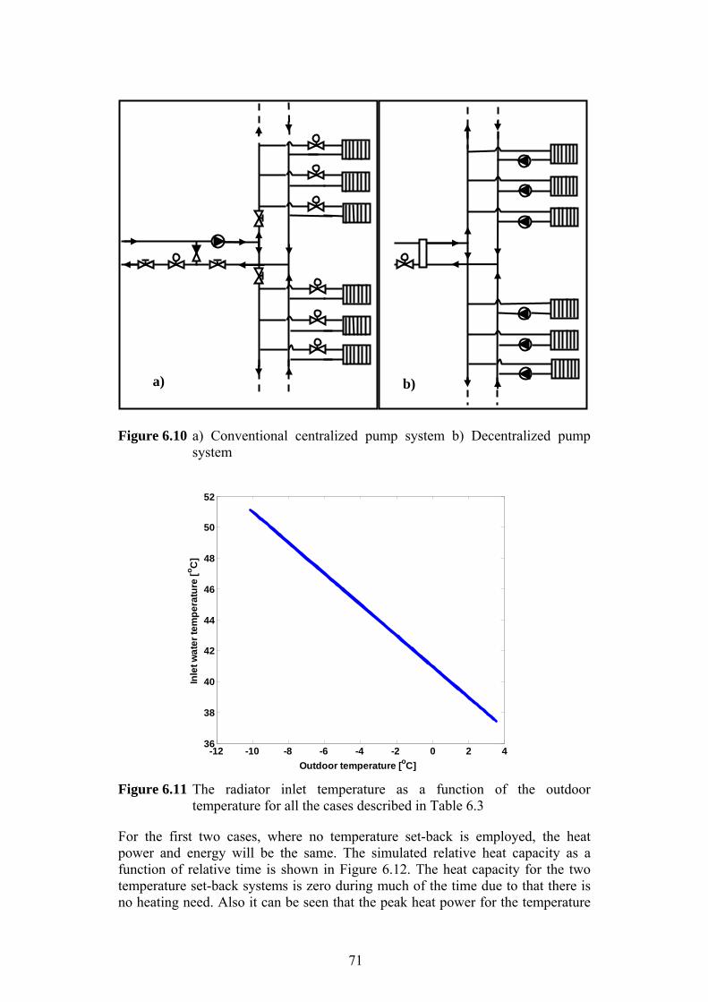
71

Figure 6.10 a) Conventional centralized pump system b) Decentralized pump system

Figure 6.11 The radiator inlet temperature as a function of the outdoor

temperature for all the cases described in Table 6.3

For the first two cases, where no temperature set-back is employed, the heat power and energy will be the same. The simulated relative heat capacity as a function of relative time is shown in Figure 6.12. The heat capacity for the two temperature set-back systems is zero during much of the time due to that there is no heating need. Also it can be seen that the peak heat power for the temperature

-12 -10 -8 -6 -4 -2 0 2 436

38

40

42

44

46

48

50

52

Outdoor temperature [oC]

Inle

t wa

ter

tem

pe

ratu

re [

oC

]

b) a)

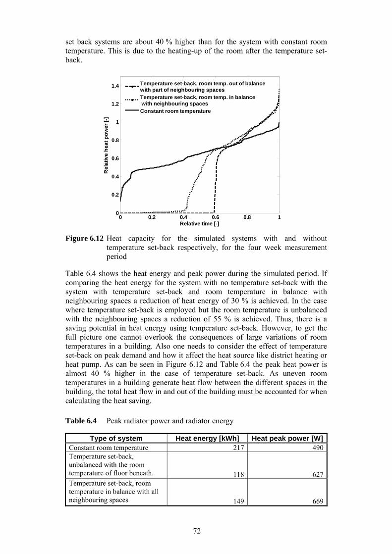
72

set back systems are about 40 % higher than for the system with constant room temperature. This is due to the heating-up of the room after the temperature set-back.

Figure 6.12 Heat capacity for the simulated systems with and without

temperature set-back respectively, for the four week measurement period

Table 6.4 shows the heat energy and peak power during the simulated period. If comparing the heat energy for the system with no temperature set-back with the system with temperature set-back and room temperature in balance with neighbouring spaces a reduction of heat energy of 30 % is achieved. In the case where temperature set-back is employed but the room temperature is unbalanced with the neighbouring spaces a reduction of 55 % is achieved. Thus, there is a saving potential in heat energy using temperature set-back. However, to get the full picture one cannot overlook the consequences of large variations of room temperatures in a building. Also one needs to consider the effect of temperature set-back on peak demand and how it affect the heat source like district heating or heat pump. As can be seen in Figure 6.12 and Table 6.4 the peak heat power is almost 40 % higher in the case of temperature set-back. As uneven room temperatures in a building generate heat flow between the different spaces in the building, the total heat flow in and out of the building must be accounted for when calculating the heat saving.

Table 6.4 Peak radiator power and radiator energy

Type of system Heat energy [kWh] Heat peak power [W] Constant room temperature 217 490 Temperature set-back, unbalanced with the room temperature of floor beneath. 118

627 Temperature set-back, room temperature in balance with all neighbouring spaces 149

669

0 0.2 0.4 0.6 0.8 10

0.2

0.4

0.6

0.8

1

1.2

1.4

Relative time [-]

Re

lati

ve

he

at

po

we

r [-

]

Temperature set-back, room temp. out of balancewith part of neighbouring spacesTemperature set-back, room temp. in balance with neighbouring spacesConstant room temperature

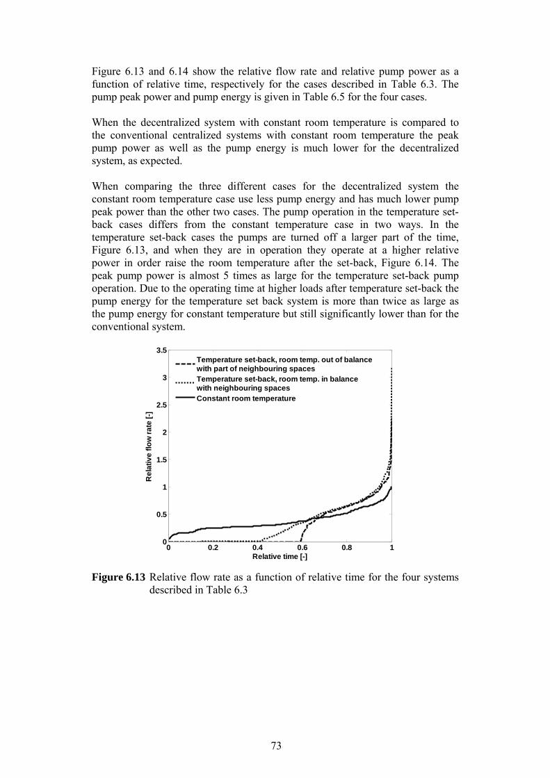
73

Figure 6.13 and 6.14 show the relative flow rate and relative pump power as a function of relative time, respectively for the cases described in Table 6.3. The pump peak power and pump energy is given in Table 6.5 for the four cases. When the decentralized system with constant room temperature is compared to the conventional centralized systems with constant room temperature the peak pump power as well as the pump energy is much lower for the decentralized system, as expected. When comparing the three different cases for the decentralized system the constant room temperature case use less pump energy and has much lower pump peak power than the other two cases. The pump operation in the temperature set-back cases differs from the constant temperature case in two ways. In the temperature set-back cases the pumps are turned off a larger part of the time, Figure 6.13, and when they are in operation they operate at a higher relative power in order raise the room temperature after the set-back, Figure 6.14. The peak pump power is almost 5 times as large for the temperature set-back pump operation. Due to the operating time at higher loads after temperature set-back the pump energy for the temperature set back system is more than twice as large as the pump energy for constant temperature but still significantly lower than for the conventional system.

Figure 6.13 Relative flow rate as a function of relative time for the four systems

described in Table 6.3

0 0.2 0.4 0.6 0.8 10

0.5

1

1.5

2

2.5

3

3.5

Relative time [-]

Re

lati

ve

flo

w r

ate

[-]

Temperature set-back, room temp. out of balancewith part of neighbouring spacesTemperature set-back, room temp. in balancewith neighbouring spacesConstant room temperature

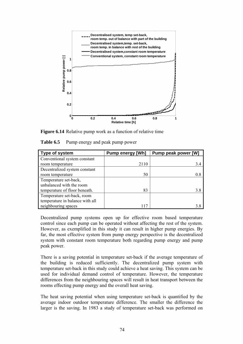
74

Figure 6.14 Relative pump work as a function of relative time

Table 6.5 Pump energy and peak pump power

Type of system Pump energy [Wh] Pump peak power [W] Conventional system constant room temperature 2110 3.4Decentralized system constant room temperature 50 0.8Temperature set-back, unbalanced with the room temperature of floor beneath. 83 3.8Temperature set-back, room temperature in balance with all neighbouring spaces 117 3.8 Decentralized pump systems open up for effective room based temperature control since each pump can be operated without affecting the rest of the system. However, as exemplified in this study it can result in higher pump energies. By far, the most effective system from pump energy perspective is the decentralized system with constant room temperature both regarding pump energy and pump peak power. There is a saving potential in temperature set-back if the average temperature of the building is reduced sufficiently. The decentralized pump system with temperature set-back in this study could achieve a heat saving. This system can be used for individual demand control of temperature. However, the temperature differences from the neighbouring spaces will result in heat transport between the rooms effecting pump energy and the overall heat saving. The heat saving potential when using temperature set-back is quantified by the average indoor outdoor temperature difference. The smaller the difference the larger is the saving. In 1983 a study of temperature set-back was performed on

0 0.2 0.4 0.6 0.8 10

0.2

0.4

0.6

0.8

1

Relative time [h]

Re

lati

ve

pu

mp

po

we

r [-

]

Decentralised system, temp set-back,room temp. out of balance with part of the buildingDecentralised system,temp. set-back,room temp. in balance with rest of the buildingDecentralised system,constant room temperatureConventional system, constant room temperature

75

multifamily houses in Sweden[43]. It showed an energy saving potential of only 4 %. In this study the indoor temperature decrease was only around 1 °C due to limitations in the radiator systems, occupancy behaviour and long thermal time constants of the buildings. The inlet temperature was decreased by 10 °C, which is the traditional temperature set-back control. In this simulation heat saving potential of 30 % during the measurement period was obtained due to larger indoor temperature decrease resulting in a smaller indoor outdoor temperature difference.

76

77

7 Case studies and laboratory tests A number of objects have been investigated through field and laboratory measurements. The objects range from buildings to components. In four case studies measurements in buildings has been conducted and in laboratory settings measurement of components (pumps, air coils, etc.) has been conducted. Case study I was the first measurement study made within this work. The pump electric power, water flow rate and inlet temperature of a radiator system in an office building was measured. The objective was to identify operational times, heating capacities and energy saving potential for pump operation. In Case study II a conventional radiator system where the capacity is controlled by mixing the supply and return water to the desired inlet temperature is rebuild to a decentralized pump system where every radiator is equipped with a small pump and where balancing and control valves are removed. In Case study III a run-around-loop heat exchanger, in a building used for service homes, has been examined and the optimal flow rate and pump energy saving potential has been calculated. In Case study IV the operation of air heater and air cooler in two air-handling units situated in a hospital building has been investigated. The time of operation, the capacities as well as the saving potential of using more efficient pump and fan operation been estimated. Laboratory measurement I had the main objective to investigate if pump manufacturers delivers what promised in their data sheets regarding capacity as well as efficiency. Efficiency and capacities of four pumps was measured. In Laboratory measurement II pump power of a fan-coil unit when the capacity was controlled by variable flow rate and constant inlet temperature was compared to capacity control by variable inlet temperature and constant flow rate. In Laboratory measurement III the heat transfer function of two cooling coils was measured when the cooling capacity was controlled by the flow rate. A model of the heat transfer function was validated.

7.1 Case study I: Conventional use of central VSD pumps

In an office building in Gothenburg the radiator system has been investigated. The aim of the study was to determine operational times and capacities and to estimate the saving potential of the pump power. It is a conventional radiator system where the capacity is controlled by mixing return and supply temperature to desired inlet temperature, see Figure 7.1. The electric power to the pump was measured. The radiator system is equipped with two parallel pumps with alternating operation every second week and a pump stop during summer time. The measurement was conducted over a heating season. Due to lack of equipment the electric power could only be measured for one of the pumps and therefore a measurement period

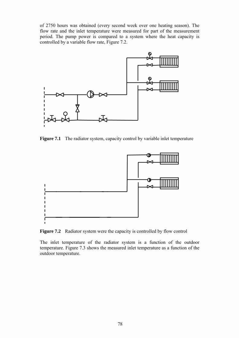
78

of 2750 hours was obtained (every second week over one heating season). The flow rate and the inlet temperature were measured for part of the measurement period. The pump power is compared to a system where the heat capacity is controlled by a variable flow rate, Figure 7.2.

Figure 7.1 The radiator system, capacity control by variable inlet temperature

Figure 7.2 Radiator system were the capacity is controlled by flow control The inlet temperature of the radiator system is a function of the outdoor temperature. Figure 7.3 shows the measured inlet temperature as a function of the outdoor temperature.

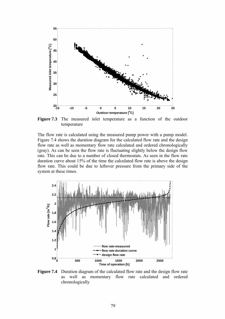
79

Figure 7.3 The measured inlet temperature as a function of the outdoor

temperature The flow rate is calculated using the measured pump power with a pump model. Figure 7.4 shows the duration diagram for the calculated flow rate and the design flow rate as well as momentary flow rate calculated and ordered chronologically (gray). As can be seen the flow rate is fluctuating slightly below the design flow rate. This can be due to a number of closed thermostats. As seen in the flow rate duration curve about 15% of the time the calculated flow rate is above the design flow rate. This could be due to leftover pressure from the primary side of the system at these times.

Figure 7.4 Duration diagram of the calculated flow rate and the design flow rate

as well as momentary flow rate calculated and ordered chronologically

-15 -10 -5 0 5 10 15 20 2520

25

30

35

40

45

50

55

Outdoor temperature [oC]

Mea

su

red

inle

t te

mp

era

ture

[oC

]

0 500 1000 1500 2000 25000.8

1

1.2

1.4

1.6

1.8

2

2.2

2.4

Time of operation [h]

Flo

w r

ate

[m3/h

]

flow rate-measuredflow rate-duration curvedesign flow rate

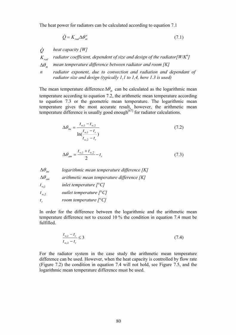
80

The heat power for radiators can be calculated according to equation 7.1

nmradKQ (7.1)

Q heat capacity [W]

radK radiator coefficient, dependent of size and design of the radiator[W/Kn]

m mean temperature difference between radiator and room [K]

n radiator exponent, due to convection and radiation and dependant of radiator size and design (typically 1,1 to 1,4, here 1.3 is used)

The mean temperature difference m can be calculated as the logarithmic mean

temperature according to equation 7.2, the arithmetic mean temperature according to equation 7.3 or the geometric mean temperature. The logarithmic mean temperature gives the most accurate result, however, the arithmetic mean temperature difference is usually good enough[67] for radiator calculations.

)ln(2,

1,

2,1,

rw

rw

wwlm

tt

tt

tt

(7.2)

rww

am ttt

2

2,1, (7.3)

lm logarithmic mean temperature difference [K]

am arithmetic mean temperature difference [K]

1,wt inlet temperature [°C]

2,wt outlet temperature [°C]

rt room temperature [°C] In order for the difference between the logarithmic and the arithmetic mean temperature difference not to exceed 10 % the condition in equation 7.4 must be fulfilled.

32

1

rw

rw

tt

tt

,

, (7.4)

For the radiator system in the case study the arithmetic mean temperature difference can be used. However, when the heat capacity is controlled by flow rate (Figure 7.2) the condition in equation 7.4 will not hold, see Figure 7.5, and the logarithmic mean temperature difference must be used.

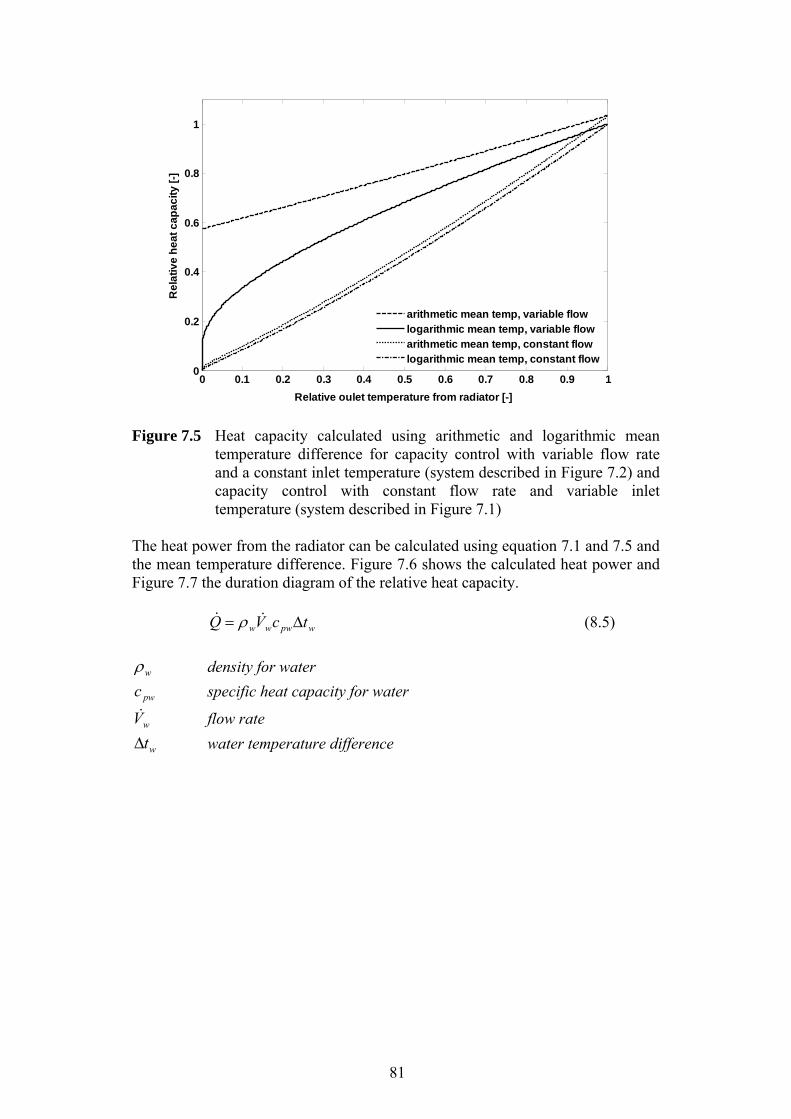
81

Figure 7.5 Heat capacity calculated using arithmetic and logarithmic mean

temperature difference for capacity control with variable flow rate and a constant inlet temperature (system described in Figure 7.2) and capacity control with constant flow rate and variable inlet temperature (system described in Figure 7.1)

The heat power from the radiator can be calculated using equation 7.1 and 7.5 and the mean temperature difference. Figure 7.6 shows the calculated heat power and Figure 7.7 the duration diagram of the relative heat capacity.

wpwww tcVQ (8.5)

w density for water

pwc specific heat capacity for water

wV flow rate

wt water temperature difference

0 0.1 0.2 0.3 0.4 0.5 0.6 0.7 0.8 0.9 10

0.2

0.4

0.6

0.8

1

Relative oulet temperature from radiator [-]

Re

lativ

e h

eat

cap

ac

ity [

-]

arithmetic mean temp, variable flowlogarithmic mean temp, variable flowarithmetic mean temp, constant flowlogarithmic mean temp, constant flow

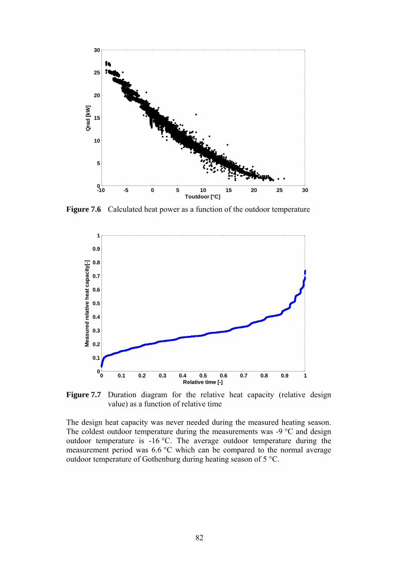
82

Figure 7.6 Calculated heat power as a function of the outdoor temperature

Figure 7.7 Duration diagram for the relative heat capacity (relative design

value) as a function of relative time The design heat capacity was never needed during the measured heating season. The coldest outdoor temperature during the measurements was -9 °C and design outdoor temperature is -16 °C. The average outdoor temperature during the measurement period was 6.6 °C which can be compared to the normal average outdoor temperature of Gothenburg during heating season of 5 °C.

-10 -5 0 5 10 15 20 25 300

5

10

15

20

25

30

Toutdoor [°C]

Qra

d [k

W]

0 0.1 0.2 0.3 0.4 0.5 0.6 0.7 0.8 0.9 10

0.1

0.2

0.3

0.4

0.5

0.6

0.7

0.8

0.9

1

Relative time [-]

Me

asu

red

re

lativ

e h

eat

cap

acit

y[-]

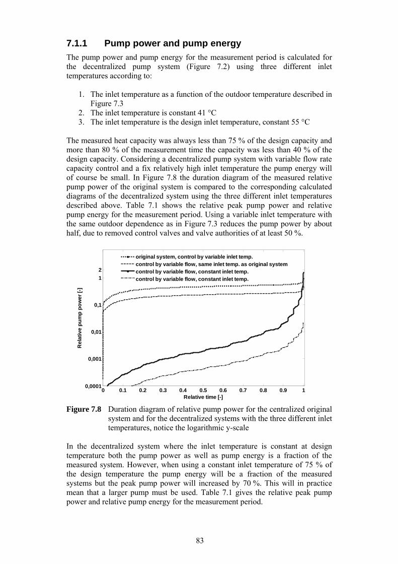
83

7.1.1 Pump power and pump energy

The pump power and pump energy for the measurement period is calculated for the decentralized pump system (Figure 7.2) using three different inlet temperatures according to:

1. The inlet temperature as a function of the outdoor temperature described in Figure 7.3

2. The inlet temperature is constant 41 °C 3. The inlet temperature is the design inlet temperature, constant 55 °C

The measured heat capacity was always less than 75 % of the design capacity and more than 80 % of the measurement time the capacity was less than 40 % of the design capacity. Considering a decentralized pump system with variable flow rate capacity control and a fix relatively high inlet temperature the pump energy will of course be small. In Figure 7.8 the duration diagram of the measured relative pump power of the original system is compared to the corresponding calculated diagrams of the decentralized system using the three different inlet temperatures described above. Table 7.1 shows the relative peak pump power and relative pump energy for the measurement period. Using a variable inlet temperature with the same outdoor dependence as in Figure 7.3 reduces the pump power by about half, due to removed control valves and valve authorities of at least 50 %.

Figure 7.8 Duration diagram of relative pump power for the centralized original

system and for the decentralized systems with the three different inlet temperatures, notice the logarithmic y-scale

In the decentralized system where the inlet temperature is constant at design temperature both the pump power as well as pump energy is a fraction of the measured system. However, when using a constant inlet temperature of 75 % of the design temperature the pump energy will be a fraction of the measured systems but the peak pump power will increased by 70 %. This will in practice mean that a larger pump must be used. Table 7.1 gives the relative peak pump power and relative pump energy for the measurement period.

0 0.1 0.2 0.3 0.4 0.5 0.6 0.7 0.8 0.9 10,0001

0,001

0,01

0,1

1

2

Relative time [-]

Re

lati

ve

pu

mp

po

we

r [-

]

original system, control by variable inlet temp. control by variable flow, same inlet temp. as original systemcontrol by variable flow, constant inlet temp.control by variable flow, constant inlet temp.

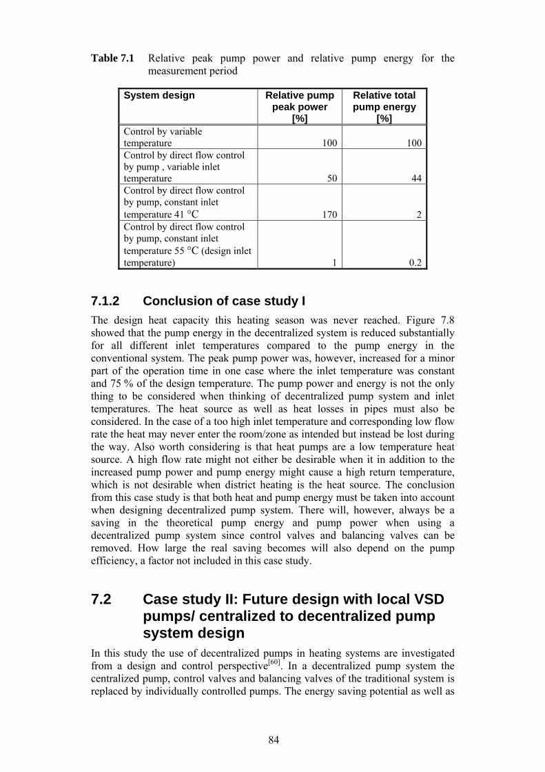
84

Table 7.1 Relative peak pump power and relative pump energy for the measurement period

System design Relative pump peak power

[%]

Relative total pump energy

[%] Control by variable temperature 100 100 Control by direct flow control by pump , variable inlet temperature 50 44 Control by direct flow control by pump, constant inlet temperature 41 °C 170 2 Control by direct flow control by pump, constant inlet temperature 55 °C (design inlet temperature) 1 0.2

7.1.2 Conclusion of case study I

The design heat capacity this heating season was never reached. Figure 7.8 showed that the pump energy in the decentralized system is reduced substantially for all different inlet temperatures compared to the pump energy in the conventional system. The peak pump power was, however, increased for a minor part of the operation time in one case where the inlet temperature was constant and 75 % of the design temperature. The pump power and energy is not the only thing to be considered when thinking of decentralized pump system and inlet temperatures. The heat source as well as heat losses in pipes must also be considered. In the case of a too high inlet temperature and corresponding low flow rate the heat may never enter the room/zone as intended but instead be lost during the way. Also worth considering is that heat pumps are a low temperature heat source. A high flow rate might not either be desirable when it in addition to the increased pump power and pump energy might cause a high return temperature, which is not desirable when district heating is the heat source. The conclusion from this case study is that both heat and pump energy must be taken into account when designing decentralized pump system. There will, however, always be a saving in the theoretical pump energy and pump power when using a decentralized pump system since control valves and balancing valves can be removed. How large the real saving becomes will also depend on the pump efficiency, a factor not included in this case study.

7.2 Case study II: Future design with local VSD pumps/ centralized to decentralized pump system design

In this study the use of decentralized pumps in heating systems are investigated from a design and control perspective[60]. In a decentralized pump system the centralized pump, control valves and balancing valves of the traditional system is replaced by individually controlled pumps. The energy saving potential as well as

85

pros and cons of decentralized systems are investigated. A radiator system of twenty radiators situated in a typical Swedish office building located in Gothenburg is used as a case study. In traditional radiator heating systems the heating capacity is controlled by a variable temperature. The temperature on the secondary side of the system is obtained by mixing supply and return water to desired inlet temperature. A more energy efficient way is direct flow control by variable speed pumps. The pump power is ideally proportional to the cube of the flow rate and accordingly the pump power will decrease substantially at reduced heating capacities. A further advantage is that no balancing of the system is required. A small radiator system is rebuilt from a temperature controlled system, described in Figure 7.9a, to a decentralized direct flow control system, Figure 7.9b. For every radiator in the system the thermostat is exchanged for a small variable speed pump. The radiator system consists of twenty radiators supplying heat to the top floor in an office building. This floor as well as its radiator system was added to the building in 1994. The office-floor consists of 11 rooms and is normally occupied during weekdays approximately between 7 am and 4 pm. Measurements of water flow rates, supply, inlet and return water temperatures, room temperatures, outdoor temperature, pump power are performed before and after rebuilding the system. The pre-rebuilding measurements were conducted for seven weeks under a period of late winter 2010. Measurements after rebuilding started during early winter 2010 and results from 6 weeks of measurements are presented. The result presented is for the radiator system situated at the top floor of the building.

Figure 7.9 a) The radiator system on the top floor before rebuilding (one central

pump) b) The radiator system after rebuilding (decentralized pumps) The primary side of the system supports the whole building (not only the top floor) and the supply temperature is already set. The supply temperature varies with the outdoor temperature according to Figure 7.10. This supply temperature curve is valid for the system both before and after rebuilding. The varying supply

b)

secondary side

primary side

a)

secondary side

primary side

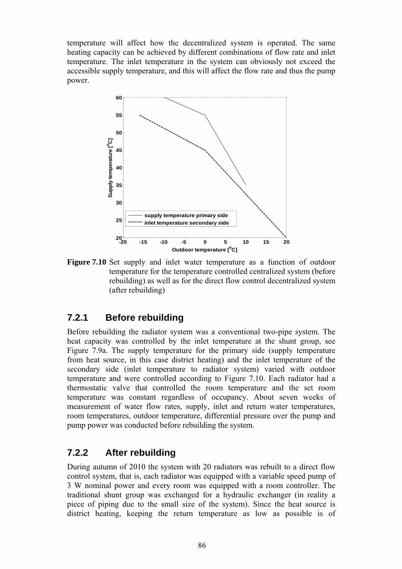
86

temperature will affect how the decentralized system is operated. The same heating capacity can be achieved by different combinations of flow rate and inlet temperature. The inlet temperature in the system can obviously not exceed the accessible supply temperature, and this will affect the flow rate and thus the pump power.

Figure 7.10 Set supply and inlet water temperature as a function of outdoor

temperature for the temperature controlled centralized system (before rebuilding) as well as for the direct flow control decentralized system (after rebuilding)

7.2.1 Before rebuilding

Before rebuilding the radiator system was a conventional two-pipe system. The heat capacity was controlled by the inlet temperature at the shunt group, see Figure 7.9a. The supply temperature for the primary side (supply temperature from heat source, in this case district heating) and the inlet temperature of the secondary side (inlet temperature to radiator system) varied with outdoor temperature and were controlled according to Figure 7.10. Each radiator had a thermostatic valve that controlled the room temperature and the set room temperature was constant regardless of occupancy. About seven weeks of measurement of water flow rates, supply, inlet and return water temperatures, room temperatures, outdoor temperature, differential pressure over the pump and pump power was conducted before rebuilding the system.

7.2.2 After rebuilding

During autumn of 2010 the system with 20 radiators was rebuilt to a direct flow control system, that is, each radiator was equipped with a variable speed pump of 3 W nominal power and every room was equipped with a room controller. The traditional shunt group was exchanged for a hydraulic exchanger (in reality a piece of piping due to the small size of the system). Since the heat source is district heating, keeping the return temperature as low as possible is of

-20 -15 -10 -5 0 5 10 15 2020

25

30

35

40

45

50

55

60

Outdoor temperature [oC]

Su

pp

ly tem

pera

ture

[oC

]

supply temperature primary side

inlet temperature secondary side

87

importance. For this reason a control valve was installed on the primary side to ensure low return temperature, see Figure 7.9b. The inlet temperature for the primary and secondary side varies with outside temperature and is controlled according to Figure 7.10. Table 7.2 shows the preset values for the room temperatures. Measurement started early winter 2010 and about 6 weeks of measurements are presented. Table 7.2 Set room temperatures after rebuilding the system Room temperature Offices and utility

rooms Server room

weekdays 7am-6pm 21.5 °C 18 °C night 6pm-7am and weekends 16 °C 18 °C

7.2.3 Pump energy results

Figure 7.11 shows the pump power as a function of relative heat capacity for the centralized (Figure 7.9a) and decentralized (Figure 7.9b) pump systems. Measurement sample time is 5 minutes and 1 minute for the centralized and the decentralized system respectively. Also the weekly average for the pump power is included. For the conventional centralized pump system (before rebuilding) the pump power is almost constant and unaffected by the heating capacity. One of the weekly average points for the decentralized system has a pump power higher than the rest of the weekly points; this is due to insufficient supply temperature. In systems with variable supply temperatures it can happen that for certain outdoor temperatures (usually mild temperatures) the supply temperature is not sufficiently high. Since the supply temperature is insufficient the pumps increases the flow rate in order to reach the set room temperature. In the measurement of the pump power in the decentralized system after rebuilding the power of the room controllers of 4 W is included in the measurement. For the decentralized pump system the dependency between heating capacity and pump power is not as visible as in the theoretical case. The main reason is that the supply and inlet water temperatures varies with the outdoor temperature (Figure 7.10) and this affects the flow rate and thus the pump power for a given heat capacity. However, the saving potential of at least 50 % at design capacity is clearly visible and also that the pump power decrease with decreased capacity. Additionally there are some odd data points that need to be addressed. There are a number of points at 4 W even for reasonably high relative heat capacities. As the power for the room controllers is 4 W it means that no pumps are switched on which means no flow rate. Since the flow rate is measured by a pulse meter which is counting pulses for a sample period it is possible that the pumps are switched off in the middle of a pulse counting period, and thus a flow rate is detected in spite of no pump power. The points with a relative heat capacity of zero or very close to zero but with maximum pump power have the same explanation. The pumps are switched on at the end of a pulse counting period and thus no flow rate is detected while pump power is measured.

88

Figure 7.11 Pump power as a function of relative flow rate for the centralized and

decentralized pump systems. Measurement sample time is 5 minutes and one minute for the centralized and the decentralized system respectively.

The average pump power for the measurement period was 49 W before rebuilding and 9.8 W after rebuilding which is a saving in pump power of 80 %. If only considering day time and accordingly not the night temperature set back, the average pump power after rebuilding is 13.9 W which is a saving in pump power of 71 %.

7.2.4 Heat energy results

In this case study temperature set-backs have been used for non-working hours (evenings and weekends) for the decentralized system after rebuilding. This can save heat energy. Also the controls of room temperatures are much better after rebuilding which gives additional savings. Figure 7.12 shows the weekly average of the measured heat power as a function of the outdoor temperature with fitted curves for the centralized system before rebuilding and the decentralized pumps system after rebuilding. The heat power demand in the decentralized pumps system is significantly lower than that of the centralized system. A part of the difference can be explained by the night- and weekend temperature set-back and a part of the difference can be explained by the leakage of heat from the floor beneath which has a constant room temperature. The two lines in Figure 7.12 are almost parallel which is expected since the only change to the system or building is the supplied heat power. The gradient for the fitted curves in Figure 7.12 can be used as an average UA-value (where U can be seen as the overall heat transfer coefficient and A the surface area on which U is based). Calculations of heat power for outdoor temperatures based on the UA-value and the indoor temperature, equation 7.6, is also included in Figure 7.12 (middle curve) and corresponds to a more realistic

0 0.2 0.4 0.6 0.8 10

10

20

30

40

50

60

70

Relative heating capacity [%]

Pu

mp

po

we

r [W

]

before rebuilding (temp. control by shunt group) after rebuilding (direct flow control by VSD pumps)

weekly avarage before rebuilding (temp. control by shunt group) weekly avarage efter rebuilding (direct flow control by VSD pumps)

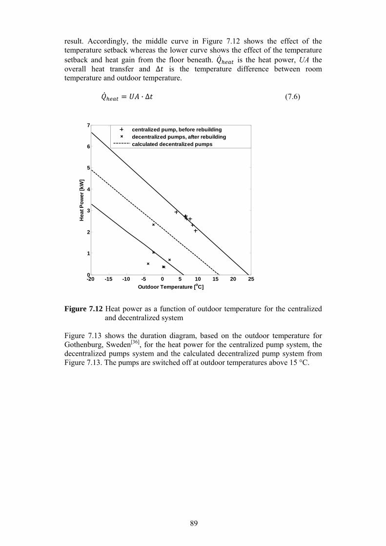
89

result. Accordingly, the middle curve in Figure 7.12 shows the effect of the temperature setback whereas the lower curve shows the effect of the temperature setback and heat gain from the floor beneath. is the heat power, UA the overall heat transfer and ∆ is the temperature difference between room temperature and outdoor temperature. · ∆ (7.6)

Figure 7.12 Heat power as a function of outdoor temperature for the centralized

and decentralized system Figure 7.13 shows the duration diagram, based on the outdoor temperature for Gothenburg, Sweden[36], for the heat power for the centralized pump system, the decentralized pumps system and the calculated decentralized pump system from Figure 7.13. The pumps are switched off at outdoor temperatures above 15 °C.

-20 -15 -10 -5 0 5 10 15 20 250

1

2

3

4

5

6

7

Outdoor Temperature [oC]

He

at P

ow

er [k

W]

centralized pump, before rebuildingdecentralized pumps, after rebuildingcalculated decentralized pumps

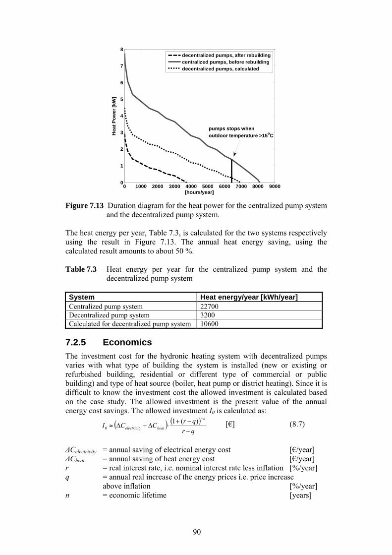
90

Figure 7.13 Duration diagram for the heat power for the centralized pump system

and the decentralized pump system. The heat energy per year, Table 7.3, is calculated for the two systems respectively using the result in Figure 7.13. The annual heat energy saving, using the calculated result amounts to about 50 %. Table 7.3 Heat energy per year for the centralized pump system and the

decentralized pump system System Heat energy/year [kWh/year] Centralized pump system 22700 Decentralized pump system 3200 Calculated for decentralized pump system 10600

7.2.5 Economics

The investment cost for the hydronic heating system with decentralized pumps varies with what type of building the system is installed (new or existing or refurbished building, residential or different type of commercial or public building) and type of heat source (boiler, heat pump or district heating). Since it is difficult to know the investment cost the allowed investment is calculated based on the case study. The allowed investment is the present value of the annual energy cost savings. The allowed investment I0 is calculated as:

qr

qrCCI

n

heatyelectricit

)(1

0 [€] (8.7)

ΔCelectricity = annual saving of electrical energy cost [€/year] ΔCheat = annual saving of heat energy cost [€/year] r = real interest rate, i.e. nominal interest rate less inflation [%/year] q = annual real increase of the energy prices i.e. price increase

above inflation [%/year] n = economic lifetime [years]

0 1000 2000 3000 4000 5000 6000 7000 8000 90000

1

2

3

4

5

6

7

8

[hours/year]

Heat P

ow

er

[kW

]

decentralized pumps, after rebuildingcentralized pumps, before rebuildingdecentralized pumps, calculated

pumps stops when

outdoor temperature >15oC

91

The present value factor is an approximation since the difference between the real interest rate and the annual real increase of the energy prices is used instead of the real interest rate. The real annual increase of the energy price is assumed to be the same for electrical and heat energy, respectively. If this is not the case the present value must be calculated for electricity and heat separately. For long-term investments proprietors typically have requirements on the nominal interest rate between 6 % and 10 %. If the inflation is assumed to be 2 % per year the requirement on the real interest rate is around 4 % to 8 %. The annual increase of the energy prices is an assumption for the unknown future and is mainly based on historical data. One reasonable assumption for the annual increase in energy prices is around 2 %. A different, maybe less reasonable, assumption is no real annual energy price increase at all. Consequently, the difference between the real interest rate and the real annual price increase of energy is between 2 % and 6 %. From a society point of view the real interest rate is often chosen around 4 %. The economic lifetime for hydronic heating systems is typically around 15 to 20 years. However, piping systems have an economic lifetime of 30 years. The thermostat parts of traditional thermostatic valves have a technical lifetime of about 10 years. Given the results from the case study the annual energy savings are: Electrical energy: 11 kWh per radiator Heat energy: 600 kWh per radiator If the electricity price is 0.13 €/kWh and the heat energy price is 0.09 €/kWh the total annual energy cost saving is 55 € per radiator and year. Given a real interest rate of 5 % (difference between the real interest rate and the real annual increase of the energy cost) and 15 years economic lifetime the allowed investment is 530 € per radiator.

7.2.6 Conclusion of case study II

In this study the use of decentralized pumps in heating systems are investigated from a design and control perspective. In a decentralized pump system the centralized pump, control and balancing valves of the traditional temperature controlled system is replaced by many individually controlled variable speed pumps. A small radiator system is rebuilt from a temperature controlled system to a decentralized direct flow control system. For every radiator in the system the thermostat is exchanged for a small variable speed pump. The results from the case study showed a saving potential in pump energy of about 70 % for the measurement period. For the system investigated in the case study the saving in “Watt” is not striking but considering the number of pumps installed in buildings and larger systems the saving potential is worth considering. Pumps in housing and commercial/public buildings in Sweden use about 1.5 % of the total electrical energy[57]. Results from the case study show a heat energy saving of 50 % during the measurement period. The energy saving comes from the use of temperature set-back during non-working hours. In order for temperature setback to be effective it

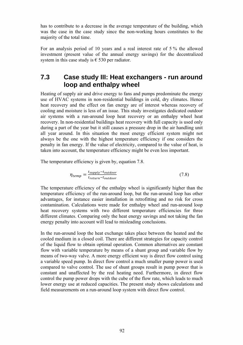
92

has to contribute to a decrease in the average temperature of the building, which was the case in the case study since the non-working hours constitutes to the majority of the total time. For an analysis period of 10 years and a real interest rate of 5 % the allowed investment (present value of the annual energy savings) for the decentralized system in this case study is € 530 per radiator.

7.3 Case study III: Heat exchangers - run around loop and enthalpy wheel

Heating of supply air and drive energy to fans and pumps predominate the energy use of HVAC systems in non-residential buildings in cold, dry climates. Hence heat recovery and the effect on fan energy are of interest whereas recovery of cooling and moisture is less of an issue. This study investigates dedicated outdoor air systems with a run-around loop heat recovery or an enthalpy wheel heat recovery. In non-residential buildings heat recovery with full capacity is used only during a part of the year but it still causes a pressure drop in the air handling unit all year around. In this situation the most energy efficient system might not always be the one with the highest temperature efficiency if one considers the penalty in fan energy. If the value of electricity, compared to the value of heat, is taken into account, the temperature efficiency might be even less important. The temperature efficiency is given by, equation 7.8.

(7.8)

The temperature efficiency of the enthalpy wheel is significantly higher than the temperature efficiency of the run-around loop, but the run-around loop has other advantages, for instance easier installation in retrofitting and no risk for cross contamination. Calculations were made for enthalpy wheel and run-around loop heat recovery systems with two different temperature efficiencies for three different climates. Comparing only the heat energy savings and not taking the fan energy penalty into account will lead to misleading conclusions. In the run-around loop the heat exchange takes place between the heated and the cooled medium in a closed coil. There are different strategies for capacity control of the liquid flow to obtain optimal operation. Common alternatives are constant flow with variable temperature by means of a shunt group and variable flow by means of two-way valve. A more energy efficient way is direct flow control using a variable speed pump. In direct flow control a much smaller pump power is used compared to valve control. The use of shunt groups result in pump power that is constant and unaffected by the real heating need. Furthermore, in direct flow control the pump power drops with the cube of the flow rate, which leads to much lower energy use at reduced capacities. The present study shows calculations and field measurements on a run-around loop system with direct flow control.

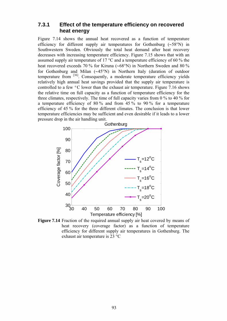
93

7.3.1 Effect of the temperature efficiency on recovered heat energy

Figure 7.14 shows the annual heat recovered as a function of temperature efficiency for different supply air temperatures for Gothenburg (58°N) in Southwestern Sweden. Obviously the total heat demand after heat recovery decreases with increasing temperature efficiency. Figure 7.15 shows that with an assumed supply air temperature of 17 °C and a temperature efficiency of 60 % the heat recovered exceeds 70 % for Kiruna (68°N) in Northern Sweden and 80 % for Gothenburg and Milan (45°N) in Northern Italy (duration of outdoor temperature from [36]. Consequently, a moderate temperature efficiency yields relatively high annual heat savings provided that the supply air temperature is controlled to a few °C lower than the exhaust air temperature. Figure 7.16 shows the relative time on full capacity as a function of temperature efficiency for the three climates, respectively. The time of full capacity varies from 0 % to 40 % for a temperature efficiency of 80 % and from 45 % to 90 % for a temperature efficiency of 45 % for the three different climates. The conclusion is that lower temperature efficiencies may be sufficient and even desirable if it leads to a lower pressure drop in the air handling unit.

Figure 7.14 Fraction of the required annual supply air heat covered by means of

heat recovery (coverage factor) as a function of temperature efficiency for different supply air temperatures in Gothenburg. The exhaust air temperature is 23 °C

30 40 50 60 70 80 90 10030

40

50

60

70

80

90

100

Temperature efficiency [%]

Co

vera

ge

fact

or

[%]

Gothenburg

Ts=12oC

Ts=14oC

Ts=16oC

Ts=18oC

Ts=20oC

94

Figure 7.15 Fraction of the required annual supply air heat covered by means of heat recovery (coverage factor) as a function of temperature efficiency with supply air temperature 17 °C in Milan, Gothenburg, and Kiruna. The exhaust air temperature is 23 °C

30 40 50 60 70 80 90 10030

40

50

60

70

80

90

100

Temperature efficiency [%]

Co

vera

ge

fact

or

[%]

Gothenburg

Kiruna

Milan

Relative time on full capacity=operating hours at:

Supply temperature = 17 °C Exhaust temperature = 23 °C

full capacity total hours of a year

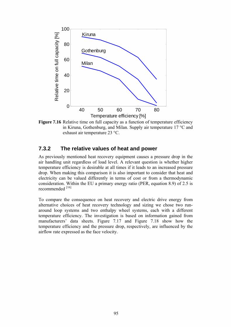
95

Figure 7.16 Relative time on full capacity as a function of temperature efficiency

in Kiruna, Gothenburg, and Milan. Supply air temperature 17 °C and exhaust air temperature 23 °C.

7.3.2 The relative values of heat and power

As previously mentioned heat recovery equipment causes a pressure drop in the air handling unit regardless of load level. A relevant question is whether higher temperature efficiency is desirable at all times if it leads to an increased pressure drop. When making this comparison it is also important to consider that heat and electricity can be valued differently in terms of cost or from a thermodynamic consideration. Within the EU a primary energy ratio (PER, equation 8.9) of 2.5 is recommended [16] To compare the consequence on heat recovery and electric drive energy from alternative choices of heat recovery technology and sizing we chose two run-around loop systems and two enthalpy wheel systems, each with a different temperature efficiency. The investigation is based on information gained from manufacturers’ data sheets. Figure 7.17 and Figure 7.18 show how the temperature efficiency and the pressure drop, respectively, are influenced by the airflow rate expressed as the face velocity.

40 50 60 70 800

20

40

60

80

100

Temperature efficiency [%]

Re

lativ

e ti

me

on

full

cap

aci

ty [%

]

Milan

Kiruna

Gothenburg

96

Figure 7.17 Temperature efficiency as a function of face velocity for enthalpy

wheels and run-around loops.

Figure 7.18 Pressure drop on the air side as a function of face velocity for

enthalpy wheels and run-around loops. For face velocities below and around 2 m/s the air flow is mainly laminar and the pressure drop is comparable for the two types of heat recovery systems as shown in Figure 7.18. Still the temperature efficiency is considerably better for the enthalpy wheel as shown in Figure 7.17. The trend in modern design is to upsize the air-handling units to reduce the face velocity. Typical face velocities in Northern Europe are 1.5 to 2.0 m/s. Provided reasonable pressure drops in the distribution system and a high total fan efficiency this results in a Specific Fan Power of 1.5 to 2.0 kW/(m3/s) at design air flow, including an air-to-air heat recovery unit.

0 1 2 3 4 540

50

60

70

80

90

100

Te

mp

era

ture

effi

cie

ncy

[%]

Face velocity [m/s]

Run-around loops

Enthalpy wheels

0 1 2 3 4 50

200

400

600

800

1000

1200

Face velocity [m/s]

Pre

ssu

re d

rop

[Pa

]

Run-around loops

Enthalpy wheels

97

When considering a heat recovery system the electric energy consumed for driving the fan to overcome the heat recovery pressure drop must be taken into account. As previously mentioned the value of electrical energy is usually higher in terms of cost (Energy cost ratio, ECR) and also considered to be higher in terms of thermodynamic potential (Primary energy ratio, PER) than heat, equation 7.9.

, (7.9)

In order not to complicate the message by making a priori assumption on PER or ECR we present results on recovered heat and additional fan and pump energy in terms of a heat recovery coefficient of performance, equation 7.10.

, , (7.10)

Figure 7.19 and Figure 7.20 show the coefficient of performance for the enthalpy wheel and run-around loop respectively. To select the best alternative in consideration of PER or ECR the COPHRV values can be divided by the respective ratio. This is also included with PER=2.5.

Figure 7.19 The coefficient of performance of enthalpy wheel heat recovery,

COPHRV, as a function of air flow rate for Gothenburg, supply air temperature 16 °C and exhaust air temperature 23 °C

0.5 1 1.5 2 2.5 30

50

100

150

Air flow [m3/s]

CO

PH

RV [-

]

Enthalpy wheel

higher efficiencylower efficiency

PER=2.5

PER=1

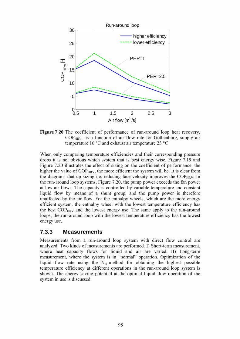
98

Figure 7.20 The coefficient of performance of run-around loop heat recovery,

COPHRV, as a function of air flow rate for Gothenburg, supply air temperature 16 °C and exhaust air temperature 23 °C

When only comparing temperature efficiencies and their corresponding pressure drops it is not obvious which system that is best energy wise. Figure 7.19 and Figure 7.20 illustrates the effect of sizing on the coefficient of performance, the higher the value of COPHRV, the more efficient the system will be. It is clear from the diagrams that up sizing i.e. reducing face velocity improves the COPHRV. In the run-around loop systems, Figure 7.20, the pump power exceeds the fan power at low air flows. The capacity is controlled by variable temperature and constant liquid flow by means of a shunt group, and the pump power is therefore unaffected by the air flow. For the enthalpy wheels, which are the more energy efficient system, the enthalpy wheel with the lowest temperature efficiency has the best COPHRV and the lowest energy use. The same apply to the run-around loops; the run-around loop with the lowest temperature efficiency has the lowest energy use.

7.3.3 Measurements

Measurements from a run-around loop system with direct flow control are analyzed. Two kinds of measurements are performed. I) Short-term measurement, where heat capacity flows for liquid and air are varied. II) Long-term measurement, where the system is in “normal” operation. Optimization of the liquid flow rate using the Ntu-method for obtaining the highest possible temperature efficiency at different operations in the run-around loop system is shown. The energy saving potential at the optimal liquid flow operation of the system in use is discussed.

0.5 1 1.5 2 2.5 30

5

10

15

20

25

30

Air flow [m3/s]

CO

PH

RV [-

]

Run-around loop

higher efficiencylower efficiency

PER=2.5

PER=1

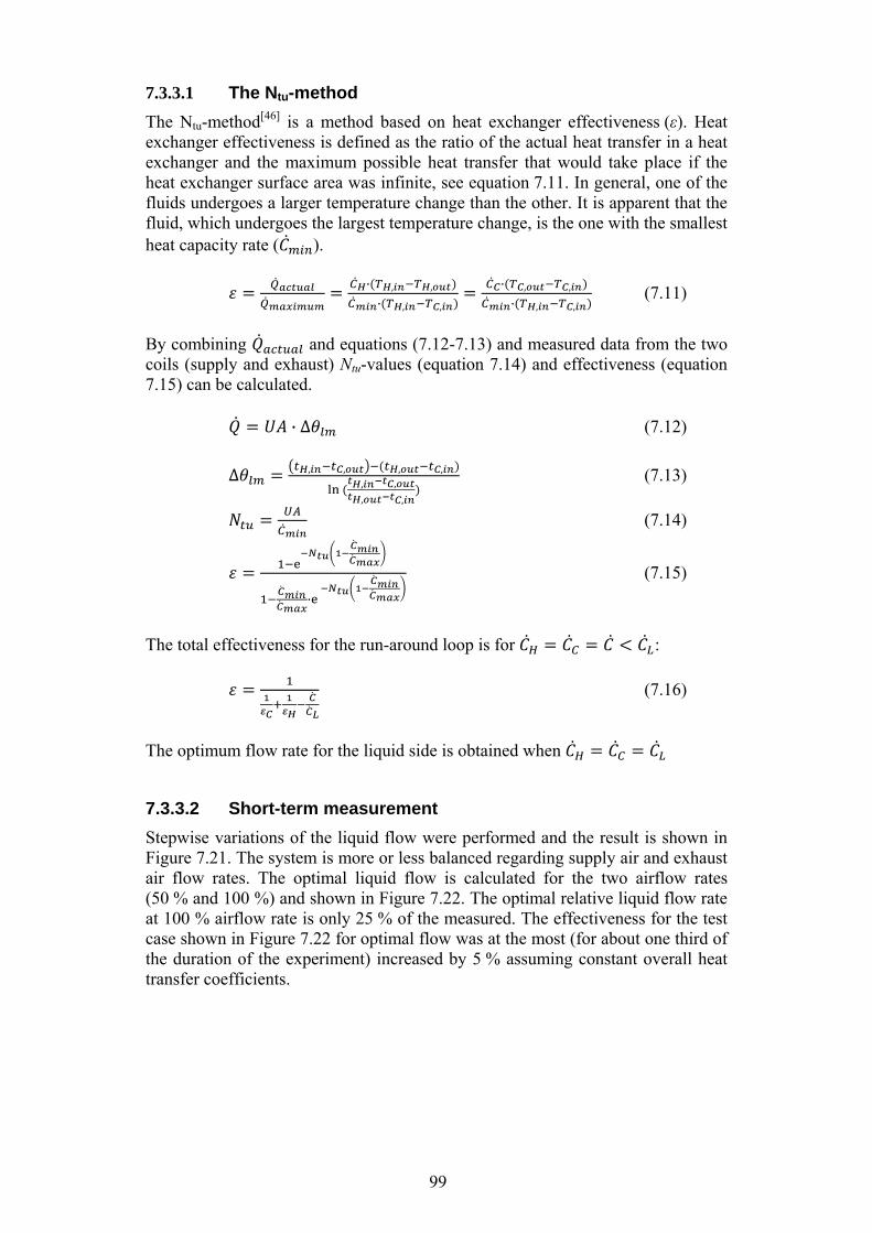
99

7.3.3.1 The Ntu-method

The Ntu-method[46] is a method based on heat exchanger effectiveness (ε). Heat exchanger effectiveness is defined as the ratio of the actual heat transfer in a heat exchanger and the maximum possible heat transfer that would take place if the heat exchanger surface area was infinite, see equation 7.11. In general, one of the fluids undergoes a larger temperature change than the other. It is apparent that the fluid, which undergoes the largest temperature change, is the one with the smallest heat capacity rate ( ).

· , ,

· , ,

· , ,

· , , (7.11)

By combining and equations (7.12-7.13) and measured data from the two coils (supply and exhaust) Ntu-values (equation 7.14) and effectiveness (equation 7.15) can be calculated. · ∆ (7.12)

∆ , , , ,

, ,

, ,

(7.13)

(7.14)

·

(7.15)

The total effectiveness for the run-around loop is for :

(7.16)

The optimum flow rate for the liquid side is obtained when

7.3.3.2 Short-term measurement

Stepwise variations of the liquid flow were performed and the result is shown in Figure 7.21. The system is more or less balanced regarding supply air and exhaust air flow rates. The optimal liquid flow is calculated for the two airflow rates (50 % and 100 %) and shown in Figure 7.22. The optimal relative liquid flow rate at 100 % airflow rate is only 25 % of the measured. The effectiveness for the test case shown in Figure 7.22 for optimal flow was at the most (for about one third of the duration of the experiment) increased by 5 % assuming constant overall heat transfer coefficients.

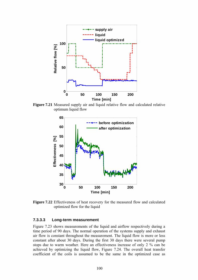
100

Figure 7.21 Measured supply air and liquid relative flow and calculated relative

optimum liquid flow

Figure 7.22 Effectiveness of heat recovery for the measured flow and calculated

optimized flow for the liquid

7.3.3.3 Long-term measurement

Figure 7.23 shows measurements of the liquid and airflow respectively during a time period of 90 days. The normal operation of the systems supply and exhaust air flow is constant throughout the measurement. The liquid flow is more or less constant after about 30 days. During the first 30 days there were several pump stops due to warm weather. Here an effectiveness increase of only 2 % can be achieved by optimizing the liquid flow, Figure 7.24. The overall heat transfer coefficient of the coils is assumed to be the same in the optimized case as

0 50 100 150 2000

50

100

Time [min]

Rel

ativ

e fl

ow

[%

]

supply air

liquidliquid optimized

0 50 100 150 20030

35

40

45

50

55

60

65

Time [min]

Eff

ecti

ven

ess

[%

]

before optimization

after optimization

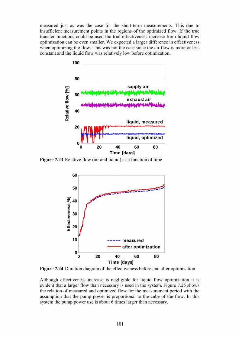
101

measured just as was the case for the short-term measurements. This due to insufficient measurement points in the regions of the optimized flow. If the true transfer functions could be used the true effectiveness increase from liquid flow optimization can be even smaller. We expected a larger difference in effectiveness when optimizing the flow. This was not the case since the air flow is more or less constant and the liquid flow was relatively low before optimization.

Figure 7.23 Relative flow (air and liquid) as a function of time

Figure 7.24 Duration diagram of the effectiveness before and after optimization Although effectiveness increase is negligible for liquid flow optimization it is evident that a larger flow than necessary is used in the system. Figure 7.25 shows the relation of measured and optimized flow for the measurement period with the assumption that the pump power is proportional to the cube of the flow. In this system the pump power use is about 6 times larger than necessary.

0 20 40 60 800

20

40

60

80

100

Time [days]

Rel

ativ

e fl

ow

[%

]

liquid, measured

supply air

liquid, optimized

exhaust air

0 20 40 60 800

10

20

30

40

50

60

Time [days]

Eff

ecti

ven

ess[

%]

measured

after optimization

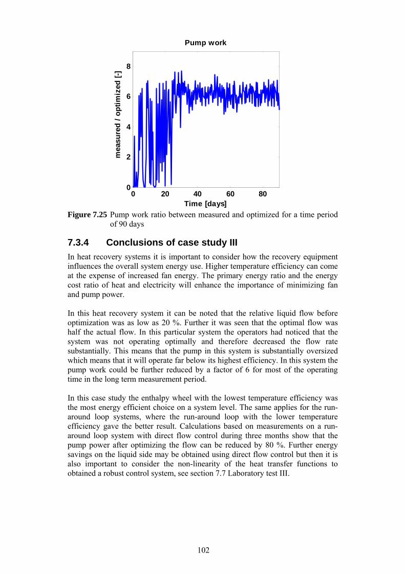
102

Figure 7.25 Pump work ratio between measured and optimized for a time period

of 90 days

7.3.4 Conclusions of case study III

In heat recovery systems it is important to consider how the recovery equipment influences the overall system energy use. Higher temperature efficiency can come at the expense of increased fan energy. The primary energy ratio and the energy cost ratio of heat and electricity will enhance the importance of minimizing fan and pump power. In this heat recovery system it can be noted that the relative liquid flow before optimization was as low as 20 %. Further it was seen that the optimal flow was half the actual flow. In this particular system the operators had noticed that the system was not operating optimally and therefore decreased the flow rate substantially. This means that the pump in this system is substantially oversized which means that it will operate far below its highest efficiency. In this system the pump work could be further reduced by a factor of 6 for most of the operating time in the long term measurement period. In this case study the enthalpy wheel with the lowest temperature efficiency was the most energy efficient choice on a system level. The same applies for the run-around loop systems, where the run-around loop with the lower temperature efficiency gave the better result. Calculations based on measurements on a run-around loop system with direct flow control during three months show that the pump power after optimizing the flow can be reduced by 80 %. Further energy savings on the liquid side may be obtained using direct flow control but then it is also important to consider the non-linearity of the heat transfer functions to obtained a robust control system, see section 7.7 Laboratory test III.

0 20 40 60 800

2

4

6

8

Time [days]

mea

sure

d /

op

tim

ized

[-]

Pump work

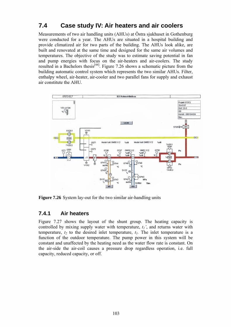
103

7.4 Case study IV: Air heaters and air coolers Measurements of two air handling units (AHUs) at Östra sjukhuset in Gothenburg were conducted for a year. The AHUs are situated in a hospital building and provide climatized air for two parts of the building. The AHUs look alike, are built and renovated at the same time and designed for the same air volumes and temperatures. The objective of the study was to estimate saving potential in fan and pump energies with focus on the air-heaters and air-coolers. The study resulted in a Bachelors thesis[44]. Figure 7.26 shows a schematic picture from the building automatic control system which represents the two similar AHUs. Filter, enthalpy wheel, air-heater, air-cooler and two parallel fans for supply and exhaust air constitute the AHU.

Figure 7.26 System lay-out for the two similar air-handling units

7.4.1 Air heaters

Figure 7.27 shows the layout of the shunt group. The heating capacity is controlled by mixing supply water with temperature, t1’, and returns water with temperature, t2 to the desired inlet temperature, t1. The inlet temperature is a function of the outdoor temperature. The pump power in this system will be constant and unaffected by the heating need as the water flow rate is constant. On the air-side the air-coil causes a pressure drop regardless operation, i.e. full capacity, reduced capacity, or off.

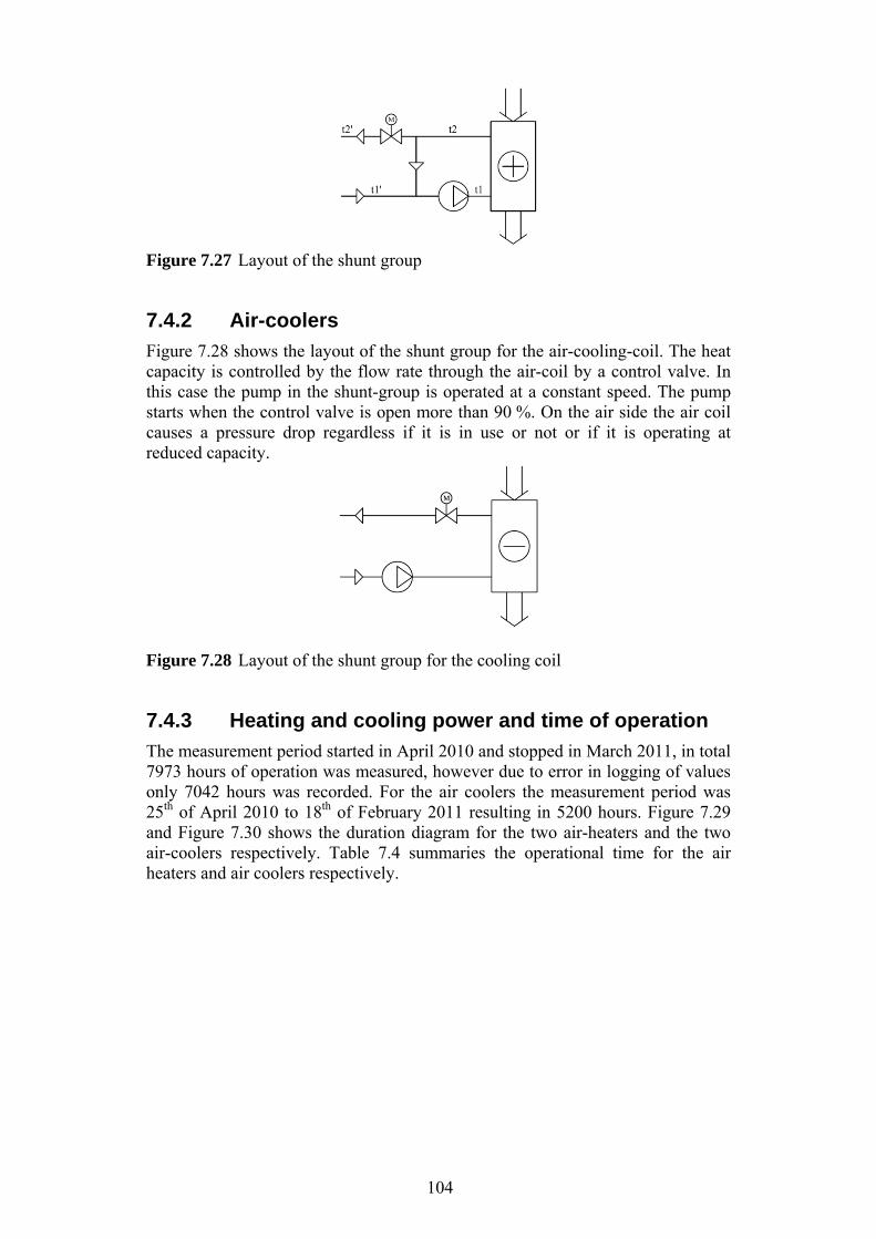
104

Figure 7.27 Layout of the shunt group

7.4.2 Air-coolers

Figure 7.28 shows the layout of the shunt group for the air-cooling-coil. The heat capacity is controlled by the flow rate through the air-coil by a control valve. In this case the pump in the shunt-group is operated at a constant speed. The pump starts when the control valve is open more than 90 %. On the air side the air coil causes a pressure drop regardless if it is in use or not or if it is operating at reduced capacity.

Figure 7.28 Layout of the shunt group for the cooling coil

7.4.3 Heating and cooling power and time of operation

The measurement period started in April 2010 and stopped in March 2011, in total 7973 hours of operation was measured, however due to error in logging of values only 7042 hours was recorded. For the air coolers the measurement period was 25th of April 2010 to 18th of February 2011 resulting in 5200 hours. Figure 7.29 and Figure 7.30 shows the duration diagram for the two air-heaters and the two air-coolers respectively. Table 7.4 summaries the operational time for the air heaters and air coolers respectively.

105

Figure 7.29 Duration diagram for the two air-heaters in AHU 1 and AHU 2

Figure 7.30 Duration diagram for the two air-coolers in AHU 1 and AHU 2 Table 7.4 Operational time of air heater and air cooler in the two air-handling-

units

AHU 1 AHU 2

Time of operation for air-heaters [h] 2550 2700

Time of operation for air-coolers [h] 1450 550

The air-cooler in AHU 2 is in operation only 550 hours during the measurement period and the maximum cooling power is about 60 % of design value. The average capacity during operation is 8 % of design value. For the air heater in

0 0.2 0.4 0.6 0.8 10

0.1

0.2

0.3

0.4

0.5

0.6

0.7

0.8

0.9

1

Relative time [%]

Re

lati

ve

he

at

ca

pa

city

[k

W]

air-heater AHU 1

air-heater AHU 2

0 0.2 0.4 0.6 0.8 10

0.1

0.2

0.3

0.4

0.5

0.6

0.7

0.8

0.9

1

Relative time [-]

Re

lati

ve

co

olin

g c

ap

ac

ity

[-]

air-cooler AHU1

air-cooler AHU2

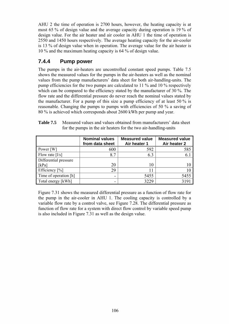
106

AHU 2 the time of operation is 2700 hours, however, the heating capacity is at most 65 % of design value and the average capacity during operation is 19 % of design value. For the air heater and air cooler in AHU 1 the time of operation is 2550 and 1450 hours respectively. The average heating capacity for the air-cooler is 13 % of design value when in operation. The average value for the air heater is 10 % and the maximum heating capacity is 64 % of design value.

7.4.4 Pump power

The pumps in the air-heaters are uncontrolled constant speed pumps. Table 7.5 shows the measured values for the pumps in the air-heaters as well as the nominal values from the pump manufacturers’ data sheet for both air-handling-units. The pump efficiencies for the two pumps are calculated to 11 % and 10 % respectively which can be compared to the efficiency stated by the manufacturer of 30 %. The flow rate and the differential pressure do never reach the nominal values stated by the manufacturer. For a pump of this size a pump efficiency of at least 50 % is reasonable. Changing the pumps to pumps with efficiencies of 50 % a saving of 80 % is achieved which corresponds about 2600 kWh per pump and year. Table 7.5 Measured values and values obtained from manufacturers’ data sheet

for the pumps in the air heaters for the two air-handling-units

Nominal values from data sheet

Measured valueAir heater 1

Measured value Air heater 2

Power [W] 600 592 585Flow rate [l/s] 8.7 6.3 6.1Differential pressure [kPa] 20 10 10Efficiency [%] 29 11 10Time of operation [h] - 5455 5455Total energy [kWh] - 3229 3191 Figure 7.31 shows the measured differential pressure as a function of flow rate for the pump in the air-cooler in AHU 1. The cooling capacity is controlled by a variable flow rate by a control valve, see Figure 7.28. The differential pressure as function of flow rate for a system with direct flow control by variable speed pump is also included in Figure 7.31 as well as the design value.

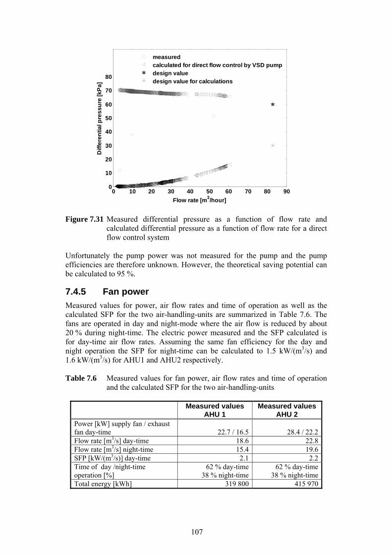
107

Figure 7.31 Measured differential pressure as a function of flow rate and calculated differential pressure as a function of flow rate for a direct flow control system

Unfortunately the pump power was not measured for the pump and the pump efficiencies are therefore unknown. However, the theoretical saving potential can be calculated to 95 %.

7.4.5 Fan power

Measured values for power, air flow rates and time of operation as well as the calculated SFP for the two air-handling-units are summarized in Table 7.6. The fans are operated in day and night-mode where the air flow is reduced by about 20 % during night-time. The electric power measured and the SFP calculated is for day-time air flow rates. Assuming the same fan efficiency for the day and night operation the SFP for night-time can be calculated to 1.5 kW/(m3/s) and 1.6 kW/(m3/s) for AHU1 and AHU2 respectively. Table 7.6 Measured values for fan power, air flow rates and time of operation

and the calculated SFP for the two air-handling-units

Measured valuesAHU 1

Measured values AHU 2

Power [kW] supply fan / exhaust fan day-time

22.7 / 16.5

28.4 / 22.2

Flow rate [m3/s] day-time 18.6 22.8 Flow rate [m3/s] night-time 15.4 19.6 SFP [kW/(m3/s)] day-time 2.1 2.2 Time of day /night-time operation [%]

62 % day-time 38 % night-time

62 % day-time 38 % night-time

Total energy [kWh] 319 800 415 970

0 10 20 30 40 50 60 70 80 900

10

20

30

40

50

60

70

80

Flow rate [m3/hour]

Dif

fere

ntia

l pre

ssu

re [

kPa]

measuredcalculated for direct flow control by VSD pumpdesign valuedesign value for calculations

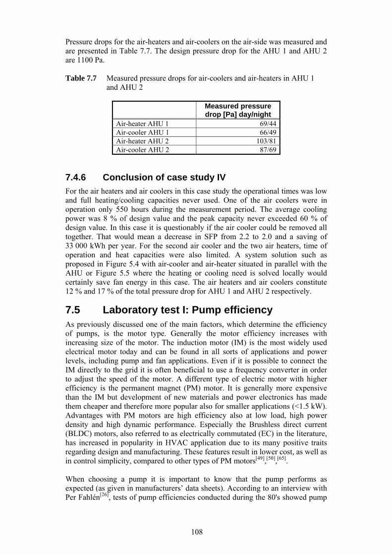
108

Pressure drops for the air-heaters and air-coolers on the air-side was measured and are presented in Table 7.7. The design pressure drop for the AHU 1 and AHU 2 are 1100 Pa. Table 7.7 Measured pressure drops for air-coolers and air-heaters in AHU 1

and AHU 2

Measured pressure drop [Pa] day/night

Air-heater AHU 1 69/44Air-cooler AHU 1 66/49Air-heater AHU 2 103/81Air-cooler AHU 2 87/69

7.4.6 Conclusion of case study IV

For the air heaters and air coolers in this case study the operational times was low and full heating/cooling capacities never used. One of the air coolers were in operation only 550 hours during the measurement period. The average cooling power was 8 % of design value and the peak capacity never exceeded 60 % of design value. In this case it is questionably if the air cooler could be removed all together. That would mean a decrease in SFP from 2.2 to 2.0 and a saving of 33 000 kWh per year. For the second air cooler and the two air heaters, time of operation and heat capacities were also limited. A system solution such as proposed in Figure 5.4 with air-cooler and air-heater situated in parallel with the AHU or Figure 5.5 where the heating or cooling need is solved locally would certainly save fan energy in this case. The air heaters and air coolers constitute 12 % and 17 % of the total pressure drop for AHU 1 and AHU 2 respectively.

7.5 Laboratory test I: Pump efficiency As previously discussed one of the main factors, which determine the efficiency of pumps, is the motor type. Generally the motor efficiency increases with increasing size of the motor. The induction motor (IM) is the most widely used electrical motor today and can be found in all sorts of applications and power levels, including pump and fan applications. Even if it is possible to connect the IM directly to the grid it is often beneficial to use a frequency converter in order to adjust the speed of the motor. A different type of electric motor with higher efficiency is the permanent magnet (PM) motor. It is generally more expensive than the IM but development of new materials and power electronics has made them cheaper and therefore more popular also for smaller applications (<1.5 kW). Advantages with PM motors are high efficiency also at low load, high power density and high dynamic performance. Especially the Brushless direct current (BLDC) motors, also referred to as electrically commutated (EC) in the literature, has increased in popularity in HVAC application due to its many positive traits regarding design and manufacturing. These features result in lower cost, as well as in control simplicity, compared to other types of PM motors[49],[50],[65]. When choosing a pump it is important to know that the pump performs as expected (as given in manufacturers’ data sheets). According to an interview with Per Fahlén[26], tests of pump efficiencies conducted during the 80's showed pump

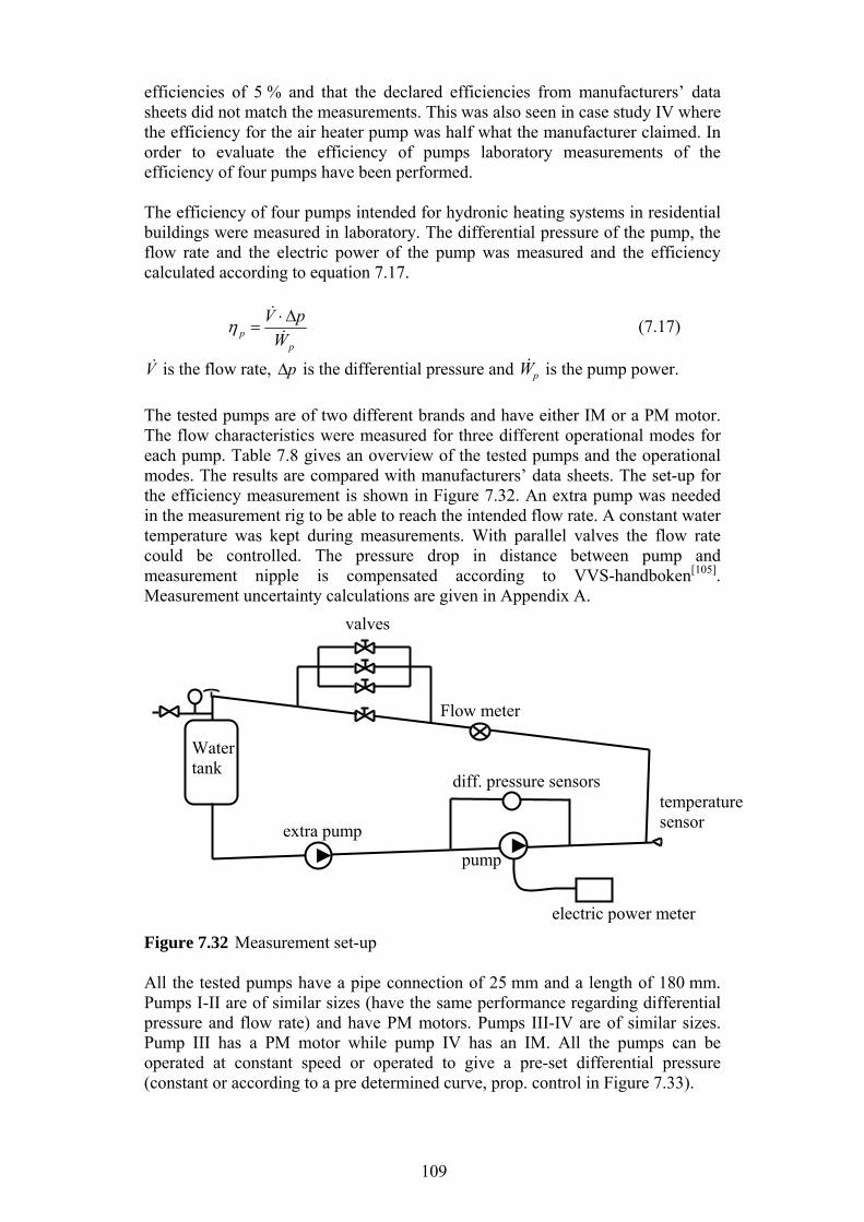
109

efficiencies of 5 % and that the declared efficiencies from manufacturers’ data sheets did not match the measurements. This was also seen in case study IV where the efficiency for the air heater pump was half what the manufacturer claimed. In order to evaluate the efficiency of pumps laboratory measurements of the efficiency of four pumps have been performed. The efficiency of four pumps intended for hydronic heating systems in residential buildings were measured in laboratory. The differential pressure of the pump, the flow rate and the electric power of the pump was measured and the efficiency calculated according to equation 7.17.

pp W

pV

(7.17)

V is the flow rate, p is the differential pressure and pW is the pump power.

The tested pumps are of two different brands and have either IM or a PM motor. The flow characteristics were measured for three different operational modes for each pump. Table 7.8 gives an overview of the tested pumps and the operational modes. The results are compared with manufacturers’ data sheets. The set-up for the efficiency measurement is shown in Figure 7.32. An extra pump was needed in the measurement rig to be able to reach the intended flow rate. A constant water temperature was kept during measurements. With parallel valves the flow rate could be controlled. The pressure drop in distance between pump and measurement nipple is compensated according to VVS-handboken[105]. Measurement uncertainty calculations are given in Appendix A.

Figure 7.32 Measurement set-up All the tested pumps have a pipe connection of 25 mm and a length of 180 mm. Pumps I-II are of similar sizes (have the same performance regarding differential pressure and flow rate) and have PM motors. Pumps III-IV are of similar sizes. Pump III has a PM motor while pump IV has an IM. All the pumps can be operated at constant speed or operated to give a pre-set differential pressure (constant or according to a pre determined curve, prop. control in Figure 7.33).

electric power meter

extra pump

diff. pressure sensors

Flow meter

pump

Water tank

valves

temperature sensor

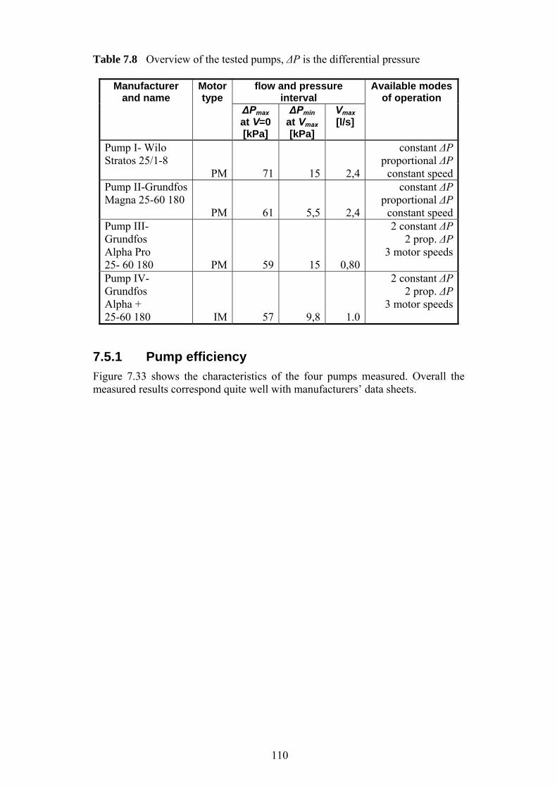
110

Table 7.8 Overview of the tested pumps, ΔP is the differential pressure

Manufacturer and name

Motor type

flow and pressure interval

Available modes of operation

ΔPmax at V=0 [kPa]

ΔPmin at Vmax

[kPa]

Vmax

[l/s]

Pump I- Wilo Stratos 25/1-8

PM 71 15 2,4

constant ΔP proportional ΔP

constant speed Pump II-Grundfos Magna 25-60 180

PM 61 5,5 2,4

constant ΔP proportional ΔP

constant speed Pump III-Grundfos Alpha Pro 25- 60 180

PM 59 15 0,80

2 constant ΔP 2 prop. ΔP

3 motor speeds

Pump IV-Grundfos Alpha + 25-60 180

IM 57 9,8 1.0

2 constant ΔP 2 prop. ΔP

3 motor speeds

7.5.1 Pump efficiency

Figure 7.33 shows the characteristics of the four pumps measured. Overall the measured results correspond quite well with manufacturers’ data sheets.

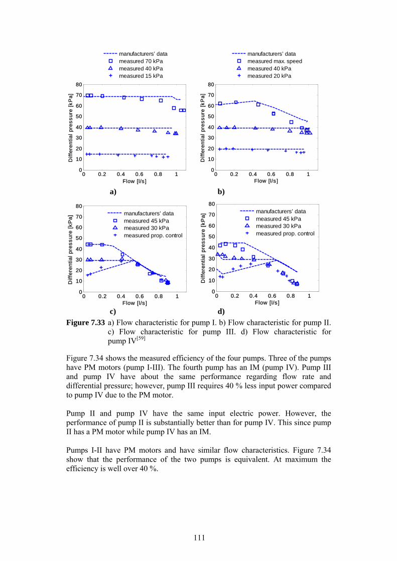
111

a) b)

c) d)

Figure 7.33 a) Flow characteristic for pump I. b) Flow characteristic for pump II. c) Flow characteristic for pump III. d) Flow characteristic for pump IV[59]

Figure 7.34 shows the measured efficiency of the four pumps. Three of the pumps have PM motors (pump I-III). The fourth pump has an IM (pump IV). Pump III and pump IV have about the same performance regarding flow rate and differential pressure; however, pump III requires 40 % less input power compared to pump IV due to the PM motor. Pump II and pump IV have the same input electric power. However, the performance of pump II is substantially better than for pump IV. This since pump II has a PM motor while pump IV has an IM. Pumps I-II have PM motors and have similar flow characteristics. Figure 7.34 show that the performance of the two pumps is equivalent. At maximum the efficiency is well over 40 %.

0 0.2 0.4 0.6 0.8 10

10

20

30

40

50

60

70

80

Flow [l/s ]

Dif

fere

nti

al

pre

ss

ure

[k

Pa

]

manufacturers’ datameasured 70 kPameasured 40 kPameasured 15 kPa

0 0.2 0.4 0.6 0.8 10

10

20

30

40

50

60

70

80

Flow [l/s ]

Dif

fere

nti

al

pre

ss

ure

[k

Pa

]

manufacturers’ datameasured max. speedmeasured 40 kPameasured 20 kPa

0 0.2 0.4 0.6 0.8 10

10

20

30

40

50

60

70

80

Flow [l/s ]

Dif

fere

nti

al

pre

ss

ure

[k

Pa

]

manufacturers’ datameasured 45 kPameasured 30 kPameasured prop. control

0 0.2 0.4 0.6 0.8 10

10

20

30

40

50

60

70

80

Flow [l/s ]

Dif

fere

nti

al

pre

ss

ure

[k

Pa

]

manufacturers’ datameasured 45 kPameasured 30 kPameasured prop. control

112

Figure 7.34 Measured efficiency for the four pumps as a function of flow Figure 7.35a-d shows the measured efficiency as a function of flow rate for the three operational modes for the four pumps measured respectively. The efficiency curves for pump I and pump II behaves similarly and for low motor speeds (1.5 m and 2 m for pump I and pump II respectively) the efficiency drops for flow rates above 0.6 l/s.

a) b)

c) d)

Figure 7.35 Pump efficiency as a function of flow rate for the three operation

modes for: a) Pump I b) Pump II c) Pump III d) Pump IV

0 0.2 0.4 0.6 0.8 10

10

20

30

40

50

Flow [l/s ]

Eff

icie

nc

y [

%]

Pump I (70 kPa)Pump II (max. speed)Pump III (45 kPa)Pump IV (45 kPa)

0 0.2 0.4 0.6 0.8 10

10

20

30

40

50

Flow rate [l/s]

Eff

icie

ncy

[%

]

7 m4 m1,5 m

0 0.2 0.4 0.6 0.8 10

10

20

30

40

50

Flow rate [l/s]

Eff

icie

ncy

[%

]

max. varvtal4 m2 m

0 0.2 0.4 0.6 0.8 10

5

10

15

20

25

30

35

Flow rate [l/s]

Eff

icie

ncy

[%

]

4,5 m3 mprop. control

0 0.2 0.4 0.6 0.8 10

5

10

15

20

25

Flow rate [l/s]

Eff

icie

ncy

[%

]

4,5 m3 mprop. control

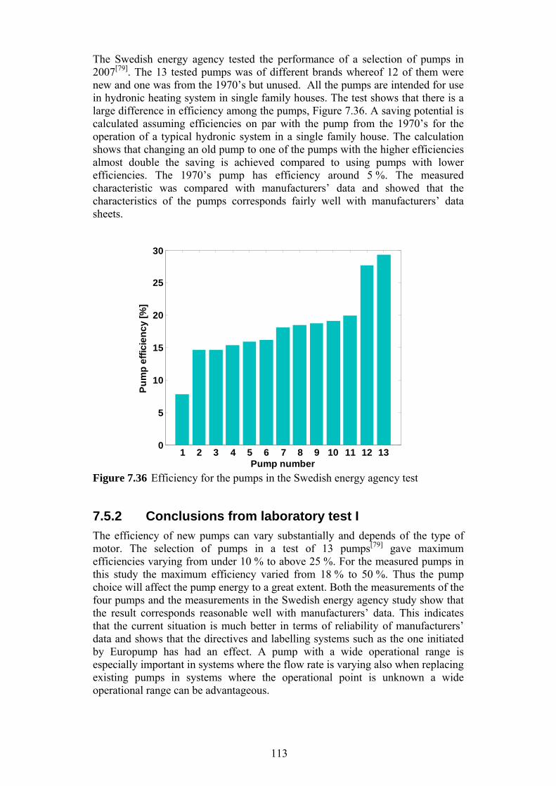
113

The Swedish energy agency tested the performance of a selection of pumps in 2007[79]. The 13 tested pumps was of different brands whereof 12 of them were new and one was from the 1970’s but unused. All the pumps are intended for use in hydronic heating system in single family houses. The test shows that there is a large difference in efficiency among the pumps, Figure 7.36. A saving potential is calculated assuming efficiencies on par with the pump from the 1970’s for the operation of a typical hydronic system in a single family house. The calculation shows that changing an old pump to one of the pumps with the higher efficiencies almost double the saving is achieved compared to using pumps with lower efficiencies. The 1970’s pump has efficiency around 5 %. The measured characteristic was compared with manufacturers’ data and showed that the characteristics of the pumps corresponds fairly well with manufacturers’ data sheets.

Figure 7.36 Efficiency for the pumps in the Swedish energy agency test

7.5.2 Conclusions from laboratory test I

The efficiency of new pumps can vary substantially and depends of the type of motor. The selection of pumps in a test of 13 pumps[79] gave maximum efficiencies varying from under 10 % to above 25 %. For the measured pumps in this study the maximum efficiency varied from 18 % to 50 %. Thus the pump choice will affect the pump energy to a great extent. Both the measurements of the four pumps and the measurements in the Swedish energy agency study show that the result corresponds reasonable well with manufacturers’ data. This indicates that the current situation is much better in terms of reliability of manufacturers’ data and shows that the directives and labelling systems such as the one initiated by Europump has had an effect. A pump with a wide operational range is especially important in systems where the flow rate is varying also when replacing existing pumps in systems where the operational point is unknown a wide operational range can be advantageous.

1 2 3 4 5 6 7 8 9 10 11 12 130

5

10

15

20

25

30

Pump number

Pu

mp

eff

icie

nc

y [

%]

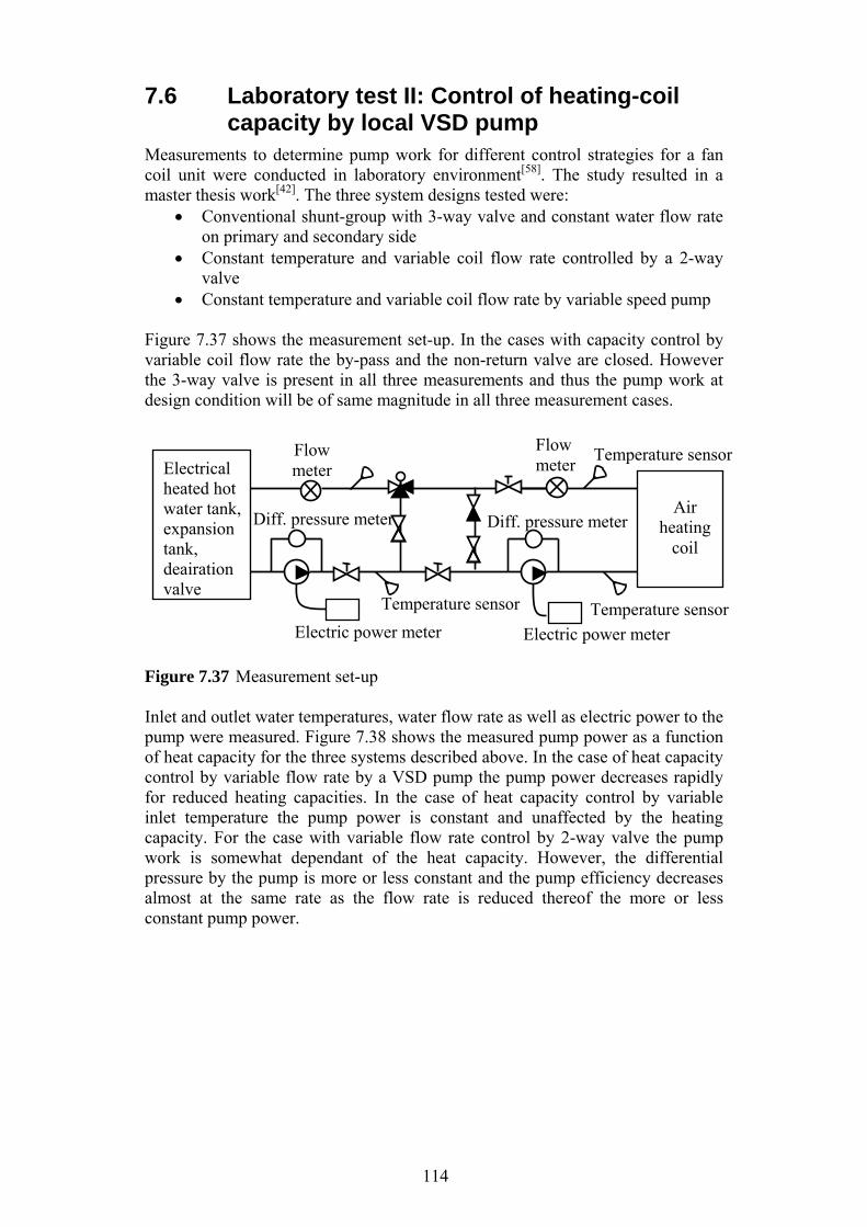
114

7.6 Laboratory test II: Control of heating-coil capacity by local VSD pump

Measurements to determine pump work for different control strategies for a fan coil unit were conducted in laboratory environment[58]. The study resulted in a master thesis work[42]. The three system designs tested were:

Conventional shunt-group with 3-way valve and constant water flow rate on primary and secondary side

Constant temperature and variable coil flow rate controlled by a 2-way valve

Constant temperature and variable coil flow rate by variable speed pump Figure 7.37 shows the measurement set-up. In the cases with capacity control by variable coil flow rate the by-pass and the non-return valve are closed. However the 3-way valve is present in all three measurements and thus the pump work at design condition will be of same magnitude in all three measurement cases.

Figure 7.37 Measurement set-up Inlet and outlet water temperatures, water flow rate as well as electric power to the pump were measured. Figure 7.38 shows the measured pump power as a function of heat capacity for the three systems described above. In the case of heat capacity control by variable flow rate by a VSD pump the pump power decreases rapidly for reduced heating capacities. In the case of heat capacity control by variable inlet temperature the pump power is constant and unaffected by the heating capacity. For the case with variable flow rate control by 2-way valve the pump work is somewhat dependant of the heat capacity. However, the differential pressure by the pump is more or less constant and the pump efficiency decreases almost at the same rate as the flow rate is reduced thereof the more or less constant pump power.

Electric power meter Electric power meter

Diff. pressure meter Air

heating coil

Electrical heated hot water tank, expansion tank, deairation valve

Flow meter

Flow meter

Temperature sensor Temperature sensor

Temperature sensor

Diff. pressure meter

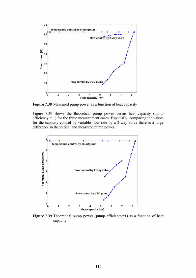
115

Figure 7.38 Measured pump power as a function of heat capacity Figure 7.39 shows the theoretical pump power versus heat capacity (pump efficiency = 1) for the three measurement cases. Especially, comparing the values for the capacity control by variable flow rate by a 2-way valve there is a large difference in theoretical and measured pump power.

Figure 7.39 Theoretical pump power (pump efficiency=1) as a function of heat

capacity

0 1 2 3 4 5 6 7 80

10

20

30

40

50

60

70

Heat capacity [kW]

Pu

mp

po

we

r [W

]

flow control by VSD pump

flow control by 2-way valve

temperature control by shuntgroup

0 1 2 3 4 5 6 7 80

1

2

3

4

5

6

Heat capacity [kW]

Th

eore

tic

al p

um

p p

ow

er [

W]

temperature control by shuntgroup

flow control by 2-way valve

flow control by VSD pump

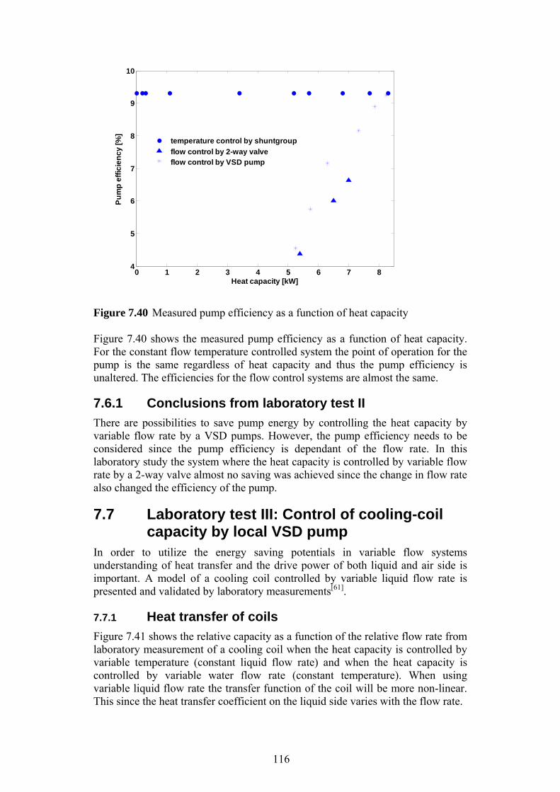
116

Figure 7.40 Measured pump efficiency as a function of heat capacity Figure 7.40 shows the measured pump efficiency as a function of heat capacity. For the constant flow temperature controlled system the point of operation for the pump is the same regardless of heat capacity and thus the pump efficiency is unaltered. The efficiencies for the flow control systems are almost the same.

7.6.1 Conclusions from laboratory test II

There are possibilities to save pump energy by controlling the heat capacity by variable flow rate by a VSD pumps. However, the pump efficiency needs to be considered since the pump efficiency is dependant of the flow rate. In this laboratory study the system where the heat capacity is controlled by variable flow rate by a 2-way valve almost no saving was achieved since the change in flow rate also changed the efficiency of the pump.

7.7 Laboratory test III: Control of cooling-coil capacity by local VSD pump

In order to utilize the energy saving potentials in variable flow systems understanding of heat transfer and the drive power of both liquid and air side is important. A model of a cooling coil controlled by variable liquid flow rate is presented and validated by laboratory measurements[61].

7.7.1 Heat transfer of coils

Figure 7.41 shows the relative capacity as a function of the relative flow rate from laboratory measurement of a cooling coil when the heat capacity is controlled by variable temperature (constant liquid flow rate) and when the heat capacity is controlled by variable water flow rate (constant temperature). When using variable liquid flow rate the transfer function of the coil will be more non-linear. This since the heat transfer coefficient on the liquid side varies with the flow rate.

0 1 2 3 4 5 6 7 84

5

6

7

8

9

10

Heat capacity [kW]

Pu

mp

eff

icie

nc

y [%

]

temperature control by shuntgroup

flow control by 2-way valveflow control by VSD pump

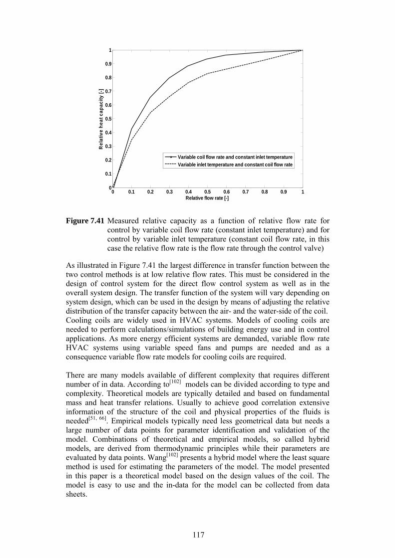
117

Figure 7.41 Measured relative capacity as a function of relative flow rate for control by variable coil flow rate (constant inlet temperature) and for control by variable inlet temperature (constant coil flow rate, in this case the relative flow rate is the flow rate through the control valve)

As illustrated in Figure 7.41 the largest difference in transfer function between the two control methods is at low relative flow rates. This must be considered in the design of control system for the direct flow control system as well as in the overall system design. The transfer function of the system will vary depending on system design, which can be used in the design by means of adjusting the relative distribution of the transfer capacity between the air- and the water-side of the coil. Cooling coils are widely used in HVAC systems. Models of cooling coils are needed to perform calculations/simulations of building energy use and in control applications. As more energy efficient systems are demanded, variable flow rate HVAC systems using variable speed fans and pumps are needed and as a consequence variable flow rate models for cooling coils are required. There are many models available of different complexity that requires different number of in data. According to[102] models can be divided according to type and complexity. Theoretical models are typically detailed and based on fundamental mass and heat transfer relations. Usually to achieve good correlation extensive information of the structure of the coil and physical properties of the fluids is needed[51, 66]. Empirical models typically need less geometrical data but needs a large number of data points for parameter identification and validation of the model. Combinations of theoretical and empirical models, so called hybrid models, are derived from thermodynamic principles while their parameters are evaluated by data points. Wang[102] presents a hybrid model where the least square method is used for estimating the parameters of the model. The model presented in this paper is a theoretical model based on the design values of the coil. The model is easy to use and the in-data for the model can be collected from data sheets.

0 0.1 0.2 0.3 0.4 0.5 0.6 0.7 0.8 0.9 10

0.1

0.2

0.3

0.4

0.5

0.6

0.7

0.8

0.9

1

Relative flow rate [-]

Re

lati

ve

he

at

ca

pa

cit

y [

-]

Variable coil flow rate and constant inlet temperature

Variable inlet temperature and constant coil flow rate

118

7.7.2 Heat transfer of coils - model

The model presented in this paper is intended for use in control applications and for modelling and simulation of energy use in buildings. The model is validated by measurement of two a cooling-coils where the capacity is controlled by variable liquid flow rate. The NTU method gives:

· · (7.18) By logarithmic differentiating[23, 30] equation (8.18), the sensitivity of the thermal capacity to changes in the respective parameter can be estimated (equation 7.19): ∆ ∆ ∆ ∆

(7.19)

Where ε=ε(R,NTU) is the effectiveness of the coil, / is the ratio of the minimum and maximum heat capacity flow rates, tb1 and tb2 is the inlet and return liquid temperatures respectively, ta1 and ta2 is the inlet and outlet air temperatures respectively. The temperature dependency of the density and the heat capacity is neglected as well as the heat resistance in the tube wall. The heat transfer coefficient on the liquid side is assumed to vary with the flow rate with an exponent m. Two non-dimensional control variables are introduced:

%

%

%

% (7.20)

where xb is the controlling variable and ya is the controlled variable.

7.7.2.1 Liquid flow rate control

The relation between the controlling variable xb (liquid flow ratio) and the controlled variable ya (coil capacity ratio) is given in equation 7.21-7.22[30].

[-] with (7.21)

[-] (7.22)

m is the flow related heat transfer exponent and is the liquid flow rate. The design constants Kd1 to Kd6 in the relations above are given by the ratio of heat transfer capacity on the liquid side to that of the air side (equation 7.723-7.24):

, · ,

, · , (7.23)

Air temperature change, i.e. required flow rate, at the design condition:

65

65

)(

1)(

dbdbb

bddba KxKxFx

xKKxFy

mbd

dmbb

xK

KxxF

1

1

1

1)(

db

bb

V

Vx

,

119

∆ , (7.24)

Liquid temperature change, i.e. required flow rate, at the design condition:

∆ , (7.25) Mean temperature difference, i.e. required heat exchanger size, at the design condition:

, (7.26) Constants introduced to simplify the relation for ya:

(7.27)

(7.28)

7.7.3 Model validation

Laboratory measurement of two cooling-coils of different sizes and geometries is used for validation of the model. For both coils the inlet and return water temperatures, the water flow rate as well as the inlet and outlet air temperatures and air flow rate is measured. The heat balance for the water and air side is calculated within 5 % of each other. The heat capacity is varied by a variable water flow rate. One of the cooling coils (coil 1) is situated in an in-line air handling unit. The design air flow rate is 1 m3/s and the design water flow rate is 0.74 litre/s. Cooling-coil 2 is a smaller coil situated in a room based fan-coil unit. The design air flow rate for coil 2 is 0.15 m3/s and the design water flow rate is 0.15 litre/s. For coil 2 two air flow rates are measured. Results are shown in Figure 7.42-7.43. The results show that the model fit reasonable well with the measurements throughout the measurement range. For medium flow rates the model predicts a slightly lower relative heat capacity. As seen in Figures 7.42-7.43 a relative flow rate of 30 % gives about 60-70 % of the heating capacity. The rapid increases in capacity with flow rate for small relative flow rates can make it difficult to control the heat capacity which increases the risk of on/off-behaviour of the coil or risk of control stability problems.

120

a)

b)

Figure 7.42 a) Relative capacity as a function of relative flow rate modelled and measured for cooling coil 1, b) relative modelled capacity as a function of relative measured capacity for cooling coil 1

0 0.1 0.2 0.3 0.4 0.5 0.6 0.7 0.8 0.9 10

0.1

0.2

0.3

0.4

0.5

0.6

0.7

0.8

0.9

1

Relative flow rate [-]

Re

lati

ve

he

at

ca

pa

cit

y [

-]

modeled

measured

0 0.1 0.2 0.3 0.4 0.5 0.6 0.7 0.8 0.9 10

0.1

0.2

0.3

0.4

0.5

0.6

0.7

0.8

0.9

1

Measured relative heat capacity [-]

Mo

de

led

re

lati

ve

he

at

ca

pa

cit

y [

-]

121

a)

b)

Figure 7.43 a) Relative capacity as a function of relative flow rate modelled and measured for cooling coil 2, b) relative modelled capacity as a function of relative measured capacity for cooling coil 2

7.7.4 Conclusion from laboratory test III

When controlling the liquid flow rate in air-coils the transfer function will be affected, and become more non-linear. When both the air side as well as the liquid side of the air coil has varied flow rates the heat transfer function must be considered, especially if one wants to minimize the energy used for both fans and pumps in combination. The non-linearity of the air-coil transfer function, giving 80% relative capacity at 30% relative flow, means that most of the theoretical reduction in pump power for the decentralized pump systems can be utilized.

0 0.1 0.2 0.3 0.4 0.5 0.6 0.7 0.8 0.9 10

0.1

0.2

0.3

0.4

0.5

0.6

0.7

0.8

0.9

1

Relative flow rate [-]

Re

lati

ve

he

at

ca

pa

cit

y [

-]

modeled 100 % air flow ratemeasured 100 % air flow rate

modeled 70 % air flow ratemeasured 70 % air flow rate

0 0.1 0.2 0.3 0.4 0.5 0.6 0.7 0.8 0.9 10

0.1

0.2

0.3

0.4

0.5

0.6

0.7

0.8

0.9

1

Measured relative heat capacity [-]

Mo

de

l re

lati

ve

he

at

ca

pa

cit

y [

-]

100% air flow rate

70% air flow rate

122

The aim of the model development is not to model one particular fan coil but to obtain a model that works in control context and for modelling/simulation of larger systems. Laboratory measurement of two air-coils was used to validate the model. Results show that the model fit reasonable well with the measurement. The rapid increases in capacity with relative flow rate up to 30 % can make it difficult to control the heat capacity which increases risk of on/off-behaviour of the coil or control stability problem.

123

8 Discussion, conclusions and future work

This thesis looks at the possibilities of improving the efficiency of building related pump and fan work. There are two main possibilities:

Higher component efficiency of circulators, motors and drives.

Lower pressure drop by means of new components (filters, heat exchangers etc.) but primarily by new system design.

The first alternative can provide savings directly by simply exchanging an existing circulator with a new and more efficient. The second alternative requires major rethinking regarding system design and control but also provides the most far-reaching advantages. This chapter provides a summarized discussion and consequences of these alternatives and the findings in relation to this work.

8.1 Discussion A way of illustrating the system efficiency of fan and pump systems is the use of SFP and SPP. These goodness numbers are determined by the total fan/pump efficiency and the total pressure difference. Often both factors have to be addressed. For instance, assuming that a fan efficiency of a system is improved from 60 % to 70 %, the SFP is reduced by only 14 %. To be able to meet the national energy target of an energy reduction by 50 % until 2050 the fan system design and system pressure drops must be considered. The SFP is proportional to the system pressure drop and a reduction of this pressure drop by 50 % is not easily achieved. In general it will require new system designs.

8.1.1 Present situation

The current pump and fan operation in Swedish non-industrial buildings has been investigated by available statistics and information. The investigation gave a fairly good overview of the use of pumps and fans in commercial, public and residential buildings. However, more detailed information is lacking at component level and, as a consequence, in some cases assumptions regarding sizes and efficiencies had to be made. To be able to estimate the saving potential when changing current pumps and fans to more efficient units, assumptions regarding efficiencies had to be made. Assumptions made are based on current regulations [90] and manufacturers’ data. The calculated technical saving potential for pump and fan operation in non-industrial buildings by means of improved pump efficiency and specific fan power is 50 % and 40 % respectively.

8.1.2 System design

Pressure drops in air and liquid systems consist to a great extent of pressure drop for valves and dampers that direct and quantify the flow rate in the system. By removing these dampers and valves and replacing them by decentralized variable speed pumps and fans the system pressure drop can be reduced substantially. The theoretical saving potential in using decentralized pump and fan systems is indisputable since pressure drop devices as valves and dampers are removed. However, since small circulators generally have lower efficiency than large

124

circulators the real saving potential will be affected by the circulator efficiency. The biggest potential for improvement lies in motor and motor drive developments. The induction motor is currently the most commonly used motor in HVAC applications. Permanent magnet motors with frequency converters are becoming more frequently used. Generally permanent magnet motors have higher efficiency and a wider working range compared to the induction motor. It is to a great extent the availability of these motors and frequency converters that makes alternative system designs such as decentralized systems possible.

8.1.3 Case studies

The thesis contains four case studies. In case study I the electrical power to a radiator pump was measured for a heating season. With the measured electrical power and the use of a simple pump model the flow rate for the whole measurement period could be calculated. A limitation of the model was the inability of calculating the pump efficiency. The model could be used to evaluate the operational times and capacities of the system. One observation in this study was that the heating capacity for the system never reached the design heating capacity, which is believed to be true for pump systems in general. The case study also highlights the obvious importance of choice of inlet temperature. With too high an inlet temperature, and a correspondingly low flow rate, the heat may never enter the room/zone as intended but instead be lost on the way. The conclusion from this case study is that both heat and pump energy must be taken into account when designing decentralized pump systems. In case study II a radiator system is rebuilt from a temperature controlled system to a decentralized direct flow control system. The results from the case study showed a saving potential in pump energy of about 70 %. In this case study temperature setback was used under non-working hours and results showed a heat energy saving of 50 % during the measurement period. In order for temperature setback to be effective it has to contribute to a decrease in the average temperature of the building. The temperature set-back was used only for the top floor of the building and obviously heat will flow from the floor beneath. This was unfortunately not foreseen. The room temperature of the floor beneath as well as the total heat energy should have been measured. As a consequence the saving potential had to be recalculated instead of measured. In case study III the temperature efficiency of two enthalpy wheels and two run-around-loops was examined with a fan and pump energy perspective. Higher temperature efficiency can come at the expense of increased fan energy. The result showed that for both the enthalpy wheel and the run-around-loop the heat recovery with lower temperature efficiency was to prefer. The primary energy ratio and the energy cost ratio of heat and electricity will enhance the importance of minimizing fan and pump power. In case study IV two air-handling units were investigated with focus on the air heating and air cooling coils. For the air heaters and air coolers the operational times were low and full heating/cooling capacities were never used. A system design with air-cooler and air-heater situated in parallel with the AHU or a system design where the heating or cooling need is solved locally would certainly save

125

fan energy in this case. The air heaters and air coolers constitute 12 % and 17 % of the total pressure drop for AHU 1 and AHU 2 respectively.

8.1.4 Laboratory investigations

In addition to the case studies, the thesis also contains three laboratory investigations In laboratory test I the efficiency of four pumps was measured. When choosing a pump it is important to know that the pump performs as expected. Also the efficiency of pumps can vary substantially and depends of the type of motor. For the measured pumps in this study the maximum efficiency varied from 18 % to 50 %. Thus the pump choice will affect the pump energy to a great extent. The measurements of the four pumps show that the results correspond fairly well with manufacturers’ data. A limitation of this study is that the pump efficiency was not measured for several fixed speeds which would give information of how the speed affects the efficiency of the pump. This would have given valuable information that could be used for validation of models. In laboratory test II the pump power was measured for three different strategies for capacity control of a fan-coil unit; temperature control by a shunt group with constant flow rate, variable flow rate control by a two-way valve and direct flow rate control by a variable speed pump. In the system where the heat capacity is controlled by variable flow rate using a 2-way valve, almost no saving was achieved compared to the temperature controlled system. This relates to the pump efficiency being reduced with decreasing flow rate. The measurement set-up did not allow for the right amount of reduction of pressure drop at design condition for the direct flow control by variable speed pump. Also the same pump was used for all three control strategies in spite of the different design conditions. In laboratory test III the characteristics of two cooling air-coils were measured when controlling the cooling capacity with direct flow control. When controlling the liquid flow rate in air-coils the transfer function will be affected and become more non-linear. When both the air side as well as the liquid side of the air coil have varied flow rates the heat transfer function must be considered, especially if one wants to minimize the energy used for both fans and pumps in combination. A model of the heat transfer function was validated by the measurements. The aim of the model is not to model one particular fan coil but to obtain a model that works in a control context and for modelling/simulation of larger systems. Results show that the model agreed reasonably well with the measurements even though laminar flow is obtained for a relative flow rate of about 30 % in both cases. The measurements were made during winter time with correspondingly dry air and thus no condensation on the coil surfaces occurred. For this reason the influence of condensation is not implemented in the model at this stage.

8.2 Conclusion In this thesis the possibility of using decentralised fan and pump systems in order to reduce fan and pump energy has been investigated. Reduced loads and limited time of operation as well as low occupancy levels indicate that there is a large saving potential when using demand control fan- and pump operation for Swedish buildings.

126

8.2.1 Air systems

The saving potential in fan energy for Swedish non-industrial building is estimated to 40 % by improving SFP to recommended values. For further reduction of SFP the improvement in fan efficiency is not enough and the system pressure drop must be targeted. Parallel or locally situated air-heater and air-coolers can reduce the system pressure drop by about 10-20 % leading to a 10-20 % reduction in SFP.

8.2.2 Liquid systems

By improving pump efficiency the overall energy saving for pump operation in non-industrial buildings in Sweden is estimated to 50 %. The large difference in saving potential between pumps and fans is due to the current situation of pumps in buildings generally having quite low efficiencies, in some cases below 5 %. Fans, in comparison, show efficiencies that may exceed 60 %. In real numbers the saving in pump operation is on the same level as for fan operation. Adding to the savings by new pumps, system changes can give further savings by pump operation. A proposed decentralized pump system has been implemented in real life and results shows a reduction of pump energy by as much as 70 %. In this system, temperature set-back was used for non-working hours resulting in a heat energy saving of 50 %. The system investigated is a commercial system developed recently which proves that decentralized pump systems are interesting even when cost is taken into account.

8.2.3 Motors and drives

To be able to reduce fan and pump energy beyond the component level improvements, different system solution must be considered. With variable speed drives available even for small motors energy costly devices such as dampers and valves can be removed and replaced by direct flow control by VSD pumps and fans. In these systems it is important to use components that have motors and motor drives which can handle quadratic loads at low load levels.

8.2.4 Objectives and results

The objective of this thesis was to find means to reduce pump and fan energy in Swedish non-industrial buildings. The aim was to find components and system designs that can provide energy reduction in pump and fan systems by 50 %. For pump systems saving potentials above 50 % have been shown both by measurements and by modelling for decentralized systems. The efficiency of pumps has increased substantially with the use of permanent magnet motors and offers the targeted energy saving potential alone. To be able to fulfil the energy reduction target for fan systems, several combined actions might be needed, as reducing pressure drop and increasing fan efficiency. Decentralized systems, where the conditioning of air is solved locally on a demand basis, might be a solution. The investigation of alternative system designs for air systems and the corresponding saving potential has not been examined to the extent wished. However, a clear saving potential has been identified.

127

8.3 Future work Some suggestions for future work are:

Investigations of decentralized pump systems in multi-family buildings, mainly concentrated on practical and costs aspects, particularly in refurbishment situations.

Investigate possibilities for combination of decentralized pump system and heat source (for example heat pump) to optimize system efficiency.

Investigate local demand control hydronic heating and cooling systems, mainly decentralized system with room-based heating/cooling coils etc. An aspect for room based system is noise generated by decentralized fans.

Investigate parallel air handling unit with respect to pressure drops, space requirements compared to traditional in-line air handling units, possibilities to use high efficient axial fans (as pressure drops in the systems are considerable lower), noise levels, economy.

128

129

References 1. Motor list (Swedish energy agency.)

http://energimyndigheten.se/sv/Foretag/Energieffektivisering-i-foretag/Tillverkningsindustri---hjalpsystem-och-processer/Elmotorer/.

2. Test of exhaust fans intended for 85 m2, 130 m2 and 190 m2 heated floor

area. Accessed 28th Sep 2011, (Swedish energy agency.) http://www.energimyndigheten.se/sv/Hushall/Testerresultat/Testresultat/Franluftsflaktar-for-hus-med-omkring-85m-boyta/?tab=2.

3. Andersen, H P, 2005. Europeans agree on energy standards for pumps.

News from DBDH, no. 3, Fredriksberg, Danmark. 4. Andreasson, M, Borgström, M, Werner, S, 2008. Värmeanvändning i

flerbostadshus och lokaler 2006, En djupare analys av SCB:s underlagsmaterial till den svenska energistatistiken för byggnader.

5. ASHRAE standard 90.1-2010, 2010. (American Society of Heating,

Refrigerating and Air-Conditioning Engineers.) Atlanta. 6. Bernier, M A, Bourret, B, 1999. Pumping energy and variable frequency

drives. ASHRAE Journal, vol. 41, no. 12, December, pp. 37-40. (Amer. Soc. Heating, Ref. Air-Conditoning Eng. Inc.) Atlanta.

7. Bidstrup, N, Hunnekuhl, H, Heinrich, T, Andersen, T, 2003. Classification

of Circulators. (Europump.). 8. Børresen, B, 1994. Konstant trykk over pumpe er ikke nok. Norsk VVS,

no. 14, Norway. 9. Børresen, B, 1994. Mengderegulering - et energiriktig

dimensjoneringskonsept. Norsk VVS, no. 11, pp. 21-27. Norway. 10. Carlson, R, 2000. Correct method of calculating energy savings to justify

adjustable-frequency drives on pumps. IEEE Transactions on Industry Applications, vol. v 36, no. n 6, Nov, pp. p 1725-1733. (Institute of Electrical and Electronics Engineers Inc.) Piscataway, NJ, USA.

11. COMMISSION REGULATION (EU) No 327/2011 of 30 March 2011-

implementing Directive 2009/125/EC, 2011. 12. de Almeida, Fonseca, Bertoldi, 2003. Energy-efficient motor systems in

the industrial and in the services sectors in the European Union: Characterisation, potentials, barriers and policies. Energy, vol. 28 no. 7, June, pp. 673-690 (Elsevier.) Oxford.

13. de Almeida, Fonseca, Falkner, Bertoldi, 2003. Market transformation of

energy-efficient motor technologies in the EU. Energy Policy, vol. 31 no. 6, May, pp. 563-575 (Elsevier.) Oxford.

130

14. de Almeida, Ferreira, Both, 2005. Technical and economical

considerations in the application of variable-speed drives with electric motor systems. IEEE Transactions on Industry Applications, vol. 41, no. 1, January, pp. 188-199. (Institute of Electrical and Electronics Engineers.) New York.

15. Dieckmann, J, Brodrick, J, 2010. VFDs for chiller auxiliaries. ASHRAE

Journal, July, pp. 96-99. (American Society of Heating, Refrigeration and Air-conditioning Engineers.) Atlanta.

16. DIRECTIVE 2006/32/EC, 2006. Official Journal of the European Union. 17. Ecodesign, 2009. Directive 2005/32/EC. 18. Energiläget 2007, 2007. (Swedish energy agency.) Eskilstuna. 19. Energiläget 2010, 2010. (Swedish energy agency.) Eskilstuna. 20. Eurovent Certification, 2009-04-01. (Presentation at project Meeting:

www.eurovent-certification.com/, 21. Everhart, J, Sanchez, K, 2004. 'Sensing' significant savings with VFD

systems. World Pumps, vol. 2004, no. 450, March, pp. 18-21. (Elsevier Ltd.) Kent.

22. Fahlén, P, 1994. Performance test of air source heat pumps under frosting

conditions - Quality of Results. SP report 1994:01, pp. 328. (Swedish National Testing and Research Institute.) Borås.

23. Fahlén, P, Voll, H, Naumov, J, 2006. Efficiency of pump operation in

hydronic heating and cooling systems. Journal of Civil Engineering and Management vol. 12, no. 1, March, pp. 57-62. (Lidykla Technika.) Vilnius, Litauen.

24. Fahlén, P, 2007. Capacity control of air coils in sytsems for heating and

cooling-transfer function and drive power. (Chalmers university of technology.) Gothenburg, Sweden.

25. Fahlén, P, 2009. Kvalitetsdeklaration av mät- och beräkningsresultat. pp.

32. (Avdelningen för Installationsteknik, Chalmers tekniska högskola.) Göteborg.

26. Fahlén P, Prof. Building services engineering, Chalmers university of

technology. 27. Fahlén P., 2007. Compendium K2007:01 Heating Ventilation and Air

Conditioning (HVAC) Systems Engineering - Appendix 1 System of units, designations, symbols, abbreviations and definitions. Göteborg.

131

28. Fahlén P., Markusson C., Haglund Stignor C., 2007. Capacity Control of Liquid-cooled air-coolers. International Congress of Refrigeration, Beijing, Aug.

29. Fahlén P., Markusson C., Maripuu M-L., 2007. Opportunities in the design

of control-on-demand HVAC system. Clima 2007 WellBeing Indoors, Helsinki, June. (FINVAC ry.)

30. Fahlén P., 2009. Capacity control of hydronic fan coil units reduction of

pump work. (Chalmers University of Technology.) Gothenburg. 31. Fahlén P., Markusson C., 2011. Capacity control of air coils for heating

and cooling - Transfer functions, drive power and system design. Ashrae winter conferecne, Las Vegas,

32. Falkner, H, 2008. EUP Lot 11: Circulators in buildings. Report to the

European Commission. . 33. Glover, A, 2005. Oversizing pump motors - The problems. World Pumps,

no. 466, July pp. 36-38 (Elsevier.) Surrey. 34. Göransson, A, Lindahl, U, Forsman, G, Hedenström, C, 1992. STIL-

studien 2000, Lokalerna och energihushållningen. pp. 164. (Vattenfall.) Vällingby.

35. Göransson, A, 2008. Energianvändning och bebyggelse 2003, bilaga till

Boverkets utredning om styrmedel om energieffektivisering i byggnader-Piska och morot. (Boverket.) Karlskrona.

36. Hallén, T, 1981. Mathematical expression for the duration of outdoor air

temperature (in Swedish). VVS-special Värmeåtervinning, pp. 57-58. 37. Hartman, T, 2001. Ultra-efficient cooling with demand-based control.

HPAC Heating/Piping/Air conditioning Engineering, Dec. 38. Hydraulic Institute, Europump, Department of Energy, 2004. Variable

speed pumping A guide to successful applications, Executive summary. pp. 15.

39. Ionel, D, 2010. High-efficiency variable-speed electric motor drive

techmologies for energy savings in the US residential sector. 12th international conference on optimization of electrical and electronic equipment, OPTIM 2010.

40. Jagemar, L, 1996. Design of energy efficient buildings. pp. 237. (Chalmers

University och Technology.) Göteborg. 41. Jagemar L, Ass. Prof. Building services engineering, Chalmers university

of technology.

132

42. Jahani A.K., 2007. Pumparbete samt returtemperatur för tre alternativa lösningar vid koppling till luftvärmare. pp. 47. (Chalmers tekniska högskola.) Göteborg.

43. Jensen, L, 1983. Nattsänkning av temperatur i flerbostadshus. (Statens råd

för byggforskning.) Stockholm. 44. Johansson, K, Matsson, J, 2011. (Energy and Environment.). 45. Karassik, I, Messina, J, Cooper, P, Heald, C, 2001. Pump Handbook. Ed.

Third, (McGraw-Hill.) USA. 46. Kays, W M, London, A L, 1984. Compact heat exchangers. (McGraw-

Hill Book Company.) New York. 47. Keulenaer, H, 2004. Energy efficient motor driven systems. Energy and

environment vol. 15, no. 5, (Multi-science publishing company.) UK. 48. Kristiansson, D, 2000. Cirkulationspumpar med varvtalsreglering Energi

& Miljö, no. 11, pp. 1-2. Stockholm. 49. Lelkes, A, Krotsch, J, De Doncker, R W, 2002. Industry Applications

Conference 37th IAS Annual Meeting, vol. 3, Oct, pp. 2036-2042. USA. 50. Lelkes, A, Bufe, M, 22004. BLDC motor for fan application with

automatically optimized commutation angle. Power Electronics Specialists Conference, PESC 04. IEEE 35th Annual,

51. Li P, L Y, Seem J., 2010. Modelica-Based Dynamic Modeling of a

Chilled-Water Cooling Coil. HVAC&R Research, vol. 16(1), pp. 35-58. 52. Lizardos, E, Elovitz, K, 2000. Damper Sizing Using Damper Authority.

ASHRAE Journal, vol. 42, no. 4, April, pp. 37-38+40+42+44+46 (American Society of Heating, Refrigerating and Air-Conditioning Engineers.) Atlanta.

53. Ma, Z, Wang, S, 2009. Energy efficient control of variable speed pumps in

complex building central air-conditioning systems. Energy and Buildings, vol. 41, no. 2, February, pp. 197-205.

54. Maripuu, M-L, 2006. Adapting Variable Air Volume (VAV) Systems for

Office Buildings without Active Control Dampers. pp. 131. (Chalmers University of Technology.) Göteborg.

55. Maripuu, M-L, Jagemar, L, 2007. Design criteria for variable air volume

(VAV) systems without active control dampers. International congress of refrigeration, Aug, Beijing.

56. Maripuu, M-L, 2009. Demand control ventilation systems in commercial

buildings. (Building servicees engineering, Chalmers university of technology.) Gothenburg.

133

57. Markusson, C, 2009. Effektivisering av pump och fläktdrifter i byggnader.

(Energy and environment, Chalmers university of technology.) Göteborg, Sweden.

58. Markusson C, Jagemar L, Fahlén P, 2010. Energy recovery in air handling

systems in non-residential buildings - design considerations. The 2010 ASHRAE Annual Conference, Albuquerque, USA, ASCHRAE.)

59. Markusson C, Åström J, Jagemar L, Fahlén P, 2010. Electricity use and

efficiency potential of pump and fan operation in buildings. CLIMA 2010, Antalya, Turkey, 10th REHVA World congress.)

60. Markusson C, Jagemar L, Fahlén P, 2011. System design for energy

efficient pump operation in buildings. eceee 2011 Summer Study, Giens, France,

61. Markusson C, Jagemar L, Fahlén P, 2011. Capacity control of air-coils-

drive power, system design and modeling of variable liquid flow air coil. The 23rd IIR International Congress of Refridgeration, Prague, Check Republic,

62. Martin, J, 2008. Energy savings from inverter drives in the efficient

building. World Pumps, vol. 2008 no. 498, March, pp. 32-34 (Elsevier.) Surrey

63. Mescher, K, 2009. Simplified GCHP system. ASHRAE Journal, October,

pp. 24-40. (American society for heating, refrigeration and air-conditioning engineering.) Atlants.

64. Meyer, F, 2006. Dezentrale Heizungspumpen. Bine Projekinfo, no. 13, pp.

1-4. Eggenstein-Leopoldshafen. 65. Mora, J L V, Lelkes, A, Pacas, J M, 2002. External rotor PM motor fed by

a load commutated inverter for fan applications. Industrial Electronics Society, IEEE 2002 28th Annual Conference, 5-8 Nov. (

66. Morisot O, M, D, Stabat P, 2002. Simplified Model for the Operation of

Chilled Water Cooling Coils Under Nonnominal Conditions. HVAC&R Research vol. 8(2), pp. 135-156.

67. Nilsson, P E, 2003. Achieving the Desired Indoor Climate.

(Studentlitteratur.) Lund. 68. Nyman, B, 2004. Energideklarering av byggnader - för effektivare

energianvändning. SOU 2004:109, (Sveriges offentliga utredningar.) Stockholm.

69. Osborn, K G, 2005. Fan data: Is what you see, what you get? ASHRAE

Journal, vol. 47, no. 11, November pp. 24-29. (American Society of Heating, Refrigerating and Air Conditioning Engineers.) Atlanta.

134

70. Paarporn, S, 2000. Local pumping system. ASHRAE Journal, vol. 42, no.

9, September, pp. 26-28+30-32. (Amer. Soc. Heating, Ref. Air-Conditoning Eng. Inc.) Atlanta.

71. Petitjean, R, 2002. Injustering av radiator system. (Tour and Andersson.)

Sweden. 72. Petitjean Robert, 1995. Total Injustering. (Tour & Andersson Hydronics

AB.) Sverige. 73. Projekt BETSI, 2009. Hur mår husen? (Boverket.) Karlskrona. 74. Rishel, J B, 2001. Wire-to-water efficiency of pumping systems.

ASHRAE Journal, vol. 43, no. 4, April, pp. 40+42+44-46. (Amer. Soc. Heating, Ref. Air-Conditoning Eng. Inc.) Atlanta.

75. Rishel, J B, 2003. Control of variable speed pumps for HVAC water

systems. ASHRAE Winter Meetings Cd Technical and Symposium Chicago, IL, United States, Jan 26-29. (Amer. Soc. Heating, Ref. Air-Conditoning Eng. Inc.)

76. Rishel, J B, 2010. Wire-to-shaft efficiency. ASHRAE Journal, July,

(American society of heating, refrigeration and air-conditioning engineering.) Atlanta.

77. Roth, K W, Dieckmann, J, Brodrick, J, 2003. Demand control ventilation.

ASHRAE Journal, vol. 47, no. 5, July, pp. 91-92. (American Society of Heating, Refrigerating and Air Conditioning Engineers.) Atlanta.

78. Roth, K W, Chertok, A, Dieckmann, J, Brodrick, J, 2004. Electronically

commutated permanent magnet motors. ASHRAE Journal, vol. 46, no. 3, March, pp. 75-76. (Amer. Soc. Heating, Ref. Air-Conditoning Eng. Inc.) Atlanta.

79. Ruud, S, 2007. Provning av cirkulationspumpar. P6 04289, pp. 7. (SP

Sveriges Tekniska Forskningsinstitut.) Borås. 80. Sahlin K, Stengård L, 2011. Energy statistics for one and two-dwelling

buildings in 2009. (Swedish energy agency.) Eskilstuna. 81. Sahlin K, Stengård L, 2011. Summary of energy statistics for dwellings

and non-residential premises for 2009. (Statens energimyndighet.) Eskilstuna.

82. Sahlin K, Stengård L, 2011. Energy statistics for non-residentional

premises in 2009. (Swedish energy agency.) Eskilstuna. 83. Sinnesbichler H., Schade A., Eberl M., 2010. Vergleich einer

konventionellen Heizungsanlage mit dem Decentralen Pumpensystem

135

Wilo-Geniax. (Kurzfassung: Abschlossbericht Fraunhofer-Institut für Bauphysik.) Valley.

84. Statens energimyndighet, 2006. Förbättrad energistatistik för lokaler -

”Stegvis STIL” Rapport för år 1 Inventeringar av kontor och förvaltningsbyggnader. ER 2007:34, (Statens energimyndighet.) Eskilstuna.

85. Statens energimyndighet, 2007. Energianvändning & innemiljö i skolor

och förskolor - Förbättrad statistik i lokaler, STIL2. ER 2007:11, (Statens energimyndighet.) Eskilstuna.

86. Statens energimyndighet, 2008. Energianvändning i vårdlokaler -

Förbättrad statistik för lokaler, STIL 2. ER 2008:09, (Statens energimyndighet.) Eskilstuna.

87. Statens energimyndighet, 2009. Energianvändning i idrottsanläggningar -

Förbättrad statistik för lokaler, STIL2. ER 2009:10, (Statens energimyndighet.) Eskilstuna.

88. Statistics Sweden, 2011. English Kalkylerat bostadsbestånd 2010-12-31.

Örebro. 89. Stein, J, Zhou, A, Hwakong, C, 2007. Advanced variable air volume

system design guide. pp. 316. (California Energy Commission’s Public Interest Energy Research (PIER).) USA.

90. Swedish building code BBR, 2008. (Boverket.) Karlskrona, Sweden. 91. Swedish energy agency, 2006. Förbättrad energistatistik för lokaler -

”Stegvis STIL” Rapport för år 1 Inventeringar av kontor och förvaltningsbyggnader. ER 2007:34, (Statens energimyndighet.) Eskilstuna.

92. Swedish energy agency, 2007. Energianvändning & innemiljö i skolor och

förskolor - Förbättrad statistik i lokaler, STIL2. ER 2007:11, (Statens energimyndighet.) Eskilstuna.

93. Swedish energy agency, 2008. Energianvändning i vårdlokaler -

Förbättrad statistik för lokaler, STIL 2. ER 2008:09, (Statens energimyndighet.) Eskilstuna.

94. Swedish energy agency, 2009. Energianvändning i idrottsanläggningar -

Förbättrad statistik för lokaler, STIL2. ER 2009:10, (Statens energimyndighet.) Eskilstuna.

95. Swedish energy agency, 2011. Förbättrad statistik för lokaler, STIL2,

Energianvändning i hotell, restauranger och samlingslokaler. (Statens energimyndighet.) Eskilstuna.

136

96. Taylor, S T, 2002. Primary-only vs. primary-secondary variable flow systems. ASHRAE Journal, vol. 44, no. 2, February, pp. 25-29. (American society of heating, refrigeration, air-conditioning engineering.) Atlanta.

97. Taylor, S T, 2007. Increasing efficiency with VAV system static pressure

setpoint reset. ASHRAE Journal, vol. 49, no. 6, June, pp. 24-32 (American Society of Heating, Refrigerating and Air Conditioning Engineers.) Atlanta.

98. The Motor Challenge Programme, 2009-04-01. (Presentation at project

Meeting: http://re.jrc.ec.europa.eu/energyefficiency/motorchallenge/tools.htm,

99. Tolstoy, N, Borgström, M, Högberg, H, Nilsson, J, 1993.

Bostadsbeståndets tekniska egenskaper ELIB-rapport nr 6. pp. 104. (Statens institut för byggnadsforskning.) Gävle.

100. Trüschel, A, 2005. The value of balancing of hydronic systems, (in

Swedish). (Svensk Fjärrvärme AB.). 101. UKAS, 1997. The Expression of Uncertainty and Confidence in

Measurement. Ed. 1, pp. 76. (United Kingdom Accreditation Service.) England.

102. Wang Y-W, C W-J, Soh Y-C, Li S-J, Lu L, Xie L., 2004. A simplified

modeling of cooling coils for control and optimization of HVAC systems, . Energy Conversion and Management, vol. 45, pp. 2915-2930.

103. Veness, J, 2007. Improving efficiency through system-based changes.

World Pumps, vol. 2007, no. 494, November, pp. 32-34 Kent. 104. Wulfinghoff, D, 2011. Multiple-sone HVAC An obsolete template. Energy

Engineering, pp. 44. (Taylor and Francis Ltd.) London. 105. VVS-Tekniska föreningen, 1974. VVS-handboken Tabeller och Diagram.

(Förlags AB VVS.) Stockholm. 106. Åström, J, 2011. Investigation of Issues related to electrical efficiency

improvments of pump and fan drives in buildings (Department of Energy and environment, Chalmers university of technology.) Gothenburg.

107. Åström J, 2008. Division of electric power engineering, Department of

Energy and Environment, (Chalmers University of Technology ) Göteborg.

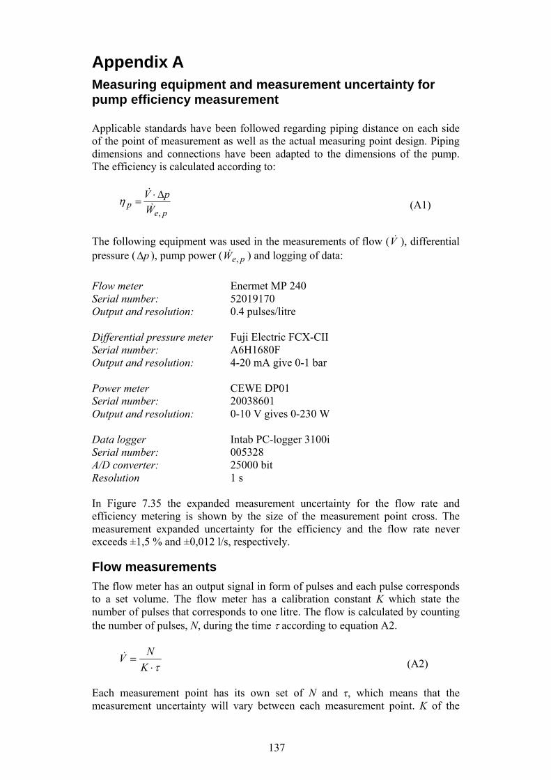
137

Appendix A Measuring equipment and measurement uncertainty for pump efficiency measurement Applicable standards have been followed regarding piping distance on each side of the point of measurement as well as the actual measuring point design. Piping dimensions and connections have been adapted to the dimensions of the pump. The efficiency is calculated according to:

pep W

pV

,

(A1)

The following equipment was used in the measurements of flow (V ), differential pressure ( p ), pump power ( peW ,

) and logging of data:

Flow meter Enermet MP 240 Serial number: 52019170 Output and resolution: 0.4 pulses/litre Differential pressure meter Fuji Electric FCX-CII Serial number: A6H1680F Output and resolution: 4-20 mA give 0-1 bar Power meter CEWE DP01 Serial number: 20038601 Output and resolution: 0-10 V gives 0-230 W Data logger Intab PC-logger 3100i Serial number: 005328 A/D converter: 25000 bit Resolution 1 s In Figure 7.35 the expanded measurement uncertainty for the flow rate and efficiency metering is shown by the size of the measurement point cross. The measurement expanded uncertainty for the efficiency and the flow rate never exceeds ±1,5 % and ±0,012 l/s, respectively.

Flow measurements

The flow meter has an output signal in form of pulses and each pulse corresponds to a set volume. The flow meter has a calibration constant K which state the number of pulses that corresponds to one litre. The flow is calculated by counting the number of pulses, N, during the time according to equation A2.

K

NV

(A2)

Each measurement point has its own set of N and τ, which means that the measurement uncertainty will vary between each measurement point. K of the

138

flow meter is 0.4 pulses/litre and the time resolution for the logger is 1s. The number of pulses and the measurement time will affect the combined uncertainty. The measurement uncertainty is calculated by differentiating equation A3 [25, 101].

K

K

N

N

V

V

(A3)

The judgement of the measurement uncertainty is considering contributions from calibration, measurement reading, installation, and operation conditions. According to the calibration record the flow meter has different measurement errors for different flow ranges, Table A1. Table A1 Flow meter calibration record Quantity

minV (minimum flow)

tV

(flow range border)

nV

(nominal flow)

Flow [l/s] 0.01 0.07 1.1 Error [%] 1.29 -0.01 -0.61 As the minimum is 0.4 l/s the uncertainty is approximated to ±1 % for the whole measured flow range. This is a simplification but a also an overestimation of the uncertainty compared to if individual calibration corrections had been made for each measurement point. The estimated uncertainty component will be neglected, i.e.

KuA 100

01 pulses/litre (A4)

The expected uncertainty, assuming uniform probability distribution is:

Ka

uB 100

6,0

31 pulses/litre (A5)

The flow meter readings include pulse counting and time readings. Pulse counting over a given time gives a mean value of the flow during the time interval and the estimated uncertainty is neglected, i.e. 02 Au pulses. The reading uncertainty is ±1 and thus the half width of the interval a = ±1 pulse. The expected measurement uncertainty, assuming uniform probability distribution is:

603

2 ,a

uB pulses (A6)

The time readings are done using the logger clock. The estimated uncertainty is neglected, i.e. 03 Au s.

The uncertainty assigned to the reading is assigned to ±1 second. Thus the half width of the interval a = ±1 s. The expected measurement uncertainty, assuming uniform probability distribution is:

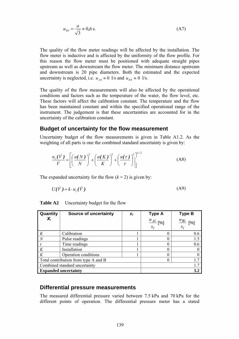
139

603

3 ,a

uB s. (A7)

The quality of the flow meter readings will be affected by the installation. The flow meter is inductive and is affected by the uniformity of the flow profile. For this reason the flow meter must be positioned with adequate straight pipes upstream as well as downstream the flow meter. The minimum distance upstream and downstream is 20 pipe diameters. Both the estimated and the expected uncertainty is neglected, i.e. 04 Au l/s and 04 Bu l/s. The quality of the flow measurements will also be affected by the operational conditions and factors such as the temperature of the water, the flow level, etc. These factors will affect the calibration constant. The temperature and the flow has been maintained constant and within the specified operational range of the instrument. The judgement is that these uncertainties are accounted for in the uncertainty of the calibration constant.

Budget of uncertainty for the flow measurement

Uncertainty budget of the flow measurements is given in Table A1.2. As the weighting of all parts is one the combined standard uncertainty is given by: 21222 /

)()()()(

u

K

Ku

N

Nu

V

Vuc

(A8)

The expanded uncertainty for the flow (k = 2) is given by: )()( VukVU c

(A9)

Table A2 Uncertainty budget for the flow

Quantity Xi

Source of uncertainty ci Type A

i

Ai

x

u[%]

Type B

i

Bi

x

u [%]

K Calibration 1 0 0.6N Pulse readings 1 0 1.5τ Time readings 1 0 0.6K Installation 1 0 0K Operation conditions 1 0 0Total contribution from type A and B 0 1.7Combined standard uncertainty 1.7Expanded uncertainty 3.2

Differential pressure measurements

The measured differential pressure varied between 7.5 kPa and 70 kPa for the different points of operation. The differential pressure meter has a stated

140

uncertainty of ±0.13 kPa. The estimated uncertainty is neglected. i.e. 05 Au kPa.

The expected uncertainty assuming uniform probability distribution is:

3

130

35

,

auB kPa (A10)

The reading of the differential pressure is a mean value throughout the measurement period. In pressure measurements the positioning and design of the pressure nipples is important. The nipples should be placed perpendicular to the flow and designed in a way that disturbances of the flow are minimized. Applicable standards have been followed regarding the length of straight stretches of pipe upstream and downstream of the point of measurement. For the positioning of both the flow meter and the differential pressure meter 20 pipe diameters in length of no change and obstruction both upstream and downstream was used. Both the estimated and the expected uncertainty are neglected. i.e. 06 Au kPa and 06 Bu kPa. The

uncertainty associated with the operational condition is considered included in the calibration constant.

Power measurements

The uncertainty of the power meter should preferably be less than 0.5 % [22]. The power meter has according to the supplier an uncertainty of ±0.2 %. The estimated uncertainty is neglected. i.e. 07 Au W. The expected uncertainty assuming

uniform probability distribution is:

peB Wa

u ,

, 3

0020

37 W (A11)

Power meter reading is a mean value of the power throughout the measurement period. Both the estimated and the expected uncertainty regarding the installation of the power meter are neglected. i.e. 08 Au W and 08 Bu W. The uncertainties

associated with the operation conditions are assumed to fall within the uncertainty of the calibration constant.

Uncertainty budget for the pump efficiency measurement

Uncertainty budget of the efficiency measurements is given in Table A3. As the weighting of all parts is one the combined standard uncertainty is given by: 21222 /

)()()()(

V

Vu

W

Wu

p

puuc

(A12)

The expanded uncertainty for the flow (k = 2) is given by: )()( cukU (A13)

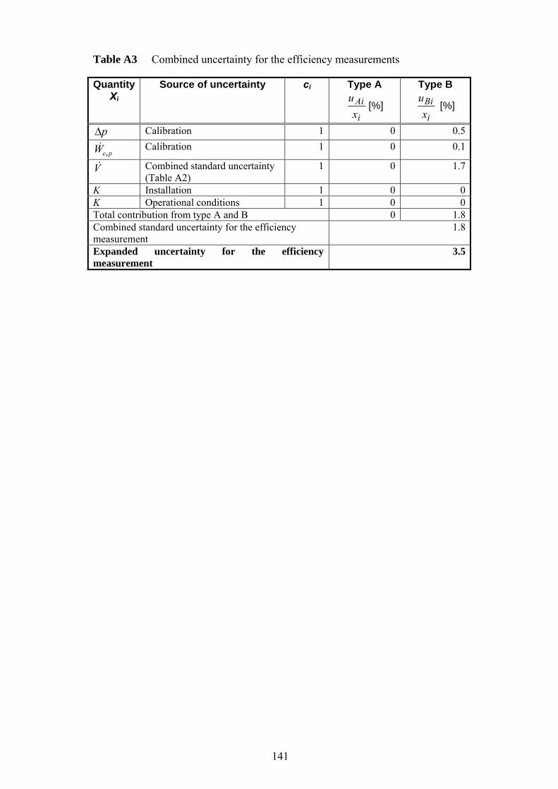
141

Table A3 Combined uncertainty for the efficiency measurements

Quantity Xi

Source of uncertainty ci Type A

i

Ai

x

u[%]

Type B

i

Bi

x

u [%]

Calibration 1 0 0.5

peW , Calibration 1 0 0.1

V Combined standard uncertainty (Table A2)

1 0 1.7

K Installation 1 0 0K Operational conditions 1 0 0Total contribution from type A and B 0 1.8Combined standard uncertainty for the efficiency measurement

1.8

Expanded uncertainty for the efficiency measurement

3.5

p