PART 1 Foundation

Chapter 1. Atomic structure

The origin of the elements

Before there was chemistry there should have been elements. How did the elements origin in the universe? Elements are the introduction to chemistry. Clear ideas that have been accumulated about the origin of elements come from cosmology which is investigating the nature and history of the universe and bed rock of chemistry and physics.

In investigating the nature and history of the universe we can hardly do better than to begin by examining what it is made of. The universe we see and measure is composed of an orderly yet diverse system of elements, from hydrogen to uranium. How did these elements come into being; from what primordial stuff were they made? Research into the origin of the elements is going forward in many directions but none of these have been as fruitful as the study of the quantities and ratios of elements on the earth and in stars. Clues such as meteorites also give us insight in what the universe is made of because they have undergone so little change, but the one method of research that has provided us with the most invaluable data is optical spectroscopy. (the study of light and its "characteristic spectrum" at optical wavelengths) Upon careful observation, the light emitted by stars in the universe yields some very interesting conclusions about the atomic make-up of the universe.

Eight Steps in the History of the Earth 1. The Big Bang 2.Star Formation 3. Supernova Explosion 4. Solar Nebula Condenses 5. Sun & Planetary Rings Form 6. Earth Forms 7. Earth's Core Forms 8. Oceans & Atmosphere Forms

Eight Steps in the History of the Earth

1. The Big Bang 2.Star Formation

3. Supernova Explosion

4. Solar Nebula Condenses

5a. Sun Form

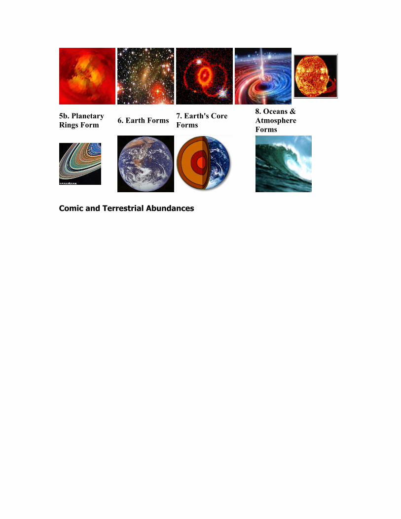
5b. Planetary Rings Form 6. Earth Forms 7. Earth's Core

Forms

8. Oceans & Atmosphere Forms

Comic and Terrestrial Abundances

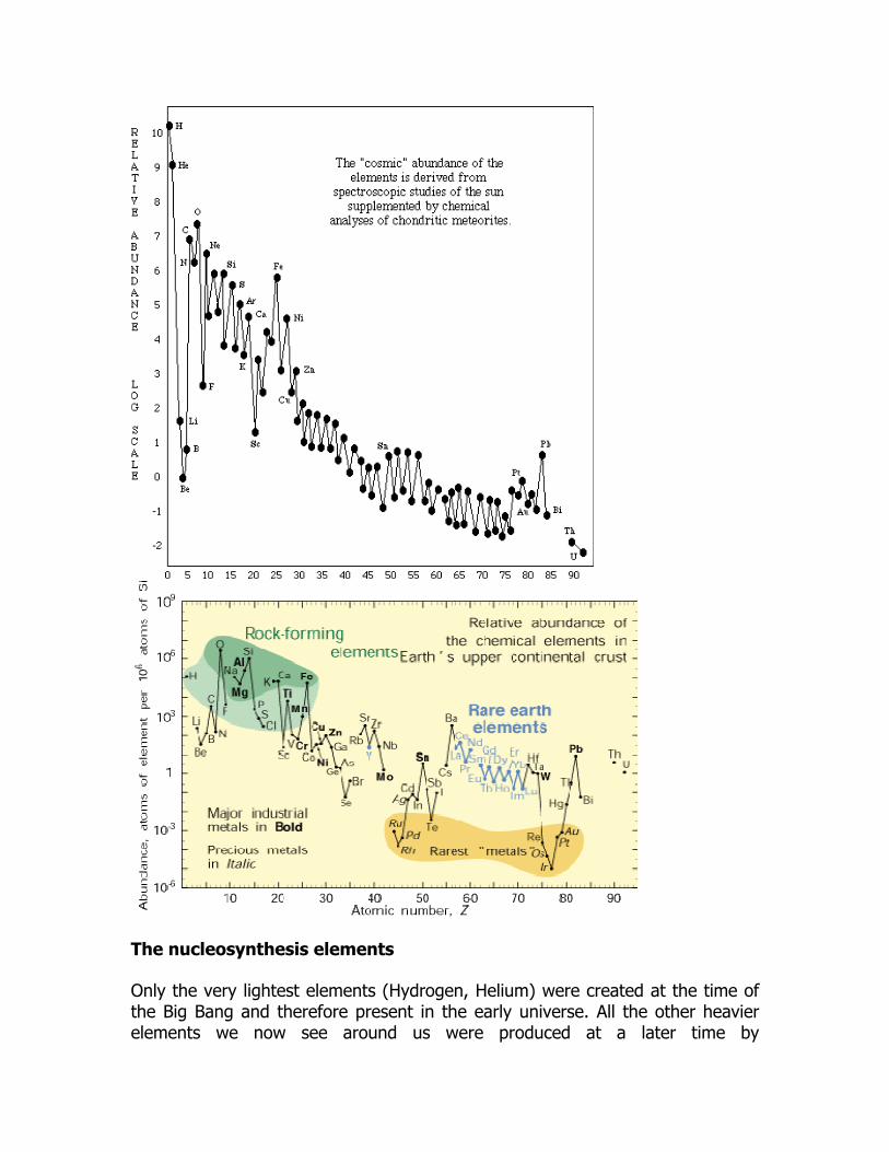
The nucleosynthesis elements

Only the very lightest elements (Hydrogen, Helium) were created at the time of the Big Bang and therefore present in the early universe. All the other heavier elements we now see around us were produced at a later time by

nucleosynthesis inside stars. In those"element factories", nuclei of the lighter elements are smashed together whereby they become the nuclei of heavier ones - this process is known as nuclear fusion. In our Sun and similar stars, Hydrogen is being fused into Helium. At some stage, Helium is fused into Carbon, then Oxygen, etc. The fusion process requires positively charged nuclei to move very close to each other before they can unite. But with increasing atomic mass and hence, increasing positive charge of the nuclei, the electric repulsion between the nuclei becomes stronger and stronger.

Nuclear Binding Energy

The binding energy of a nucleus is a measure of how tightly its protons and neutrons are held together by the nuclear forces. The binding energy per nucleon, the energy required to remove one neutron or proton from a nucleus, is a function of the mass number A. The curve of binding energy implies that if two light nuclei near the left end of the curve coalesce to form a heavier nucleus, or if a heavy nucleus at the far right splits into two lighter ones, more tightly bound nuclei result, and energy will be released. A nucleus always weighs less than the protons and neutrons that make it up. This lost mass is the nuclear binding energy: the energy that holds the nucleus together. (There are a lot of protons jammed in a very small space, which causes tremendous electrostatic repulsion. Large amounts of energy are needed to hold a nucleus together.) The binding energy can be computed from the mass-energy relationship ∆E = ∆mc2. The amount of missing mass is known as the mass defect.

Nuclear Binding Energy Curve for Elements expressed in MeV per nucleon.

To calculate the energy released, calculate the mass defect ( ), then multiply by 931.5 MeV/amu

Binding energy calculator

http://www.chem.latech.edu/~upali/chem281/calculators/Binding-Energy-Calculator.xls

Nuclear Reactions Light nuclides undergo fusion or bombardment to convert to other nuclides closer to the maximum value. Heavy nuclides undergo fission to give nuclides closer to the maximum value If a nuclear reaction gives products with a higher nuclear binding energy, then energy is released by the reaction.

Nuclear Fusion Reactions Nuclear energy, measured in millions of electron volts (MeV), is released by the fusion of two light nuclei, as when two heavy hydrogen nuclei, deuterons ( H), combine in the

reaction

producing a helium-3 atom, a free neutron ( n), and 3.2 MeV, or 5.1 × 10-13 J (1.2 × 10-13 cal). Nuclear Fission Reactions Nuclear energy is also released when the fission (breaking up of ) of a heavy nucleus such as 235U is induced by the absorption of a neutron as in

producing cesium-140, rubidium-93, three neutrons, and 200 MeV, or 3.2 × 10-11 J (7.7 × 10-12 cal). A nuclear fission reaction releases 10 million times as much energy as is released in a typical chemical reaction. The two key characteristics of nuclear fission important for the practical release of nuclear energy are both evident in equation (2). First, the energy per fission is very large. In practical units, the fission of 1 kg (2.2 lb) of uranium-235 releases 18.7 million kilowatt-hours as heat. Second, the fission process initiated by the absorption of one neutron in uranium-235 releases about 2.5 neutrons, on the average, from the split nuclei. The neutrons released in this manner quickly cause the fission of two more atoms, thereby releasing four or more additional neutrons and initiating a self-sustaining series of nuclear fissions, or a chain reaction, which results in continuous release of nuclear energy.

The nucleosynthesis of light elements

In the first few minutes after the Big Bang,

at temperatures

exceeding 109 K, several of the lightest elements and their isotopes were created. Most of the helium (He), essentially all of the deuterium (2H, the heavy isotope of hydrogen) and some lithium were thus

produced. Lithium has two stable isotopes, 7Li and 6Li, but the relevant

nuclear processes are such that the Big Bang

produced significant

amounts of only the

heavier one. Beryllium has one stable isotope (9Be), while boron has two (10B and 11B). These light elements were not produced in significant quantities in the Big Bang. Likewise, because of the rapid expansion of the universe and the concomitant decrease of the density and temperature, neither were the heavier elements (C, O , etc.).

The nucleosynthesis of heavy elements

Neutrons Capture reactions

The two principal paths to building "trans-Fe" elements are the s-process and the r-process. 1.S(slow)-process is the Slow addition of neutrons to nuclei with the neutron subsequently undergoing a β-decay (ejection of an e-) to change into a p+. This way atoms can slowly slowly walk their way up the Periodic table. It is much easier to add the changeless neutron to a nucleus than it is a p+.

56Fe26 + 3n0 -> 59Fe26

59Fe26 -> 59Co27 + e-1 + n0;

This works up to around Bismuth at atomic #83 and is though to occur in SNI and also in AGB stars during the thermal pulse stage. There is some direct evidence for the S-process occurring in some AGB stars. Technetium with atomic #43 is an S-process element that has a radioactive half-life of ~200,000 years. It has been detected in AGB stars that are MUCH older than that! The only thing that could be going on is the production of Tc in the star and then mixing of this to the surface via convection.

2.R(rapid)-process is the Rapid addition of neutrons to existing nuclei. The idea is that you add a bunch of neutrons which then start to decay into protons via β-decay in the nucleus. This increases the atomic number and is the way to produce the really heavy stuff. The R-process occurs only (we think) in SN and mostly in SNII. The evidence for R-process occuring is less direct. First, we see elements like Gold which are thought to only be produced via the R-process. It is also true that if we look at the oldest stars in the Galaxy, which were formed after only one or two SNII (these come from massive stars that have very short lives) had enriched the interstellar medium, the abundance of Iron is very low, but the abundaces of R-process elements are only moderately low.

The classification of the elements

Periodic Table History In the early 1800's Dobereiner noted that similar elements often had relative atomic masses, and DeChancourtois made a cylindrical table of elements to display the periodic reoccurrence of properties. Cannizaro determined atomic weights for the 60 or so elements known in the 1860s, then a table was arranged by Newlands, with the elements given a serial number in order of their atomic weights, beginning with Hydrogen. This

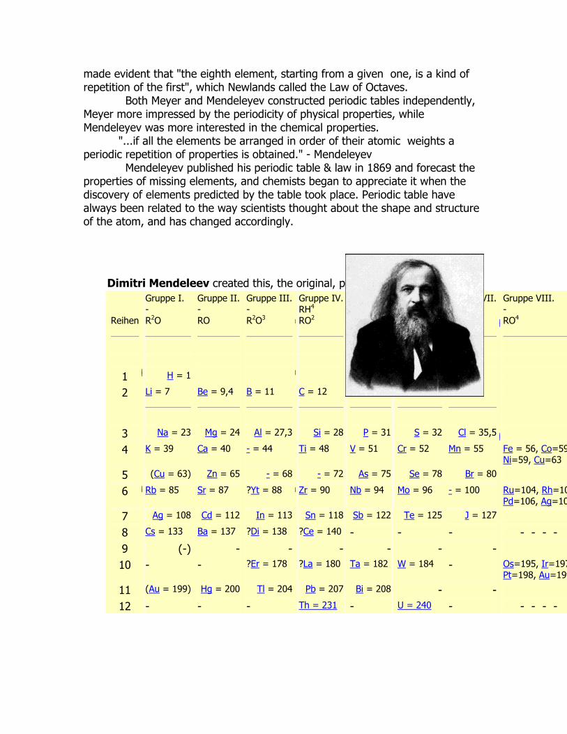
made evident that "the eighth element, starting from a given one, is a kind of repetition of the first", which Newlands called the Law of Octaves. Both Meyer and Mendeleyev constructed periodic tables independently, Meyer more impressed by the periodicity of physical properties, while Mendeleyev was more interested in the chemical properties. "...if all the elements be arranged in order of their atomic weights a periodic repetition of properties is obtained." - Mendeleyev Mendeleyev published his periodic table & law in 1869 and forecast the properties of missing elements, and chemists began to appreciate it when the discovery of elements predicted by the table took place. Periodic table have always been related to the way scientists thought about the shape and structure of the atom, and has changed accordingly.

Dimitri Mendeleev created this, the original, periodic table.

Reihen

Gruppe I. - R2O

Gruppe II.- RO

Gruppe III.- R2O3

Gruppe IV.RH4 RO2

Gruppe V.RH3 R2O5

Gruppe VI. RH2 RO3

Gruppe VII.RH R2O7

Gruppe VIII. - RO4

1 H = 1 2 Li = 7

Be = 9,4

B = 11

C = 12

N = 14

O = 16

F = 19

3 Na = 23 Mg = 24 Al = 27,3 Si = 28 P = 31 S = 32 Cl = 35,5

4 K = 39 Ca = 40 - = 44 Ti = 48 V = 51 Cr = 52 Mn = 55 Fe = 56, Co=59Ni=59, Cu=63

5 (Cu = 63) Zn = 65 - = 68 - = 72 As = 75 Se = 78 Br = 80

6 Rb = 85 Sr = 87 ?Yt = 88 Zr = 90 Nb = 94 Mo = 96 - = 100 Ru=104, Rh=10Pd=106, Ag=10

7 Ag = 108 Cd = 112 In = 113 Sn = 118 Sb = 122 Te = 125 J = 127

8 Cs = 133 Ba = 137 ?Di = 138 ?Ce = 140 - - - - - - - 9 (-) - - - - - -10 - - ?Er = 178 ?La = 180 Ta = 182 W = 184 - Os=195, Ir=197

Pt=198, Au=199

11 (Au = 199) Hg = 200 Tl = 204 Pb = 207 Bi = 208 - -

12

-

- - Th = 231 - U = 240

- - - - -

Dimitri Mendeleev

Organization of the Modern Periodic Table The `modern' periodic table is very much like a later table by Meyer, arranged, as was Mendeleyev's, according to the size of the atomic weight, but with Group 0 added by Ramsay. Later, the table was reordered by Mosely according to atomic numbers (nuclear charge) rather than by weight. The Periodic Law revealed important analogies among the 94 naturally occurring elements, and stimulated renewed interest in Inorganic Chemistry in the nineteenth century which has carried into the present with the creation of artificially produced, short lived elements of `atom smashers' and supercolliders of high energy physics. Harry D. Hubbard, of the United States National Bureau of Standards, modernized Mendeleyev's periodic table, and his first work was published in 1924. This was known as the "Periodic Chart of the Atoms". Into the 1930s the heaviest elements were being put up in the body of the periodic table, and Dr.Glenn T.Seaborg in 1968 "plucked those out" while working with Fermi in Chicago, naming them the Actinide series, which later permitted proper placement of subsequently 'created' elements - the Transactinides, changing the periodic table yet again. These elements were shown separate from the main body of the table.

The Alexander Arrangement of the Elements, a three-dimensional periodic chart designed and patented by Roy Alexander and introduced in 1994, retains the separate Lanthanide and Actinide series, but integrates them at the same time, made possible by using all three dimensions Further improvement provided by the Alexander Arrangement of the Elements is location of all the element data blocks in a continuous sequence according to atomic numbers while retaining all accepted property interrelationships. This eases use & understanding of the immense correlative power of the periodic chart in teaching, learning, and working with chemistry. Periodic table is an arrangement of all known element according to their atomic number and chemical properties. This table contains vertical columns called groups and horizontal columns called periods. All elements in a group have similar chemical properties. These groups are number from 1 - 8, left to right and some of groups have their own names.

group I - alkali metal: Li, Na, K Rb, Cs, Fr group II - alkaline earth metals: Be, Mg, Ca, Sr, Ba, Ra

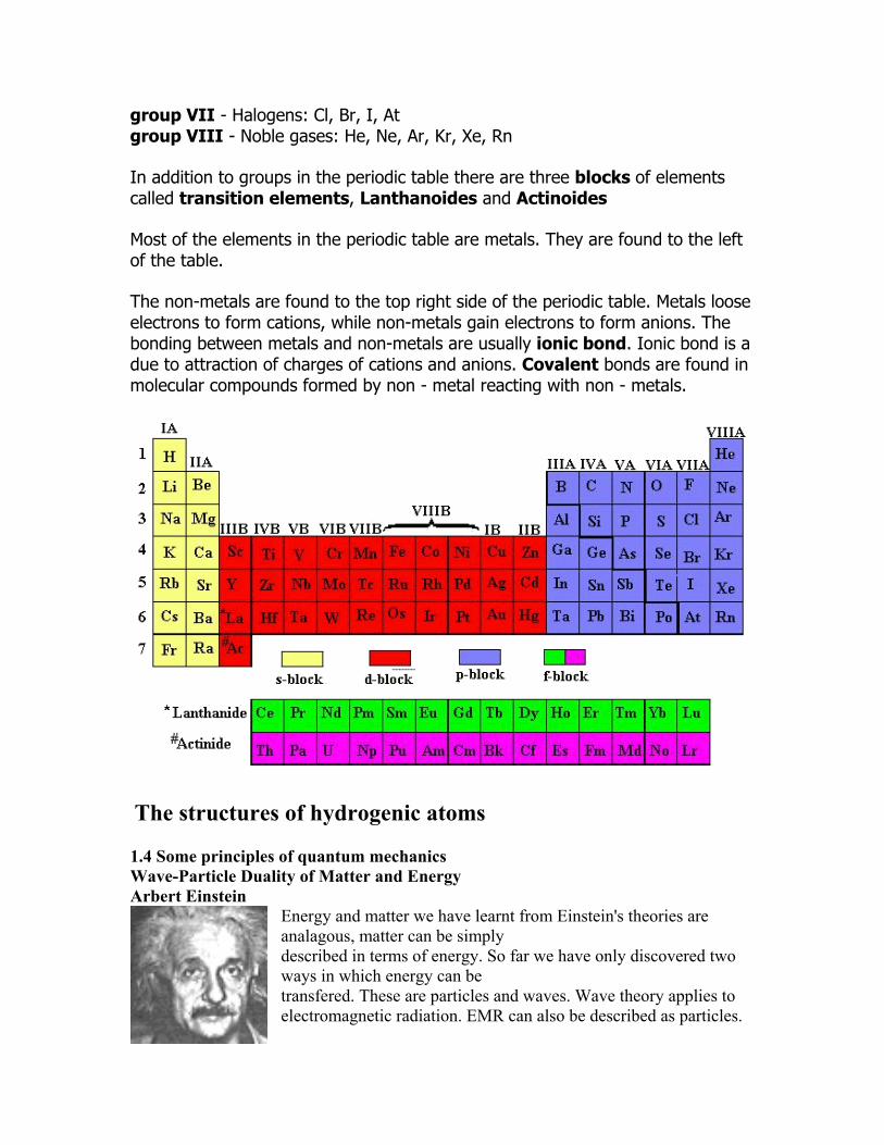
group VII - Halogens: Cl, Br, I, At group VIII - Noble gases: He, Ne, Ar, Kr, Xe, Rn

In addition to groups in the periodic table there are three blocks of elements called transition elements, Lanthanoides and Actinoides

Most of the elements in the periodic table are metals. They are found to the left of the table.

The non-metals are found to the top right side of the periodic table. Metals loose electrons to form cations, while non-metals gain electrons to form anions. The bonding between metals and non-metals are usually ionic bond. Ionic bond is a due to attraction of charges of cations and anions. Covalent bonds are found in molecular compounds formed by non - metal reacting with non - metals.

The structures of hydrogenic atoms

1.4 Some principles of quantum mechanics Wave-Particle Duality of Matter and Energy Arbert Einstein

Energy and matter we have learnt from Einstein's theories are analagous, matter can be simply described in terms of energy. So far we have only discovered two ways in which energy can be transfered. These are particles and waves. Wave theory applies to electromagnetic radiation. EMR can also be described as particles.

quanta :A particles of light energy. Quantum: One particle of light with a certain energy. Photon: A stream of Quanta Wave theory could be applied to electrons. What is a wave-mechanical model? motions of a vibrating string shows one dimensional motion. Energy of the vibrating string is quantized Energy of the waves increased with the nodes. Nodes are places were string is stationary. Number of nodes gives the quantum number. One dimensional motion gives one quantum number.

Wave properties of Electron The electron is clearly a particle as the experiments of J J Thomson show. He calculated that there was a clear e/m ratio and that the charge on any electron is 1.6E-19 Coulombs. However, experiments by Davisson and Germer show that electrons can display diffraction, an obvious wave property. The first complete evidence of deBroglie's hyprothesis came from two physicists working at the Bell Laboratories in the USA in 1926. Using beams as Thomson did in electron diffraction they scattered electrons off Nickel crystals and analysed how the electrons were more likely to appear at certain angles than others. De Broglie suggested that electrons have wave properties to account for why their energy was quantized. He reasoned that the electron in the hydrogen atom was fixed in the space around the nucleus. He felt that the electron would best be represented as a standing wave. As a standing wave, each electron’s path must equal a whole number times the wavelength.

Electrons as de Broglie waves De Broglie proposed that all particles have a wavelength as related by:

λ = h/mv

l = wavelength, meters h = Plank’s constant m = mass, kg v = frequency, m/s

An unstable wave orbit

Returning now to the problem of the atom, it was realized that if, for the moment, we pictured the electron not as a particle but as a wave, then it was possible to get stable configurations. Imagine trying to establish a wave in a circular path about a nucleus. One possibility might be as below.

For this configuration, when one starts the wave at a given point, one ends up after one complete revolution at a different point on the wave. The incoming wave will then be out of phase with the original wave, and destructive interference will occur. However, certain stable configurations are possible, as is illustrated below.

In this case, the wave ends up in phase with the original wave after one complete revolution, and constructive interference results. Such a pattern would result in a stable orbit. This type of wave is called a standing wave, and are common in other contexts; for example, they can be established on a string attached to a wall if the string is moved up and down at exactly the right speed (such a wave would appear not to be moving, which is why it's called a standing wave). The Heisenberg Uncertainty Principle There is a theoretical limit on the exactness with which a particle can be pinned-down (usually in terms of its position and momentum): ∆x.∆p > h/2π where ∆x is the uncertainty in position and ∆p the uncertainty in momentum.

The Schrödinger Wave Equation and Its Significance The Schrödinger Wave Equation In its most general form the equation looks like this:

HΨ = EΨ

Ψ is a function describing the electron in terms of wave properties, such that it can be used to calculate the amplitude of the wave at some point in space. This property does not have much physical meaning, but by integrating Ψ2 over a volume of space, we can

A stable wave orbit

determine the probability of finding the electron within that space.

H is called the Hamiltonian operator and represents a series of mathematical operations that must be performed on Ψ which will give back Ψ multiplied by an energy E for the electron. Only Ψ functions for which this is true are "proper" wave-functions, called "eigenfuctions" and the E's that go with them are called "eigenvalues". ("Eigen" is German for "unique".)

H is defined for the system being described, for example one nucleus and one electron (hydrogen) or two nuclei and one electron (H2

+), so the trick is to find the eigenfunctions which work. Let's see how this works in a model system - not an electron, but a vibrating string: The Vibrating String and the "Particle in a One-dimensional Box"

The following diagrams illustrate vibrations on stretched strings. The two curves indicate the extremes of the motion, and the formulae apply to the red one.

ψ = sin(1πx/l)

ψ = sin(2πx/l)

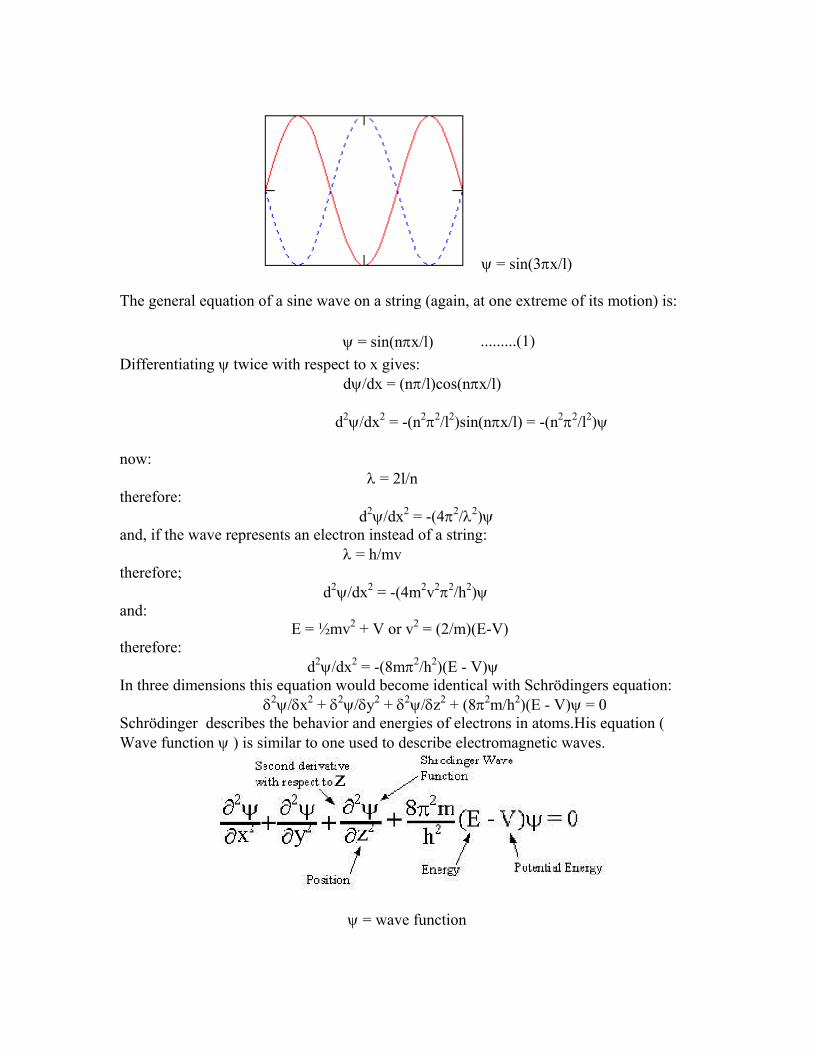
ψ = sin(3πx/l)

The general equation of a sine wave on a string (again, at one extreme of its motion) is:

ψ = sin(nπx/l) .........(1)Differentiating ψ twice with respect to x gives: dψ/dx = (nπ/l)cos(nπx/l)

d2ψ/dx2 = -(n2π2/l2)sin(nπx/l) = -(n2π2/l2)ψ

now: λ = 2l/n therefore: d2ψ/dx2 = -(4π2/λ2)ψ and, if the wave represents an electron instead of a string: λ = h/mv therefore; d2ψ/dx2 = -(4m2v2π2/h2)ψ and: E = ½mv2 + V or v2 = (2/m)(E-V) therefore: d2ψ/dx2 = -(8mπ2/h2)(E - V)ψ In three dimensions this equation would become identical with Schrödingers equation: δ2ψ/δx2 + δ2ψ/δy2 + δ2ψ/δz2 + (8π2m/h2)(E - V)ψ = 0 Schrödinger describes the behavior and energies of electrons in atoms.His equation ( Wave function ψ ) is similar to one used to describe electromagnetic waves.

ψ = wave function

E = total energy V = potential energy

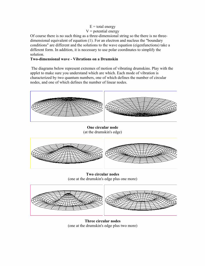
Of course there is no such thing as a three-dimensional string so the there is no three-dimensional equivalent of equation (1). For an electron and nucleus the "boundary conditions" are different and the solutions to the wave equation (eigenfunctions) take a different form. In addition, it is necessary to use polar coordinates to simplify the solution. Two-dimensional wave - Vibrations on a Drumskin

The diagrams below represent extremes of motion of vibrating drumskins. Play with the applet to make sure you understand which are which. Each mode of vibration is characterized by two quantum numbers, one of which defines the number of circular nodes, and one of which defines the number of linear nodes.

One circular node (at the drumskin's edge)

Two circular nodes (one at the drumskin's edge plus one more)

Three circular nodes (one at the drumskin's edge plus two more)

One transverse node (plus a circular one at the drumskin's edge)

Two transverse nodes (plus one at the drumskin's edge)

Two transverse nodes plus two circular nodes

These vibrations are much easier to visualize when animated. Separation of the Eigenfunctions into Radial and Angular Components It turns out to be much easier to solve the three-dimensional Schrödinger equation if it is transformed to polar coordinates:

Once this is done, the Ψ is replaced by: Ψ(r,θ,φ) = R(r).Θ(θ).Φ(φ)

R(r) the radial wave function. The solutions (eigenfunctions) R(r) are called the radial wave functions. (Θ(θ).Φ(φ)) angular function The product of the other two (Θ(θ).Φ(φ)) are the angular functions. Some radial functions are depicted graphically below. Note that the three quantum numbers (n, l and ml) which are generated as part of the process of solving the equations are built into the resulting functions so you do not see them in the formulae explicitly. Note the sign changes due to the polynomial part of the equation, and also, the overall exponential decay with increasing r: Ψ2 and the electron "density" The quantity Ψ has no physical meaning, but Ψ2 integrated over a chosen volume represents the probability of finding the electron within that volume. The alternative way of interpreting Ψ2 is as the electron "density" of a distributed electron "cloud". The other function depicted in the graphs is 4πr2R2(r). This function, integrated over a small range of r (dr) gives the probability of finding the electron in a spherical shell of thickness dr. It allows the calculation of the most probable distance from the nucleus for the electron. These distances correspond exactly to the Bohr theory radii. This is most evident for the lowest energy solution (1s). Mathematical expression of hydrogen like orbitals in polar coordinates: ψn, l, ml, ms (r, θ, φ) = R n, l (r) Y l, ml (θ, φ) R n, l (r ) = Radial Wave Function Y l, ml (θ, φ) =Angular Wave Function Plots of radial probability function: [R n, l (r )]2 Vs r (radius) for various n and l values Radial probability function electron in 1s orbital

Radial probability function electron in 2s orbital

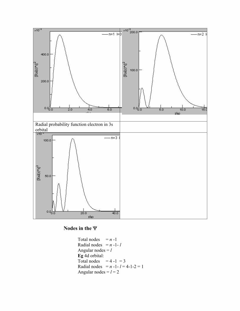
Radial probability function electron in 3s orbital

Nodes in the Ψ

Total nodes = n -1 Radial nodes = n -1- l Angular nodes = l Eg 4d orbital: Total nodes = 4 -1 = 3 Radial nodes = n -1- l = 4-1-2 = 1 Angular nodes = l = 2

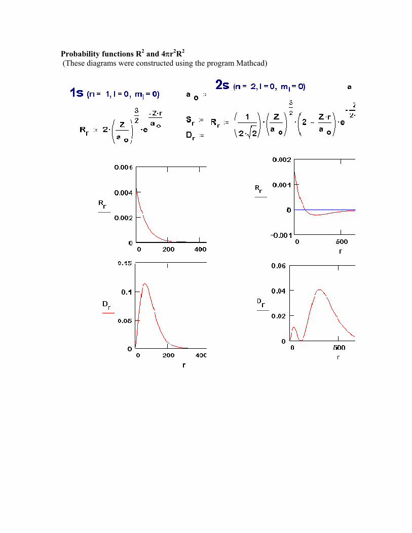
Probability functions R2 and 4πr2R2 (These diagrams were constructed using the program Mathcad)

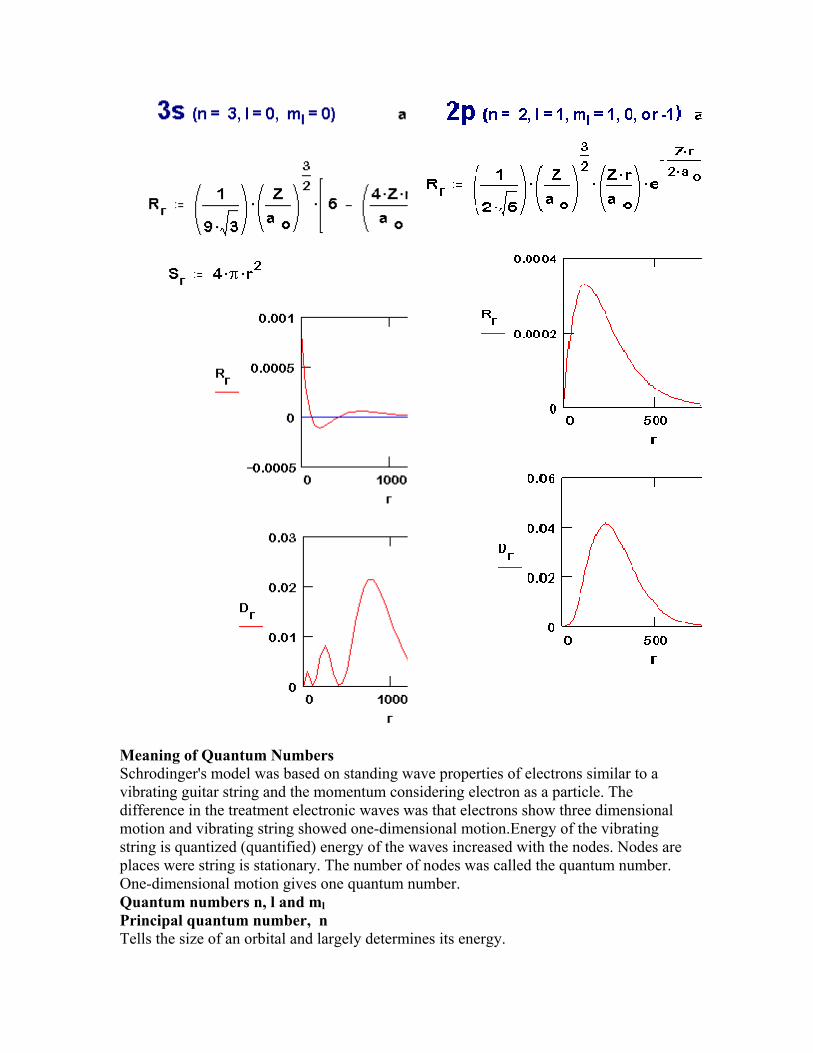
Meaning of Quantum Numbers Schrodinger's model was based on standing wave properties of electrons similar to a vibrating guitar string and the momentum considering electron as a particle. The difference in the treatment electronic waves was that electrons show three dimensional motion and vibrating string showed one-dimensional motion.Energy of the vibrating string is quantized (quantified) energy of the waves increased with the nodes. Nodes are places were string is stationary. The number of nodes was called the quantum number. One-dimensional motion gives one quantum number. Quantum numbers n, l and ml Principal quantum number, n Tells the size of an orbital and largely determines its energy.

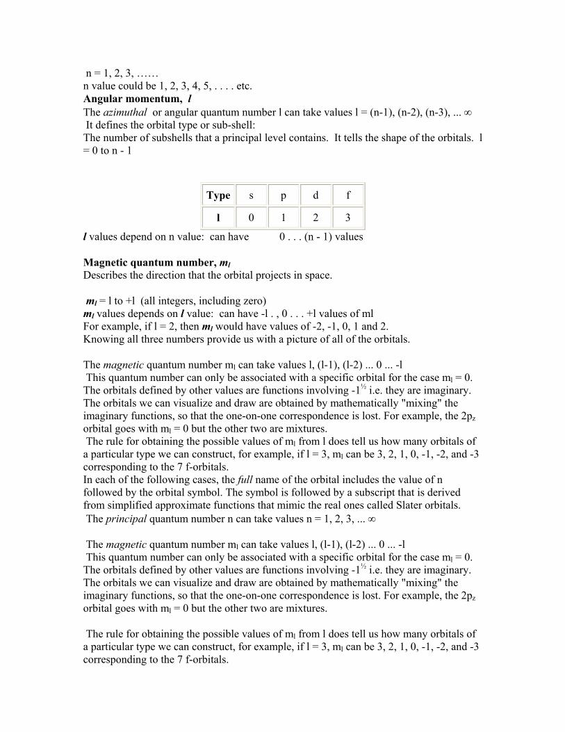
n = 1, 2, 3, …… n value could be 1, 2, 3, 4, 5, . . . . etc. Angular momentum, l The azimuthal or angular quantum number l can take values l = (n-1), (n-2), (n-3), ... ∞ It defines the orbital type or sub-shell: The number of subshells that a principal level contains. It tells the shape of the orbitals. l = 0 to n - 1

Type s p d f

l 0 1 2 3

l values depend on n value: can have 0 . . . (n - 1) values

Magnetic quantum number, ml Describes the direction that the orbital projects in space.

ml = l to +l (all integers, including zero) ml values depends on l value: can have -l . , 0 . . . +l values of ml For example, if l = 2, then ml would have values of -2, -1, 0, 1 and 2. Knowing all three numbers provide us with a picture of all of the orbitals.

The magnetic quantum number ml can take values l, (l-1), (l-2) ... 0 ... -l This quantum number can only be associated with a specific orbital for the case ml = 0. The orbitals defined by other values are functions involving -1½ i.e. they are imaginary. The orbitals we can visualize and draw are obtained by mathematically "mixing" the imaginary functions, so that the one-on-one correspondence is lost. For example, the 2pz orbital goes with ml = 0 but the other two are mixtures. The rule for obtaining the possible values of ml from l does tell us how many orbitals of a particular type we can construct, for example, if l = 3, ml can be 3, 2, 1, 0, -1, -2, and -3 corresponding to the 7 f-orbitals. In each of the following cases, the full name of the orbital includes the value of n followed by the orbital symbol. The symbol is followed by a subscript that is derived from simplified approximate functions that mimic the real ones called Slater orbitals. The principal quantum number n can take values n = 1, 2, 3, ... ∞

The magnetic quantum number ml can take values l, (l-1), (l-2) ... 0 ... -l This quantum number can only be associated with a specific orbital for the case ml = 0. The orbitals defined by other values are functions involving -1½ i.e. they are imaginary. The orbitals we can visualize and draw are obtained by mathematically "mixing" the imaginary functions, so that the one-on-one correspondence is lost. For example, the 2pz orbital goes with ml = 0 but the other two are mixtures.

The rule for obtaining the possible values of ml from l does tell us how many orbitals of a particular type we can construct, for example, if l = 3, ml can be 3, 2, 1, 0, -1, -2, and -3 corresponding to the 7 f-orbitals.

In each of the following cases, the full name of the orbital includes the value of n followed by the orbital symbol. The symbol is followed by a subscript that is derived from simplified approximate functions that mimic the real ones called Slater orbitals. Spin Quantum Number ms should always be -1/2 or +1/2 For the electron 3 Quantum numbers for motion in 3 dimension (x, y, z directions in space) are necessary. Fourth Quantum number was necessary due to spin motion of the electron. According to wave-mechanical model an electron has four Quantum numbers (Q.N.): n = Principle Q.N.; l =Angular Momentum Q.N.; ml = Magnetic Q.N.; ms = Spin Q.N. Schrödinger introduced the notion of treating electrons as standing waves - a novel move away from thinking of electrons as particles.

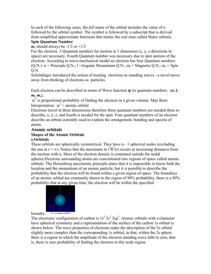
Each electron can be described in terms of Wave function ψ its quantum numbers. (n, l, ml, ms), ψ2 is proportional probablity of finding the electron in a given volume. Max Born Interpretation: ψ2 = atomic orbital Electrons travel in three dimensions therefore three quantum numbers are needed three to describe, x, y, z, and fourth is needed for the spin. Four quantum numbers of an electron describe an orbital currently used to explain the arrangement, bonding and spectra of atoms. Atomic orbitals Shapes of the Atomic Orbitals s-Orbitals These orbitals are spherically symmetrical. They have n - 1 spherical nodes (excluding the one at r = ∞). Notice that the maximum in r2R2(r) occurs at increasing distances from the nucleus with n. Most of the electron density is contained outside the nodal spheres.Electrons surrounding atoms are concentrated into regions of space called atomic orbitals. The Heisenberg uncertainty principle states that it is impossible to know both the location and the momentum of an atomic particle, but it is possible to describe the probability that the electron will be found within a given region of space. The boundries of an atomic orbital are commonly drawn to the region of 90% probability; there is a 90% probability that at any given time, the electron will be within the specified

boundry. The electronic configuration of carbon is 1s2 2s2 2sp3. Atomic orbitals with s-character have spherical symmetry and a representation of the surface of the carbon 1s orbital is shown below. The wave properties of electrons make the description of the 2s orbital slightly more complex than the corresponding 1s orbital, in that, within the 2s sphere there is a region in which the amplitude of the electron standing wave falls to zero, that is, there is zero probability of finding the electron in this node region.

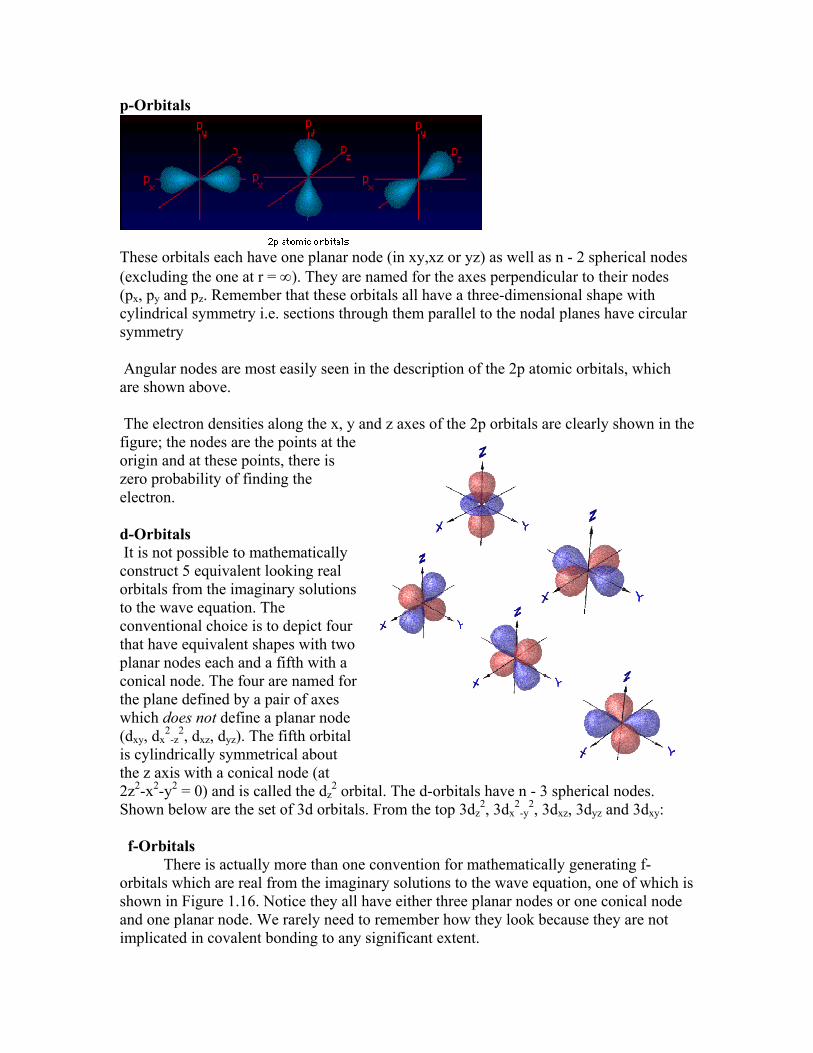
p-Orbitals

These orbitals each have one planar node (in xy,xz or yz) as well as n - 2 spherical nodes (excluding the one at r = ∞). They are named for the axes perpendicular to their nodes (px, py and pz. Remember that these orbitals all have a three-dimensional shape with cylindrical symmetry i.e. sections through them parallel to the nodal planes have circular symmetry

Angular nodes are most easily seen in the description of the 2p atomic orbitals, which are shown above. The electron densities along the x, y and z axes of the 2p orbitals are clearly shown in the figure; the nodes are the points at the origin and at these points, there is zero probability of finding the electron.

d-Orbitals It is not possible to mathematically construct 5 equivalent looking real orbitals from the imaginary solutions to the wave equation. The conventional choice is to depict four that have equivalent shapes with two planar nodes each and a fifth with a conical node. The four are named for the plane defined by a pair of axes which does not define a planar node (dxy, dx

2-z

2, dxz, dyz). The fifth orbital is cylindrically symmetrical about the z axis with a conical node (at 2z2-x2-y2 = 0) and is called the dz

2 orbital. The d-orbitals have n - 3 spherical nodes. Shown below are the set of 3d orbitals. From the top 3dz

2, 3dx2

-y2, 3dxz, 3dyz and 3dxy:

f-Orbitals There is actually more than one convention for mathematically generating f-orbitals which are real from the imaginary solutions to the wave equation, one of which is shown in Figure 1.16. Notice they all have either three planar nodes or one conical node and one planar node. We rarely need to remember how they look because they are not implicated in covalent bonding to any significant extent.

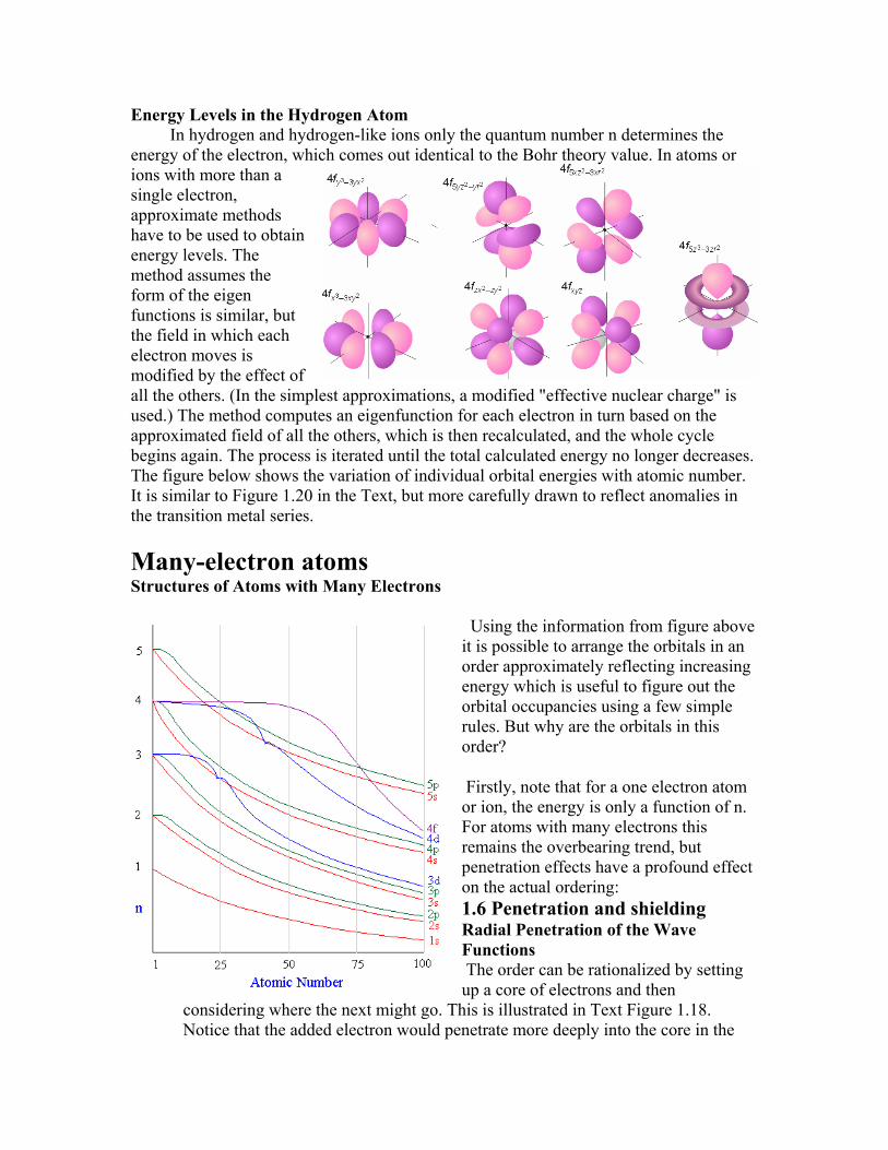
Energy Levels in the Hydrogen Atom In hydrogen and hydrogen-like ions only the quantum number n determines the energy of the electron, which comes out identical to the Bohr theory value. In atoms or ions with more than a single electron, approximate methods have to be used to obtain energy levels. The method assumes the form of the eigen functions is similar, but the field in which each electron moves is modified by the effect of all the others. (In the simplest approximations, a modified "effective nuclear charge" is used.) The method computes an eigenfunction for each electron in turn based on the approximated field of all the others, which is then recalculated, and the whole cycle begins again. The process is iterated until the total calculated energy no longer decreases. The figure below shows the variation of individual orbital energies with atomic number. It is similar to Figure 1.20 in the Text, but more carefully drawn to reflect anomalies in the transition metal series.

Many-electron atoms Structures of Atoms with Many Electrons

Using the information from figure above it is possible to arrange the orbitals in an order approximately reflecting increasing energy which is useful to figure out the orbital occupancies using a few simple rules. But why are the orbitals in this order?

Firstly, note that for a one electron atom or ion, the energy is only a function of n. For atoms with many electrons this remains the overbearing trend, but penetration effects have a profound effect on the actual ordering: 1.6 Penetration and shielding Radial Penetration of the Wave Functions The order can be rationalized by setting up a core of electrons and then

considering where the next might go. This is illustrated in Text Figure 1.18. Notice that the added electron would penetrate more deeply into the core in the

orbital with the lowest l (s more than p more than d). Do not be mislead by the position of the main maximum in each curve: it is the little "bumps" towards the nucleus that make the difference. Since the stabilization of the electron is directly related to the nuclear charge it "feels" (the effective nuclear charge), the greater the penetration, the better. Effective Nuclear charge (Zeff): Nuclear charge felt by electrons. Zeff is less than atomic number (Z) since in polyelectronic atoms electrons screen each other from the nucleus. Many atomic properties are directly related to the magnitude of Zeff. Variation of Zeff has been used to explain atomic property trends going across a period or down a group in the periodic table.

Zeff increase going across a period

Zeff decrease going down a group

Slater's Rules for Effective Nuclear Charge This set of simple rules for approximating the effective nuclear charge was proposed a number of years ago by Professor John C. Slater, a former faculty member at M.I.T. Derive the Zeff for the elements Li through Ne and compare your results with the experimental ionization energies and atomic radii for these elements. Are your calculations consistent with the experimental values for ionization and with the radii? Calculate Zeff for the group IA elements. What do you find? How do you rationalize your results with the experimental ionization energies of these elements? Slater's Rules for Estimating Z*

Z* = Z - σ Group the orbitals acccording to the following pattern (which differs from the filling order) and write out the configuration:

{(1s)}{(2s,2p)}{(3s,3p) (3d)}{(4s,4p) (4d) (4f)}{(5s,5p) etc... Now consider one electron and the influence of the Z-1 others on it: If the electron is an s or p electron:

If the electron is one of two 1s electrons, the shielding constant σ is 0.30 - stop here, otherwise: All the other electrons in groups to the right of the electron in question have zero contribution to σ. Each electron in the same (ns,np) group has contribution 0.35 to σ. Each electron in the n-1 shell contributes 0.85. All those electrons in shells n-2 or lower contribute 1.0 to σ. If the electron is in a d or f-orbital:

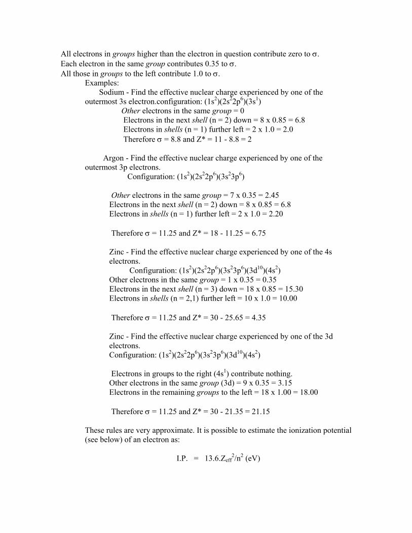
All electrons in groups higher than the electron in question contribute zero to σ. Each electron in the same group contributes 0.35 to σ. All those in groups to the left contribute 1.0 to σ.

Examples: Sodium - Find the effective nuclear charge experienced by one of the outermost 3s electron.configuration: (1s2)(2s22p6)(3s1) Other electrons in the same group = 0 Electrons in the next shell (n = 2) down = 8 x 0.85 = 6.8 Electrons in shells (n = 1) further left = 2 x 1.0 = 2.0 Therefore σ = 8.8 and Z* = 11 - 8.8 = 2

Argon - Find the effective nuclear charge experienced by one of the outermost 3p electrons. Configuration: (1s2)(2s22p6)(3s23p6)

Other electrons in the same group = 7 x 0.35 = 2.45 Electrons in the next shell (n = 2) down = 8 x 0.85 = 6.8 Electrons in shells (n = 1) further left = 2 x 1.0 = 2.20

Therefore σ = 11.25 and Z* = 18 - 11.25 = 6.75

Zinc - Find the effective nuclear charge experienced by one of the 4s electrons. Configuration: (1s2)(2s22p6)(3s23p6)(3d10)(4s2) Other electrons in the same group = 1 x 0.35 = 0.35 Electrons in the next shell (n = 3) down = 18 x 0.85 = 15.30 Electrons in shells (n = 2,1) further left = 10 x 1.0 = 10.00

Therefore σ = 11.25 and Z* = 30 - 25.65 = 4.35

Zinc - Find the effective nuclear charge experienced by one of the 3d electrons. Configuration: (1s2)(2s22p6)(3s23p6)(3d10)(4s2)

Electrons in groups to the right (4s1) contribute nothing. Other electrons in the same group (3d) = 9 x 0.35 = 3.15 Electrons in the remaining groups to the left = 18 x 1.00 = 18.00

Therefore σ = 11.25 and Z* = 30 - 21.35 = 21.15

These rules are very approximate. It is possible to estimate the ionization potential (see below) of an electron as:

I.P. = 13.6.Zeff2/n2 (eV)

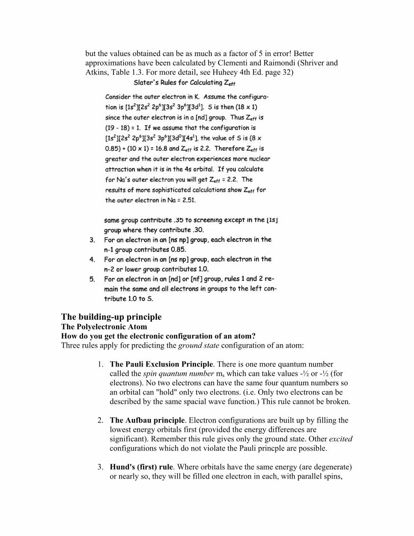
but the values obtained can be as much as a factor of 5 in error! Better approximations have been calculated by Clementi and Raimondi (Shriver and Atkins, Table 1.3. For more detail, see Huheey 4th Ed. page 32)

The building-up principle The Polyelectronic Atom How do you get the electronic configuration of an atom? Three rules apply for predicting the ground state configuration of an atom:

1. The Pauli Exclusion Principle. There is one more quantum number called the spin quantum number ms which can take values -½ or -½ (for electrons). No two electrons can have the same four quantum numbers so an orbital can "hold" only two electrons. (i.e. Only two electrons can be described by the same spacial wave function.) This rule cannot be broken.

2. The Aufbau principle. Electron configurations are built up by filling the lowest energy orbitals first (provided the energy differences are significant). Remember this rule gives only the ground state. Other excited configurations which do not violate the Pauli princple are possible.

3. Hund's (first) rule. Where orbitals have the same energy (are degenerate) or nearly so, they will be filled one electron in each, with parallel spins,

before pairing begins. Other configurations are excited states i.e. not forbidden.

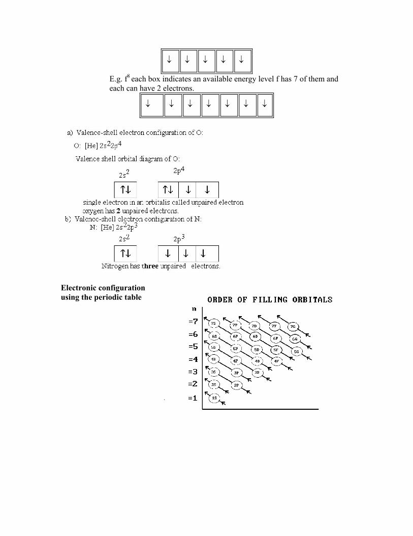
• Use periodic table • Periodic table is divided into orbital blocks • Each period:represents a shell or n • Start writing electron configuration • Using following order • 1s 2s 2p 3s 3p 4s 3d 4p 5s 4d 5p 6s 4f 5d 6p 7s 5f 6d… (building up (Auf

Bau) • principle:)

What is Building Up (Auf Bau) Principle? Scheme used by chemist to obtain electronic configuration of a multi-electron atom in the ground state by filling hydrogen like atomic orbital starting with lowest energy. 1s 2s 2p3s 3p 4s 3d 4p 5s 4d 5p 6s 4f 5d 6p 7s 5f 6d… (building up principle)

What is Pauli Exclusion Principle? If two or more orbitals exist at the same energy level, they are degenerate. Do not pair the electrons until you have to. Electrons in an atom cannot have all four of their quantum numbers equal. Eg. He: 1s2 electron orbital n l ml ms __________________________________ 1 1s1 1 0 0 1/2 ( ↓ ) 2 1s2 1 0 0 -1/2 ( )

Hund’s Rule Rule to fill electrons into p,d,f orbitals containing more than one sublevel of the same energy.

filling p, d, f orbitals: Put electrons into separate orbitals of the subshell with parallel spins before pairing electrons.Hund's rule: filling p, d, f orbitals.

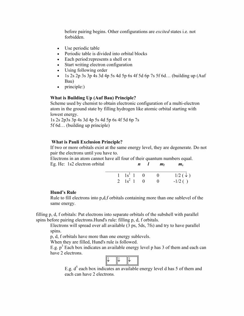
Electrons will spread over all available (3 ps, 5ds, 7fs) and try to have parallel spins. p, d, f orbitals have more than one energy sublevels. When they are filled, Hund's rule is followed. E.g. p3 Each box indicates an available energy level p has 3 of them and each can have 2 electrons.

↓ ↓ ↓

E.g. d5 each box indicates an available energy level d has 5 of them and each can have 2 electrons.

↓ ↓ ↓ ↓ ↓

E.g. f8 each box indicates an available energy level f has 7 of them and each can have 2 electrons.

↓ ↓ ↓ ↓ ↓ ↓ ↓

Electronic configuration using the periodic table

• To write the ground-state electron configuration of an element: • Starting with hydrogen, go through the elements in order of increasing atomic

number • As you move across a period • Add electrons to the ns orbital as you pass through groups IA (1) and IIA (2). • Add electrons to the np orbital as you pass through Groups IIIA (13) to 0 (18). • Add electrons to (n-1) d orbitals as you pass through IIIB (3) to IIB(12) and add

electrons to (n-2) f orbitals as you pass through the f -block.

Examples Regular format

O 1s2 2s2 2p4 Ti 1s2 2s2 2p6 3s2 3p6 3d2 4s2 Br 1s2 2s22p6 3s2 3p6 3d10 4s2 4p5 Core format O [He] 2s2 2p4 Ti [Ar] 3d2 4s2 Br [Ar] 3d10 4s2 4p5

Elements of Period One

Hydrogen to Helium

Z=1 to

1s1 to

No choice here! The 2s is significantly higher in energy. the second electron pairs (opposite spin)

Z=2 (K-shell)

with the other sharing the 1s wavefunction.

Elements of Period Two

Lithium Beryllium

Z=3 Z=4 (L-shell, part)

1s22s1 1s22s2

The effect of the greater penetration of the 2s orbital favours it over the 2p as the home for the next two electrons.

Boron to Neon

Z=5 to Z=10 (L-shell, then rest)

1s22s22p1 to 1s22s22p6

Add one electron to each 2p orbital, spins parallel, until each of the three has one electron, and then begin pairing. If it is necessary to be specific, use a diagram showing individual orbitals and electron spins as arrows. It does not matter which combination of orbitals are chosen when a choice exists, nor which spin is chosen, as long as they are parallel as far as possible.

Elements of Period Three

Sodium to Argon

Z=11 to Z=18 (M-shell)

[neon]3s1 to [Neon]3s23p6

These follow the pattern of the period from lithium to neon. The core, [neon] means the configuration of neon.

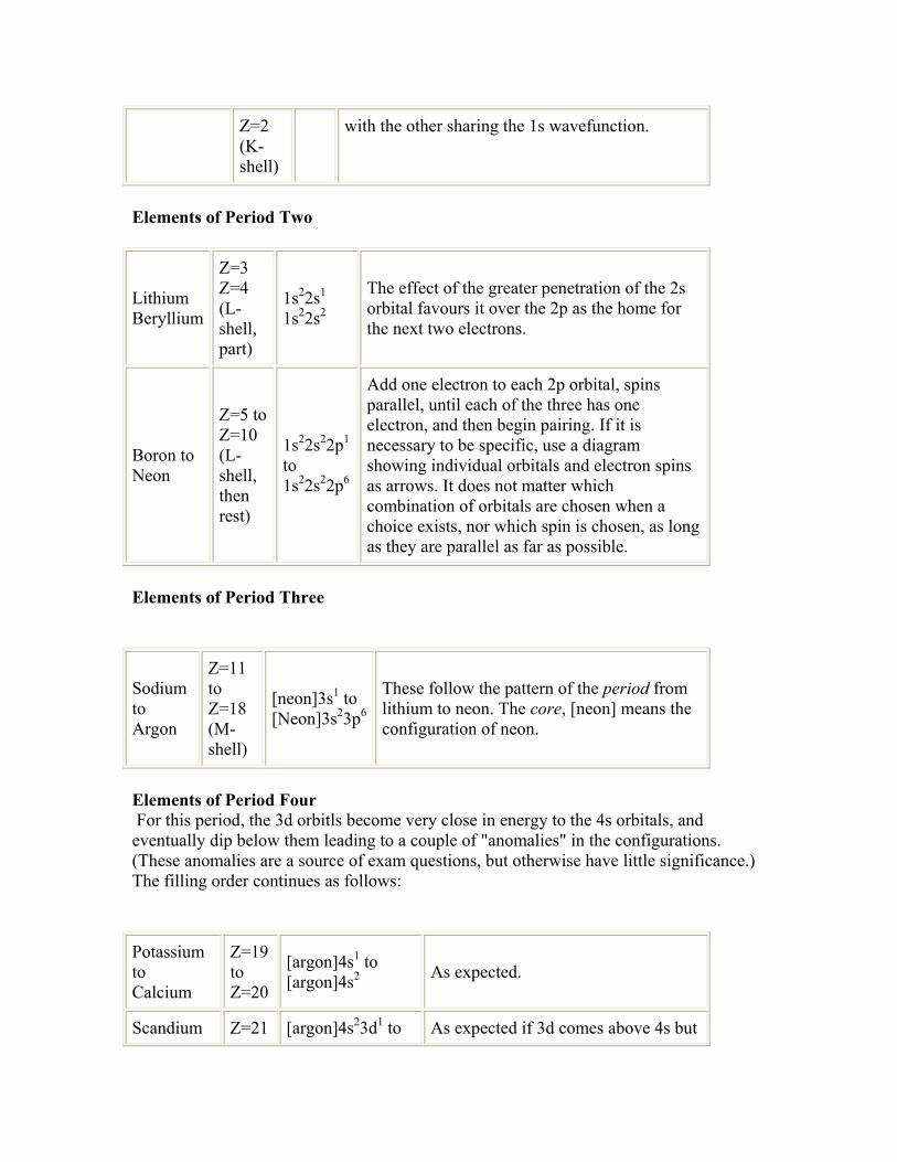
Elements of Period Four For this period, the 3d orbitls become very close in energy to the 4s orbitals, and eventually dip below them leading to a couple of "anomalies" in the configurations. (These anomalies are a source of exam questions, but otherwise have little significance.) The filling order continues as follows:

Potassium to Calcium

Z=19 to Z=20

[argon]4s1 to [argon]4s2 As expected.

Scandium Z=21 [argon]4s23d1 to As expected if 3d comes above 4s but

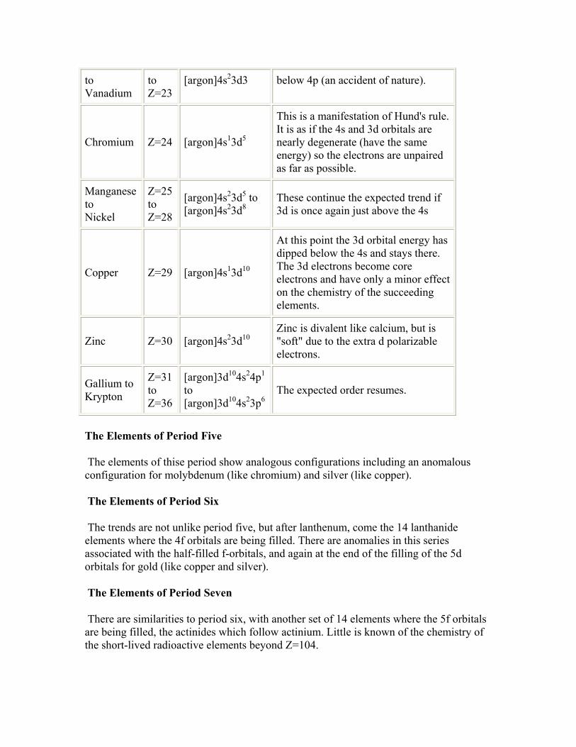
to Vanadium

to Z=23

[argon]4s23d3 below 4p (an accident of nature).

Chromium Z=24 [argon]4s13d5

This is a manifestation of Hund's rule. It is as if the 4s and 3d orbitals are nearly degenerate (have the same energy) so the electrons are unpaired as far as possible.

Manganese to Nickel

Z=25 to Z=28

[argon]4s23d5 to [argon]4s23d8

These continue the expected trend if 3d is once again just above the 4s

Copper Z=29 [argon]4s13d10

At this point the 3d orbital energy has dipped below the 4s and stays there. The 3d electrons become core electrons and have only a minor effect on the chemistry of the succeeding elements.

Zinc Z=30 [argon]4s23d10 Zinc is divalent like calcium, but is "soft" due to the extra d polarizable electrons.

Gallium to Krypton

Z=31 to Z=36

[argon]3d104s24p1 to [argon]3d104s23p6

The expected order resumes.

The Elements of Period Five

The elements of thise period show analogous configurations including an anomalous configuration for molybdenum (like chromium) and silver (like copper).

The Elements of Period Six

The trends are not unlike period five, but after lanthenum, come the 14 lanthanide elements where the 4f orbitals are being filled. There are anomalies in this series associated with the half-filled f-orbitals, and again at the end of the filling of the 5d orbitals for gold (like copper and silver).

The Elements of Period Seven

There are similarities to period six, with another set of 14 elements where the 5f orbitals are being filled, the actinides which follow actinium. Little is known of the chemistry of the short-lived radioactive elements beyond Z=104.

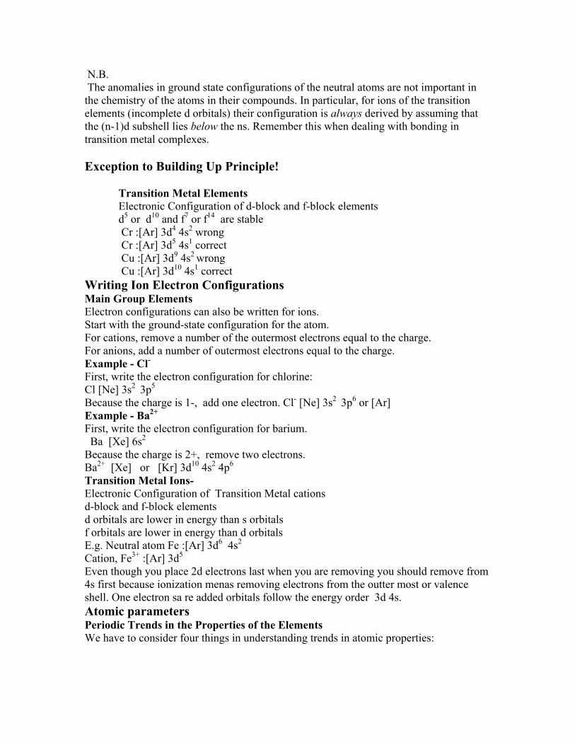
N.B. The anomalies in ground state configurations of the neutral atoms are not important in the chemistry of the atoms in their compounds. In particular, for ions of the transition elements (incomplete d orbitals) their configuration is always derived by assuming that the (n-1)d subshell lies below the ns. Remember this when dealing with bonding in transition metal complexes.

Exception to Building Up Principle!

Transition Metal Elements Electronic Configuration of d-block and f-block elements d5 or d10 and f7 or f14 are stable Cr :[Ar] 3d4 4s2 wrong Cr :[Ar] 3d5 4s1 correct Cu :[Ar] 3d9 4s2 wrong Cu :[Ar] 3d10 4s1 correct

Writing Ion Electron Configurations Main Group Elements Electron configurations can also be written for ions. Start with the ground-state configuration for the atom. For cations, remove a number of the outermost electrons equal to the charge. For anions, add a number of outermost electrons equal to the charge. Example - Cl- First, write the electron configuration for chlorine: Cl [Ne] 3s2 3p5 Because the charge is 1-, add one electron. Cl- [Ne] 3s2 3p6 or [Ar] Example - Ba2+ First, write the electron configuration for barium. Ba [Xe] 6s2 Because the charge is 2+, remove two electrons. Ba2+ [Xe] or [Kr] 3d10 4s2 4p6 Transition Metal Ions- Electronic Configuration of Transition Metal cations d-block and f-block elements d orbitals are lower in energy than s orbitals f orbitals are lower in energy than d orbitals E.g. Neutral atom Fe :[Ar] 3d6 4s2 Cation, Fe3+ :[Ar] 3d5 Even though you place 2d electrons last when you are removing you should remove from 4s first because ionization menas removing electrons from the outter most or valence shell. One electron sa re added orbitals follow the energy order 3d 4s. Atomic parameters Periodic Trends in the Properties of the Elements We have to consider four things in understanding trends in atomic properties:

1. The different interpenetrations of the atomic orbitals. Overall "sizes" are a function of R(r)2 while orientation is a function of Θ(θ)2Φ(φ)2.

2. We know the filling order. 3. We can estimate effective nuclear charges.

We also know the occupancy of the individual orbitals which may come into play.

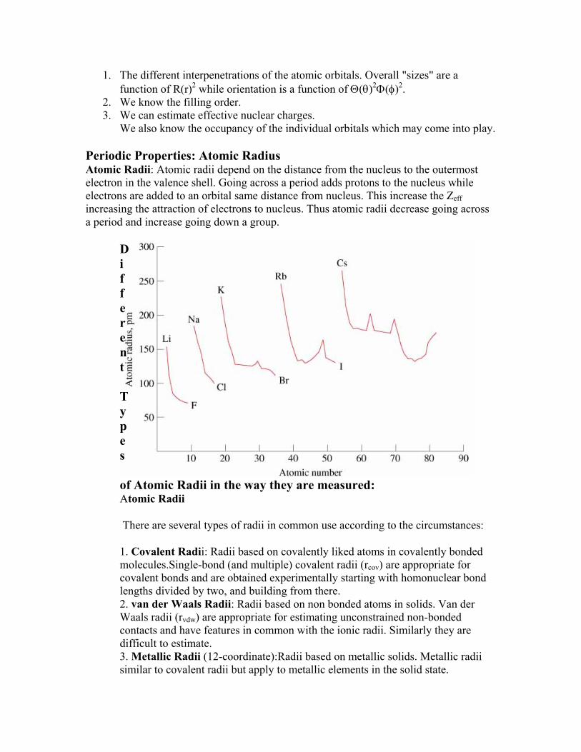
Periodic Properties: Atomic Radius Atomic Radii: Atomic radii depend on the distance from the nucleus to the outermost electron in the valence shell. Going across a period adds protons to the nucleus while electrons are added to an orbital same distance from nucleus. This increase the Zeff increasing the attraction of electrons to nucleus. Thus atomic radii decrease going across a period and increase going down a group.

Different Types of Atomic Radii in the way they are measured: Atomic Radii

There are several types of radii in common use according to the circumstances:

1. Covalent Radii: Radii based on covalently liked atoms in covalently bonded molecules.Single-bond (and multiple) covalent radii (rcov) are appropriate for covalent bonds and are obtained experimentally starting with homonuclear bond lengths divided by two, and building from there. 2. van der Waals Radii: Radii based on non bonded atoms in solids. Van der Waals radii (rvdw) are appropriate for estimating unconstrained non-bonded contacts and have features in common with the ionic radii. Similarly they are difficult to estimate. 3. Metallic Radii (12-coordinate):Radii based on metallic solids. Metallic radii similar to covalent radii but apply to metallic elements in the solid state.

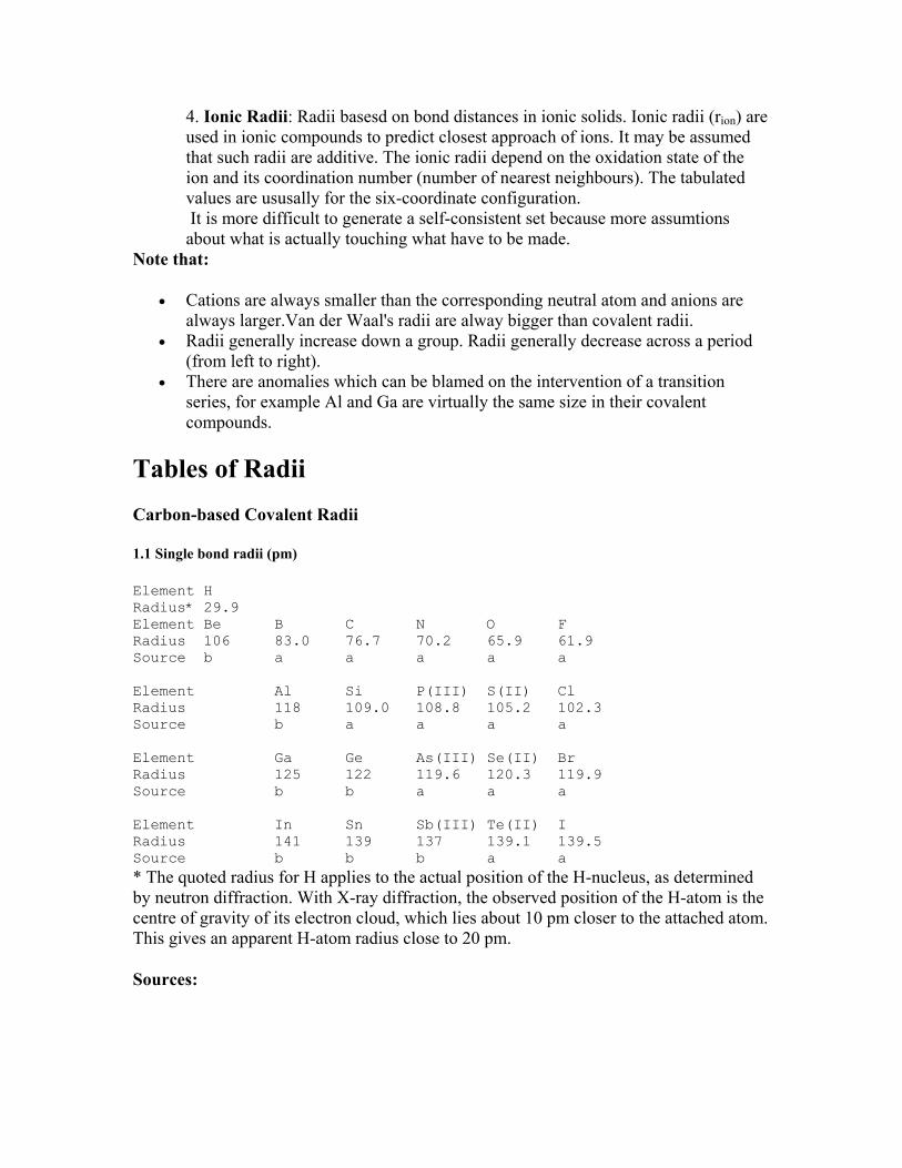
4. Ionic Radii: Radii basesd on bond distances in ionic solids. Ionic radii (rion) are used in ionic compounds to predict closest approach of ions. It may be assumed that such radii are additive. The ionic radii depend on the oxidation state of the ion and its coordination number (number of nearest neighbours). The tabulated values are ususally for the six-coordinate configuration. It is more difficult to generate a self-consistent set because more assumtions about what is actually touching what have to be made.

Note that:

• Cations are always smaller than the corresponding neutral atom and anions are always larger.Van der Waal's radii are alway bigger than covalent radii.

• Radii generally increase down a group. Radii generally decrease across a period (from left to right).

• There are anomalies which can be blamed on the intervention of a transition series, for example Al and Ga are virtually the same size in their covalent compounds.

Tables of Radii Carbon-based Covalent Radii

1.1 Single bond radii (pm)

Element H Radius* 29.9 Element Be B C N O F Radius 106 83.0 76.7 70.2 65.9 61.9 Source b a a a a a Element Al Si P(III) S(II) Cl Radius 118 109.0 108.8 105.2 102.3 Source b a a a a Element Ga Ge As(III) Se(II) Br Radius 125 122 119.6 120.3 119.9 Source b b a a a Element In Sn Sb(III) Te(II) I Radius 141 139 137 139.1 139.5 Source b b b a a * The quoted radius for H applies to the actual position of the H-nucleus, as determined by neutron diffraction. With X-ray diffraction, the observed position of the H-atom is the centre of gravity of its electron cloud, which lies about 10 pm closer to the attached atom. This gives an apparent H-atom radius close to 20 pm.

Sources:

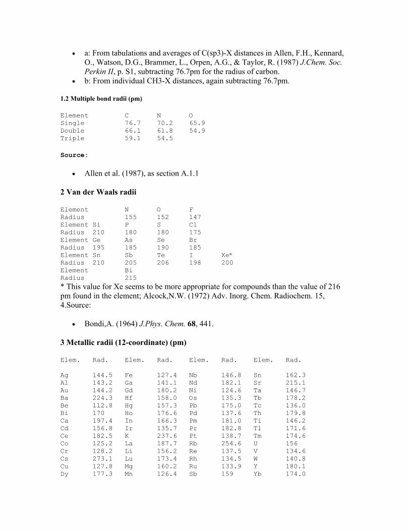
• a: From tabulations and averages of C(sp3)-X distances in Allen, F.H., Kennard, O., Watson, D.G., Brammer, L., Orpen, A.G., & Taylor, R. (1987) J.Chem. Soc. Perkin II, p. S1, subtracting 76.7pm for the radius of carbon.

• b: From individual CH3-X distances, again subtracting 76.7pm.

1.2 Multiple bond radii (pm)

Element C N O Single 76.7 70.2 65.9 Double 66.1 61.8 54.9 Triple 59.1 54.5

Source:

• Allen et al. (1987), as section A.1.1

2 Van der Waals radii

Element N O F Radius 155 152 147 Element Si P S Cl Radius 210 180 180 175 Element Ge As Se Br Radius 195 185 190 185 Element Sn Sb Te I Xe* Radius 210 205 206 198 200 Element Bi Radius 215 * This value for Xe seems to be more appropriate for compounds than the value of 216 pm found in the element; Alcock,N.W. (1972) Adv. Inorg. Chem. Radiochem. 15, 4.Source:

• Bondi,A. (1964) J.Phys. Chem. 68, 441.

3 Metallic radii (12-coordinate) (pm)

Elem. Rad. Elem. Rad. Elem. Rad. Elem. Rad. Ag 144.5 Fe 127.4 Nb 146.8 Sn 162.3 Al 143.2 Ga 141.1 Nd 182.1 Sr 215.1 Au 144.2 Gd 180.2 Ni 124.6 Ta 146.7 Ba 224.3 Hf 158.0 Os 135.3 Tb 178.2 Be 112.8 Hg 157.3 Pb 175.0 Tc 136.0 Bi 170 Ho 176.6 Pd 137.6 Th 179.8 Ca 197.4 In 166.3 Pm 181.0 Ti 146.2 Cd 156.8 Ir 135.7 Pr 182.8 Tl 171.6 Ce 182.5 K 237.6 Pt 138.7 Tm 174.6 Co 125.2 La 187.7 Rb 254.6 U 156 Cr 128.2 Li 156.2 Re 137.5 V 134.6 Cs 273.1 Lu 173.4 Rh 134.5 W 140.8 Cu 127.8 Mg 160.2 Ru 133.9 Y 180.1 Dy 177.3 Mn 126.4 Sb 159 Yb 174.0

Er 175.7 Mo 140.0 Sc 164.1 Zn 139.4 Eu 204.2 Na 191.1 Sm 180.2 Zr 160.2 Source:Teatum,E., Gschneidner,K., & Waber,J. (1960) Compilation of calculated data useful in predicting metallurgical behaviour of the elements in binary alloy systems, LA-2345, Los Alamos Scientific Laboratory.

4 Ionic radii

4.1 Cation radii (6-coordinate) (pm) Radii are quoted for common oxidation states up to +3 (4 for Hf, Th, Ti, U, and Zr). Elem. Rad. Elem. Rad. Elem. Rad. Elem. Rad. Ag(+1) 129 Er(+3) 103.0 Mn(+3) 72/78.5* Ta(+3) 86 Al(+3) 67.5 Eu(+2) 131 Mo(+3) 83 Tb(+3) 106.3 Au(+1) 151 Eu(+3) 108.7 Na(+1) 116 Th(+4) 108 Au(+3) 99 Fe(+2) 75/92.0* Nb(+3) 86 Ti(+2) 100 Ba(+2) 149 Fe(+3) 69/78.5* Nd(+3) 112.3 Ti(+3) 81.0 Be(+2) 59 Ga(+3) 76.0 Ni(+2) 83.0 Ti(+4) 74.5 Bi(+3) 117 Gd(+3) 107.8 Pb(+2) 133 Tl(+1) 164 Ca(+2) 114 Hf(+4) 85 Pd(+2) 100 Tl(+3) 102.5 Cd(+2) 109 Hg(+1) 133 Pm(+3) 111 Tm(+3) 102.0 Ce(+3) 115 Hg(+2) 116 Pr(+3) 113 U(+3) 116.5 Ce(+4) 101 Ho(+3) 104.1 Pt(+2) 94 U(+4) 103 Co(+2) 79/88.5* In(+3) 94.0 Rb(+1) 166 V(+2) 93 Co(+3) 68.5/75* Ir(+3) 82 Rh(+3) 80.5 V(+3) 78.0 Cr(+2) 87/94* K(+1) 152 Ru(+3) 82 Y(+3) 104.0 Cr(+3) 75.5 La(+3) 117.2 Sb(+3) 90 Yb(+2) 116 Cs(+1) 181 Li(+1) 90 Sc(+3) 88.5 Yb(+3) 100.8 Cu(+1) 91 Lu(+3) 100.1 Sm(+3) 109.8 Zn(+2) 88.0 Cu(+2) 87 Mg(+2) 86.0 Sr(+2) 132 Zr(+4) 86 Dy(+3) 105.2 Mn(+2) 81/97.0* * Low spin and high spin values (section 8.2.3) Source: Shannon,R.D. (1976) `Revised effective ionic radii in halides and chalcogenides',Acta Cryst.A32, 751. This includes further oxidation states and coordination numbers.

Anion radii (6-coordinate) (pm)

Elem. Rad. Elem. Rad. Cl(-1) 167 O(-2) 126 Br(-1) 182 S(-2) 170 F(-1) 119 Se(-2) 184 I(-1) 206 Te(-2) 207

Periodic Properties: Ionization Energy It is defined as the energy required to remove the outermost electron from a gaseous atom. A "gaseous atom" means an atom that is all by itself, not hooked up to others in a solid or a liquid. When enough energy is added to an atom the outermost electron can use that energy to pull away from the nucleus completely (or be pulled, if you want to put it that way), leaving behind a positively charged ion. That is why it's called ionization, one

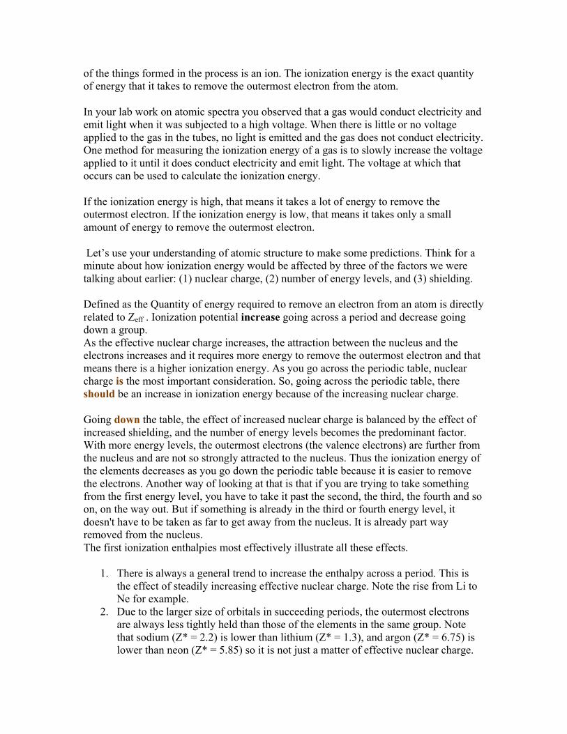
of the things formed in the process is an ion. The ionization energy is the exact quantity of energy that it takes to remove the outermost electron from the atom.

In your lab work on atomic spectra you observed that a gas would conduct electricity and emit light when it was subjected to a high voltage. When there is little or no voltage applied to the gas in the tubes, no light is emitted and the gas does not conduct electricity. One method for measuring the ionization energy of a gas is to slowly increase the voltage applied to it until it does conduct electricity and emit light. The voltage at which that occurs can be used to calculate the ionization energy.

If the ionization energy is high, that means it takes a lot of energy to remove the outermost electron. If the ionization energy is low, that means it takes only a small amount of energy to remove the outermost electron.

Let’s use your understanding of atomic structure to make some predictions. Think for a minute about how ionization energy would be affected by three of the factors we were talking about earlier: (1) nuclear charge, (2) number of energy levels, and (3) shielding.

Defined as the Quantity of energy required to remove an electron from an atom is directly related to Zeff . Ionization potential increase going across a period and decrease going down a group. As the effective nuclear charge increases, the attraction between the nucleus and the electrons increases and it requires more energy to remove the outermost electron and that means there is a higher ionization energy. As you go across the periodic table, nuclear charge is the most important consideration. So, going across the periodic table, there should be an increase in ionization energy because of the increasing nuclear charge.

Going down the table, the effect of increased nuclear charge is balanced by the effect of increased shielding, and the number of energy levels becomes the predominant factor. With more energy levels, the outermost electrons (the valence electrons) are further from the nucleus and are not so strongly attracted to the nucleus. Thus the ionization energy of the elements decreases as you go down the periodic table because it is easier to remove the electrons. Another way of looking at that is that if you are trying to take something from the first energy level, you have to take it past the second, the third, the fourth and so on, on the way out. But if something is already in the third or fourth energy level, it doesn't have to be taken as far to get away from the nucleus. It is already part way removed from the nucleus. The first ionization enthalpies most effectively illustrate all these effects.

1. There is always a general trend to increase the enthalpy across a period. This is the effect of steadily increasing effective nuclear charge. Note the rise from Li to Ne for example.

2. Due to the larger size of orbitals in succeeding periods, the outermost electrons are always less tightly held than those of the elements in the same group. Note that sodium (Z* = 2.2) is lower than lithium (Z* = 1.3), and argon (Z* = 6.75) is lower than neon (Z* = 5.85) so it is not just a matter of effective nuclear charge.

3. The estimation of effective nuclear charge is not sufficiently sensitive (using th above rules) to allow for the effect of changing subshell within a period. Note the drop from Be to B. There is another discontinuity at the half-filled p-subshell, e.g. nitrogen to oxygen, and less well defined ones at the half-filled d and f-subshellss. This occurs when pairing begins and electrons are forced into the same orbital.

Change in Ionization Moving Along a Period: The periodic nature of ionization energy is emphasized in this diagram. With each new period the ionization energy starts with a low value. Within each period you will notice that the pattern is really kind of a zigzag pattern progressing up as you go across the periodic table. The zigs and zags on that graph correspond to the sublevels in the energy levels. So far in this lesson we have presumed that all the electrons in the second energy level are pretty much the same. Two factors make that not completely true. One factor is that because s and p orbitals have different shapes, the electrons in p orbitals have more energy and are further from the nucleus. The other factor is that when electrons are paired up in an orbital, they repel one another somewhat. Those two factors account for the zigzag nature of the increase in ionization energy. Nevertheless, as a general trend, from left to right across the periodic table, ionization energy does increase. Also as you go down the periodic table, the ionization energy does decrease for the reasons given. These observations can be explained by looking at the electron configurations of these elements. The electron removed when a beryllium atom is ionized comes from the 2s orbital, but a 2p electron is removed when boron is ionized.

Be: [He] 2s2 B: [He] 2s2 2p1

The electrons removed when nitrogen and oxygen are ionized also come from 2p orbitals.

N: [He] 2s2 2p3 O: [He] 2s2 2p4

But there is an important difference in the way electrons are distributed in these atoms. Hund's rules predict that the three electrons in the 2p orbitals of a nitrogen atom all have the same spin, but electrons are paired in one of the 2p orbitals on an oxygen atom.

Hund's rules can be understood by assuming that electrons try to stay as far apart as possible to minimize the force of repulsion between these particles. The three electrons in the 2p orbitals on nitrogen therefore enter different orbitals with their spins aligned in the same direction. In oxygen, two electrons must occupy one of the 2p orbitals. The force of

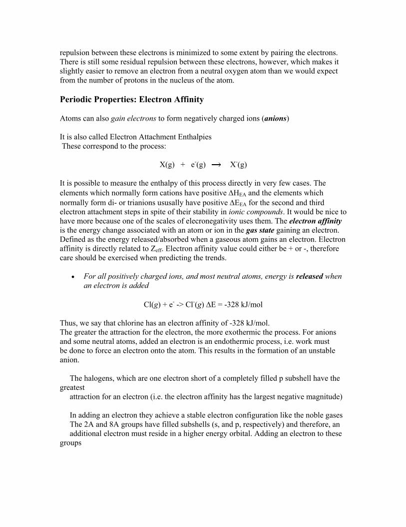
repulsion between these electrons is minimized to some extent by pairing the electrons. There is still some residual repulsion between these electrons, however, which makes it slightly easier to remove an electron from a neutral oxygen atom than we would expect from the number of protons in the nucleus of the atom.

Periodic Properties: Electron Affinity

Atoms can also gain electrons to form negatively charged ions (anions)

It is also called Electron Attachment Enthalpies These correspond to the process:

X(g) + e-(g) X-(g)

It is possible to measure the enthalpy of this process directly in very few cases. The elements which normally form cations have positive ∆HEA and the elements which normally form di- or trianions ususally have positive ∆EEA for the second and third electron attachment steps in spite of their stability in ionic compounds. It would be nice to have more because one of the scales of elecronegativity uses them. The electron affinity is the energy change associated with an atom or ion in the gas state gaining an electron. Defined as the energy released/absorbed when a gaseous atom gains an electron. Electron affinity is directly related to Zeff. Electron affinity value could either be + or -, therefore care should be exercised when predicting the trends.

• For all positively charged ions, and most neutral atoms, energy is released when an electron is added

Cl(g) + e- -> Cl-(g) ∆E = -328 kJ/mol

Thus, we say that chlorine has an electron affinity of -328 kJ/mol. The greater the attraction for the electron, the more exothermic the process. For anions and some neutral atoms, added an electron is an endothermic process, i.e. work must be done to force an electron onto the atom. This results in the formation of an unstable anion.

The halogens, which are one electron short of a completely filled p subshell have the greatest attraction for an electron (i.e. the electron affinity has the largest negative magnitude)

In adding an electron they achieve a stable electron configuration like the noble gases The 2A and 8A groups have filled subshells (s, and p, respectively) and therefore, an additional electron must reside in a higher energy orbital. Adding an electron to these groups

is an endothermic process

Across a period, value of electron affinity generally decrease (going from a small positive value to a larger negative value represents a decrease) Going down a group Electron Affinity values increase. Electronegativity: These measure the tendency for one element of a bonded pair to attract the electrons associated with the bond to itself. The polarity of a bond, that is its ionic character is assessed by comparing the two electronegativities of the two bonded atoms. It is also possible to assign an electronegativity to a chemical group e.g. CH3. In LiH molecule, it would seem that the bonding orbital places more electron density on the hydrogen than on the lithium since the orbital shape describes the probability of finding the electrons. As a result, the hydrogen end of the moelcule would be slightly negative and the lithium end would be slightly positive.This situation is called a polar bond in which the electrons

in the bond are being shared, but not equally shared.

In almost every case in which a bond is formed between two different atoms the resulting bond will be polar.

I In the 1930's, Linus Pauling (1901 - 1994), an American chemist who won the 1954 Nobel Prize, recognized that bond polarity resulted from the relative ability of atoms to attract electrons. Pauling devised a measure of this electron attracting power which he called

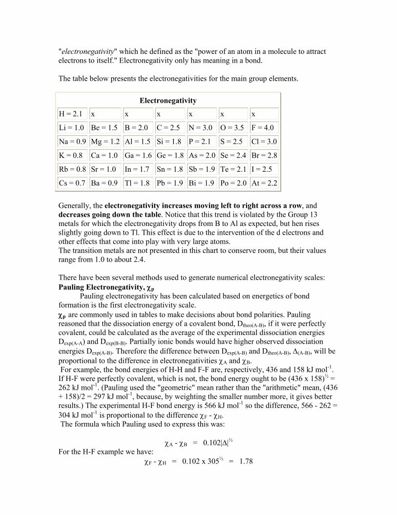
"electronegativity" which he defined as the "power of an atom in a molecule to attract electrons to itself." Electronegativity only has meaning in a bond.

The table below presents the electronegativities for the main group elements.

Electronegativity

H = 2.1 x x x x x x

Li = 1.0 Be = 1.5 B = 2.0 C = 2.5 N = 3.0 O = 3.5 F = 4.0

Na = 0.9 Mg = 1.2 Al = 1.5 Si = 1.8 P = 2.1 S = 2.5 Cl = 3.0

K = 0.8 Ca = 1.0 Ga = 1.6 Ge = 1.8 As = 2.0 Se = 2.4 Br = 2.8

Rb = 0.8 Sr = 1.0 In = 1.7 Sn = 1.8 Sb = 1.9 Te = 2.1 I = 2.5

Cs = 0.7 Ba = 0.9 Tl = 1.8 Pb = 1.9 Bi = 1.9 Po = 2.0 At = 2.2

Generally, the electronegativity increases moving left to right across a row, and decreases going down the table. Notice that this trend is violated by the Group 13 metals for which the electronegativity drops from B to Al as expected, but hen rises slightly going down to Tl. This effect is due to the intervention of the d electrons and other effects that come into play with very large atoms. The transition metals are not presented in this chart to conserve room, but their values range from 1.0 to about 2.4.

There have been several methods used to generate numerical electronegativity scales: Pauling Electronegativity, χp Pauling electronegativity has been calculated based on energetics of bond formation is the first electronegativity scale. χp are commonly used in tables to make decisions about bond polarities. Pauling reasoned that the dissociation energy of a covalent bond, Dtheo(A-B), if it were perfectly covalent, could be calculated as the average of the experimental dissociation energies Dexp(A-A) and Dexp(B-B). Partially ionic bonds would have higher observed dissociation energies Dexp(A-B). Therefore the difference between Dexp(A-B) and Dtheo(A-B), ∆(A-B), will be proportional to the difference in electronegativities χA and χB. For example, the bond energies of H-H and F-F are, respectively, 436 and 158 kJ mol-1. If H-F were perfectly covalent, which is not, the bond energy ought to be (436 x 158)½ = 262 kJ mol-1. (Pauling used the "geometric" mean rather than the "arithmetic" mean, (436 + 158)/2 = 297 kJ mol-1, because, by weighting the smaller number more, it gives better results.) The experimental H-F bond energy is 566 kJ mol-1 so the difference, 566 - 262 = 304 kJ mol-1 is proportional to the difference χF - χH. The formula which Pauling used to express this was:

χA - χB = 0.102|∆|½ For the H-F example we have:

χF - χH = 0.102 x 305½ = 1.78

Pauling assigned the value for χF as 4.00 which gives χH = 4.00 - 1.78 = 2.22. This method is also dependent on lots of experimental data, but the data is much more accessible.

Mulliken Electronegativity, χM This scale is based on the average of the ionization enthalpy and the negative of the electron attachment enthalpy. R.S. Mulliken proposed an electronegativity scale in which the Mulliken electronegativity, χM is related to the electron affinity EAv (a measure of the tendency of an atom to form a negative species) and the ionization potential IEv (a measure of the tendency of an atom to form a positive species) by the equation:

χM = (∆HIE - ∆HEA)/2

A strong tendency to gain electrons is characterized by a large negative∆HEA and a large positive ∆HIE will go with a reluctance to lose electrons, both of which will contribute to an element showing a large electronegativity. The method makes gfreat sense but is limited by the lack of electron attachment enthalpy data.

∆HIE - ∆HEA depends on specific valence state - so for trigonal boron compounds, a values of electronegativity can be defined for sp2 hybrid orbitals. If the values of IE and EA are in units of MJ mol-1, then the Mulliken electronegativity χM can be expressed on the Pauling scale by the relationship:

χp = 1.35 χM1/2 - 1.37

The Allred-Rochow electronegativity- χAR. The underlying theoretical concept is that an electron close to the surface of an atom i.e. a bonding electron is held there by the effective nuclear charge it experiences, and the force resisting its removal is given by:

Force = (Zeffe)(e)/4πr2εo where r is the distance between the electron and the nucleus (covalent radius) e is the charge on an electron Zeff is the charge effective at the electron due to the nucleus and its surrounding electrons. εo is the permitivity. The quantity Zeff/r2 correlates well with Pauling electronegativities and the two scales can be made to coincide by expressing the Allred-Rochow electronegativity as:

χAR = 0.359(Z*/r2) + 0.744 Assuming the electronegativity is proportional to this force, and adding constants to bring the Allred-Rochow scale into correspondence with the Pauling scale (i.e. F = 4.00 and H = 2.22) gives: The Allen Scale This scale, which is designed only for the representative (main group) elements, comes

back to the use of ionization enthalpy data. In this case the weighted average ∆HIE for the s and p valence electrons, obtained from (atomic) spectroscopic data is used:

χspec = (mεs + nεp)/(m + n)

where n and m are the numbers of s and p electrons, respectively. Allen's numbers do not differ much from the other scales.

Polarizability

The ease with which the charge distribution in a molecule can be distorted by an external electric field is called its polarizability ('squashiness' of its e- cloud). The greater the polarizability, the more easily its e- cloud can be distorted. Larger molecules tend to have greater polarizabilities - they have more e- and their e- are further from the nuclei e.g. I2 is more polarizable than F2. Measures the ease of distortion of an atom in an electric field. If the frontier orbitals are not widely separated, then the atom will be more polarizable. This happens more for heavier elements. Atoms resistant to polariation are "hard", while atoms which are easily polarized are "soft".