Rotation Curve Measurement using Cross-Correlation 1

Elizabeth J. Barton2, Sheila J. Kannappan, Michael J. Kurtz, Margaret J. GellerHarvard-Smithsonian Center for Astrophysics

ABSTRACT

Longslit spectroscopy is entering an era of increased spatial and spectral resolutionand increased sample size. Improved instruments reveal complex velocity structurethat cannot be described with a one-dimensional rotation curve, yet samples are toonumerous to examine each galaxy in detail. Therefore, one goal of rotation curvemeasurement techniques is to flag cases in which the kinematic structure of the galaxyis more complex than a single-valued curve.

We examine cross-correlation as a technique that is easily automated and worksfor low signal-to-noise spectra. We show that the technique yields well-defined errorswhich increase when the simple spectral model (template) is a poor match to the data,flagging those cases for later inspection.

We compare the technique to the more traditional, parametric technique ofsimultaneous emission line fitting. When the line profile at a single slit position isnon-Gaussian, the techniques disagree. For our model spectra with two well-separatedvelocity components, assigned velocities from the two techniques differ by up to ∼52 %of the velocity separation of the model components. However, careful use of the errorstatistics for either technique allows one to flag these non-Gaussian spectra.

Subject headings: methods: data analysis — techniques: radial velocities

1. Introduction

Spatially resolved optical spectroscopy became a tool for studying the dynamics of externalgalaxies when Pease (1918) observed rotation in the inner part of M31 (Rubin 1995). Later,Babcock (1939) effectively measured an optical “rotation curve” of M31 by measuring velocities ofindividual nebular regions separately. Although required exposure times were very long, somewhatlarger samples of rotation curves were amassed in the inner portions of galaxies (Burbidge &

1Observations reported in this paper were obtained at the Multiple Mirror Telescope Observatory, a facility

operated jointly by the University of Arizona and the Smithsonian Institution.

2present address: National Research Council of Canada, Herzberg Institute of Astrophysics, Dominion

Astrophysical Observatory, 5071 W. Saanich Road, RR5, Victoria, BC, Canada V8X 4M6

brought to you by COREView metadata, citation and similar papers at core.ac.uk

provided by CERN Document Server

– 2 –

Burbidge 1975), and finally in the outer regions. Now, optical rotation curves of nearby galaxiescan be measured with brief exposure times, enabling the construction of very large samples ofrotation curves for statistical purposes (e.g. Rubin et al. 1985; Mathewson, Ford & Buchhorn1992; Courteau 1997).

Improvements in the spatial and velocity resolution of optical spectrographs have revealedcomplex velocity structure in both elliptical and spiral galaxies. The phenomena include distinct,nuclear kinematic components in spiral galaxies (e.g. Marziani et al. 1994; Rubin, Kenney& Young 1997; Bureau & Freeman 1999), and in the cores of elliptical galaxies (e.g. Franx,Illingworth & Heckman 1989).

The physics behind the complex velocity structure seen in emission lines is difficult to unravel.Although there are numerous techniques for inferring the line-of-sight velocity structure of a stellarsystem from a non-Gaussian absorption line profile (e.g. Rix & White 1992; van der Marel &Franx 1993; Merrifield & Kuijken 1994), the analogous measurements for emission-line kinematicsare largely unconstrained. Emitting regions have non-uniform internal velocity structure whichcomplicates the structure of the emission lines (e.g. from individual HII regions; Osterbrock 1989).

To date, estimates of the true kinematic structure of galaxies with complex emission lineprofiles are largely qualitative (e.g. Rubin et al. 1997), and most rotation curve reductionsassign a single velocity at each slit position. In most longslit, emission-line spectroscopic studies,velocities are computed with some form of Gaussian line fitting (e.g. Keel 1996) or line centroidingor peak fitting (e.g. Courteau 1997; Rubin et al. 1997), of either the brightest emission line or asubset of emission lines simultaneously. Mathewson et al. (1992) and Marquez & Moles (1996) usecross-correlation to measure rotation curves, but without detailed description of their technique.

In this era of large, high-quality rotation curve samples, techniques for rotation curvereduction need to be re-examined. Here, we evaluate a little-used but easily-implementedtechnique for longslit rotation curve reduction, cross correlation. We give special attention tothe fact that each aperture along the slit may contain emission from multiple velocities. Thetechnique (1) yields a well-defined response to all line profiles — the velocity and error have aclear physical relationship to the observed line profile, (2) is accurate when extracting redshifts oflow signal-to-noise (S/N) spectra, and (3) is easily automated. Focusing on (1), we compare thetechnique to the fundamentally different, parametric technique of Gaussian line fitting.

We test the techniques for redshift measurement in a controlled manner, using model spectrawith varied properties. Our intent is to highlight the most relevant features of the techniques,not to explore parameter space exhaustively. In § 2, we describe two techniques which representfundamentally different approaches, cross-correlation and Gaussian fitting. In § 3, we test themwith single-aperture Gaussian and two-component line profiles, to illustrate that when the lineprofile is non-Gaussian, different techniques can yield different results, and to track the errorbehavior. In § 4, we apply the techniques to two-dimensional model rotation curves to illustratethe error behavior in situations which commonly arise in longslit spectroscopy. In § 5 we briefly

– 3 –

discuss applying cross-correlation to longslit spectral data. We conclude in § 6.

2. Exploring Cross-Correlation and Simultaneous Emission Line Fitting

We evaluate an effective technique for redshift measurement, cross-correlation (XC), whichis little-used for emission-line measurements. We compare it to an alternative technique,simultaneous emission line fitting (SEMLF; as in Keel 1996). The techniques represent the twofundamentally different approaches to these measurements. SEMLF is parametric, involvingmodeling the emission lines and fitting for the parameters. XC is non-parametric in the sensethat we do not fit for parameters, although the technique does involve assumptions — we use amodel spectrum for a template in the computation. Our comparison of the techniques shows thatwhen a single-velocity measurement is ill-defined, as when components at two separate velocitiescontribute to the spectrum, different approaches yield different results. Thus, these cases must beflagged and dealt with separately for a proper characterization of the velocity structure of eachgalaxy.

Both techniques can be reliably automated, although SEMLF requires some fine-tuning, asdoes XC in the low S/N case. XC is easily implemented with xcsao (see Kurtz & Mink 1998),within the IRAF (Tody 1986; 1993) environment. We use a version of SEMLF based on thatof Kannappan et al. (1999) implemented with IDL (Landsman 1995). Both techniques apply aspecific model to the data — they assume a pre-determined line profile which is usually a Gaussian.However, longslit observations are designed to detect spatially separated components at differentvelocities. These components may broaden line profiles, or may turn them into double-peakedprofiles. When the Gaussian model is not a good representation of the data, the techniques willproduce different results. Below, we explore results for Gaussian and double-Gaussian profiles.

We use artificial emission-line spectra with noise to explore and compare the XC and SEMLFtechniques. We construct the spectra with the linespec task in RVSAO, and add noise withmknoise in NOAO.ARTDATA. Figure 1 shows the basic spectrum, a set of 5 Gaussian profilescentered at the major emission lines, Hα, [SII] and [NII], redshifted to 4000.0 km s−1. We chooselinewidths typical of spectra taken with a 1200 g/mm grating and a narrow (1.0′′) slit — Hα

has a full width at half maximum (FWHM) of 2.3 A = 104 km s−1. The other lines satisfy2.26 ≤ FWHM ≤ 2.50 A. To add the noise, we assume a gain of 1.5 e−/DN and a read noise of7.0 e−. Although the continuum S/N ratio is not defined in these model spectra, the effectivesignal-to-noise ratio of the Hα line is very large in many of them: the Hα signal in the spectrum inFig. 1 is ∼2300 e− over 5 pixels, so the S/N ratio in Hα is ∼45. Although we vary the S/N ratio inthe model spectra in the examples of § 3.1, most of the other test spectra have comparably largeS/N ratios. The discrete pixel sampling scale is ∼22 km s−1.

– 4 –

2.1. The Cross-Correlation Technique

Kurtz & Mink (1998) describe cross-correlation exhaustively for application to redshiftsurveys, using the task xcsao in the RVSAO package, within the IRAF environment (Tody 1986,1993). They include template construction and error analysis in their discussion. We apply theXC technique using xcsao in RVSAO, according to the procedure that would be used for actualdata (excluding bias subtraction, flat-fielding, wavelength calibration, and cosmic ray removal).We construct the template based on the median widths and relative heights of the “emissionlines” in a large ensemble of model spectra, just as we would for actual data (see § 4). Becausethe high-resolution models are undersampled relative to the optimal sampling rate for xcsao, wemust adjust the rebinning in xcsao, by using both linear and spline3 interpolation and choosingthe best result based on the r statistic.

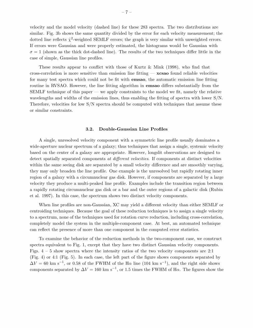
Fig. 2 shows a sample peak in the correlation function, which xcsao fits to find the velocityfor the spectrum in Fig. 1. Because the sample spectrum has a very large S/N ratio and anearly-perfect Gaussian profile, the peak is well-defined and the redshift, 4001.1 ± 0.4 km s−1, isclose to the input model value of 4000 km s−1.

Cross-correlation errors include the effects of spectrum/template mismatch, and thereforehave a clear relationship to the spectral profile. The internal error estimator of Kurtz & Mink(1998) follows from the discussion in Tonry & Davis (1979, TD hereafter), with the additionalassumption that the noise is sinusoidal. xcsao computes an error of 3

8ω

1+r , where ω is theFWHM of the correlation peak and r, defined by TD, is a measure of the noise based on theantisymmetric part of the correlation function. TD assume that the (symmetric) template,convolved with a simple symmetric function, is a noise-free spectral match to the object — that allspectrum/template mismatch is the result of noise. Under these assumptions, the antisymmetricpart of the correlation function yields a measure of the height of the average noise peak — agalaxy with symmetric line profiles, cross-correlated with a template with symmetric line profiles,has noise and no signal in the antisymmetric part of its correlation function. Thus, the error thatxcsao computes is the shift in the correlation peak center that would result from a spurious noisepeak, where 3

8ω is the average distance to the nearest noise peak and, with the assumptions ofTD, r is an estimate of the height of the true correlation peak divided by of the height of theaverage noise peak.

If r is small, there are spurious peaks in the correlation function comparable to or exceedingthe highest peak. xcsao is likely to fit one of these spurious peaks instead of the true peak; thenthe computed velocity is arbitrarily far from the true velocity, much farther than the formal errorindicates. Thus, r is a measure of the reliability of the redshift. Kurtz & Mink (1998) requirer > 3.0 for automatic acceptance of the extracted redshift. However, redshifts with r < 3.0 canbe used in longslit reduction because there are data in neighboring apertures. If xcsao fits thewrong peak, the redshift will appear discrepant from neighboring apertures and the reduction canbe checked manually, or rejected.

– 5 –

If the template has a single velocity component, the assumptions underlying the errorestimator are incorrect for spectra with multiple components at different velocities. In thismultiple-component case, spectrum/template mismatch results from noise and from additionalpeaks in the spectrum at different velocities. The mismatch generally appears in the antisymmetricpart of the correlation function, and r measures this template mismatch. Thus r becomes ameasure of how well the template fits the spectrum. Low r values indicate a poor fit, and result inlarge error. ω also reflects additional nearby velocity components; an additional nearby componentresults in a wider correlation peak, a larger ω and a larger error. Therefore, additional velocitycomponents enlarge XC errors significantly. Below, we explore this effect using model spectra.

Kurtz & Mink (1998) find that 38

ω1+r systemically over or underestimates nuclear redshift

errors by ∼20 %. For large redshift surveys consisting of nuclear spectra reduced uniformly witha single template, ω remains roughly constant. In that case, error calibration can be applied toeliminate the discrepancy. Kurtz & Mink (1998) solve for a template-dependent constant, k, wherethe true error is then k

1+r .

However, in longslit spectroscopy, where multiple-velocity spectra abound, ω is not constant.Throughout this paper, we use 3

8ω

1+r to estimate XC errors. We recommend computing errorsproportional to ω

1+r for all longslit reduction implemented with XC, because ω reflects the presenceof multiple velocity components and wide velocity components.

2.2. The SEMLF Technique

The major steps involved in SEMLF reduction are similar to the steps required to implementcross-correlation, except that we measure velocities by fitting single-Gaussian functions to themajor emission lines simultaneously, when the lines are detected at ≥ 3σ. All spectra reducedwith the SEMLF program were first transformed to log(λ) space using the task transform in theLONGSLIT package of IRAF, with an artificial calibration lamp image. In our implementationof SEMLF, the relative wavelengths are fixed and the linewidths are constrained to be the samevalue for each line; the overall linewidth and each individual peak height may vary. We derive theformal model-dependent errors from χ2-minimization fitting using the Gaussian model (Press etal. 1992).

When the minimal χ2 6= N ± √N , where N is the number of degrees of freedom in thefit, the formal errors cannot be justified rigorously. Press et al. (1992) emphasize that theseerrors are unsuitable when a model is an incorrect representation of the data. Finding the trueerrors requires other methods (e.g. Monte Carlo simulation) which are usually computationallyexpensive. Authors generally compute errors that account for photon statistics; some errorcalculations are independent of profile shape (Courteau 1997 uses the weighted mean) and/orinclude line widths (Keel 1996). However, these errors do not include mismatch between the dataand a basic model that in every case assumes a single, well-defined velocity. Here, we attempt

– 6 –

to partially account for this mismatch, taking an approach guided by the analogy between XCerrors and the error derived from weighting by the reduced χ2, because χ2 is an estimator ofthe suitability of the Gaussian model and reflects irregular line profiles. Although the procedureis not rigorously justified, we consider weighted errors as a computationally convenient way ofachieving an estimate of the proper error behavior; below, we multiply the error by the reducedχ2 = χ2/N . We demonstrate that the weighted errors display the expected error behavior and aresimilar to the XC errors. This similarity arises because both the XC 1

1+r statistic and the SEMLFχ2 are based on the cross product of the object and model spectra divided by an estimator of thevariance. The formal SEMLF error performs the same function as the width factor (3

8ω) in xcsao;it provides a scale by which to multiply the goodness of fit measure (χ2 for SEMLF, 1

1+r for XC)in order to estimate the uncertainty of the measurement.

The 3σ cutoff of SEMLF is analogous to imposing a lower limit on r in the XC technique.The limit is somewhat arbitrary and could be modified. In general, we do not modify the limit inour tests, so these tests do not directly compare the effectiveness of the two techniques on verylow S/N spectra.

We apply the SEMLF technique to the spectrum of Fig. 1, with a redshift of 4000 km s−1. Theresulting fit, with a velocity and weighted error of 4000.9 ± 0.5 km s−1, is nearly indistinguishablefrom the spectrum. Thus, both SEMLF and XC find the correct velocity of the line profiles whenthey are Gaussian (with large S/N ratios). SEMLF measures the proper error in the Gaussiancase; thus SEMLF, used with calibration spectra consisting of Gaussian line profiles, provides onemethod of calibrating the XC error when necessary.

3. Behavior of the Two Techniques for One-Dimensional Spectra

In the following sections, we explore the behavior of XC and SEMLF. We use one-dimensionalspectra with varying line profiles. We fix the emission line ratios to standard HII region valuessimilar to the XC template. Later, we consider two-dimensional spectra which mimic differentfeatures of galaxy rotation curves, including varying emission-line ratios. All models match theresolution of the data described in § 3. However, most of the model spectra have larger SNR’s,and therefore much larger r values, than typical rotation curve data.

3.1. Gaussian Line Profiles

We apply XC and SEMLF to a set of 400 single-Gaussian spectra identical to Fig. 1, exceptthat Hα S/N ratios vary from ∼54 to < 1. XC finds a velocity with r ≥ 1.5 for 297 of the spectra;SEMLF finds a redshift for 285 using the 3σ cutoff; we use the 283 spectra with results from bothtechniques for our analysis. Fig. 3a shows a histogram of the difference between the XC velocityand the input model velocity (solid line), superimposed on the difference between the SEMLF

– 7 –

velocity and the model velocity (dashed line) for these 283 spectra. The two distributions aresimilar. Fig. 3b shows the same quantity divided by the error for each velocity measurement; thedotted line reflects χ2-weighted SEMLF errors; the graph is very similar with unweighted errors.If errors were Gaussian and were properly estimated, the histograms would be Gaussian withσ = 1 (shown as the thick dot-dashed line). The results of the two techniques differ little in thecase of simple, Gaussian line profiles.

These results appear to conflict with those of Kurtz & Mink (1998), who find thatcross-correlation is more sensitive than emission line fitting — xcsao found reliable velocitiesfor many test spectra which could not be fit with emsao, the automatic emission line fittingroutine in RVSAO. However, the line fitting algorithm in emsao differs substantially from theSEMLF technique of this paper — we apply constraints to the model we fit, namely the relativewavelengths and widths of the emission lines, thus enabling the fitting of spectra with lower S/N.Therefore, velocities for low S/N spectra should be computed with techniques that assume theseor similar constraints.

3.2. Double-Gaussian Line Profiles

A single, unresolved velocity component with a symmetric line profile usually dominates awide-aperture nuclear spectrum of a galaxy; thus techniques that assign a single, systemic velocitybased on the center of a galaxy are appropriate. However, longslit observations are designed todetect spatially separated components at different velocities. If components at distinct velocitieswithin the same seeing disk are separated by a small velocity difference and are smoothly varying,they may only broaden the line profile. One example is the unresolved but rapidly rotating innerregion of a galaxy with a circumnuclear gas disk. However, if components are separated by a largevelocity they produce a multi-peaked line profile. Examples include the transition region betweena rapidly rotating circumnuclear gas disk or a bar and the outer regions of a galactic disk (Rubinet al. 1997). In this case, the spectrum shows two distinct velocity components.

When line profiles are non-Gaussian, XC may yield a different velocity than either SEMLF orcentroiding techniques. Because the goal of these reduction techniques is to assign a single velocityto a spectrum, none of the techniques used for rotation curve reduction, including cross-correlation,completely model the system in the multiple-component case. At best, an automated techniquecan reflect the presence of more than one component in the computed error statistics.

To examine the behavior of the reduction methods in the two-component case, we constructspectra equivalent to Fig. 1, except that they have two distinct Gaussian velocity components.Figs. 4 – 5 show spectra where the intensity ratios of the two velocity components are 2:1(Fig. 4) or 4:1 (Fig. 5). In each case, the left part of the figure shows components separated by∆V = 60 km s−1, or 0.58 of the FWHM of the Hα line (104 km s−1), and the right side showscomponents separated by ∆V = 160 km s−1, or 1.5 times the FWHM of Hα. The figures show the

– 8 –

“spectrum” around Hα (solid line) and the SEMLF fit (long-dashed line), along with the outputXC (dashed vertical line) and SEMLF (dotted vertical line) velocities. Note that when the velocityresolution differs from the model spectra we present (the FWHM of Hα is 104 km s−1), ∆V mustbe scaled to compare with our results.

In Fig. 4a, the two separate components are not visible as separate peaks. SEMLF andXC yield very similar results. In Fig. 4b, ∆V = 160 km s−1 — two distinct peaks are visible.The SEMLF technique fits one wide Gaussian to the two components. In contrast, XC finds avelocity closer to the stronger peak. The XC error increases by a factor of ∼16 over the resultin Fig. 4a, signaling the presence of the two distinct components. Appropriately, r decreasessubstantially, from 192 to 14, and and ω increases from 147 to 182. The SEMLF “formal” error inthe ∆V = 160 km s−1 case is only ∼ 2 times larger than in the ∆V = 60 km s−1 case, but the χ2

– weighted error is ∼23 times larger.

We note a similar trend for the spectral components with a larger flux ratio (4:1) in Fig. 5a(∆V = 60 km s−1) to Fig. 5b (∆V = 160 km s−1), except that both techniques fit close to thevelocity of the brighter peak (4720 km s−1). In Fig. 5b, SEMLF primarily fits the brighter peak,and the secondary peak, which does displace the resulting line profile, is not strongly reflected inthe unweighted error. On the other hand, the XC error and the SEMLF weighted error are ∼5and 6 times larger, respectively, than the errors in Fig. 5a, indicating model mismatch. Again, r

decreases substantially from 164 to 29; ω stays roughly the same.

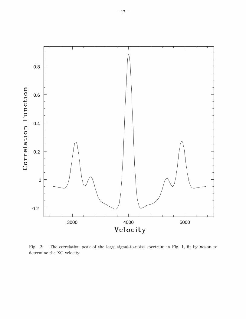
Figs. 6 – 8 explore these trends for a range of ∆V . The model velocity components haveflux ratios of 4:3, 2:1 or 4:1; the brighter component is always at the larger velocity. The modelspectra for each component are identical to the spectra above (e.g. Fig. 5b provides the pointswith ∆V = 160 km s−1 and flux ratio 4:1 for Figs. 6 – 8).

To explore the effects of lesser peaks on the derived velocity for the two techniques, wecompare XC and SEMLF results to the velocity of the brightest component. Fig. 6 shows thedifference between the velocity determined by each technique and the input model velocity of thebrighter component, as a function of ∆V . We compare the results to the flux-weighted mean ofthe Hα peaks (thin dotted line). The solid line shows the XC results; the dashed line shows theSEMLF results. For small ∆V , the XC line is close to or above the SEMLF line — the XC velocityis generally closer to the velocity of the brighter component and SEMLF tracks the flux-weightedmean. At larger ∆V , in models with larger component flux ratios, the lines cross — SEMLFstops tracking the flux-weighted mean and the SEMLF result is closer to the velocity of the brightcomponent. In the 4:3 flux ratio model, SEMLF switches to fitting only the brighter peak at∆V ≥ 280 km s−1 (not shown); in this model, the greatest difference between the velocities fromthe two techniques is 44 % of the component separation, when ∆V = 240 km s−1 = 2.3 times theFWHM of Hα. In summary, at low component separation, for all the models, SEMLF fits closerto the mean of the components, while XC fits closer to the brightest peak. At larger componentseparation, when the component flux ratio is large, this trend reverses and SEMLF fits the brighter

– 9 –

peak only.

Fig. 7 shows the errors computed by each technique as a function of component velocityseparation, for XC (solid line) and SEMLF (dashed line — unweighted; dotted line — weightedby χ2). These figures illustrate the necessity of weighting the formal SEMLF errors by χ2. TheXC errors and the weighted SEMLF errors increase dramatically as ∆V increases, indicating thepresence of additional components, although the weighted SEMLF errors begin to decrease againat very large ∆V , for 2:1 or 4:1 flux ratios, when only the strongest peaks enter the fit. In thiscase, the χ2 remains large, as shown in the next figure.

In Fig. 8a and b, we illustrate the behavior of the XC errors and of the χ2 of the SEMLFGaussian fits for flux ratios of 4:3 and 4:1; we plot the r value on top, then ω, then χ2. In the 4:1flux ratio model ω increases until ∆V is so large that only one component contributes to the fitand ω begins to decrease. However, r decreases with ∆V for each model at large ∆V , signalingthe increasing inadequacy of a single-component template as the velocity components separate.The decrease in r accounts for the increase in the errors; thus the errors increase monotonicallyas ∆V increases. Likewise, χ2 increases rapidly as ∆V increases, slowing only at the very largest∆V , where the component ratio is 4:1.

In these examples, XC and SEMLF compute velocities which differ by up to 44 % of thecomponent velocity separation. XC errors increase monotonically, and by a large factor, as thevelocity component separation (∆V ) increases. For larger component flux ratios, the unweightedSEMLF errors remain small and begin to decrease at large ∆V , making them unsuitable forspectra with multiple velocity components. The χ2 – weighted SEMLF errors behave much morelike the XC errors, increasing by large factors as ∆V increases, although they do not increasemonotonically for large component flux ratios with large ∆V . Note that because the χ2 takenalone does increase monotonically, χ2 is preferable to the weighted error as an indicator of multiplevelocity components when using SEMLF.

The cross-correlation technique flags the multiple-component case consistently, even as thesecondary component becomes weak or widely separated in velocity from the primary component.Cross-correlation errors are less model-dependent than formal χ2-minimization errors in the sensethat they include mismatch between the model (the template) and the spectrum. Thus in spiteof a template-dependent systematic bias in the errors, the cross-correlation errors roughly scaleproperly; they even reflect velocity components that do not overlap the strongest componentin wavelength. The χ2 of the SEMLF technique also reflects the presence of secondary velocitycomponents that overlap the main component in wavelength.

4. Two-Dimensional Model Rotation Curves

Here, we model effects from multiple velocity components that can be important in longslitgalaxy spectroscopy. We compare the results of XC and SEMLF.

– 10 –

4.1. Non-Gaussian Profiles

When neighboring discrete disk components of a galaxy are not sufficiently resolved, theyoverlap spatially, resulting in spectra with multiple velocity components. Spectra with multiplevelocity components also occur when galaxies have kinematically distinct, cospatial components,like circumnuclear disks. We illustrate these two cases with two-dimensional models of “rotationcurves”; we construct the models using artificial one-dimensional emission-line templates, orsums of templates, created with linespec in RVSAO, joined with mk1dspec and mk2dspec inNRAO.ARTDATA.

Fig. 9 is an image of a model spectrum which illustrates spatially overlapping components.Fig. 9a shows a greyscale plot of the region around Hα of the model longslit spectrum —the dispersion axis is horizontal, while the spatial axis is vertical and spans 100 pixels. Ourtwo-dimensional spectra consist of segments (the lumps in the image) with Gaussian intensityvariations in the spatial direction. The horizontal lines in the top portion of Fig. 9b show eachsegment as a horizontal line across its spatial FWHM, where the spatial direction is along thex-axis. The actual “emission” extends beyond its FWHM. The y-axis shows the velocity of eachsegment. The circles show the results from XC (left) and SEMLF (right), with the errors on anexpanded scale at the bottom of the figure. We show both unweighted SEMLF errors and SEMLFerrors weighted by χ2.

The velocity structure is Gaussian and does not vary along each segment; line profiles areirregular (e.g. double-peaked) where the segments overlap and thus more than one segmentcontributes to the spectrum. Widths in the dispersion direction are fixed by the basic spectrum,Fig. 1, used in the models. As in the one dimensional case, we add read noise (7.0 e−) and Poissonnoise to the spectra using mknoise in NRAO.ARTDATA. Although the model is a step function invelocity, the calculated rotation curve varies smoothly because the segments at different velocitiesoverlap spatially.

The biggest differences between the XC and SEMLF curves occur between segments, at pixel∼55. The errors behave similarly for the two techniques. The errors for both models increasesignificantly in the overlap regions; they are larger where adjacent components are separated bylarger velocities. The weighted SEMLF errors increase by a larger factor than the unweightederrors increase. As expected, ω increases in the regions of overlap, and r decreases; r also decreaseswhen the signal fades (e.g. at pixel values > 95).

The model in Fig. 10a resembles a 2-component galaxy with an inner disk (see e.g. Rubin etal. 1997). Fig. 10b shows the positions and velocities of the segments; each segment has a FWHMof 4 pixels in the spatial direction, although we plot only points. The outer disk model (dashedline) approximately traces a standard rotation curve. The second model component (thick solidline) represents an inner gas disk; it rotates as a solid body, is twice as intense as the outer curve,and has emission lines twice as broad.

– 11 –

Fig. 10b shows that the techniques fit similar rotation curves, with similar errors, to themodel. In the cross-correlation case, the 1

1+r contribution to the error decreases in the centerof the model due to larger signal, but the cross-correlation errors increase because ω increases,signaling the presence of the second, distinct velocity component (see Fig. 10b).

When the formal SEMLF errors are not weighted by χ2, the errors decrease in the center ofthe model due to the larger S/N ratio. Only χ2–weighted errors reflect the velocity uncertaintydue to the two components, because χ2 increases as a single Gaussian becomes a poor fit.

4.2. Nonstandard Line Ratios with Non-Gaussian Profiles

Nonstandard line ratios (e.g. in the nuclear regions of AGN) are another potential source oftemplate or model mismatch. In real galaxies, non-thermal activity and multiple components oftenarise together; we consider a combined model here. We compare the XC and SEMLF responsesto nonstandard line ratios in the nuclear region using the “inner disk” model; we plot results inFig. 11. The left column of Fig. 11 shows the model of Fig. 10 on top, the XC velocity minus theSEMLF velocity in the middle, and the errors from the two techniques on the bottom. The middlecolumn model has [NII] lines with heights greater by a factor of ten in the inner disk component;the outer disk and the [SII] and Hα lines remain the same. The model we show in the right columnhas [NII] lines that are ten times larger and no Hα emission in the inner disk component. Again,the outer disk and [SII] profiles remain the same — thus, there is a small amount of Hα emissionfrom the outer disk component. The velocity structure of the models remains the same.

The changing line ratios influence the results of the techniques somewhat, especially at theedge of the inner disk component. The peak difference between SEMLF and XC results occurs ataperture 40 in Fig. 11e, where the difference is 60 km s−1, corresponding to 52% of the velocitydifference between the inner and outer disks at that aperture. In XC, the contributions to thevelocity from each emission line are effectively weighted by their heights in the template. Hα is thestrongest emission line in the HII region template we use. Thus, XC weights the contribution ofthe faint outer disk much more heavily than SEMLF does, due to its small amount of Hα emission.Peak heights in SEMLF may vary to accommodate changing line ratios; thus the SEMLF errorsincrease only moderately. The XC errors increase due to spectrum/template mismatch. Whenthe mismatch is severe, the templates can be adjusted. For example, when Balmer absorptioneliminates Hα, the line can be removed from the template.

Increased errors may result from many sources, including changing line ratios, lower S/N,or additional velocity components. All three of these effects increase the r error statistic in XC.ω reflects multiple velocity components that are not spaced too widely. To determine the causeof increased errors, it is usually necessary to examine the line profiles in the region of interest.However, the dip in the computed rotation curve at the transition between the inner and outerdisk (Fig. 10, aperture 43), accompanied by the increased error, or especially by an increased ω,

– 12 –

provides a strong clue to the nature of the increase — a second velocity component. In automatedreduction with XC, one can select out rotation curves where there are many adjacent points withlarge errors as candidates for multiple-component systems. With SEMLF, the formal errors donot clearly reflect additional components; they flag only regions of low S/N ratio. The effects ofspectrum/model mismatch are isolated by χ2; regions with multiple velocity components can beflagged as regions where χ2 is significantly greater than 1.

5. Application of XC to Real Galaxies

Barton et al. (1999) use XC to reduce a large sample of rotation curves of galaxies in pairs;Fig. 12a shows an example. Barton et al. (1999) describe the reduction procedures in detail. Thecurve shows the inner part of CGCG 373-046, which has a separate kinematic component in thecenter. The errors enlarge in the center to reflect this component. Fig. 12b shows Hα and [NII]line profiles at various slit positions; the line profiles are clearly doubled near the center of thegalaxy, where the errors enlarge.

The models described in this paper explore only the simplest cases; they exclude the effectsof uncertainty in wavelength solution, night sky contamination, cosmic rays, non-Gaussian lineprofiles other than multiple-component profiles, continuum emission and extra emission lines(that are not included in the template spectra). At minimum, the steps necessary for longslitredshift reduction are: (1) bias subtraction and flat-fielding, (2) “line-straightening,” or solvingfor the wavelength solution at each pixel in the spatial direction, (3) cosmic-ray removal and skysubtraction, (4) a correction for differential atmospheric refraction and (5) a redshift determinationat each point along the slit.

Template selection or construction is also necessary, after step (4), when cross-correlationis used in step (5). The best template will reflect the spectrum of a typical single-velocitycomponent. Barton et al. (1999) build cross-correlation templates using the observed relativeline heights and widths. To measure line heights and widths for the template, they run the taskemsao in the RVSAO package (Kurtz & Mink 1998) which fits unconstrained Gaussian functionsto the major emission lines with enough signal. They use each aperture in which emsao findsall 5 emission lines; they compute the median relative line heights and the median absolute linewidths for each run (4 – 5 nights). Barton et al. use the resulting values as input parameters tocreate a template of smooth Gaussian “emission” lines with linespec in RVSAO. They test theperformance of separate templates for each observing run, night, and galaxy and find that a runtemplate yields the smallest errors on average. In practice, a single, carefully constructed templateused for all data from a particular instrumental setup should suffice for most purposes (see Kurtz& Mink 1998).

For the low S/N case, a small amount of fine-tuning is necessary to extract complete rotationcurves; Barton et al. find that restricting the wavelength range of allowable solutions to within

– 13 –

∼1000 km s−1 of the systemic velocity is easy to implement and yields accurate curves in low S/Nregions, although it may exclude extreme cases of separate velocity components. For example,Morris et al. (1985) find a component of NGC 7582 1300 km s−1 off the systemic velocity. .

6. Conclusion

We describe the use of cross-correlation to determine velocity fields of nearby galaxies usingoptical emission lines observed with longslit spectroscopy. The method is easily automated, makessimultaneous use of the strongest emission lines, and is efficient for low signal-to-noise spectra. Aswe describe, the technique yields well-defined errors.

We compare cross-correlation to a fundamentally different, parametric technique, simultaneousGaussian fitting of emission lines. Velocities and errors computed by the two techniques agreevery well in the case of a single Gaussian velocity component.

When line profiles are non-Gaussian (e.g. because more than one component contributes atthe same slit position), the results of the two techniques differ. In our examples, the XC andSEMLF techniques give velocities which differ by up to 52 % of the component velocity separation.For standard HII region emission line ratios and component separations up to 1.5 times theFWHM of Hα, XC fits closer to the brightest peak and SEMLF fits closer to the mean. As theseparation becomes larger, SEMLF also switches to the brightest peak.

The formal SEMLF error and the error computed by XC differ significantly because theXC error consistently reflects mismatch of the spectrum and model (template), whereas formalSEMLF errors are model-dependent. However, when SEMLF errors are weighted by χ2, SEMLFerrors behave much more like XC errors. Only minor differences remain, as the SEMLF errorsdo not increase monotonically in reflecting components with increasing velocity separation fromthe primary velocity component. Thus, the χ2-weighting procedure is empirically justified bycomparison with XC.

For automated reduction of large data sets, multiple components and other non-Gaussianline structures can be flagged for further inspection using the increase in either the XC error (orthe statistic ω), or the SEMLF χ2. However, a complete description of these multiple-componentcases requires additional modeling to explore the different components.

The choice of whether to use XC or SEMLF should be guided by the following considerations:(1) XC is readily available as the IRAF routine xcsao, in the RVSAO package. It is easilyautomated and requires no initial redshift guess (although constraints on the allowed solutions areuseful for spectra with small S/N ratios), (2) for two-component profiles, XC generally fits closerto the brighter peak, whereas SEMLF shifts from fitting the flux-weighted mean to fitting thebrighter peak for larve ∆V and large flux ratios, (3) both XC errors and the SEMLF χ2 statisticmay be used to flag multiple components, (4) the XC error increases monotonically with peak

– 14 –

velocity separation, as does the SEMLF χ2, but the SEMLF errors do not behave monotonicallybecause at large ∆V , SEMLF switches to fitting only the brightest peak, (5) SEMLF errors areexact in the ideal Gaussian case, whereas the overall normalization of the XC errors must becalibrated for each template if ±20% errors are not accurate enough, (6) in XC the choice oftemplate fixes the model emission line ratios and linewidths, whereas these can vary (or be fit), inSEMLF, and (7) SEMLF measures shape information for the line profiles in the single-Gaussiancase.

We thank D. Fabricant, D. Mink and S. Tokarz for useful discussions and assistance with thesoftware. E. B. and S. K. received support from Harvard Merit Fellowships. E. B. received supportfrom a National Science Foundation Graduate Research Fellowship, and S. K. received supportfrom a NASA Graduate Student Researchers Program Fellowship. This research was supported inpart by the Smithsonian Institution.

– 15 –

REFERENCES

Babcock, H. W. 1939, Lick Obs. Bull., no. 19, 41

Barton, E. J., et al. 1999, in preparation

Bureau, M., & Freeman, K. C. 1999, AJ, 118, 126

Burbidge, E. M., & Burbidge, G. R. 1975, in Stars and Stellar Systems, Vol. 4, Galaxies and theUniverse, ed. A. Sandage, M. Sandage, & J. Kristian (Chicago Univ. Chicago Press) 81

Courteau, S. 1997, AJ, 114, 2402

Franx, M., Illingworth, G., & Heckman, T. 1989, ApJ, 344, 613

Kannappan, S. J., et al. 1999, in preparation

Keel, W. C. 1996, ApJ, 106, 27

Kurtz, M. J., & Mink, D. J. 1998, PASP, 110, 934

Landsman, W. B. 1995, in Astronomical Data and Analysis Software and Systems IV, ASPConference Series, Vol. 77, R.A. Shaw, H.E. Payne, and J.JE. Hayes, eds., p. 437

Marziani, P., Keel, W. C., Dultzin-Hacyan, D., & Sulentic, J. W. 1994, ApJ, 435, 668

Mathewson, D. S., Ford, V. L., & Buchhorn, M. 1992, ApJS, 81, 413

Marquez, I., & Moles, M. 1996, A&A, 120, 1

Merrifield, M. R., & Kuijken, K. 1994, ApJ, 432, 575

Morris, S., Ward, M., Whittle, M., Wilson, A. S., & Taylor, K. 1985, MNRAS, 216, 193

Osterbrock, D. E. 1989, Astrophysics of Gaseous Nebulae and Active Galactic Nuclei (Mill Valley:University Science Books)

Pease, F. G. 1918, Proc. Natl. Acad. Sci., 4, 21

Press, W. H., Teukolsky, S. A., Vetterling, W. T., & Flannery, B. P. 1992, Numerical Recipes inC, Second Edition (Cambridge: Cambridge Univ. Press)

Rix, H.-W., & White, S. D. M. 1992, MNRAS, 254, 389

Rubin, V. C., Burstein, D., Ford, W. K., Jr., & Thonnard, N. 1985, ApJ, 289, 81

Rubin, V. C. 1995, ApJ, 451, 419

Rubin, V. C., Kenney, J. D. P., & Young, J. S. 1997, AJ, 113, 1250

Tody, D. 1986, in Proc. SPIE Instrumentation in Astronomy VI, ed. D. L. Crawford, 627, 733

Tody, D. 1993, in Astronomical Data Analysis Software and Systems II, A.S.P. Conference Series,Vol. 52, eds. R. J. Hanisch, R. J. V. Brissenden, and J. Barnes, 173

Tonry, J. L., & Davis, M. 1979, AJ, 43, 393 (TD)

van der Marel, R. P., & Franx, M. 1993, ApJ, 407, 525

This preprint was prepared with the AAS LATEX macros v4.0.

– 16 –

6600 6700 6800 6900

0

200

400

600

Fig. 1.— The basic model spectrum, shifted to 4000 km s−1.

– 17 –

3000 4000 5000

-0.2

0

0.2

0.4

0.6

0.8

Fig. 2.— The correlation peak of the large signal-to-noise spectrum in Fig. 1, fit by xcsao todetermine the XC velocity.

– 18 –

-40 -20 0 20 40

0

50

100

150

Fig. 3.— 283 Gaussian spectra at different noise levels: (a) histogram of the difference between thetrue velocity and the XC velocity (solid line), and the true velocity and the SEMLF velocity (dottedline) in km/s and, (b) histogram of the difference between the true velocity and the XC velocitydivided by the XC error (solid line), or the true velocity and the SEMLF velocity divided by theχ2-weighted SEMLF error (dotted line). The thick dot-dashed line is a Gaussian distribution withσ = 1.

– 19 –

Fig. 4.— Two-component spectra with small and large component velocity separations, ∆V .The component flux ratio is 2:1. Each figure shows the spectrum (solid line) with SEMLF fit(dot-dashed line) and, XC (vertical dashed line) and SEMLF (vertical dotted line) results. (a)∆V = 60 km s−1 = 0.58 FWHMHα, where FWHMHα is the FWHM of the Hα line. The brightercomponent is at 4120 km s−1. The XC and SEMLF results overlap; they are 4101.2 ± 0.3 and4100.8 ± 0.3(±0.5) km/s, respectively, where the second SEMLF error is weighted by χ2. (b)∆V = 160 km s−1 = 1.5 FWHMHα. The brighter component is at 4720 km s−1; the XC andSEMLF results are 4701.3 ± 4.6 and 4672.8 ± 0.7(±10.9) km/s.

– 20 –

Fig. 5.— Two-component spectra. The component flux ratio is 4:1; the figure shows the spectrum(solid line) with the SEMLF fit (dot-dashed line) and, XC (vertical dashed line) and SEMLF(vertical dotted line) results. The component velocity separations are (a) ∆V = 60 km s−1 =0.58 FWHMHα, where FWHMHα is the standard deviation of the Hα line. The brightercomponent is at 4120 km s−1. The XC and SEMLF results overlap; they are 4109.6 ± 0.3 and4109.3 ± 0.3(±0.5) km/s respectively, where the second SEMLF error is weighted by χ2, and (b)∆V = 160 km s−1 = 1.5FWHMHα. The brighter component is at 4720 km s−1; the XC and SEMLFresults are 4714.0 ± 1.8 and 4715.0 ± 0.4(±3.0) km/s.

– 21 –

-60

-40

-20

-60

-40

-20

0 50 100 150 200

-60

-40

-20

Fig. 6.— Velocity offsets as a function of velocity component separation from two-componentspectra for XC (solid line) and SEMLF (dashed line). The velocity offset is equal to the velocitysolution minus the true velocity of brightest component in the model. The thin dotted line is theflux-weighted mean of the two components. The flux ratios are 4:3 (top), 2:1 (middle), and 4:1(bottom). For different spectral resolutions, ∆V must be scaled by 104 km s−1/FWHM, whereFWHM is for the the Hα line.

– 22 –

0

5

10

0

5

10

0 50 100 150 200

0

5

10

Fig. 7.— Velocity errors as a function of velocity component separation for XC (solid line) andSEMLF (dashed line). As in Fig. 6, the flux ratios are 4:3 (top), 2:1 (middle), and 4:1 (bottom).

– 23 –

0

50

100

150

200

200

300

400

50

100

150

140

145

Fig. 8.— Error contributions: r, ω and χ2 as a function of velocity component separation, ∆V ,for (a) the 4:3 flux ratio and (b) the 4:1 flux ratio. We omit the 2:1 flux ratio case, which looksqualitatively similar to (b).

4000

4200

4400

0 20 40 60 80 100

-10

0

10

20 40 60 80

Fig. 9.— “Overlapping segment” spectral model: (a) greyscale image, showing the model Hα andNitrogen lines; the dispersion axis is in the vertical direction and the spatial axis is horizontaland, (b) results and errors for XC and SEMLF. The top portion of (b) shows the rotation curvessuperimposed on the model flux components (solid horizontal lines), and the bottom portion showsthe error bars on an enlarged scale, including both weighted and unweighted SEMLF errors. Theleft sides of the rotation curves in (b) corresponds to the bottom of (a).

– 24 –

4000

4200

4400

0 20 40 60 80 100

-5

0

5

20 40 60 80

Fig. 10.— “Inner disk” spectral model (see Fig. 9 for a description of the figure, but note thedifferent error scale here). Note that the XC and weighted SEMLF errors increase in the center,reflecting the two kinematic components, but the (formal) unweighted SEMLF errors decrease inthe center — they fail to reflect the complex velocity structure.

– 25 –

4000

4200

4400

-60

-40

-20

0

20

40

60

40 50 60-60

-40

-20

0

20

40

Fig. 11.— XC and SEMLF velocity differences and errors for the “inner disk” model and modelswith varying line ratios for the inner disk component. The top figures are the XC rotation curves.The middle figures are the SEMLF velocity minus the XC velocity; the bottom figures are errorsfor each technique. (a) and (b) are the “inner disk” model from Fig. 10. (c) and (d) are the samemodel, except the [NII] line heights are increased by a factor of 10 for the wide inner disk velocitycomponent. (e) and (f) also have [NII] heights increased by a factor of 10, and no Hα emissionfrom the inner disk component.

– 26 –

3900

4000

4100

4200

110 120 130 140 150 160

-10

-5

0

5

10

6630 6640 6650 6660 6670 6680

130

135

140

Fig. 12.— The inner rotation curve of a real galaxy with a separate kinematic component in itscenter: (a) XC rotation curve and errors, and (b) Nitrogen and Hα line profiles at spatial positionsnear the center of the galaxy. Each profile is normalized for display purposes — the true emissionlines have more flux in the center than on the outskirts. The labels on the y axis correspond to thevalues on the x axis of (a).