employment and wage -...
TRANSCRIPT

POLICY RESEARCH WORKING PAPER 1524
Employment and Wage Cuts in Mexico's tariff levelswere associated with a slight
Effects of Trade decline in employment in
Liberalization Mexico and with increases inaverage wages (perhaps
reflecting improved
The Case of Mexican Manufacturing productivity in the reformedindustries and a shift toward
the use of more skilled
Ana Revenga workers). The wages and
employment of skilled
production workers were
significantly more responsive
to changes in protection
levels than those of
nonproduction workers.
The World Bank
Latin America and the Caribbean
Country Department II
Country Operations Division 1
October 1995
POCY RESFARCH WORKING PAI'FR 1524
Summary findingsIn 1985, after decades of an import-substitution She finds that reductions in quota coverage and tariffindustrial strategy, Mexico initiated a radical levels are associated with moderate reductions in firm-liberalization of its external sector. Between 1985 and level employment. A 10-point reduction in tariff levels1988, import licensing requirements were scaled back to (between 1985 and 1990) is associated with a 2- to 3-a quarter of earlier levels, reference prices were removed, percent decline in employment in Mexico.and tariff rates on most products were substantially Changes in quota coverage appear to have noreduced. By 1989, Mexico was one of the most open discernible effect on wages, but reductions in tariff levelseconomies in the developing world. are associated with increases in average wages. This
Adjusting to trade liberalization required the seems to reflect improved productivity in the reformedreallocation of resources betweeni sectors and entailed industries, which may be related to a shift toward the use
substantial dislocation of workers. Revenga analyzes how of more skilled workers.
Mexico's trade liberalization (1985-87) affected There seems to have been a slight shift in the skill mixemployment and wages in industry, focusing on how it in favor of nonproduction workers. This was paralleled
affected average employment and earnings rather than by a sharper increase in the wage differential between
on the link between trade and relative wages. She skilled and unskilled workers. The wages and
examines the tradeoff between wage and employment employment of skilled production workers wereadjustment, identifies which labor groups benefited more significantly more responsive to changes in protection
from liberalization, and tries to associate changes in levels than those of nonproduction workers - perhapsemployment and wages directly with measures of change partly because production workers were more heavily
in trade protection, rather than link them to changes in concentrated in the industries in which protection levels
imports and exports (which is more common). were grearly reduced.
This paper - a product of the Country Operations Division 1, Latin America and the Caribbean, Country Department 11
- was prepared for the World Bank labor markets workshop held in July 1994. Copies of this paper are available free from
the World Bank, 1818 H Street NW, Washington, DC 20433. Please contact Ana Revenga, room H5-189, telephone 202-
458-5556, fax 202-477-3378, Internet address arevenga(c/worldbank.org. October 1995. (31 pages)
rhe Policy Research Working Paper Series disseminates the findings of work in progress to encourage the exchange of ideas about
developmlent issues. An obiec-tilve ol the series is to get the findings out qutckly, even rf the presentations are less than fully polished. Thse
papers carry the names of the authors and should be used and cited accordingly. The findings, interpretations, and conclusions are the
auithors' own and should not be attributed to the W'orld Bank, its Executive Board of Directors, or any of its memnber countries.
Pro(diuced by the Policy Research Disseminationi Center

EMPLOYMENT AND WAGE EFFECTS OF TRADE LIBERALIZATION:THE CASE OF MEXICAN MANUFACTURING
Ana Revenga
I am grateful to Ann Harrison and Jim Tybout for their invaluable help in obtaining the data,and to Linda Bell, David Card, Susan Collins, Richard Freeman, Elizabeth King, and AnnHarrison for providing very helpful comments. Useful suggestions from participants at the July1994, World Bank Labor Markets Workshop are also gratefully acknowleged.

/

I. Introduction
In 1985, after decades of pursuing an import-substitution industrialization strategy,
Mexico initiated a radical liberalization of its external sector. The scope and speed of this trade
liberalization episode is apparent from Table 1.1 Between 1985 and 1988, import licensing
requirements were scaled back to about a quarter of their previous levels, reference prices
were removed and tariff rates on most products substantially reduced. By 1989, Mexico was
one of the most open economies in the developing world.
Adjusting to this episode of trade liberalization required a substantial reallocation of
resources between sectors of the Mexican economy. On the whole, the process was fairly
smooth and its costs in terms of aggregate unemployment quite moderate: Mexico's
unemployment rate rose to 4.4% in 1985, but was back down to 2.9% by 1989. One
explanation for the absence of large aggregate employment effects was the flexibility
demonstrated by real wages, which declined significantly throughout the adjustment period.
However, while on the aggregate the employment costs of the liberalization may have
been fairly small, there is no doubt that at the sectoral level there was substantial dislocation
of workers. Understanding how adjustment occurred at this level -- whether there was a
tradeoff between employment and wage responses, and how this may have varied across
sectors -- could provide essential insights as to the broader workings of the Mexican labor
market. This seems particularly relevant in the wake of the implementation of the North
American Free Trade Agreement (NAFTA), as further labor reallocation is expected.
Beyond its interest in relation to the potential effects of NAFTA, Mexico's recent trade
liberalization experience can be relevant to many other developing countries embarking on a
similar process. One of the key concerns regarding any liberalization episode is its potential
effects on employment and wages in the affected sectors. Understanding what the
employment costs were in the Mexican case, and how they may have been dampened, may
thus provide some useful lessons.
1 For a careful account of the Mexican trade liberalization experience see Ten Kate (1992).
2
With these general objectives in mind, this study analyzes the impact of the Mexican
trade liberalization of 1985-87 on employment and wages in the industrial sector. The paper
examines the tradeoff between wage and employment adjustment, and analyzes whether
certain groups of labor benefitted more, in relative terms, from the liberalization. The data used
for the analysis are plant-level data drawn from the Annual Industrial Survey, and cover a
panel of medium-to-large firms over the 1984-1990 period. These data were combined with
import penetration ratios at the sector level, and with tariff-line and license-coverage data.
This paper is part of a new wave of interest in the Mexican labor market. Motivated
partially by the U.S. literature on trade and rising inequality, a number of recent papers have
investigated the impact of trade on the Mexican wage structure. Results so far are are fairly
mixed: most coincide in finding a rising trend for wage inequality in Mexico, but differ widely
when it comes to its explanation. Feliciano (1994), for example, uses household-level data to
examine the effect of liberalization on the retums to schooling. She finds that wage
differentials between skilled and unskilled workers increased between 1986 and 1990 and
attributes this increase to trade reform. Craig and Epelbaum (1994) document a similar rise in
eamings dispersion during the late 1980s, but associate it instead to a rise in the demand for
educated workers resulting from the complementarity between skilled labor and investment in
capital. Finally , Hansen and Harrison (1994) use both plant-level data and data from the
Mexican Industrial Census to assess whether increased wage inequality in Mexico was linked
to trade liberalization. They find little evidence of Stolper-Samuelson type effects, and
conclude that changes in Mexico's wage structure are driven mostly by developments within
industries.
This paper adds to the recent literature in several key aspects. First, it pays more
explicit attention to employment developments. Second, unlike the other papers, it focuses on
the impact of trade liberalization on average employment and earnings, rather than on the link
between trade and relative wages. Third, it attempts to associate changes in employment and
wages directly to measures of changes in trade protection, instead of linking them to changes
in imports and exports, as has been more common.
3

The rest of the paper is organized as follows. Section 11 lays down the main model to
be used as framework for the empirical analysis. Section III presents the data and some basic
descriptive statistics. Section IV shows the main econometric results. Section V examines
what has happened to skilled-unskilled wage differentials in response to trade liberalization.
Finally, Section VI concludes.
II. Estimating the Impact of Trade on Employment and Wages
This section outlines a simple model in which nominal wages are predetermined by
negotiation at the firm level, and employment is then set unilaterally by the firm after aggregate
prices and demand levels are known. I begin by developing the analysis of employment
determination, and then move on to consider how wages are set. This yields some simple
reduced-form equations for employment and wages. I then consider how these equations may
be extended to incorporate the effects of trade.
EmDlovment
Assume that there are i identical firms in each industry, and that each has a constant
returns to scale technology of the form:
(1) Yi,- ki = a[ni,-ki,I]+ Ei+
where yf is the output of firm i in period t, ki equals the capital stock of firm i in period t, nR
equals the firm's employment in that period, and en is a productivity shock which is assumed to
be serially uncorrelated. Note that all variables are expressed in terms of logarithms and that
industry subscripts are ommitted for simplicity.
Assume also that firms produce differentiated products, and that, therefore, they face
downward-sloping demand curves for their good. Let demand be allocated across firms as a
function of relative prices:
d d(2) Y -_Y = -_[P - Pt]
4

where yd represents demand for firm i's product in perod t, ytd is total industry demand in
period t, pH is the firm-specific price, pt is the average industry price, and ?I equals the price
elasticity of demand.
Profit-maximizing firms will find it optimal to set prices as a markup over marginal cost:
(3) Pj, =-In(@) +mci, withS = l -
and where
(4) mctt = Wit + (1 [yi kit] _n(a)a a
Combining equations (2), (3) and (4) yields the following price equation:
(5) p =-In(aO)+wit+ (- a), (p,tPt)+yd -kJ - aa a
Equation (5) can then be combined with equation (1) to obtain an expression for firm-level
employment:
(6)flit c + (2 - 1) kit - 77A(wz -pt) + Iy -(2-
awhere c = 2771n(a0)
a + iff]- a)
/
Waae Determination
Assume that wage setting is decentralized, and that as in many standard union models,
wage bargainers want to maximize the expected income of the representative worker. The
union, thus, sets real wages so as to maximize an objective function of the type:
5

(7) max V = ;r(w) * w + (1- r(w)) * wA
subject to employment being on the labor demand curve. Note that nr(w) equals the probability
that the representative worker will be employed in firm i the following period (which is a
decreasing function of the negotiated wage), and wA represents the "fall-back" or altemative
real wage (ie. the wage the worker will receive if he/she gets laid off).
If we assume that the union's target employment level is simply the employment level in
the previous period, nit-,, we can write the objective function as:2
(8) max nit (Wit) . nit-, - nit (Wit) nit-, nit-,
The standard solution to this type of bargaining model is of the form:3
(9) <( it -W = (nit - nit-l)
where G is the wage elasticity of labor demand. Adding and subtracting kit to the right-hand
side, and then substituting in from equation (6) for (nit - kit) gives us an expression for the
negotiated wage:
/
2 We are assuming that the union cares only about the interests of workers who are currently employed (ie. itsobjective is to maintain employment at current levels). This is consistent with the popular "insider-outsider' type ofmodels which have been developed to explain the persistence of European unemployment (see, for example,Lindbeck and Snower (1988); Layard, Nickell and Jackman (1991), Dolado and Bentolila (1992)).
3 See, for example, Layard, Nickell and Jackman (1991), De Lamo and Dolado (1991) or Dolado and Bentolila(1992).
6

(10) ~~~~~~~ +Ard (A2- J)ayWit = Cr + cw,t + icy-lt -ani--( )a ki, + 6
it
witha = _ _
(4+ 77A)
We now have an expression for firm-level employment (eq. 6) and firm-level wages (eq.10). The next step is to introduce tariffs and quotas into our framework, so as to obtainexpressions that allow us to relate employment and wages to trade liberalization measures.
Introducina Licensina and TariffsThe two key elements of Mexican trade policy prior to the liberalization were a system
of quantitative restrictions encompassing both quotas and licenses, and an ad valorem importtariff scheme .4 We consider the modeling of each in tum.
In analyzing the impact of QRs we distinguish between licensing of importedintermediate inputs, and that of final output. As regards the former, we can model thereduction of import restrictions as the release of a binding constraint on one factor, in our casek,. Using equations (1), (3) and (4) we have:
(11) Y, = ki+ [pi, - Wit]
where denotes the constrained factor. It is then clear that a reduction in licensing ofintermediate inputs should increase output and, to the extent that labor and the constrainedinput are complements in the production process, should also lead to an increase in theamount of labor employed.
'4 These two instruments were complemented by a set of official minimum prices for custom valuation. However,in this paper we ignore the role of these reference prices. For a description of the Mexican trade policies and theirevolution through the 1980s, see Ten Kate (1992).
7

We then tum to the impact of import licensing on final output. Assume that domestic
and foreign goods are imperfect substitutes, so that demand is a function of relative prices.
And let 8 represent the coverage of the quantitative import restrictions. We can then express
the fraction of total domestic demand for an industry's good that is allocated to domestic
producers in terms of relative prices and the coverage of the import restrictions. Letting lower
case letters denote logaritms,we have:
(12) Yt dt = In(J-S)+ O[, - p,]
where ddt reflects total domestic demand for the industry's good, (1-8) is the fraction of total
demand not covered by restrictions, and -p is the price of the import good which, in tum, is
assumed to be given by:
(13) p,=p (I+ tariff)
with p equal to the world price of the import good.
Making use of equations (11) through (13), we can rewrite our employment and wage
equations (6) and (10) as:
(14)n.k =a0 +a (r. -p p,)-a(w 1 -p)+a(vtp)nit = aO +l(it ~ it ) 2 (it -Pt ) 3 (vit -Pd )
b, [dd + ln(I - lcqj1 ) + 91n(1 + tariff. ) + 6(p - )]+ c ln(lci,t) +6 it
with a1+a2+a3=0, and
(15) wit = aoa + CUwit + a, a(rit -pt) + a3 a(vit - pt) +
bi a[dd, + In(l - Icq,t) + OIn(J + tariff i,) + O(pt - pt)] - a nizt- + cl a ln(lci2t) + vit
8
where (ra-pt) is the user cost of capital, (vit-p,) is the real price of materials, lcqft reflects thecoverage of quotas or licenses on output, and lcit reflects the coverage of licenses on inputs.
Equations (14) and (15) can be estimated jointly using Generalized Least Squares
(GLS).
Ill. Data Description and Basic Statistics
The data used in the empirical analysis are drawn from the plant-level Annual
Manufacturing Survey. The sample covers the period 1984-1990 and includes, within each
sector, all plants sorted by decreasing order of size to account for roughly 80% of cumulative
value added. Out of the 3218 plants included in the original survey, 2354 were selected forthe analysis.5 A very similar dat set has been used to study the impact of the liberalization on
productivity and performance, by Tybout and Westbrook (1992), and by Grether (1993). The
latter provides, in an appendix, a detailed description of the variables included in the survey
and of their construction.8
The plant-level data were combined with measures on tariff rates, and license coverage
on inputs and output calculated by the Mexican Trade Ministry (SECOFI), and with import
penetration ratios at the 3-digit sector level.7 Since the survey data do not include price
variables, these were taken from more aggregated sources. Producer-prices were obtained atthe 4-digit Mexican sectoral classification level and merged with the firm data. An aggregatewholesale price index, and a price index for raw materials were also added. Finally, we
5 Observations dropped included: (a) those with zero or negative values for gross output, value added and totalcosts; (b) those presenting large, erratic changes from year to year in the key variables; and (c) those with extremevalues for some of the essential variables relative to other plants in the same sector.
a One important characteristic of the sample is that it is closed -ie. only plants with observations for every yearof the sample period are included. This could introduce a potentially important selectivity bias into our analysis,since neither firms entering or exiting a sector during this period would be captured in the sample. Unfortunately, Iwas not able to obtain the complete unbalanced panel.
7 Import penetration ratios at the 3-digit ISIC level were available for 1984-87. Similar ratios at the 2-digit levelwere available for the complete sample period, 1984-90.
9

incorporated two altemative measures for the "fallback" wage. One is the average wage in the
state, which was drawn from the Industrial Census for several years. The other one is the
official minimum wage.
Means and standard deviations of the key variables are presented in Table 2. These
averages confirm that the sample comprises primarily large plants, although there is clearly
substantial variation both between and within industries. It is interesting that, despite the trade
liberalization measures, the mean import penetration ratio actually declined between 1984 and
1987. This reflects the fact that the impact of the liberalization was intentionally delayed by a
sharp 27% real depreciation of the peso in 1985 and 1986 (see Ten Kate, 1992). By 1987,
however, the depreciation had been reversed and the impact of the trade reforms began to
bite. Between 1987 and 1990, the mean import penetration ratio practically doubled,
increasing from 8.7% to 16.2%.
Table 3 presents means and standard deviations for log changes in the key variables
over the 1984-1986 and 1986-1990 periods. The table subdivides the sample into three groups
of industries according to their initial protection levels, and presents separate statistics for each
subgroup. To define the three industry categories, I first ranked industries by initial protection
levels (tariffs plus quotas): the top third was classified as high initial protection industries
(roughly those with quotas close to 100 percent of production and tariffs of above 40 percent);
the second third as medium initial protection (quotas of above 80 percent and tariffs of
between 20 and 40 percent); and the bottom third as low initial protection (for details on each
3-digit industry see Table 5).
The two phases of the liberalization process are clearly apparent from Table 3. During
the first phase, 1985-86, import quotas were removed and substituted for tariff-equivalents.
Accordingly, there were small overall reductions in average tariffs (of approximately -1.3
percentage points) but large decreases in quota coverage (on average of -67.2 percent). In
the second phase, tariff levels were brought down and remaining quotas removed. The largest
overall declines in protection rates occurred in those sectors which had previously been less
exposed to import competition. However, the pattern of liberalization differed somewhat
between industries: those classified as initially highly protected faced significantly smaller
declines in quota coverage during the first round of reforms and larger ones during the second
10

round than did the other sectors. Tariff reductions, on the other hand, were larger for the
initially protected sectors throughout the whole period.
Between 1984 and 1986, real output fell significantly in all industries, as did real wages.
The evolution of employment was somewhat more mixed: some sectors experienced stagnant
employment or even employment reductions, while others saw their employment levels grow.
Output recovered following the reforms, growing on average by nearly 4 percent. However,
sector performance diverged considerably, with the initially more-open industries showing
stronger growth. For the period as a whole (1984-90), industries classified as initially more
protected experienced lower employment growth over the period (measured both in terms of
workers and total hours), as well as sharper real wage declines.
The statistics presented in Table 3 suggest that both the magnitude of trade reform and
its impact have differed significantly across industries, with the initially highly protected sectors
bearing the largest adjustment burden. In order to understand how trade reform may have
played itself out through the Mexican labor market, the next step is to examine the
characteristics of the more affected sectors. Table 4 ranks 3-digit industries by descending
level of protection, and presents some basic statistics by industry.
Several features stand out from this table. First, industries with high initial protection
levels tended to be lower wage and more labor intensive than those with less protection.8
Sectors such as ceramics, apparel, footwear and furniture, for example, were among the most
protected, while industries like chemicals, steel and non-electrical machinery were relatively
more open. The rank correlation between total levels of initial protection and real wages is -
0.52 (significant at the .05 level), confirming that sectors with relatively low wages initially had
higher tariff rates and import quotas. Second, import penetration was significantly lower in
highly-protected, labor-intensive industries than in more open, capital-intensive sectors. In
1984, import penetration rates in ceramics, apparel and footwear were all under 3 percent. In
contrast, imports accounted for 20 percent of total consumption (output plus imports) in
chemicals, 31 percent in non-electrical machinery, and as much as 60 percent in electrical
machinery. Third, relative prices have fallen more in those sectors that experienced larger
8 This is consistent with Feliciano's findings that workers in highly protected industries had lower education andskills, and were paid less than those in less protected sectors.
11
trade reform: the rank correlation between changes in relative prices and changes in tariff
levels is -0.57 (significant at the .01 level), and the correlation between changes in relative
prices and changes in total protection (including removal of quotas) is -0.46 (significant at the
.05 level). Import shares have also increased slightly more in the large reform industries: on
average, import shares rose by 4 percentage points among the high reform industries and by 3
percentage points among the low reform ones. Import penetration in apparel, for example,
increased from 2.9 percent in 1984 to 8.6 percent in 1990. Similariy, import shares increased
from 5.3 percent to 11.4 percent in glass products, from 1.9 percent to 9.7 percent in textiles
and from 1.6 percent to 5.1 percent in footwear.
These overall patterns suggest a link between reduction in protection rates, increased
import competition, and employment and wage adjustment. This is supported by the
correlations presented in Table 5, which show a negative, although weak, correlation between
changes in import shares and changes in employment for the post-reform period. The data
show a similarly weak, negative correlation between changes in import penetration and output,
but a positive correlation between the former and real wages. The next section explores
these associations further in the econometric analysis.
IV. Results
The empirical results are based on the estimation of equations (14) and (15) described
above. The dependent variable in equation (14) is annual employment, measured both in
terms of average workers over the year and total hours worked. The independent variables
include the user cost of capital, the price of raw materials, the real hourly product wage,9 and
the protection rate variables: (a) the fraction of demand not covered by import restrictions (ie.
the inverse of the license coverage of output), (b) the average tariff rate at the end of the year,
and (c) the license coverage of inputs. All variables are expressed in logarithms, and all
nominal variables are deflated by the producer price index. To proxy for the evolution of total
demand for the industry's good, we have included industry-specific trends into our estimating
equations.10 We also include year effects to control for common aggregate shocks that are not
9 Because of potential measurement problems with the hours variable, I also tried using annual income ratherthan hourly wages as an independent variable. The results obtained were similar to those presented here.
10 In lieu of interactions between industry and year dummies.
12

otherwise captured by our specification. In addition, to allow for the possibility of slow
employment adjustment, we consider an altemative specification that includes lagged
employment among the right-hand side variables.
The bargaining model developed in section 11 would suggest that the appropriate wage
to use in equation (15) would be the real consumer wage --the nominal wage deflated by the
consumer price index. However, for consistency with the employment equation we have
opted for using the real product wage in this equation as well. The independent variables are
the alternative or "fallback" wage (defined as in section 1I1), employment lagged one period, the
user cost of capital, the price of raw materials, and the protection variables. As in the
employment equation, we include an industry-specific trend and year effects. We also allow for
a lagged dependent variable term. Again, all variables are expressed in logarithms.
Results are presented in Table 6. This table shows both simple unconstrained OLS
estimates obtained by estimating the employment and wage equations separately, and also
those obtained from estimating the two equations jointly by GLS. The OLS results foremployment levels are presented in columns (1) and (2), while those for hours are shown in
columns (3) and (4). OLS estimates for the hourly wage equation are presented in columns (5)
and (6). Joint estimates for the employment and wage equations are given in columns (7) and
(8), while joint estimates for the hours and wage equations are shown in columns (9) and (10).
Both sets of estimates --OLS and GLS-- are very similar.
As regards the employment equations, we obtain fairly reasonable estimates for factor
elasticities. The coefficient on the wage rate in the employment equation is negative and
significant, although as is often the case in employment demand equations it is very low. It is
significantly larger in the hours equation. Since we do not attempt to instrument for the real
wage in either case, these coefficients are probably downward biased. Although we do not
impose the constraint, the estimates are consistent with the restriction that the elasticities of
employment with respect to the three factor prices sum to zero.
With respect to the protection variables, our estimates are again quite reasonable. We
obtain a negative and significant coefficient on the variable that captures the fraction of
demand not covered by import restrictions. This suggests that an increase in the fraction of
13

the market not covered by restrictions (that is, a reduction in coverage levels) lowers
employment both in terms of workers and hours. Interestingly, the impact on number of
employees is quite similar to the impact on hours, suggesting little change in the amount of
hours worked per employee." Note that since all variables are entered in logarithms, the
coefficient must be interpreted as an elasticity.
The coefficient on tariff rates is, as we would expect, positive and significant. Hence, a
reduction in tariff rates is associated with a reduction in employment levels and total hours
worked. Again, the impact on both employment levels and hours worked are fairly similar.
Finally, with respect to licensing on inputs, we obtain a negative and significant estimate,
suggesting an effect that goes in the opposite direction from that of licensing on output: a
reduction of restrictions on imported inputs, appears to have a positive effect on employment.
My results for employment contrast strongly with those obtained by Feliciano (1994),
who does not find an impact of trade liberalization on industry-elevel employment. However,
Feliciano (1994) is analyzing total employment at the industry level, while I examine firm-level
employment.12 Oks (1993) has suggested that much of the improvement in productivity
following the reforms has occurred through within-industry changes in employment. Hence,
the effects of trade liberalization may not show up in net industry employment. Moreover,
Feliciano's employment regressions do not control for what happened to wages. If industries
experiencing large tariff reductions offered larger wage declines, the effects on employment
may have been dampened. Without controlling for wage developments, it may be hard to
isolate the impact of the changes in protection levels.
In both the worker and hours equations, the lagged dependent variable term appears
large and strongly significant. We interpret this as a sign of sluggish employment adjustment,
which is consistent with the existence of substantial employment protection. In any case, it
11 This finding contrast strongly with the experience of, for example, European countries, in which much ofadjustment to demand shocks appear to occur via changes in hours worked rather than via changes in employmentlevels. See Abraham and Houseman (1993).
12 Note also that Feliciano (1994) uses employment data from the National Accounts. These data may differsignificantly from those of the Manufacturing Survey because they reflect estimates of employment based on thenational account output data, rather than actual employment levels.
14

suggests that the dynamics of the equations are important. However, because of the limitedtime-period spanned by our sample, we have not experimented with longer lags.
The results for the wage equations are also quite satisfactory. The coefficients on boththe altemative wage and on lagged employment appear to be correctly signed and aresignificant. The results for the protection variables are a bit more mixed, but neverthelessreasonable. When the lagged real wage is ommitted from the specification, both the tariff rate
variable and the license coverage on imports come in as negative and significant. Thecoefficient on licensing of output, on the other hand, is insignificant. Although the results
weaken somewhat once a lagged dependent variable is included in the specification, the signs
remain the same.
The estimates suggest that a reduction in tariff rates is associated with an increase in
real wages. A priori, one may have expected the sign to go the other way, under the
assumption that workers appropriate part of the rents created through tariff protection.'3 But
this does not seem to be the case. This finding is reinforced by the zero coefficent on
licensing of output. If workers had been able to appropriate part of the rents created by the
existence of quotas, you would expect their removal to be associated with a decline in real
wages.
One interpretation of the finding that tariff reductions are associated with increased realwages is that it reflects an increase in labor productivity in response to the trade reforms.'4 A
complementary explanation is that the skill mix of employment may be changing. If lower skillor less senior workers were laid off in response to the reforms, tariff reductions would then beassociated with an increase in the average wage (and also with an increase in averageproductivity).
13 Revenga (1993) finds that in the U.S., increases in import competition are associated with small, butstatistically significant real wage declines, and that these declines are larger in highly unionized industries, in whichworkers had presumably been more able to appropriate rents.
14 Combined with the result on employment, this finding suggests that a reduction in tariffs is associated with a(simultaneous) reduction in employment levels and increase in wages.
15

As with tariffs, the reduction in the licensing of inputs appears to be linked to an
increase in real wages. Again, this could reflect an improvement in productivity, resulting from
the release of the input constraint that allows the firm to use more (imported) capital and/or
other intermediate inputs, or from a change in the skill mix of employment toward more skilled
workers.
To test whether the negative sign on the tariff variable is explained by productivity
increases, I estimate a version of equation (15) with value added per worker (as a proxy for
productivity) entered as a right-hand side variable. Because of the potential endogeneity of
the productivity variable, it is entered lagged one period. This equation can be interpreted as a
reduced-form for wages that takes into account productivity changes. Results are shown in
Table 7. As far as the employment and hours equations are concemed, adding value added
per worker to the equation does not greatly alter the estimated coefficients for the protection
variables. The results for the wage equation are somewhat more interesting, particularly those
in column (6), which includes the lagged real wage as a independent variable. As expected,
lagged value added per worker enters positively in the regression indicating a relationship
between higher productivity and higher real wages. The coefficient on the portion of domestic
demand not covered by quotas is negative and significant, suggesting that a reduction in
quotas (an increase in the fraction of the market not covered by restrictions), holding
productivity constant, reduces real wages. This is consistent with workers having appropriated
some part of the quota rents prior to liberalization. Note, however, that although significant the
coefficient is very small, not quite -0.01. The coefficient on tariffs remains negative, but
becomes insignificant once the lagged dependent variable is included in the regression. This
finding can be taken as weak evidence that the link between tariff reductions and wage
increases works through productivity.
V. Trade Liberalization and Skilled-Unskilled Wage Differentials
The finding that tariff reductions are associated with increases in average wages,
suggests that the skill composition of employment in Mexican manufacturing may be shifting
towards more-skilled or more-senior workers. This would be consistent with the increase in
skill differentials documented by Feliciano (1994), Craig and Epelbaum (1994) and Hansen
16
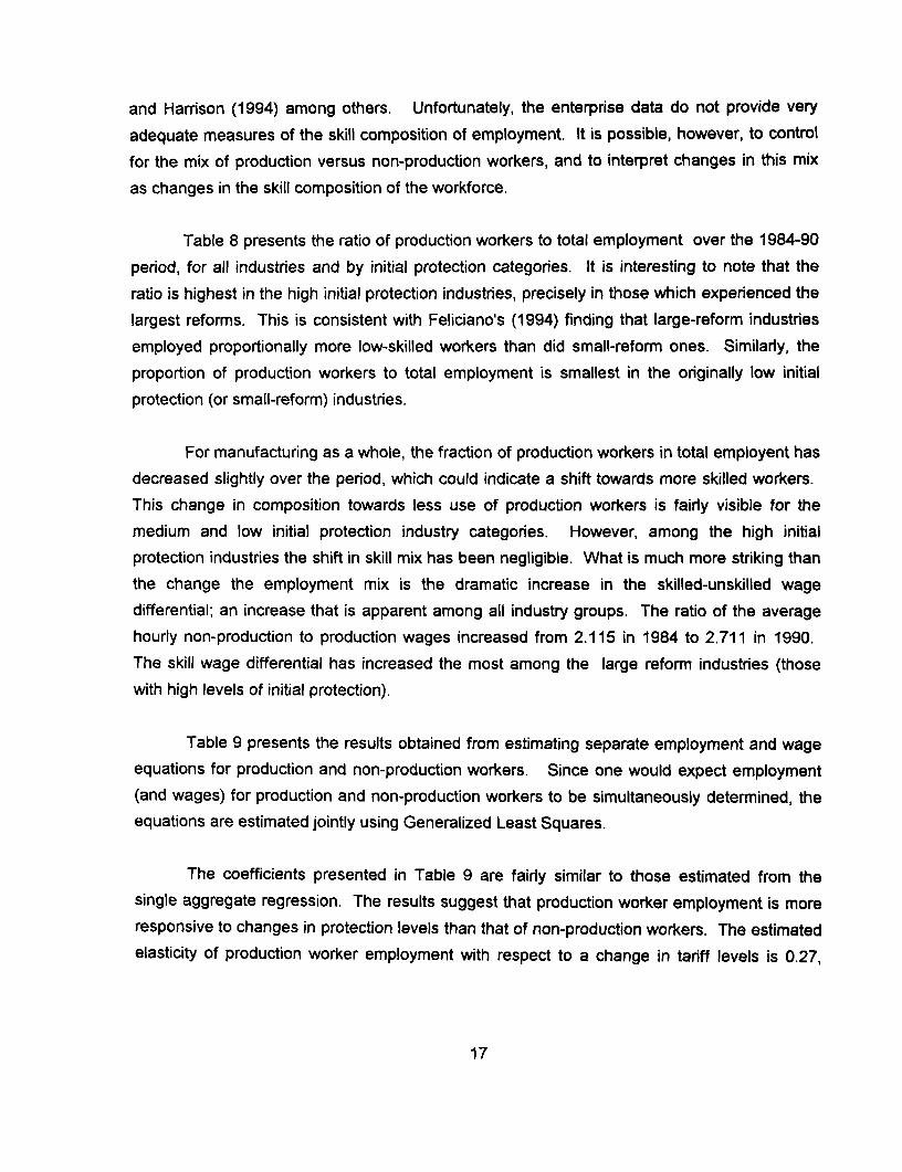
and Harrison (1994) among others. Unfortunately, the enterprise data do not provide very
adequate measures of the skill composition of employment. It is possible, however, to controlfor the mix of production versus non-production workers, and to interpret changes in this mixas changes in the skill composition of the workforce.
Table 8 presents the ratio of production workers to total employment over the 1984-90
period, for all industries and by initial protection categories. It is interesting to note that theratio is highest in the high initial protection industries, precisely in those which experienced thelargest reforms. This is consistent with Feliciano's (1994) finding that large-reform industries
employed proportionally more low-skilled workers than did small-reform ones. Similarly, the
proportion of production workers to total employment is smallest in the originally low initial
protection (or small-reform) industries.
For manufacturing as a whole, the fraction of production workers in total employent has
decreased slightly over the period, which could indicate a shift towards more skilled workers.
This change in composition towards less use of production workers is fairly visible for the
medium and low initial protection industry categories. However, among the high initial
protection industries the shift in skill mix has been negligible. What is much more striking than
the change the employment mix is the dramatic increase in the skilled-unskilled wage
differential; an increase that is apparent among all industry groups. The ratio of the average
hourly non-production to production wages increased from 2.115 in 1984 to 2.711 in 1990.
The skill wage differential has increased the most among the large reform industries (those
with high levels of initial protection).
Table 9 presents the results obtained from estimating separate employment and wage
equations for production and non-production workers. Since one would expect employment
(and wages) for production and non-production workers to be simultaneously determined, theequations are estimated jointly using Generalized Least Squares.
The coefficients presented in Table 9 are fairly similar to those estimated from thesingle aggregate regression. The results suggest that production worker employment is more
responsive to changes in protection levels than that of non-production workers. The estimated
elasticity of production worker employment with respect to a change in tariff levels is 0.27,
17

whereas that for non-production employment is 0.14. The results also suggest that the wage
elasticity of employment is larger for production workers than for non-production employees.
The wages of non-production workers do not appear to be very responsive to changes
in protection levels, whereas those of production workers do seem to respond. Reductions in
quota coverage of imported inputs are associated with increases in production worker wages,
perhaps reflecting increases in productivity resulting from greater access to imported capital
and/or other inputs. Reductions in tariff levels are, again, associated with higher wages,
suggesting that the production/non-production breakdown is not sufficient to control for
changes in the skill mix of employment.
The fact that production worker employment is more responsive to tariff changes than
non-production employment could possibly be explained by the fact that the former are more
highly concentrated in the those industries that experienced large declines in protection. To
explore this hypothesis, I examine what happened within industries. I run separate
employment and wage equations by industry category. I find that in all three industry
categories employment and wages of production workers are substantially more responsive to
changes in protection levels than those of non-production workers. I also find, however, bigger
responses among the industries that experienced greater reform (namely those with high or
medium levels of initial protection). Hence, the aggregate results appear to be driven both by
differences in responsiveness within industries (with production workers being more affected
by reform) and by cross-industry variation in the skill mix.
VI. Conclusions
This paper has analyzed the impact of trade liberalization on employment and wages in
Mexican manufacturing using a panel data set of firms for the 1984-90 period. The paper finds
that reductions in quota coverage and in tariff levels are associated with moderate reductions
in firm-level employment. According to the results of this paper, a 10 point reduction in tariff
levels, such as that experienced by Mexico between 1985 and 1990, is associated with a 2-3%
decline in employment. Changes in quota coverage appear to have no discernible effect on
wages. But reductions in tariff levels are associated with increases in average wages. This
18

last result seems to reflect productivity increases in the reformed industries, which may be
related to changes in the composition of labor towards higher-skilled workers.
The data suggest that there has been a slight shift in the skill mix in favor of non-
production workers. This has been paralled by a much sharper increase in the skilled-unskilled
wage differential. When equations are estimated separately for producton and non-
production workers, the paper finds that employment and wages of the former are significantly
more responsive to changes in protection levels than those of the latter. This should be
atributed, in part, to the fact that production workers are more heavily concentrated in the
industries that underwent large reductions in protection levels.
19

Table I
Mexico: Trade Protection in Manufacturing, 1985489
1985:Vl 1986:VI 1987:VI 1988:Vl 1989:VI 1990:VIl
Avg. Tariff' 23.5 24.0 22.7 11.0 12.6 12.5(% ad valorem)
Maximum Tariff 100.0 45.0 40.0 20.0 20.0 20.0
Coverage of Import 92.2 46.9 35.8 23.2 22.1 19.9Licensingb
Coverage of Reference 18.7 19.6 13.4 0.0 0.0 0.0Pricesb
* Production-weighted. Does not include the uniform 5% surcharge that was abolished in December, 1987.b Average share of output subject to import licensing or reference prices, as a percentage of total domestic output.
Source: Hufbauer and Schott (1992), Grether (1993).
20

Table 2
Sample of Mexican Manufacturing Firms, 198440
Means (s.d.) of Key Variables
1984 1987 1990
Total Employment 331.7 334.8 352.7(636.9) (637.1) (688.4)
Production Workers 231.7 231.9 245.3(489.0) (487.6) (529.2)
Non-production Workers 99.8 102.6 106.2(173.9) (179.8) (189.8)
Real Gross Value Outout 370.5 411.9 437.4(millions of 1980 MEX$) (888.9) (1117.8) (1257.0)
Real Value Added 156.1 171.3 182.9(millions of 1980 MEX$) (361.6) (428.1) (478.5)
Real Monthly Waqe 6981.4 6445.4 6835.4(1980 MEX$) (2942.6) (2920.5) (3548.7)
Production Workers 5461.2 4932.4 4701.4(2173.8) (1969.8) (2134.8)
Non-Production Workers 10,353.5 9652.0 11,502.6(6046.4) (4736.9) (6855.7)
Imoort Penetration Ratio (9) 12.7 8.7 16.2(2-digit) (16.1) (11.5) (15.2)
21

Table 3Long Period Changes:
Means of Log Changes by Initial Protection Levelt
1984-1986
Log Change in: All Low IP Medium IP High IP
Total Emplovment 0.016 0.026 0.007 0.009(0.389) (0.245) (0.215) (0.245)
Total Hours Worked 0.014 0.031 0.010 0.017(0.428) (0.295) (0.229) (0.287)
Real Gross Value Output -0.054 -0.042 -0.080 -0.042(0.377) (0.400) (0.347) (0.380)
Real Hourly Waae -0.053 -0.050 -0.064 -0.046b (0.247) (0.271) (0.207) (0.257)
Imoort Penetration Ratio 0.004 0.002 0.006 0.005(0.029) (0.042) (0.024) (0.011)
Averaae Tariffb -1.31 7.260 1.595 -13.583(15.1) (9.929) (6.869) (17.854)
Domestic Production covered -67.2 -71.785 -77.930 -51.315by Import Licenses" (37.2) (30.749) (27.673) (46.150)
1986-1990
Log Change in: All Low IP Medium IP High IP
Total Emplovment 0.008 0.019 0.027 0.001(0.521) (0.375) (0.361) (0.342)
Total Hours Worked 0.022 0.034 0.041 0.011(0.530) (0.408) (0.392) (0.374)
Real Gross Value OutDut 0.037 0.040 0.077 -0.002(0.517) (0.517) (0.511) (0.519)
Real Hourly Waae -0.021 0.021 -0.039 -0.050(0.247) (0.301) (0.336) (0.317)
Import Penetration Ratiob 0.031 0.028 0.030 0.035(0.059) (0.074) (0.054) (0.042)
Averaae Tariffb -17.31 -9.787 -17.456 -25.314(9.3) (7.748) (7.716) (4.307)
Domestic Production covered -24.1 -10.759 -17.189 -45.565by lmwort Licensest (36.5) (23.204) (27.527) (45.595)
' Industries ranked by total protection levels in 1984. Top third classified as high initial protection (quotas of closeto 100 percent of production and tariff rates above 40 percent); middle third classified as medium protection (quotasof 80-100 percent of production and tariffs of 20-40 percent); bottom third classified as low protection.
b Changes in import penetration, average tariffs and coverage of import restrictions in levels.
22

Table 4
Protection Rates, Import Ratios and Hourly Wages by Industry, 1984'
3-digit industry Tariff Rate License Import Real ARelative AReal AEmployment(isic) (%) Coverage Share (%) Hourly Pricec waged d
(%) Wageb 1984-90 1984-90 1984-90
Beverages (313) 81.7 100 0.4 33.79 -0.08 -0.056 0.16Glass products (362) 60.0 100 5.3 42.74 -0.47 0.094 0.10
Ceramics (361) 50.0 100 2.2 35.40 0.67 -0.027 0.26Tobacco (314) 50.0 100 0 35.15 -0.09 -0.132 -0.12Apparel (322) 50.0 100 2.9 26.17 0.01 -0.102 -0.001Furniture (332) 48.9 100 1.0 27.31 0.01 -0.111 0.04
Wood products (331) 44.7 100 2.1 30.92 0.03 -0.185 -0.04Footwear (324) 42.0 100 1.6 26.97 -0.003 -0.102 -0.22
Nonmet minerals 42.8 98.8 2.1 32.95 -0.06 0.017 -0.02(369) 40.9 100 3.1 39.30 -0.24 -0.152 0.16
Misc. goods (390) 37.4 98.9 11.0 36.34 0.01 -0.121 -0.02Pulp, paper (341) 31.2 100 3.9 53.86 0.03 -0.191 -0.02
Tires and tubes (355) 32.4 98.4 5.8 47.97 -0.10 0.056 0.13Pharmaceuticals 39.8 89.6 12.0 35.06 -0.29 -0.072 0.02
(352) 36.6 85.3 1.9 35.30 -0.14 -0.153 -0.05Metal Products (381) 26.7 94.7 16.1 39.61 -0.20 -0.124 0.17
Textiles (321) 21.3 100 2.4 29.62 -0.14 -0.023 0.18Transport equip. 40.8 80.3 3.2 38.32 -0.31 -0.128 -0.02
(384) 20.7 100 0.9 34.71 -0.41 0.137 0.00Food products (311) 30.1 90.5 10.1 30.82 -0.01 -0.061 0.09
Printing, publish. 27.1 90.2 60.3 44.16 0.02 -0.062 0.09(342) 13.5 100 23.3 58.90 -0.10 -0.186 0.38
Misc. foods (312) 23.7 89.8 26.4 44.61 0.39 -0.021 -0.002Plastics (356) 9.2 95.8 9.3 43.85 -0.34 -0.165 -0.20
Electrical mach. (383) 19.5 85.1 20.2 50.59 -0.12 0.109 0.13Misc. chemicals (354) 22.0 76.0 31.1 44.38 -0.15 -0.058 0.08Non-ferr metals (372)Iron and steel (371)
Basic chemicals (351)Non-elec mach (382)
a ~~~~~~~~~~bdUnweighted averages by industry. In 1980 MexS. c Change in industry price relative to aggregate. d Logchanges 1984-1990.Industries sorted by descending order of total protection (tariff + license coverage).
23
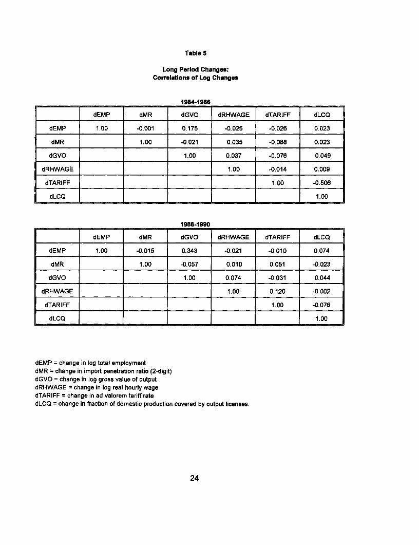
Table 5
Long Period Changes:Correlations ot Log Changes
19841986
dEMP dMR dGVO dRHWAGE dTARIFF dLCQ
dEMP 1.00 -0.001 0.175 -0.025 -0.026 0.023
dMR 1.00 -0.021 0.035 -0.088 0.023
dGVO 1.00 0.037 -0.076 0.049
dRHWAGE 1.00 -0.014 0.009
dTARIFF 1.00 -0.506
dLCQ 1.00
1986-1990
dEMP dMR dGVO dRHWAGE dTARIFF dLCQ
dEMP 1.00 -0.015 0.343 -0.021 -0.010 0.074
dMR 1.00 -0.057 0.010 0.051 -0.023
dGVO 1.00 0.074 -0.031 0.044
dRHWAGE 1.00 0.120 -0.002
dTARIFF 1.00 -0.076
dLCQ 1.00
dEMP = change in log total employmentdMR = change in import penetration ratio (2-digit)dGVO = change in log gross value of outputdRHWAGE = change in log real hourly wagedTARIFF = change in ad valorem tariff ratedLCQ = change in fraction of domestic production covered by output licenses.
24
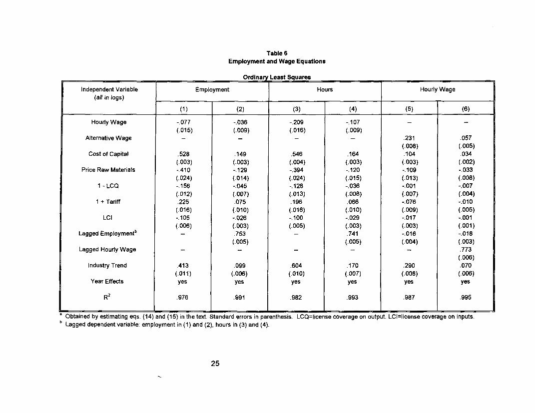
Table 6Employment and Wage Equations
Ordina Least Squares
Independent Variable Employment Hours Hourly Wage
(all in logs) l
(1) (2) (3) (4) (5) (6)
Hourly Wage -.077 -.036 -.209 -.107 -
(.015) (.009) (.016) (.009)Alternative Wage _ _ _ - .231 .057
(.008) (.005)
Cost of Capital .528 .149 .546 .164 .104 .034
(.003) (.003) (.004) (.003) (.003) (.002)
Price Raw Materials -.410 -.129 -.394 -.120 -.109 -.033
(.024) (.014) (.024) (.015) (.013) (.008)
1 -LCQ -.156 -.045 -.128 -.036 -.001 -.007
(.012) (.007) (.013) (.008) (.007) (.004)
1 + Tariff .225 .075 .196 .066 -.076 -.010
(.016) (.010) (.016) (.010) (.009) (.005)
LCI -.105 -.026 -.100 -.029 -.017 -.001
(.006) (.003) (.005) (.003) (.003) (.001)
Lagged Employmentb .753 .741 -.016 -.018
(.005) (.005) (.004) (.003)Lagged Hourly Wage _ _- -_ .773
(.006)
Industry Trend .413 .099 .604 .170 .290 .070
(.011) (.006) (.010) (.007) (.008) (.006)
Year Effects yes yes yes yes yes yes
R 2 .976 .991 .982 .993 .987 .995
' Obtained by estimating eqs. (14) and (15) in the text. Standard errors in parenthesis. LCQ=license coverage on output. LCI=license coverage on inputs.
b Lagged dependent variable: employment in (1) and (2), hours in (3) and (4).
25

Table 6 (cont)Employment and Wage Equations
Joint Estimation (GLS)
Independent Variable Emp. | Wage Emp | Wage Hours | Wage Hours Wage(all in logs) I I l l
(7) (8) (9) (10)
Hourly Wage -.130 - -.035 - -.245 - -.108 -
(.015) (.009) (.016) (.010)Altemative Wage - .222 - .231 - .231 - .231
(.008) (.008) (.008) (.008)Cost of Capital .534 .109 .149 .105 .550 .108 .164 .105
(.004) (.003) (.003) (.003) (.004) (.003) (.004) (.003)Price Raw Materials -.417 -.102 -.129 -.109 -.398 -.111 -.120 -.109
(.024) (.013) (.014) (.013) (.024) (.013) (.015) (.013)1 - LCQ -.159 .036 -.045 -.001 -.128 -.002 -.036 -.001
(.013) (.007) (.007) (.007) (.013) (.007) (.008) (.007)1 + Tariff .224 -.078 .076 -.076 .194 -.074 .067 -.076
(.016) (.009) (.010) (.009) (.016) (.009) (.010) (.009)LCI -.106 -.014 -.026 -.017 -.101 -.017 -.029 -.017
(.006) (.003) (.003) (.003) (.006) (.003) (.003) (.003)Lagged Employmentb - - .753 -.016 - - .740 -.016
(.005) (.004) (.005) (.004)Industry Trend .438 .308 .098 .290 .621 .293 .170 .290
(.011) (.009) (.007) (.008) (.011) (.008) (.007) (.008)Year Effects yes yes yes yes yes yes yes yes
RMSE .734 .414 .437 .394 .737 .394 .452 .394
x2 10.439 10.439 0.004 0.004 5.323 5.323 0.009 0.009
a Obtained by estimating eqs. (14) and (15) in the text jointly via GLS. Standard errors in parenthesis.b x2 test for independence of the employment and wage equation residuals.
26

Table 7Reduced-Form Employment and Wage Equations with Lagged Value Added per Worker
Ordinary Least Squares
Independent Variable Employment Hours Hourly Wage(all in logs)
(1) 1 (2) (3) (4) (5) (6)
Hourly Wage .040 -.005 -.100 -.077 -
(.015) (.008) (.016) (.008)Alternative Wage _ _ _ - .184 .055
(.007) (.005)Cost of Capital .547 .130 .560 .142 .052 .027
(.004) (.003) (.004) (.003) (.003) (.002)Price Raw Materials -.420 -.109 -.428 -.119 -.076 -.031
(.022) (.011) (.022) (.012) (.012) (.008)1 - LCQ -.133 -.029 -.116 -.025 -.007 -.009
(.012) (.006) (.012) (.006) (.006) (.004)1 + Tariff .204 .060 .185 .053 -.047 -.006
(.015) (.007) (.014) (.008) (.008) (.005)LCI -.087 -.016 -.086 -.020 -.034 -.006
(.006) (.003) (.005) (.003) (.003) (.002)Lagged Employmentb .802 .789 .012 -.014
(.004) (.004) (.004) (.003)Lagged Hourly Wage _ _ _- - .741
(.006)Lagged Value Added per -.154 -.043 -.129 -.033 .194 .038
Worker (.008) (.004) (.008) (.004) (.004) (.003).412 .074 .609 .143 .343 .091
Industry Trend (.011) (.006) (.010) (.006) (.008) (.006)yes yes yes yes yes yes
Year Effects.984 .996 .987 .997 .989 .995
R 2
a Obtained by estimating eqs. (14) and (15) in the text. Standard errors in oarAnthesis. LCQ=license coverage on output. LCI=license coverage on inputs.
b Lagged dependent variable: employment in (1) and (2), hours in (3) and (4).
27

Table 8
Ratio of Production Workers to Total Employment
Year All Industries High initial Medium initial Low initialprotection protection protection
1984 .694 .732 ..678 .6761985 .697 .735 .681 .6781986 .688 .728 .672 .6701987 .685 .726 .668 .6661988 .684 .725 .666 .6641989 .683 .727 .663 .6621990 .684 .732 .665 .661
Skilled-Unskilled Wage Differentials(Ratio of wage of non-production workers to wage of production workers)
Year All Industries High initial Mdium initial Low initialprotection protection protection
1984 2.115 1.976 2.116 2.2411985 2.241 2.234 2.217 2.2691986 2.099 2.088 2.031 2.1731987 2.061 2.052 2.042 2.0871988 2.214 2.190 2.262 2.1911989 2.471 2.633 2.328 2.4611990 2.711 2.956 2.567 2.629

Table 9
Employment and Wage Equations, Production vs. Non-Production Workerse
Employment WagesVariable _ ||
Production Non-Production Production Non-Production
Production Wage -.105 .308 .938(.021) (.023) (.010)
Non-Production -.041 -.051 .544Wage (.016) (.017) (.006)
Cost of Capital .517 .541 .018 .040(.004) (.005) (.002) (.003)
Price Raw -.405 -.408 -.063 .021Materials (.026) (.029) (.011) (.014)
Alternative Wage - _ .065 .034(.007) (.009)
1 - LCQ -.131 -.102 -.010 .011(.014) (.015) (.005) (.007)
1 + Tariff .273 .138 -.040 .010(.017) (.019) (.007) (.009)
LCI -.128 -.048 -.015 .001(.006) (.007) (.003) (.003)
Lagged .781 .782 -.005 -.006Employmentb (.005) (.005) (.003) (.004)
Industry Trend .357 .142 .083 .107(.012) (.014) (.007) (.009)
Year Effects yes yes yes yes
RMSE .810 .866 .332 .435
2 4185.9
a Equations estimated jointly via GLS. Standard errors in parenthesis.b X2test for independence of the residuals.
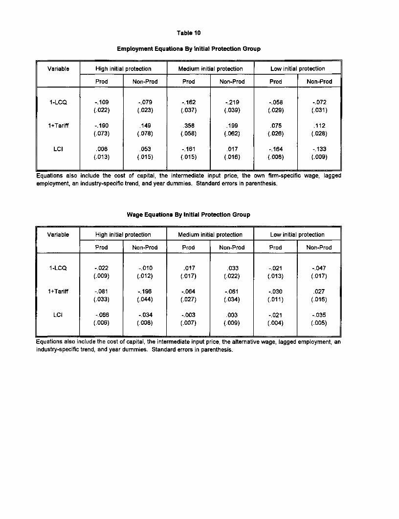
Table 10
Employment Equations By Initial Protection Group
Variable High initial protection Medium initial protection Low initial protection
Prod Non-Prod Prod Non-Prod Prod Non-Prod
1-LCQ -.109 -.079 -.162 -.219 -.058 -.072(.022) (.023) (.037) (.039) (.029) (.031)
1 +Tariff -.190 .149 .358 .199 .075 .112(.073) (.078) (.058) (.062) (.026) (.028)
LCI .008 .053 -.161 .017 -.164 -.133(.013) (.015) (.015) (.016) (.008) (.009)
Equations also include the cost of capital, the intermediate input price, the own firm-specific wage, laggedemployment, an industry-specific trend, and year dummies. Standard errors in parenthesis.
Wage Equations By Initial Protection Group
Variable High initial protection Medium initial protection Low initial protection
Prod Non-Prod Prod Non-Prod Prod Non-Prod
1-LCQ -.022 -.010 .017 .033 -.021 -.047(.009) (.012) (.017) (.022) (.013) (.017)
1+Tariff -.081 -.196 -.064 -.061 -.030 .027(.033) (.044) (.027) (.034) (.011) (.016)
LCI -.066 -.034 -.003 .003 -.021 -.035(.006) (.008) (.007) (.009) (.004) (.005)
Equations also include the cost of capital, the intermediate input price, the alternative wage, lagged employment, anindustry-specific trend, and year dummies. Standard errors in parenthesis.

REFERENCES
Abraham, K. and S. Houseman (1993). "Does employment protection inhibit labor marketflexibility? Lessons from Germany, France and Belgium," NBER Working Paper 4390.
Bentolila, S. and J. Dolado (1992). "Who are the insiders? Wage Setting in SpanishManufacturing Firms," CEPR Discussion Paper 754.
Card, D. (1990). "Employment Determination in Union Contracts," American Economic Review,Vol 80, No. 4, pp. 669-688.
Craig, M. and M. Epelbaum (1994). "The Premium for Skills: Evidence from Mexico". Mimeo,Columbia University.
De Lamo, A. and J. Dolado (1991). "Un modelo del mercado de trabajo y la restriccion deoferta en la economia espainola," Banco de Espaina, Documento de Trabajo 9116.
Feliciano, Z. (1994). "Workers and Trade Liberalization: The Impact of Trade Reforms inMexico on Wages and Employment", unpublished miemo, Harvard University/
Grether, J.M. (1993). "Trade Liberalization, Market Structure and Performance in MexicanManufacturing", Cahiers du Departement d'Economie Politique, Universite de Geneve, No.9308.
Hansen, G. and A. Harrison (1994). "Trade, Technology and Wage Inequality: Evidence fromMexico". Mimeo, University of Texas.
Hufbauer, G. and J. Schott (1992). Prospects for North American Free Trade. WashingtonDC: The Institute for International Economics.
Layard, R., Nickell, S. and R. Jackman (1991). Unemployment: Macroeconomic Performanceand the Labour Market. Oxford: Oxford University Press.
Lindbeck, A. and D. Snower (1988). The Insider-Outsider Theory of Employment andUnemployment. Cambridge, Massachussets: MIT Press.
Revenga, A. (1993). "Wage Determination in an Open Economy: International Trade and U.S.Manufacturing Wages", forthcoming in the Oxford Bulletin of Economics and Statistics.
Tybout, J. and D. Westbrook (1992). "Trade Liberalization and the Structure of Production inMexican Manufacturing Industries", Georgetown University unpublished paper.
Ten Kate, A. (1993). "Trade Liberalization and Economic Stabilization in Mexico: Lessons ofExperience", World Development, Vol. 20, No. 5.

Policy Research Working Paper Series
ContactTitle Author Date for paper
WPS1503 Africa's Growth Tragedy: A William Easterly August 1995 R. MartinRetrospective, 1960-89 Ross Levine 39120
WPS1504 Savings and Education: A Life-Cycle Jacques Morisset August 1995 N. CuellarModel Applied to a Panel of 74 C6sar Revoredo 37892Countries
WPS1505 The Cross-Section of Stock Returns: Stijn Claessens September 1995 M. DavisEvidence from Emerging Markets Susmita Dasgupta 39620
Jack Glen
WPS1506 Restructuring Regulation of the Rail loannis N. Kessides September 1995 J. DytangIndustry for the Public Interest Robert D. Willig 37161
WPS1507 Coping with Too Much of a Good Morris Goldstein September 1995 R. VoThing: Policy Responses for Large 31047Capital Inflows in Developing Countries
WPS1508 Small and Medium-Size Enterprises Sidney G. Winter September 1995 D. Evansin Economic Development: Possibilities 38526for Research and Policy
WPS1509 Saving in Transition Economies: Patrick Conway September 1995 C. BondarevThe Summary Report 33974
WPS1510 Hungary's Bankruptcy Experience, Cheryl Gray September 1995 G. Evans1992-93 Sabine Schlorke 37013
Miklos Szanyi
WPS1511 Default Risk and the Effective David F. Babbel September 1995 S. CocaDuration of Bonds Craig Merrill 37474
William Panning
WPS1512 The World Bank Primer on Donald A. Mcisaac September 1995 P. InfanteReinsurance David F. Babbel 37642
WPS1513 The World Trade Organization, Bernard Hoekman September 1995 F. Hatabthe European Union. and the 35835Arab World: Trade Policy Prioritiesand Pitfalls
WPS1514 The Impact of Minimum Wages in Linda A. Bell September 1995 S. FallonMexico and Colombia 38009
WPS1515 Indonesia: Labor Market Policies Nisha Agrawal September 1995 WDRand International Competitiveness 31393
WPS1516 Contractual Savings for Housing: Michael J. Lea September 1995 R. GarnerHow Suitable Are They for Bertrand Renaud 37670Transitional Economies?
Policy Research Working Paper Series
ContactTitle Author Date for paper
WPS1517 Inflation Crises and Long-Run Michael Bruno September 1995 R. MartinGrowth William Easterly 39120
WPS1518 Sustainability of Private Capital Leonardo Hernandez October 1995 R. VoFlows to Developing Countries: Heinz Rudolph 31047Is a Generalized Reversal Likely?
WPS1519 Payment Systems in Latin America: Robert Listfield October 1995 S. CocaA Tale of Two Countries -Colombia Fernando Montes-Negret 37664and El Salvador
WPS1520 Regulating Telecommunications in Ahmed Galal October 1995 P. Sintim-AboagyeDeveloping Countries: Outcomes, Bharat Nauriyal 38526Incentives, and Commitment
WPS1521 Political Regimes, Trade. and Arup Banerji October 1995 H. GhanemLabor Policies Hafez Ghanem 85557
WPS1522 Divergence. Big Time Lant Pritchett October 1995 S. Fallon38009
WPS1523 Does More for the Poor Mean Less Jonah B. Gelbach October 1995 S. Fallonfor the Poor? The Politics of Tagging Lant H. Pritchett 38009
WPS1524 Employment and Wage Effects of Ana Revenga October 1995 A. RevengaTrade Liberalization: The Case of 85556Mexican Manufacturing