energy efficiency opportunities in industrial
TRANSCRIPT

Page 1
© 2003 Reindl
Energy Efficiency Opportunities in Industrial Refrigeration SystemsEnergy Efficiency Opportunities in Energy Efficiency Opportunities in Industrial Refrigeration SystemsIndustrial Refrigeration Systems
University of Wisconsin-Madison
Douglas T. Reindl, Ph.D., P.E.Director, Industrial Refrigeration ConsortiumUniversity of [email protected]
Learning Objective:The learning objective of this module is to review the common configurations of single and multi-stage vapor compression refrigeration systems that we first studied in the Introduction course. At the end of this segment you should recall the following:
• theory of operation for single stage and two-stage vapor compression refrigeration systems• direct-expansion, flooded, and liquid overfed evaporator configurations• two-stage systems with direct & indirect liquid expansion
---This training module has been developed for presentation at the IIR meeting in Washington, DC, USA by Douglas T. Reindl, Director of the Industrial Refrigeration Consortium at the University of Wisconsin-Madison ([email protected]). It is intended solely for use by short course attendees and may not be reproduced, wholly or partially, without written permission of the author. Please contact the author for information on use ([email protected]).

Page 2
© 2003 Reindl
Our Tasks During This Workshop
Review of systemssingle stage compression systemsmulti-stage compression systems
Performance Analysis (Benchmarking)Energy Efficiency Opportunities
The refrigerant of choice in the industrial sector is anhydrous ammonia; consequently, the materials prepared and data shown in this series of presentations assumes that ammonia is the refrigerant.

Page 3
© 2003 Reindl
Direct-Expansion System
Compressor
Suction trap orReboiler
Expansion Valve
King Valve
EvaporativeCondenser
Hi Pressure Receiver
Evaporator
Equa
lizer
line
1
2
3
External Equalize Line
4
T
Theory of Operation:High pressure and relatively high temperature liquid is drawn from the high pressure receiver and throttled into the evaporator to meet refrigeration loads. The expansion valve (typically a thermostatic expansion device) functions to modulate the flow of refrigerant supplied to evaporator in response to changes in the demand for refrigeration. The demand for refrigeration is determined indirectly by “monitoring” the state of refrigerant superheat at the outlet of the evaporator. Refrigerant superheat is sensed by a temperature-sensitive bulb attached to the evaporator outlet. When the evaporator load increases, the bulb will sense an increase in refrigerant superheat and call for the expansion valve to open; thereby, increasing the supply of refrigerant to the evaporator. As the evaporator load decreases, the refrigerant superheat decreases and the sensing bulb notifies the expansion valve to reduce the flow of refrigerant supplied to the evaporator. If an evaporator is equipped with a refrigerant distributor or if the pressure drop across the evaporator is high (in excess of 2 F saturation temperature equivalent pressure loss which corresponds to about 2 psi at an evaporator temperature of 10 F), then an external equalizing line is needed to properly compensate the temperature sensing bulb. Always connect the equalizer line at the top of the line leaving the evaporator to avoid any oil or other contaminants from clogging the equalizer line.Since expansion valves in ammonia systems are especially prone to “wire-drawing” (accelerated wear of valve’s needle and seat), they require frequent service. In situations where valves are worn, they will not be able to adequately modulate flow at low load conditions; thereby, admitting more refrigerant to the evaporator than is needed for the present load. The net result is an increased likelihood for liquid refrigerant to carry-over to the compressor. To prevent this, a “suction trap” (also known as a “knock-out drum” or “reboiler” is a vessel to separate liquid from vapor prior to compressor suction) is positioned between the outlet of the evaporator(s) and the compressor suction. The trap functions to catch any liquid refrigerant that is carried-over; thereby, protecting the compressor from ingesting liquid refrigerant. A subcooling circuit is typically included in this vessel to boil off any liquid trapped. Alternatively, a number of other liquid transfer methods/strategies can also be applied to the trap. All methods have to limit the accumulation of liquid from the trap to prevent harming the compressor. In addition, many systems have high level alarms and controls to shutdown compressors when the liquid level in the suction trap could endanger the compressors by drawing liquid into the suction line.

Page 4
© 2003 Reindl
Gravity Flooded Recirculation
Suction Trap
Fill float
Evaporator
Surge Drum
King Valve
EvaporativeCondenserEvaporativeCondenser
Hi Pressure Receiver
Equa
lizer
line
1
2
3
4
4’
Solenoidvalve
Hand-expansionvalve
via transfer station (not shown)
Theory of Operation:Low pressure low temperature vapor (state 1) enters the compressor. The compressor raises the pressure of the refrigerant and the superheated vapor travels to the condenser (state 2). Heat is rejected from the refrigerant and, in the process, liquefies (state 3). Saturated liquid refrigerant at high pressure drains into the high pressure receiver. On-demand, the high pressure liquid is “metered” or throttled to the low-side of the system to meet refrigeration requirements. The throttling process is accomplished by a float sensing liquid level. As the liquid level drops, the float will energize a single pole double throw contact that powers open a liquid feed solenoid valve to feed high pressure liquid across a downstream hand-expansion valve. When the liquid level rises to the upper control of the float (usually a 2 inch change in level), the float opens the single pole double throw switch; thereby, closing the solenoid valve by denergizing it.In a gravity recirculation or flooded system, each evaporator is fitted with a surge drum that supplies low temperature saturated liquid refrigerant to the bottom of an evaporator coil (state 4’). As the coil absorbs heat, the refrigerant on the tube-side of the evaporator begins to boil. Since refrigerant, in a vapor state, is significantly lighter than the liquid state, the refrigerant vapor will tend to rise and induce a natural circulation of refrigerant flow upward through the circuits of the evaporator to the outlet line that connects to the vapor space in the surge drum.At sufficiently high loads, the circulation rate through the evaporator could be high enough to entrain and return un-boiled liquid from the evaporator back to the surge drum. Under this operating circumstance, the surge drum serves to separate out liquid and vapor which allows the liquid to recirculate back to the evaporator and the vapor (State 1) to the compressor suction (usually through a transfer station).When the liquid feed solenoid valve is open, the portion of high pressure liquid throttled into the surge drum that flashes to vapor will short-circuit the evaporator and return directly to the compressor suction via the suction trap. The remaining cold liquid falls to the bottom of the surge drum and is made available for circulating through the coil.Typically, a suction trap (also known as a dump trap, trap, knock-out drum) is provided to protect compressors from liquid carry-over. There are a number of possible configurations to return accumulated liquid to the system including gas pumping, mechanically pumped, gravity drain, and others. A dashed line is shown in the figure indicating that any accumulated liquid would be transferred back to the high pressure receiver using the appropriate equipment.

Page 5
© 2003 Reindl
Overfeed System layout
Compressor
Pump
Dry
suction
EvaporativeCondenserEvaporativeCondenser
Hi Pressure Receiver
Equa
lizer
line
EvaporatorEvaporator
Evaporator
2
34’
T
T
Trap
Wetsuction
4’’Low PressureAccumulator
14
Pulse-widthvalve Le
vel p
robe
via transfer station (not shown)
Theory of Operation:In an overfeed system, a refrigerant pump removes cold saturated liquid refrigerant (state 4’) from a low pressure accumulator and pumps it out to a multiplicity of individual evaporators (state 4’’). As evaporators call for refrigeration (usually by a triggered temperature sensor in the refrigerated space or the process being cooled), a solenoid valve will open admitting liquid refrigerant to flow through the evaporator. By design, more liquid refrigerant is pumped through the evaporator than can be evaporated in a single pass - hence the name “overfeed system”. As a result, a mixture of liquid and vapor refrigerant will flow back to the low pressure accumulator through the “wet suction return” lines. The low pressure accumulator functions to separate the refrigerant into its liquid and vapor components. The liquid falls to the bottom of the vessel to be pumped back out to the evaporators while the saturated vapor (state 1) is sent back to the compressor suction. As refrigerant is “consumed” by the evaporators, additional refrigerant is supplied by throttling high pressure liquid into the accumulator. There are a number of alternative strategies that can be used to throttle the high pressure liquid. One strategy is to use a simple fill float. As the liquid level drops, the fill float closes a single pole double throw switch and energizes a liquid feed solenoid valve to throttle high pressure liquid across a hand-expansion valve. A second alternative is to monitor the liquid level using a capacitance probe (sometimes referred to as a “level master”). The capacitance probe signal can be used to drive a “pulse-width modulating” valve that provides continuous liquid make-up to the vessel. As the level in the accumulator drops, the pulse width valve will remain open for longer periods of time increase the make-up rate. As the level rises, the pulse width valve will have a shorter dwell period to decrease the rate of refrigerant make-up to the accumulator. Finally, the capacitance probe can be used to drive a motorized valve. As the level rises, the motorized valve is driven to move in a direction of closing. As the level falls, the motorized valve is driven open.

Page 6
© 2003 Reindl
The need for 2-stage Refrigeration Systems
Lower evaporator temperaturesrequires lower evaporator pressuresleading to increased compressor compression ratios
limitations of specific compression technologiesincreased refrigerant discharge superheat

Page 7
© 2003 Reindl
Two Stage(single temperature, two-stage compression, single stage liquid expansion)
EvaporativeCondenser
Hi Pressure Receiver
Equa
lizer
line
High StageCompressor
Intercooler
Fill float
Low StageCompressor
Evaporator
KingFill float
1
2
3
5’4’
6
LPA
5’
5’’
T
4
7
5
5’
The above figure illustrates a refrigeration system consisting of a single temperature two stage compression with a single stage liquid expansion. The single temperature-level evaporator is configured in a mechanically-pumped overfeed arrangement. Other evaporator configurations are possible as are multiplicity of evaporators.Operation:The high-side of the system is virtually identical to the single stage systems already discussed. Starting from the compressor suction (state 1), intermediate pressure vapor refrigerant is drawn into the compressor and raised in pressure. High pressure superheated gaseous refrigerant leaves the compressor (state 2) and travels to the evaporative condenser. The evaporative condenser rejects heat and liquefies the refrigerant (state 3) storing it in the high pressure receiver. Liquid refrigerant leaving the high pressure receiver follows one of two paths. One path delivers high pressure liquid refrigerant (make-up) to the low pressure accumulator (LPA). The flash gas generated (saturated vapor at state 6) in the throttling process returns to the low-stage or booster compressor working between the lowest pressure in the system and an intermediate pressure in the system. The low pressure saturated liquid (state 5’) is available to be pumped-out to all low temperature evaporators (state 5’’). All vapor generated on the low-pressure side of this system is handled by the booster compressor (at state 6). The booster compressor is responsible for raising the pressure of the refrigerant from the low-side of the system (state 6) to an intermediate pressure (state 7). Since the discharge state of the refrigerant from the booster compressor is superheated (even though it is at an intermediate pressure), it must be cooled (or desuperheated) prior to raising its pressure from the intermediate system pressure to the system condensing pressure. The job of desuperheating the discharge gas from the booster compressor(s) is accomplished by the intercooler. In other words, the total heat of rejection on the low-temperature side of the system is imposed or becomes a load on the intercooler. Cool liquid refrigerant (state 4’) in the intercooler absorbs that total heat of rejection and boils to meet the heat load placed on it by the boosters. The level of liquid refrigerant in the intercooler is maintained by throttling additional liquid in from the high-pressure receiver. The high-stage compressor draws intermediate pressure saturated vapor (state 1) from the intercooler and raises its pressure to the system condensing pressure. In the system arrangement shown above, there are two sources of flash gas generation in the intercooler. The first is a consequence of dumping the total heat of rejection from the low-side of the system into the intercooler and the second is a result of throttling high-pressure liquid into the intermediate pressure of the intercooler.Comments:In the above system arrangement, we pay a penalty for throttling the high-pressure liquid directly to the low-side of the system. An alternative would be to first throttle liquid into the intercooler then throttle liquid from the intercooler to the LPR. This can significantly improve system efficiency for low pressure (temperature) systems since the liquid being throttled to the LPR is precooled as a result of originating from the intercooler rather than the high-pressure receiver. The next system diagram shows this change.

Page 8
© 2003 Reindl
Two Stage(single temperature, two-stage compression, two stage liquid expansion)
EvaporativeCondenser
Hi Pressure Receiver
Equa
lizer
line
High StageCompressor
FlashIntercooler
Fill float
Low StageCompressor
Evaporator
KingFill float
1
2
3
44’5’
67
LPA
T
5’’
5
The above figure illustrates a system with single temperature two stage compression and two stage direct liquid expansion. The system operation is similar to that discussed for the single liquid expansion with one important exception. All the liquid make-up to the low-pressure accumulator (LPA) now comes from the intercooler. This precooled liquid reduces the fraction of liquid that flashes to vapor in the LPA and improves system efficiency.

Page 9
© 2003 Reindl
Two Stage System(two temperature level, two-stage compression, two stage liquid expansion)
EvaporativeCondenser
Hi Pressure Receiver
Equa
lizer
lineHigh Stage
Compressor
DirectFlash
Intercooler
Fill float
Low StageCompressor
King
1
2
3
45’
67
LPA
T
5’’
Lo TempEvaporator
Hi TempEvaporator
5
4’Fill float
The above figure illustrates a two-temperature level two stage compression with a two stage direct liquid expansion. The system operation is similar to that discussed for the single temperature two-stage liquid expansion system but in this case, we have refrigeration requirements at the intermediate pressure (temperature) of the system. The evaporators could be configured as DX,flooded, or overfeed in this arrangement.

Page 10
© 2003 Reindl
Two Stage System(two temperature level, two-stage compression, single stage indirect liquid expansion)
Hi Pressure Receiver
Equa
lizer
lineHigh Stage
Compressor
IndirectFlash
Intercooler
Fill float
Low StageCompressor
KingFill float5’
LPA
T
Low TempEvaporator
Hi TempEvaporator
EvaporativeCondenserTXV
1
2
3
45’
67
5’’
5
4’
The above figure illustrates a two-temperature level, two stage compression with indirect liquid expansion. The system operation is similar to that discussed for the single temperature two stage direct liquid expansion system but in this case, we have a heat exchanger immersed below the liquid level in the intercooler. The heat exchanger serves to subcool the high-pressure liquid prior to throttling it to the low-side of the system. Although this is an improvement over the single stage direct expansion arrangement, it suffers slightly worse performance when compared to the two-stage direct case shown previously. The principle reason for slightly worse performance lies in the fact that the liquid being expanded to the low temperature evaporator will not be as cool as if liquid was taken directly from the intercooler (due to limitations of the heat exchanger). As a result, the indirect liquid expansion system will have a greater percentage of flash gas relative to the direct liquid expansion case. The principle advantage of the indirect liquid expansion case lies in the greater degree of subcooling obtained in the high pressure liquid. This subcooling will counter pressure drops in long liquid line runs. Again, the evaporators could be configured as DX, flooded, or overfeed in this arrangement.A significant disadvantage of an indirect-intercooler is that repairing a leak in the heat exchanger is virtually impossible (not to mention the havoc it wreaks on your system when that heat exchanger springs a leak). Although heat exchanger leaks for indirect intercoolers are not a frequent occurrence, they have happened. Another possible method to accomplish subcooling the high press liquid is toconfigure an external subcooling heat exchanger (consider it an evaporator). The high pressure liquid flows through the tube side and the cold liquid from the intercooler flows on the shell-side. In this arrangement, repairing or replacing the heat exchanger can be accomplished without scrapping the intercooler vessel. It is a nice method for generating high pressure subcooled liquid.

Page 11
© 2003 Reindl
Let’s Look at Performance Analysis

Page 12
© 2003 Reindl
Is your system “efficient”?
Compared to what?
A challenge in evaluating energy efficiency for industrial refrigeration systems is the fact that each one is a custom-engineered field-erected system. This makes cataloging system performance impossible. As a result, evaluating their performance is difficult and challenging. We will look at some of the factors that influence the performance of industrial refrigeration systems as a preface to investigating opportunities to improve their efficiency.

Page 13
© 2003 Reindl
Performance Analysis Helps You:
Compare a system's efficiency to others
Determine the cost of refrigeration
Assess a system's ability to meet added loads
Quantify benefits of system modifications
Verify predicted performance was achieved

Page 14
© 2003 Reindl
Measures of Performance
EfficiencyCOP, BHP/ton
Capacity or productivitytons of product manufactured per hr or per day
Annual energy cost$ per year
Normalized energy cost$ per ton of product manufactured
There are a number of possible methods and quantities that can be organized to quantify the performance of a refrigeration system. In some cases, it may make sense to quantify system performance based on an efficiency expressed as the total brake horsepower (BHP) divided by the system refrigeration capacity (expressed in units of tons). In other cases, it may be appropriate to determine the total productivity of a refrigeration system in terms of the tons of cold or frozen product manufactured per hour or per day. Financial managers might be inclined to look only at the annual energy cost for refrigeration. As we will see later in this section, this measure alone can be very deceiving. In a manufacturing environment, it is often preferred to express the annual cost by dividing the energy cost by the total product manufactured.

Page 15
© 2003 Reindl
Efficiency
Engineering definition:"the ratio of the useful output to the energy input to a process or machine“
General usage:the relationship between useful output and purchased input
Refrigeration:typically COP or hp per ton
Whenever you talk about the term “efficiency”, it usually represents what you get out over what you put in. Take a boiler for example. An efficiency rating of 75% for a boiler represents the useful output (steam flowing at the required conditions) divided by the amount of energy input (in the form of a fuel such as natural gas).
In general, an efficiency is expressed in terms of a useful output (e.g. number of pizzas produced) divided by the maximum theoretical output if the line ran at its maximum speed without interruption.
For refrigeration systems, the efficiency is often quantified as the total horsepower input (compressors, condenser fans, condenser water pumps, refrigerant pumps, and evaporator fans) divided by the actual tons of refrigeration produced. In general, measuring the refrigeration-related electrical energy in a plant is simple. The difficult quantity to measure is the tons of refrigeration. Often, other quantities besides “tons of refrigeration” may be tracked such as “tons of hot dogs”, “millions of pizzas”, etc. This process of selecting a quantity to divide into the total work input to the system is often called “normalization”. Selecting an appropriate normalizing variable is often the difference between having a meaningful measure of system performance and having a measure that is useless.

Page 16
© 2003 Reindl
Component vs. System Efficiency
Efficient components does not necessarily mean an
efficient system
Energy use is primarily determined by system
configuration andoperation
You should be interested in SYSTEM performance since the operating cost of refrigeration system is dependent on the efficiency of all components – not just one. It is possible to select and install the most efficient system components but that is no guarantee that the operation of those components when put together in a system will be efficient. As we will see, the interaction of components greatly influences how the system as a whole operates.

Page 17
© 2003 Reindl
Instantaneous vs. Long-term EfficiencyAnnual efficiency is not the same as performance at design conditions
Variations in loadsCompressor part-load performanceCompressor sequencingHead pressure control
Many of the components in a refrigeration system have efficiency characteristics that are variable. We have already looked at how changing head pressure can significantly influence the HP/ton of a compressor. We will look at the performance of compressors are part-load conditions in a future chapter.

Page 18
© 2003 Reindl
Capacity
Possibly the most important performance measure
measure of useful refrigeration
more capacity means more production capability
Efficiency improvements often increase capacity

Page 19
© 2003 Reindl
Annual Energy Cost
Bottom-line measure of refrigeration system efficiency
However,Comparisons should consider
WeatherProductionUtility rates

Page 20
© 2003 Reindl
Annual Energy Cost Example
200000
300000
400000
500000
600000
700000
800000
N-93 M-94 N-94 M-95 N-95 M-96 N-96 M-97 N-97200
400
600
800
1000
1200
1400
1600
1800M
onth
ly E
nerg
y Us
e (k
Wh)
Mon
thly
Pea
k D
eman
d (k
W)
Month
We conducted an investigation aimed at improving the energy efficiency of a doughnut factory. Our visit was prompted by the large increase in energy usage by the plant during the prior four years. When we arrived, we reviewed energy cost and energy use data during the previous five years. The energy use and demand of electricity for the facility had in fact increased during the prior four years. In fact, the demand increased from six hundred kW to well over 1200 kW. The monthly electrical usage increased from approximately 300,000 kWh per month to over 700,000 kWh/month.

Page 21
© 2003 Reindl
Normalized Energy Cost
0
500000
1000000
1500000
2000000
2500000
3000000
N-93 M-94 N-94 M-95 N-95 M-96 N-96 M-97 N-97$0.0000
$0.0050
$0.0100
$0.0150
$0.0200
$0.0250
$0.0300
$0.0350
$0.0400M
onth
ly P
rodu
ctio
n (d
oz)
Mon
thly
Uni
t Ele
ctric
Cos
t ($/
doz)
Month
After pressing the vice president of manufacturing for more details on production, we developed the above graph. First, the monthly production of doughnuts over the prior four years rose substantially. Over the same time period, the unit cost ($ per dozen doughnuts) dropped by more than 50%.

Page 22
© 2003 Reindl
Factors Affecting Performance
A refrigeration system’s performance is affected by:
Loads and the system’s response to meet the loads

Page 23
© 2003 Reindl
Factors Influencing Refrigeration Loads
WeatherMix of productsProduction ratesProduction schedulesProcess constraintsOperating procedures

Page 24
© 2003 Reindl
Factors Influencing System Response
WeatherSystem designOperating proceduresEquipment performance

Page 25
© 2003 Reindl
Weather Influences on Loads
Weather affects:cold storage warehousesrefrigerated docksblast freezing systems in unconditioned production areas
Weather has minimal effect on:many food processing applicationsindustrial process cooling

Page 26
© 2003 Reindl
Weather Influences on the System
Evaporative condensingsensitive to outside air wet-bulb temperaturelower system head pressure
Air-cooled condensingsensitive to outside air dry-bulb temperaturehigher systems head pressure

Page 27
© 2003 Reindl
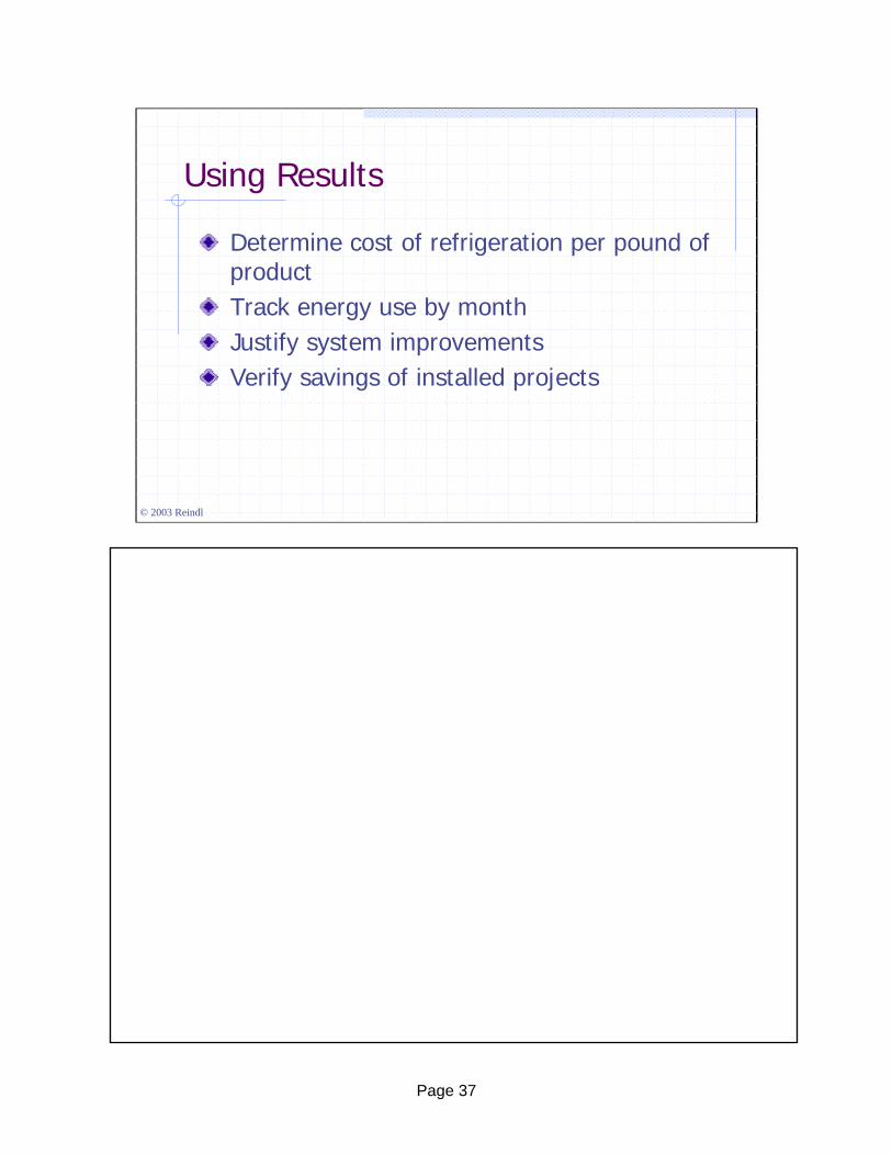
Using Results
Determine cost of refrigeration per pound of productTrack energy use by monthJustify system improvementsVerify savings of installed projects

Page 28
© 2003 Reindl
Benchmark Comparisons -Refrigerated Warehouses
0
2,000,000
4,000,000
6,000,000
8,000,000
10,000,000
12,000,000
0.00 1.00 2.00 3.00 4.00 5.00 6.00 7.00 8.00
volume, million cu ft
kWh/
yr
Since our refrigeration systems do not come with a “MPG” meter, we are stuck trying to identify appropriate measures for quantifying system performance. Once we have those measures quantified, how do we know whether or not the energy use is out of line with what can be expected.We have been looking hard to start a database of energy use statistics. As this database matures, owners can quickly ascertain whether or not their facility is performing at a reasonable level. The above plot shows the annual energy use of refrigerated warehouses according to their size. This plot, by it self, does not provide a completely clear picture.

Page 29
© 2003 Reindl
Benchmark Comparisons -Refrigerated Warehouses
0.0
0.5
1.0
1.5
2.0
2.5
3.0
3.5
4.0
4.5
5.0
0.00 1.00 2.00 3.00 4.00 5.00 6.00 7.00 8.00
volume, million cu ft
kWh/
cu ft
-yr
Taking the previous data and normalizing the energy use by including the warehouse size leads to the above plot. In this case, it appears that the annual energy use on a per cubic foot basis is relatively constant at approximately 1.3 kWh/ft3-yr. If you owned the warehouse that consumed 4.5 kWh/ft3-yr, would you be convinced that opportunities to improve the efficiency of the facilities’ refrigeration system abound?

Page 30
© 2003 Reindl
Billing Analysis
Review 1-3 years’ monthly utility bills Look at demand and energy use profilesSeasonal, month-to-month, year-to-year variations

Page 31
© 2003 Reindl
Billing Analysis Example - Warehouse
0
100,000
200,000
300,000
400,000
500,000
600,000
700,000
800,000
Nov-99 Feb-00 May-00 Aug-00 Nov-00 Feb-01 May-01 Aug-01
Ener
gy U
se [k
Wh]
-
500
1,000
1,500
2,000
2,500
Dem
and
[kW
]
Energy (kWh)
Demand (kW)

Page 32
© 2003 Reindl
Billing Analysis – Dairy Plant
-
100,000
200,000
300,000
400,000
500,000
600,000
700,000
Aug-99 Dec-99 Mar-00 Jun-00 Oct-00 Jan-01 Apr-01 Jul-01 Nov-01
Con
sum
ptio
n [k
Wh]
0
500
1000
1500
2000
2500
3000
Dem
and
[kW
]
Consumption(kWh)Demand (kW)

Page 33
© 2003 Reindl
Isolating Refrigerating System Energy
Estimate use for other loads:lightingBattery chargersAir compressorsProduction equipmentUnderfloor heatOffices
Consider peak load, partial load and schedule of operation

Page 34
© 2003 Reindl
End-Use Breakdown
Compressors21%
Heaters52%
Pumps12%
Air compressor14%
Lights, misc1%

Page 35
© 2003 Reindl
Normalizing Results
Account for variations in weather, production rates, etc.For example:
$/ft2·degree dayEnergy cost per unit producedkWh per square foot

Page 36
© 2003 Reindl
Accounting for Weather Influences
Does system performance depend on weather?Do outside air conditions influence system loads?If “yes” to either question, normalize to account for weatherAverage monthly temperature, degree-days, other
Page 37
© 2003 Reindl
Using Results
Determine cost of refrigeration per pound of productTrack energy use by monthJustify system improvementsVerify savings of installed projects

Page 38
© 2003 Reindl
Uncovering Energy Efficiency OpportunitiesUncovering Energy Efficiency OpportunitiesUncovering Energy Efficiency Opportunities
Learning Objective:The objective of this program segment is to provide you with a ideas for energy efficiency improvements to your systems. At the end of this program segment you should understand the following:
• the need for baselining the performance of your systems• Energy efficiency improvement strategies and their impact potential• importance of following-up after implementation to insure energy improvement targets are met
Upon completion of this program segment you should be able to:• determine appropriate benchmarks for industrial refrigeration systems• consider, evaluate, implement, and verify energy conservation measures based on a range of potential
candidate approaches

Page 39
© 2003 Reindl
Barriers to Realizing Efficient Systems
“Selecting efficient componentsleads to efficient systems – right?”
“I can’t afford to design an efficient system”
“The owner does not want an efficient system”
As I continue working in the area of energy efficiency and industrial refrigeration systems, I find it interesting to hear all of the reasons why efficiency improvements are not possible with “my system”. There are a lot of fallacies out there. One owner that I talked to had a brand new refrigeration system. After looking over the drawings for a short time and talking with the system operators, I was convinced that the system, in its current state, could stand for some changes to improve its efficiency. I went back and asked the owner – “In your opinion, what are the strengths of your current system?” One of the first items stated by the owner was that he had an efficient system. I asked the owner how he knew he had an efficient system. After thinking for a moment, he responded – “I don’t know but I think the system is pretty efficient”.This owner shares a lot in common with other owners. In order to assess efficiency of a system, it is absolutely essential to have performance benchmarks or reference points. Without a reference point, you cannot possibly make accurate statements about the efficiency of a system. In addition, benchmarking your system is critical to determine whether or not changes that are made to improve system efficiency have had the desired effect.

Page 40
© 2003 Reindl
Barriers to Realizing Efficient Systems
The owner can’t afford an efficient system
Energy is too cheap – not cost-effective
“I don’t know how”

Page 41
© 2003 Reindl
Establishing Efficiency Improvement GoalsWhat are the steps?
1. baseline the performance of the current system2. compare baseline w/benchmarks (competitors, published, …)3. identify potential opportunities4. estimate impact/benefit to system5. estimate capital cost6. assess operational risks/constraints7. prioritize by greatest benefit to cost8. follow-up, quantify benefit, & continuously improve
With a solid understanding of the basic system types and their operation as well as utility rates and benchmarking, your are now ready to take the next step. The next step is to pursue, identify, and implement energy conservation measures (ECMs). Upon implementing ECMs, you should follow-up and verify that the savings you have projected are actually being realized. This is a fundamental element of any quality improvement process.

Page 42
© 2003 Reindl
Where are the opportunities?
Floating head pressure control
Oversize evaporative condenser
Raise suction pressure
Compressor selection & operational sequencing
Intercooler pressure reset (two-stage systems)
Convert gas-pumped systems to mechanically-pumped
CompanionStrategies
Let’s look at a long list of potential energy conservation measures. Many of the results and analyses presented in this section are based on past projects that we have tackled. Some of the energy conservation measures are very cost-effective to implement while others are not so financially attractive. We will not have sufficient time to cover all of these opportunities in depth. We will cover as many as time allows.
The first two strategies above: floating head pressure and oversized evaporative condensers can be considered “companion strategies”. For example, it would be foolish to install an oversized evaporative condenser(s) and not lower the system’s head pressure.
Page 43
© 2003 Reindl
Where are the opportunities?
Eliminate or reduce parasitic losses/gains
Defrosting (improved methods & optimized strategies)
Reduce envelope & infiltration loads
Break-out suction levels (eliminate EPRs)
Secondary fluid system improvements
High efficiency motors
Liquid/Flash gas management

Page 44
© 2003 Reindl
Where are the opportunities?Single stage vs. multi-stage systems
Thermal energy storage (passive & active)
Better system integration
Pipe sizing & valve selection (esp. suction side)
Maintenance-related issues
Suction gas desuperheating
Liquid subcooling
Oil cooling strategies
The remainder of this section will examine each of these energy efficiency improvement strategies in more detail. Review them all carefully and then take one and proceed with evaluating and implementing the ECM. Finally, follow-up with verifying that the projected savings are actually being realized.

Page 45
© 2003 Reindl
Head Pressure Control
45

Page 46
© 2003 Reindl
Head Pressure Control
How do we control head pressure in industrial refrigeration systems?
Recall, system head pressure is a controlled variable. We control head pressure by changing the system’s heat rejection rate. Increasing the heat rejection rate causes the head pressure to drop while decreasing the heat rejection rate will cause the head pressure to rise. Systems will have controls and control sequences to maintain system head pressure at a target level.Typically, systems have a head pressure control set-point such as 150 psig (a saturation temperature of 84 F). Controls will modulate the capacity of the heat rejection system in attempts to maintain the head pressure at or near the desired setpoint. Depending on the available heat rejection capacity, the evaporative condenser may or may not have sufficient capacity to reject heat from the system and achieve the head pressure setpoint. For example, let’s assume that our evaporative condenser has an approach temperature (difference in temperature between the saturated condensing refrigerant and the outside air wet bulb temperature) of 18 F. This means that if the outside air wet bulb is 68 F, the saturated condensing temperature would be no lower than 86 F (or ~155 psig). In this case, the evaporative condenser would be running at its maximum capacity and the setpoint condensing pressure would not be satisfied until the outside air wet bulb temperature drops further.At low outside air wetbulb temperatures, the evaporative condenser would have excess capacity. In this case, the effective capacity of the evaporative condenser(s) needs to be modified to maintain the head pressure in a desired range. The following are methods used for modulating condenser capacity: on/off single speed fan control. two-speed fan control, and variable speed fans.For the first two options, a deadband around the desired system head pressure set-point is established e.g. 3 psi. For the single speed fan option, as the head pressure rises to the upper range of the deadband (in this case 153 psig), the condenser fan(s) are energized; thereby, increasing the heat rejection capacity and driving the head pressure down until it reaches the lower deadband limit (147 psig) at which time the condenser fans are cycled off. With the two-speed fan option, the control strategy is basically the same. From an energy perspective, the two-speed fan offers benefits as it attempts to maintain head pressure below the upper deadband by first cycling fans on low-speed and if head pressure continues to rise cycling on fans to high-speed. Since the fan horsepower varies with the cube of the fanspeed, any reduction in fan speed can result in considerable fan horsepower savings.The third option is a variable speed fans. In this case, the fan speed is modulated (from its minimum to its maximum) to maintain the desired head pressure. This option offers the benefits of stable head pressures and most efficient condensing performance; however, it comes at a cost premium over the discrete fan speed options.

Page 47
© 2003 Reindl
Head Pressure Control
Our heat rejection system controls head pressure
Evaporative condenser fan controlson/off (single speed fans)
two-speed fans
variable speed fans

Page 48
© 2003 Reindl
Design Condensing Pressure
Most common design pressure196 psia [1,351 kPa] (95 F [39 C] saturation temperature)
Alternatives to consider181 psia [1,248 kPa] (90 F [32 C] saturation temperature)
good for cold climates and situations that allow head pressure to float during most months of the year
167 psia [1,151 kPa] (85 F [29 C] saturation temperature)good for moderate to cold climates and system designs that allow head pressure to float during most months of the year

Page 49
© 2003 Reindl
Control Options
Single speed fan with on/off controlmost common method of head pressure controlneed to set cut-in (e.g. 150 psig [1,138 kPa]) & cut-out pressures (e.g. 145 psig [1,103 kPa])simple control method but results in
higher energy consumption compared to two-speed or variable speedhigher maintenance (fan motors & belts)liquid management problems in multiple condenser systems

Page 50
© 2003 Reindl
Control Options – Cont.2-Speed fan control
need to set high speed cut-in (e.g. 160 psig [1,207 kPa]), low-speed cut-in pressure (e.g. 150 psig [1,138 kPa]), and low-speed cut-out pressure (e.g. 145 psig [1,103 kPa])
relatively simple control method but results inhigher capital cost compared to single speed fan option
lower energy consumption compared to single-speed but slightly higher energy consumption compared to variable speed
liquid refrigerant management problems with multiple condensers
cycling results in less system transients compared to single speed
sequencing speed controls requires attention

Page 51
© 2003 Reindl
Control Options – Cont.Variable frequency drive
need to set a target head pressure and fan speed is modulated to maintain head pressure
a very simple principle and method to implementhighest capital cost alternative
lowest energy consumption control alternative
should modulate all condensers the same in systems with multiple evaporative condensers
results in smoother system operation with minimal transients

Page 52
© 2003 Reindl
Condenser Fan Control Map
Strategy Mode 1 Mode 2 Mode 3 Mode 4 Mode 5Small Motor off on off onLarge Motor off off on onSmall Motor off off onLarge Motor off on onSmall Motor off on on onLarge Motor off off half-speed onSmall Motor off half-speed half-speed on onLarge Motor off off half-speed half-speed onSmall Motor offLarge Motor off
5 variable speedvariable speed
1
2
3
4
The above map provides five different strategies that could be used for an evaporative condenser that is equipped with twin motors, two-speed fans, or variable speed fans. The “modes” are indicative of changes in head pressure (either increasing as one moves from left to right or decreasing as one moves from right to left).For example, strategy 3 would work as follows. In mode 1 all fans are off. As the head pressure rises, the system responds by energizing a small fan motor in attempts to maintain system head pressure. If the head pressure continues to rise and the setpoint is not satisfied, mode three is initiated by the start of the larger fan motor to half-speed. As the head pressure rises further, mode 4 dictates that the larger fan motor is tripped to run at high speed. The exact opposite sequence occurs as the head pressure falls.

Page 53
© 2003 Reindl
Condenser Fan Control Options
The above figure illustrates the required fan energy (expressed as a percentage of full-load fan power) as a function of the evaporative condenser capacity for the five strategies listed previously. The least efficient option is the on/off control (strategy 1) while the most efficient option is the variable speed drive option. The two-speed fan option yields nearly all of the part-load power and capacity benefits of the variable speed option but with much less costly equipment.Notice that at zero fan power for all options, the capacity of the evaporative condenser is not zero. This is due to the fact that natural convection will occur drawing air through the condenser coils and rejecting heat yielding about 10% of the condenser’s heat rejection capacity while the fans are idle. This assumes that the condenser coils are running wet i.e. water continues to flow over the condenser coils.

Page 54
© 2003 Reindl
Floating Head Pressure Control
This strategy:
allows head pressure to drop with decreasing outside air wet bulb temperature
takes advantage of excess evaporative condenser capacity during cool outside air conditions
head pressure allowed to drop to a pre-determined minimum (for example Pcond,min = 110 psig [862 kPa])
Floating head pressure control is an ECM that often has the greatest cost/benefit when compared with other ECMs for a wide range of system types. All too often, systems in the field operate with excessively high head pressure leading to higher than nessary operating costs.The above items describe the “whats” of floating head pressure control. The thing to realize is that all systems have “floating head pressure” to some extent. Many systems are controlled to artificially maintain head pressures high (150 psig or higher) year-’round regardless of outside air temperatures.An extreme example of this is the ice arena case study that we will discuss. This R22 system had its controls to maintain head pressure between 220-235 psig year-’round (this corresponds to a condensing temperature of between 108-113 F!). Not only was this system using an excessive amount of energy, the compressor’s life will be shortened considerably as a result of being forced to work overtime year-’round. The belts on the evaporative condenser fans as well as the motors had their lives shortened as well due to the extreme short-cycling of the evaporative condenser fans during cold outside air temperatures. This system’s head pressure was reset to 150 psig without any adverse problems yielding significant energy and maintenance cost savings.

Page 55
© 2003 Reindl
Floating Head Pressure Control
Consequences of lowering head pressure
increased evaporative condenser energy usage
decreased compressor energy usage
reduced high stage compression (on average)

Page 56
© 2003 Reindl
Floating Head Pressure Control
Benefitsimproved system efficiency
~1.3% for each °F reduction in saturated condensing temperature
increased system capacity
compressor life is prolonged
oil cooling loads decrease
The above items outline the benefits or the “whys” of floating head pressure control.As a rule-of-thumb, you can expect that a compressor will realize about a ~1.3% improvement in efficiency (BHP/ton) for each degree lower in condensing temperature. For example, a compressor operating at 0 F (15.7 psig) saturated suction temperature and 95 F (180 psig) saturated condensing temperature would operate at about 1.68 BHP/ton. If the condensing temperature were allowed to decrease to 85 F (152 psig), the compressor would now operate at 1.46 BHP/ton - nearly a 13% improvement in compressor efficiency. The actual compressor performance enhancement with lower condensing temperatures will depend on the compressor technology (reciprocating, screw, etc.) and its individual performance character.The “hows” of implementing floating head pressure control will be discussed next including limitations. Basically, floating head pressure control is as simple as resetting the condensing pressure control setpoint (every system has one).

Page 57
© 2003 Reindl
Optimum Head Pressure
82 84 86 88 90 92 94 960
20
40
60
80
100
120
140
160
Saturated Condensing Temperature (F)
Pow
er (k
W)
Compressor
Compressor+Condenser
Condenser
Axial Fan
Tcond,opt = 87.1 F
Toa,wb=78°F

Page 58
© 2003 Reindl
Optimum Head Pressure
82 84 86 88 90 92 94 960
50
100
150
200
250
300
Saturated Condensing Temperature (F)
Pow
er (k
W)
Centrifugal Fan
Compressor
Compressor+Condenser
CondenserTcond,opt = 89.9 F
Toa,wb=78°F

Page 59
© 2003 Reindl
Floating Head Pressure ControlHead pressure limits dictated by:
hot gas defrost requirementssetting of defrost relief valvessizing of hot gas maincondensate management in hot gas main
DX evaporatorsmost thermostatic expansion valves need at least 75 psig [517 kPa] differential pressure to function properly
liquid injection oil coolingcheck manufacturer’s requirements for TXV pressure differential
As with most things, there are limits to lowering system head pressure. We do not want to create problems by trying to improve the efficiency of our systems. The above items are some of the more common factors constraining or limiting our ability to lower system head pressure. Keep in mind that these items may not necessarily be unmovable barriers; however, changes in components or system arrangements may be required to overcome their limiting effects on the system.Hot Gas Defrost:Many industrial refrigeration systems utilize hot gaseous refrigerant to defrost evaporators. In cases where defrost relief valves are installed, a sufficient pressure differential (e.g. 75 psig) across the valve must be created to open the valve. Sizing of the hot gas main may also impose constraints. If a hot gas main is undersized, hot gas (at a sufficient rate) will not be delivered to the evaporator without a high differential pressure. For larger size hot gas mains, a much lower differential pressure will allow adequate flow of hot gas to defrosting evaporator(s). Finally, if condensate is not properly managed in hotgas mains, hydraulic shock can cause catastrophic failures of hot gas piping on a call for defrost. Also, the condensate effectively decreases the pipe size causing similar symptoms as an undersized line with regard to head pressure requirements. All of these deficiencies can be overcome in the long run; however, they do create real barriers to lowering head pressure in the short run.DX Evaporators:In systems that utilize direct-expansion evaporators, a minimum differential pressure is required across the thermostatic expansion valves (TXV). The minimum pressure differential is dependent on the specific valve selection but is routinely on the order of 75 psig. When we drop the pressure differential across the TXV below the minimum, we lose controllability of the valve (control engineers call this “control authority”). What results is an inability to properly modulate refrigerant to the evaporator. Since our evaporator pressure i.e. downstream of the TXV the pressure is fixed (to satisfy our temperature requirements for meeting load), the head pressure i.e. upstream of the TXV is limited in its ability to float. If we have DX evaporators on a dock being controlled to 48 psig (32 F saturation temperature), our minimum head pressure would be in the range of 123 psig (48 psi+75 psi).LIOC:Liquid injection oil cooling (also commonly referred to as SOC or screw oil cooling) utilizes high pressure liquid and expands it directly (using TXVs) into the compressor to accomplish oil cooling in screw compressors. The TXVs for liquid injection oil cooling tend to be small and require larger pressure differentials for controllability – usually on the order of 100 psi. This further limits many screw compressor’s from floating head pressure. One approach for circumventing this limitation is to utilize thermosiphon oil coolers (TSOC).

Page 60
© 2003 Reindl
Floating Head Pressure ControlHead pressure limits dictated by:
evaporative condenser selectionoversized evaporative condensers usually result in an optimum head pressure that depends on outdoor air temperature (more on this momentarily)
evaporative condenser fan controlsVFD fans are preferred but 2-speed fans yield considerable benefits
Evaporative Condenser Selection:If an evaporative condenser is too small, the system head pressure will rise until its heat rejection capacity is sufficient to reject the needed heat from the system.
Fan Controls:Although fan controls themselves do not necessarily limit head pressure, there are methods of fan controls that lead to more stable and efficient system operation. Two speed condenser fans or variable frequency drive (VFD) fans have better capacity modulating capability and result in more stable head pressures – leading to more stable system operation. In addition to their stability, two-speed and VFD controlled fans will result in improved energy due to their better part-load performance as compared to single speed fans.
Thermosiphon Oil Cooling (TSOC):TSOC improves compressor efficiency by using a thermosiphon effect coupled with the system’s evaporative condenser to reject heat from the compressor’s oil.

Page 61
© 2003 Reindl
Floating Head Pressure ControlHead pressure limits dictated by:
hand expansion valve settingssignificantly lowering head pressure will likely require seasonal HEV adjustmentsthis constraint can be overcome by the use of motorized valves or pulse width valves
oil separator sizinggas driven systems (transfer systems and gas pumpers)controlled-pressure receiver setpointsheat recoveryengineering and operations (knowledge and willingness)

Page 62
© 2003 Reindl
Case Study: Madison Ice ArenaNew system (1996) City-owned and operatedRink is operated year-’roundCapacity of 103 tonsSix compressors: max power = 240 kWRefrigerants R22 and ethylene glycolEvaporative condenserAnnual electrical operating cost: $45,600
Just another case study to illustrate the impacts of head pressure and head pressure control on system performance. This particular system consists of a built-up refrigeration system that serves a local municipal ice arena. The system consists of two separate refrigeration circuits using R-22 as the refrigerant. Ethylene glycol moves through a common shell-and-tube evaporator with two refrigerant direct-expansion refrigerant circuits. Each circuit is served by three Carrier Carlyle reciprocating compressors (i.e. a rack) operating in parallel.When we started on the project, the system was approximately one year old (a renovation) and the owner (City of Madison) was disappointed that operating cost savings had not reached expected levels. We were invited to evaluate the system and make recommendations to the owner for improving the system performance, efficiency, and operating costs. As we will see shortly, the single largest opportunity to reduce energy costs in this system involved a head pressure reset.(NOTE: This case study was conducted by Brownell, K. A. in partial fulfillment of the requirements for a MS degree in Mechanical Engineering under the direction of Professor’s Reindl, D. T., and Klein, S.A. during 1997-1999. Portions of the thesis prepared by Brownell titled “Investigation of the Field Performance for Industrial Refrigeration Systems”, 1998 have been excerpted in this case study. A complete copy of the Brownell thesis is available for download at: http://www.irc.wisc.edu/publications

Page 63
© 2003 Reindl
Case Study: Madison Ice ArenaAs-installed, head pressure controlled 220-235 psig [1,620 – 1,724 kPa]Proposed: allow condenser pressure to ‘float’ with varying outdoor temperatureLow pressure limit reset to 150 psig [1,138 kPa]
required change: fan controller setpointAdvantages
quieter; lower maintenance21% operating cost savings $9,600/yr

Page 64
© 2003 Reindl
Oversized Evaporative Condensers
64

Page 65
© 2003 Reindl
Oversizing Evaporative Condensers
Design point (historical)95 F [35 C] saturated condensing temperature (196 psia, 1,351 kPa) at design outdoor air wet bulb temperature
Selecting a larger condenser allows head pressure to be lowered during design day
decreases compressor energy consumptionincreases condenser fan energy consumption85 F [29 C] design saturated condensing temperature is possible, 90 F [32 C] is practical

Page 66
© 2003 Reindl
Design Outside Air Design Conditions
Based on 1997 ASHRAE HOFUse the design wet bulb/mean coincident dry bulb dataThree choices of design conditions: 0.4%, 1%, or 2%
Alternatively – could use ASHRAE Extremescomputer program
In 1997, ASHRAE updated its climatic data that designers commonly use for determining outside air conditions during extreme weather conditions as a basis for selecting system components. Prior to 1997, designers had three choices of peak weather conditions that corresponded to 1%, 2.5% and 5% conditions. The % conditions list a temperature that is exceeded only X% (i.e. either 1%, 2.5% or 5%) of the time during the four summer months (June-September) for the location in question. The lower the percentage, the higher the outside air condition.For example consider the design summer weather conditions for Atlanta, GA (ASHRAE 1993 Handbook of Fundamentals). The first column is the ASHRAE climatic design condition, the second column gives the corresponding design dry bulb temperature and mean coincident wet bulb (MCWB) temperature, and the last column gives the number of hours in the year (on average) that the design condition will be exceeded.%Condition Tdb/MCWB (F) hours exceeded (annually)1% 94/74 302.5% 92/74 755% 90/73 150The new ASHRAE design conditions are based on annual percentiles (rather than just percentiles from the summer months). The 1, 2.5, and 5% conditions have been replaced by the 0.4, 1, and 2% conditions. ASHRAE made the change in an effort to better provide design conditions that represent the same probability of occurrence at any location regardless of the distribution of temperature and humidity conditions throughout the year. In addition to the design dry bulb with mean coincident wet bulb, ASHRAE has also developed data that gives the design wet bulb with mean coincident dry bulb. The following data is for Atlanta (ASHRAE 1997 Handbook of Fundamentals).%Condition Tdb/MCWB (F) WB/MDB (F) hours/yr exceeded0.4% 93/75 77/88 351% 91/74 76/87 882% 88/73 75/85 175
Page 67
© 2003 Reindl
Example Design Conditions
867887798780Miami, FL
957496759776Phoenix, AZ
726275637964San Fran, CA
806584678769Portland, OR
827284748676Madison, WIMDBWBMDBWBMDBWB
2%1%0.4%
WB/MDB (F)
Location

Page 68
© 2003 Reindl
Model Selection
Most manufacturers discuss two methodsEvaporator ton methodHeat rejection method
Recommend the heat rejection methoddetermine the total system heat rejection and match to appropriate models

Page 69
© 2003 Reindl
Evaporative Condenser Ratings
Manufacturers catalog nominal condenser ratings
independent of refrigerant typeindependent of outside air conditions (wet bulb)
Nominal rating has to be adjusted fordesired design condensing temperaturedesign outside air wet bulb temperature
Page 70
© 2003 Reindl
Evaporative Condenser Ratings
Where:Capacity is total heat rejection capacity neededNominal Capacity is the catalog rated valueHRF is the heat rejection factor
),( TcondTwbHRFCapacityNominalCapacity =

Page 71
© 2003 Reindl
Example
A single stage NH3 refrigeration system has total refrigeration load of 390 tons in Madison and uses an FES 23L which generates 398 tons and requires 587 BHP at its design condition of 0 F suction and 95 F condensing.
1. Select an Evapco condenser to do the job.2. How would the condenser size change if the design
condensing temperature were 85 F?

Page 72
© 2003 Reindl
Example
WorkCompressorLoadionRefrigeratCapacity actualcondenser +=,
hrhpBtuBHP
hrtonBtutonsCapacity actualcondenser −
⋅+−
⋅= 2545587000,12390,
mBhhrBtu
mBhhrBtuCapacity actualcondenser 174,6
/1000915,173,6, =⋅=

Page 73
© 2003 Reindl
Example
HRF –Tcond = 95 FTwb = 76 F (0.4% conditions)
HRF = 1.34
mBhCapacityHRFCapacityNominal 174,634.1 ⋅=⋅=
mBh273,8=

Page 74
© 2003 Reindl
Example
From the Evapco catalog:Model 560 – 8,232 mBhModel 580 – 8,526 mBh

Page 75
© 2003 Reindl
Example
If the design condensing temperature is lowered to 85 F, the new compressor selection gives:
At 85 F condensing, the 23L would deliver 410 tons and require 524 BHPAt 95% of full-load, the compressor would deliver the required 390 tons and demand 506 BHP

Page 76
© 2003 Reindl
Example
WorkCompressorLoadionRefrigeratCapacity actualcondenser +=,
hrhpBtuBHP
hrtonBtutonsCapacity actualcondenser −
⋅+−
⋅= 2545506000,12390,
mBhhrBtu
mBhhrBtuCapacity actualcondenser 968,5
/1000770,967,5, =⋅=

Page 77
© 2003 Reindl
Example
HRF –Tcond = 85 FTwb = 76 F (0.4% conditions)
HRF = 2.94
mBhCapacityHRFCapacityNominal 968,594.2 ⋅=⋅=
mBh546,17=

Page 78
© 2003 Reindl
Condenser Selection Summary
17,5465061.2841039085
8,2735871.5139839095
Nom. Heat Rej. Cap.
(mBh)BHP390 ton
BHP/Tonfullload
Avail. Cap.(tons)
Load(tons)
Design SCT(F)

Page 79
© 2003 Reindl
Case Study: Cold Storage WarehouseSize
34°F 39,000 (ft²)
0°F 52,000 (ft²)
600,000 (lbs/day, food)
Type
ammonia, single-stage compression, liquid overfeed evaporators
Operating Costs
9,000 ($/month)
4 Compressors Available
Instrumentation
Temp, Pressure,
Mass Flow!
Defrost Strategies
Head Pressure Control
The refrigeration system examined as part of this case study is a cold storage warehouse facility located near Milwaukee, WI. The facility contains four types of refrigerated spaces – low temperature freezer (0 F), cooler (34 F), docks (45 F), andripening rooms (45-64 F). From a thermal mass perspective, the warehouse construction type can be considered “lightweight” for all spaces. There is mostly insulation and very little mass in the walls and roofs.The freezer and cooler with its loading dock are separate buildings located adjacent to each other. The banana and tomato ripening rooms are located in a heated space adjacent to the cooler. The refrigerant used throughout this system is ammonia (R-717). Evaporators in the freezer are top fed, pumped liquid overfeed. Cooler, and cooler dock evaporators are all bottom feed pumped liquid overfeed where as the evaporators in the banana and tomato ripening rooms are direct expansion controlled by thermal expansion valves and back pressure regulators.(NOTE: This case study was conducted by Manske, K. A. in partial fulfillment of the requirements for a MS degree in Mechanical Engineering under the direction of Professor’s Reindl, D. T., and Klein, S.A. during 1998-1999. Portions of the thesis prepared by Mankse titled “Performance Optimization of Industrial Refrigeration Systems”, 1999 have been excerpted for this section. A complete copy of the Manske thesis is available for download at: http://www.irc.wisc.edu/publications

Page 80
© 2003 Reindl
Case Study: Cold Storage Warehouse
Condenser
Qreject
Evap
Qspace
Evap
Qspace
23°F
-10°F
Evap
Qspace45-55°F
BPR
DX
PLO
PLO
Design Loads Yearly Average LoadsFruit Ripening = 90 tonsCooler = 107 tonsFreezer = 106 tons
Fruit Ripening = 43 tonsCooler = 58 tonsFreezer = 71 tons
HPR
There are three main vessels in the system as shown above. The first is the high pressure receiver where liquid refrigerant draining from the condenser is stored. Liquid refrigerant from the high pressure receiver is then throttled to either the intermediate pressure receiver or to the direct expansion evaporators in the banana and tomato ripening rooms. The temperature of the refrigerant in the banana/tomato room evaporators is regulated at a desired level by use of a back-pressure regulator. The back-pressure regulator then throttles the refrigerant gas to the intermediate pressure receiver which is at a lower temperature/pressure. Liquid in the intermediate pressure receiver is then either pumped to the cooler and cooler dock evaporators or throttled again to the low pressure receiver. Liquid refrigerant from the low pressure receiver is pumped to freezer evaporators with a mechanical liquid recirculating pump. Liquid levels in the intermediate and low pressure receivers are maintained at a near constant level by a pilot operated, modulating expansion valve controlled by a float switch located on the receiver tank.A single-screw (Vilter model# VSS 451 connected to the low temperature vessel) and reciprocating compressor (Vilter model# VMC 4412 connected to the high temperature vessel) operate in parallel, each compressing to a common discharge header and a single evaporative condenser. The suction line from the low pressure receiver leads to the screw compressor. The suction line from the intermediate pressure receiver leads to the reciprocating compressor. Additional compressors, in parallel piping arrangements to the primary compressors, can be brought on-line if the load exceeds the capacity of the primary compressors.

Page 81
© 2003 Reindl
Baseline System PerformancePerformance
MeasuresHigh
TemperatureLow
Temperature Combined
ton-hr / ft²-yr 19.4 11.6 15.2kWh / ton-hr 1.2 1.8 1.4COP 3.0 1.9 2.4hp/ton 1.6 2.5 1.9hp(comp.)/ton 0.9 1.6 1.2hp(cond.)/ton 0.1 0.2 0.2hp(evap.)/ton 0.2 0.3 0.2OnPeak kWh / yr 379107 426176 805271OffPeak kWh / yr 655582 736493 1392118Peak kW 194.4 218.4 412.8$ / ft² -yr $0.92 $0.88 $0.90$ / cu.ft -yr $0.05 $0.04 $0.04$ / ton-hr -yr $0.05 $0.08 $0.06$ / yr $42,158 $47,402 $89,667
The cold storage warehouse considered in this case study is already very efficient. Prior to considering any alternative operating strategies or system modifications to improve performance, it is important to establish a baseline of the system. The above table illustrates the performance of the cold storage warehouse system using a number of different metrics including system COP, hp/ton (for system, compressor, condenser, evaporators), energy costs (total, and on a unit basis) for the high temperature system, low temperature system, and total warehouse.The electrical costs are calculated on a monthly schedule from four parameters dealing with electrical usage. The first two parameters are the on-peak and off-peak energy charges. This is the total amount of electricity [kWh] consumed during on or off-peak hours. The charge is $0.0327 and $0.0203 per kWh for on and off-peak respectively. The third charge is referred to as the billing demand charge. This is the peak demand electrical load [kW] in the month that occurs during the on-peak hours Monday through Friday. The cost for billing demand is $8.24 per kW. The final electrical charge is referred to as the customer demand charge. This is a monthly charge based on the highest electrical demand reached in the last 12 months of operation. The customer demand charge is $0.65 per kW. These electric rates are assumed constant for the whole year.

Page 82
© 2003 Reindl
Condenser Fan Control Options
The above figure illustrates the required fan energy (expressed as a percentage of full-load fan power) as a function of the evaporative condenser capacity for the five strategies listed previously. The least efficient option is the on/off control (strategy 1) while the most efficient option is the variable speed drive option. The two-speed fan option yields nearly all of the part-load power and capacity benefits of the variable speed option but with much less costly equipment.Notice that at zero fan power for all options, the capacity of the evaporative condenser is not zero. This is due to the fact that natural convection will occur drawing air through across the condenser coils and rejecting heat yielding about 10% of the condenser’s heat rejection capacity while the fans are idle. This assumes that the condenser coils are running wet i.e. water continues to flow over the condenser coils.

Page 83
© 2003 Reindl
Comparison of Condenser Fan Controls
Source: Manske, K., 2000
Of course we do not want to just minimize the power of the evaporative condenser at the expense of the system; consequently, we must look at the impacts or tradeoffs associated with spending more energy on evaporative condenser fans vs. the reduction in compressor power that accrues due to the lower head pressure.The case study system had an oversized evaporative condenser. As a result, it was possible to drive head pressures extremely low in the system. So low in fact that the incremental expenditure of fan energy was not compensated for by an incremental reduction in compressor energy demand. The above plot shows the comparison between heat rejection system control strategies. The point furthest to the left on the curves in the figure represents the system balance point head pressure at which the condenser is operating at 100 percent capacity (for a given outdoor air wet bulb and system load during a peak hour on a average day in May). Any further decrease in condensing pressure would prevent the condenser from rejecting the required amount of energy from the system. The figure shows that VFD fan control could save the system nearly 8% in combined compressor and condenser energy requirements if the head pressure were raised to 125 psia. VFD fan control looses its advantages at low head pressures because the fans must run at near full speed most of the time anyway. At high head pressures the fans in on/off control don’t stay on long because of the high rate of heat transfer that occurs. However, at high head pressure an on/off control strategy would cycle the fans on and off frequently which would cause excessive wear on the motors and fan belts. The figure also shows that there is a different optimum head pressure for each type of condenser fan control. It is also interesting to note that half-speed fan motors have energy requirements that are only approximately one percent above the VFD motors at elevated head pressures. Since this system has a minimum allowed head pressure of 130 psia, VFD and half-speed motors may have very similar energy requirements for most of the year.

Page 84
© 2003 Reindl
Optimum Head Pressure Control
Source: Manske, K., 2000
This plot illustrates the preferred control head pressure control strategy for two different evaporative condenser sizes. With an evaporative condenser sized for 95 F saturated condensing temperature on a design day, the optimum head pressure is the lowest head pressure achievable by running the evap condenser fans “full out”. If the condenser is oversized (i.e. an oversized evap condenser is defined as one that yields a saturated condensing temperature of 85 F on the design day), there is an optimum head pressure (i.e. a head pressure greater than the minimum achievable that will minimize the combined power of the compressor and condenser). In this case, the optimum head pressure is likely a function of the outside air wetbulb temperature.The dark set of lines is for the condenser that is currently installed in the system. The current condenser is large enough to allow the system to balance out with a saturated condensing temperature of 85°F on the design day. The compressor/condenser power with a smaller condenser is given by the lighter colored line. The point furthest to the left on each line represents the pressure at which the evaporative condenser has reached 100 percent capacity. Given that the load is constant, it would be physically impossible to achieve a lower head pressure without adding additional condensing capacity. Note, the above case assumes that the refrigeration load is progressively decreasing during the winter months; however, refrigeration load has little influence on the optimum head pressure.Because of the presence of high temperature direct-expansion coils in the case study system, the head pressure is not allowed to go below 130 psia. Therefore, the system cannot possibly be operated at its ideal head pressure except for the months of June through September. It must be operated above its optimum head pressure resulting in a slight excess of compressor power.

Page 85
© 2003 Reindl
50 55 60 65 70 75 80120
130
140
150
160
170
180
190
200
210
220
230
1.5x10⁶
1.7x10⁶
1.9x10⁶
2.1x10⁶
2.3x10⁶
2.5x10⁶
2.6x10⁶
2.8x10⁶
3.0x10⁶
3.2x10⁶
3.4x10⁶
Outside Air Wet Bulb Temperature [°F]
Opt
imum
Hea
d Pr
essu
re [p
sia]
Calculated Ideal Head Pressure (Variable Evaporator Load)Calculated Ideal Head Pressure (Variable Evaporator Load)
Curve Fit (Variable Evaporator Load)Curve Fit (Variable Evaporator Load)
minimum head pressure Tota
l Sys
tem
Hea
t Rej
ectio
n [B
tu/h
r]Calculated Condenser Heat Rejection (Variable Evaporator Load)Calculated Condenser Heat Rejection (Variable Evaporator Load)
Calculated Ideal Head Pressure (Constant Evaporator Load)Calculated Ideal Head Pressure (Constant Evaporator Load)
Calculated Condenser Heat Rejection (Constant Evaporator Load)Calculated Condenser Heat Rejection (Constant Evaporator Load)
as required by dx txv
Optimum Head Pressure
Source: Manske, K., 2000
When performing the calculations to identify the optimum condensing pressure for the year, we discovered that the optimum condensing pressure had a near linear relationship with the outside air wet bulb temperature. The above curve illustrates the relationship between optimum head pressure and outside air wetbulb temperature (lower curve) over a range of evaporator load conditions (corresponding variability in heat rejection is shown by the points above). In the case of this system, a verysimple linear relationship was developed that allows a supervisory reset on the system head pressure given the prevailing outside air wet bulb temperature according to the following:
Phead,opt = -27.6 + 2.55 * Twb
where Phead,opt is the head pressure corresponding to minimum system power in psia and Twb is the outside air wet bulb temperature in F. This relationship assumes that the condensers have variable speed drives. Keep in mind that the above relationship needs to have a lower bound as dictated by the characteristics of each given system.

Page 86
© 2003 Reindl
Optimizing Head Pressure1. Measure the outdoor air wet bulb temperature
2. Note the current condensing pressure and system electrical demand
3. Reset the condensing pressure down 5 psig (35 kPa) & allow system to equilibrate
4. Note the new system electrical demand
5. Continue steps 3 and 4 until the lower condensing pressure limit set point is reached
6. Plot the system electrical demand vs. the condensing pressure and note the condensing pressure corresponding to point of minimum system electrical demand
7. Plot that single “optimum” condensing pressure point on a optimum condensing pressure vs. outdoor air wet bulb temperature curve
8. Repeat the procedure from 1-7 to more fully develop a curve analogous to the figure given on the previous page.
Procedure for Determining Optimum Relation Between Condensing Pressure and Outdoor WetbulbThe trajectory of optimum condensing pressures for corresponding outside air wet bulb temperatures as shown on the previous page is specific to the existing ammonia system. Each system will have its own unique trajectory. However, the following procedure can be used to empirically develop the trajectory of optimum condensing pressures. Note, this procedure needs to be executed during off-design periods of the year (during relatively lower outside air wet bulb conditions). The procedure also requires the ability to continuously monitor the outdoor air wet bulb temperature, condensing pressure, and the engine room total electrical demand. We also recommend that other system state variables (such as suction pressures, superheat – if applicable, etc.) be monitored to ensure reliable system operation during the procedure.1. Measure the outdoor air wet bulb temperature2. Note the current condensing pressure and system electrical demand3. Reset the condensing pressure down 5 psig (35 kPa) and allow the system to equilibrate4. Note the new system electrical demand5. Continue steps 3 and 4 until the lower limit in condensing pressure setpoint is reached6. Plot the system electrical demand vs. the condensing pressure and note the condensing pressure that corresponds to the point of minimum system electrical demand7. Plot that single “optimum” condensing pressure point on a optimum condensing pressure vs. outdoor air wet bulb temperature curve8. Repeat the procedure from 1-7 to more fully develop a curve analogous to the figure given on the previous page.Once the optimum condensing pressure trajectory curve is developed, it can be programmed into a system PLC or supervisory controller to yield optimum system performance throughout the year. Bear in mind that the procedures 1-6 above need to be executed in a relatively short period of time (1-2 hrs) as the outside air wet bulb will change throughout the day. In general, the outside air wet bulb temperature has a daily range of between 7-10°F (4 – 5.5°C). Step 3 above is important. The period to achieve equilibrium operation will be longer for larger systems (on the order of tens of minutes). Finally, constrain the condensing pressure from dropping below a lower limit that will degrade the operation of a system (due to expansion valves, hot gas defrost, etc.).

Page 87
© 2003 Reindl
Case Study: Cold Storage Warehouse
Source: Manske, K., 2000
High Temperature
Low Temperature Combined
High Temperature
Low Temperature Combined
ton-hr / ft²-yr 19.4 11.6 15.2 19.4 11.6 15.2kWh / ton-hr 1.2 1.8 1.4 1.1 1.8 1.4COP 3.0 1.9 2.4 3.2 2.0 2.6hp/ton 1.6 2.5 1.9 1.5 2.4 1.8hp(comp.)/ton 0.9 1.6 1.2 0.9 1.5 1.1hp(cond.)/ton 0.1 0.2 0.2 0.1 0.1 0.1hp(evap.)/ton 0.2 0.3 0.2 0.2 0.3 0.2OnPeak kWh / yr 379107 426176 805271 361974 407223 769193OffPeak kWh / yr 655582 736493 1392118 626423 704629 1331056Peak kW 194.4 218.4 412.8 187.7 211.6 399.3$ / ft² -yr $0.92 $0.88 $0.90 $0.88 $0.84 $0.86$ / cu.ft -yr $0.05 $0.04 $0.04 $0.05 $0.03 $0.04$ / ton-hr -yr $0.05 $0.08 $0.06 $0.05 $0.07 $0.06$ / yr $42,158 $47,402 $89,667 $40,319 $45,412 $85,811
Performance Measures
Current System - On/Off Condenser Fan Control, Minimum Floating Head
Pressure
Current System - VFD Condenser Fan Control, Ideal Floating Head Pressure
A performance comparison between the way the system is currently operated and if optimized head pressure and VFD condenser fan control were used is shown in the above table. Optimized head pressure control along with VFD condenser fan control would save 97,140 kWh or $3,856 per year in electrical operating costs.

Page 88
© 2003 Reindl
Floating Head Pressure Summary
Fixed head pressure is simple but expensive
Optimized head pressure is usually a function of outdoor wet bulb temperature
Controlling to optimum head pressure with “over-sized” evap. condensers
Condensers w/VFD’s or 2-speed fans offer energy savings and more stable systems

Page 89
© 2003 Reindl
Compressor Selection & Sequencing
89

Page 90
© 2003 Reindl
Compressor Selection & Operation
Recognize advantages, disadvantages, and limitations of compressor selections
Make wise choices for fixed Vi screw compressors in high-stage or single stage systems
Recips vs. screws?
Lead screw and lag recip. or lead recip. and lag screw?
Recognize part-load characteristics of compressors
For industrial refrigeration applications, the two most commonly used compression technologies are reciprocating and screw compressors. Today, the market has taken-up and gravitated toward selecting, installing, and operating screw compressors in industrial refrigeration in lieu of reciprocating compressors. Although there are a number of advantages that screw compressors afford, many have overlooked their drawbacks (at the expense of increased system operating costs). It is important to consider the operation and sequencing of compressors in a SYSTEMS context to maximize the performance and energy efficiency of the compressors in the system.

Page 91
© 2003 Reindl
Screw Compressor Volume Ratios
120 140 160 180 2002.0
2.5
3.0
3.5
4.0
4.5
5.0
5.5
6.0
6.5
Discharge Pressure (psia)
Volu
me
or C
ompr
essi
on R
atio
Saturated Suction Temperature = 0 F
k = 1.37
Compression Ratio
Volume Ratio

Page 92
© 2003 Reindl
Required Volume Ratio
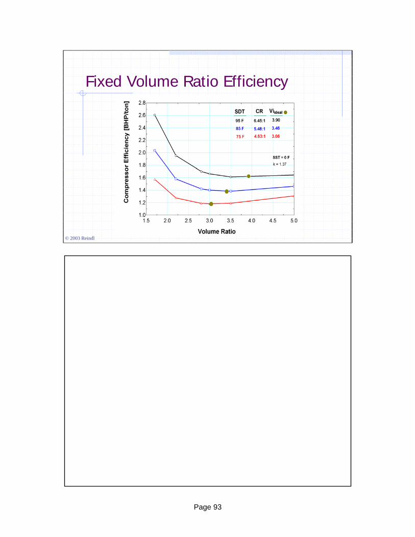
Page 93
© 2003 Reindl
Fixed Volume Ratio Efficiency

Page 94
© 2003 Reindl
Fixed Volume Ratio Efficiency

Page 95
© 2003 Reindl
Fixed Volume Ratio Efficiency

Page 96
© 2003 Reindl
Fixed vs. Variable Volume Ratio

Page 97
© 2003 Reindl
Selection Considerations1. Expected range of operating suction & discharge pressures
a) single stage or two stage operation (booster or high-stage)b) swing duty (boosters operating as a single stage)c) load variability over time (large pull-down loads vs. relatively
constant loads)2. Climate type and system minimum head pressure
constraints3. Oil separator sizing/selection4. Oil cooling methods5. System and package losses for check valves, service
valves, strainers installed around the compressor6. Expected maintenance costs over machine’s life

Page 98
© 2003 Reindl
Fixed Vi Selection Ranges
1.5 – 3.01.5 – 2.71.4 – 2.540
2.0 – 3.51.7 – 3.01.5 – 2.720
3.0 – 4.02.7 – 3.52.5 – 3.50
4.0 – 5.03.5 – 5.03.5 – 5.0-20
5.0 or higher5.0 or higher5.0 or higher-40
Low180 – 135 psig
(95 - 80°F SCT)
Medium180 – 115 psig
(95 – 70°F SCT)
High180 – 100 psig
(95 - 65°F SCT)
Head Pressure Range1
Sat. Suction Temperature[°F]

Page 99
© 2003 Reindl
Frequency Analysis for Madison
0
500
1000
1500
2000
2500
3000
3500
4000
9593918987858381797775737169676563
Saturated Condensing Temperature [F]
Hou
rs p
er Y
ear
Dry OperationWet Operation
Madison, WI

Page 100
© 2003 Reindl
Typical Part-Load Compressor Performance
Source: Manske, K. et al., 2000
Large screw and reciprocating compressors typically have the capability for reducing their capacity to match the required refrigeration demand by the system. Screw compressors typically accomplish this task by the use of a slide valve that, effectively, changes the point where the compression process begins along the axis of the screw. Most screw compressors have the ability to continuously modulate capacity between 10 to 100% of its available full load capacity. Some screw compressors are also equipped with variable speed drives that gives further flexibility to their part-load operation – these are not considered in the following analysis. Reciprocating compressors can be equipped with cylinder unloaders. Unloaders consist of hydraulically or electrically-actuated push rods that hold open suction valves on individual or groups of cylinders. By holding open the suction valves, the number of cylinders that are providing active gas compression is reduced; thereby, reducing the compressor’s capacity. As screw compressors are unloaded, their power and oil cooling requirements decrease, but not necessarily in direct proportion to capacity. Reciprocating compressors tend to unload more linearly. Unloading curves for both the screw and multi-cylinder reciprocating compressors are shown in the figure above. These curves give the fraction of full load power (%FLP) the compressor will require when operated at a specific percent of its full load capacity (%FLC) or part-load ratio. The part-load characteristic for the reciprocating compressor does not pass through the origin of the above figure because of the additional compressor power requirement (approx. 3%) to overcome parasitic losses associated with frictional and windage effects on the unloaded cylinders. The part-load characteristics for both compressors were obtained from thecompressor manufacturer, Vilter. These characteristics are expected to be representative, but the characteristics of compressors from different manufacturers may differ from those above due to different compressor designs and manufacturing processes.Note, the above unloading curve and subsequent analysis does not consider economized operation.

Page 101
© 2003 Reindl
Compressor Part-Load Efficiency Comparison
Source: Manske, K. et al., 2000
If multiple compressors are used to meet the refrigeration load, it is desirable to operate the compressors at the lowest combined power while still meeting the system loads. In refrigeration systems with variable loads, the delivered capacity of the compressors must be modulated by unloading the compressors in order to balance the compressor(s) capacity with the refrigeration demands of the system. Each compressor, depending upon type and manufacturer, may have a different unloading characteristic. The following results are strictly valid only for the particular screw and reciprocating compressors investigated in this study; however, the general concepts can be applied to all refrigeration systems with multiple compressors.A theoretical refrigeration system utilizing two compressors operating in parallel was used to explore optimum compressor operation. Compressor performance can be characterized in terms of specific power, i.e., the dimensionless ratio of the compressor power to refrigeration capacity at a particular set of operating conditions (saturated suction temperature, saturated discharge temperature, and part-load ratio). The specific capacity is the inverse of the coefficient of performance (COP). The figure above shows a performance comparison, in terms of the compressor specific power, between the screw and reciprocating compressors for several different saturated suction temperatures over a range of part-load conditions assuming a fixed saturated discharge temperature of 29.4°C (85°F). Reciprocating compressors unload nearly linearly and their performance curve should, theoretically, be flat for a fixed suction temperature. The slight increasing trend (corresponding to a decrease in compressor performance) from left to right in the figure for the reciprocating compressor is a result of increasing pressure drop in the dry suction line due to increasing refrigerant mass flow rate. The additional (3%) increase in total compressor power discussed above also contributes to the increasing trend in specific power. Several observations can be made about compressor operation from the figure.• A single screw compressor unloaded to 25 percent of its full load capacity has nearly a 50 percent increase in specific power when compared to a reciprocating compressor. • Screw compressors perform better than reciprocating compressors when operated near full load. The performance advantage increases as the suction pressure drops.• Reciprocating compressors are better suited in refrigeration systems where significant unloading, i.e. load following, is required.• From an energy standpoint, is more important to size screw compressors correctly as compared to multi-cylinder reciprocating compressors.

Page 102
© 2003 Reindl
Compressor Part-Load Efficiency
A screw compressor unloaded to 25% of its full load capacity has nearly 50% higher BHP/ton vs. recip.
Multi-cylinder reciprocating compressors unload nearly linearly
Screw compressors perform better than reciprocating compressors when operated near full load
Unloading penalty for screw compressors is greater with increasing pressure lifts

Page 103
© 2003 Reindl
Refrigeration Load Allocation
Assuming we have all screw compressors, how should we distribute or allocate the refrigeration load?

Page 104
© 2003 Reindl
Efficiency of Two Compressor Operation
Source: Manske, K., et al., 2000
The above plot assumes that two 110 ton compressors are available to meet varying proportions of a 220 ton peak refrigeration load. The saturated suction temperature is 0 F and the saturated condensing temperature is 85 F. The part-load characteristics are based on the Vilter single screw.The following can be observed from the above plot. If the total system load is greater than 60% of the full load (0.6*220= 132 tons), it is preferable to fully load one of the compressors and use the other compressor to “load-follow”. If the load is less than 60% of the design full load, it is preferable to equally unload the two compressors. This behavior is dictated by the unloading characteristic of the screw compressor and, in this case, independent of the condensing temperature.

Page 105
© 2003 Reindl
Efficiency of Two Compressor Operation
Source: Manske, K., et al., 2000
Screw compressors unload non-linearly and their parallel operation must be treated quite differently compared to reciprocating compressors. The figure above shows a plot of the aggregate specific power for a system with two equally sized screw compressors operating in parallel. Each separate line on the plot represents a different total system load. The system load is expressed in terms of the system part load ratio (PLR) defined as the ratio of the actual delivered system capacity to the total available capacity of both compressors at full load. Starting at the far right of the plot for a given load, one compressor is fully loaded and the other compressor is operating at part load such that the combined capacity of the two compressors matches the total system load. The abscissa is the ratio of the capacity of the lead (more heavily loaded) compressor to the capacity of lag (less heavily loaded) compressor. By progressing from right to left along a constant system load line, the capacity of the lead compressor is reduced while that for the lag compressor is increased. The figure shows that, for part load ratios below approximately 0.65, optimal operation results when the load is split equally between the two compressors (a compressor capacity ratio of 1). When the system has a part load ratio above 0.65, the system performance is optimized when one compressor is fully loaded and the remaining compressor is loaded to make up the difference. This behavior can be explained by the previously-shown part-load characteristics, which illustrates that the specific power of an individual screw compressor begins to increase very rapidly if it is operated with a compressor part load ratio below 0.5. The values of the aggregate specific power shown above depend on several factors, including the compressor performance characteristics and pressure drop in the compressor suction lines. However, the conclusions relating on how to optimize the combined operation of the two compressors are independent of these factors.

Page 106
© 2003 Reindl
Efficiency of Unequally Sized Compressors
Source: Manske, K., et al., 2000
The above example illustrates how unequally-sized compressors function to meet system loads. At system loads equal to or greater than about 72% of design (209 tons or greater), it is preferable to fully load the larger screw compressor and use the smaller compressor to load-follow. As the system load continues to drop below 72%, it is advantageous to fully load the smaller compressor and begin unloading the larger; however, if the system load drops below about 58% (197 tons) both screw compressors should operate at equal part-load ratios.

Page 107
© 2003 Reindl
Variable Speed Screw Compressor
0 0.1 0.2 0.3 0.4 0.5 0.6 0.7 0.8 0.9 110
15
20
25
30
35
40
45
50
55
Part-Load Ratio
Com
pres
sor P
ower
[kW
E]
Fixed Speed
Variable Speed
FES 315S Booster Compressor
CF Industries
Albany Terminal
Compressor C-2
Fixed Vi=2.6
July 17, 2003
kw=9.55645 + 15.576·PLRCalculated + 26.2308·PLRCalculated2kw=9.55645 + 15.576·PLRCalculated + 26.2308·PLRCalculated2
kw=22.5113 + 11.5401·PLRCalculated + 16.0278·PLRCalculated2kw=22.5113 + 11.5401·PLRCalculated + 16.0278·PLRCalculated2

Page 108
© 2003 Reindl
Compressor Operation Conclusions
When screws & recips are used, unload recipfirst and screw last
Always try to operate screw compressors at part-load ratios greater than 50%
Remember operating systems with unequal sized compressors differs from systems with equally sized compressors
Compressors in industrial refrigeration systems regularly operate at part-load conditions. Part-load compressor operation is required in order to balance the refrigeration capacity of the compressors with the refrigeration demand from the system. Reciprocating compressors have near-linear unloading curves and therefore introduce relatively small performance penalties when operated at low part-load ratios. This is not the case however for screw compressors. As screw compressors are unloaded they require more power per unit of cooling capacity. It is recommended that screw compressors be sized appropriately so they can be operated at or near full capacity as much as possible. Screw compressors should be used for base loading and reciprocating compressors should be used to meet the transient portion of a varying load.If two screw compressors are sharing a load, there exists a point where it is better to fully load one compressor rather than split the load equally. In the case of two equally sized screw compressors, the optimal situation occurs when the compressors share the load up to an identifiable crossover point which occurs when the load on the system is about 66 percent of the combined available capacity of the compressors. At loads above that point it is best to fully load one of the screws and make up the difference with the other. The crossover point is a characteristic of type and size of compressors used. When load sharing between two unequal sized screw compressors is required, it is best to first fully load the smaller of the two, then at a certain identifiable crossover point, fully load the larger of the two compressors and make up the difference with the smaller of the two. Calculations with unequal sized screw compressors (the larger compressor has 64% greater capacity compared to the smaller compressor), indicated that this cross-over point occurred when the load was 76 percent of the available capacity of both compressors. Crossover points are independent of compressor suction and discharge conditions.

Page 109
© 2003 Reindl
Intercooler Pressure Reset
109

Page 110
© 2003 Reindl
Intercooler Pressure Reset
How do we determine intercooler pressure?requirements of “high” temperature loadsequal compression ratio on boosters and high stage machinesdesigner’s selection of intermediate temperatureother strategies

Page 111
© 2003 Reindl
Determining Intermediate Temperature
A commonly applied rule-of-thumb for approximating an optimum intermediate pressure level is given by:
P P Pint cond evap= ⋅
where all pressures are expressed as absolute pressures
Pint = Intercooler pressure (psia)Pcond = Condensing pressure (psia)Pevap = Low temperature evaporator pressure (psia)
Keep in mind that the pressures in the above relationship need to be in absolute terms. Recall the conversion between absolute and gage pressures:
Pabs = Pgage + Patm
Where Patm is the local atmospheric pressure (14.7 psi at sea level).

Page 112
© 2003 Reindl
Determining Intermediate Pressure
As head pressure floats, the optimum intermediate pressure changes
Many systems establish their interstage pressure and leave it fixed
this strategy can lead to significant energy penalties on an annual basis
alternative strategies aim to reset the intermediate pressure
The previous relationship is an approximation, how good is it?

Page 113
© 2003 Reindl
Case Study
Anhydrous ammonia storage terminal
system charge – 30,000 tonslow stage pressure ~0.5 psig – critical control ptintermediate stage pressure: 55 psiga total of 560 HP of compressors
G

Page 114
© 2003 Reindl
EvaporativeCondenserEvaporativeCondenser
High StageCompressors
IntercoolerLow Stage
Compressor
EvaporativeCondenserEvaporativeCondenser
To Purge
Hi Press. RecHi Press. Rec
KO Drum
BC-1 BC-2 BC-3
82 kW heater
Two Stage Compression with Single Temperature Level
DTR, 8/27/00
HS-1 HS-2 HS-3

Page 115
© 2003 Reindl
Intercooler Pressure
35 40 45 50 55 60 65 70 75 8040
42
44
46
48
50
Intercooler Pressure [psia]
Syst
em P
ower
[hp]
Pcond=125 psig
Pcond = 150 psig
Pcond = 175 psig
The above plot illustrates the optimum interstage pressure for the two-stage compression single temperature level system. The curves illustrate the total system horsepower requirements as the intercooler pressure is reset in a range from 40 – 80 psia based on a relatively simple mathematical model of the system. The model of this particular system neglects piping pressure drops (piping pressure drop effects will influence the optimum interstage pressure as will be illustrated in the section on single stage vs. two stage). Each curve in the above plot represents a fixed condensing pressure range from 125 psig to 175 psig. The solid
dots show the points of optimum intercooler pressure as estimated by the square root relationship previously presented. As is apparent, the square root relationship provides good estimates of the true optimum. Note that the best operating strategy involves resetting the intercooler pressure as head pressure changes.

Page 116
© 2003 Reindl
The Need for Multi-Stage SystemsHigh compression ratios
recip compressor limits: ~8:1
screw compressor limits: ~18:1
High fixed head pressures
floating head pressure decreases the attractiveness of multi-stage systems
Loads at multiple temperature levels
As we operate systems at lower and lower suction pressures (to achieve lower temperature operation), we eventually reach limits of the compression devices in our systems. Reciprocating compressors have a compression ratio limit of approximately 8:1 which means that if our design condensing temperature was 196 psia (95 F), our lowest possible evaporator pressure/temperature for a single stage system would be 24.5 psia (about –8.5 F). In the case that our application required colder temperatures, staging would be required.It is widely stated that the two stage system is more efficient than a single stage system. Although this is true in a number of circumstances, its applicability needs to be carefully evaluated for the application and control setpoints in a proposed or actual system. The question is: when does 2-stage make sense (from an energy efficiency standpoint)? The corollary to this question is: When should I operate a two stage system as a single stage? This is what we would call a “swing” system.

Page 117
© 2003 Reindl
Case Study: -10 F System
65 70 75 80 85 90 95 100-10.0
-8.0
-6.0
-4.0
-2.0
0.0
2.0
4.0
6.0
8.0
10.0
Minimum Saturated Condensing Temperature Allowed [°F]
Perc
ent S
avin
gs o
f Com
pres
sor H
orse
pow
er
Actual Simulation ResultsActual Simulation Resultsov
er S
ingl
e-St
age
Com
pres
sion High-Stage - Recip.
Low-Stage - Screw
Two-staging will save on compressorpower above a temp. of 80°F.
Source: Manske, K., 2000
We considered the operation of a two stage system with a low stage suction temperature of –10 F (pretty much on the edge if we were to use recips for a single stage application). The above plot represents a system that uses screw compressors as the boosters and recip compressors for the high stage. The low stage suction pressure is fixed at -10 F with the intermediate stage temperature fixed at 23 F. Interestingly, at minimum saturated condensing temperature below 80 F, a two stage system will consume more energy than a single stage system. This is due to a few contributing factors.
1. The second stage includes additional piping that imposes suction line pressure drops (approximately twice the aggregate pressure drop as compared to a single stage system).
2. The above system has a fixed intermediate temperature that will not be optimum as the condensing temperature changes over the course of the year.

Page 118
© 2003 Reindl
Case Study: -10 F System
Source: Manske, K., 2000
65 70 75 80 85 90 95-15
-10
-5
0
5
10
15
20
Saturated Condensing Temperature [°F]Perc
ent S
avin
gs o
f Com
pres
sor H
orse
pow
er
2 stage screw s w ith idealintermediate temperature
2 stage screw s w ith 23°Fintermediate temperature
50% part load
full load
full loadpart load
2 stage reciprocating compressors
ideal int. temperature23°F int. temperature
economizer screw s
-10°F Suction Temp.over
Sin
gle
Stag
e C
ompr
essi
on
The above plot shows the percent savings of various two-stage refrigeration system options over a single stage system at full load (upper set of curves) and ½ load (lower set of curves). The two cases for each load represent each a fixed intermediate temperature level of 23 F and a floating intermediate temperature level which minimizes the system power required.The lower set of lines in the above plot shows that two stage systems using screw compressors have a much higher saturated condensing temperature at which a two stage system becomes competitive as compared to a system using recipcompressors (the upper set of lines). Also included in each of the cases are a fixed intermediate temperature (23 F) and an optimized intermediate temperature (pressure).

Page 119
© 2003 Reindl
Intermediate Temperature
Source: Manske, K., 2000
Selecting intermediate pressures other than the optimum will reduce the effectiveness of a two-stage compression system. The penalty of using a non-ideal intermediate pressure is most significant with screw compressors. This effect can best be explained with the help of the above figure. The figure shows the saturation temperature that the intermediate pressure receiver should operate at to minimize the compressor horsepower per ton for the composite two-stage system. The optimum intermediate pressure was found using optimization routines in a simulation environment. Curves are shown for both single screw and reciprocating compressors. It is interesting to note that the optimized temperatures for the screw and reciprocating compressor systems straddle the “rule of thumb" ideal intermediate suggested by Mitchell and Braun, 1998.

Page 120
© 2003 Reindl
Multi-Stage System Conclusions
Only consider multi-stage for system temps below 0 F [-17.8 C]
Use care in selecting intermediate temperature level (reset if possible)
Systems with floating head pressure erode advantages of multi-stage systems
(practically speaking, below -28 F, -33 C)

Page 121
© 2003 Reindl
Next StepsNext StepsNext Steps

Page 122
© 2003 Reindl
What are the steps?1. baseline system performance2. compare baseline with benchmarks (competitors, published, …)3. identify potential opportunities4. estimate impact/benefit to system5. estimate capital cost6. assess operational risks/constraints7. prioritize by greatest benefit to cost8. follow-up and quantify benefit & continuously improve
Establish Goals for Efficiency Improvement

Page 123
© 2003 Reindl
Baseline system performance
Identify potential energyefficiency improvements
Estimate impact/benefit to system
Assess operational risks
Operational riskscriteria satisfied?
Does performance exceed benchmarks?
yes
no
Does performance exceed benchmarks?
yes
no
Economic criteriaSatisfied?
yes
noEconomic criteriaSatisfied?
yes
no
Implement and follow-up with next opportunity
no
yes

Page 124
© 2003 Reindl
Energy Efficiency Measures
Approaches for efficiency improvementsfloating head pressure control
demand-shifting strategies
defrosting
compressor operation/sizing
multi-stage systems
maintenance issues

Page 125
© 2003 Reindl
Achieving Energy Conservation
Opportune times to evaluate systemin conjunction with proposed expansions
bi-annually or on a set schedule
upgrades (as part of management-of-change)
Choose ECM projects that offer good cost/benefit and low risk

Page 126
© 2003 Reindl
Validation/Verification
Compare post-ECM system performance with pre-ECM system performance
use normalization to account for differences inweather
production
compare with estimated impact from feasibility assessment(s)
is the trend “as-expected”
is the magnitude of the impact “as-anticipated”

Page 127
© 2003 Reindl
How & When
Don’t try to do everything at oncemake changes slowly and incrementally to minimize risk to system operationbe sure to involve safety, operations, mechanics, and production personnel in proposed system changesinclude changes in your management-of-change (MOC) procedures as required by your plant’s process safety management (PSM) programtraining, training, and training

Page 128
© 2003 Reindl
It takes effort!
Baseline, implement, & verifystrive for continuous efficiency
improvements

Page 129
© 2003 Reindl
Good Luck!
Innovation – Knowledge – Progress
www.irc.wisc.edu