enhancement of granulation and start-up in the anaerobic
TRANSCRIPT

Retrospective Theses and Dissertations Iowa State University Capstones, Theses andDissertations
1994
Enhancement of granulation and start-up in theanaerobic sequencing batch reactorRandall Anthony WirtzIowa State University
Follow this and additional works at: https://lib.dr.iastate.edu/rtd
Part of the Chemical Engineering Commons, and the Civil Engineering Commons
This Dissertation is brought to you for free and open access by the Iowa State University Capstones, Theses and Dissertations at Iowa State UniversityDigital Repository. It has been accepted for inclusion in Retrospective Theses and Dissertations by an authorized administrator of Iowa State UniversityDigital Repository. For more information, please contact [email protected].
Recommended CitationWirtz, Randall Anthony, "Enhancement of granulation and start-up in the anaerobic sequencing batch reactor " (1994). RetrospectiveTheses and Dissertations. 10523.https://lib.dr.iastate.edu/rtd/10523

INFORMATION TO USERS
This manuscript has been reproduced from the microfilm master. UMI
fihns the text directly from the original or copy submitted. Thus, some
thesis and dissertation copies are in typewriter face, while others may
be fi-om any type of computer printer.
The quality of this reproduction is dependent upon the quality of the copy submitted. Broken or indistinct print, colored or poor quality
illustrations and photographs, print bleedthrough, substandard margins, and improper alignment can adversely affect reproduction.
In the unlikely event that the author did not send UMI a complete
manuscript and there are missing pages, these will be noted. Also, if
unauthorized copyright material had to be removed, a note will indicate the deletion.
Oversize materials (e.g., maps, drawings, charts) are reproduced by
sectioning the original, beginning at the upper left-hand corner and
continuing from left to right in equal sections with small overlaps. Each
original is also photographed in one exposure and is included in
reduced form at the back of the book.
Photographs included in the original manuscript have been reproduced
xerographically in this copy. Higher quality 6" x 9" black and white
photographic prints are available for any photographs or illustrations
appearing in this copy for an additional charge. Contact UMI directly to order.
University Microfilms International A Bell & Howell Information Company
300 North Zeeb Road. Ann Arbor, Ml 48106-1346 USA 313/761-4700 800/521-0600

Order Number 9503608
Enhancement of granulation and start-up in the anaerobic sequencing batch reactor
Wirtz, Randall Anthony, Ph.D.
Iowa State University, 1994
U M I 300 N. ZeebRd. Ann Arbor, MI 48106


Enhancement of granulation and start-up in the
anaerobic sequencing batch reactor
by
Randall Anthony Wirtz
A Dissertation Submitted to the
Graduate Faculty in Partial Fulfillment of the
Requirements for the Degree of
DOCTOR OF PHILOSOPHY
Department: Civil and Construction Engineering Major: Civil Engineering (Environmental Engineering)
For the Mijor Department
For the Graduate College
Iowa State University Ames, Iowa
1994
Signature was redacted for privacy.
Signature was redacted for privacy.
Signature was redacted for privacy.

ii
To Kalla Kaye: thank you for your love, support, encouragement, and patience.

iii
TABLE OF CONTENTS
Page
LIST OF TABLES vii
LIST OF FIGURES xii
LIST OF ABBREVIATIONS xvii
ACKNOWLEDGEMENTS xx
INTRODUCTION 1 Background I Objectives and Scope 3
LITERATURE REVIEW 6 Origins of Life 6 Historical Perspectives of Anaerobic Bacteria 7 The Anaerobic Bacteria 10
Anaerobes and Oxygen 11 Physiology of Anaerobes 14 Hydrolytic/Fermentative Bacteria 17 Acetogenic Bacteria 20
Acetogenic Dehydrogenations 21 Acetogenic Hydrogenations 23
Methanogenic Bacteria 25 General Background 25 Biochemistry of Methanogens 28
Interplay among the Anaerobic Bacteria 41 Anaerobic Wastewater Treatment 44
Anaerobic versus Aerobic Treatment 44 Environmental/Operational Parameters in Anaerobic Treatment 46
Environmental Parameters 47 Operational Parameters 54
Early Research 58 High-Rate Anaerobic Treatment 60
The Anaerobic Contact Process 60 The Anaerobic Filter 61 The Hybrid Anaerobic Filter 64 The Expanded-Bed Anaerobic Reactor 65

iv
The Upflow Anaerobic Sludge Blanket Reactor 68 The Anaerobic Sequencing Batch Reactor 70
The Phenomenon of Granulation 81 Theory of Bacterial Adhesion and Aggregation 81 General Characteristics of Granules in Anaerobic Systems 83 Granulation in the ASBR 85
First Report of Granulation 85 Further Studies with Granular Biomass in the ASBR 87
Granulation in the UASB and Expanded-Bed Processes 89 Granule Microbiology and Morphology 90 Granule Chemical Composition 95 Activity of Granular Biomass 97 Modeling the Granulation Process 100 Effect of Substrate and Temperature 104 Effect of Chemical Enhancement 106 Effect of Physical Enhancement 113
EXPERIMENTAL SETUP 115 Anaerobic Sequencing Batch Reactor Design 115 Gas/Foam Separation System 118 Biogas Recirculation System 119 Biogas Collection and Measurement System 121 Substrate Feed and Effluent Decant Systems 123 Coagulant Feed System 124
EXPERIMENTAL PROCEDURES 125 Substrate Feed Preparation 125 Biological Seeding of the ASBR 130 ASBR Start-up and Operation 132 ASBR Mixing 135 Granulation Enhancement 136
Attachment Matrices 136 Coagulant Addition 138
EXPERIMENTAL TESTING 141 Chemical Oxygen Demand 142 Volatile Fatty Acids 145 Effluent Suspended Solids 147 Mixed Liquor Suspended Solids 149 Hydrogen Ion Concentration 151 Alkalinity 151

V
Ammonia Concentration 153 Biogas Production and Composition 155 Automated Image Analysis 159 Specific Methanogenic Activity 160 Scanning and Transmission Electron Microscopy 163 Elemental Analysis of Biomass 164
RESULTS AND DISCUSSION 166 Sucrose Experiments 167
Control Study 167 Operational Performance 168 Solids and Granulation 170
Powdered Activated Carbon Enhancement Study 175 Operational Performance 175 Solids and Granulation 179 PAC Effect 181
Granular Activated Carbon Enhancement Study 181 Operational Performance 182 Solids and Granulation 185 GAC Effect 185
Garnet Enhancement Study " 187 Operational Performance 187 Solids and Granulation 191 Garnet Effect 193
Silica Sand Enhancement Study 193 Cationic Polymer Enhancement Smdy 194
Operational Performance 198 Solids and Granulation 202 Cationic Polymer Effect 203
PolyDADM Enhancement Study 206 Operational Performance 206 Solids and Granulation 210 PolyDADM Effect 212
Ferric Chloride Enhancement Study 213 Operational Performance 213 Solids and Granulation 215 Ferric Chloride Effect 218
Beef/Glucose Experiments 218 Control Study 219
Operational Performance 219 Solids and Granulation 221

vi
Cationic Polymer Enhancement Study 225 Operational Performance 225 Solids and Granulation 228 Cationic Polymer Effect 231
Sunmiary of Enhancement Results 231 Specific Methanogenic Activity Experiments 234
Background and Theory 234 Specific Methanogenic Activity Results 237
Sucrose Tests 237 Acetate Tests 239
Electron Microscopy 242 Granule Surface 243 Granule Structure and Arrangement 249
Granule Elemental Analysis 254
CONCLUSIONS AND RECOMMENDATIONS 256
APPLICATIONS 261 Background 261 Economics 261
Cationic Polymer 262 PAC and GAC 263
REFERENCES 266
APPENDIX: EXPERIMENTAL DATA TABLES 285

vii
LIST OF TABLES
Page
Table 1. Examples of anaerobic respiration. 16
Table 2. Proton-reducing reactions by the acetogenic bacteria [14, 27, 143, 168]. 23
Table 3. The methanogenic bacteria [12], 26
Table 4. Methanogenic substrates [12]. 27
Table 5. Important reactions by the methanogens [12, 168]. 27
Table 6. Effects of alkali and alkaline-earth metals on anaerobic digestion [95]. 52
Table 7. Bacterial counts in granules from UASB reactors [31, 33]. 91
Table 8. General composition of granules [31]. 96
Table 9. Granule chemical composition [32, 33], 96
Table 10. Specific methanogenic activity of various biomass [32, 87]. 99
Table 11. Substrates suitable for granule formation. 105
Table 12. Solubility products of metal salts [98]. 111
Table 13. Sucrose feed mixture. 126
Table 14. Beef extract and glucose feed mixture. 127
Table 15. Composition of the beef extract soup base. 128
Table 16. Nutrient (NPK) solution. 128
Table 17. Trace metal solution. 129
Table 18. Ames municipal water analysis. 131
Table 19. ASBR cycle time for 48 and 24-hr HRTs. 133

viii
Table 20. Attachment matrices utilized for granulation enhancement. 138
Table 21. Polymer characteristics. 139
Table 22. Coagulants utilized for granulation enhancement. 139
Table 23. Operational parameters routinely tested. 141
Table 24. Reagents used in the COD test. 144
Table 25. Gas chromatography analysis setup. 158
Table 26. Elemental analysis of granules. 165
Table 27. Start-up and granulation summary. 232
Table 28. Summary of specific methanogenic activity experiments. 238
Table 29. Chemical composition of granular and initial seed biomass. 255
Table 30. COD data for the sucrose control test. 286
Table 31. Biogas data for the sucrose control test. 287
Table 32. Volatile acids data for the sucrose control test. 291
Table 33. Particle size analysis for the sucrose control test. 291
Table 34. Alkalinity and pH data for the sucrose control test. 292
Table 35. Solids data for the sucrose control test. 293
Table 36. COD data for the sucrose+PAC test. 294
Table 37. Biogas data for the sucrose+PAC test. 296
Table 38. Volatile acids data for the sucrose+PAC test. 303
Table 39. Particle size analysis for the sucrose-l-PAC test. 304
Table 40. Alkalinity and pH data for the sucrose+PAC test. 305

307
309
310
315
315
316
317
318
319
323
323
324
325
326
327
329
329
330
331
332
336
ix
Solids data for the sucrose+PAC test.
COD data for the sucrose+GAC test.
Biogas data for the sucrose+GAC test.
Volatile acids data for the sucrose+GAC test.
Particle size analysis for the sucrose+GAC test.
Alkalinity and pH data for the sucrose+GAC test.
Solids data for the sucrose+GAC test.
COD data for the sucrose+garnet test.
Biogas data for the sucrose+garnet test.
Volatile acids data for the sucrose+gamet test.
Particle size analysis for the sucrose+garnet test.
Alkalinity and pH data for the sucrose+garnet test.
Solids data for the sucrose+garnet test.
COD data for the sucrose+sand test.
Biogas data for the sucrose+sand test.
Volatile acids data for the sucrose+sand test.
Alkalinity and pH data for the sucrose+sand test.
Solids data for the sucrose+sand test.
COD data for the sucrose+cationic polymer test.
Biogas data for the sucrose+cationic polymer test.
Volatile acids data for the sucrose+cationic polymer test.

X
Table 62. Particle size analysis for the sucrose+cationic polymer test. 336
Table 63. Alkalinity and pH data for the sucrose+cationic polymer test. 337
Table 64. Solids data for the sucrose+cationic polymer test. 338
Table 65. COD data for the sucrose+polyDADM test. 339
Table 66. Biogas data for the sucrose+polyDADM test. 340
Table 67. Volatile acids data for the sucrose+polyDADM test. 344
Table 68. Particle size analysis for the sucrose+polyDADM test. 344
Table 69. Alkalinity and pH data for the sucrose+polyDADM test. 345
Table 70. Solids data for the sucrose+polyDADM test. 346
Table 71. COD data for the sucrose+ferric chloride test. 347
Table 72. Biogas data for the sucrose+ferric chloride test. 348
Table 73. Volatile acids data for the sucrose+ferric chloride test. 350
Table 74. Particle size analysis for the sucrose+ferric chloride test. 350
Table 75. Alkalinity and pH data for the sucrose+ferric chloride test. 350
Table 76. Solids data for the sucrose+ferric chloride test. 351
Table 77. COD data for the beef/glucose control test. 352
Table 78. Biogas data for the beef/glucose control test. 353
Table 79. Volatile acids data for the beef/glucose control test. 356
Table 80. Particle size analysis for the beef/glucose control test. 356
Table 81. Alkalinity and pH data for the beef/glucose control test. 357
Table 82. Solids data for the beef/glucose control test. 358

xi
Table 83. COD data for the beef/glucose control test. 359
Table 84. Biogas data for the beef/glucose control test. 360
Table 85. Volatile acids data for the beef/glucose control test. 363
Table 86. Particle size analysis for the beef/glucose control test. 363
Table 87. Alkalinity and pH data for the beef/glucose control test. 364
Table 88. Solids data for the beef/glucose control test. 365
Table 89. SMA test with the PAC-enhanced ASBR, day 158. 366
Table 90. SMA test with the PAC-enhanced ASBR, day 169. 369
Table 91. SMA test with the PAC-enhanced ASBR, day 228. 373
Table 92. SMA test with the PAC-enhanced ASBR, day 283. 375
Table 93. SMA test with the GAC-enhanced ASBR, day 65. 377
Table 94. SMA test with the GAC-enhanced ASBR, day 76. 380
Table 95. SMA test with the GAC-enhanced ASBR, day 93. 383
Table 96. SMA test with the GAC-enhanced ASBR, day 113. 385
Table 97. SMA test with the GAC-enhanced ASBR, day 135. 387
Table 98. SMA test with the GAC-enhanced ASBR, day 190. 389
Table 99. SMA test with the GAC-enhanced ASBR, day 195. 391
Table 100. SMA test with the garnet-enhanced ASBR, day 83. 393

xii
LIST OF FIGURES
Page
Figure 1. Simplified pathways for polysaccharide fermentation by the acidogenic bacteria [14]. 18
Figure 2. Biochemistry of carbon dioxide utilization by methanogens. 34
Figures. Biochemistry of methyl compound utilization by methanogens. 35
Figure 4. Biochemistry of acetate utilization by methanogens. 36
Figure 5. Substrate and intermediate product flow among anaerobic bacteria. 42
Figure 6. The anaerobic contact process. 61
Figure 7. The anaerobic filter. 62
Figure 8. The hybrid anaerobic filter. 65
Figure 9. The anaerobic expanded-bed (fluidized-bed) reactor. 66
Figure 10. The upfiow anaerobic sludge blanket reactor. 69
Figure 11. The anaerobic sequencing batch reactor. 71
Figure 12. The phases of the anaerobic sequencing batch reactor. 72
Figure 13. Graphical representation of the Monod function. 74
Figure 14. Theoretical substrate concentration and F/M ratio over time in the ASBR. 75
Figure 15. Anaerobic sequencing batch reactor setup. 116
Figure 16. Schematic of the top cover of the ASBR. 117
Figure 17. ASBR biogas recirculation diffiiser system. 120
Figure 18. COD removal for the sucrose control study. 169

xiii
Figure 19. Methane production for the sucrose control study. 169
Figure 20. Volatile acids data for the sucrose control study. 171
Figure 21. Alkalinity and pH data for the sucrose control study. 171
Figure 22. MLSS and SRT for the sucrose control study. 173
Figure 23. Average particle size data for the sucrose control study. 173
Figure 24. COD removal for the PAC-enhanced sucrose study. 177
Figure 25. Methane production for the PAC-enhanced sucrose study. 177
Figure 26. Volatile acids data for the PAC-enhanced sucrose study. 178
Figure 27. Alkalinity and pH data for the PAC-enhanced sucrose study. 178
Figure 28. MLSS and SRT for the PAC-enhanced sucrose study. 180
Figure 29. Average particle size data for the PAC-enhanced sucrose study. 180
Figure 30. COD removal for the GAC-enhanced sucrose study. 183
Figure 31. Methane production for the GAC-enhanced sucrose study. 183
Figure 32. Volatile acids data for the GAC-enhanced sucrose study. 184
Figure 33. Alkalinity and pH data for the GAC-enhanced sucrose study. 184
Figure 34. MLSS and SRT for the GAC-enhanced sucrose study. 186
Figure 35. Average particle size data for the GAC-enhanced sucrose study. 186
Figure 36. COD removal for the garnet-enhanced sucrose study. 189
Figure 37. Methane production for the garnet-enhanced sucrose study. 189
Figure 38. Volatile acids data for the garnet-enhanced sucrose study. 190
Figure 39. Alkalinity and pH data for the garnet-enhanced sucrose study. 190

xiv
Figure 40. MLSS and SRT for the garnet-enhanced sucrose study. 192
Figure 41. Average particle size data for the garnet-enhanced sucrose study. 192
Figure 42. COD removal for the silica sand-enhanced sucrose study. 195
Figure 43. Methane production for the silica sand-enhanced sucrose study. 195
Figure 44. Volatile acids data for the silica sand-enhanced sucrose study. 196
Figure 45. Alkalinity and pH data for the silica sand-enhanced sucrose study. 196
Figure 46. MLSS and SRT for the silica sand-enhanced sucrose study. 197
Figure 47. COD removal for the cationic polymer-enhanced sucrose study. 199
Figure 48. Methane production for the cationic polymer-enhanced sucrose study. 199
Figure 49. Volatile acids data for the cationic polymer-enhanced sucrose study. 200
Figure 50. Alkalinity and pH data for the cationic polymer-enhance sucrose study. 200
Figure 51. MLSS and SRT for the cationic polymer-enhanced sucrose study. 204
Figure 52. Average particle size data for the cationic polymer-enhanced sucrose study. 204
Figure 53. COD removal for the polyDADM-enhanced sucrose study. 207
Figure 54. Methane production for the poly DADM-enhanced sucrose study. 207
Figure 55. Volatile acids data for the polyDADM-enhanced sucrose study. 208
Figure 56. Alkalinity and pH data for the polyDADM-enhanced sucrose study. 208
Figure 57. MLSS and SRT for the polyDADM-enhanced sucrose study. 211
Figure 58. Average particle size data for the polyDADM-enhanced sucrose study. 211
Figure 59. COD removal for the ferric chloride-enhanced sucrose study. 214

XV
Figure 60. Metliane production for the ferric chloride-enhanced sucrose study. 214
Figure 61. Volatile acids data for the ferric chloride-enhanced sucrose study. 216
Figure 62. Alkalinity and pH data for the ferric chloride-enhanced sucrose study. 216
Figure 63. MLSS and SRT for the ferric chloride-enhanced sucrose study. 217
Figure 64. Average particle size data for the ferric chloride-enhanced sucrose study. 217
Figure 65. COD removal for the beef/glucose control study. 220
Figure 66. Methane production for the beef/glucose control study. 220
Figure 67. Volatile acids data for the beef/glucose control study. 222
Figure 68. Alkalinity and pH data for the beef/glucose control study. 222
Figure 69. MLSS and SRT for the beef/glucose control study. 223
Figure 70. Average particle size data for the beef/glucose control study. 223
Figure 71. COD removal for the cationic polymer-enhanced beef/glucose study. 226
Figure 72. Methane production for the cationic polymer-enhanced beef/glucose study. 226
Figure 73. Volatile acids data for the cationic polymer-enhanced beef/glucose study. 227
Figure 74. Alkalinity and pH data for the cationic polymer-enhanced beef/glucose study. 227
Figure 75. MLSS and SRT for the cationic polymer-enhanced beef/glucose study. 229
Figure 76. Average particle size data for the cationic polymer-enhanced beef/glucose study. 229
Figure 77. Idealized granule exhibiting a layered structure. 235

xvi
Figure 78. Idealized granule exhibiting a non-layered structure. 235
Figure 79. SMA over the course of the GAC enhanced study. 240
Figure 80. SMA comparison of granular and non-granular biomass. 240
Figure 81. SMA comparison of GAC granules fed acetate and sucrose. 241
Figure 82. SEM images of granule surface. 245
Figure 83. SEM images of granule surface. 248
Figure 84. Images of granule interior. 252

XVll
LIST OF ABBREVIATIONS
AIA automated image analysis
ALK alkalinity (bicarbonate)
B boron
BOD biochemical oxygen demand
BOD5 five-day biochemical oxygen demand
BODu ultimate biochemical oxygen demand
Ca calcium
COD chemical oxygen demand
cm centimeters
Cu copper
°C degrees Celsius
FAS ferrous ammonium sulfate
Fe iron
ft feet
g gram
gal gallon
GC gas chromatography
g/L/day grams per liter per day
hr hour

xviii
hrs hours
HRT hydraulic retention time
in inch or inches
k specific substrate removal rate
kn, maximum specific substrate removal rate
K potassium
half saturation constant
Kg solubility product
kg kilogram
L liter
lb pound
m meters
M biomass concentration
Mg magnesium
mgal million gallons
mgd million gallons per day
mg/L milligram per liter
min minute
mL milliliter
MLSS mixed liquor suspended solids
mm millimeters

xix
mol mole or moles
Na sodium
Ni nickel
OLR organic loading rate
P phosphorous
S sulfur or sulfide
SEM scanning electron microscopy
SRT solids retention time
SS suspended solids
STP standard temperature and pressure
TEM transition electron microscopy
TKN total Kjeldahl nitrogen
TOC total organic carbon
TS total solids
TSS total suspended solids
VA volatile acids
VFA volatile fatty acids
vs volatile solids
vss volatile suspended solids
Zn zinc
specific biomass growth rate or 10

XX
ACKNOWLEDGMENTS
The author wishes to express his sincere thanks and appreciation to the many
individuals who had a part in this research. The list of course begins with my major
professor, Dr. Richard R. Dague. Dr. Dague provided knowledge, guidance and
assistance (not to mention the ftinding) throughout this research and served as an extremely
positive role model for all of the graduate students that worked for him. He is a credit to
his profession.
The graduate committee members also are to be thanked for their time and their
input into this research. The members are Dr. T. A1 Austin, CCE; Dr. LaDon C. Jones,
CCE; Dr. Robert E. Andrews, MIPM; and Dr. James A. Thomas, B&B. A special note
of thanks also goes out to Dr. Say-Kee Ong, who filled in for Dr. Jones for the final
dissertation defense.
The author would also like to thank the secretaries of the Civil and Construction
Engineering Department. Without their dedication little would get accomplished in a
reasonable amount of time.
The Analytical Laboratory Service and the Bessey Microscopy Facility at Iowa
State University performed much of the technical and analytical work for this research.
Thank you for your service, promptness, and professional insight.
Finally, the author would like to thank the U.S. Department of Agriculture for their
financial support of this research through the Iowa Biotechnology Byproducts Consortium.

1
INTRODUCTION
Background
High-rate anaerobic wastewater treatment has been practiced in varying degrees for
approximately forty years. The first systems were developed in the 1950s and were
suspended-growth reactors with sludge recycle to maintain the solids retention time (SRT)
independent of the liquid detention time. Attached-growth reactors were developed in the
1960s and maintained long SRTs by physically holding the biomass inside the reactor with
rock or plastic media. Several variations of these systems were developed in the 1970s and
1980s and are described later in this document. One of the most recent developments in
high-rate anaerobic waste treatment is the anaerobic sequencing batch reactor (ASBR),
developed by Richard R. Dague and graduate smdents at Iowa State University.
A U.S. Patent (No. 5,185,079) for the ASBR was issued in February of 1993.
Initial experiments with the ASBR were conducted in 1989 and 1990 by Habben
[47] and Pidaparti [113]. Since that time, the ASBR has been applied at laboratory scale to
several different wastewaters, including starch wastewaters, furfuraldehyde wastewaters,
landfill leachate, and swine wastes. Additionally, fundamental research has been
conducted on a number of operational aspects of the ASBR. Past research has been aimed
at defining appropriate height to width ratios, mixing requirements, and operating
temperatures. Further details concerning ASBR research is found in the literature review
section of this document. The ASBR has also been demonstrated at pilot-scale for a starch
wastewater. A full-scale ASBR for treating swine waste is in the design phase.

Traditionally, one of the most significant problems with anaerobic processes has
been start-up. The systems have normally taken several months (sometimes years) to reach
stable operation at their design conditions. This has been one of the biggest deterrents to
using anaerobic treatment processes at full-scale. Industries, with little knowledge of
anaerobic systems, felt that the systems were slow and took a long time to treat wastes to
the desired degree. What was really the case, however, was that the microbes were "slow
growing," which is not equivalent to "slow working." Although anaerobic systems may
require relatively long start-up times due to their slow growth, once a sufficient consortia
of bacteria has been established, the specific removal rates (per unit biomass) are
comparable to those of aerobic systems.
Because of the requirement for long start-up periods before design load could be
realized in anaerobic systems (including the ASBR), it was decided to study methods of
operation that would decrease the start-up period. By decreasing the start-up time,
industry may be more apt to consider anaerobic treatment systems for their wastewater,
since most industries do not want to wait a half year or longer to have a treatment system
be effective.
It was also decided to study the phenomenon of granulation in the ASBR, which
was first observed by Sung and Dague [142] in a previous study. Granulation is the
agglomeration of individual biomass particles into discrete pellets, or granules, some of
which may grow to 5 or 6 mm in diameter. Granular biomass has several distinct
advantages over flocculent (dispersed) biomass, which will be detailed later. The
3
important point is that the development of a granular biomass is beneficial to the treatment
system, and the earlier it is developed the better. It was expected that optimum conditions
for these two objectives, a short start-up period and the formation of granules, would be
identical. That is, when granulation developed, the system would be mature and able to
handle higher chemical oxygen demand (COD) loading rates. Conversely, when the
system became mature enough to handle higher loading rates, it would be in the process of
granulation. These statements were hypotheses, and definitely not absolute. Therefore, it
was decided to study these phenomena in some detail.
Objectives and Scope
The selected topic for study was a fairly broad, ill-defined area for two main
reasons: (1) there are many factors which contribute to the start-up efficiency and
granulation of biomass in anaerobic reactors, and (2) granulation had only been observed
once in an ASBR, and it required approximately 300 days to achieve granulation in that
study [145]. Obviously, if granulation was to be studied in any detail, it would have to be
achieved in a much shorter time frame than 10 months, otherwise the researcher would be
limited to only a few experiments (or research would have to be conducted for several
years). Therefore, it was necessary to find methods of enhancing granulation in the ASBR
during the start-up period. Considerable research has been conducted on granulation in
another type of anaerobic reactor, the upflow anaerobic sludge blanket reactor (UASB).
The UASB is a continuous-flow reactor, the kinetics of which are completely different

4
from the ASBR, which is a batch system. However, it was plausible that the mechanisms
involved in granulation in the reactor may also play a role in granulation in the ASBR.
Parameters studied for granulation enhancement in the UASB included chemical
enhancement (calcium, phosphorous, others), hydraulic and COD loading rates, and
physical enhancement with a biomass support matrix, such as granular activated carbon.
Each of these topics are covered in more detail in the literature review section.
Physical enhancement of granulation in the ASBR was selected for this study.
Attachment matrices, including powdered activated carbon (PAC), granular activated
carbon (GAC), garnet, and silica sand were chosen as representative matrices to which
biomass may attach and form granules. It was later decided to also study the effect of
adding polymers to the ASBR to aid in granulation of the biomass. Three coagulants were
selected based on preliminary data: a cationic polymer, a polyquanternary amine polymer,
and ferric chloride. The use of these enhancement materials is described in the procedures
section of this document.
The objectives of this study were many, but the main goals were as shown below:
1. Start-up of the ASBR from municipal digester biosolids was desired within a
minimum time, consistent with the following:
a. the biomass settles well with a relatively clear supernatant
b. the hydraulic retention time (HRT) of the ASBR is 1 day or less
c. the COD loading rate is 4 g COD/L of reactor/day or more

5
d. COD removal efficiency of the ASBR is 70% or better, and is increasing
e. methane production correlates well with COD reduction
2. Granulation of the biomass, starting from municipal digester biosolids, was
desired within a minimum time, consistent with the following;
a. the biomass settles well with a relatively clear supernatant
b. the overall average biomass particle size is increasing over time
c. the ASBR is able to handle increasingly higher COD loading rates with
little decrease in COD removal efficiency
3. It was desired to achieve maximum COD loading rates (greater than 10 g
COD/L/day) with 90%+ COD removal efficiency; previously maximum
loading rates achieved in the ASBR were in the range of 10 to 12 g/L/day.
4. It was desired to characterize the granular biomass with the following criteria
and methods:
a. average particle size
b. specific methanogenic activity
c. scanning and transmission electron microscopy for granule morphology
Many other minor points were studied in varying degrees of detail and are presented in the
results section.

LITERATURE REVffiW
Origins of Life
Anaerobic biochemical processes have been around since the origins of life. It is
believed that the first organisms that could actually be defined as "living" originated in the
seas and oceans of the young earth, some 3.5 billion years ago [12]. Since earth's
atmosphere had little, if any, free oxygen at that time, the first microorganisms were
necessarily anaerobic. It is generally believed that the first simple microorganisms carried
out simple fermentations for energy production. The next likely step in evolution was
probably the development of more complicated membrane systems and electron transport
systems, which would have enabled the microorganisms to carry out electron transport
phosphorylation. This step would have enabled the microbes to utilize a large variety of
non-fermentable organic compounds as electron donors, and also would have made
possible lithotrophy, which is energy production from the oxidation of inorganic
compounds [12].
One probable early electron acceptor utilized by microbes was CO2, which could
have been reduced to methane by early methanogenic bacteria. Another group of bacteria
which developed early were the sulfate-reducing bacteria, which used sulfate as an electron
acceptor to produce hydrogen sulfide (HjS). The sulfate reducers posses a primitive type
of cytochrome, which may have eventually lead to the more complex cytochromes of the
phototrophic micoorganisms. The first phototrophs were anaerobic, using light energy for

ATP (adenosine triphosphate) synthesis, similarly to the modern-day purple or green sulfur
bacteria [12],
The next advancement of life was probably the evolution of a second light reaction,
which made photosynthesis possible. These organisms were capable of using the energy of
light to power the incorporation of CO2 into cell material, using water as an electron donor
and producing free molecular oxygen as a byproduct. Over time, the oxidizing atmosphere
that we observe today was formed and a much wider range of organisms began to evolve.
The relatively new aerobic organisms were capable of using oxygen as a terminal electron
acceptor, which greatly increased the amount of energy that could be obtained from a
given biochemical oxidation of organic compounds over that which can be obtained
anaerobically [12]. The obvious advantages of aerobic life lead to the significant evolution
of aerobic organisms. However, anaerobic life was maintained in the reducing
environments of earth, such as in the muds of swamps and seas and many other places.
Historical Perspectives of Anaerobic Bacteria
The discovery of anaerobic life is generally credited to Pasteur in 1861, when he
observed that living cells existed that could grow without air, and were actually inhibited
by free molecular oxygen [23, 59], Pasteur was the first to discover that many species
were able to carry out aerobic respiration when free oxygen was present, and switch to
anaerobic fermentative pathways in the absence of free oxygen (facultative anaerobes). He
also was the first to study strict anaerobic organisms, namely a butyric acid-fermenting

8
species of the genus Clostridium. He deduced their toxicity to oxygen by microscopic
observations of the microbes in a drop of fluid. Pasteur noted that the cells near the
surface of the droplet quickly lost their motility, while the microbes within the droplet
maintained their motility for a considerable period of time. By passing air through a
reaction vessel containing active Clostridia undergoing fermentation reactions, he observed
a dramatic decrease in the fermentation rate, which further strengthened his belief that
oxygen was toxic to these organisms. Pasteur also noted the extremely low growth yields
of yeast fermenting sugar anaerobically, as compared to the same yeast growing
aerobically on the sugar [23].
Further study of anaerobic bacteria was difficult due to the difficulty of culturing
them at the time. Anaerobic techniques were not yet available, and it took another century
until reliable and effective anaerobic culturing techniques were devised. Although the
study of all anaerobic bacteria was difficult during the late 1800s and through the first half
of the twentieth cenmry, study of the methanogens was especially difficult owing to their
extreme inhibition by low free oxygen levels. A brief history of methanogenic bacteria
study follows here.
The earliest observation of methanogenic anaerobic life reportedly dates back to
1776 when Volta described methane evolution from aquatic muds, although at that point
scientists were not aware that the gas was biological in its origin (much less anaerobic). A
century later, Bechamp demonstrated that the gas had a biological origin using an ethanol-
based media inoculated with rabbit feces [168]. During the latter 1800s and early 1900s,

9
researchers deduced that methane was produced through the anaerobic breakdown of
relatively simple organic compounds, although cultures of the bacteria were not produced
owing to the limited anaerobic culturing techniques available at the time.
It was not until the 1930s that Barker reported the isolation of the first "pure"
culture of a methanogen, Methanobacillus omelianskii. This organism was reported to
oxidize ethanol to acetate, with the simultaneous reduction of bicarbonate to methane. It
was later (1967) proven by Bryant et al. that M. omelianskii actually consisted of the
association of two different microorganisms: an "S" organisms which oxidized ethanol to
acetate and hydrogen ions, and Methanobacterium bryantii, which utilized the hydrogen
produced by the "S" organisms to reduce bicarbonate to methane [168].
The first truly pure methanogenic culture is credited to Schnellen in 1947, whose
cultures were able to convert the methyl groups of acetate and methanol to methane. In the
1960s, Hungate introduced a new method for cultivating strict anaerobes, termed the "roll-
tube" technique. This contribution significantly advanced studies on methanogenesis and
allowed researchers to isolate several new species of methanogens in pure culture. It was
not until after these advancements that scientists discovered the unique biochemistry
involved in methanogenesis. These advances ultimately lead to the separation of
methanogens (and several other bacteria groups) into their own phylogenic kingdom, the
Archaebacteria. The newly revised "ancestral tree" now consists of Eukaryota, Eubacteria
(other prokaryotes), and Archaebacteria [12, 168].

10
In 1976, there were nine confirmed species of methanogens. By 1984, the number
of methanogenic species had increased to 29. As of 1991, there were 51 species of
methanogens isolated in pure culture [12, 168]. It is thus evident that the methanogens are
a fairly diverse group of bacteria, although they all share common biochemical
pathways and a relatively limited substrate requirement. Methanogenic bacteria are
discussed in more detail in a later section.
The Anaerobic Bacteria
In a well-engineered anaerobic system employed to produce methane from a
relatively complex substrate (e.g., proteins, carbohydrates, and fats), a consortium of
bacteria develops, with the end-products from one group of bacteria used as the substrates
of another group of bacteria. In broad terms, there are generally three major groups of
bacteria present in anaerobic systems that produce methane: the fermentative/hydrolytic
acidogenic bacteria, the acetogenic bacteria, and the methanogenic bacteria. Each of these
groups also contain additional subgroups, with distinct differences in specific substrates
used and products formed. Other anaerobic organisms are also normally present in
varying degrees, depending on the environmental and nutritional conditions of the system.
These other anaerobes include the sulfate-reducing bacteria and several others. For the
purpose of this document, discussion will be focused on the three major groups of bacteria,
with some discussion on the competing reactions of the other bacteria.

11
The following discussion is centered on the main characteristics and biochemical
mechanisms of the major groups of anaerobic bacteria involved in methane production.
The first two sections discuss anaerobic bacteria in a general manner, and the next three
sections discuss each group individually. The final section is devoted to discussion of the
interplay among the three groups.
Anaerobes and Oxygen
The ability to grow in the absence of free oxygen, along with the sensitivity to its
presence, was the characteristic feature of obligate anaerobes observed by Pasteur when he
first describe them in 1861. However, since that time it has been realized that the extreme
sensitivity to oxygen displayed by obligate anaerobes is relative in that oxygen is
potentially toxic to all living cells [59]. The toxicity of oxygen is not due to molecular
oxygen, Oj, but rather to the reduced forms of oxygen, including hydrogen peroxide
(H2O2), superoxide anion (O2 ), and hydroxy radical (-OH). In most aerobic organisms,
superoxide dismutase (SOD) converts the superoxide anion to oxygen and hydrogen
peroxide, and catalase converts hydrogen peroxide to oxygen and water by the following
equations:
SOD: HO^- + o; + (1)
catalase: 2H^0^ * 2H^O (2)

12
The hydroxy radical, however, has such high reaction rates that is can react with crucial
macromolecules within the cell and disrupt normal cell function in both aerobes and
anaerobes. A typical reaction with a molecule, RH, is shown below in Equation 3. The
radical formed in the reaction will then undergo a reaction with another molecule, and
propagation of subsequent reactions will continue until the radical is quenched by an
appropriate molecule, such as vitamin E in lipid membranes.
RH * OH - /?• + HJD (3)
In normally growing aerobic organisms, the built-in defense mechanisms of catalase, SOD,
and quenching molecules are sufficient to protect the cells from reduced forms of oxygen
[59, 172].
Strict anaerobic bacteria, by definition, are always inhibited or killed by the
presence of free oxygen. There is, however, a wide range of oxygen resistance in
anaerobic bacteria. Additionally, it has been shown that many anaerobes contain defense
systems similar to the aerobic bacteria, including catalase and SOD, and that some oxygen-
tolerant species do not contain these seemingly essential enzymes. It is, therefore,
inconclusive at this point as to the mechanisms involved in oxygen toxicity in anaerobic
organisms. Several factors important in the degree of toxicity to oxygen are outlined
below [59].

(1) Rate of oxygen reduction. This relates to the rate of oxygen uptake. As
more oxygen is taken up and reduced, the probability of damage to the cell
increases. Therefore, the phase of growth is important in that rapidly
growing cells will take up more oxygen, which increases chances of
toxicity. An extreme example of this are spores of Clostridia, whose
dormancy makes them oxygen stable, even though growing cells of
Clostridia are oxygen sensitive.
(2) Mode of oxygen reduction. Some anaerobes have been shown to reduce
molecular oxygen to water by NADH oxidases. Although this is a
detoxification mechanism, the NADH consumed in the reaction is no
longer available for reduction of metabolites.
(3) Protective enzymes. Many anaerobes possess catalase, SOD, and other
peroxidases which maintain low levels of O2" and HjOj.
(4) Cell composition. Probable macromolecules damaged by oxygen include
DNA, cell membranes, and ferredoxins. Differences in composition or
concentration of reactive sites on these molecules could explain the
differences in oxygen sensitivity of various anaerobes.
(5) Repair mechanisms. It has been shown in Escherichia coli that decreased
resistance to hydrogen peroxide is correlated with a loss of DNA repair
systems, rather than with a loss of SOD or catalase. It is possible that this
observation could be extended to strict anaerobic bacteria as well.

14
Physiology of Anaerobes
The physiology and other characteristics of several groups of anaerobic bacteria are
presented in more detail in the following sections. However, a general overview of
anaerobic bacteria physiology is instructive at this point. As earlier stated, anaerobic
bacteria are sensitive to oxygen, and are unable to use free molecular oxygen for
respiratory or metabolic purposes. Rather, anaerobic bacteria use less oxidized compounds
as final electron acceptors, which results in less energy produced per mass of substrate
oxidized as compared to aerobic oxidation of the same substrate [59]. In general,
anaerobes use three main mechanisms to produce energy for biosynthetic purposes:
photophosphorylation, substrate-level phosphorylation (fermentation), and electron
transport linked phosphorylation (anaerobic respiration). In aerobic organisms, the energy
production mechanism is termed oxidative phosphorylation. Oxidative phosphorylation
produces a high yield of ATP because the reducing equivalent produced (NADH) is
oxidized by oxygen as the final electron acceptor, which represents a redox potential
change of 1130 mV. Anaerobes cannot use oxygen for their final electron acceptor, and,
therefore, must use a less-oxidized electron acceptor to oxidize NADH. The change in
redox potential of this reaction is normally considerably less than 1130 mV, and so
represents a lower energy production than in oxidative phosphorylation, everything else
being equal.
Photophosphorylation is not described here because the nature of this study did not
include phototrophic organisms. In substrate-level phosphorylation (SLP), or

15
fermentation, electrons are removed from an organic substrate (electron donor) [59]. The
removed electrons are transferred to an intermediate, often NAD^, and subsequently to
another organic compound (electron acceptor), which becomes the end-product of the
fermentation. ATP production in fermentations arises from two distinct enzymatic
processes [59]:
(1) Formation of an energy-rich covalently bonded intermediate by a
dehydrogenase or lyase reaction. The intermediates formed are acid
anhydrides or thioesters.
(2) Transfer of the energy from the intermediate to ATP by a kinase reaction.
These steps are demonstrated in their basic form in Equations 4, 5, and 6, for the
fermentation of pyruvate to acetate with the subsequent production of ATP. The first
reaction involves the enzyme pyruvate:formate lyase which yields acetyl-CoA and
formate, and the second reaction involves a kinase reaction to form acetate and ATP. Pj in
the equations represents inorganic phosphorous, and Co A is coenzyme A.
Pyruvate + CoA - Acetyl-CoA + Formate (4)
Acetyl-CoA + - Acetyl-P + CoA (5)
Acetyl-P + ADP - Acetate + ATP (6)

16
Electron transport linked phosphorylation (anaerobic respiration), on the other
hand, involves electron transport chains similar in function to those of aerobic organisms,
with the most significant difference being the final electron acceptor. As noted, oxygen is
used by aerobic organisms, whereas less oxidized molecules are used in anaerobic
respiration. Examples of terminal electron acceptors in anaerobic respiration are listed in
Table 1.
Table 1. Examples of anaerobic respiration. Microorganisms Final electron acceptor Product
Methanogens CO2 CH4
Sulfate reducers SO42 H2S
Other anaerobes NO3- NO2
NO2- N2
fumarate succinate
The electron carrier molecules involved in anaerobic respiration are similar to those
utilized by aerobic oxidative phosphorylation [59]. Electrons are removed from the
substrate molecule (oxidation of substrate) by a reducing compound, such as NAD"^ (to
form NADH + H^), and the electrons are transported in succession to a number of
electron carrier molecules until they finally reach the terminal electron acceptor, such as
nitrate, sulfate, or carbon dioxide. ATP production is accomplished by a number of
ATPases through proton gradients and other mechanisms [12, 59, 172].

17
Hydrolytic/Fermentative Bacteria
In the majority of cases, the incoming substrate to an anaerobic reactor (or into an
anaerobic ecosystem) is fairly complex, consisting of polymers, such as polysaccharides,
proteins, lipids, nucleic acids, or a combination of these. The hydrolytic/fermentative
bacteria attack these compounds with extracellular hydrolases, thus converting them to
monomers and oligomers of the respective starting compounds. The organisms then
convert these smaller molecules to organic acids, alcohols, CO2, H2, NH4^, and S^' [14,
20a, 27, 45, 47, 50, 137, 168]. These bacteria, hereafter referred to as the acidogens,
include obligate anaerobes such as Clostridium, Bacteroides, and Ruminococcus species
and facultative anaerobes such as E. coli and Bacillus sp [27], There are many other
bacteria species and genera that facilitate the hydrolysis of complex polymeric substrates,
but a comprehensive review of this subject is beyond the scope of this document.
The various mechanisms and pathways utilized by the acidogenic bacteria are
complex and diverse. However, the basic overall mechanisms are hydrolysis of complex
molecules, transport of some of the products of hydrolysis into the cell, and fermentation
of the transported products to organic acids and other compounds previously mentioned.
A simplified diagram of the overall fermentation of a polysaccharide to end-products is
presented in Figure 1 [14].
In a well-functioning anaerobic system in which the hydrogen produced by the
acidogens (Figure 1) is removed by the other groups of bacteria (see following sections),
the products resulting from the work of the acidogenic bacteria will be in a relatively

18
Polysaccharides
i Sugars
2H 2H
Oxaloacetate Pyruvate
Lactate Succinate
Acetyl-CoA 4H
4H
I Ethanol
I Acetate^
Propionate Butyrate = Final Product
= Extracellular Intermediate
Figure 1. Simplified pathways for polysaccharide fermentation by the acidogenic bacteria [14],

oxidized state, such as acetate and COj. However, in systems that are not removing the
hydrogen produced by the acidogens, more reduced products will be formed, such as
propionate, butyrate, valerate, ethanol, and lactate. This phenomenon can mainly be
attributed to the mechanism involved in removing hydrogen ions from the system by
various hydrogenases to form H2. The result of H2 formation is the oxidation of NADH to
NAD+, which is then available to oxidize other compounds. If most of the NAD^/NADH
molecules are in the reduced form, the oxidizing power of the microbes is limited,
resulting in more reduced products of fermentation [14, 143].
Lipids and proteins are also hydrolyzed by the acidogens to their respective end-
products [14, 168]. Lipids are generally split into free fatty acids, glycerol, galactose, and
other non-fatty acid products. The non-fatty acid moieties are fermented to additional
acids, CO2, and H2. Unsaturated fatty acids are hydrogenated to form saturated fatty acids.
Protein degradation by acidogenic bacteria is an important component of the nitrogen and
sulftir cycles in nature. Proteolytic bacteria hydrolyse peptide bonds in protein, resulting
in the production of peptides and free amino acids. Fermentation of the hydrolysis
products results in the production of short-chain and branched-chain fatty acids, ammonia,
and CO2.
Factors important for proper function of the acidogenic bacteria include, pH, and
substrate solubility and complexity [14, 20a, 168]. Temperature is also important, but
since most studies on hydrolysis have been conducted with rumen bacteria at ambient
rumen temperatures, the effect of temperature is not well documented. The solubility of

20
the substrate is important in that more soluble molecules generally undergo hydrolysis
more readily than do insoluble polymeric molecules. However, in the case of proteins this
is not always the case. The number of sulfide bridges in a protein is also important, and,
generally, as the number of S-S bridges increases, the rate of hydrolysis decreases [168].
The pH of the system has been shown to have a significant effect on the rate of hydrolysis
and solubilization of large polymers. Although the optimum pH for many enzymes (cell-
free) is 5 or lower, the optimum pH for most hydrolytic bacteria is considerable higher, in
the range of 5.6 to 8 [20a, 137, 168]. Chyi [20a] conducted anaerobic solubilization
experiments with cellulose and determined an optimum pH (based on percent cellulose
solubilized) of between 5.2 and 6.0. Further observations determined that the rate limiting
step in the overall conversion of cellulose to volatile acids was the hydrolysis step, and not
the fermentation reactions.
Acetogenic Bacteria
The acetogenic bacteria are a diverse group of bacteria responsible for conversion
of the products from the acidogens (fatty acids, alcohols, CO2, Hj, ethanol, etc.) into
acetate, CO2, and Hj, plus other minor compounds [14, 27, 93, 168]. In general terms,
there are two basic groups of anaerobic acetogenic bacteria [168]: the proton-reducing
acetogens which use hydrogen as their electron sink to form molecular hydrogen
(acetogenic dehydrogenation), and the hydrogen-utilizing acetogens which use hydrogen in
the reduction of more oxidized molecules to form acetate (acetogenic hydrogenation).

21
These groups of bacteria, although sharing acetate as the end-product of their metabolic
reactions, are obviously distinct from each other in their overall effect on anaerobic
digestion, and are, therefore, discussed separately in the following paragraphs.
Acetogenic Dehydrogenations
Dehydrogenations are those reactions in which the oxidation of the substrate is
coupled to the reduction of protons, resulting in the formation of molecular hydrogen (H2)
and acetate (or a longer-chain fatty acid [168]. These reactions are growth supporting for
two major groups of bacteria: the fermentative bacteria, which produce hydrogen and
acetate, propionate, butyrate, and longer-chain fatty acids (previously discussed); and the
obligate proton-reducing bacteria, which produce hydrogen and acetate as major end-
products.
One major distinction between these two groups of bacteria is that the fermentative
bacteria, in addition to reducing protons, are also able to use other organic electron sinks.
Although the energy available from a given reaction is maximal when hydrogen is the final
electron acceptor, the fermentative bacteria are still able to derive energy and grow when
other electron sinks are utilized by forming more reduced end-products (e.g., propionate
rather than acetate production). However, the obligate-proton reducing bacteria are limited
to the use of protons as an electron acceptor. Therefore, the removal of hydrogen from the
envirormient by other bacterial groups is essential to maintain thermodynamically favorable
conditions for the obligate proton reducers [168]. Numerous recent studies have examined

the thermodynamics of such reactions [27, 47, 151, 168, 170], especially those of the
propionate and butyrate oxidizing bacteria. It has been found that the energy produced by
such reactions yield a very small amount of energy, and at elevated hydrogen partial
pressures, acetate and hydrogen production from propionate and butyrate are endogonic. It
is generally believed that hydrogen partial pressures must be maintained below 10"^ and
10^ atm, respectively, for exothermic oxidation of butyrate and propionate [14, 27, 45, 52,
54, 63, 107, 143, 164],
Anaerobic oxidation of propionate results in the production of acetate, CO2, and Hj,
and, under standard conditions, this reaction has a standard free energy of approximately
+76 kJ/reaction (Table 2). Under normal digester operation, exothermic propionate
oxidation is only possible when hydrogen partial pressures are extremely low, as
previously stated [14, 47, 91, 168]. Common propionate-oxidizing bacteria found in
anaerobic systems include Syntrophobacter wolinii and Desulfobulbus propionicus [63].
One mole of butyrate is oxidized to two moles of acetate plus hydrogen and has a standard
free energy of 53 kJ/reaction (thought to be a p-oxidation reaction). Bacteria capable of
butyrate oxidation to acetate include Syntrophomonas wolfei, Syntrophomonas sapovorans,
and Clostridium bryantii [143].
Other substrates for the obligate proton reducing bacteria include higher-chained
fatty acids, benzoate, and ethanol. The higher chained-fatty acids are thought to be
degraded to acetate (plus propionate for some) through p-oxidation. S. wolfei has been
determined to be one of the most active higher-chain fatty acid oxidizing organisms in

23
many anaerobic digesters. Ethanol is degraded to acetate through a number of biochemical
mechanisms, but in conjunction with proton reduction, the main products are acetate and
hydrogen (Pelobacter carbinolicus). Benzoate is oxidized by Syntrophus buswellii to
acetate and hydrogen (Table 2) [168].
Table 2. Proton-reducing reactions by the acetogenic bacteria [14, 27, 143, 168].
Reaction AG°'(kJ/reaction) standard conditions
AG' (kJ/reaction) digester conditions"
CH3CH2COO + SHjO - CH3COO + HCO3 + H+ + 3H2 +76.1 -8.4
CH3CH2CH2COO 4- 2H2O - 2CH3COO + H+ + 2Hj +48.1 -29.2
CHjCHjOH + HjO - CH3COO + + 2H2 +9.6 -49.8
C^HjOj + 7H2O - 3CH3COO + HCO3 + 3H^ + BH, +53.0 -10.7
" Digester conditions; Hj = 10' atm, CO2 = 0.5 atm, HCO3" = 60 mM, pH = 7.0, propionate = butyrate = ethanol = acetate =
1 mM, temperature = 37"C.
Acetogenic Hydrogenations
This group of bacteria (generally referred to as the homoacetogens) includes
mixotrophs that utilize carbon dioxide as the terminal electron acceptor to produce acetate
as the sole product of anaerobic respiration. Many of the homoacetogenic bacteria are
capable of deriving the electrons necessary for the reduction of CO2 to acetate from
hydrogen, C-1 compounds, or multi-carbon compounds (hexoses, lactate, glycerate) [12,
86, 168]. A subgroup of the homoacetogens are some of the hydrolytic/fermentative
bacteria previously described, which ferment glucose and other hexoses to acetate. Many
of the bacteria of this group are metabolically quite adaptable to changing environments.

24
These bacteria, such as Acetobacterium woodii, Clostridium thermoaceticum, and
Clostridium aceticum, can growth both organotrophically and lithotrophically by carrying
out homoacetogenic fermentations of hexoses or through the reduction of CO2 with to
produce acetate, respectively [12, 168]. The glucose fermentations of the homoacetogenic
bacteria utilize the glycolytic pathway to produce two moles of pyruvate and 2 moles of
NADH (equivalent of 4H) from one mole of glucose. The two pyruvates are then oxidized
to two acetates and two COj, with the loss of 4 additional protons. These two molecules
of CO2 are then reduced using the eight electrons produced from glycolysis and pyruvate
oxidation to produce acetate. Starting from one mole of glucose, three moles of acetate are
produced by the reactions shown in Equations 7-10 (charges and cofactors are left out of
some reactions for brevity).
Glycolysis: '6" 12*^6 ICH^COCOOH + AH (7)
Pyruvate oxidation: ICH^COCOOH + 2H^O - ICHfOOH 2CO^ + 4H (8)
CO2 reduction: 2C0^ + 8H - CH^COOH + IHp (9)
Overall: CJI..O, 6"\2^6 3CH^COOH (10)
Many of the homoacetogens are capable of performing all of the reactions 7
through 10, whereas others utilize only one or two of these pathways. Other bacteria can
used lactate, glycerate, and other substrates in homoacetogenic reactions [12, 168].

25
Methanogenic Bacteria
General Background
The methanogenic bacteria utilize the end-products of the other groups of bacteria
(mainly acetate, Hj, and COj) to form methane and CO2. It is in this stage of anaerobic
decomposition that waste stabilization acmally occurs to a significant extent [23, 93, 168].
The energy contained (COD-basis) in the methane produced by the methanogens normally
represents over 90% of the initial "energy" of the original substrate, and, therefore,
represents the majority of stabilization of a given organic waste material. Without the
methanogens, organic matter could not be anaerobically stabilized to any significant extent.
Additionally, the large concentrations of acids produced in the first two stages of anaerobic
degradation tend to lower the pH of the system, which would inhibit the methanogens and
other bacterial consortia if they were not stabilized to methane and carbon dioxide.
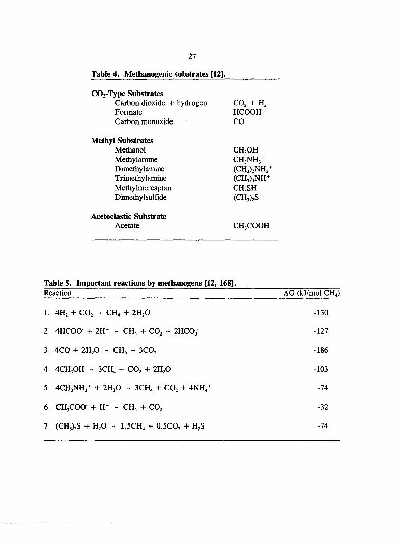
As previously stated, there were 51 reported species of methanogens as of 1991,
grouped into eighteen genera and eight major groups. Table 3 lists the known
methanogens along with their characteristics. The substrates utilized by methanogenic
bacteria consist of approximately 10 simple compounds, and are listed in Table 4 below.
The most common biochemical reactions involved in methane formation are listed
in Table 5. Of the substrates listed, Hj + CO2 and formate are utilized by the most
methanogenic bacterial species. However, it has been estimated that approximately 70%
of the methane formed in nature is via acetate cleavage to methane and carbon dioxide.
This is despite the fact that the free energy associated with acetate cleavage is extremely

26
Table 3. The methanogenic bacteria [12]. Number
Genus Morphology of species Substrates for methanogenesis
GROUP I Methanobacterium Methanobrevibacter
GROUP II Methanothermus
long rods short rods
rods
8 H2 + CO2, formate 3 Hj + CO2, formate
H2 + CO2, reduces S°
GROUP III Methanococcus
GROUP IV Methanomicrobium Methanogenium Methanospirillum
GROUP V Methanoplanus Methanosphaera
GROUP VI Methanosarcina
Methanolobus Methanoculleus Methanococcoides Methanohalophilus
Methanothrix Methanosaeta
irregular cocci
short rods 2 irregular cocci 3 spirilla 1
plate-shaped 2 cocci 1
irregular cocci
irregular cocci 3 irregular cocci 4 irregular cocci 1 irregular cocci 3
rods/filaments 3 rods/filaments 1
H2 + CO2, formate
H2 + CO2, formate H2 + CO2, formate H2 + CO2, formate
H2 + CO2, formate CH3OH + H2
H2 + CO2, formate, CH3OH, methylamines, acetate
CH3OH, methylamines H2 + CO2, formate, alcohols CH3OH, methylamines CH3OH, methylamines, methyl sulfides acetate acetate
GROUP VII Methanopyrus rods in chains Ht + CO-)
GROUP VIII Methanocorpusculum irregular cocci 3 H2 + CO,, formate, alcohols
27
Table 4. Methanogenic substrates [12].
C02-Type Substrates Carbon dioxide + hydrogen CO2 + H2 Formate HCOOH Carbon monoxide CO
Methyl Substrates Methanol CH3OH Methylamine CH3NH3^ Dimethylamine (CH3)2NH2^ Trimethylamine (CH3)3NH^ Methylmercaptan CH3SH Dimethylsulfide (CH3)2S
Acetoclastic Substrate Acetate CH3COOH
Table 5. Important reactions by methanogens [12, 168]. Reaction AG (kJ/mol CH4)
1. 4H2 + CO2 - CH4 + 2H2O -130
2. 4HC00 + 2H^ - CH4 + CO2 + 2HCO3 -127
3. 4C0 + 2H2O - CH4 + 3CO2 -186
4. 4CH3OH - 3CH4 + CO2 + 2H2O -103
5. 4CH3NH3^ + 2H2O - 3CH4 -h CO2 + 4NH4^ -74
6. CH3COO +11^ - CH4 H- CO2 -32
7. (CH3)2S + H2O - I.5CH4 + O.5CO2 + H2S -74

28
low. Additionally, only three genera of methanogens, Methanosarcina, Methanothrix, and
Methanosaeta, have bacterial species capable of utilizing acetate to produce methane and
carbon dioxide [12, 68, 93]. These observations demonstrate the importance of
maintaining a suitable environment for the acetoclastic methanogens. It is also important
to note that for some methanogenic species, the substrate serves as both the energy and
sole carbon source, whereas other methanogens grow only when supplemented with
additional carbon sources. For example, only three genera are capable of splitting acetate
into methane and carbon dioxide (energy production), but several other groups of
methanogens require acetate for biosynthetic purposes [168].
Another important function of the methanogens is maintenance of low hydrogen
partial pressure in the anaerobic environment. The implications of this statement are two
fold: (1) by maintaining a low hydrogen partial pressure (i.e., less than 10"^ atm), the
thermodynamics of the acidogenic and acetogenic bacteria will be favorable (energy
yielding); and (2) by maintaining a low hydrogen ion concentration, the pH of the
anaerobic environment will be maintained within the optimum range (6.5-7.5) for the
methanogens. This second point will be discussed in a later section [23, 47, 93, 168].
Biochemistry of the Methanogens
Because of the importance of the methanogenic bacteria to the overall fiinction of an
anaerobic environment, a general overview of their biochemistry is presented here.
Schematic diagrams of methane production, energy production, and biosynthesis from

29
CO2, methanol, and acetate are presented in Figures 2, 3, and 4, respectively, below. The
pertinent enzymes, coenzymes, and cofactors are indicated where appropriate [12, 168].
Each of these systems is discussed in this section.
Coenzymes and Cofactors. One interesting characteristic of the methanogens is
the presence of several unique coenzymes. The list of unique coenzymes involved in
methanogenesis is long, and a complete description of all of the coenzymes is beyond the
scope of this document. A few of the more important coenzymes are discussed below:
Coenzyme M, or 2-mercaptoethanesulfonic acid (HS-CH2CH2SO3"), is involved in
the terminal step of methane production in all known methanogens. Methane is
produced through the reduction of 2-(methylthio)ethanesulfonic acid to produce
methane and reduced CoM:
CHj-S-CoM + / / j - CH^ + HS-CoM (H)
Despite the importance of CoM for the production of methane, not all methanogens
are able to synthesize CoM, and thus require it as a growth factor. One
methanogen of this type is Methanobrevibacter ruminantium, found in the gut of
rumen animals. CoM is supplied to M. ruminantium by several methanogens which
secrete CoM [12, 168]. Several other enzymes and cofactors are unique to the
methanogens and are described here [12, 112, 168, 170].

30
Coenzyme ^420 is a flavin derivative , similar in structure to the common flavin
coenzyme, flavin mononucleotide (FMN). Coenzyme ^420) however, is a two
electron carrier, rather than a one or two carrier, which is a common characteristic
of many flavin coenzymes. It interacts with the hydrogenases and NADP^
reductases of methanogens, and also plays a role in methanogenesis as an electron
donor in at least one of the steps of carbon dioxide reduction. An interesting
property of coenzyme F420 is its ability to absorb light at 420 nm and fluoresce blue-
green in the oxidized state. This feature presents a useful method of methanogenic
identification [12, 170].
Coenzyme P430 is a nickel-containing tetrapyrrole and plays a crucial part in the final
step of methanogenesis as part of the methyl reductase system. The nickel
requirement of most methanogens is mainly due to coenzyme F430, which is found
in abundance in methanogens [12, 170].
Methanofuran is a low molecular weight coenzyme that interacts in the first step of
methanogenesis from COj. Carbon dioxide is initially reduced to the formyl level
and is bound by the amino side chain of a fiiran ring. The formyl group is
subsequently transferred to a second coenzyme [12].

Methanopterin is a methanogenic coenzyme resembling the vitamin folic acid, and
serves as the C-1 carrier during the reduction of CO2 to CH4. The reduced form,
tetrahydromethanopterin, is the active form of the coenzyme. Methanopterin also
has the property of fluorescence after light absorption at 342 nm [12, 170].
HS-HTP, or 7-mercaptoheptanoylthreonine phosphate, is a cofactor involved in the
final step of methanogenesis catalyzed by the methyl reductase system. The
sulfhydryl active group serves as the electron donor in this final step, resulting in a
disulfide linkage between CoM and HS-HTP (CoM-S-S-HTP) [12].
Enzymes. The specific enzymes involved in all of the steps of methanogenesis
and biosynthesis are complex, and a detaHed description is not presented here. However, a
general discussion of the properties and types of enzymes important in methanogens
follows. The general types of enzymes utilized by methanogens during methane
production include hydrogenases, reductases, dehydrogenases, and transferases.
Obviously, many other enzyme types can be found in methanogens, but those listed are
especially important in the common methanogenic pathways and are discussed below [12,
112, 125, 168, 172].
Hydrogenases bind Hj and split it into protons, which then may be used for ATP
production or serve as reducing equivalents in reduction reactions [12]. The hydrogenase

32
active in methanogenesis from CO2 catalyzes the addition of hydrogen (reduction) to at
least two of intermediates involved.
Generally speaking, a reductase, or oxidoreductase, catalyzes a reaction in which a
molecule is reduced through the addition of electrons, with the simultaneous oxidation of
an electron donating molecule [172]. The methyl reductase system of methanogens is the
most obvious example of this type of enzyme. The methyl group of C0M-S-CH3 is
reduced to methane, with the concomitant generation of a disulfide of CoM-S-S-HTP (HS-
HTP is oxidized) [12, 112, 125, 168, 170].
Transferases catalyze the transfer of a functional group from one molecule to
another [172]. It is generally accepted that there are two main transferases involved in
methanogenesis from methyl substrates, such as methanol (CH3OH). These are generically
termed methyltransferase I and II. Methyltransferase I transfers the methyl group from
methanol to a vitamin B,2 derivative, and methyltransferase II transfers the same methyl
group from B12 to CoM to form methyl CoM [170], The methanopterins do not possess
transferase activity, but they do act as C-1 carriers for most of the reductive steps during
CO2 reduction to methane [12, 168, 170].
Generally, dehydrogenases catalyze the removal of hydrogen from (oxidation) of
molecules [12, 172]. There are several dehydrogenases involved in methanogenesis,
including CO dehydrogenase, which oxidizes carbon monoxide to carbon dioxide, and
formate dehydrogenase, which oxidizes formate to carbon dioxide [168, 170].
33
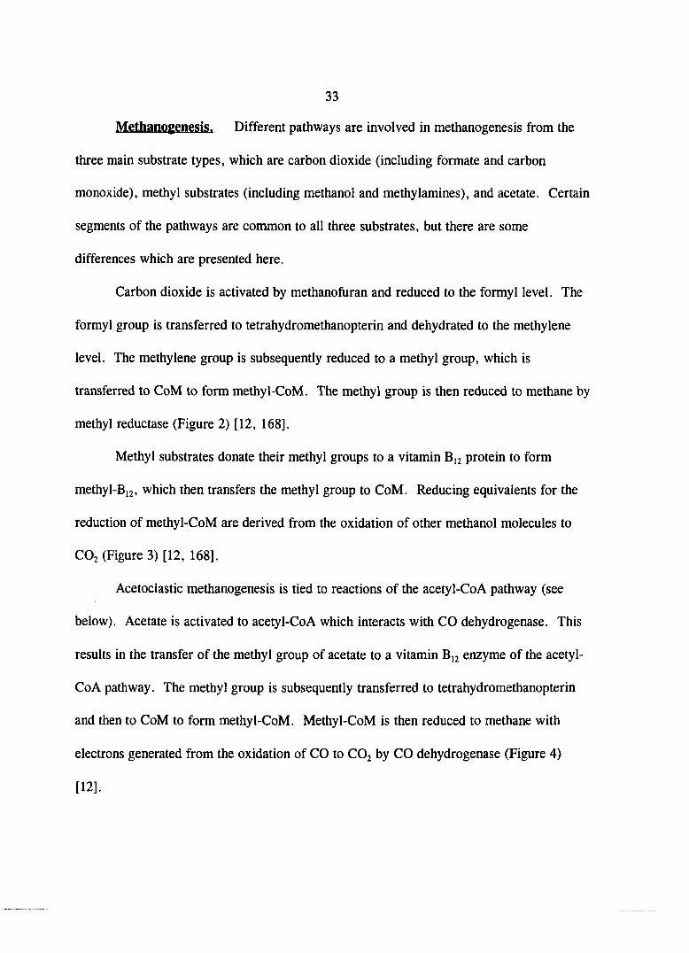
Methanogenesis. Different pathways are involved in methanogenesis from the
three main substrate types, which are carbon dioxide (including formate and carbon
monoxide), methyl substrates (including methanol and methylamines), and acetate. Certain
segments of the pathways are common to all three substrates, but there are some
differences which are presented here.
Carbon dioxide is activated by methanofuran and reduced to the formyl level. The
formyl group is transferred to tetrahydromethanopterin and dehydrated to the methylene
level. The methylene group is subsequently reduced to a methyl group, which is
transferred to CoM to form methyl-CoM. The methyl group is then reduced to methane by
methyl reductase (Figure 2) [12, 168].
Methyl substrates donate their methyl groups to a vitamin B12 protein to form
methyl-B,2, which then transfers the methyl group to CoM. Reducing equivalents for the
reduction of methyl-CoM are derived from the oxidation of other methanol molecules to
CO2 (Figure 3) [12, 168].
Acetoclastic methanogenesis is tied to reactions of the acetyl-CoA pathway (see
below). Acetate is activated to acetyl-CoA which interacts with CO dehydrogenase. This
results in the transfer of the methyl group of acetate to a vitamin B12 enzyme of the acetyl-
CoA pathway. The methyl group is subsequently transferred to tetrahydromethanopterin
and then to CoM to form methyl-CoM. Methyl-CoM is then reduced to methane with
electrons generated from the oxidation of CO to CO2 by CO dehydrogenase (Figure 4)
[12].

34
CO CO
2H CODH
M F - C - H CODH-C 2H MP
2H
CH,- MP CODH-C-CH
CoA CODH
O
CoA-S - C - CH ATP
Cell Material CH^
MF = methanofuran MP = tetrahydromethanopterin CoM = coen^me M CoA = coenzyme A Bi2 = vitamin B|2 CODH = carbon monoxide debiydrogenase
Figure 2. Biochemistry of carbon dioxide utilization by methanogens.

35
CH,OH + B
CoM
MP
CH,-MP 2H
2H ATP
CH
MF
M F - C - H Cell Material
2H
CO2
2H CODH CoA-S - C - CH
CODH-C
CODH-C-CH
MF = methanofuran MP = tetrahydromethanopterin CoM = coen^me M CoA = coenzyme A Bi2 = vitamin ^2 ^ODH^s^caAon^nonoxide^deh^drogeM
Figure 3. Biochemistry of methyl compound utilization by methanogens.

36
CH3COOH
CoA .^I^ATI
( • \ P
CoA-S - C - CH Cell Material
CODH
CODH-C-CH
CODH-C
2H
CO
ATP
CH
MF = methanofuran MP = tetrahydromethanopterin CoM = coenzyme M CoA = coenzyme A Ei[2 = vitamin ^12 CODH = carbon monoxide dehydrogenase
Figure 4. Biochemistry of acetate utilization by methanogens.

37
Although several strains of methanogens utilize CO2, H2, and methyl substrates for
methanogenesis, only a few are able to convert acetate to methane and carbon dioxide.
These are limited to species of the genera Methanothrix, Methanosarcina, and
Methanosaeta (Table 4). Methanothrix and Methanosarcina have especially been
implicated as the major acetate-utilizing bacteria involved in methanogenesis in most
anaerobic systems. The literature cites the three most important species of these genera as
Methanosarcina barkeri, Methanothrix concilii, and Methanothrix soehngenii [70, 76, 88,
90, 110, 168, 169].
Energy Production. Based on experimental evidence, current theory predicts
that many methanogenic bacteria conserve energy by electron transport phosphorylation
[168]. Through this process, a proton motive force is generated, consisting of membrane
potential (inside negative, outside positive) and an pH gradient (inside alkaline, outside
acidic). In addition, a few strains have been isolated that apparently conserve energy
through substrate-level phosphorylation [168].
Proton dependent ATPases have been demonstrated in most methanogens, although
a few strains have been shown to contain sodium dependent ATPases (especially those that
convert methanol to methane). Generally, the terminal step of methanogenesis is the
energy conservation step. The conversion of methyl-CoM is linked to a proton pump that
pumps produced in this step to the outside of the cytoplasmic membrane, thus
establishing a proton gradient and a membrane potential. Membrane-bound proton-

translocating ATPases then dissipate the proton motive force and produce ATP from ADP
and Pi in a fashion that is similar to ATP production in other eubacteria and eukaryotes
[12, 112, 141, 168]. Through thermodynamic considerations, it is generally accepted that
the minimum standard free energy of formation of 1 mole of ATP from ADP and P| is
approximately 31.8 kJ/mol. The conversion of CO2 to CH4 (AG"' = -130.4 kJ/mol),
methanol to CH4 (AG'"= -103 kJ/mol) and of formate to CH4 (AG"'= -119.5 kJ/mol) will
yield a maximum of 3 mole of ATP per mole CH4 produced. The conversion of acetate to
CH4 (AG"' = -32.5 kJ/mol), on the other hand may yield a maximum of only one mole of
ATP per mol methane produced [168].
It is this low production of ATP that is responsible for the low growth rates of
methanogens, especially those that utilize acetate as their methanogenic substrate. For
example, under optimum defined conditions (pH = 7.0, all growth factors and nutrients
provided in excess), doubling times for Methanothrix concilii, Methanothrix soehngenii,
and Methanosarcina barken have been estimated as 3.4 days, 6.7 days, and 3.1 days,
respectively. Further, it is estimated that under normal envirormiental conditions, these
doubling times are considerably longer [70, 90, 110].
Biosynthesis. Methanogenic bacteria synthesize cellular carbon starting from
activated acetate (acetyl-CoA) and COj. Acetate may be taken in directly by the cell when
sufficient acetate concentration exists in the environment, or it may be synthesized from
single- carbon molecules by the following exergonic reactions:
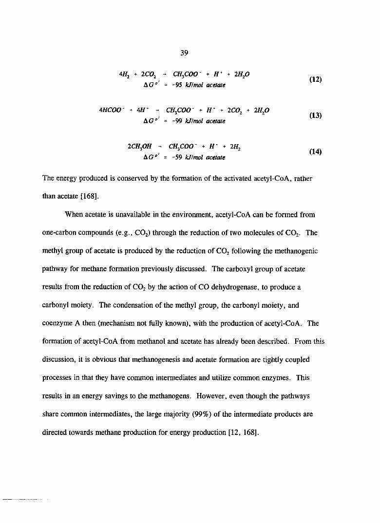
39
4^2 + 2C0^ - CHjCOO + + 2Hp
AG"' = -95 kJImol acetate
4HC00- + AH' - CH^COO + JV + 2C0^ + 2H^O
AG" = -99 kJ/nwl acetate
2CHpH - CH^COO- * ^ 2H^
AG°' = -59 AJ/mo/ acetate
(12)
(13)
(14)
The energy produced is conserved by the formation of the activated acetyl-CoA, rather
than acetate [168].
When acetate is unavailable in the environment, acetyl-CoA can be formed from
one-carbon compounds (e.g., COj) through the reduction of two molecules of COj. The
methyl group of acetate is produced by the reduction of CO2 following the methanogenic
pathway for methane formation previously discussed. The carboxyl group of acetate
results from the reduction of CO2 by the action of CO dehydrogenase, to produce a
carbonyl moiety. The condensation of the methyl group, the carbonyl moiety, and
coenzyme A then (mechanism not fully known), with the production of acetyl-CoA. The
formation of acetyl-CoA from methanol and acetate has already been described. From this
discussion, it is obvious that methanogenesis and acetate formation are tightly coupled
processes in that they have common intermediates and utilize common enzymes. This
results in an energy savings to the methanogens. However, even though the pathways
share common intermediates, the large majority (99%) of the intermediate products are
directed towards methane production for energy production [12, 168].

40
Ammonium ions are used to satisfy the majority of the nitrogen requirement for
methanogens. However, some methanogens have the ability to fix molecular Nj into
cellular nitrogen under limiting ammonia concentrations. Additionally, other methanogens
are not capable of synthesizing all required amino acids. Glutamate accounts for over half
of the soluble amino acid pool in several methanogens, which serves as the main precursor
of the other nitrogen-containing compounds. Formation of other amino acids proceeds
through the action of glutamate-pyruvate transaminase and glutamate-oxaloacetate
transaminase, which connect the various amino acids through a type of tricarboxylic acid
cycle [168].
The sulfiir requirements for methanogens is supplied by reduced forms of sulfur,
such as sulfide or cysteine. The precise metabolic pathways used for sulfur assimilation is
not presently clear. Sulfhydryl groups serve as important active sites in many
methanogenic enzymes and coenzymes, one of which is coenzyme M (which also contains
an oxidized sulfur atom) [168]. Elemental sulfur is also an inhibitor of methanogenesis.
In methanogenic pure cultures growing on hydrogen, the addition of elemental sulfur
inhibited methane formation and resulted in H2S formation [168].
Trace elements required by methanogens include cobalt, iron, molybdenum, nickel,
magnesium, and potassium. The growth of a few methanogens is also stimulated by
tungsten and selenium. The great majority of the trace metal requirement is utilized in the
synthesis of enzymes, coenzymes, and cofactors [168].

41
Interplay among the Anaerobic Bacteria
The previous sections discussed each major group of bacteria in anaerobic
environments as individual, or separate, entities. In actual environments, however, all
groups of bacteria work together to fully stabilize organic material within their
environment. In fact, the various groups depend on the other groups to provide utilizable
substrates, to degrade metabolic end-products, and to maintain appropriate conditions
(e.g., pH) in the environment. Figure 5 depicts the flow of substrates and end-products
among the various groups of bacteria.
The hydrolytic/fermentative bacteria depend on the acetogenic bacteria to degrade
the fatty acids (except acetate) that are produced during fermentation of polymeric
substrates. Additionally, the homoacetogenic and methanogenic bacteria utilize
produced by the fermentative bacteria. Each of these processes improves the
thermodynamic conditions for the hydrolytic/fermentative bacteria, thereby increasing the
energy yield derived from fermentations [47, 81, 93, 168, 170].
The acetogenic bacteria rely on the fermentative bacteria for their carbon and
energy source in the form of fatty acids (3 carbons or longer). As mentioned, the
homoacetogenic bacteria also utilize hydrogen produced in the fermentations. The end-
products of acetogenesis (acetate, CO2, H2) is utilized by the methanogens for energy and
synthesis [47, 81, 93, 168, 170].
Methanogenic bacteria scavenge the H2 produced by both of the other groups of
bacteria, and also utilize COj, formate, acetate, and methanol for growth and energy. The

42
Complex Organic Compounds (Carbohydrates, Proteins, lipids)
1 Hydrolysis
'
Simple Organic Compounds (Sugars, Amio acids, Peptides)
Acidogenesis
Long Chain Fatty Acids (Propionate, Butyrate, etc.)
^Acetogenesis
i—i
Hydrogen
Carbon Dioxide
Methanogenesis
Homoacetogenesis
Methanogenesis
Methane
Carbon Dioxide
Figure 5. Substrate and intermediate product flow among anaerobic bacteria.

Hj-consumption is especially beneficial to the propionate and butyrate-oxidizing acetogens,
since the standard free energy change for propionate and butyrate oxidation is positive
under high hydrogen partial pressure. However, in the presence of methanogens, which
utilize Hj in methanogenesis, the free energy is negative enough to allow energy
production from the oxidation of propionate and butyrate. In some environments,
methanogenic production of CO2 may also provide this starting material for the
homoacetogenic bacteria, which convert two equivalent of COj to acetate. In addition,
by stabilizing the acetate produced by the fermentative and acetogenic bacteria, a proper
pH is maintained in the system so that none of the bacteria in the system become inhibited
by low pH [23, 47, 81, 93, 168, 170].
There are also instances of substrate competition between groups or classes of
bacteria. One example of this is competition between methanogens and homoacetogens for
Hj and COj. Methanogens convert these compounds to methane, whereas homoacetogens
convert them to acetate. In most systems, methanogens are generally able to out-compete
the homoacetogens for CO2 and Hj. Under these conditions, the homoacetogens, which
are capable of heterotrophic metabolism as well as autotrophic, utilize organic compounds
for carbon and energy [168].
A second example of competition for substrates is the well-documented case
between the methanogens and the sulfate-reducing bacteria (SRB) [108, 168]. In the
absence of sulfate, some SRB species actually provide substrates (H2, acetate) to the
methanogens. However, in the presence of sulfate, the SRB generally out-compete the

44
methanogens for H2 and acetate. This is especially significant at high sulfate and low Hj
or acetate concentrations. The SRB have lower values for both and acetate, and,
therefore, have a higher affinity for these substrates than do the methanogens, especially
under limiting conditions of Hj or acetate [108, 168].
Anaerobic Wastewater Treatment
Anaerobic versus Aerobic Treatment
There are generally two biological treatment method for waste stabilization:
aerobic and anaerobic treatment. Aerobic treatment has been widely used for low-strength,
domestic wastewater treatment and also for many industrial wastes. Aerobic bacteria,
because of the high energy yield characteristic of the oxidative phosphorylation pathways
utilized by aerobes, grow very rapidly as compared to the anaerobic bacteria, which gain a
much smaller amount of energy from degradation of a given waste material. Aerobic
bacteria convert some (approximately 1/3 to 1/2) of the waste material to CO2 and water,
with the remaining energy directed towards cell synthesis. The result of this process is the
production of large quantities of biomass which must be further stabilized (usually through
anaerobic digestion) before disposal. Additionally, by definition, aerobic organisms
require molecular oxygen to grow and reproduce. The addition of oxygen to the aerobic
wastewater treatment system, such as an activated sludge system, results in significant
operating costs.

Anaerobic microorganisms, however, require no oxygen, and are, in fact, inhibited
or killed by free oxygen. Therefore, there is no requirement for oxygen addition in
anaerobic waste treatment. Also, since anaerobic microbes reproduce at relatively low
rates (most of the energy of the reactions is lost as methane), the biomass production rate
is low, which further results in lower biomass disposal costs. Another advantage is that
nutrient requirements are lower for anaerobic bacteria, owing to their lower reproduction
rates. An additional benefit to anaerobic treatment is the production of methane, which
contains most (about 90-95%) of the energy of the original waste compound. That is, a
significant portion of the energy of a waste can be captured in the form of methane, which
can then be used to produce electricity or burned to release heat [23, 93].
There are, however, a few disadvantages to anaerobic waste treatment when
compared to aerobic processes. The first is the general requirement for higher operating
temperature for efficient anaerobic waste stabilization. Although there has been and still is
considerable investigation into anaerobic stabilization at lower temperatures, most
anaerobic systems are designed to operate at or near 35°C. However, many, if not most,
anaerobic systems produce more than sufficient methane which can be burned and utilized
for heating the anaerobic reactor. A second disadvantage often cited for anaerobic systems
is the slow growth rates of the methanogenic bacteria, resulting in long start-up periods of
anaerobic systems. This phenomenon has traditionally been confused with low substrate
removal rates. It can not be emphasized enough that these two rates are distinct from each
other. Anaerobic substrate removal rates are similar to aerobic rates. The underlying

46
principal behind the slow methanogenic growth rates is that the methanogens derive very
little energy through methanogenesis, and, therefore, require long time periods to
reproduce [23, 93]. That notwithstanding, the long start-up period for anaerobic systems
is a significant problem and possibly the most significant deterrent to the widespread use of
anaerobic technologies. Many industries are simply not willing to wait for several months
or even years for their waste treatment system to reach design loads.
The problem of long start-up periods, therefore, was selected as one of the items to
be addressed in this research. That is, methods of decreasing the time required to achieve
stable anaerobic degradation of a given wastewater were to be examined in this research.
The methods employed are outlined in a later section.
Environmental/Operational Parameters in Anaerobic Treatment
The parameters affecting anaerobic digestion can be broadly classified as
environmental and operational. Due to the relatively slow growth rates of anaerobic, and
especially methanogenic, bacteria, a longer time is required for these microbes to adjust to
changing conditions within the anaerobic reactor [94]. It is, therefore, desirable to
maintain near optimum environmental and operational conditions in a given anaerobic
waste treatment system. The following paragraphs discuss the important environmental
and operational parameters to efficient anaerobic waste treatment.

47
Environmental Parameters
The main environmental parameters that effect anaerobic digestion are temperature,
pH, alkalinity and volatile acids concentrations, substrate and nutrient availability, and the
presence of toxic or inhibitory compounds. Each of these parameters has an intimate effect
on the overall efficiency of a given anaerobic waste treatment system, and are discussed in
detail.
Temperature. Anaerobic digestion is greatly affected by the temperature at
which the process is carried out. As early as the 1930's, Rudolfs and Heukelekian
reported on noticeable differences in the rate of digestion at different temperatures
(thermophilic and rion-thermophilic). It is generally accepted that the organisms
responsible for digestion at thermophilic temperatures (50 to 70''C) are different from those
responsible for digestion at lower temperatures, such as the mesophilic range (28 to 35°C).
McCarty [94] and several other researchers also found the presence of two distinct
temperature ranges, similar to those given. More recently, psychrophilic (10 to 20''C) has
been investigated for several wastes. It has become apparent that anaerobic digestion may
be carried out within a number of temperature ranges.
Temperature affects the rates at which digestion is carried out, rather than the total
degree of digestion that is achieved. Pidaparti and Dague [25] and Dague [23a] reported
similar total COD and volatile solids destruction at temperatures of both 35°C and 25''C.
However, since the rates of degradation are slower at lower temperatures, the digestion

48
process must be allowed to operate at longer detention times or the biomass population
must increase in order to obtain the same degree of stabilization at lower temperatures.
A general rule of thumb is that microbial metabolism rates (and thus, rates of
digestion) approximately double for each 10°C rise in temperature. This can be shown
mathematically by applying Equation 15 below, which is a conmion temperature correction
equation applied in the wastewater industry.
kr = ^200'""'° (15)
where, ky = rate at the given temperature, T°C, 1/time kjo = rate at 20°C, 1/time T = given temperature, °C 0 = a constant that is specific for the given biological process
For many biological processes, 0 is equal to 1.07. By applying Equation 15 at a
temperature of 30°C, the ratio of kjo/kjo is equal to 1.97, essentially 2. Therefore,
Equation 15 predicts that biological rates will be twice as fast at 30°C as they are at 20°C.
Hydrogen Ion Concentration. The hydrogen ion concentration (pH =
-log[H^]) in an anaerobic reactor has a major effect on the performance of the system.
McCarty [94] suggested a range for pH of 6.6 to 7.6 with an optimum between 7.0 to 7.2.
Other reports have indicated that methanogenesis is possible at pH values as low as 6 to
6.2 and as high as 8.1 to 8.5 [59, 137a, 168]. However, the optimum pH is still quoted as
being 7.0. During the course of the research presented in this document, pH values as low

49
as 6.4 and as high as 7.8 have been observed for short periods of time with little effect on
methanogenesis. Since the methanogens are the most important organisms in an anaerobic
system, it is important that the pH be maintained at a level that is not inhibitory to them,
i.e at pH near neutral. This range of pH has been shown to be the optimum for the
anaerobic process as a whole, not just for the methanogenic organisms.
Alkalinity and Volatile Acids. The alkalinity of a system is a measure of its
capacity to neutralize strong acids without a significant decrease in pH. In most
wastewater applications operating near neutral pH, the main component of alkalinity is the
bicarbonate ion, although carbonate, hydroxyl, phosphate, and borate species also
contribute to alkalinity to varying degrees. Bicarbonate is mainly produced by the
formation of ammonium bicarbonate from CO2 and NH3 during anaerobic degradation of
complex substrates (e.g., protein) by the following reaction;
CO2 + NHj + Hp - NHfiCO^ (16)
The ammonium bicarbonate dissociates to NH4^ and HCOj'. The bicarbonate ion provides
a buffer to decreases in pH through the carbonic acid/bicarbonate system, as shown in
Equation 17.
^ Hco; + (17)

Examination of Equation 17 shows that the carbonic acid-bicarbonate system is directly
influenced by the pH of the reactor and vice versa. Therefore, as acid (H"^) is added to the
system, bicarbonate is used to produce carbonic acid (which is also in equilibrium with
carbon dioxide and water), but the pH of the system will not decrease significantly until
the majority of the bicarbonate is gone. Additionally, ammonium is in equilibrium with
ammonia and protons. However, the pKg of the NH4^/NH3 system is approximately 8.95
at 35°C, and, therefore, provides little buffer capacity in most treatment systems [53],
Many wastewaters do not contain sufficient alkalinity to maintain proper pH levels over the
course of treatment. In these applications, it is usually necessary to add alkalinity to
ensure maintenance of appropriate pH. Common alkaline compounds used for this are
ammonia, lime, sodium bicarbonate, and sodium hydroxide [23, 94, 96].
Volatile organic acids are produced through the degradation of more complex
molecules by the acidogenic and acetogenic bacteria. If the volatile acid (acetic, propionic,
butyric) concentration increase to high levels, the pH of the system may be depressed due
to the equilibrium established between the acids and their respective salts. Equation 18
represents the produced by acetic acid ionization.
CH^COOH ^ CHjCOO- + H' (18)
Since the pK^ of most of the volatile acids is less than 4, most of the acid will be present in
the ionized form, thus producing with a subsequent decrease in pH unless sufficient
alkalinity exists to neutralize the acid. A high volatile acids concentration in conjunction

with low pH (< 6.5) is a prevalent problem with improperly operated anaerobic systems,
and is conunonly known as a "stuck" digester. In order to relieve this condition, the pH
must be raised to non-inhibitory levels with an alkaline material, often lime. The
methanogens may then function properly to remove the acids and produce methane. It has
been noted that it is the low pH, rather than high volatile acids concentration, that inhibits
proper anaerobic digestion; therefore, the pH is the single most important environmental
parameter for efficient anaerobic treatment [23, 94, 96].
Nutrient and Trace Element Availahilitv. Although anaerobic bacteria grow at
a relatively slow rate, they do require nutrients (nitrogen, phosphorous, sulfur, potassium,
sodium, and others) and trace elements (iron, nickel, copper, zinc, and other metals) in
small quantities for efficient growth and methanogenesis [106, 142, 148, 149]. Nitrogen
and sulfiir are incorporated into cellular material, such as proteins, and phosphorous plays
an important role in the high energy phosphorous bonds in which chemical energy is stored
as ATP and other energy-storage molecules. Sodium and potassium are mainly used to
maintain the ionic strength of the cytoplasm at appropriate
levels, as well as playing a role in ATP production in some ATPases [18, 19, 59, 65,
168].
Heavy metals are incorporated into the various enzymes, coenzymes, and cofactors
of the anaerobic bacteria. Often, the heavy metals are important constituents of the active
sites on enzymes and coenzymes [18, 19, 65, 106, 168, 172]. The nutrients and trace

52
elements listed here are necessary in low concentrations, and in a properly operated system
are not the limiting compounds. However, care must be taken so that the concentrations of
these compounds are not high enough to cause inhibition, as presented below [95].
Toxic or Inhibitory Compounds. Many organic and inorganic materials may be
toxic to anaerobic organisms. Often, at low concentrations, these same materials may be
stimulatory to the microorganisms, but as the concentration of the material increases, it
becomes inhibitory and finally toxic. The alkali and alkaline-earth metals are examples
of compounds that exhibit this phenomenon [95, 121], McCarty [95] reported on the
effects of several alkali and alkaline-earth metals on anaerobic digestion. His summary is
presented in Table 6.
Ammonia, although necessary for cellular biosynthesis, can be toxic at higher
concentrations. As earlier stated, ammonia is in equilibrium with ammonium, and the
pKa of the system is 8.95 at 35''C (Equation 19). Therefore, at a pH of 7.0, it can be
Table 6. Effects of alkali and alkaiine-earth metals on anaerobic digestion [95]. Concentration (mg/L)
Moderately Strongly Cation Stimulatory Inhibitory Inhibitory
Sodium 100-200 3,500-5,500 8,000
Potassium 200-400 2,500-4,500 12,000
Calcium 100-200 2,500-4,500 8,000
Magnesium 75-150 1,000-1,500 3,000

aw; NH^ + H' (19)
calculated that the ratio of NH3 to NH4^ is 0.011 (10 ®^^/10"' °). Stated differently, 98.9%
of the ammonia pool will be in ionic form, which is the less toxic form of the two species.
McCarty stated that a total anmionia concentrations of 50 to 200 mg/L was beneficial to
anaerobic waste treatment. Total ammonia concentrations of 200 to 1,000 mg/L have no
adverse effects, whereas concentrations of 1,500 to 3,000 are inhibitory, especially at high
pH values. Greater than 3,0(X) mg/L of total ammonia was stated to be toxic to the
anaerobic system [95].
Parkin et al. [109a] reported on the effects of industrial toxicants to methane
fermentation. The study reported on the toxicity of nickel, ammonium, sulfide, and
formaldehyde. In all cases, the inhibition to the methanogenic bacteria appeared to be
reversible, and acclimation of the biomass to the toxicant occurred, indicating the
inhibition to toxicants can be overcome with time. The authors state that a long solids
retention time (SRT) is the best safeguard against failures of a treatment system that must
handle toxicants.
Heavy metals have also been reported to inhibit methanogenesis. Copper, zinc, and
nickel have all been associated with digestion problems due to relatively low concentrations
of the soluble metals. Sulfate may also inhibit methanogenesis due to the competing
reactions of the sulfate-reducing bacteria [120, 154]. Under normal sulfate concentrations.

though, sulfate is reduced to sulfide with little effect on methanogenesis. Sulfide has also
been observed to be inhibitory at low concentrations. However, when heavy metals and
sulfides exist together, they combine to form extremely insoluble precipitates of metal
sulfides. Additionally, slowly- or non-biodegradable organic compounds and inorganic
compounds may inhibit anaerobic digestion if present in high enough concentrations. The
best remedies for treatment of such wastewaters is removal of the compound prior to
anaerobic treatment, or dilution of the wastewater so that the concentration of the
compound is below inhibitory levels [65, 95, 120].
Operational Parameters
Operational parameters are those that are under direct control of the operator.
These parameters include solids retention time, organic loading rate, and hydraulic
retention time. Control of these parameters defines the loading criteria of the anaerobic
system.
Solids Retention Time. The solids retention time (SRT) of an anaerobic system
is a reflection of the average time that a solid particle is retained in the system. If the SRT
is less than the microbial regeneration time of the slowest growing organism, the proper
consortium of anaerobic bacteria may not be maintained in the system [26]. Since the
slowest growing anaerobes are the methanogens, SRT control is especially beneficial to
these organisms. The SRT of a system is defined as the mass of solids in a system divided

by the mass of solids lost from the system per time. If the biomass inventory (MLSS) of a
system is in equilibrium, the SRT may also be defined as the mass of solids in the system
divided by the mass of solids produced per time, since the mass produced is equal to the
mass lost (Equation 20).
SRT = of solids within the system mass of solids lost per time
The required SRT is dependent on the temperature of the system since, as
temperature increases, microbial regeneration times decrease. Therefore, at high
temperatures, the required SRT is less than that required at lower temperatures.
Dague et al. [26] reported that the required SRT for stable anaerobic treatment at 35"C is
approximately 10 days. Because of increased metabolic rates at higher temperatures, the
minimum SRT at a temperature of 55°C is only 2 to 3 days.
The SRT has an effect on the degree of stabilization of the organic content of a
waste. As the SRT is increased beyond its minimum, removal rates of organic material
increase and gradually plateau as the SRT becomes very long [26]. As the SRT becomes
less than 10 days (at 35°C), some of the methanogens will be lost from the system at a rate
faster than the rate at which they reproduce. As this situation continues, the concentration
of acetic acid begins to increase. As the SRT continues to decrease, longer-chained
volatile acids (propionic and butyric) begin to increase in concentration because the
hydrogen partial pressure will also rise due to decreased hydrogen removal by the

56
methanogens. Failure of the anaerobic system is close at this point, and the SRT must be
increased to avoid complete failure [23, 26, 96].
Hydraulic Retention Time. The hydraulic retention time (HRT) is the average
amount of time that a molecule of water is retained within the reactor. In the case of a
completely-mixed reactor, the HRT is equal to the SRT. The HRT is mainly important in
that it affects the organic loading rate (described below). From a cost perspective, it is
advantages to operate an anaerobic treatment system for a give wastewater at the minimum
possible HRT. This results in a smaller reactor volume and less capital cost. Typical
HRTs for municipal digesters range from 15 to 40 days. High-rate anaerobic processes are
often operated at HRTs of 48, 24, 12, or even 6 hrs. HRTs less than 3 hours have been
reported for anaerobic filters treating domestic strength wastewater [31a].
The HRT also affects the SRT of the system to an extent. If the biomass inventory
of a system is the same for two different HRTs, and the concentration of biomass in the
effluent from the system is also constant, then the low HRT system will operate at an SRT
of one-half of the long-HRT system. This is because more liquid passes through the short-
HRT reactor over a given time period, and thus, more solids will be carried out of the
system, everything else being equal. For a suspended-growth system in which the solids
inventory and effluent solids can be measured directly, the SRT can be calculated in terms
of the solids inventory, effluent solids, and HRT (Equation 21):
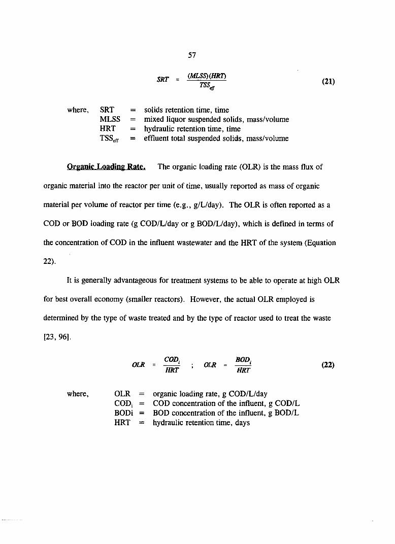
57
SRT - (MLSS>mT> ^21) TSS^
where, SRT = solids retention time, time MLSS = mixed liquor suspended solids, mass/volume HRT = hydraulic retention time, time TSSeff = effluent total suspended solids, mass/volume
Organic Loading Rate. The organic loading rate (OLR) is the mass flux of
organic material into the reactor per unit of time, usually reported as mass of organic
material per volume of reactor per time (e.g., g/L/day). The OLR is often reported as a
COD or BOD loading rate (g COD/L/day or g BOD/L/day), which is defined in terms of
the concentration of COD in the influent wastewater and the HRT of the system (Equation
22).
It is generally advantageous for treatment systems to be able to operate at high OLR
for best overall economy (smaller reactors). However, the actual OLR employed is
determined by the type of waste treated and by the type of reactor used to treat the waste
[23, 96],
COD, BOD, OLR = ; OLR = (22)
HRT HRT
where, OLR = organic loading rate, g COD/L/day CODj = COD concentration of the influent, g COD/L BODi = BOD concentration of the influent, g BOD/L HRT = hydraulic retention time, days

58
Early Research
Approximately 30 years after Pasteur discovered anaerobic life in 1861, the first
anaerobic processes were employed for waste stabilization. Anaerobic bacteria were first
applied to waste stabilization in the 1890s in a combined process of clarification
(sedimentation) and sludge digestion (the septic tank). Interestingly, the septic tank is still
used today in rural areas not serviced by municipal sanitary sewers. Prior to the septic
tank, cesspools were utilized for wastewater disposal, which were little more than
sedimentation basins in which anaerobic decomposition occurred, although the mechanism
of anaerobic treatment was not understood at the time [23].
In 1906, Travis proposed the use two-story tanks to separate sedimentation from
solids digestion, and, in 1907, the German Karl Imhoff developed the two-story "Imhoff"
tank. This process employed an upper level in which the influent wastewater was clarified
by sedimentation, and a lower level in which anaerobic digestion occurred. The Imhoff
tank became popular during the first three decades of the 1900s and were installed in over
240 cities throughout Europe and the United States. The most common problems with the
Imhoff tank were odors and scum formation [23].
In 1918, John Alvord constructed the first system of separate sludge digestion in
the city of Madison, Wisconsin. The system consisted of a clarifier and a separate tank for
digestion of the solids. The solids were removed hydraulically from the sedimentation
tanks, which alleviated the problem of rising sludge into the settling zone, which was a
characteristic problem of the Imhoff tank. Separate sludge digestion was first incorporated

into a wastewater treatment plant in 1923 in Brownsville, Texas. The next major
modification to anaerobic digestion processes was the heating of the digestion tanks, which
was first practiced in Antigo, Wisconsin, in 1926. Within five years of that date, over 100
plants serving 3.5 million people in the U.S. were practicing heated digestion [23].
Temperature effects on solids digestion were widely researched during the 1930s at
temperatures ranging from less than 10°C up to 60''C. Numerous optimum temperatures
were cited, but it was noted by several researchers that digestion rates increased at
increasing temperatures. Additionally, it was observed that the total stabilization and gas
production at different temperatures were similar, but that stabilization required longer
time periods at lower temperatures. In the latter 1930s, multi-stage digestion was
employed, with the first stage operating at thermophilic temperatures and the second stage
at mesophilic temperaftares [23].
The first reports of the importance of the solids retention time, rather than the
liquid detention time, came about in the 1940s. Schlenz reported on a system that operated
at a 60-day solids detention time and a 30-day liquid detention time, which was achieved
by transferring a larger volume of the supernatant (rather than the settled sludge) to the
second stage digestion unit. A further report of this phenomenon was the application of
two stage digestion to a wastewater from a yeast manufacturer. The system operated at
approximately a four-day liquid detention time and decreased the five day biochemical
oxygen demand (BOD5) from 5,000 mg/L to 1,100 mg/L. This was one of the first
applications of anaerobic treatment to a liquid waste, rather than a sludge [23]. In 1950,

60
Rawn and Candell reported on a four-stage digestion system which employed the recycling
of settled sludge from the fourth to the first stage. Although not stated by the authors,
this, in effect, increased the solids retention time (SRT) of the system and the amount of
biomass in the digesters [23].
High-Rate Anaerobic Treatment
The Anaerobic Contact Process
The first "high-rate" process for anaerobic treatment appeared in the literamre in
1953. Fullen reported on a process that was being studied in Austin, Minnesota, treating a
packing house wastewater in which the influent wastewater was mixed with an activated
anaerobic sludge at a temperature of 92 to 94°F. The mixed liquor was then taken to a
clarification basin and separated from the supernatant by degasification and sedimentation.
After sedimentation, the anaerobic biomass was returned to the digester to complete the
cycle. The process, which was later called the anaerobic contact process (Figure 6),
reduced the BODj of the wastewater by 95% in a liquid detention time of 24 hrs or less.
The anaerobic contact process, analogous to the aerobic activated sludge process, could
handle more than 0.20 lb BODs/ftVday, which was four times greater than typical activated
sludge BOD loading rates. This was attributed to the greater mixed liquor concentrations
that could be maintained in the anaerobic contact process: up to 15,000 mg/L as compared
to 2,000 to 3,000 in aerobic activated sludge systems. In 1957, this system was applied to
sewage wastewater with similar (although poorer) results at temperamres of 4 to 25''C [22,

61
Biogas
Mixer
Degasification
Sedimentation
•v. -v. •/. •.!
*,• /,• /.• /.• .*,• .*,• ;
^*^VO^^V.;V.;V.^V<,VO^V^^
Efnuent
.• •
• .*.• .*,• .*,• /.• .*,• .*.•
•'»' 'V •;
Contact tanl(
'•\'y''y''y»'y'*y''y''y/ysy/, ,*. •/. •.*• *. • •.
•' /.*• •*.'• •'.*• %*• •'/• */• **.••
Sludge return Influent
Figure 6. The anaerobic contact process.
23]. Other full-scale installations of the anaerobic contact process have been reported [9,
28],
The Anaerobic Filter
The first reports on the anaerobic filter (Figure 7) were presented by McCarty in
1966 and Young and McCarty in the 1969 [23, 167a]. Their anaerobic filter was packed

62
Biogas
Fully-paclied Alter
i,^^£fnuent
Recycled Effluent
Influent
Figure 7. The anaerobic filter.
with quartzite stone media for microbial attachment, similar to the aerobic trickling filters
popular for domestic wastewater treatment plants. The typical anaerobic filter operates in
an upflow mode, with the influent waste stream entering at the bottom of the filter and
exiting at the top. However, some anaerobic filters are operated in a downflow mode,
with the influent waste stream entering at the top and the effluent exiting at the bottom.
Recycle of the effluent to the influent line may or may not be practiced. The anaerobic

63
filter was the first of the so-called second-generation anaerobic treatment processes, which
allowed the attainment of very long SRTs without the requirement of returning sludge to
the reactor. Rather, the biomass attaches to the media and is caught in the interstitial
spaces between the attachment media, and is thus retained in the reactor rather than exiting
with the liquid effluent.
In Young and McCarty's paper, the authors point out that the anaerobic filter has
many advantages over conventional biological treatment processes, including: (1) the
anaerobic filter is suited for treatment of soluble wastes, (2) no effluent or solids recycle is
required, (3) dilute wastes can be treated efficiently because of the accumulation of high
concentrations of biological solids (long solids retention time), and (4) very low volumes
of sludge are produced, which reduces sludge disposal costs.
The first anaerobic filters of Young and McCarty were operated at 25°C with the
flow introduced at the bottom of the filter and exiting at the top without recycle. The
filters consisted of plexiglass columns filled with smooth quartzite stone (1 to 1.5 inches in
diameter); the completed filter had a porosity of 0.42. Two separate synthetic substrates
were studied: a protein-carbohydrate mixture and a volatile acid mixture (acetic acid and
propionic acid). Compared to modern anaerobic filters, the filters were operated at
relatively low organic loading rates (0.4 to 3.4 g COD/L/day) with COD removals near or
above 90 percent except at the higher loadings. The authors obtained the higher organic
loadings by decreasing the hydraulic retention time (HRT) to as low as 4.5 hours (based on
the void volume of the filter). Significant washout of biomass occurred at these low

64
HRTs, resulting in poor COD removal efficiencies [167a]. Hentz and Harremoes [55]
presented a comprehensive literature review on waste treatment using anaerobic filters.
The Hybrid Anaerobic Filter
The anaerobic filter became popular during the 1970s because of its loading and
hydraulic capacity and its ease of operation. However, plugging of the media over time
resulted in channeling of the influent through the filter and decreased organic removal
efficiencies. A modification to the anaerobic filter was made by removing the lower
portion (one-third to two-thirds) of the attachment media. The new reactor, termed the
hybrid anaerobic filter, or the upfiow blanket filter (UBF), reduced the chances of
plugging by having a suspended growth system in the bottom of the filter (Figure 8).
However, the media at the top of the filter was still able to maintain high biomass
concentrations within the filter. Additionally, capital costs are reduced because of the
smaller amount of filter media required.
Guiot and van den Berg [13] studied a UBF which consisted of an open volume in
the bottom two-thirds of the reactor with the top third containing plastic rings as the
support media. The authors used a soluble sugar waste as the substrate. The reactors
were operated at 2TC. The COD removal efficiencies were above 95% for loads up to 25
g COD/L/day. Similar removal efficiencies were obtained when the HRT was reduced to
as low as 3 hours. Droste et al. [10] used a similar UBF to treat domestic strength

65
Suspended Biomass
Partially-packed filter
-Effluent
Recycled Effluent
Influent
Figure 8. The hybrid anaerobic Alter.
wastewater (300-1,000 mg COD/L) at 27°C. Results indicate that 95% soluble COD
removal efficiency at HRT's down to 3 hours were possible.
The Expanded-Bed Anaerobic Reactor
The expanded-bed reactor (Figure 9) was developed in order to overcome the
problem of clogging that sometimes occurs in the upflow anaerobic filter. The expanded-
bed reactor is operated similarly to the anaerobic filter, except that the fixed attachment
media of the filter is replaced by a granular matrix which does not occupy the entire
reactor volume. The matrix may occupy one-third to one-half of the reactor volume when

66
Biogas
Effluent
Attachment Media
(suspended) Recycled Effluent
Influent
Figure 9. The anaerobic expanded-bed (fluidized-bed) reactor.
allowed to settle to the bottom of the reactor. However, during operation of the expanded-
bed reactor, the upflow velocity of the influent wastewater causes the matrix to expand and
become fluidized. Bacteria attach to the matrix, which may consist of sand, granular
activated carbon, glass beads, or a number of other materials. It is normally necessary to
recycle effluent to the reactor in order to obtain the upward liquid velocities necessary to
fluidize the bed. The granular matrix provides a large surface area for biomass attachment

and also precludes clogging of the reactor due to the high porosity inherent in the fluidized
bed. A basic disadvantage of the process is the high effluent recirculation required to
expand the media bed. Another problem which has been encountered is one of changing
specific gravity of the matrix. For example, initially, the sand used for the matrix may
have a specific gravity of 2.5. However, after bacterial attachment and growth, the overall
specific gravity of the sand/bacterial matrix may be considerably less. If the upflow
velocity is kept constant, particles may be washed out of the reactor over time due to their
decreased specific gravity (decreased settling velocity).
Wang et al. [159] studied the treatment of an acetic acid wastewater using the EBR
with granular activated carbon as the media. The reactor was operated at 35°C, and a bed
expansion of approximately 25% was maintained by recirculating effluent at about 1,000
times the influent feed flow rate. The HRT was maintained constant (value not given), and
the acetate concentration in the feed ranged from 8(X) mg/L to 6,400 mg/L. The results
showed that removal of acetic acid and COD exceeded 98 and 97%, respectively, for all
concentrations studied (steady-state). The authors also note that the EBR responded
positively to sudden increases in the organic load. A doubling of the organic load caused
an almost immediate doubling in the gas production rate.
Fox et al. [38] compared the performance of EBR's with respect to media types.
The media types used were low-density anthracite (0.7 mm average diameter), granular
activated carbon (0.7 mm average diameter), and two sizes of sand (0.35 and 0.7 mm
average diameters). Temperature was 35°C, bed expansion was 50%, and acetate was used

68
as the sole organic source. The HRT and organic loading rate were maintained at 12 hours
and 10.6 g COD/L/day, respectively. Results from this study show that removal
efficiencies for all media were consistently greater than 90%. The granular activated
carbon (GAC) accumulated biomass at a faster rate during start-up than the other media
studied, and, therefore, required less time to reach maximum efficiency based on COD
removal.
The Upflow Anaerobic Sludge Blanket Reactor
One of the most widely-used of the so-called second generation anaerobic reactors
is the upflow anaerobic sludge blanket reactor (UASB), which was introduced in 1980 by
Lettinga et al. [85]. The UASB had been smdied in Lettinga's laboratory in The
Netherlands since 1971. The UASB is a continuous-flow, suspended growth system that is
similar to the anaerobic filter, except that the UASB contains no attachment media (Figure
10). Wastewater enters the UASB at the bottom and exits at the top. The UASB relies on
the formation of a "sludge blanket" which forms when the upflow velocity of the
wastewater is equal to or less than the settling velocity of the biomass. The blanket is, in
effect, suspended in the bottom portion of the reactor. Wastewater flows upward through
the blanket, where the organic constituents of the wastewater are metabolized.
The authors studied many different substrate types and loading combinations, and
found that the UASB could handle organic loading rates in excess of 25 g COD/L/day at
HRTs as low as 3 hours. An important operational characteristic of the UASB is the

69
Biogas
Stratified Sludge Bed (suspended)
.^^JEffluent
Recycled Effluent
i Influent
Figure 10. The upflow anaerobic sludge blanket reactor.
formation of a sludge of superior quality with respect to settling and specific gravity. The
formation of this sludge, known as granular sludge, was thought to be the result of a
combination of factors: (1) the sludge was exposed to varying forces of gravity
compression; (2) the creation and maintenance of favorable conditions within the reactor,
especially the presence of calcium ions and other nutrients, gentle mixing from gas
releases, and the absence of a high concentration of poorly flocculating suspended matter
70
in the wastewater; and (3) the finely dispersed fraction of the sludge will naturally be
washed out with the effluent, leaving the high quality sludge behind.
In a later paper, Lettinga et al. [84] studied the effect of temperature on the UASB
reactor performance. The UASB was shown to be efficient in the treatment of several
wastes (volatile fatty acids, alcohol, potato processing) at temperatures ranging from 19 to
35°C. The COD loads ranged from 3 to 62 g/L/day, and COD removals (filtered) were
consistently greater than 90%. Numerous other studies by these and other authors report
on the UASB as applied to various wastes under varied conditions [13, 37, 69, 78, 83,
132, 133, 139, 157, 160, 166].
It is generally accepted that the performance of the UASB depends largely on the
formation of a granular sludge. The mechanisms responsible for granular sludge formation
are not well understood, however. The phenomenon of granulation is discussed in detail in
a later section.
The Anaerobic Sequencing Batch Reactor
Background and Fundamentals. A relatively new high-rate anaerobic process,
termed the anaerobic sequencing batch reactor (ASBR, Figure 11), was developed in the
late 1980s in the environmental engineering laboratories at Iowa State University under the
direction of Dr. Richard Dague. Initial research on the ASBR dates back to the 1960s at
which time Dague conducted research on "anaerobic activated sludge" as part of his
doctoral research [23a]. At that time, it was recognized that the process could achieve

71
-Biogas Mixer
Floating Gas Cover
. • •. • •, •'. •". • •/• •/• *,'• -.*• -.•• •/• •/• •.•• • .* • »• • • • .* • •* • .* • .• • .* • •• • .* • .* • •• • I • *.*».* • .• • .• .%• .*.• *.* .**• .*.• ••.• .*.• .*••
••••.• •*.*• •\'V/'V^V/'V.'.V.'V.'V/Vh-
"•'y/yfyfy/yfyfyfy/y^^^^ u*. •/. •/. •/. •/• •/• •. • •.•. •.•. •/. ',•• •/• ••*
Effluent
•>/y/y/y/y/y^ •:• ' " " '' *. %*. •, •• %•• •/• •/» •.*• •/. ».*• •/. *
Suspended Biomass
*. * «•* •«•••• •»•* •»•' \* \* •••* •••* •.*•* •.« •.' r. V •. V *..* *..• •• V •. V •. / *• V *•.* •• V *•. V^v^v^v^v^^^ •v^v^v.-v.
>/y/y/y/:>/y^/0/0/y^ •/. •.*. •.*• •.'• *.'• •/• •.*• •/• •.*• •.'
-. •.*•»•••*•.* • .* • .* • .* • •* • t • .* • .* • .• •
: *.• .*.• .*.• .*,• .*.• .*.• .•.« .*.•
^•y/y/y/y:y/y/y/y^ Influent
Figure 11. The anaerobic sequencing batch reactor.
long SRTs while maintaining a low HRT due to internal clarification of the biomass prior
to decanting. Some twenty years later, the concept of the anaerobic batch reactor was
revisited, resulting in several preliminary studies on the ASBR [24, 25, 48, 73, 116].
Since the ASBR is the topic of this document, a detailed description of the ASBR process
and applications of the process to waste treatment follows.
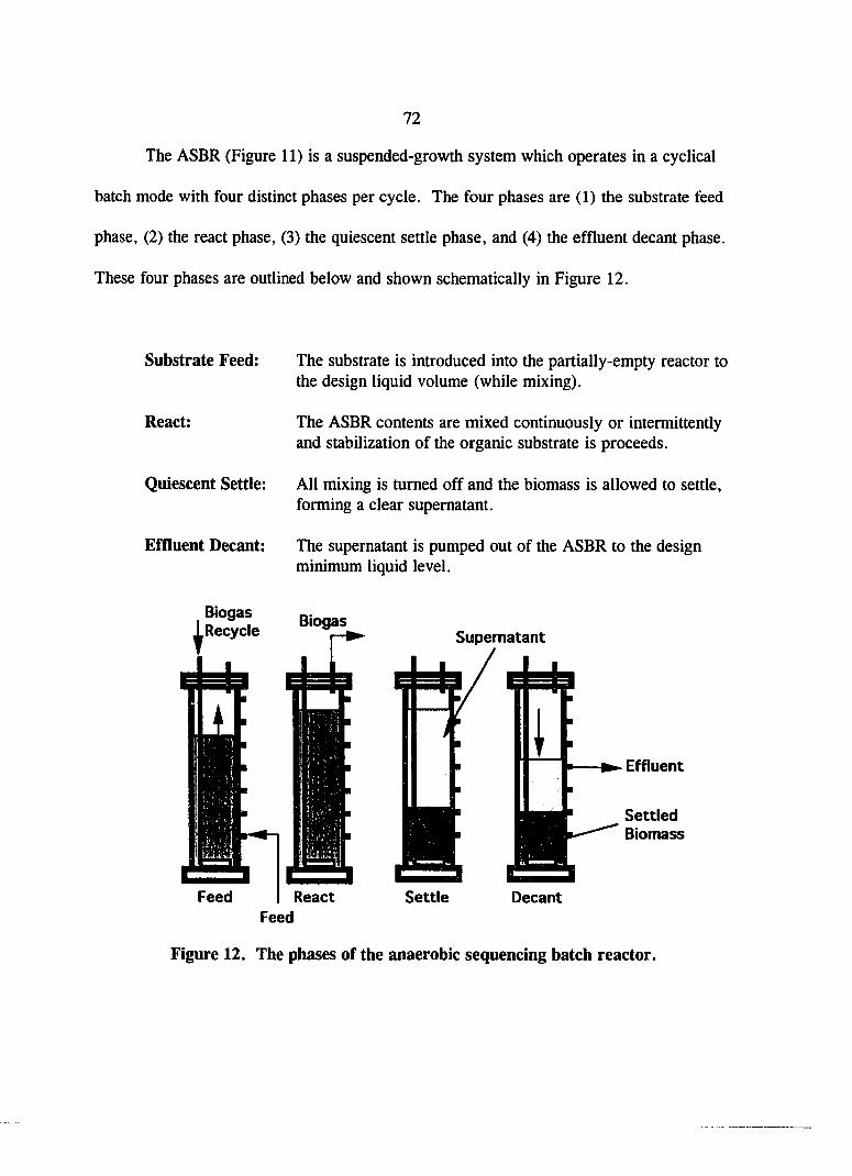
72
The ASBR (Figure 11) is a suspended-growth system which operates in a cyclical
batch mode with four distinct phases per cycle. The four phases are (1) the substrate feed
phase, (2) the react phase, (3) the quiescent settle phase, and (4) the effluent decant phase.
These four phases are outlined below and shown schematically in Figure 12.
Substrate Feed: The substrate is introduced into the partially-empty reactor to the design liquid volume (while mixing).
React: The ASBR contents are mixed continuously or intermittently and stabilization of the organic substrate is proceeds.
Quiescent Settle: All mixing is turned off and the biomass is allowed to settle, forming a clear supernatant.
Effluent Decant: The supernatant is pumped out of the ASBR to the design minimum liquid level.
Biogas Recycle Biogas
Supernatant
Settle Decant
Effluent
Settled Biomass
Feed
Figure 12. The phases of the anaerobic sequencing batch reactor.

73
The batch mode of operation inherently selects for optimum reaction kinetics during
the four phases of operation. During the feed and the initial part of the react phases, the
substrate concentration is at its maximum level. During the settle and decant phases, the
substrate concentration is at its minimum level. The Monod function [81] can be used to
describe the substrate removal rate as a function of the substrate concentration (Equation
23 and Figure 13). Examination of the Monod function reveals that at low substrate
concentrations (settle and decant phases of the ASBR cycle) the substrate removal rate is
low. Therefore, the biogas production rate is also low, creating optimal conditions for
biomass sedimentation. Conversely, at high substrate concentrations, the removal rate
(and biogas production rate) is high, providing fast metabolism of the substrate and internal
gas mixing for better biomass-substrate contact. Within the context of the ASBR, the
substrate concentration decreases over a cycle period, resulting in a decreasing
substrate removal rate and biogas production rate over a cycle period.
ds
•a ' tri
where, s = substrate concentration in the reactor, mass/volume km = maximum specific substrate removal rate (mass of substrate
removed per unit biomass per time), time ' Kg = half velocity constant equal to the substrate concentration at which
ds/dt is equal to Vi the maximum substrate removal rate (k^), mass/volume
M = amount of biomass in the reactor, mass/volume t = time

74
theoretical maximum rate, km or (im
Substrate removal rate, k (1/time)
or J^2 jQaxilpujQ r^Je
Biomass growth rate, |i (l/time)
Substrate Concentration, s (mass/volume)
Figure 13. Graphical representation of the Monod function.
Figure 14 represents a tlieoretical substrate concentration curve over four cycles of
ASBR operation. Note that at the end of each cycle, the substrate concentration is a
minimum, resulting in a well-settling biomass just prior to the decant phase of each cycle.
Another advantage to the ASBR is that substrate conversion and biomass
sedimentation occur in one reactor, eliminating the need for a separate clarifier (as in the
anaerobic contact process), and saving capital costs. As previously stated, mixing may be
performed continuously or intermittently. Dague et al. [26], and Sung and Dague [145]
reported on the use of intermittent mixing rather than continuous mixing. Both of them

75
I Cycle 1 Cycle 1 Cycle 1 Cycle
Maximum F/M Ratio
Average F/M Ratio
Substrate Concentration
Biogas Production
Minimum F/M Ratio
Time
Figure 14. Theoretical substrate concentration and F/M ratio over time in the ASBR.
observed equal or greater COD removal efficiencies with intermittent mixing as compared
to continuous mixing. The researchers also observed better clarification of the supernatant
with intermittent mixing, most likely due to less shearing of the biomass floes.
Research on the ASBR. The first smdy devoted to the ASBR process was
conducted by Habben and Dague in the latter 1980s and the 1990s [24, 25, 48]. The
ASBRs of this study had liquid volumes of 13 liters and were fed a synthetic substrate
consisting of non-fat dry milk plus appropriate nutrients and trace elements. HRTs of

76
0.54, 1.08, and 2.17 days and COD loadings ranging from 0.5 to 5 g/L/day were
investigated at 35°C. This initial system was capable of 80% COD removal (at the two
longer HRTs) when the COD load was 3 g/L/day or less. Higher COD loads resulted in
decreased efficiency and failure of the system at 5 g COD/L/day.
Pidaparti [116] and Schmit [136], in 1991 and 1992, respectively, reported on the
ASBR treatment of swine waste at 35, 25, and 20''C. It was found that at 35°C (HRT = 6
days), volatile solids (VS) loading rates of 1.09 to 5.38 g/L/day were investigated, with the
volatile solids destruction ranging from 87 to 74%, respectively. At 25°C (HRT = 6
days), VS loading rates of 1.04 to 6.82 g/L/day were treated to VS destruction efficiencies
of 92 to 77%, respectively. At 20°C (HRT = 6, 9, and 12 days) the VS destruction
decreased to an extent. At VS loadings of 0.9 to 5.4 g/L/day, VS destruction ranged from
40 to 70%, but was generally about 50% at VS loading rates greater than 2 g/L/day.
Kaiser [73] studied the ASBR treatment of non-fat dry milk at thermophilic
temperatures (55°C). The writer demonstrated the capability of the ASBR to achieve stable
treatment at COD loadings as high as 9 g/L/day at HRTs of 1, 2, and 5 days. This
compared to only 3 or 4 g COD/L/day for the mesophilic ASBRs of Habben [48],
indicating that much higher organic loading rates may be possible at higher temperamres.
It was also noted, however, that the mixed liquor concentration in the thermophilic ASBRs
could not be increased to high levels as is the case for mesophilic ASBRs. This
phenomenon was mainly attributed to the increased endogenous decay rates at the higher
temperature. Although the biomass growth rate also increases at the higher temperature, it

77
is probable that the increased COD loads possible in the thermophilic ASBRs was not
sufficient to sustain enough growth of the biomass to overcome the increased endogenous
decay rates.
Herum [56] studied the effect of applying a vacuum (six inches of water head) to
the headspace of mesophilic ASBRs during the final mixing cycle, just prior to the settle
phase. It was hypothesized that removal of attached biogas from the biomass would
enhance settling, thereby resulting in higher MLSS levels and COD removal efficiencies.
The previously-described anaerobic contact process utilized a similar process for these
same reasons. The vacuum applied to the ASBR was found to significantly improve sludge
settleability, with a resulting decrease in biomass lost in the effluent from the reactor
(longer SRT). The increased biomass concentrations allowed for better COD removal
efficiencies at all COD loading rates, but especially improved the performance of the
ASBR at the higher COD loading rates (up to 10 g/L/day). The higher MLSS also
provided for better recovery from shock loads, in which the COD loading rate was quickly
increased.
Ndon and Dague [106a] reported on the treatment of dilute wastewater over a range
of temperatures. Non-fat dry milk with BOD5 concentrations of 200 to 500 mg/L (COD =
400 to 1,000 mg/L, respectively) was treated at temperatures of 35, 25, and 15°C. Four
ASBRs were operated independently at HRTs of 12, 16, 24, and 48 hrs. Soluble COD
removal efficiencies were generally in excess of 80% under all conditions and generally
greater than 90% at the longer HRTs and higher temperatures. It was noted that the ASBR

is able to select for organisms that have relatively high affinities for a given substrate (low
Kn, values). During the latter portion of the react phase, the organisms compete for the
limited remaining substrate. Those organisms that have a high affinity for the substrate
(mainly acetate) are able to survive and out-compete those organisms with a lower affinity
for the substrate. As a result, the ASBR selects for those organisms that can survive under
limiting substrate levels, with the result being very low effluent substrate concentrations
[106a].
The ASBR has also been applied to several industrial wastewaters with promising
results. Tormanen [153] experimented with mesophilic ASBRs treating a high-sodium
starch wastewater. Sodium levels averaged 4,000 mg/L and were not shown to be
inhibitory to the process. Tormanen's system employed three ASBRs, two of which were
seeded with anaerobic digester sludge and one that was seeded with granular sludge
(granular sludge will be discussed in detail later). HRTs ranged from 18 hrs to 3 days,
which corresponded to COD loadings of approximately 6 to 1.7 g/L/day, respectively.
Efficient treatment (80 to 90% total COD removal) was reported for all three ASBRs at the
majority of loading rates.
Another "real-world" waste to which the ASBR has been applied is a landfill
leachate from the Iowa City, Iowa, municipal landfill [60]. Two mesophilic ASBRs were
used in this study, one seeded with non-granular anaerobic digester sludge and the other
with granular sludge. The granular ASBR consistently outperformed the non-granular
ASBR in terms of COD removal efficiency. COD loading rates of 1.6 to 3.4 g/L/day and

79
HRTs of 12 to 48 hrs were tested. The granular ASBR consistently removed 90% of the
influent COD, whereas the non-granular ASBR showed unstable operation, with COD
removals ranging from 30 to 90%.
Perhaps the most significant study to date on the ASBR was that of Sung and Dague
[145]. The researchers studied the effect of mixing and reactor configuration on the
performance of the ASBR operated at 35°C and treating a non-fat dry milk substrate.
Their 1992 paper presented the fundamental principles of the ASBR and included a design
model based on Monod kinetics. It was observed that intermittent mixing of the ASBR
was as efficient as continuous mixing in terms of methane production and COD removal
efficiency. An obvious implication of this finding is that significant energy savings can be
obtained by mixing the ASBR only two or three minutes out of each hour of operation.
Reactor configuration was also seen to have an influence on the maximum MLSS
values that could be obtained in Sung and Dague's study [145]. Shorter, squatter reactors
were able to accumulate more biomass than could be accumulated in the taller, thirmer
reactors. The squat ASBR (depthidiameter ratio = 0.61) was able to achieve an MLSS
level near 30,000 mg/L, whereas the tall ASBR (depth:diameter ratio = 5.60) could only
achieve an MLSS level of about 20,000 mg/L under most loading conditions. An
interesting observation was made after approximately 10 months of operation: the biomass
in all of the ASBRs began to granulate. The tall reactors achieved a higher degree of
granulation than the squat reactors, which was attributed to the greater depth to which the
biomass had to settle in the tall ASBRs in order to remain within the reactor. That is, a

greater depth of liquid (but equal volume) was decanted out of the tall ASBRs each cycle.
Therefore, the poorer settling particles were decanted out of the ASBR, thus selecting for
the fastest settling biomass, which is a characteristic of granular biomass. The granulated
biomass allowed for higher COD loads to be achieved than was possible previous to these
experiments. COD loads up to 12 g/L/day at an HRT of 12 hrs was treated to 90%
soluble COD removal efficiency [145], The achievement of granulation, although taking
almost 300 days, was the driving force behind the experiments conducted for the research
presented later in the results and discussion section of this document.
On-going ASBR research continues at Iowa State University. Two additional
industrial wastes are being treated with ASBRs in the laboratories at ISU. One of these
wastes is a high-strength starch wastewater, and the other is a wastewater derived from the
production of a product designed to raise the freezing point of water. The latter
wastewater contains large quantities of lysed bacteria, which are utilized in the production
process. Efficient treatment of both wastes has been demonstrated. A modification of the
ASBR process is also under study at this time. The system consists of two ASBRs in
series, with the first ASBR operating at thermophilic (55''C) and the second at mesophilic
(35°C) temperatures. The substrate is non-fat dry milk and system COD loading rates up
to 14 g/L/day (19 g/L/day on the first stage) have been treated efficiently.
81
The Phenomenon of Granulation
Theory of Bacterial Adhesion and Aggregation
It has been known for some time that many bacterial species tend to adhere to solid
surfaces and to other bacteria. It is generally believed that attachment to a solid particle is
advantageous to bacteria for several reasons: (1) the solid particle, if organic, may serve
as a source of food and nutrients to the attached bacteria; also, surfaces tend to adsorb
dissolved molecules, including nutrients, which then provides an ample source of these
nutrients to attached bacteria, (2) the competition between bacteria for a limited supply of
food is restricted to only the attached bacteria, and (3) the extracellular enzymatic activity
of a few bacteria may supply the food and nutrient requirement of the attached population
as a whole [6, 36, 61, 75]. The kinetic growth rates and substrate utilization rates of
bacteria have also been shown to increase after adhesion to a support or aggregation with
other bacteria [11, 35, 36, 131]. In any event, the process of natural aggregation or
attachment must be beneficial to the microbes which are able to perform these fimction;
otherwise, they would not have evolved attachment mechanisms [17, 97, 123, 147].
Aggregation of bacteria can be classified in several different ways [7]. Aggregation
may be natural or artificial. Natural aggregation occurs if the act of aggregating is part of
the natural history of the microbe, whether in nature or in the laboratory. Aggregation is
artificial if it is provoked by man-made substances or if it occurs under nonphysiological
conditions. For instance, in the activated sludge process for wastewater treatment, natural
aggregation occurs due to flocculation of the bacteria through their own mechanisms [39].

Under low energy (mixing) conditions and low F/M ratios (low substrate concentrations),
the bacteria in an activated sludge system tend to flocculate and form aggregates of
biomass. This flocculation may be enhance by the addition of man-made chemicals.
Aggregation may also be active or passive. Active aggregation occurs when naturally
dispersed populations of bacteria come together and adhere to each other. Passive
aggregation arises from the failure of progeny to separate from each other after cell
division [7].
Microbial adhesion and aggregation (hereafter referred to simply as aggregation,
unless noted otherwise) is generally believed to be the result of a number of interactions
between the microbe and the surface to which it attaches, whether that surface be an inert
solid, an organic particle, or another microbe. Ionic, dipolar, hydrogen bonds, and
hydrophilic interactions, as well as other chemical interactions, have all been demonstrated
to have an effect on microbial aggregation [57, 128, 161]. Additionally, bacterial
appendages, such as flagella, fimbriae, and pili, have been shown through electron
microscopy to enhance contact between microbes by physically holding on to other
microbes [7, 20, 72, 75, 140]. Extracellular polymers (e.g., capsules) also tend to
enhance aggregation due to physical encapsulation of nearby bacteria and one or more of
the interactions listed above [57, 75, 146].
Specific interactions that enhance aggregation have been smdied in pure culture
with many strains of bacteria and unicellular eukaryotes. Calcium ions (Ca^^) have been
implicated in several instances. It is hypothesized that Ca^^ may act as a salt bridge

83
between negatively charged surfaces. For example, two carboxyl groups may be attached
to each other through a Ca^+ bridge [123, 127]. Extracellular polysaccharides, lipids, and
proteins have also been observed to affect aggregation without the help of other ions in
solution. These molecules contain a wide variety of negatively and positively charged
groups, polar groups, and hydrophobic or hydrophilic groups. Ionic bonds, hydrogen
bonds, and hydrophobic interaction between extracellular macromolecules may bring about
aggregation of nearby bacteria [15, 20, 75, 122, 130].
The previous paragraphs give a brief description of the overall process of bacterial
aggregation and adhesion. It is not intended to fully describe the phenomenon, but rather
to present the current theories and knowledge regarding aggregation and adhesion. The
following sections discuss the more specific phenomenon of aggregation, or granulation, in
anaerobic treatment systems.
General Characteristics of Granules in Anaerobic Systems
The phenomenon of granulation has been mentioned previously. A more detailed
discussion of the topic is presented here. In general terms, granulation is the process by
which bacteria and extracellular biopolymers and inorganic materials are incorporated into
a dense, pelletized particle. Granular biomass is visually and physically different from the
usual flocculent biomass, such as would be obtained from a typical anaerobic digester at a
municipal wastewater treatment plant.

84
The definitions of flocculent and granular bionaass that will be followed in this
discussion are as follows [33]:
Flocculent biomass is a conglomeration of bacteria and other particles which exhibit
a loose structure. After settling, a layer of flocculent biomass forms in which the
detection of individual floes is difficult, if not altogether impossible. During
mixing of a flocculent biomass, there are few, if any, discrete particles, and the
biomass appears to be evenly distributed throughout the liquid and is
indistinguishable from the background liquid.
Granular biomass is a conglomeration of biomass and other materials which have a
well-defined structure and boundary to the unaided eye. After settling, granules are
still visible as separate entities, and during mixing, the MLSS appears as many
discrete pellets which are distinguishable from the background liquid.
The granules are generally spherical in shape and may grow to several millimeters in
diameter. Some granules are black, some are gray, and others are white, depending on the
species present within the granule, the substrate, the environmental conditions, and the age
of the system. Granules also settle much more rapidly than flocculent biomass. Granules
settle as discrete particles, similar to the settling characteristics of sand or pebbles.

85
Flocculent biomass separates in the hindered settling class of settling, with a zone of
clarification moving downward as the biomass settles [3, 100].
A significant amount of research has been devoted to the formation of granules in
anaerobic systems. These research efforts are discussed in the following pages. The vast
majority of the anaerobic work has been devoted to the granulation process in the UASB
and fluidized-bed reactors. Modifications of the UASB have also been studied in relation
to their granule-development capacities. The following review is intended to discuss the
current theories of granule development, including hypothesized mechanisms of
granulation and appropriate environmental and operational conditions necessary for
efficient granulation in the various anaerobic processes. A section is included on
granulation in the ASBR, however, most of the review is devoted to granulation in the
UASB since a significant amount of research has been conducted on this system.
Granulation in the ASBR
First Report of Granulation
As previously stated, to date there has been only one reported incidence of
granulation in the ASBR [145]. Sung and Dague [145] reported the formation of granules
in four separate ASBR reactors, each with a different depth to diameter ratio. The depth to
diameter ratio for the ASBRs were reported as 5.60, 1.83, 0.93, and 0.61. The basis for
selecting different depth to diameter ratios was to determine the optimum ratio for the
ASBR system from an operational standpoint.

What was not anticipated, however, was that each ASBR would select for a
granular biomass in varying degrees. The ASBRs were operated at identical HRTs and
OLRs. Therefore, the volume of liquid decanted from the ASBRs were identical, but the
depth decanted per cycle varied between the four ASBRs. That is, it was required to
decant a greater depth of liquid from the tall, thin ASBR than from the short, stout reactor.
This, in effect, washed out the poorer-settling biomass in the tall ABSRs more rapidly than
in the short ASBRs. Through this process, the tall, thin reactors tended to develop a more
rapidly settling biomass than did the short, stout reactors. Granulation was observed after
more than six months of operation treating a non-fat dry milk substrate at After
more than 10 months of operation, the average granule size in the four ASBRs were 1.3,
0.8, 0.6, and 0.6 mm, reported in order of decreasing depth to diameter ratios,
respectively.
It was also noted, however, that the maximum MLSS concentration that could be
achieved in the tall, thin ASBRs was not as high as the MLSS that could be achieved in the
shorter ASBRs. The highest MLSS values were reported as (in order of decreasing depth
to diameter ratio) 24,600, 26,500, 33,600, and 29,400, respectively. Additionally, the
ASBRs with depth to diameter ratios of 5.60 and 1.83 were not able to achieve OLRs
greater than 8 g COD/L/day. The other two ASBRs, however, were able to treat OLRs up
to 12 g COD/L/day (HRT = 12 hrs). The soluble COD removal efficiency of the two
short ASBRs were 81 and 72%, and the total COD removal efficiency was 92 and 90%,
respectively, for the depth to diameter ratios of 0.93 and 0.61.

87
The reason for the failure of the two tall ASBRs at lower OLRs was reported as
biomass washout due to excessive foaming. The non-fat dry milk substrate contained
approximately 36% protein by weight. Protein degradation has been attributed to foaming
in anaerobic digesters. The biomass tends to get trapped in the foam, and is then carried
out of the reactor. In Sung and Dague's study, it was noted that excessive foaming in the
tall ASBRs occurred, leading to decreased MLSS concentrations and poorer removal
efficiencies [145]. Although the short ASBRs received the same protein load as the tall
ASBRs, foaming was not as significant due to the larger surface area over which the foam
developed. With a larger surface area, the biogas produced has a shorter distance to travel
before exit from the ASBR. Therefore, less biomass will be carried up to the surface and
trapped in the foam layer. It therefore appears that there is some optimum ASBR depth to
diameter ratio that will rapidly select for granulation but will also not be subject to severe
foaming problems.
Further studies with Granular Biomass in the ASBR
The previous paragraphs summarize the literature to date on granule-development
in the ASBR. There have been, however, ASBR studies (at ISU) on the treatment of
various wastewaters using granules developed in Sung and Dague's study [145], as well as
using granules developed in a UASB reactor [60, 153]. These experiments were designed
to study the difference between granular and flocculent biomass treating various wastes.

Hollopeter [60] studied the ASBR treatment of landfill leachate with two ASBRs,
one seeded with flocculent municipal digester biomass and the other seeded with granules
developed in Sung and Dague's study. Both ASBRs were acclimated to the leachate by
mixing the leachate with non-fat dry milk. The proportion of leachate was gradually
increased over time until full strength leachate (COD varied between 600 and 4,000 mg/L)
was being fed to the systems. The non-granular ASBR was not able to operate at an HRT
less than 24 hrs, and the COD removal efficiency was unstable, varying between 30% and
90% at OLRs of 1.7 and 0.7 g COD/L/day, respectively. The granular ASBR, on the
other hand, achieve stable and efficient COD removals at HRTs of 48, 36, 24, and 12 hrs,
and at OLRs up to 3.5 g COD/L/day (this was the highest load possible for the leachate
wastewater due to the low COD concentration of the leachate). COD removals averaged
over 90% at all operational conditions for the granular ASBR [60].
Tormanen [153] studied the treatment of a high-sodium starch wastewater using one
ASBR seeded with granules obtained from a full-scale UASB treating a brewery
wastewater, and two ASBRs seeded with municipal digester biomass. The COD of the
starch wastewater was approximately 5,000 mg/L, and the sodium concentration was
normally between 3,000 and 5,000 mg/L. The ASBRs were initially started using the full-
strength wastewater at an HRT of 3 days, which correlated to an approximate OLR of 1.7
g COD/L/day. The HRT was then gradually reduced to 18 hrs over a period of several
months, resulting in a final COD load of 6 to 7 g/L/day. The COD removal efficiency of
the granular ASBR was stable from the beginning of the experiments. The non-granular

89
ASBRs, however, took three to four months to achieve stable operation at the initial COD
loading rate.
After acclimation to the wastewater, however, all of the ASBRs in Tormanen's
study were able to remove in excess of 90% of the soluble COD, with slightly lower total
COD removals reported. There was not a significant difference between the granular and
non-granular ASBRs, as was reported in Hollopeter's study [60]. It was observed,
however, that the non-granular biomass in the ASBRs matured over time and exhibited
some granular characteristics such as efficient settling. Analysis of the biomass particles
from the non-granular ASBRs revealed a slight increase in size over time, but significant
granulation had not occurred. The biomass from the granular ASBR, on the other hand,
showed a slightly different morphology over the course of the experiments. At the start of
the study, the granules were well-defined, roughly-spherical pellets. By the end of the
study, the granules had approximately the same overall size, but were more filamentous in
nature. This latter observation may have been effected by changing from a brewery
wastewater to a starch wastewater, with the subsequent development of a different
consortia of bacteria [153].
Granulation in the UASB and Expanded-Bed Processes
The majority of the literature concerning granulation in anaerobic systems to date
has been focused on the UASB reactor and the fluidized-bed reactor, each of which have
been described earlier. Granular biomass has been studied with respect to its morphology,

90
microbiology, chemistry, and activity. Numerous studies have also been conducted
regarding the significance of various parameters on the formation of granules. The
following paragraphs discuss these issues.
Granule Microbiology and Morphology
Several studies have been conducted to elucidate the microbiological make-up of
granular biomass. From the discussion of the interaction of the various anaerobic bacterial
groups presented earlier, it is apparent that the formation of a densely-populated "micro-
colony," which contains members from all three groups of bacteria, would be beneficial to
each group in that efficient transfer of intermediate products could result. In effect, the
thermodynamics of the entire anaerobic degradation process are improved by granule
formation. Although this transfer also occurs in flocculent biomass systems, the distance
that each intermediate product must travel is minimized in a system in which the bacteria
are fixed in a position close to other bacteria [111, 134].
Bacterial populations within granules have been studied by various techniques,
including the most probable number (MPN) analysis. Table 7 shows the results of several
tests designed to determine the number of specific bacterial groups in granules [31, 33].
It has been noted that the MPN technique is only accurate to within one or two
orders of magnitude [33]. Therefore, the two studies referenced in Table 7 appear to be
relatively consistent with each other.

91
More specific studies have been conducted to identify bacterial species present in
granular biomass. Traditionally, scanning electron microscopy (SEM) has been used to
qualitatively determine the types of bacteria present (rods, cocci, etc.). The bacteria
observed with the SEM could then be compared to the morphologies of known
methanogens and other anaerobes, and a qualitative analysis could be made with the
identification of some of the species present within the granule [10, 31, 37, 64, 80, 89,
102, 119]. More recently, immunological probes and fluorescence techniques have
become popular methods of identifying specific species of bacteria, especially
methanogenic species [34, 76, 88, 101, 118, 158]. The immunological probes utilize
polyclonal antibodies specific for a given bacterial species to determine the presence of that
Table 7. Bacterial counts in granules from UASB reactors [31, 33]. Bacterial Group Substrate
Number of Bacteria/mL® Starch'' Sugar*^
Acidogens glucose 10^ nd** sucrose nd 10'®
lactate 10^ nd
Acetogens propionate 10® 10^ butyrate 108 10' valerate nd 10' ethanol 10' nd
Methanogens H2/CO2 10' 10' acetate 10' 10«
* Determined by most probable number analysis. '' Granules from a UASB treating a starch wastewater.
' Granules from a UASB treating a sugar wastewater. '' Denotes that his number was not determined.

92
species within a matrix of bacteria. Fluorescence techniques rely on the fact that some
methanogenic coenzymes fluoresce after absorption of light at specific wavelengths
(previously presented). Fluorescence may be used to distinguish methanogens from non-
methanogens [76, 101].
Species of Methanothrix and Methanosarcina have been implicated by many
researchers as being the most abundant methanogens present in granules treating a wide
variety of wastewaters, including sugar, starch, paper mill, and brewery wastewaters.
Methanothrix has especially been singled out as a common bacterium in most granular
sludges [31, 37, 64, 102]. It has been postulated that in anaerobic systems with low
acetate concentrations, Methanothrix will out-compete Methanosarcina due to the former's
lower Kn, value (higher affinity) for acetate, although the two species are almost always
present within the same granule in varying degrees. At high acetate concentrations,
however, Methanosarcina is often the dominant methanogen due to its shorter regeneration
time as compared to Methanothrix [37, 64, 102, 152], Other significant methanogenic
species in granules include Methanobrevibacter, Methanospirillum, and Methnobacterium.
Species of these methanogenic genera are often present when the wastewater contains high
concentrations of formate and methanol [76, 88, 101].
Another microbiological observation regarding granules include the predation of
bacteria present within the granule by viruses and other bacterial predators [119]. Two
strains of virus were observed in transmission electron microscopy images of granular
cross sections. Several regions of "ghost" bacteria were observed, in which only the cell

walls remained after cell lysis by the viruses. Methanothrix spp. were especially prone to
virus attack, although Methanosarcina and Methanobrevibacter were also subject to virus
infection [33, 119], A free-living, helical bacteria was also detected inside ghost cells of
Methanosarcina, however, it was unclear whether the invasion caused cell lysis or the
invasion came after cell lysis due to specific nutrients becoming available for the predator
[119].
The morphology and overall structure of granules has been examined in several
studies, and has been shown to vary according to the substrate and other factors. There
are two common granule structures; the granule may be a layered structure in which the
inner granule is distinctly populated with different bacteria than in the outer granule, often
with a zone of transition [2, 10, 34, 89, 102, 158]; alternatively, the granule may be a
non-layered structure in which the various bacteria are heterogeneously spread throughout
the granule with no zones of homogeneity of one bacterium [31, 34]. Most granules
contain a layer of extracellular polysaccharide, which may aid in bacterial adhesion to each
other and help to hold the granule together [2, 34, 34, 102].
The layered granule structure is more conmionly reported in the literature for most
types of wastewater. Granular biomass treating sugar wastewaters have been shown to
have layered structures [34, 89, 102]. Methanogenic bacteria have been shown to be
dispersed throughout the granule; however, the inner portion of the granule normally
consists mainly of Methanothrix spp., whereas the outer portions normally contain several
species of methanogens as well as acetogens and fermentative bacteria. The middle layer

94
between the two extremes exhibits a syntrophic mixture of H2-producing acetogens and Hj-
utilizing methanogens [34, 89, 102]. Granules treating paper mill and brewery
wastewaters exhibited similar layered structures [34, 102]. Acetate has also been shown to
develop layered granules [10]. The structure reportedly consisted of an outer layer of
densely-packed cells resembling Methanosarcina, whereas the inner layers consisted of
loosely-packed ovoid cells, with cavities containing clusters of rods.
A non-layered granule structure has been reported for sugar-refining and glutamate
wastewaters. The various bacteria were dispersed throughout the granules, with no
obvious layers present. It was hypothesized that the degradation of these substrates is
limited by the rate of acidogenesis. If this is the case, the substrate (and, consequently, its
degradation products) would be fairly uniformly distributed throughout the granule. As a
consequence, the bacteria would also be randomly distributed [10, 34].
Another characteristic of granules is their inherent porosity, which is necessary for
substrate diffusion to the irmer granule and gas release from the granule [10, 33, 77, 89],
Direct observation of gas bubble formation was reported by Bochem et al. [10]. Bubble
formation was always observed to begin in the interior of the granule. The bubble then
traversed the pores of the granule and was expelled at its surface. High gas production
rates were observed to cause erosion of the granule pores, effectively creating larger pore
volumes [10, 33].
It is also conceivable that diffusion of the substrate into the interior of the granule
may become limiting over time, especially if the substrate concentration is decreased to a

low level. This may result in cell starvation and death in the granule interior, leaving a
hollow granule [77]. SEM images of this phenomenon have reinforced this theory.
Hollow granules tend to accumulate gas within their core if the pores of the granule are not
large enough to expel the gas at the rate at which it is produced. This phenomenon results
in floating granules and loss of biomass. Shearing of the hollow granules to release the
entrapped gas was shown to relieve this condition [77].
Granule Chemical Composition
Besides the organic biological composition of granules, inert material often
comprise a significant portion of the granule. Inert materials include sulfides, carbonates,
potassium, sodium, heavy metals, and several other compounds [2, 4, 31, 32, 33, 37, 77],
In many applications, FeS constitutes up to 30% of the ash fraction, and has been observed
sticking to the sheath Methanothrix soehngenii. Calcium carbonate has also been observed
at high concentrations within the granular matrix. It has been suggested that precipitated
inert particles may act as nuclei to which bacteria attach and begin to grow as a granule.
The chemical composition of various granular systems has been shown to vary significantly
(Tables 8 and 9). These variations are normally attributed to the substrate, including the
inorganic compounds contained in the substrate, as well as the bacteria present within the
granule. Table 8 presents the general composition of typical granules, and Table 9
summarizes the literature on the elemental composition of various granules.

96
Table 8. General composition of granules [31]. Component % of dry weight Ash 10-23
Protein 35-60
Carbohydrate
Total 6-7
Extra cellular 1-2
Total organic carbon 41-47
Kjeldahl nitrogen 10-15
Table 9. Granule chemical composition [32, 33]. Laboratory
Element" sample'' Digester sample''
Calcium 9.3 25.0
Magnesium 3.9 lA
Potassium 13.5 12.0
Sodium 2.9 7.5
Phosphorous 7.6 13.0
Sulfur 18.3 22.0
Iron 9.9 43.0
Nickel 0.5 0.8
Cobalt 0.6
Ash 13.0 40.0
' Units are reported as grams per 1,000 grams dry matter.
*' Granules from UASB treating a mixnire of glucose, lactate, acetate, propionate, butyrate, and valerate.
' Granules from UASB treating a starch wastewater from an industrial source.

97
Activity of Granular Biomass
The activity of a bacteria or bacterial system can be defined as the rate at which
substrate is removed from the system per unit of biomass. In methanogenic systems, the
substrate is only removed, or stabilized, through the production of methane. For this
reason, the overall activity of an anaerobic system producing methane can be defined as the
rate of methane production per unit of biomass (volume CH4/unit biomass/time or mass
CH4/unit biomass/time), often termed the specific methanogenic activity (SMA).
Alternatively, the rate of COD removal may also be measured, although this procedure is
somewhat more complicated and probably not as accurate as the SMA test. Since the
actual concentration of active biomass is not usually known, the volatile suspended solids
(VSS) concentration is often used as a surrogate representing the active mass [99].
In the majority of studies, granular biomass displays a higher SMA than that of
non-granular biomass [30, 33, 34, 87, 113, 114, 135]. However, when comparing intact
granule activity to disintegrated granule activity (whole granules broken apart by high
shear or other procedure), it was found that the intact and disintegrated granules displayed
similar SMAs. The exception to this was the SMA resulting from sugar, protein, or other
fairly complex substrates, in which the granular biomass exhibited higher SMA than the
disintegrated granules [30, 32, 135].
Discussion of this latter observation leads to several observations that correlate with
the observed SMA of various substrates [30, 32, 135]:

98
The anaerobic degradation of sucrose, protein, or other complex starting material
to methane requires the function of all three groups of bacteria (acidogens,
acetogens, and methanogens). Intact granules are often layered, with the
acidogenic bacteria mainly existing on the outer surface of the granule, and the
other groups existing within the granule. In this manner, efficient transfer of the
end-products of acidogenesis can be maintained, with a subsequently lower
diffusional distance and higher overall SMA.
The anaerobic degradation of intermediate volatile acids (propionate, butyrate,
valerate) generally requires the syntrophic association of proton-reducing
acetogens and proton-utilizing (H2/CO2) methanogens. Disintegration of the
granules seldom is effective at completely dispersing the bacteria into individually
cells. Therefore, this syntrophic association still remains in disintegrated
granules, resulting in similar SMAs of intact and disintegrated granules when
supplied with intermediate volatile acids as the starting material for
methanogenesis.
The anaerobic degradation of acetic acid generally requires only the acetoclastic
methanogens (e.g., Methanothrix, Methanosarcina) for conversion to methane.
Therefore, disintegrated granules should display similar SMAs for acetate as do

99
intact granules. In fact, the SMA of disintegrated granules may be higher due to
the diffiisional limitation of acetate into intact granules.
Table 10 presents a literature summary of the SMA of various systems with
respect to the biomass type (granular, disintegrated granules, non-granular). The higher
SMA displayed by the granular over the non-granular biomass can be explained on the
basis of maturity of the system. It is generally accepted that granule formation occurs after
significant populations of Methanothrix and Methanosarcina, in addition to the other
methanogens and non-methanogens, have developed. In non-granular systems, the
populations of these slow-growing methanogens are often limiting, resulting in a slower
rate of methane production as compared to granular systems in which the granule contains
a high population of the important methanogens [30, 87, 135].
Table 10. Specific methanogenic activity of various biomass [32, 87].
Test Specific Methanogenic Activity
(^mol CH4/g VSS/min) Substrate Granules Disintegrated Granules Non-granular Acetate 18.4 16.3 3.6
Propionate 8.3 6.4 1.5
Butyrate 12.4 9.8
Valerate 8.4 8.0
Lactate 6.7 6.4
Glucose 81.1 80.4

100
Modeling the Granulation Process
Several models of granule development have been presented in the literature. Some
of the models are operation-oriented, while others are strictly microbiological in nature.
Still others are a combination of these principles [68, 74, 129, 162]. The more popular
granulation models are presented below.
Selection Pressure. The selection pressure on an anaerobic system is a
combination of hydraulic, gas, and biomass loading rates (gas and biomass loading rates
are related to each other) [5, 21, 66, 67, 68]. In a UASB system, the hydraulic load
(volume of liquid per volume of reactor per time) is applied by pumping the influent
wastewater, together with recycled effluent, up through the UASB. The maintenance of
high hydraulic loading rates will cause the light floe particles to be carried out of the
UASB with the effluent waste stream, thus selecting for the more rapidly settling floe
particles. Gas loading rates (volume of biogas produced per volume of reactor per time)
are dependent on the biomass loading rates (mass of substrate per mass of VSS per time).
As the biomass loading rate is increased, the gas production rate also increases, provided
that the organic removal efficiency of the system does not decrease. The increased gas
production provides for better mixing and turbulence, which further helps to remove the
light floe particles from the UASB. Besides the benefit of increased gas production, the
biomass loading rate also provides the energy and starting materials for biosynthetic

101
processes. Therefore, as the biomass loading rate is increased, there is more capacity for
cell growth and, thus, for granule formation.
By combining the three forces of hydraulic, gas, and biomass loading rates, it is
hypothesized that granulation can be stimulated at an early stage of UASB operation.
Reports of granulation in as few as 30 days have been reported in UASB reactors by
controlling these parameters [21, 66, 67, 68]. The minimum biomass loading rates
required for rapid granulation have been reported as 0.6 g COD/g VSS/day [67], although
more recent studies have observed granulation at lower biomass loading rates [5, 66, 68].
The upflow velocity in the UASB should be maximized in order to wash out the light floe
particles, although excessive upflow rates will cause washout of all floe particles, leading
to system failure [67].
Methanobacterium strain AZ. Sam-Soon et al. [129] presented a hypothesis for
granule formation in UASB reactors treating carbohydrate and proteinaceous wastes. The
researchers claimed that Methanobacterium strain AZ (M. strain AZ) was responsible for
granule formation. Apple juice was used as the substrate in their experiments (temperature
= 35°C), and the following aspects were observed [129]:
• The net biomass production was exceptionally high in most of the experiments,
with a maximum of 0.36 g biomass/g COD removed.
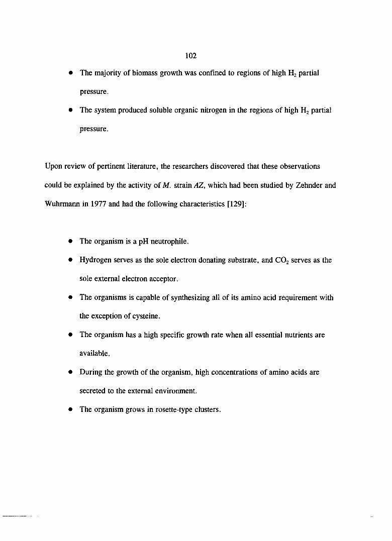
102
• The majority of biomass growth was confined to regions of high H2 partial
pressure.
• The system produced soluble organic nitrogen in the regions of high H2 partial
pressure.
Upon review of pertinent literature, the researchers discovered that these observations
could be explained by the activity of M. strain AZ, which had been studied by Zehnder and
Wuhrmann in 1977 and had the following characteristics [129]:
• The organism is a pH neutrophile.
• Hydrogen serves as the sole electron donating substrate, and CO2 serves as the
sole external electron acceptor.
• The organisms is capable of synthesizing all of its amino acid requirement with
the exception of cysteine.
• The organism has a high specific growth rate when all essential nutrients are
available.
• During the growth of the organism, high concentrations of amino acids are
secreted to the external environment.
• The organism grows in rosette-type clusters.

103
Sam-Soon et al. stated that the hydrogen partial pressure was the single-most important
variable in the granulation process, and that high H2 partial pressures stimulate the activity
of M. strain AZ. The researchers provided the following explanation for their hypothesis
[129, page 76]:
"When the M. strain/4Z is surrounded by excess substrate, i.e., high H2 partial pressure, the ATP/ADP ratio will be high. Simultaneously the high ATP level will stimulate amino acid production and cell growth. However, because M. strain AZ cannot manufacture the essential amino acid cysteine, cell synthesis will be limited by the rate of cysteine supply. If free and saline ammonia is present in excess there will be an over-production of the other amino acids; the organisms react to this situation by either releasing these excess amino acids to the surrounding medium and/or by linking these in polypeptide chains which it stores extracellularly by extrusion from active sites. These polypeptide chains bind species and other organisms into clusters forming a separate microbiological environment - the so-called biopellets."
The authors further state that granulation is unlikely in completely mixed systems due to
the usual low H2 partial pressure requirement for efficient methanogenesis. Granulation is
also unlikely in systems treating the following substrates:
• Acetate as sole substrate: methanogenesis from acetate as the sole substrate
does not produce Hj, and therefore will not stimulate M. strain AZ activity.
• Propionate as sole substrate: methanogenesis from propionate requires very
low H2 partial pressures.
• Fats and oils as substrate: Fats are broken down to volatile acids and
hydrogen only under low H2 partial pressures.

104
The best substrate for granulation was reported to be carbohydrates. These substrates
release hydrogen during breakdown to volatile acids under a wide range of Hj partial
pressures. Rapid acidogenesis of carbohydrates result in high H2 partial pressures and
stimulated, strain/4Zactivity.
The Spaghetti Theory. The "Spaghetti Theory" of granulation is based on the
presence of Methanothrix bacteria as the predominant acetoclastic methanogen [162].
Granulation develops when sufficient concentrations of Methanothrix are present in the
biomass. If present in low concentrations, conditions must be imposed on the system that
will select for Methanothrix, such as low acetate concentration. Upon selection for
Methanothrix bacteria, long filaments (up to 1,000 units long) will develop due to the
inherent nature of Methanothrix to form filamentous structures. After formation of the
initial Methanothrix clusters, full granulation of the biomass is stated to be inevitable.
Other bacteria are entrapped in the Methanothrix clusters, and the bacterial consortia
continue to grow and divide. Eventually, the aggregate will grow to sufficient sizes that
they are detectable as granules, consisting of a network of Methanothrix bacteria
interspersed with a variety of other bacteria [162].
Effect of Substrate and Temperature
Early investigations on granulation reported that the phenomenon was only
achievable when treating certain types of wastewaters, most notable soluble carbohydrate

105
wastewaters. Reports on temperature effects were also limited to mesophilic studies.
Since those early reports, granulation has been achieved in systems treating almost all
types of wastewaters at a range of temperatures (Table 11). Although granules have been
developed with a number of substrates, as Table 11 shows, granule stability may be
affected if the substrate is changed after granule development. For example, a granular
biomass developed on a sucrose wastewater may break apart upon changing to an acetic
acid wastewater. The granular biomass may also be inhibited by the new substrate and
Table 11. Substrates suitable for granule formation.
Substrate Reactor Type
Temperature CC) References
Volatile acid mixture EBR», UASB'' 30, 37, 39 16. 40, 167
Propionate UASB 35 41, 42, 74
Acetate EBR, UASB 30, 35 29, 38, 159
Methanol/N03' UASB 30 156
Sucrose UASB 30 139
Glucose EBR, UASB 30 8, 167, 171
Apple juice UASB 30 129, 160
Beet sugar EBR 33 71
Citrate UASB 35 165
Molasses UASB 35 165
Potato starch UASB 35 49, 109, 163
Maize processing UASB 35 124
Brewery UASB 34 51
Domestic sewage EBR 10, 20 71
* Expanded-bed or fluidized-bed reactor. '' Upflow anaerobic sludge blanket reactor.

106
simply not perform efficiently, with no obvious break-up of the granule [79, 104, 150,
166]. This phenomenon is explained by noting that various substrates inherently select for
specific bacterial species that are able to degrade the substrate. Therefore, a granule
grown on sucrose will contain a diverse consortia of acidogens, acetogens, and
methanogens. If this granular biomass is now used to treat acetic acid, the acidogens and
acetogens will not be able to survive, and may cause the granule to break apart due to cell
death and lysis.
However, some substrates appear to have no adverse effects on granule stability,
even though the granules were formed with a completely different wastewater. Granules
grown on non-fat dry milk have successfully been used to treat landfill leachate [60] and
starch wastewater [153]. Granules grown on propionate and then switched to pyruvate and
fiimarate were also reported to be stable (no granule disintegration) [62]. Numerous
examples exist of granules developed on a volatile acid mixture (acetic, propionic, and
butyric) successfully being used to treat a wide variety of industrial wastewaters,
including, potato starch, citric acid, sugar refinery, and meat processing [29, 78, 83, 133].
Effect of Chemical Enhancement
There are generally two mechanisms by which chemical enhancement may stimulate
the granulation process: chemical addition may form precipitates to which bacteria may
attach to form granules, or chemical addition may stimulate bacterial aggregation by
bringing the bacteria close together and linking the bacteria via salt bridges or by other

107
mechanisms. Although the precise mechanisms of enhancement is not always known,
several studies have investigated the effects of various metals, nutrients, and other elements
on the process of granulation [1, 33, 43, 44, 46, 67, 92, 103, 106, 160].
It has been hypothesized that some granules are formed via the attachment of
bacteria to inorganic precipitates present in the environment. These granules have an
inherent heavier specific gravity due to the inorganic precipitate, and, therefore, have a
higher settling velocity. These granules also have a high mechanical strength due to the
presence of the precipitate. Inorganic compounds that have been implicated in the
granulation process include precipitates of calcium (calcium carbonate, hydroxyapatite) and
sulfide precipitates (metal sulfides). Obviously, in an anaerobic wastewater treatment
system, other compounds and precipitates would also have an effect on granulation, but
these compounds have received special attention in the literature [1, 33, 43, 44, 46, 92].
Calcium and Phosphorous. In addition to calcium carbonate (CaCOj), which is
a common precipitate in alkaline waters containing calcium, hydroxyapatite may also
precipitate under various conditions. The formation of hydroxyapatite from calcium,
phosphorous, and the hydroxy 1 ion is shown in Equation 24 [98].
5Ca^' + ZPOl' + OH Ca^{PO;)pH\ (24)
An excess of calcium and phosphate is generally required for the precipitation of
hydroxyapatite to occur significant amounts. A high pH (> 8) is also necessary, although
108
hydroxyapatite will precipitate at lower pH levels provided the calcium and phosphates
concentrations are high [98]. Calcium has also been implicated in granulation through its
stabilizing effect on the generally negatively-charged bacterial surface. Calcium has been
shown to stabilize carboxyl groups and other negatively charged groups on extracellular
biopolymers, and actually allow separated bacteria to come closer together. It has been
suggested that the Ca^^ may act as a bridge between different biopolymers, thus,
effectively joining two bacteria. Subsequent aggregation of more bacteria could lead to
granulation [1, 43, 46, 92].
The effect of calcium and phosphorous concentration has been the focus of several
investigations concerning granulation. Alibhai and Forster [1] reported that calcium and
phosphorous stimulated the granulation process in UASB reactors at concentrations of 80
and 190 mg/L, respectively. Other multivalent cations, such as aluminum and silicon,
were also observed in relatively high concentrations within the granule, suggesting that
these elements may be important in granulation as well. Hulshoff Pol et al. [67] reported
that moderate Ca^"^ concentrations may enhance granulation, but that very low or very high
Ca^^ concentrations appear to inhibit granule formation. UASB reactors treating a volatile
acid wastewater were supplemented with Ca^^ at 6, 150, and 450 mg/L. The Ca^^
concentration of 150 mg/L was observed to enhance granule development the most rapidly.
Mahoney et al. [92] reported that 100 mg/L of Ca^^ enhanced the formation and
settleability of granules. The researchers studied the effect of calcium using two UASB
reactors treating a mixture of volatile acids. One of the UASBs received 100 mg/L of

109
in addition to the substrate feed (calcium positive reactor), and the other UASB
received no additional Ca^"^ (control). Although granulation was observed in both of the
UASB reactors, the calcium positive UASB granulated more rapidly than the control
UASB. In addition, the granules that developed in the calcium-positive UASB had settling
velocities that were 3 to 4 times faster than the granules that developed in the control
reactor. Guiot et al. [44] reported that Ca^^ did not enhance the formation of granules.
However, exposure of the granules to Ca^^ did improve their settleability, presumably due
to incorporation of calcium precipitates which subsequently increased the granules' specific
gravity [46].
One study designed to define the requirement for calcium and phosphorous utilized
ethylene glycol-bis(p-aminoethyl ether)-N,N-tetraacetic acid (EGTA) as a calcium-specific
chelant [43]. Upon treatment of granules with EGTA, the calcium and phosphorous
concentrations of the granules subsequently decreased, and disintegration of the granules
also occurred to varying extents. Additionally, the molar ratio of phosphorous to calcium
(P/Ca) lost from the granules was approximately 0.59, which is very close to the P/Ca
ratio of hydroxyapatite (P/Ca = 0.625). These observations suggested the importance of
calcium and phosphorous precipitation (as hydroxyapatite) to the granulation process [43].
Iron. Nickel. Cobalt, and Other Heavv Metals. Although the beneficial effects
of heavy metals on the biochemical aspects of methanogenesis have been well documented
[106, 142], heavy metal precipitates may also play an important in the granulation process

110
of flocculent anaerobic biomass. The heavy metals precipitate in the presence of alkalinity
and sulfide to form metal carbonates and metal sulfides, respectively (Equations 25 and
26). Hydroxide precipitates may also be formed, but these are normally only significant at
high pH levels (Equation 27).
M e + COj' ^ MeCOj I (25)
+ S^- ^ MeS I (26)
+ 20H- Me{0H)2 J (27)
In Equations 25 through 27, "Me" represents any divalent heavy metal. In many anaerobic
applications, sulfate is present in the influent wastewater. The sulfate is quickly reduced to
sulfide by the sulfate-reducing bacteria, and these sulfides are then available to precipitate
heavy metals. The solubility products of metal sulfides and other metal precipitates are
extremely low (Table 12). Therefore, precipitation of the metal is very slowly reversible,
and the majority of a metal will be present as metal sulfide, with smaller amounts of metal
carbonates and hydroxides. The metal precipitates may act as granulation nuclei, similarly
to the proposed mechanisms for hydroxyapatite [33].
Iron is normally the most abundant heavy metal in anaerobic treatment systems.
Early reports [126, 138] on the effect of ferric chloride on sewage digestion indicated that

FeClj concentrations in excess of 5 to 10 mg/L retarded methanogenesis and may be toxic
to anaerobic bacteria. Later reports on the effect of iron reported that high iron
concentrations may be inhibitory, but that the inhibition was mainly due to precipitation of
iron with phosphate, resulting in limiting soluble phosphorous levels in the digester [115].
Another inhibitory effect of Fe^^ on anaerobic digestion results from the competing
Table 12. Solubility products of metal salts [98]. Metal Precipitate Solubility product, Kj pK.
AgzCOj 3.0 x (10)-'' 11.5
CdCOj 5.0 x (10)-'^ 11.3
ZnCOa 6.0 X (10)-" 10.2
FeCOj 3.0 X (10)-" 10.5
PbC03 1.5 X (10)-'3 12.8
CU2C03(0H)2 1.6 xdO)-'" 33.8
CU3(C03)2(0H)2 l.Ox(lO)-'^ 46.0
AgaS 1.0 X (10)-^^ 49.0
CuS 4.0 X (10)-^® 35.4
CujS 1.0 X (10)-^® 48.0
PbS 1.0x(10)-2« 28.0
CdS l.Ox (10)-2® 26.0
ZnS 1.0x(10)-2^ 24.0
NiS 1.0x(10)-2'» 24.0
FeS 1.0x(10)-'» 18.0

112
reactions of the iron reducing bacteria. Under appropriate conditions, the iron reducing
bacteria may out-compete the methanogens, resulting in reduced methane production [117].
Still later reports [58] indicate that moderate levels of iron (10 to 120 mg/L) stimulate
methanogenesis. These investigations reported significant iron precipitation during
digestion, but did not indicate that the precipitates affected the digestion process either
positively or negatively.
X-ray analysis of granular biomass normally results in significant quantities of
ferrous sulfide and ferrous carbonate. Ferrous sulfide is often present in sufficient
quantities in granules that gives the entire granule a characteristic black color, and can
constitute over 30% of the ash fraction of a granule [33]. This and other more recent
studies indicate that iron precipitates may stimulate the adhesion of bacteria and the start of
granulation [32, 33].
Biopolymers. Extracellular biopolymers have been briefly discussed in relation
to their role in granulation. Most reports indicate that granular biomass normally contains
a significant amount of extracellular polysaccharides, proteins, and lipids. This
extracellular material may only comprise from 1 to 10% of the dry weight of the granule,
but it has been suggested that it plays a role in stabilizing and strengthening the granule
structure. The stabilization results from the numerous functional groups on the
biopolymers which are capable of interacting with other biopolymers and ions. The

113
network formed by the polymers and ions could provide additional mechanical strength
[33, 103, 130].
Morgan et al. [103] investigated the effect adding biopolymers to a UASB reactor.
It was believed that the addition of biopolymers, which were extracted from granular
biomass, would enhance the granulation process of a non-granular biomass. The results
from this experiment indicated that initiation of granulation could be enhanced with
biopolymers. However, inhibition of the UASB with respect to COD removal was also
apparent with the addition of biopolymers. This latter effect was not understood by the
researchers [103]
Effect of Physical Enhancement
The enhancement of granulation through physical methods, such as the addition of
an attachment matrix, is the ftmdamental basis behind the expanded-bed reactor system.
The basic principle is that bacteria will attach to and grow on a support matrix (e.g., sand
or GAC) and form granules over time. Alternatively, granular biomass may be used as a
portion of the seed sludge in almost any anaerobic treatment system to enhance reactor
start-up.
Morgan et al. [103] reported that the addition of GAC and granular biomass (in
separate experiments) to UASB reactors significantly enhanced the formation of a fully-
granular biomass. Wang et al. [159] and Fox et al. [38] reported on the formation of
granules in expanded-bed reactors using GAC as the support media. The formation of

114
granules of up to 5 mm in diameter was reported. An additional benefit to using GAC was
cited as the adsorption capacity of the GAC. GAC is able to adsorb soluble substrates,
thus providing an advantageous location for bacterial attachment and subsequent growth.
Other attachment media have also been used to promote granulation. Fox et al.
[38], Gorris and van Deursen [40], and Ashikago et al. [5] used silica sand (average
diameter = 0.3 to 0.7 nmi) in expanded-bed reactors. Bacterial attachment and
granulation was induced in these systems within 50 to 60 days, with granule diameters
reported in the range of 0.7 to 5 mm. The small crevices of the sand particles were the
first areas to be colonized, with subsequent growth of the granule developing outward from
the crevices. Sand was reported to be less efficient than GAC for granule formation.
Powdered zeolite with a diameter of 50 to 100 /xm has also been shown to enhance
granulation in expanded-bed reactors [167]. Most of the biomass in these experiments
existed as a thin film on the carrier with diameters less than 0.25 mm. However, other
particles were also present with diameters of over 1 mm, indicating significant growth of
the biomass attached to the carrier. Other attachment media that have been successfully
used include anthracite and polyvinyl chloride (PVC) particles [38, 71].

115
EXPERIMENTAL SETUP
Four identical reactor systems, each consisting of one ASBR, a substrate feed
system, an effluent decant system, a gas mixing system, and a gas measuring system, were
used for the experiments in this research. The ASBRs were constructed at the Engineering
Research Institute Machine Shop at Iowa State University. Excessory materials, such as
tubing, clamps, fittings, and connections, were purchased at the Chemistry Stores and
Central stores, also located at Iowa State University. Additional equipment and materials
were purchased as noted below. The reactor systems were housed in a constant
temperature room which was kept at SS^C ± 0.5°C for the duration of the experiments.
The entire system for one of the identical units is shown in Figure 15.
Anaerobic Sequencing Batch Reactor Design
The body of the four identical ASBRs (Figure 15) were constructed of !4-in thick
Plexiglas. The reactors were cylindrical, with an inside diameter of 5.5 in, an outside
diameter of 6 in, and a total depth of 37 in. The total volume of each ASBR was
approximately 14 liters. The top and bottom of the cylindrical tube were flanged with an
outside flange diameter of 9 in. Nine-inch diameter round plates ('/2-in thick) were
fastened to the top and bottom flanges with 12 equally-spaced 1/2-in bolts (1 '/2-in long). A
rubber gasket was placed between the plates and the flanges to provide an air-tight seal
(Figure 16). Nine side ports were equally-spaced down the side of the ASBR. These 1 VA-
in Plexiglas ports (3/8-in diameter) extended through to the inside of the ASBR and

116
Recirculated Biogas Aspirator
Bottle
Foam
Biogas Out
ASBR
DifTuser
Gas Sampling
Port
Biogas Out
Port / / (/ Iron Oxide Scrubber
Water Observation
Bottle
Polymer Solution
Effluent
Pump)— Influent
Figure 15. Anaerobic sequencing batch reactor setup.

117
ASBR
5/8-in Diffuser
12 1/2-in holes for 1.5-in bolts
O o o 3/8-in Biogas port
3/8-in Biogas port
Nut and Bolt 1/2-in diameter 1.5-in long
Figure 16. Scliematic of the top cover of the ASBR.

118
extended 1.0 in on the outside (Figure 15). Each of the ports was connected to a 6-in long
piece of 3/8-in diameter Nalgene tubing (Sybron Corporation, Rochester, NY), which was
clamped to provide an air tight seal. The bottom port was connected to the substrate feed
pump, and one of the upper ports was connected to the effluent decant pump. The decant
port was selected based on the HRT of the system. As the HRT was increased, a lower
port was used for decanting due to the larger volume of liquid that was required to be
decanted each cycle.
The top plate on the ASBR contained two additional ports identical to those
described above. One port served as the biogas outlet from the ASBR, and the other
served as a liquid and foam return inlet to the ASBR. These ports are described later in
the section on gas/foam separation. A third port was located in the top plate for biogas
recirculation and is described in the biogas mixing section (Figures 15 and 16).
Gas/Foam Separation System
Biogas exiting the ASBR through the middle top port (Figure 16) was directed to
the gas/foam separation bottle, which had a volume of approximately 3 liters (Figure 15).
Under normal conditions, the separation bottle served no function. However, under
conditions of excessive foaming, some foam left the ASBR in the biogas outlet port and
was collected in the gas/foam separation bottle. This bottle contained three ports in the top
rubber stopper and an additional port at the bottom. The ports in the stopper
consisted of 1/4-in glass tubes, which extended from 1.5 in above the stopper to several

119
inches below the stopper. One of the ports was used as the biogas inlet (from the ASBR),
one served as the biogas outlet (to the gas measuring system), and one served as a biogas
outlet during biogas recirculation. Foam entering the bottle fell to the bottom and was
returned via the bottom port to the ASBR. Tubing that connected the gas/foam separation
bottle with other parts of the system was 3/8-in in diameter.
Biogas Recirculation System
Mixing was accomplished by recirculating the biogas in a closed loop to the bottom
of the ASBR through a stainless steel ring difftiser system. The difftiser system consisted
of a 5/8-in diameter pipe which extended from the bottom of the ASBR through the top
plate to 2-in above the top of the ASBR. The pipe was positioned along the edge of the
ASBR so that at the bottom of the pipe a 1/4-in ring difftiser could be attached (Figure 15).
The difftiser consisted of two concentric rings connected by three stainless steel tubes. The
inner and outer rings were 4V2-in and 2'/2-in in diameter, respectively (Figure 17). The
inner ring had six 1/32-in equally-spaced holes and the outer ring had eight 1/32-in equally
spaced hole drilled in the bottom to provide the outlet of the difftisers for mixing. All
parts of the diffuser system were hollow to allow the recirculated biogas to flow through
them.
The recirculation system worked as follows; Biogas produced from methanogenic
activity exited the ASBR through a port described earlier and was discharged to the
gas/foam separation bottle. When the ASBR was mixed, a peristaltic pump turned on and

120
ASBR
Diffuser Ring
DifTuser Tube
Stainless Steel Tubing 1/4-in O.D.
Drilled Holes on Bottom of Diffuser
1/32 in
DriUed Holes 1/32 in
4.9 in
Diffuser Tube Connection
Figure 17. ASBR biogas recirculation diffuser system.

121
pulled biogas out of the gas/foam separation bottle via one of the top ports. The discharge
end of the pump was connected with 5/8-in Nalgene tubing to the stainless steel diffuser
pipe. The biogas discharged through the ring diffiisers and rose to the surface of the
ASBR, thereby mixing the system and completing the biogas loop.
The pump used for biogas recirculation was a 50-600 rpm variable speed peristaltic
pump with a size 18 pump head (both from Cole-Parmer Instrument Company, Chicago,
IL). The recirculation pumps were connected to a model XT Chrontrol timer (Chrontrol
Corporation, San Diego, CA) which turned the gas pumps on and off at programmed
times. The pump head tubing was Masterflex size 18 Norprene tubing (Cole-Parmer
Instrument Company, Niles, IL). The connections between the pump tubing and the inlet
and outlet tubing were 2-way, 1/4 to 5/8-in polyethylene connectors (Chemistry Stores,
Iowa State University, Ames, lA).
Biogas Collection and Measurement System
The biogas that was produced ultimately left the gas/foam separation bottle via the
gas exit port to the gas measurement system (Figure 15). The gas exit port was connected
to a water observation bottle (one-liter volume) with 3/8-in Nalgene mbing. The
observation bottle had a rubber stopper with inlet and outlet glass tubes extending out the
top and bottom of the stopper. The inlet glass tube extended 1/2-in below the water level
in the bottle so that bubbles of gas could be visually observed. There were two valves
between the gas/foam separation bottle and the observation bottle. The first valve was a
122
three-way T-connection that was connected with the tubing to the gas/foam separation
bottle, the observation bottle, and also to a gas bag which had a volume of four liters. The
bag served as a reservoir of gas and provided gas to the ASBR (by deflating) during
decanting to avoid drawing a vacuum on the system. Just before the observation bottle was
a one-way check valve, the purpose of which was to prevent gas being drawn back through
the observation bottle (and downstream equipment) during decanting.
A hydrogen sulfide scrubber (one-liter volume) containing sponges soaked in a
solution of ferric oxide was placed after the observation bottle. The inlet and outlet from
the scrubber were identical to the observation bottle, with the exception that there was no
water in the scrubber. Hydrogen sulfide produced in the ASBR was removed from the gas
stream by reaction with the ferric oxide to form ferrous sulfide, which formed a black
precipitate in the scrubber bottle.
After the scrubber bottle, the gas passed through a cylindrical blown-glass gas
sampling compartment (4-in long and 1-in diameter) which had a 'i-in port with a rubber
septum placed snugly into it (Figure 15). This compartment was used to sample the biogas
with a syringe for gas composition analyses using chromatography.
The final stage of the biogas collection system was the gas meter. After exiting the
gas sampling compartment, the biogas entered a wet-test gas meter (Precision Scientific,
Inc., Chicago, IL), which measured the volume of biogas produced over time. The gas
was vented to the buildings air ventilation system. All tubing used in the gas collection
and measurement system was Nalgene brand tubing with an inside diameter of 3/8 in and

123
a wall thickness of 1/16 in. Appropriate connectors were placed between all parts of the
system so that any one component could be taken out and repaired without disrupting the
flow of biogas.
Substrate Feed and Effluent Decant Systems
The substrate used in the experiments was prepared daily (described in the
Experimental Procedures section) in 20-liter polyethylene carboys. Each carboy was
placed on a magnetic stirring plate (Model PC-310 Laboratory Stirrer, Corning Inc.,
Corning, NY), and a 2-in magnetic stir bar was placed in the carboy. The magnetic stir
plates were connected to a Chrontrol timer which mrned the magnetic stir plates on and off
during the feed cycle. A 6-in section of 3/8-in glass mbing was connected with 3/8-in
Nalgene mbing to the substrate feed pump. The glass end was inserted into the carboy
while the other end of the tubing was connected to the pump head tubing in an identical
fashion, as earlier described. The pumps were 60-rpm constant speed peristaltic pumps
(Cole-Parmer Instrument Company, Chicago, IL) and were connected to a Chrontrol timer
which turned them on and off at the appropriate time. The discharge end of the pump was
connected with 3/8-in Nalgene mbing to the bottom side port of the ASBR.
The decanting pumps, timer, and mbing were identical to those used for the
substrate feed system. The selected side port for decanting was connected to the decant
pump, which discharged the effluent to a sanitary sewer drain.
124
Coagulant Feed System
In experiments where coagulant was added to the ASBR for granulation
enhancement, additional equipment was necessary. The coagulant feed system consisted of
a 2-liter polyethylene bottle, which contained the respective coagulant for that experiment.
A 1/8-in polyethylene Nalgene tube was inserted into the container and connected to a
variable speed peristaltic pump with a size 16 pump head (Cole-Parmer). The pump head
tubing was also 1/8-in Nalgene tubing. The pump outlet was cormected with 1/4-in
Nalgene tubing to a three-way T-connection in the ASBR foam return line. The pump was
controlled by a Chrontrol timer which turned the pump on for one minute during the last
mixing cycle just prior to the settle phase of the ASBR cycle (Figure 15).

125
EXPERIMENTAL PROCEDURES
Substrate Feed Preparation
The substrates used in this study were prepared daily to minimize biological
degradation of the feed while it sat in the feed carboys. Sucrose (Chemistry Stores, ISU)
was the main substrate (carbon and energy source) used. As stated in the Literature
Review section, soluble carbohydrates have been cited as the best substrate to achieve
granulation in UASB reactors. For this reason, sucrose was chosen as the primary
substrate in most of the experiments. Since pure sucrose does not contain nitrogen or
other essential nutrients and trace metals, addition of these other elements were necessary.
Nitrogen was added as ammonium hydroxide, potassium and phosphorous as potassium
phosphate (dibasic), and other trace metals as chloride salts. Additionally, alkalinity was
added to the feed solutions in the form of sodium bicarbonate. Table 13 lists the recipe
used for the sucrose experiments. COD, nitrogen, and phosphorous were added in a
100:5:1 ratio for all experiments. A review of the literature for similar experiments
indicated that this ratio was common and provided a suitable environment for anaerobic
biological degradation. Although the nitrogen added was in excess of that required for
biomass synthesis, the additional nitrogen provided a source of alkalinity and buffering
capacity in the ASBRs.
A second substrate was used in later experiments to determine if previous results
could be attributed to the substrate employed. This latter substrate was a mixture of a
food-grade beef extract soup base (Kraft, Inc., Glenview, IL) and glucose (Chemistry

126
Stores, ISU). The two substrates were blended in tap water with a warring blender in a
mixture that contained a 1:1 ratio of COD from each substrate. Table 14 outlines the
recipe used for the beef/glucose experiments. Table 15 lists the composition of the beef
extract obtained from the Kraft Company.
One obvious difference between the two substrates was the fact that the
beef/glucose feed solution contained a relatively large amount of fat, whereas the sucrose
solution contained essentially zero fat. This difference became the source of some
operational difficulties due to the hydrophobic nature and density of fat. The fat tended to
Table 13. Sucrose feed mixture.
Component Amount Added
(per gram of feed COD)
Sucrose, mg
Nitrogen, mg
Phosphorous, mg
Iron, mg
Manganese, mg
Cobalt, mg
Nickel, mg
Zinc, mg
Molybdenum, mg
Copper, mg
Boron, mg
Bicarbonate, g/L as CaCOj'
960.00
50.00
10.00
0.05
0.02
0.02
0.06
0.08
0.06
0.31
2.40
1.25
* Alkalinity was directly added at the rate of 4 grams of NaHCOj per liter of feed.

127
form a layer on the top of the feed carboys, as well as in the reactors. This observation is
dealt with in more detail later. A second difference between the two substrates was that
the beef also contained protein, which became an additional source of nitrogen and sulftir.
Since the feed solutions were prepared daily, stock solutions of the nutrients
(termed the NPK solution) and trace metals were prepared and stored as aqueous solutions.
Tables 16 and 17 list the composition of the nutrient solution and trace metal solution,
respectively.
Table 14. Beef extract and glucose feed mixture.
Component Amount Added
(per gram of feed COD)
Beef extract, mg
Glucose, mg
Nitrogen, mg
Phosphorous, mg
Iron, mg
Manganese, mg
Cobalt, mg
Nickel, mg
Zinc, mg
Molybdenum, mg
Copper, mg
Boron, mg
Bicarbonate, g/L as CaCO
480.00
860.00
50.00
10.00
0.05
0.06
0.08
0.31
2.00
0.06
0.02
0.02
1.25
Alkalinity was directly added at the rate of 3.3 grams of NaHCO, per liter of feed.

128
Table 15. Composition of the beef extract soup base. Amount
Component (% by weight)
Hydrolyzed vegetable protein 12.9
Fat 13.5
Carbohydrates 24.0
Sodium 18.1
Potassium 8.8
Table 16. Nutrient (NPK) solution." Concentration
Component (g/L)
Potassium phosphate, dibasic 68.8 Potassium 30.9 Phosphorous 12.2
Ammonium hydroxide 148.1 Ammonia 74.1 Nitrogen 61.0
• Added 0.886 mL of this solution per gram of COD.
The sucrose solution was prepared as follows. A measured amount of sucrose
(based on the COD loading) was added to approximately 1 liter of warm tap water. This
mixture was placed on a magnetic stir plate until all of the sucrose had dissolved. This
mixture was then poured into the 20-liter feed carboy. Sodium bicarbonate was weighed
and poured into the carboy. An appropriate amount of the NPK solution was then
measured with a volumetric cylinder and an appropriate volume of the trace metal solution

129
Table 17. Trace metal solution/
Element Compound Concentration of Element
(g/L)
Iron FeCl2- 4H2O 14.00
Manganese MnCl2- H2O 3.50
Cobalt CoCl2- 4H2O 0.93
Nickel NiClz- 4H2O 0.62
Zinc ZnCl2 0.60
Molybdenum (NH4)6M07024- 4H2O 0.68
Copper CuClj- 4H2O 0.28
Boron HBO3 0.22
* Added 0.089 mL of this solution per gram of COD.
was added with a syringe. Warm tap water was then added and the volume of the feed
solution was adjusted to the appropriate level, depending on the HRT of the system.
The beef/glucose feed mixture was prepared similarly. The beef extract and
glucose were weighed on a balance and then placed in a warring blender along with two
liters of hot tap water. Hot water was used since it tended to keep the fat in solution better
than cold water. The warring blender was mrned on for one or two minutes, and then the
contents were poured into the feed carboy. The other ingredients were added as before.
The feed carboys were then taken to the controlled-temperature room in which the reactor
systems were housed, placed on the magnetic stir plates, and a magnetic stir bar was
placed in each carboy. The feed lines to the ASBRs were inserted into their respective
carboys and the fed preparation was then completed. The volume of feed substrate

130
prepared was 2 liters in excess of the amount fed to the ASBRs on a daily basis. This was
done to ensure that air would not be pumped in to the reactors, which would occur if the
carboys were completely empty. The remaining two liters were poured down the drain
prior to making the new feeds, and the carboys were cleaned and rinsed to avoid bacteria
growth.
Tap water was used in place of distilled or deionized water for two reasons. First,
the logistics of the distilled water system in the environmental engineering laboratory were
such that a relatively long period of time would be required to obtained sufficient distilled
water to make all of the substrate feeds. Second, the tap water provided other essential
nutrients for the biological systems, most notably, calcium, magnesium, and sulfur
(sulfate). The average composition of the Ames' tap water is shown in Table 18.
Biological Seeding of the ASBR
Because of the nature of the experiments in this study, it was necessary to re-start
the ASBRs with new biological seed every 2 to 5 months. Each time the ASBRs were re
started, the existing biomass in the reactors were emptied into carboys, and the reactors,
diffusers, ports, and tubing were thoroughly cleaned. New anaerobic biological seed was
obtained from the primary anaerobic digesters at the City of Ames Water Pollution Control
Plant. The seed was brought back to the environmental engineering laboratory and sieved
with a 1 mm screen to remove large particles, hair, gum, and other objects which
inevitably become part of the anaerobic digester contents. The large particles removed

131
Table 18. Ames municipal water analysis. Average Concentration
Component (mg/L)
Calcium, as Ca 130-- 140
Magnesium, as Mg 20-•30
Sulfate, as S04^" 70--90
Iron, as Fe 0 .09-•0 .11
Carbonate hardness, as CaCOj 40-•60
Noncarbonate hardness, as CaCOs 120-• 130
Alkalinity, as CaCO^ 40- 60
pH" 9 .4-•9 .7
' pH is reponed as pH units.
were discarded and the sieved seed was then placed into carboys and purged with methane
gas to remove any entrained oxygen. The ASBRs were also purged with methane, after
which the seed was pumped into the sealed ASBRs. Approximately 8 to 10 liters of the
seed (depending on the solids content of the seed) were pumped into each reactor, and then
the liquid volume of the ASBR was adjusted to 11 liters with tap water. The liquid volume
was subsequently adjusted to 12 liters with the addition of 1 liter of a substrate solution
(described below). Each ASBR had a total volume of 14 liters with a 2-liter headspace.
As stated, the amount of seed added to the ASBRs was dependent on the solids
concentration of the seed material. The suspended solids concentration of the seed material
was generally about 30,000 mg/L, although this varied each time new seed was obtained
from the treatment plant. The target MLSS concentration in the reactor (liquid volume of
12 liters) was between 20,000-25,000 mg/L.

132
During and after seeding, the ASBRs were purged with methane to remove all of
the oxygen from the system. Gas chromatography was used to determine the approximate
oxygen composition of the gas in the reactor, and methane purging was continued until the
oxygen peak was diminished to below detectable levels (O2 < 1 % of gas). Methane
purging was then stopped. The ASBRs were then fed with 1 liter of the respective
substrate solutions and the gas meter readings were recorded. At this point, the
experiment was considered started.
ASBR Start-up and Operation
Each of the ASBRs was operated independently of the other ASBRs during the
experiments. The operational characteristics of the ASBR were presented earlier in the
Literature Review section. The ASBRs were always operated with a cycle length of six
hours, corresponding to four cycles per day. The only exception to this was during the
first one or two days of operation in which the ASBRs were operated with only two cycles
per day to avoid loss of too much biomass. Generally, two HRTs were used throughout
the study, 48 and 24 hours. After initial start-up, the ASBRs were operated at a 48-hr
HRT and a COD load of 2 g/L/day until the system began to settle well. When settling
was stable and clear supernatant was apparent, the HRT of the system was decreased to 24
hrs by doubling the amount fed and decanted each cycle while maintaining the COD load at
2 g/L/day. The COD load was kept constant by diluting the feed substrate. The decision
of when to decrease the HRT was not always clear-cut, and factors such as COD removal

133
efficiency were also taken into consideration. For the majority of the tests, the ASBRs
were operated at a 48-hr HRT for at least 20 to 25 days, although this varied considerably
among the individual experiments.
The pumps used for feeding and decanting were constant-speed peristaltic pumps
(previously described). Therefore, in order to achieve the desired feeding and decanting
volumes, the feed, decant, settle, and react phases of the ASBR cycle were changed
accordingly (Table 19). It was desired to decrease the HRT of the system as quickly as
Table 19. ASBR cycle time for 48 and 24-hr HRTs. Time per cycle, hrs (min)
Phase 48-hr HRT 24-hr HRT
Feed 0.13 (8) 0.26 (16) React 4.96 (297) 4.83 (289) Settle 0.78 (47) 0.65 (39) Decant 0.13 (8) 0.26 (16)
Total 6.00 (360) 6.00 (360)
possible. It was hypothesized that increasing the hydraulic pressure would increase the
rate at which the biomass formed granules. Similarly, increasing the COD load as quickly
as possible was also thought to be beneficial for granulation. Increasing the COD load
provided more substrate, which, if biologically degraded, would produce more viable
biomass. Increasing the COD load also resulted in more internal mixing due to higher

134
biogas production rates, which tended to carry lighter biomass particle upward while the
heavier particles were still able to settle sufficiently.
The ASBRs were operated according to the times in Table 19 for all experiments.
Termination of an experiment occurred after granulation of the biomass occurred or when
it was determined (by objective and subjective analyses) that granulation would not occur
within a reasonable period of time. In the experiments in which the biomass did granulate,
it was normally apparent that granulation would occur within approximately one or two
months of operation. Although physical granulation may not have been apparent within
this time frame, the biomass generally appeared slightly different than in the ASBRs that
did not granulate at all, and reactor performance based on COD removal was generally
better at an early stage as compared to the granule-negative experiments.
It is noted here that the ASBRs in these experiments were seldom operating under
equilibrium conditions. That is, in most of the studies under Dr. Dague's supervision, the
systems are operated under specified conditions for a period of time so as to establish
equilibrium, or at least pseudo-equilibrium based on a relatively constant daily methane
production and COD removal at a given COD loading rate over a period of several HRTs.
The experiments in this study, however, were very time-dependent. It was deemed
beneficial to the granulation process to increase COD and hydraulic pressure as quickly as
possible without deterioration of the system. Therefore, the systems were seldom
operating under equilibrium conditions for any significant period of time. Rather, after an
increase in the COD was affected, the systems were given time to adjust to the new

135
conditions, and, if the overall efficiency of the system remained approximately the same or
increased, the COD loading rate was again increased. Of course, data were collected at
each COD loading rate so that removal efficiencies, MLSS, and other pertinent operational
parameters could be monitored over the entire course of an experiment.
The overall effect that this had on the data was to underestimate the COD removal
efficiency and MLSS values at any given conditions. For instance, if the COD loading rate
on a given ASBR was increased from 3 to 4 g/L/day, and the system immediately adjusted
to this increase through increased gas production, the COD loading rate was subsequently
increased to a higher value in a short time period. The alternative to this would have been
to maintain the ASBR at 4 g COD/L/day for a period of 3 or 4 weeks, during which time
the COD removal efficiency would have increased to a higher level and the MLSS
concentration also would have increased to near equilibrium values for that loading rate.
As previously stated, the basis for the rapid increase in loading rate was to put pressure on
the system to select for the most active, best-settling biomass, thereby enhancing conditions
for granulation.
ASBR Mixing
Mixing of the ASBR was conducted on an intermittent basis throughout the study.
During the feeding phase of the cycle, the gas recirculation mixers were turned on to
achieve intimate mixing between the substrate and the biomass. The mixers were turned
on for three minutes every 30 minutes during the react phase to release any entrapped gas

136
bubbles within the ASBR and to provide contact between the substrate and biomass.
Mixing was not performed during the last 30-minute period of a cycle. That is, if the
decant phase was to begin at 2:45, the last mixing cycle would occur at 2:00. The mixers
would be shut off from 2:03 to 2:45, which defined the settle phase. Of course, the mixers
were also off during the decant phase, which immediately follows the settle phase.
The mixing intensity was maintained at a maximum velocity gradient, G, of 100/sec
and a minimum of 50/sec. This was accomplished by adjusting the speed control on the
variable speed gas recirculation pump.
Granulation Enhancement
Attachment Matrices
Various attachment matrices were used to enhance granulation throughout this study
(Table 20). The attachment matrices were added only once at the beginning of each
experiment. Although it was physically impossible to determine whether the biomass
actually attached to the matrices, performance and the on-set of granulation were compared
to control reactors in which no attachment matrices were added. Preliminary experiments
with only tap water and each attachment matrix were performed to indicate the degree to
which the attachment matrices could be suspended during mixing of the ASBR. If the
matrix settled to the bottom of the ASBR and did not mix thoroughly with the reactor
contents, it was of little use for granulation enhancement. As expected, all of the matrices
employed in this study were easily suspended from the bottom of the ASBR during mixing.

137
The matrices used in these experiments included powdered activated carbon (PAC),
granular activated carbon (GAC), garnet sand, and silica sand. It was expected that the
two activated carbons would enhance overall performance of the ASBR by supplying a
form of buffer capacity to the ASBR. The adsorption capacity of the carbon would, in
effect, store COD in the reactor, which could then be utilized by the biomass as needed.
The adsorption capacity of the activated carbons was also expected to provide suitable
attachment sites for the bacteria. The two types of sand were used to compare the effect of
adsorption on reactor performance and granulation enhancement. Sand is also generally
less expensive than activated carbon. Therefore, if the two types of matrices performed
equally well, sand would be a better economic selection.
Preliminary experiments with PAC were conducted to determine the optimum
concentration of attachment matrix to add at the start of the granulation experiments. The
four ASBRs were seeded with municipal digester biosolids and four different
concentrations of PAC were added; 500 mg/L, 1,000 mg/L, 2,000 mg/L, and 5,000
mg/L. Based on overal ASBR performance (COD removal, settling characteristics, etc.)
over the first 40 days of operation, the value of 2,000 mg/L of PAC was selected for
additional experimentation. This concentration was also used in latrer experiments with
GAC, silica sand, and garnet. The attachment matrices were weighed on a digital scale
and then injected into one of the top ports of the ASBR during mixing on day zero. After
this day, additional matrix material was not added to any of the ASBRs.
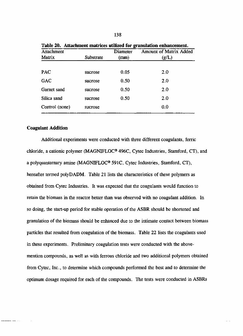
138
Table 20. Attachment matrices utilized for granulation enhancement. Attachment Matrix Substrate
Diameter (mm)
Amount of Matrix Added (g/L)
PAC sucrose 0.05 2.0
GAC sucrose 0.50 2.0
Garnet sand sucrose 0.50 2.0
Silica sand sucrose 0.50 2.0
Control (none) sucrose 0.0
Coagulant Addition
Additional experiments were conducted with three different coagulants, ferric
chloride, a cationic polymer (MAGNIFLOC® 496C, Cytec Industries, Stamford, CT), and
a polyquanternary amine (MAGNIFLOC® 591C, Cytec Industries, Stamford, CT),
hereafter termed polyDADM. Table 21 lists the characteristics of these polymers as
obtained from Cytec Industries. It was expected that the coagulants would function to
retain the biomass in the reactor better than was observed with no coagulant addition. In
so doing, the start-up period for stable operation of the ASBR should be shortened and
granulation of the biomass should be enhanced due to the intimate contact between biomass
particles that resulted from coagulation of the biomass. Table 22 lists the coagulants used
in these experiments. Preliminary coagulation tests were conducted with the above-
mention compounds, as well as with ferrous chloride and two additional polymers obtained
from Cytec, Inc., to determine which compounds performed the best and to determine the
optimum dosage required for each of the compounds. The tests were conducted in ASBRs

139
Table 21. Polymer characteristics. Parameter MAGNIFLOC® 496C MAGNIFLOC® 591C
Type
Charge
Polymer type
Chemical make-up
Polymer solids
BODj"
COD^
dry powder
strongly cationic
co-polymer
acrylimide
acryloyloxyethyltrimethyl-
ammonium chloride
85%
400 mg/L
4,500 mg/L
liquid
moderately cationic
homopolymer
dialyldimethylammonium
chloride
55%
310 mg/L
2,250 mg/L
Based on a 1 % solution.
Table 22. Coagulants utilized for granulation enhancement. Coagulant Dosage Added Substrate (mg/L/cycle)
Ferric Chloride sucrose 5 to 10"
Cationic (496C) sucrose 1
Cationic (496C) beef/glucose 1
PolyDADM (59IC) sucrose 2 to 5
Control sucrose 0
Control beef/glucose 0
' The dosage of ferric chloride is reported as mg/L as Fe.

140
that had been operating in previous experiments that had been discontinued. Ferrous
chloride and the additional two polymers did not achieve acceptable coagulation at any of
the dosages examined, and were, therefore, not used in subsequent experiments. Ferric
chloride performed well at dosages of 5 to 10 mg/L (as Fe), the cationic polymer
performed well at dosages as low as 1 mg/L, and the polyDADM coagulant performed
well at dosage of 5 to 10 mg/L.
Addition of coagulants began on day zero of the experiments. The coagulant was
added once per cycle during the last mixing period of the cycle, just before the settling
phase. The coagulants were added with a peristaltic pump (described earlier) for a period
of one minute. The coagulants were prepared in one-liter solutions, which lasted
approximately four days. Each cycle, 60 mL of the respective coagulant solution was fed
to the appropriate ASBR as described earlier. Coagulant addition was continued until
granulation occurred to a significant extent.

141
EXPERIMENTAL TESTING
Parameters indicating the health and performance of the ASBR systems were
routinely monitored. The decision of whether to increase or decrease the COD loading
rate, the HRT, or coagulant dosage (when applicable) was based on these operational
parameters (Table 23). Each test is explained in detail in this section.
Table 23. Operational parameters routinely tested. Test Approximate Frequency
COD removal %, total and soluble 1/week
Effluent volatile acids 1/week
Alkalinity 1/week
pH 1/day
Ammonia as needed
Effluent SS and VSS
MLSS and MLVSS
Biogas production
Biogas composition 3/week
1/week
1/week
1/day
Automate Image Analysis
Activity tests
2/month
variable^
l/study**
1/study''
SEM/TEM
Biomass elemental analysis
' Activity tests were conducted on selected granular and non-granular biomass. " These tests were conducted on selected granules, and not on the biomass from all experiments.
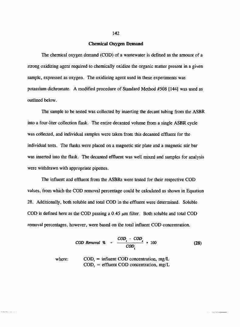
142
Chemical Oxygen Demand
The chemical oxygen demand (COD) of a wastewater is defined as the amount of a
strong oxidizing agent required to chemically oxidize the organic matter present in a given
sample, expressed as oxygen. The oxidizing agent used in these experiments was
potassium dichromate. A modified procedure of Standard Method ^508 [144] was used as
outlined below.
The sample to be tested was collected by inserting the decant tubing from the ASBR
into a four-liter collection flask. The entire decanted volume from a single ASBR cycle
was collected, and individual samples were taken from this decanted effluent for the
individual tests. The flasks were placed on a magnetic stir plate and a magnetic stir bar
was inserted into the flask. The decanted effluent was well mixed and samples for analysis
were withdrawn with appropriate pipettes.
The influent and effluent from the ASBRs were tested for their respective COD
values, from which the COD removal percentage could be calculated as shown in Equation
28. Additionally, both soluble and total COD in the effluent were determined. Soluble
COD is defined here as the COD passing a 0.45 /xm filter. Both soluble and total COD
removal percentages, however, were based on the total influent COD concentration.
COD - COD COD Removal % = * 100 (28)
COD^ ^ '
where; CODj = influent COD concentration, mg/L CODe = effluent COD concentration, mg/L

143
The difference between soluble COD and total COD removal percentages is generally a
measure of the COD of the solids in the effluent.
The COD test was conducted as follows. Effluent and influent samples were
collected from the ASBRs. The samples were mixed well on a magnetic stir plate, and the
appropriate volume of each sample was withdrawn and placed into separate 100-mL
volumetric flasks. These flasks were filled to the lOO-mL mark with deionized and
distilled water. Approximately 30 mL of the diluted effluent samples were then vacuum
filtered through 0.45 fim glass fiber filters (Fisherbrand G4, Fisher Scientific, Pittsburgh,
PA). The filtrate was used in determination of the soluble COD concentration of the
effluent. Five mL of each sample was then withdrawn and placed in a 30-mL screw-top
test tube. Three mL of 0.1 M K2Cr207 were then dispensed into the test tubes, followed
by 7 mL of concentrated sulfuric acid. Table 24 lists the chemical composition of the
various reagents used in the COD test. The test tubes were then capped with phenolic caps
(Corning, Inc., Corning, NY) and placed in a 150°C oven for two hours. At a minimum,
all samples were tested in duplicate. Additionally, four 5-mL samples consisting of
distilled and deionized water were also tested in the manner previously outlined. Two of
these were placed in the oven with the other samples (these were the blanks), and two were
set aside and not placed in the oven (these were the standards).
After heating in the oven, the COD samples were removed and allowed to cool to
room temperature. After cooling, two drops of a ferroin indicator (Table 24) were put
into each sample. The samples were then titrated with 0.1 N ferrous ammonium sulfate

144
Table 24. Reagents used in the COD test. Reagent Solution
Component Name Concentration
COD Acid H2SO4 (conc.) 36.0 N Ag2S04 10.0 g/L
Oxidizing Solution KjCrzOv 4.913 g/L HgS04 33.33 g/L H2SO4 (conc.) 167.0 mL/L H2O 833.0 mL/L
Ferrous Ammonium Fe(NH4)2(S04)2- 6H2O 39.2 g/L Sulfate H2SO4 (conc.) 20.0 mL/L
H2O 980.0 mL/L
Ferroin indicator 1,10-phenanthroline 14.85 g/L FeS04- 7H2O 6.95 g/L H2O 1.0 L/L
(FAS) to the ferroin endpoint. The standards were used to determine the precise normality
of the FAS solution. The blanks provided a measure of the COD of the dilution water.
The COD of a given sample was then calculated as shown in Equation 29.
^ (a - fc)*(jV)*(Df) *(8.000)
c
where, COD = chemical oxygen demand of the sample, mg/L a = volume FAS used for blank, mL b = volume FAS used for sample, mL c = volume of sample, mL
N = normality of FAS solution, equivalents/L DF = dilution factor of the sample
8,000 = equivalent weight of oxygen, mg/equivalent
(29)

145
The variable "c" in Equation 29 was in all cases 5 mL. Since the maximum COD
measurable by this method is 480 mg COD/L for 5-mL samples, the samples normally
required dilution so that the diluted sample had a COD less than 480 mg/L. "DF" in
Equation 29 is the diluted sample volume divided by the undiluted sample volume. For
example, if a sample was diluted by pipetting 20 mL of the sample into a 100-mL
volumetric flask and filling the flask to the 100-mL mark, the dilution factor is 100 mL
divided by 20 mL, or DF = 5. The normality of the FAS solution (N) is calculated using
the standards. The dichromate solution is 0.1 normal. The FAS solution is also made to
be 0.1 N, but this solution photo-degrades over time so that the active normality of the
FAS solution is somewhat less than 0.1, as given in Equation 30.
N = ^ * 0.1 (30)
where, N = acfiaal normality of FAS, equivalents/L (< 0.1) d = volume of FAS used for standards, mL (> 3.0)
3.0 = theoretical volume of FAS required for standards if FAS was exactly 0.1 N, mL
0.1 = theoretical normality of FAS solution, equivalents/L
Volatile Fatty Acids
Volatile fatty acids (VFAs) are classified as water-soluble fatty acids (up to six
carbon atoms) that can be distilled at atmospheric pressure. They are removed from
aqueous solution by distillation despite their high boiling points due to their high vapor
tensions.

146
The VFA concentration of an anaerobic wastewater is a measure of the balance that
exists among the acidogenic, acetogenic, and methanogenic bacterial populations. VP As
arise from the oxidation of sugars, alcohols, lipids, and long-chain fatty acids by the
acidogenic and acetogenic bacteria. Under proper anaerobic digestion, the acetogenic
bacteria convert the VFAs to acetic acid, and the methanogens convert acetic acid to
methane and carbon dioxide. As such, high VFA concentrations signal an upset system in
which the methanogenic bacteria are not keeping pace with the acidogenic and acetogenic
bacteria.
The VFA test was conducted simultaneously with the COD test. Samples for VFA
and COD determinations were taken from the same container. The method employed was
Standard Method #504C [144]. One-hundred mL of the effluent sample was placed in a
500-mL distillation flask, together with 100-mL of distilled water, 5-mL of concentrated
H2SO4, and several glass beads. The flask was placed on a hot plate and connected with an
adapter mbe to a condenser. The samples were then distilled at a rate of approximately 5
mL/minute, and 150 mL of the distillate were collected. The distillate was titrated to the
phenolphthalein endpoint with 0.1 N NaOH, and the VFA concentration in the original
sample was calculated as shown in Equation 31.
_ (a)*(AO*(60,000) «>)*(0.7)
(31)

147
where, VFA = concentration of volatile acids, mg/L as acetic acid a = volume of NaOH used, mL b = volume of sample, 100 mL N = normality of NaOH solution, equivalents/L
60,000 = equivalent weight of acetic acid, mg/equivalent 0.7 = empirical constant
The factor 0.7 is an empirical constant which comes from the assumption that 70% of the
volatile acids will be found in the distillate. The actual value of this constant has been
found to vary between 68 and 85 %, depending on the nature of the acids and the rate of
distillation. Care was taken to be consistent when distilling the VFA samples. The value
of 70% was used in all VFA calculations.
Effluent Suspended Solids
The effluent samples taken for COD and VFA determination were also analyzed for
total suspended solids (TSS) and volatile suspended solids (VSS) using a procedure similar
to 208 D and E of Standard Methods [144]. Since the ASBR system has internal
clarification, the level of TSS is a measure of how well the solids in the ASBR are settling.
A day before the test, the required number of filter papers (Fisherbrand G6,Fisher
Scientific, Pittsburgh, PA) were folded in fourths and placed in aluminum weighing dishes.
These were ignited at 550±10°C for 20 minutes and then cooled to room temperature in a
desiccator for not less than two hours. The filters and dishes were then weighed to the
nearest 0.1 mg on a Mettler model AM 50 digital scale (Mettler Instumentation
Corporation, Hightstown, NJ) and returned to the desiccator until needed. Just before the

148
solids test was conducted, the filter paper and dishes were removed from the desiccator.
The filter apparatus, consisting of a vacuum pump, a 500-mL suction flask, a 4-in
porcelain Buchner funnel, and the necessary connecting hoses, was set up. The filter paper
was removed from the aluminum weighing dish and placed in the Buchner funnel.
The samples to be tested were placed on a magnetic mixer and a specific volume
was withdrawn from the sample with an appropriate pipet. The volume of the sample was
dependent on the approximate solids content of the sample, but was always between 10 and
30 mL. The withdrawn (and a duplicate) sample was pipetted through the filter, and were
then vacuum-filtered until no free water was left on the filter paper. The filter paper was
returned to the weighing dish and these were then transferred to an oven and dried at
103 ± PC for not less than one hour. After drying, the samples were placed in a desiccator
until cooled to room temperature and then weighed. The effluent TSS concentration could
then be determined with Equation 32.
Effluent TSS = *(10®) (32)
where, TSS = concentration of suspended solids, mg/L A = mass of dish + filter after drying at 103°C, grams B = initial mass of dish + filter (before filtering), grams V = volume of sample filtered, mL
10^ = conversion from g/mL to mg/L
The effluent VSS were determined by igniting the dried samples from above at 550±10°C
for 20 minutes. These samples were then cooled to room temperature and weighed again.

149
The residue remaining on the filter after ignition represents the fixed, or nonvolatile
fraction, since the volatile portion has been destroyed. Equation 33 was used to determine
the effluent VSS.
Effluent VSS = ^*(10®) (33)
where, VSS = concentration of suspended solids, mg/L A = mass of dish + filter after drying at 103°C, grams C = mass of dish + filter after igniting at 550°C, grams V = volume of sample filtered, mL
10® = conversion from g/mL to mg/L
Mixed Liquor Suspended Solids
The mixed liquor suspended solids (MLSS) and mixed liquor volatile suspended
solids (MLVSS) are a measure of the suspended solids in an operating ASBR. The MLSS
is the concentration of all solids with an effective diameter greater than 0.45 fim, whereas
the MLVSS measures only the volatile fraction greater than 0.45 fim. The MLVSS is a
better measure of viable biomass, although neither MLSS nor MLVSS is a true measure of
the amount of active microbes present. MLVSS is typically used to approximate the
organic solids present in a reactor. The different between volatile and organic matter is
generally due to the volatilization of some inorganic compounds, most notably inorganic
carbonates. That is, some inorganic carbonates are volatilized in the test and do not show
up as fixed solids but rather as volatile solids. Therefore, equating organic residue with

150
volatile residue would be in error. Despite the differences in the two parameters, volatile
solids were used to approximate the viable fraction because of the relative ease of the
MLVSS test as compared to the total organic carbon test.
The samples used in the MLSS test were taken directly from the ASBRs during
mixing. A side port was used to release approximately 20 mL of the ASBR contents into a
beaker, and this volume was discarded. This was done to empty the side port of its
contents, since the solids present in these ports are not representative of those present in
the ASBR active volume. Another sample (30 to 40 mL) was then withdrawn from the
same port and used for the MLSS test.
Filter papers were prepared exactly as in the effluent suspended solids test. Five
mL of the MLSS samples were then filtered (in duplicate) and the excess water was
removed with the vacuum pump. The samples were then dried in a 103 ± PC for not less
than one hour. After drying, the samples were placed in a desiccator until cooled to room
temperature and weighed. The MLSS concentration could then be determined with
Equation 32, except that the effluent TSS term was replaced with MLSS.
MLVSS concentrations were determined by igniting the MLSS samples at 550°C for
20 minutes. After ignition of the samples, the filter papers were cooled and weighed. The
MLVSS concentration was then calculated with Equation 33, except that the effluent VSS
term was replaced with MLVSS.

151
Hydrogen Ion Concentration
One of the most important operating parameters of an anaerobic system is pH.
Although acidogens and acetogens are able to survive over a fairly wide range of pH,
methanogens can generally grow only within a pH range of approximately 6.5 to 7.8. The
optimum pH is near 7. It was, therefore, necessary to monitor the pH daily for any
significant deviation from near-neutral pH conditions.
Samples of the effluent from the ASBRs were collected in beakers for pH
determination. The pH was measured using a Cole-Parmer model 05669-20 pH meter
(Cole-Parmer Company, Chicago, IL) which was calibrated before each use using standard
pH solutions of 4.00 and 7.00. or 7.00 and 10.00, depending on the pH of the ASBR
effluent.
Alkalinity
The alkalinity of a water or wastewater is its quantitative capacity to neutralize
strong acid to a designated pH. Alkalinity in anaerobic systems is an important parameter
in that volatile acids produced by acidogenic and acetogenic bacteria tend to lower reactor
pH. Sufficient alkalinity is necessary to maintain the pH of the system at or near 7.
In many wastewaters, alkalinity is a function of the carbonate, bicarbonate, and
hydroxide content. In waters containing significant phosphates, silicates, and borates, the
total alkalinity is also a function of these species. At typical pH values found in anaerobic
systems (pH = 6.7 to 7.5), the hydroxide and carbonate concentrations are negligible as

152
compared to the bicarbonate concentration. Therefore, total alkalinity is essentially equal
to bicarbonate alkalinity (plus borate, phosphate, and silicate alkalinity, if applicable).
For the two substrates used in these experiments (sucrose and beef
extract+glucose), alkalinity was added to the feed solutions in the form of NaHCOa.
Additionally, alkalinity was produced in the reactors in the form of ammonium bicarbonate
(NH4HCO3). The sucrose substrate contained no nitrogen, and, therefore, all of the
ammonia for these experiments was derived from addition of NH3 to the feed solutions.
The beef extract substrate, however, contained a significant amount of protein, the
degradation of which resulted in additional ammonia generation within the ASBRs. The
bicarbonate species were derived from two separate sources. First, bicarbonate was added
directly to the reactor feed solutions, as mentioned earlier. Second, degradation of the
substrates resulted in COj production. CO2 is in equilibrium with bicarbonate at the pH
levels present in these systems. Therefore, CO2 production leads to bicarbonate
production. Equations 34 and 35 illustrate the production of alkalinity from ammonia,
carbon dioxide, and water.
AW3 + CO2 + H^O NHflCO^ ^ NH^ + HCO^
HCO; + H* ^ HjCOj ^ CO^ + Hp
(34)
(35)

153
Additionally, HCO3" and NH4^ are in equilibrium with CO3" and NHj,
respectively. However, at the pH levels in these experiments, the latter two species
represent an insignificant contribution to the buffering capacity of the system.
Standard method 403 [144] was used to determine the total alkalinity of the ASBR
effluents. Potentiometric titration to pH 4.5 was performed with 0.1 N sulfuric acid
throughout all experiments. The procedure was as follows. A 25-mL sample was
collected in a beaker from an ASBR during the decant phase of a given cycle. The sample
was quickly placed on a magnetic stir plate and a magnet stir bar was placed in the sample
beaker. A calibrated pH electrode was inserted into the sample and the sample was mixed
thoroughly. The sample was then titrated with 0.1 N sulfuric acid to pH 4.5. The total
alkalinity of the sample was then calculated using Equation 36.
Alk - (36)
where, Alk = total alkalinity, mg/L as CaCOj A = volume of standard acid used, mL N = normality of standard acid, equivalents/L V = volume of effluent sample titrated, mL
50,000 = equivalent weight of CaCOs, mg/equivalent
Ammonia Concentration
The ammonia concentration in the ASBR is important for two reasons. A very low
ammonia concentration may be indicative of a nitrogen-limited system, which would result
in poor substrate removal efficiencies due to lack of bacterial growth. Conversely, a high

154
ammonia concentration could lead to inhibition of the microorganisms due to ammonia
toxicity. Since ammonia was added to the substrate feed solutions in sufficient
concentration to ensure the nitrogen was not limiting, the main reason for determining
ammonia concentrations was to test for possible ammonia toxicity.
The literature generally implicates an inhibitory effect on methanogenesis at total
ammonia (NHj + NH4^) concentrations of approximately 1,500 mg/L, as N. A more
detailed description of ammonia toxicity is presented in the Literature Review section.
Since the sucrose substrate did not contain nitrogen, almost all of the ammonia present in
the system was due to the addition of NH4OH to the feed solutions. Additional ammonia
may be produced through cell death (followed by proteolysis), however, cell uptake of
ammonia during biosynthesis is greater than the amount of ammonia produced by cell
death in a system operating efficiently (cell growth ^ cell death unless the system is
inhibited or failing). Therefore, the concentration of ammonia in the ASBR systems is
generally not greater than the amount of ammonia added to the feed solutions. In other
words, the maximum ammonia concentration in the ASBRs fed the sucrose substrate could
be calculated without actually testing for ammonia.
In the systems fed the beef extract + glucose solutions, however, degradation of
the protein fraction of the beef extract led to additional ammonia production, the extent of
which was dependent on the efficiency of protein breakdown. It was, therefore, necessary
to measure the ammonia concentration of the ASBR effluent to ensure that ammonia
inhibition did not occur.

155
An Orion ammonia probe (model 95-12, Orion Research Inc., Boston, MA) was
used with an Altex model 4500 combination pH meter and millivolt potentiometer
(Beckman Scientific Instruments, Irvine, CA) to determine total ammonia concentrations.
The ammonia probe was calibrated with ammonium chloride solutions of 10, 100, 1,000,
and 5,000 mg/L, as NH3. A standard curve was calculated for these standard solutions.
Twenty mL samples were obtained from the ASBR effluents. The ammonia probe was
then inserted into the sample (while mixing) and 2 mL of 6 N NaOH was added to the
sample to increase the pH to above 11, which ensured that all of the ammonia would be in
the unionized form (the ammonia probe measures NH3, not NH4^). The millivolt reading
could then be compared to the standard curve to calculate the total ammonia concentration
of the ASBR effluent.
Biogas Production and Composition
Methane and carbon dioxide (collectively termed here as biogas) are produced by
the anaerobic consortia in the ASBR and other anaerobic reactors. The acidogens and
acetogens oxidize higher organic molecules in a waste to long and short chain fatty acids,
such as acetate, propionate, butyrate, and others. Little overall reduction in COD of the
materials occurs in these steps since the degradation products are not liberated from the
system. Stated differently, the COD of the degradation products in a given waste is
approximately equivalent to the COD of the starting materials in the waste. During
methanogenesis, however, stabilization of the waste occurs due to the liberation of

156
methane. Therefore, measurement of methane production is a useful tool for determining
the degree of COD stabilization of a waste.
The COD-equivalent of the methane produced from anaerobic degradation of an
organic susbstrate can be calculated by Equation 37.
CH^ + 20^ - COj + 2Hfi (37)
The COD-equivalent of methane is, therefore, 2 moles of COD (oxygen) per mole of
methane produced. Equivalently, the COD-equivalent is 0.35 L CH4/g COD removed, or
5.61 ft^ CH4/lb COD removed (all values are at standard temperature and pressure, 0°C
and 1 atm.). Analysis of the composition of biogas produced from a reactor can then be
used to determine the volume of methane produced, which enables a calculation of COD
stabilized in the reactor. An example of this procedure is given below.
Given: COD feed rate = 1 g COD/L of reactor/day
reactor volume 5 L
biogas production 2.5 L/day (STP)
CH4 % of biogas 65%
Solution: CH4 production = (0.65)(2.5 L/day) = 1.625 L/day (STP)
COD stabilized = 1.625 (L/day)/(0.35 L/g COD) = 4.64 g/day
COD in feed = (5 L)(l g COD/L/day) = 5 g/day
% COD reduction = (4.64 g/day)(100)/(5 g/day) = 92.86%

157
As outlined in the Setup section of this document, the daily biogas production was
measured with wet-test gas meters. The meter reading was taken at ambient atmospheric
pressure and SSiO.S^C, both of which were recorded daily. The daily biogas volumes
were then expressed as standard biogas production at 1 atm and 0°C. The biogas
composition was analyzed using gas chromatography (GC). The GC system included a
Model 69-350 Thermal Conductivity Gas Chromatograph (GOW-MAC Instrument
Company, Bridgewater, NJ), equipped with a 6-ft. long by 1/8-in. in diameter GC colunm
with Porapak-Q 80/100 mesh column packing. The operating conditions and parameters
for the GC analysis are listed in Table 25.
Samples were collected using a l-mL syringe (Hamilton Company, Reno, NV)
equipped with 2-in-long Metal Hub Needles (Alltech Associates, Inc., Deerfield, IL).
Nine-tenths of a mL of biogas was withdrawn from the gas sampling ports (earlier
described) and the gas was then injected into the injection port of the gas chromatograph.
The data from the gas analyses were collected and analyzed using the Baseline 810
Chromatography Workstation software package (Waters Dynamic Solutions, Division of
Millipore, Venmra, CA). The output from the analyses listed the percentages of methane,
carbon dioxide, and nitrogen in the biogas. The nitrogen percentage in the biogas was
actually a measure of the amount of air in the system. Theoretically, there should be no
air in the system, since oxygen is toxic to anaerobic organisms. However, a small amount
of air will enter the reactor due to the solubility of these gases in the feed substrate. In a
well-operated system, oxygen entering the reactor through the influent will rapidly be

158
scavenged by facultative organisms and other oxygen-demanding substances. Therefore,
the amount of nitrogen in the biogas was reflective of the air-tightness of the system.
Zero, or very low, nitrogen indicated that the system was air tight, and significant nitrogen
in the biogas suggested that there was a gas leak in the ASBR or gas handling equipment.
Table 25. Gas chromatography analysis setup. Parameter Value
Column temperature, °C ambient
Injector port temperature, "C 100.0
Detector temperature, °C 150.0
Outlet temperature, "C 70.0
Biogas sample volume, mL 0.9
Column packing
length, ft 6.0
diameter, in 0.38
Carrier gas helium
Carrier gas flow rate, mL/min 60.0
Standard gas
methane, % 70.0
carbon dioxide, % 25.0
nitrogen, % 5.0

159
Automated Image Analysis
Automated image analysis (AIA) was utilized to monitor the changes in biomass
particle morphology and size in the ASBRs. Each ASBR was initially seeded with
flocculent anaerobic digester sludge. Over time, the biomass particulates (which may
or may not be biological in nature) tend to mature into large pellets, or granules. Whereas
the average particle size at the beginning of each study was approximately 30 fim, over
time the average particle size grew to several hundred microns, depending on the degree of
granulation achieved in each ASBR. By monitoring the growth of the particle size, the
physical transformation of flocculent biomass to granular biomass could be correlated with
the operational state of the ASBR over the same time frame.
The AIA system was located at the Materials Testing Laboratory within the
Department of Civil and Construction Engineering at Iowa State University. The AIA
system consisted of a light microscope (model SZH, Olympus, Japan) with a video adaptor
(Series 68, Dage-MTI, Michigan City, IN) connected to a video monitor (Sony Trinitron,
Japan). The monitor was connected to a computer (model CIT-101 video terminal, C. Itoh
Electronic, Inc., Los Angeles, CA) which analyzed the video images as presented below.
The software used for analyses was OASYS 3 (LeMont Scientific, State College, PA).
The biomass sample to be analyzed was taken from the respective ASBR in a
manner identical to the procedure for MLSS analysis. The sample was mixed on a
magnetic stir plate and a broken tip pipette was used to transfer approximately 2 mL of the

160
sample to a modified well slide. The slide was then placed on the microscope platform and
was ready for analysis.
The first step of analysis was to focus the microscope on the biomass in a way such
that the majority of the biomass on the slide was in focus. Because the biomass was
actually contained over the entire depth of the biomass slide, it was not possible to focus
the entire contents of the sample at any given time. After focusing, the software was
operated as follows. The unage of the biomass was captured as a graphics file. The
software then "colored" the biomass red, leaving the background liquid white. The
software then calculated the area of each particle of biomass and calculated an equivalent
diameter assuming the particles were spherical. The output from the software included
histograms of the size distributions and total mass distribution, as well as average
characteristics of the entire sample. Several analyses were made for each sample, and the
cumulative results were then printed out for further analysis.
Specific Methanogenic Activity
Activity tests were conducted on the biomass from selected ASBRs to determine the
differences between the specific substrate removal rates of fiocculent and granular biomass.
In this context, specific methanogenic activity (SMA) is defined as the rate of methane
production per unit of biomass, and is defined for the entire bacterial consortium (not only
methanogenic organisms). Previous research [87] in the environmental engineering
laboratory at ISU indicated that granular biomass has a distinctly higher SMA than that of

161
flocculent biomass under identical conditions. It was also noted in the first few
experiments of this research that when the biomass began to granulate in any given
experiment, the biogas production rate (COD removal rate) increased significantly over a
short period, and that this increase was proportionately greater than the increase in biomass
concentration over the same time period. It was then decided that SMA tests should be
conducted to quantify this observation.
The SMA tests were originally designed to be conducted in an anaerobic
respirometer, but because of difficulties with the unit, it was decided to do the SMA tests
in sim (using the entire ASBR). This change lead to several difficulties. The
environmental conditions were more difficult to maintain and monitor in the ASBR as
compared to a small respirometer bottle. Also, it was more difficult to maintain uniform
mixing conditions in the ASBR than it would have been in a small bottle. The ASBRs had
to be continuously mixed at a high rate to maintain complete mix conditions. Also, the
substrate concentrations added to the ASBRs were very high compared to the concentration
that the microbes had been accustomed to seeing. It was observed that some of the
granules in the SMA tests were damaged by shear or high rate of gas production.
Therefore, because of the nature of the SMA test in the ASBR, it was not conducted during
all of the experiments. Nevertheless, the ASBR units provided a comparative measure of
the SMA characteristics of the various biomasses tested.
The SMA test was conducted as follows; The ASBRs to be tested were not fed for
a period of 12 to 24 hrs before the SMA test in order to decrease the background substrate
162
concentration to its minimum level. The MLSS and MLVSS concentrations of the ASBRs
were determined the day before the SMA test, since the amount of substrate added per unit
mass of MLVSS was kept at a constant value for these tests. Just before the substrate was
added to the reactors, a concentrated solution of sodium bicarbonate and appropriate
nutrients and trace minerals were injected into the ASBR with a syringe. The amount of
these compounds added was in proportion to the amount of COD added. These
proportions were identical to those used to prepare the substrate feed solutions (described
earlier). The substrate was then injected into the ASBR with a syringe, and the gas meter
reading was recorded. Over the next 4 to 10 hours, the gas meter readings were recorded
over time. Every 15 to 30 minutes, GC analyses of the biogas were conducted to
determine the methane percentage of the total biogas. The pH in the ASBRs was
maintained between 6.9 and 7.1 by syringe injection of HCl or NaOH, which ever was
appropriate.
The cumulative methane production per unit mass of MLVSS over time was then
plotted, yielding a linearly increasing portion over the first time period, which then level
off to a maximum cumulative methane production for the amount of substrate added. The
linear portion of the curve was indicative of the maximum SMA of the biomass.
Two different substrates were used in the SMA tests to determine whether granule
morphology and consortia arrangement was the cause of the higher SMA for granules as
compared to flocculent biomass. Sucrose, which requires the interaction of the entire
bacterial consortia for conversion to methane, and acetate, which only requires the

163
methanogenic bacteria for conversion to methane, were utilized. It was predicted that the
granular biomass would yield a higher SMA for sucrose, as compared to the flocculent
biomass, but that the SMA for acetate would be similar. Discussion of this phenomenon
can be found in the results and discussion portion of this document.
Scanning and Transmission Electron Microscopy
Scanning and transmission electron microscopy (SEM and TEM, respectively)
analyses were also performed on the biomass from the ASBRs to observe the morphology
and general nature of the granules developed in the experiments. Direct observation of the
bacterial consortium within each granule allowed a qualitative estimation of similarities and
differences among the granules developed in each of the experiments. In other words, if
one experiment yielded a granule mainly consisting of cocci, while the granules from
another experiment were composed of mainly rods, one plausible explanation for this is
that the experimental enhancement method utilized in those experiments physically selected
for those types of bacteria.
It was also desired to observe the homogeneous or heterogeneous distribution of the
bacterial consortium of the granules. That is, the use of electron microscopy could
elucidate whether the granule consisted of layers, with each layer consisting of a different
bacterial group, or if the granules were homogenous throughout, with all groups of
bacteria present in each part of the granule.

164
The SEM and TEM analyses were conducted at the Bessey Microscopy Facility,
located at Iowa State University. Selected samples were taken to this facility, and all
preparatory work and analyses were performed by the Bessey staff. The SEM used was a
JEOL model JSM-35 opearted at 15 kV. The samples were prepared with a Polaron
sputter coater, using a palladium/platinum mixture.
Elemental Analysis of Blomass
Several reports in the literature have cited significant amounts of specific inorganic
compounds or elements in granules. Others have noted that the elemental distribution of
granules is very similar to that of fiocculent biomass. It was decided to have the granules
developed in these experiments examined for the constitutive composition of a range of
elements (Table 26). An understanding of the elemental nature of granules,
although not a significant contribution of this research, could lead to fiiture research
centered on the chemical enhancement of granulation.
The elemental and chemical analyses of the granules was conducted at the
Analytical Services Laboratory (ASL) located within the Department of Civil and
Construction Engineering at Iowa State University. All analyses were conducted by ASL
staff. The samples to be analyzed were taken from the ASBRs after the respective
experiments had been shut down. The samples were prepared for analysis using the
methods shown in Table 26.

165
Table 26. Elemental analysis of granules. Element/Compound Method of Analysis Carbon, organic Total organic carbon^
Nitrogen, total kjeldahl Auto-analyzer''
Phosphorous Auto-analyzer*^
Potassium Atomic absorption*"
Sodium Atomic absorption''
Calcium Atomic absorption''
Magnesium Atomic absorption''
Iron Atomic absorption''
Zinc Atomic absorption''
Nickel Atomic absorption''
Cobalt Atomic absorption''
Manganese Atomic absorption''
" Dohrman Total Organic Carbon Analyzer (Rosemount Analytical Division, Santa Clara, CA). '' Technicon Autoanalyzer II (Technicon Instruments Corporation, Tarrytown, NY). ' Technicon Autoanalyzer 11 (Technicon Instruments Corporation, Tarrytown, NY). '' Smith Hieftje 12, Model 857 (Instrumentation Laboratory, Inc., Lexington, MA).

166
RESULTS AND DISCUSSION
The following pages present a summary of the data collected over the course of this
research. The data are presented individually for each of the different granulation-
enhancement experiments. That is, all of the data for the PAC-enhancement is presented
in one section, all of the data for the cationic polymer-enhancement is presented in another
section, an so on. After the enhancement data has been presented, other data will be
presented regarding the SMA tests, elemental analyses, and SEM analyses of the various
biomasses produced during the experiments. Data tables, if not presented within the text
of this section, are located in the appendices located at the end of this document. The
Table of Contents and List of Tables details the organization of the document.
It is important to realize that these were not equilibrium studies. The goal of each
study was to achieve granulation and system start-up in a short period of time. Therefore,
the systems were pushed to their limits during their start-up period, and the line between a
slightly-stressed and a heavily-stressed reactor was sometimes crossed. The goal was to
slightly stress the systems in order to achieve high OLRs and short HRTs. In theory, these
conditions should present the best physical conditions for granulation. The short HRT
washes out the poor-settling biomass, and the high OLR creates conditions for high
biomass production rates and high MLSS levels.
As previously stated, the data presented in this section reflect the stressed, non-
equilibrium conditions in the reactors. Few of the curves consist of tightly grouped or
smooth data points. Several of the graphs show sudden changes in the respective

167
parameters that are presented. The data presented here have not been "smoothed" by
eliminating wild points, since the wild points were normally the result of an actual
condition rather than a poorly-executed analysis. Instead, these wild points will be
explained as to their cause and significance. The recovery of the systems from the highly-
stressed conditions is also discussed, including the overall effect on granulation and start
up.
Sucrose Experiments
The majority of the granulation/start-up experiments were conducted using sucrose
as the sole carbon source. Sucrose was selected for several reasons: (1) Sucrose is
relatively easy to work with and is highly soluble in water. COD concentrations could be
maintained at any desired level, resulting in a flexible COD loading rate. (2) The solutions
of sucrose in water did not separate or precipitate over time. Additionally, the sucrose
solutions could be kept in the constant temperature room at 35°C for two days before
noticeable degradation occurred. (3) Sucrose conversion to methane requires anaerobic
bacteria from all of the previously-discussed groups. And (4) sucrose and related sugars
are typical constituents of several industrial wastewaters.
Control Study
It was necessary to establish a baseline control for granulation and start-up using
the sucrose substrate. As previously stated, the only other granule-producing study

168
conducted with the ASBR used a non-fat dry milk substrate and required over 200 days for
significant granulation to occur. The control study in these experiments was conducted
exactly as the other experiments, with the exception that no granulation enhancement was
practiced.
Operational Performance
The control ASBR was seeded with an MLSS concentration of approximately
20,000 mg/L (MLVSS approximately 12,000 mg/L). The HRT and COD loading rate
were initially 2 days and 1 g/L/day, respectively. After approximately one week, the COD
load was increased to 2 g/L/day at an HRT of 2 days. These conditions were maintained
in the ASBR for a period of approximately 1 month due to the poor COD removal
efficiency and methane production (Figures 18 and 19). It is noted here that in Figure 19
and subsequent standard methane production curves, the relative height of the methane
curve to the COD load curve is approximately the COD removal efficiency of the system
based on methane production. This results from the graphical method chosen to present
these data. The scale of the primary Y-axis (methane production) has been set at one-third
of the scale of the secondary Y-axis (COD-load). The theoretical methane yield from 1
gram of COD removed is 0.35 L, which is very close to one-third. In fact, taking into
consideration biosynthesis, the value of one-third is a more realistic methane yield constant
than 0.35.

169
100
90
80
70
1 50 V
oe Q 40 O u
30
20
10
0
Soluble Removal
Removal
20
18
16
14 _
•I"
1 0 #
8
6
4
2
0
a o
20 40 60 80 100 120 140 160 180 200 Time Since Start-Up (days)
Figure 18. COD removal for the sucrose control study.
5.0
4.5 relative height of the methane curve to the COD load curve = approximate COD removal based on methane
COD Load
Methane
25 50 75 100 125 150 Time Since Start-Up (days)
Figure 19. Methane production for the sucrose control study.

170
After 35 days of operation, the HRT was decreased to 36 hrs and 12 days later to
24 hrs, where it remained for the remainder of the experiment. After more than 70 days
of operation, the soluble COD (SCOD) removal efficiency increased to over 70%, at which
time the COD load was increased to 2.5 g/L/day. On day 100, the COD load was further
increased to 3.5 g/L/day, and shortly thereafter to 5 g/L/day (day 122). After this time,
the COD load was increased step-wise to a high of 12 g/L/day on day 145, with greater
than 85% SCOD removal at most loading rates.
After a period of 2 weeks at 12 g COD/L/day, the reactor began to fail. The COD
removal decreased (Figures 18 and 19) and the volatile acids concentration increased
(Figure 20). The pH dropped slightly, but remained within acceptable limits (Figure 21).
On day 162, the COD loading rate was decreased to 6 g/L/day and shortly thereafter the
reactor was shut down.
Solids and Granulation
The MLSS levels in the control ASBR continued to decrease until reaching a
minimum of 4,000 mg/L on day 84. After this time, the MLSS concentration continually
increased to a maximum of almost 18,000 mg/L on day 159, at which time the COD load
was 12 g/L/day. Simultaneous with the decreased COD removal observed at 12 g
COD/L/day, the MLSS level abruptly decreased to below 14,000 mg/L. It was observed
that the excessive biogas production resulted in very mrbulent conditions during the settle

171
3,000
2,700
2,400
S 2,100 14
(J 1,800 es §. 1,500
Load Acids I.. u 1,200
900
300
0 20 40 60 80 100 120 140 160 180 200 Time Since Start-Up (days)
Figure 20. Volatile acids data for the sucrose control study.
2,000 rS.O
1,800 4) 1 1,600 A S 1,400
7.8 I AUcaUnity I
7.6
7.4
1,200 7.2
1,000 7.0
800 6.8 CL
6.6
6.4 400
200 6.2
i6.0
0 20 40 60 80 100 120 140 160 180 200 Time Since Start-Up (days)
Figure 21. Alkalinity and pH data for the sucrose control study.

172
and decant phases. Therefore, the solids did not settle as well and were carried out in the
effluent (Figure 22).
The sludge age of the system was generally in excess of 10 days for the first 100
days of operation. However, over the same period in which the COD removal efficiency
improved drastically and the MLSS levels increased, the sludge age was consistently below
10 days with an average of approximately 7.5 days. This low SRT did not appear to be
detrimental to the overall process. In fact, the ASBR performed significantly better over
the time period during which the SRT was below 10 days (Figure 22).
Figure 23 presents the granulation data for the control reactor. Again,
approximately at day 100 changes begin to occur. The biomass was decidedly floccuient
over the first 4 months of operation. However, the AIA on day 120 revealed a slight
increase in the average biomass particle size over previous tests, although visually the
biomass still appeared to be almost completely non-granular. Approximately two weeks
later, significant granulation was observed. The granulation of the biomass correlates well
with the observed COD removal performance over the same time period. That is, as
the biomass granulated, the COD removal efficiencies increased significantly, even as the
COD load approached 12 g/L/day.
Two notes are relevant here. The first is that the SRT of the system (and of
systems presented in the following paragraphs) was below the theoretical minimum for
anaerobic systems. As stated earlier, the minimum SRT of an anaerobic system is
normally around 10 days. Below this SRT, methanogens are washed out of the reactor at a

173
20,000 100
18,000
MLSS
10,000
8,000
6,000
4,000 sludge age
2,000
0 20 40 60 80 100 120 140 160 180 Time Since Start-Up (days)
Figure 22. MLSS and SRT for the sucrose control study.
2,250
2,000
E 3 U v
1,750 geometric average
1,500 a>
s 1,250
I 1,000
iS 750
> 500
arithmetic average
250
"'1 i
20 0 40 60 80 100 120 140 160 180 200 Time Since Start-Up (days)
Figure 23. Average particle size data for the sucrose control study.

174
rate faster than they can reproduce. One explanation is that as granulation progresses, the
biomass becomes segregated in the reactor, resulting in non-complete mix conditions and
an underestimation of the MLSS (and SRT). A second explanation is that the
methanogenic growth rates of granular biomass is higher than that of non-granular
biomass. Under optimum growth conditions in pure culture, the doubling times of most
methanogens is approximately 3 to 7 days. It, therefore, appears that the micro-
environment that exists in a granule may approximate optimum growth conditions,
allowing for faster growth rates than is possible for non-granular biomass (better
thermodynamics).
The second note is a distinction between the average particle size based on the
number of particles (arithmetic) and based on the weight distribution of the particles
(geometric). Based strictly on the diameter of each particle in a given biomass sample, the
average particle diameter of the sample may be quite small. However, in that same sample
the majority of the mass of the sample may be incorporated in granules. The geometric
average particle diameter is a measure of the distribution of the biomass in each range of
particle size, and, therefore, better reflects the average state of granulation.
It is further noted that although the two parameters normally trend together, the absolute
values of the two are quite different. Both the arithmetic and geometric average particle
size are presented throughout this document. However, the geometric average particle size
is considered to be more significant in terms of defining granulation.
175
Powdered Activated Carbon Enhancement Study
Powdered activated carbon (PAC) was used to enhance granulation. It was
theorized that the PAC would act as a site of attachment for bacteria. The PAC adsorbs
substrate molecules and thus should provide an ideal site for bacterial growth and
granulation. This experiment was the longest of all of the experiments in this study. It
was decided to try to achieve the highest possible COD load on the ASBR after granulation
had been observed.
Operational Performance
The PAC-enhanced ASBR was seeded with an MLSS concentration of
approximately 20,000 mg/L (MLVSS approximately 12,000 mg/L) and a PAC
concentration of 2,000 mg/L. After the initial addition of PAC to the ASBR, no ftirther
additions were made. The HRT and COD loading rate were initially 2 days and 1
g/L/day, respectively. After 3 weeks of operation, the COD removal improved enough to
increase the OLR to 2 g COD/L/day (HRT = 2 days). After 45 days of operation, the
COD removal and settling improved and the HRT was reduced to 1 day. The COD load
was further increased to 3 and 4 g/L/day on days 65 and 90, respectively. At
approximately day 105, the COD removal increased significantly, and the COD load was
step-wise increased to 5, 7, 9, 11, and 14 g/L/day over the next 45 days. Over this period
of time, the SCOD removal efficiency of the ASBR was in excess of 95% at all loads, and
the total COD (TCOD) removal efficiency was approximately 70 to 80% (Figures 24 and

176
25). The volatile acids concentration over this same time period was low (Figure 26), and
even at the COD load of 14 g/L/day was below 100 mg/L (as acetic acid). The pH
remained relatively constant between 6.8 and 7.0 (Figure 27).
After approximately 20 days operating at 14 g COD/L/day, a sudden pH drop (pH
= 5.3) caused the failure of the system (Figures 24-27). COD removal was negligible and
the volatile acids increased to 2,600 mg/L. It was not explicitly known what caused the
severe pH drop, but it seems likely that the buffering compounds (sodium bicarbonate and
ammonium hydroxide) may have been left out of the feed solution.
Although complete failure of the methanogens was apparent (zero gas production),
conversion of the sucrose to acids was observed, and, therefore, the entire system was not
dead. The COD load was decreased to 3.5 g/L/day to try to recover the methanogenic
activity. After approximately 3 weeks, the SCOD removal increased to 90%, and the
COD load was step-increased to 12 g/L/day over 50 days. Although the COD removals
were generally in excess of 90% at loads of 9 g COD/L/day and less, the
system began to fail again at 12 g/L/day. Again, the pH of the reactor decreased at this
time (pH = 6.5). The reactor was shut-down shortly after this second pH decrease.
The recovery of the ASBR observed after complete methanogenic shut-down is
significant. It is probable that the granule envirorunent protects the methanogens to some
degree from inhibitory conditions, such as the low pH observed in this study. One theory
is that ion diffusion is limited into the granule. Under normal conditions the granule
matrix provides an efficient route for transfer of metabolic intermediates. Under stressed

177
Soluble Removal
Total Removal
25 50 75 100 125 150 175 200 225 250 275 300 Time Since Start-Up (days)
Figure 24. COD removal for the PAC-enhanced sucrose study.
relative height of the methane curve to the COD load curve = the approximate COD removal based on methane
COD Load
Methane
0 25 50 75 100 125 150 175 200 225 250 275 300 Time Since Start-Up (days)
Figure 25. Methane production for the PAC-enhanced sucrose study.

178
COD Load
0 25 50 75 100 125 150 175 200 225 250 275 300 Time Since Start-Up (days)
Figure 26. Volatile acids data for the PAC-enhanced sucrose study.
3,500
3,250
£ 3,000
I 2,750 g 2,500
a 2,250
I 2,000
I 1,750 ij 1,500
11,250 1,000
^llkalinit^
75 100 125 150 175 200 225 250 275 300 Time Since Start-Up (days)
Figure 27. Alkalinity and pH data for the PAC-enhanced sucrose study.

179
conditions, this same property may limit the amount of inhibitory substance entering the
granule, thereby reducing the adverse effect on the bacterial consortia.
Solids and Granulation
The MLSS levels in the PAC-enhanced ASBR quickly decreased to their minimum
level shortly after start-up (Figure 28). The MLSS concentration decreased from
approximately 21,000 mg/L at day zero to 5,000 mg/L at day 20. The solids stayed at this
level until approximately day 60, at which time they began to increase slowly. At day 90,
the MLSS concentration was approximately 9,000 mg/L, and stayed at this level until
about day 125. Over the next 50 days, the MLSS level increased to more than 26,000
mg/L. Over this same time period, the COD loading rate was increased from 5 to 14
g/L/day. Upon reactor failure at day 165 (presented earlier), the MLSS concentration
decreased to less than 15,000 mg/L over 40 days. Later, the recovery of the system
resulted in an increase in the MLSS level to 27,000 mg/L. The SRT of the system
flucmated around the 10-day mark for the majority of this study (Figure 28). As the
MLSS continued to increase, the effluent solids concentration also increased, resulting in a
relatively constant SRT. Figure 29 presents the granulation data for the PAC-enhanced
ASBR. The first granules were observed at approximately day 90, although at this time
the majority of the biomass was still flocculent. From day 90 to day 120, significant
granulation was observed. By day 130, the geometric average particle diameter was in
excess of 1.5 mm, and just prior to reactor failure the average size was over 2.2 mm. The

180
30,000 100
27,000 90
MLSS 24,000
5 21,000 ec B r 18,000
15,000 •o -S 12,000
S 9,000
6,000
I Sludge Age |
20
3,000
0 25 50 75 100 125 150 175 200 225 250 275 300 Time Since Start-Up (days)
Figure 28. MLSS and SRT for the PAC-enhanced sucrose study.
2,500
2,250
f 2,000 3-U 1,750
1 1>S00 <§ » 1,250
I 1,000
§> 750 s I 500
250
0
0 25 50 75 100 125 150 175 200 225 250 275 300 Time Since Start-Up (days)
geometric average
arithmetic average
Figure 29. Average particle size for the PAC-enhanced sucrose study.

181
failure of the ASBR due to low pH also affected the particle size of the granules.
Significant breakup of the granules was observed, and the average size decreased to
approximately 1 mm. During reactor recovery, the average size again increased to over
1.5 mm.
PAC Effect
Compared to the control reactor, the PAC-enhanced ASBR was observed to
granulate more rapidly. The PAC-enhanced ASBR was approximately one month ahead of
the control ASBR in terms of first detection of granules and overall granulation of the
biomass. The PAC-enhanced ASBR was also able to achieve higher OLRs more quickly
than the control reactor. After 90 days of operation, the control reactor was operating at
2.5 g COD/L/day and removing 60% of the SCOD. After 90 days in the PAC-enhanced
ASBR, however, it was treating 4 g COD/L/day at over 70% SCOD removal. Shortly
thereafter the SCOD removals increased to over 95%. It seems apparent that the effect of
the PAC addition was beneficial to the overall function of the ASBR.
Granular Activated Carbon Enhancement Study
Granular activated carbon (GAC) was also used as an enhancement for granulation
and ASBR start-up. Several studies with the expanded-bed anaerobic reactor (presented
earlier) indicated significant growth attached to GAC. GAC also offers the advantage of

182
better settling properties as compared to PAC. Therefore, biomass attached to GAC has a
better chance of remaining in the reactor as compared to biomass attached to PAC.
Operational Performance
The GAC-enhanced ASBR was initially seeded with 19,000 mg/L of suspended
solids (MLVSS = 11,400 mg/L) and 2,000 mg/L of GAC. The initial HRT and OLR
were set at 2 days and 1 g COD/L/day, respectively. After 2 weeks the COD load was
increased to 2 g/L/day (1-day HRT), and by day 40 the reactor was treating 4 g/L/day at
approximately 70% SCOD removal efficiency (Figures 30 and 31). At approximately day
60 the COD load was increased to 5.5 g/L/day. By day 90, the load was at 9 g/L/day with
over 90% SCOD removal. The volatile acids concentration decreased from approximately
1,050 mg/L to less than 70 mg/L between days 55 and 90 (Figure 32). The pH fluctuated
but remained within 6.8 and 7.2 over the majority of this time period (Figure 33).
At approximately day 105, the COD load was increased to 11 g/L/day. Significant
loss of biomass was observed at this point and the load was decreased to 9 g/L/day.
Further increases in the COD load were not performed because it was decided to use this
ASBR for specific methanogenic activity (SMA) experiments. The SMA tests disrupted
the natural course of operation of the ASBR. Therefore, data beyond this point of
operation were not considered with respect to comparison with the other granulation
experiments.

183
100
Soluble Removal
12 •a > o 5 V 06 Q O U
Total Removal
V
6
I COD Load |
0 20 40 60 80 100 120 140 160 180 200 Time Since Start-Up (days)
Figure 30. COD removal for the GAC-enhanced sucrose study.
relative height of the methane curve to the COD load curve = approximate COD removal based on methane
COD Load
60 80 100 120 140 Time Since Start-Up (days)
180 200
Figure 31. Methane production for the GAC-enhanced sucrose study.

184
2,000
COD Load
1,200
B 1,000
Acids
I I I 0 20 40 60 80 100 120 140 160 180 200
Time Since Start-Up (days)
Figure 32. Volatile acids data for the GAC-enhanced sucrose study.
Alkalinity
•e 2,400
6.8 3
|> 1,200
< 400
0 20 40 60 80 100 120 140 160 180 200 Time Since Start-Up (days)
Figure 33. Alkalinity and pH data for the GAC-enhanced sucrose study.

185
Solids and Granulation
The MLSS level decreased from 19,000 mg/L to a minimum of 5,500 mg/L over
the first 40 days of operation (Figure 34). By day 55, the MLSS level had increased to
7,000 mg/L, and by day 90 the MLSS level was approximately 18,000 mg/L. As stated
earlier, significant loss of biomass occurred at about day 105, and the MLSS levels
decreased to approximately 8,000 mg/L and remained there for a period of about 50 days.
At about day 40, when the MLSS level was a minimum but began to increase, the
SRT of the system was approximately 6 to 7 days (Figure 34). During the most rapid
increase in MLSS levels, the SRT was approximately 12 to 14 days (day 60 to 90). This
latter period was also when the first granules appeared (day 70). The geometric average
particle size at this time was approximately 0.5 mm, although the overall nature of the
biomass appeared flocculent to the unaided eye (Figure 35). By day 80, the biomass had a
significant granular nature, although the AIA test indicated that the average particle size
was still 0.5 mm. Subsequent analyses showed that the average particle size increased to a
maximum of 1.9 nmi.
GAC Effect
The GAC had a significant beneficial effect on the overall performance and start-up
of the ASBR. A COD load of 4 g/L/day was achieved in only 40 days, which is under
half the time required in the previous two experiments. A COD load of 9 g/L/day was
achieved in the GAC-enhanced ASBR in approximately 100 days, which is about 25
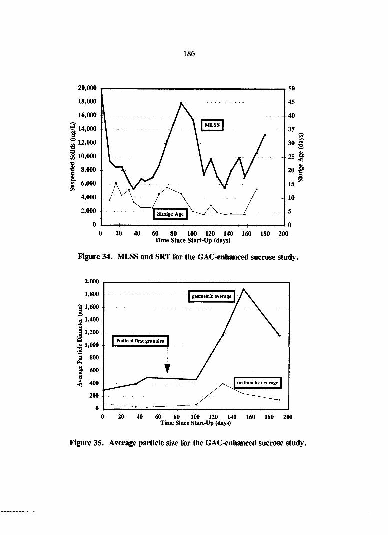
186
20,000
18,000
16,000
14,000
12,000
10,000
_ 8,000 a I 6,000
CA
MLSS
u 25 2P
60 80 100 120 140 160 180 Time Since Start-Up (days)
200
Figure 34. MLSS and SRT for the GAC-enhanced sucrose study.
2,000
1,800
f 1,600 3 b 1.400
I li200
« 1,000
I 800 On I 600
I 400
200
0
Noticed first granules
arithmetic average
20 40 60 80 100 120 140 Time Since Start-Up (days)
200
Figure 35. Average particle size for the GAC-enhanced sucrose study.

187
days less than in the PAC-enhanced ASBR and 45 days less than in the control ASBR.
Initial granulation was also observed in a significantly shorter period of time with the
GAC-enhanced ASBR. The first granules were observed at approximately day 70 in the
GAC-enhanced ASBR, compared to day 90 for the PAC-enhanced ASBR and day 120 for
the control ASBR. Although the GAC-enhanced experiments were not continued to
determine the maximum COD load, the GAC definitely decreased the required start-up
time and may have increased the rate of granulation.
Garnet Enhancement Study
Operational Performance
It was decided to use attachment matrices that did not possess significant adsorptive
capacity to determine whether this property of the PAC and GAC had an effect on the
overall granulation and start-up process. Two matrices, garnet and silica sand, were
chosen. The garnet enhancement study was somewhat more successful than the sand
enhancement study, although neither matrix appeared to have a beneficial effect. This
section presents the data for the garnet study, and the following section presents the data
for the sand enhancement study.
The ASBR was initially seeded with an MLSS concentration of 18,000 mg/L
(MLVSS = 11,000 mg/L) and 2,000 mg/L of garnet sand, which had a specific gravity of
approximately 4.2. Preliminary mixing studies indicated that the garnet sand could be
easily mixed in the ASBR through normal gas recirculation. However, these tests were

188
conducted in pure water. It was impossible to determine whether the garnet was
completely mixed with the biomass after start-up due to the black nature of the biomass.
The ASBR initially received 1 g COD/L/day at a 2-day HRT. After 10 days the
load was increased to 2 g/L/day. The HRT was decreased to 36 hrs after 31 days of
operation, and on day 50 it was decreased to 24 hrs. The COD load at these times were
2.7 and 3.5 g/L/day, respectively (Figures 36 and 37). Below 3.5 g COD/L/day, the
SCOD removal efficiency was in excess of 75%. However, upon decreasing the HRT to
24 hrs (COD load = 3.5 g/L/day), the SCOD removal efficiency dropped to below 40%,
after which it slowly increased to 78% from day 50 to day 110 (Figures 36 and 37).
The volatile acids concentration remained relatively high over the course of this
study. Just prior to increasing the COD load to 2.7 g/L/day, the VFA concentration was
approximately 500 mg/L. After the load was increased to 2.7 g/L/day and later to 3.5
g/L/day, the VFAs increased to over 1,400 mg/L, and were never less than 1,200 mg/L,
indicating that the methanogenic population was not sufficient to degrade the acids
produced by the other bacterial consortia (Figure 38). The reactor pH (Figure 39) was
marginally low over the majority of the study. Although the average pH of the reactor was
approximately 6.8, it fluctuated between 6.6 and 7.0. The COD load was never increased
beyond 3.5 g/L/day due to the relatively poor COD removals (Figure 36), low methane
production (Figure 37), and high VFAs (Figure 38).

189
Soluble Removal
Total Removal
COD Load
20 40 60 80 100 120 Time Since Start-Up (days)
140 160 180
Figure 36. COD removal for the garnet-enhanced sucrose study.
1.6 4.8 relative height of the methane curve to the COD load curve = approximate COD removal based on methane
&1.4 4.2
COD Load 1.2 3.6
3.0
£0 .8 4) i 0.6
2.4 Methane
1.8 Q
"S 0.4 1.2
S 0.2 0.6
0.0 0.0 0 20 40 60 80 100 120 140 160 180
Time Since Start-Up (days)
Figure 37. Methane production for the garnet-enhanced sucrose study.

190
Acids
COD Load
20 40 60 80 100 120 Time Since Start-Up (days)
140 160 180
Figure 38. Volatile acids data for the garnet-enhanced sucrose study.
1 2,400 .o
40 60 80 100 120 140 Time Since Start-Up (days)
Figure 39. Alkalinity and pH data for the garnet-enhanced sucrose study.

191
Solids and Granulation
The MLSS concentration decreased over the first 40 days of operation to 6,100
mg/L (Figure 40). After the COD load was increased to 2.7 and 3.5 g/L/day, a marginal
increase in the MLSS level was observed. After 70 days of operation the MLSS
concentration was approximately 10,000 mg/L. The SRT over this same time decreased
from 16 days (day 40) to approximately 9 days (day 70).
After day 70, the MLSS began to settle less efficiently with a subsequent decrease
in MLSS to 5,000 mg/L and an SRT of only 3 days by day 90. At this point, the HRT of
the system was increased to 2 days to try to increase the solids inventory. After
approximately 2 months of operation at the 2-day HRT, the MLSS increased to over
12,000 mg/L and the SRT increased to approximately 12 days (Figure 40). However, the
COD removal at this point was low (60-65%) and the ASBR was shut down.
Full granulation of the biomass did not occur over the course of the garnet-
enhanced smdy (Figure 41). Although a few granules were detected as early as day 80,
these made up a very small percentage of the total biomass. Over the first 100 days of
operation, the geometric average particle diameter increased slowly to approximately 0.4
mm, although at this point the biomass was visually non-granular. By day 120, the
average size had increase to 0.6 mm. At this point, the biomass was slightly granular to
the unaided eye, but further granulation did not occur.

192
18,000 36
16,000
14,000 s
5? 12,000
§ 10,000 MLSS
on
8,000
I 6,000
cn 4,000
eo "O
2,000
0 20 40 60 80 100 120 140 160 180 Time Since Start-Up (days)
Figure 40. MLSS and SRT for the garnet-enhanced sucrose study.
800
700
a 3600
geometric average g 500
« 400 u
1 £ 300 a OA § 200 >• <
100
arithmetic average
0 20 40 60 80 100 120 140 160 180 Time Since Start-Up (days)
Figure 41. Average particle size for the garnet-enhanced sucrose study.

193
Garnet Effect
The garnet addition to the ASBR did not appear to have any beneficial effects in
terms of granulation or start-up. The high VFA concentration throughout this study
indicates that the methanogenic population never reached sufficient levels. This point is
ftirther substantiated by observation of the poor COD removal and methane production
(Figures 36 and 37, respectively). The non-adsorptive nature of garnet may be responsible
for this effect. In the PAC and GAC studies, the VFAs were fairly moderate (500 - 1,000
mg/L) during start-up, possibly because of adsorption onto the activated carbon.
Adsorption of VFAs onto the carbon, in turn, would enhance methanogenic attachment to
the carbon and maintain high methanogenic populations in the ASBR.
The course of granulation for the garnet study paralleled that of the control reactor
over the first 4 months of operation. There were a few granules present after
approximately 3 months, and over the following month the biomass began to take on a
slightly granular nature. However, the biomass of the PAC and GAC-enhanced ASBRs
were much more granular at an earlier time than that of the garnet-enhanced ASBR. Full
granulation was not observed over the course of this study. However, if given more time,
the biomass may have granulated to a more significant extent.
Silica Sand Enhancement Study
As previously stated, silica sand was also used to enhance granulation and start-up.
The conditions used were identical to those in the garnet study, with the exception that
194
2,000 mg/L of silica sand was used as the attachment matrix. This study was only
conducted for approximately 50 days. Over this period, the COD, VFA, methane, pH,
alkalinity, and solids data closely paralleled that of the garnet study (Figures 42 through
46). After 48 days, the COD removal at a COD load of 2.7 g/L/day was less than 60%
(Figure 42), the VFA concentration had increased to 1,4(X) mg/L (Figure 44), and the
MLSS concentration had decreased to approximately 6,300 mg/L. At this point, owing to
the poor performance of the system and similarity to the garnet-enhanced ASBR, it was
decided to terminate the study in favor of another enhancement method.
Cationic Polymer Enhancement Study
After the experiments were conducted with the various attachment matrices, it was
decided to try an alternative method of granulation enhancement: coagulant addition. It
was hypothesized that by using coagulants, a higher MLSS level could be maintained,
which would be able to degrade higher organic loads at an early stage of start-up. These
high OLRs would result in high biomass production rates, possibly leading to granulation
soon after start-up.
Several coagulants were tested in preliminary experiments to determine which
performed the best in terms of solids separation in the ASBR. These tests were conducted
on operating ASBRs at the end of previous experiments so as not to disturb the natural
progression of those studies. Initially, five different coagulants were tested for use in the
ASBR: a cationic polymer, an anionic polymer, a polyquanternary amine coagulant.
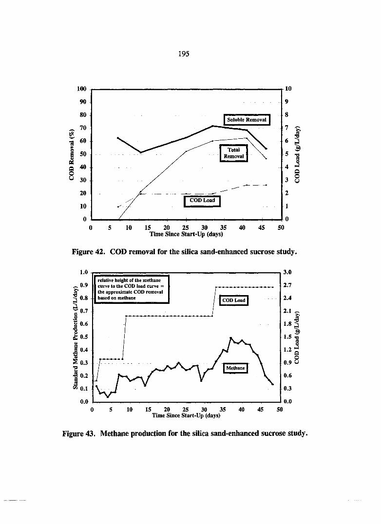
195
100
90
80
70
I I 50 V as fi 40 O
30
20
10
0
j^oluble^emova^
Total Removal
COD Load
10
9
8
•c 6 $
3 5 -a
es
4 ^
•? ® 3 u
2
1
0 15 20 25 30 35
Time Since Start-Up (days) 50
Figure 42. COD removal for the silica sand-enhanced sucrose study.
relative height of the methane curve to the COD load curve = the approximate COD removal based on methane COD Load I
rMethanel
0.0 10 15 20 25 30 35
Time Since Start-Up (days) 40 45
3.0
2.7
2.4
2.1
1.8 t
1.8
1.5 "O
1.2 J O O
0.9 U
0.6
0.3
0.0 50
Figure 43. Methane production for the silica sand-enhanced sucrose study.

196
1,500
1,350
1,200
u CO 1,050
900 ei)
750
§ 5 600 <! 600
u 450
"o > 300
150
0
VFAs
2.5 XI
COD Load
I I
15 20 25 30 35 Time Since Start-Up (days)
Figure 44. Volatile acids data for the silica sand-enhanced sucrose study.
2,500
-3- 2,250 Alkalinity
o 29OOO A
g 1,500
7.0 1 1,250 SB
6.8 a >^1,000 S
750
15 20 25 30 35 Time Since Start-Up (days)
Figure 45. Alkalinity and pH data for the silica sand-enhanced sucrose study.

197
20,000 40
MLSS
18,000 36
0 0 0 5 10 15 20 25 30 35 40 45 50
Time Since Start-Up (days)
Figure 46. MLSS and SRT for the silica sand-enhanced sucrose study.
ferrous chloride, and ferric chloride. Three of these were chosen to be used in actual
granulation enhancement studies. The three, which are discussed in the Expermiental
Procedures section of this document, were the cationic polymer (MAGNIFLOC® 496C,
Cytec Industries), the polyquanternary amine (MAGNIFLOC® 59IC, Cytec Industries),
and ferric chloride. The two polymers had different degrees of cationic charge, and are
differentiated hereafter as the cationic polymer (496C) and the polyDADM coagulant
(591C). The ferric chloride (FeCla- 6H2O) was purchased in powder form from Chemistry
Stores at ISU.

198
The following section presents the data from the cationic polymer (496C)
experiments.
Operational Performance
The most promising results of this research were obtained using the cationic
polymer (MAGNIFLOC® 496C). The ASBR was seeded with approximately 18,000 mg/L
of suspended solids, and initial start-up was conducted at an HRT of 2 days and an OLR of
1 g COD/L/day. The cationic polymer was initially added in liquid form at the rate of 5
mg of polymer per liter of reactor per cycle during the last mixing cycle of the ASBR (just
prior to the settle phase). This dosage was decreased to 1 mg/L/cycle on day 5 after it was
determined that the initial dosage was not necessary for efficient solids separation. After
only 6 days of operation, the HRT was decreased to 1 day and the OLR was increased to 2
g COD/L/day (Figures 47 and 48). Two weeks later the COD load was increased to 3
g/L/day, at which time the SCOD removal efficiency was over 85%. The volatile acids
concentration decreased from 500 mg/L at the 2 g/L/day load to 200 mg/L at the 3
g/L/day load (Figure 49). The pH fluctuated somewhat but averaged between 6.9 and 7.0
over this same time period (Figure 50).
On day 39, the COD load was increased to 4 g/L/day, and by day 61 the ASBR
was treating 6 g COD/L/day at 95% SCOD removal efficiency. At this point the cationic
polymer addition was discontinued to determine whether the reactor would function well
without the benefit of the polymer. After discontinuing the polymer addition, the COD

199
Soluble Removal
Total Removal
stopped polymer addition, day 63 resumed polymer addition, day 123
30
20
10
jjfire^ranulej
i 10
0 0 20 40 60 80 100 120 140 160 180 200
Time Since Start-Up (days)
Figure 47. COD removal for the cationic polymer-enhanced sucrose study.
8.0
relative height of the methane curve to the COD load curve indicates the approximate COD removal based on methane
COD load
tJ 5.0
Methane
t
•o
J § U
60 80 100 120 140 160 Time Since Start-Up (days)
180 200
Figure 48. Methane production for the cationic polymer-enhanced sucrose study.

200
6,000
5,500
5,000
I 4,500
I 4,000
iJ 3,500 ex) §3,000
I 2,500 < « 2,000
I 1,500
1,000
500
0
stopped polymer addition, day 63
resumed polymer addition, day 123
Acids
24
22
20
18
16
14
12
10
8
6
4
2
0
5 d 3 •a a
20 40 60 80 100 120 140 Time Since Start-Up (days)
200
Figure 49. Volatile acids data for the cationic polymer-enhanced sucrose study.
4,000
^3,500
•e 3,000
i 2,500
2,000 6.8 a
M 1,500 5
a 1,000
3 500
20 40 60 80 100 120 140 160 180 200 Time Since Start-Up (days)
Figure 50. Alkalinity and pH data for the cationic polymer-enhanced sucrose study.

201
load was increased to 8 g/L/day and maintained there for 20 days to observe any
detrimental effects. None were apparent and the COD load was increased to 10 g/L/day
on day 100. At this point, the ASBR was achieving 98% SCOD removal (Figure 47),
80% TCOD removal, and had a VFA concentration in the effluent of less than 50 mg/L
(Figure 49). The pH of the ASBR was approximately 6.95 and the alkalinity was more
than 3,000 mg/L, as CaCOj (Figure 50). It thus appeared that the ASBR was operating
under very stable conditions and would be able to handle even higher OLRs.
On day 112 the OLR was increased to 14 g COD/L/day. Over the next two days it
appeared that the system was able to handle the load increase, as was evidenced by the
methane production (Figure 48). However, on day 116 the methane production dropped
significantly. The SCOD removal efficiency decreased to 65% (Figure 47), the volatile
acids concentration increased from less than 50 mg/L to over 3,500 mg/L (Figure 49), and
the pH dropped to 6.7 (Figure 50). The COD load was reduced to 8 g/L/day on day 119
to avoid complete failure of the system.
On day 123, cationic polymer addition was resumed at the rate of 1 mg/L/cycle.
The SCOD removals quickly increased to over 95 % and the VFAs decreased to
approximately 200 mg/L. The COD load was subsequently increased to 10, 12, and 14
g/L/day on days 128, 138, and 146, respectively. The COD removal efficiencies over
these OLRs were in excess of 95%. On day 155, the COD load was increased to 17
g/L/day, which was the highest OLR ever achieved in an ASBR to date. During the first
week at the 17 g/L/day load, methane production was fairly stable and the SCOD removal

202
efficiency was approximately 85% (Figures 47 and 48). After 15 days at this load,
however, the SCOD removal efficiency decreased to approximately 70%. The VFAs
increased to over 3,000 mg/L over this same time (Figure 49), and the pH of the reactor
began to fluctuate significantly and finally decreased to 6.55 on day 164 (Figure 50). At
this point, potassium hydroxide was added to the ASBR to increase the pH to
approximately 6.9, after which the ASBR appeared to achieve a stable, although highly-
stressed, condition. On day 171 the COD load was increased to 20 g/L/day. This load
increase appeared to break the system. COD removals decreased to below 50%, VFAs
increased to 5,500 mg/L, and the pH of the system was unstable and decreased to below
6.4.
Solids and Granulation
The MLSS levels paralleled the operational performance of the ASBR rather
closely. After initial start-up at 18,000 mg/L of suspended solids, the MLSS levels
quickly decreased to 6,000 mg/L after only one week. This was due mainly to the
inefficiency of the cationic polymer to achieve clarification at such a high solids
concentration. The solids tended to form dense mats that were carried up to the liquid
surface due to biogas production during the settle phase. Many of these solids were
washed out in the decanted effluent. This continued for about the first week of operation,
after which the solids settled very well and were not concentrated enough to float due to
gasification. After reaching their minimum concentration of 6,000 mg/L on day 7, the

203
MLSS level increased to over 9,000 mg/L by day 25 and then slowly increased to
approximately 14,000 mg/L by day 70 (Figure 51). Over the first 25 days of operation,
the SRT was generally in excess of 20 days. At about day 34, however, the SRT
decreased to approximately 6 days and fluctuated between 6 and 16 days for the remainder
of the experiment (Figure 51).
Granulation was achieved in an extremely short time in the cationic polymer-
enhanced study (Figure 52). The first granules were observed at approximately day 30, at
which time the geometric average particle diameter was approximately 0.75 mm. By day
60 the average size was more than 1 nmi, and by day 72 the average size had increased to
more than 2.25 mm. The average size remained relatively constant over the next month,
during which the OLR was increased from 6 to 14 g COD/L/day. Granule breakup was
observed after the partial failure of the system at 14 g COD/L/day, and the average size
quickly decreased to 1 mm by day 120. The resumed addition of cationic polymer at this
time did not increase the granule size over the remainder of the study. By the end of the
experiment, the average size was approximately 0.9 mm (Figure 52).
Cationic Polymer Effect
The cationic polymer enhancement had the most beneficial effects on reactor start
up and granulation out of all of the enhancement methods studied. COD removals were in
excess of 95% at a COD load of 6 g/L/day after only 60 days of operation. Granulation
was also enhanced significantly, with the first granules appearing after only 30 days.

204
30,000
stopped polymer addition, day 63 resumed polymer addition, day 123 27,000 36
24,000
5 21,000 en S 18,000 24 MLSS
^ 15,000 T) •f 12,000
UD
9,000
6,000 Sludge Age
3,000
0 20 40 60 80 100 120 140 160 180 Time Since Start-Up (days)
Figure 51. MLSS and SRT for the cationic polymer-enhanced sucrose study.
3,000
2,750
_ 2,500
12,250
I 2,000
I 1,750
« 1,500 U 1 1'250 u 1,000 Be I 750
^ 500
250
0 0 20 40 60 80 100 120 140 160 180
Time Since Start-Up (days)
Noticed first resumed polymer addition, day 123
stopped polymer addition, day 63
loss of biomass due to high COD load (14 g/L/day)
thin line: arithmetic average thick line; geometric average
Figure 52. Average particle size for the cationic polymer-enhanced sucrose study.

205
Almost complete granulation was achieved after 60 days. In addition, it was not necessary
to continue polymer addition after 2 months of operation. COD loads up to 10 g/L/day
were treated to 95 % SCOD removal efficiency without polymer addition, although the
system began to fail when the load was increased to 14 g/L/day. Upon resumed addition
of the polymer, COD loads up to 14 g/L/day were treated to 95% SCOD removal
efficiency. A COD load of 17 g/L/day resulted in reduced efficiency (70%), and at 20
g/L/day the system began to fail.
Examination of the data reveals that the cationic polymer had significant beneficial
effects during the initial start-up period. The polymer maintained the solids in the system
more efficiently than in the other studies resulting in efficient treatment at relatively high
OLRs after only a few weeks of operation. High removal rates results in high biomass
production rates, which is a necessary factor for granulation.
The cationic polymer also had beneficial effects after the system had already
matured. With no polymer addition, the highest COD load attained was 10 g/L/day. With
polymer addition, more than 14 g/L/day could be treated. The most plausible explanation
for this difference is the ability of the polymer to retain solids. At the high COD loads,
biogas production at the end of the cycle was normally still significant, resulting in
turbulent conditions during the settling phase. The cationic polymer helped to settle the
solids in these turbulent conditions. In the reactor with no polymer addition, however,
many of these solids were washed out.

206
PolyDADM Enhancement Study
The other polymer used in these experiments was a polyquanternary amine (59IC),
termed polyDADM for brevity. The polyDADM was slightly less cationic in nature than
the cationic polymer and had a different chemical make-up (Experimental Procedures
section).
Operational Performance
The ASBR in the polyDADM enhancement study was initially seeded with 18,(X)0
mg/L of suspended solids and operated at an HRT and OLR of 2 days and 1 g
COD/L/day, respectively. The polyDADM coagulant was added during the last mixing
cycle just prior to the settle phase at a rate of 5 mg/L/cycle. After 5 days of operation, the
coagulant dosage was decreased to 2.5 mg/L/cycle, but was increased back to 5
mg/L/cycle 2 days later due to poor clarification at the lower dosage. The coagulant
dosage was maintained at 5 mg/L/cycle until day 60, when it was again reduced to 2.5
mg/L/cycle. On day 70, the dosage was reduced further to 1 mg/L/cycle.
After 6 days of operation at 1 g COD/L/day (2-day HRT), the COD load was
increased to 2 g/L/day by decreasing the HRT to 1 day and maintaining a constant influent
COD concentration of 2 g/L. On day 39, the COD load was increased to 3 g/L/day,
although the SCOD removal efficiency was only 67% (Figures 53 and 54). The volatile
acids concentration over the first 39 days was relatively constant at 500 mg/L, and the pH
was between 6.9 and 7.0 (Figures 55 and 56).

207
Switched to cationic •J
^olubl^Remov^J
Total Removal
COD Load
4-
20 40 60 80 100 120 140 160 180 200 Time Since Start-Up (days)
Figure 53. COD removal for the polyDADM-enhanced sucrose study.
relative height of the methane curve to the COD load curve indicates the approximate COD removal based on methane
switch to cationic polymer, day 84
COD Load
Methane I
60 80 100 120 140 Time Since Start-Up (days)
200
Figure 54. Methane production for the polyDADM-enhanced sucrose study.
208
2,500
2,250 switched to cationic
-2,000
S 1.750
J 1,500
I 1,250
3 1,000 < u = 750 S > 500
60 80 100 120 140 160 180 200 Time Since Start-Up (days)
Figure 55. Volatile acids data for the polyDADM-enhanced sucrose study.
5 3,500
€ 3,000
i 2,500
2,000 6.8 3
M 1,500 5
a 1.000
3 500
20 40 60 80 100 120 140 160 180 200 Time Since Start-Up (days)
Figure 56. Alkalinity and pH data for the polyDADM-enhanced sucrose study.

209
After the increase to 3 g COD/L/day on day 39, the VFA concentration increased
to 1,000 mg/L at day 55, while the SCOD removal efficiency decreased to 58% (Figures
55 and 53, respectively). The pH of the system dropped over this time to an average of
6.7 (Figure 56). On day 72, the COD load was increased to 4 g/L/day to try to push the
system somewhat, but the COD removal efficiency dropped to below 50% and the VFAs
increased to over 1,700 mg/L. The COD load was decreased to 3 g/L/day to avoid
system failure.
Since the polyDADM-enhanced ASBR was performing much worse than the
cationic polymer-enhanced ASBR, it was decided on day 84 to switch the coagulant from
polyDADM to cationic polymer to determine whether the stressed conditions could be
alleviated. Improvement of the system would also lend support to the beneficial effects
observed for the cationic polymer-enhanced test that was being conducted in parallel.
Almost immediately the methane production increased to a limited extent after switching
coagulants (Figure 54). The SCOD removal increased to over 70% by day 95 (Figure 53),
and the VFAs decreased to 600 mg/L (Figure 55). The pH of the system also increased to
between 6.8 and 7.0 and remained within this range throughout the remainder of the
experiment (Figure 56).
On day 110 the COD load was increased to 4 g/L/day and on day 130 it was ftirther
increased to 5 g/L/day. The SCOD removal efficiency during this time remained at
approximately 70%and the VFAs fluctuated between 1,000 and 1,200 mg/L. On day 155
the COD load was increased to 6 g/L/day and the SCOD removal efficiency increased to

210
over 80%. Upon further increase of the COD load to 8 g/L/day (day 170), the COD
removal efficiency decreased to below 60% (Figure 53).
Solids and Granulation
The MLSS levels decreased from 18,000 mg/L to a minimum of 5,200 mg/L
during the first 25 days of operation (Figure 57). Over the next 50 days the solids level
slowly increased to approximately 10,000 mg/L on day 75. During the remainder of the
experiment the solids level flucmated marginally but was normally around 9,000 mg/L.
The SRT changed drastically over the first 70 days of operation, with a high of 57 days
(day 58) and a low of 6 days (day 12). After the switch to cationic polymer on day 84,
the SRT remained fairly constant with an average of 10 days. After the COD load was
increased to 6 g/L/day, however, the SRT fell below 5 days (Figure 57).
The biomass never fully-granulated in the polyDADM study (Figure 58). The
geometric average particle diameter increased gradually from 0.1 nmi to 0.35 mm during
the first 100 days of operation. At the end of the study, the average diameter again began
to increase, and the biomass visually appeared to be granulating to a limited extent.
However, the individual particles were still quite small and obvious granulation was not
apparent (Figure 58).
211
20,000
18,000 switch to cationic
16,000
a 14,000 B,
12,000
10,000 MLSS
•a 8,000
g 6,000
4,000
60 80 100 120 140 Time Since Start-Up (days)
200
Figure 57. MLSS and SRT for the polyDADM-enhanced sucrose study.
500
450
-^400 3 I. 350 (y
1
at 2S0
I 200
1.5. V 100
50
0 0 20 40 60 80 100 120 140 160 180 200
Time Since Start-Up (days)
I switch to cationic
arithmetic average I
Figure 58. Average particle size for the polyDADM-enhanced sucrose study.

212
PoIyDADM Effiect
The polyDADM coagulant appeared to have a non-stimulatory (if not inhibitory)
effect on ASBR start-up and granulation. Although COD removal and methane production
occurred, it did not reach the levels achieved in most of the other experiments.
Additionally, the average particle size actually lagged behind that of the control smdy,
indicating that the polyDADM coagulant may have inhibited granule formation. The
switch to cationic polymer was able to increase COD removals, but granulation of the
biomass did not occur to a significant extent.
It seems likely that the chemical nature of the polyDADM coagulant may have
inhibited the methanogens, since sucrose conversion to acids was observed but methane
production was low. An alternative explanation is that the chemical nature of the
polyDADM selected for different species of methanogens than those selected for by the
cationic polymer. This latter possibility would account for only a marginal increase in
performance after the switch to the cationic polymer. There may have been insufficient
numbers of the desired methanogens present prior to the switch, so that even when the
polyDADM was removed from the system the desired methanogens were simply not
present.
A third possibility is that the polyDADM suppressed the pH enough to effect the
methanogens. Prior to the switch to cationic polymer, the pH of the system was
consistently between 6.6 and 6.7, even when additional buffering capacity was provided

213
(Figure 56). After switching to the cationic polymer, however, the pH increased to a
constant value between 6.8 and 7.0, which is more suitable for most methanogenic species.
Ferric Chloride Enhancement Study
Ferric chloride (FeClj- 6H2O) was also used for enhancement of start-up and
granulation. Ferric chloride was selected because of its common use in drinking water
treatment as a coagulant. Iron is also a necessary trace metal and has been implicated by
some authors to be limiting in some anaerobic treatment applications [58, 115, 126, 138].
Operational Performance
The ferric chloride (FeCl3)-enhanced ASBR was seeded with 18,000 mg/L of
suspended solids and initially operated at an HRT an OLR of 2 days and 1 g/L/day,
respectively. The FeClj dosage applied to the ASBR was 5 mg/L/cycle (as Fe) throughout
the experiment. After 6 days of operation the COD load was increased to 2 g/L/day and
the HRT was decreased to 1 day. The SCOD removal efficiency was approximately 60%
at this time and the TCOD removal was slightly less at 55% (Figure 59). Methane
production indicated a lower COD removal efficiency, although methane production was
inconsistent over the course of the experiment (Figure 60).
The COD load was never increased beyond 2 g/L/day during the entire course of
the experiment due to the extremely low COD removals observed. At day 35, the SCOD
removal efficiency was 40% and by day 55 it had decreased to 34% (Figure 59). The

214
100
90
80
^ 70 #
I 50
Q 40 O y 30
20
10
0
I COD Load f
rSoIubl^emovall
i I ! ! I I f—H ill I
10 15 20 25 30 35 40 45 50 55 60 Time Since Start-Up (days)
10.0
9.0
8.0
7.0
6.0
5.0
4.0
3.0
2.0
1.0
0.0
I w •a es o
Q O U
Figure 59. COD removal for the ferric chloride-enhanced sucrose study.
1.0
0.9
I 0.8
^0.7 a _o
I 0.6
1 (t 0.5 0) a 5 0.4
0.3
0.2
0.1
0.0
tfl
relative height of the methane curve to the COD load curve = approxiamte COD removal based on methane
JcOD^^
Methane
20 25 30 35 40 Time Since Start-Up (days)
3.0
2.7
2.4
2.1
1.8 t
1.8
1.5 "O 9
1.2 S Q O
0.9 u
0.6
0.3
0.0
Figure 60. Methane production for the ferric chloride-enhanced sucrose study.

215
VFAs reached a low of 650 mg/L on day 23, but increased steadily thereafter to 1,000
mg/L on day 55 (Figure 61). The pH of the system was always between 6.8 and 7.0, and
the alkalinity averaged 1,300 mg/L as CaC03 (Figure 62). This experiment was
terminated after 55 days of operation due to the obvious poor performance of the reactor.
Solids and Granulation
The solids level decreased from its initial value of 18,000 mg/L to 6,200 mg/L at
day 10. A marginal increase in the MLSS level occurred over the remainder of the
experiment, but it never exceeded 7,800 mg/L (Figure 63). The SRT of the system was
always in excess of 15 days and normally was greater than 30 days. This latter
observation is a point of confusion and is in direct contrast to normal anaerobic treatment
theory. It is generally thought that longer SRTs create stable conditions for anaerobic
treatment. In fact, the basis of the anaerobic filter is the efficient retention of biomass and
long SRT attainable. However, in these experiments shorter SRTs appear to be beneficial
to start-up and granulation in the ASBR.
Granulation did not occur over this short experiment (Figure 64). The majority of
the biomass was in the form of small, pin-point floes that settled unusually well. The
efficient clarification during this experiment was also evidenced by the similar SCOD and
TCOD removal efficiencies (Figure 59). That is, few solids were lost in the effluent. This
fact, together with the small increase in MLSS, suggests that the biomass production rates
were very low.

216
Acids 4.0 >>
15 20 25 30 35 40 45 Time Since Start-Up (days)
Figure 61. Volatile acids data for the ferric chloride-enhanced sucrose study.
1,600
Alkalinity tr 1,400
I 1,200
I 6.6 s
u 600 E
•f 400
3 200
0 5 10 15 20 25 30 35 40 45 50 55 60 Time Since Start-Up (days)
Figure 62. Alkalinity and pH data for the ferric chloride-enhanced sucrose study.

217
20,000 rlOO
18,000 90
16,000
14,000 OJD ' E r 12,000
80
60
10,000
8,000
MLSS I 6,000
4,000
2,000
0 5 10 15 20 25 30 35 40 45 50 55 60 Time Since Stait-Up (days)
Figure 63. MLSS and SRT for the ferric cliloride-enhanced sucrose study.
400
350
250 I geometric average
4! 200
(2 150 o
§ 100 arithmetic average
0 5 10 15 20 25 30 35 40 45 50 55 60 Time Since Start-Up (days)
Figure 64. Average particle size for the ferric chloride-enhanced sucrose study.

Ferric Chloride Effect
It is obvious after examining the data from this experiment that the ferric chloride
had an inhibitory effect on the start-up and granulation of the ASBR. Perhaps the most
plausible explanation is that the ferric ions contributed by the ferric chloride were reduced
to ferrous ions in the anaerobic environment, and subsequently precipitated with sulfide to
form ferrous sulfide (FeS). Ferrous sulfide is relatively insoluble in water and is generally
present in pin-point floes. Also, if the iron is present at high concentrations, the FeS
formed may scavenge the system of the majority of the available sulfur. This would result
in inhibition of the system due to a limiting supply of sulfur, which is a necessary nutrient
for life. These two points correlate well with the observed ASBR performance.
Beef Extract/Glucose Experiments
Completion of the previously presented experiments yielded several enhancement
methods capable of improving the start-up and granulation in ASBRs treating a sucrose
wastewater. However, since sucrose was used as the sole carbon source in all of the
experiments to this point, it was decided to use a different substrate in similar experiments
to determine what effect (if any) the type of substrate had on start-up and granulation
parameters. The substrate chosen for study was a combination of beef extract and glucose,
combined in a 50/50 ratio based on COD contribution. The characteristics of the beef
extract are given in the Experimental Procedures section of this document. Glucose was
purchased in powder form from Chemistry Stores at ISU.

219
Due to the long nature of these experiments, the best enhancement method from the
sucrose experiments was chosen for study in the beef extract/glucose experiments, namely,
cationic polymer enhancement. A control ASBR was also operated in parallel to the
cationic polymer-enhanced ASBR. The beef extract contained a high amount of protein
(12.9% by weight) and fat (13.5% by weight) in addition to a significant amount of
carbohydrates (24.0% by weight). It was anticipated that the protein content of the beef
extract would eliminate some of the requirement for alkalinity addition. This point was
apparent throughout the study and is evidenced by the lower sodium bicarbonate addition
required to maintain optimum pH conditions (compared to the sucrose experiments, see
Tables 13 and 14 in the Experimental Procedures section). It was further anticipated that
the high fat content may cause problems due to floating biomass. This latter point is
addressed in the following paragraphs.
Control Study
Operational Performance
The control ASBR was initially seeded with 25,000 mg/L of suspended solids
(MLVSS = 15,000 mg/L). The HRT and OLR were set at 2 days and 1 g COD/L/day,
respectively. Polymer was not added to the control reactor. After 7 days of operation, the
HRT was decreased to 1 day and the OLR was increased to 2 g COD/L/day. On day 30
the HRT was increased to 2 days due to poor performance and maintained at 2 days until
day 47 (Figures 65 and 66). At day 60 the COD load was increased from 2 to 3 g/L/day,
220
£ > o E <u ei a o U
100
90
80
70
60
50
40
30
20
10
0
Soluble Removal
Total Removal
COD Load
20
18
16
. 1 4 ^
-12
10 T) cs
• 6 8
4
2
0 10 20 30 40 50 60 70 80 90 100 110 Time Since Start-Up (days)
120
Figure 65. COD removal for the beef/glucose control study.
2.2 r 6.6
^2.0 i 5 1.8 d <d 1.6
6.0
5.4
4.8 "i*
4.2 -3
3.6 •o
3.0 §
2.4 9
•S 1.4
0.8
0.6 1.8
0.4 1.2 Methane
^ 0.2 0.6
0.0 0.0
Load
Noticed slight granular nature
relative height of the methane curve to the COD load curve = approximate COD removal based on methane
t
•o
10 20 30 40 50 60 70 80 90 100 110 120 Time Since Start-Up (days)
Figure 66. Methane production for the beef/glucose control study.

221
even though the COD removal efficiency was only 60%. The VFA concentration reached
a maximum of 1,600 mg/L on day 30 but subsequently decreased to 500 mg/L by day 60
(Figure 67). The alkalinity and pH remained relatively constant at 2,750 mg/L and 6.90 to
7.1, respectively, throughout the study (Figure 68).
After 18 days at a COD load of 3 g/L/day the COD removal efficiency and methane
production began to improve. On day 78 the COD load was increased to 4 g/L/day and
maintained at that level until day 100. The SCOD removal efficiency was approximately
70% at the 4 g/L/day COD load (Figure 65). On day 101 the COD load was increased to
6 g/L/day, resulting in decreased COD removals and increased VFA concentrations
(Figure 65 and 67).
Solids and Granulation
Figures 69 and 70 present the solids and granulation data from the control
experiment. The MLSS level decreased from 25,000 mg/L at day zero to 7,500 mg/L at
day 7. The MLSS level remained relatively constant at 7,000 mg/L until day 80 at which
time it briefly decreased to 4,000 mg/L before increasing again to 7,000 mg/L (Figure 69).
The SRT likewise decreased from 69 days to 7 days during the first 21 days of operation.
After this point the SRT fluctuated, reaching 26 days on day 40 and then decreasing to 8
days by the end of the experiment (day 109).
The geometric average particle size gradually increased over the course of the
experiment to approximately 0.5 mm by day 109 (Figure 70). At this point the biomass

222
2,000
U 1,400
B 1,000
S 800
S 600 n > 400
COD Load
1-
30 40 50 60 70 80 90 Time Since Start-Up (days)
100 110 120
Figure 67. Volatile acids data for the beef/glucose control study.
3,000
2,700 Alkalinity
2,400
U 2,100
1,800
7.0 a
1,200 •a
900
6.8 cf
0 10 20 30 40 50 60 70 80 90 100 110 Time Since Start-Up (days)
Figure 68. Alkalinity and pH data for the beef/glucose control study.

223
32,000 r80
28,000 70
^ 24,000
OS
S 20,000
60
16,000
DC •c a 12,000
w 8,000
4,000 10
0 10 20 30 40 50 60 70 80 90 100 110 120 Time Since Start-Up (days)
Figure 69. MLSS and SRT for the beef/glucose control study.
600 Noticed first granules 550
^500
J, 450
I 400 geometric average
350
« 300
v 200
150
100 arithmetic average
0 10 20 30 40 50 60 70 80 90 100 110 120 Time Since Start-Up (days)
Figure 70. Average particle size for the beef/glucose control study.

224
had a slight granular nature but did not approach the granular character observed in the
sucrose experiments. The first granules were observed at approximately day 60.
After approximately day 30 the biomass settling characteristics changed
significantly. Prior to this the biomass settled normally, comparable to the biomass
observed in the sucrose experiments. However, as the experiment progressed the biomass
began to float to the top of the ASBR during the settle phase, most likely due to high fat
concentrations in the reactor. (Alternatively, it is also possible that the high protein
content of the beef substrate caused the floating biomass. Protein has hydrophobic and
hydrophilic regions and may act similarly to soap or fat molecules under certain
conditions. The fat, however, is a more likely suspect due to the fact that other
proteinaceous wastes have been treated in the ASBR without causing the biomass to float.)
For this reason, the decant port was relocated to one of the bottom ports on the ASBR.
This phenomenon reached an extreme by day 50 at which time the entire biomass
population floated to the top of the ASBR during the settle phase. This condition
continued for the remainder of the experiment. This would not have caused a serious
problem except that as the biomass began to granulate, the heavier biomass particles tended
to sink during the decant phase and were washed out of the reactor. This observation may
have lead to inhibition of granulation since the heavier (and better settling) particles were
washed out of the ASBR rather than being retained, as is normally the case.
The phenomenon of biomass flotation due to fat accumulation must be studied
further. This obviously presents serious difficulties in developing a granular biomass. In

225
addition, the biomass caught in the floating layer is essentially unavailable for substrate
degradation since in seldom contacts the liquid portion of the reactor. This latter point was
most probably the cause of the relatively poor COD removals observed throughout this
smdy.
Cationic Polymer Enhancement Study
Operational Performance
An ASBR enhanced with cationic polymer was operated in parallel with the control
reactor. The cationic polymer-enhanced ASBR was seeded with 25,000 mg/L of
suspended solids (MLVSS = 15,000 mg/L) and operated at an HRT and OLR of 2 days
and 1 g COD/L/day, respectively. The cationic polymer dosage was initially 2
mg/L/cycle. After 1 week of operation the HRT was decreased to 1 day, the COD load
was increased to 2 g/L/day, and the polymer dosage was reduced to 1 mg/L/cycle. The
ASBR was operated under these conditions for two weeks, during which the SCOD
removal efficiency was in excess of 80% (Figures 71 and 72) and the volatile acids
concentration averaged 250 mg/L (Figure 73). The alkalinity and pH were consistent
throughout the study. The alkalinity increased gradually over the course of the study from
2,400 mg/L to 3,200 mg/L, as CaCOj. The pH fluctuated marginally but remained within
6.8 and 7.2 throughout the experiment (Figure 74).
On day 22 the COD load was increased to 3 g/L/day and the SCOD removal
efficiency increased to over 85 % while the VFA concentration remained at 250 mg/L, as
226
30 40 50 60 70 80 90 100 110 120 Time Since Start-Up (days)
Figure 71. COD removal for the cationic polymer-enhanced beef/glucose study.
relative height of methane curve to the load curve = approximate COD removal based on methane
Methane V 1.0
0 10 20 30 40 50 60 70 80 90 100 110 120 Time Since Start-Up (days)
Figure 72. Methane production for the cationic polymer-enhanced beef/glucose study.

227
2,250
2,000
U 1,750
J 1,500
5 1,250
S 1,000 <!
VFAs
10 20 30 40 50 60 70 80 90 100 110 120 Time Since Start-Up (days)
Figure 73. Volatile acids data for the cationic polymer-enhanced beef/glucose study.
4,000 8.0
3,600 - 7 . 8
3,200 7.6 Alkalinity
2,800 7.4
2,400 7.2
2,000 7.0
>.1,600 •a 1 1,200
6.8
6.6
800 6.4
400 6.2
0 6.0 0 10 20 30 40 50 60 70 80 90 100 110 120
Time Since Start-Up (days)
Figure 74. Alkalinity and pH data for the cat. polymer-enhanced beef/glucose study.

228
acetic. On day 39 the COD load was increased to 4.5 g/L/day. At this point the biomass
began to float as in the control experiment. This observation is discussed further below.
After the COD load was increased to 4.5 g/L/day, the SCOD removal efficiency decreased
to 62% and the VFA concentration increased to 1,700 mg/L due to loss of biomass
(Figures 71 and 73). At this point the COD load was decreased to 3 g/L/day to avoid
failure of the system. On day 60 the COD load was increased again to 4 g/L/day. The
SCOD removal efficiency increased to 80% and the VFA concentration decreased to below
100 mg/L. On day 71 the COD load was increased to 5 g/L/day and the SCOD removal
efficiency increased further to 90% (Figure 71).
On day 79 the COD load was increased to 6 g/L/day resulting in a decreased SCOD
removal efficiency which leveled off at approximately 70%. The VFA concentration
increased from 250 mg/L to almost 2,000 mg/1 before leveling off at 1,300 mg/L on day
95. On day 98 the COD load was increased to its final value of 8 g/L/day, resulting in
decreased COD removals and increased VFA concentrations (Figure 71 and 73,
respectively).
Solids and Granulation
Figures 75 and 76 present the MLSS and particle size analyses, respectively, for the
cationic polymer-enhanced ASBR study. The MLSS level decreased from 25,000 mg/L to
a relatively constant value of 11,000 mg/L after 20 days of operation. As the COD load
was increased from 2 to 3 g/L/day, the biomass began to granulate, with the first granules

229
30,000
27,500
25,000
^ 22,500
u 20,000 E M 17,500
15,000
•a 12,500 e 110,000
^ 7,500
MLSS
40
30 40 50 60 70 80 90 Time Since Start-Up (days)
100 110 120
Figure 75. MLSS and SRT for the cationic polymer-enhanced beef/glucose study.
1,000
900
800
700
geometric average
300
< 200 arithmeticic average
100
0 10 20 30 40 50 60 70 80 90 100 110 120 Time Since Start-Up (days)
Figure 76. Average particle size for the cationic polymer-enhanced beef/glucose study.

230
noticed on day 39 (Figure 76). Also, at this point, the biomass began to float. A
significant amount of biomass washed out of the ASBR and the MLSS level decreased to
5,000 mg/L by day 42. After relocating the effluent port to a lower level on the ASBR,
the MLSS level increased to 12,500 mg/L over the next 25 days (Figure 75). During this
same time the SRT of the system increased from 7 days to over 60 days. This increasewas
due to the compact nature of the floating biomass. The combined action of the fat and
polymer created a fairly dense floating layer at the top of the ASBR. Very few solids were
lost during the decant operations, resulting in an increasing MLSS concentration and SRT.
At day 80 another loss of biomass occurred. This loss was due to the increasing
granular nature of the biomass. The action of flotation was counteracted by the settling
characteristics of the granules, which resulted in a dispersed, or suspended biomass
throughout the ASBR. Many of the granules were washed out during this time, leaving
behind the floating biomass layer at the top of the reactor.
Granulation was observed in the cationic polymer study. As previously stated, the
first granules were observed after only 39 days of operation. At this point the geometric
average particle size was approximately 0.45 mm. By day 50 the average size had
increased to 0.7 mm. During the second period of biomass washout (day 80), however,
many of the larger granules were lost and the average size decreased to 0.5 mm. By the
end of the experiment the average size was again increasing and was nearly 0.9 mm.

231
Cationic Polymer EfTect
As was observed in the sucrose experiment, the cationic polymer has significant
beneficial effects on the start-up and granulation of the ASBR. The COD load and COD
removal efficiency were significantly higher at any given time in the cationic polymer
experiment as compared to the control. The progress of granulation was also enhanced by
polymer addition.
As stated earlier, the subject of anaerobic degradation of fat must be further
addressed. The fat content of the beef extract caused serious difficulties in the operation of
the ASBR. In practice it appears that removal of fat from the wastewater stream would be
advantageous. Alternatively, the biological degradation of fat in anaerobic reactors would
preclude the necessity of fat removal with the added benefit of increased methane
production.
Summary of Enhancement Studies
The overall effects of the enhancement methods used in this research were varied,
both among the specific enhancement techniques and between the two substrates used. The
best method employed was the addition of the cationic polymer during the first two months
of operation. GAC and PAC also had stimulatory effects on start-up and granulation,
though most probably through different mechanisms. Table 27 presents a summary of
these experiments in terms of the required time to attain specific COD loading rates and
granulation.

232
Table 27. Start-up and granulation summary. Time Required for Objective to be Attained
Substrate Enhancement 3
g/L/day 4
g/L/day 5
g/L/day 8
g/L/day 14
g/L/day first
granules full
granulation
sucrose none 90 100 107 135 ... 130 140+
sucrose PAC 63 80 110 130 150 90 100+
sucrose GAC 30 38 62 88 ... 71 80+
sucrose garnet^ 48 ... ... ... ... 75 ...
sucrose sand ... — ... ... ... ... ...
sucrose cationic'' 29 39 59 64 110 31 55 +
sucrose polyDADM'^ 39 66 130 170 ... 101 ...
sucrose FeClj ... ... ... ... ... ... ...
beef/glucose none 61 80 100 ... ... 61 ...
beef/glucose cationic 21 35 43 107 ... 39 90+
" The granules observed in this reactor were different than those from other experiments. It is believed that these granules were inorganic particles, since further granulation of the biomass did not occur.
'' The COD load was subsequently increased to 6 g/L/day on day 61. ' The COD load had to be decreased back to 3 g/L/day on day 81 due to poor performance; switched to cationic on day 84.
The enhancement mechanism of the GAC and PAC were probably similar. Both
materials have a high adsorption capacity and probably adsorbed a significant amount of
volatile acids during the start-up phase. This would have had two stimulatory effects: (1)
Volatile acids are often present at significant concentrations during start-up due to the more
rapid growth rates of the acidogenic and acetogenic bacteria as compared to the
methanogens. High initial VFAs may inhibit the growth of the desired methanogens that
have a relatively low value for acetate. Through adsorption on to activated carbon the
bulk liquid concentration of VFAs is reduced, thereby creating more favorable conditions
233
for the desired methanogens. And (2) the activated carbon with adsorbed VFAs provides
an ideal site for bacterial attachment. The adsorptive capacity of activated carbon is
normally easily inhabited by bacteria. However, with an abundant supply of food the
surface provides an even better site for bacterial growth.
GAC appears to have an advantage over PAC, especially during the first few
weeks after start-up. Although PAC has a larger surface area per mass of carbon, its small
size does not allow for efficient sedimentation in the solids-concentrated environment of
the ASBR. GAC, however, settles rapidly and is retained in the reactor more efficiently.
Although the lower surface area of GAC may not build up as high of a concentration of
biomass per mass of carbon (compared to PAC), the biomass that does become attached
will be retained in the reactor.
The enhancement mechanism of the cationic polymer is necessarily different from
that of activated carbon. During the start-up with cationic polymer enhancement the
effluent from the ASBRs contained few solids (after the initial washout of biomass during
the first week of operation). Therefore, the bacteria that was initially present in the seed
biomass were retained within the reactor more efficiently than in other studies. By
artificially maintaining high MLSS concentrations during the critical start-up period, COD
removals were improved and the biomass concentrations could increase more rapidly.
Although not explicitly proven, the cationic polymer also may have facilitated cell contact
among adjacent bacteria. Since the surface charge of most bacteria is generally negative,
the positive charge of the cationic polymer should act to bridge bacteria together. As more

234
bacteria began to come in contact with each other, granulation naturally progressed until
further addition of the polymer was unnecessary.
Specific Methanogenic Activity Experiments
Background and Theory
Several specific methanogenic activity tests were conducted during this research.
As previously stated, the GAC-enhanced ASBR was used extensively for this purpose.
The PAC-enhanced and garnet-enhanced ASBRs were also used to a lesser extent to
determine typical SMAs of the biomass. Both flocculent and granular biomass were used
in the SMA tests. Sucrose and acetate were used individually as the substrate, and
nutrients, trace metals, and buffering compounds were added as required (Experimental
Procedures section). Sucrose and acetate were used in separate SMA tests to try to
determine bacterial arrangement within the granule structure. Granule structure was
discussed in the Literature Review section of this document and is briefly reviewed here.
There are generally two different bacterial arrangements normally found in
granules; layered and non-layered (Figures 77 and 78, respectively). Layered granules
generally have three fairly distinct zones of bacteria. The outer zone often consists of a
heterogeneous consortia of many bacterial species and morphologies. The inner zone is
usually a fairly homogenous core of rod-shaped bacteria, often cited as Methanothrix-type
cells. The middle layer is a transition zone between the two extremes, and consists mainly
of acetogenic and methanogenic bacteria which exist in a symbiotic relationship (Figure

235
Heterogeneous population of all bacterial groups
Acetogens and
Methanogens
Mainly Methanogens
Direction of Substrate^
Flow
rt«S»V*
Figure 77. Idealized granule exhibiting a layered structure.
population of all bacterial groups
^ .%,••• ,• % ,• •• ,•.• *. ,• •, / %v '.Tt— •/. •/, •,*. •/. •/.
if.* •* • .* • .* • .* •»• .• • ,• *• •" *• .* *• .• *•
••^•vV•V^vVv^V;i^ */• *1 *'/' •.*•
*• *•.* •••• •• V •> ••> •• V % V *. V •
• •/. •.*. •. •*,* .*.• *
No uniform direction of substrate Flow
• i*. •••• •.*. •.% •/. •.*. •/. •/. •/. - A
Figure 78. Idealized granule exhibiting a non-layered structure.
236
77). One theory is that complex substrates (sucrose) are converted to volatile acids by the
outer-zone bacteria. The volatile acids are then immediately used by the nearby acetogenic
bacteria in the middle zone. Hydrogen and carbon dioxide produced by the acetogens are
rapidly converted to methane by the methanogens present in the middle layer. Acetate
produced by the acetogens diffiises into the core of the granule where the acetoclastic
methanogens convert it to methane and carbon dioxide.
Non-layered granules generally consist of a heterogeneous consortia of bacteria
throughout the entire structure with no obvious zones of homogeneity (Figure 78).
Alternatively, non-layered granules may also consist of a homogeneous population of only
one or two bacterial species, as may be the case for granules developed on simple
substrates such as acetate. In heterogeneous non-layered granules there is no obvious
direction of intermediate flow as was discussed for layered granules. Rather, intermediate
degradation products may diffuse in any direction and methane production may
theoretically occur throughout the granule.
The layered or non-layered structure of a granule may be tentatively elucidated by
conducting SMA tests with different substrates. For example, consider a granule with a
layered structure which is fed sucrose as its sole carbon source. The sucrose is degraded
to acids in the outer layer, followed by acetogenesis and methanogenesis in the middle and
inner layers, respectively. The progression of sucrose degradation to acids and finally to
methane can occur rapidly because of the thermodynamic advantage of granule biomass
over flocculent biomass. However, now suppose the same layered granule is fed a simple

237
substrate such as acetate. The majority of the acetoclastic methanogens are located in the
center of the granule, and, therefore, the acetate must diffuse into the granule before
methanogenesis can occur. Stated differently, methane production (SMA) may actually
occur more rapidly from sucrose than from acetate in a layered granule.
Now consider a granule with a non-layered structure. Since the methanogenic
organisms are located throughout the granule, methanogenesis from acetate should
theoretically occur more rapidly than methanogenesis from sucrose due to the fewer
intermediate steps. Therefore, the SMA of the biomass fed acetate should be greater than
(or at least equal to) the SMA from sucrose degradation.
Specific Methanogenic Activity Results
Sucrose Tests
The results of the various SMA experiments are presented in Table 28. Eight tests
were conducted with sucrose as the substrate: 2 tests with flocculent biomass (GAC and
garnet studies) and 6 with granular biomass (GAC and PAC tests). The granular tests
were conducted with biomass at various stages of granulation. The GAC series of
experiments especially provided a time-dependent progression of SMA from flocculent
biomass (day 65) to slightly granular (day 93) to fully granular (days 133, 135, and 190).
Examination of the GAC SMA data from day 65 to 93, an obvious increase
(doubling) in activity is observed, coinciding with granulation of the biomass in the GAC-
enhanced ASBR. After the biomass had fully granulated the SMA increased still further

238
Table 28. Summary of specific methanogenic activity experiments.
Experiment
Time Since Start-Up (days)
Biomass Type
SMA" (ml/g/min)''
SMA (/xmoles/g/min)'
SttcrQst
Garnet 83 flocculent 0.12 6.70
GAC 65 flocculent 0.07 3.13
GAC 93 granular 0.16 7.14
GAC 113 granular 0.22 9.82
GAC 135 granular 0.19 8.48
GAC 190 granular 0.17 7.59
PAC 158 granular 0.13 5.80
PAC 228 granular 0.14 6.25
GAC 76 flocculent 0.09 4.02
GAC 195 granular 0.19 6.70
PAC 169 granular 0.02 0.89
• Specific methanogenic activity. '• Units are milliliters of methane per gram of volatile suspended solids per minute (@ STP). ' Units are micromoles of methane per gram of volatile suspended solids per minute (@STP).
239
from 0.16 mL CHJg MLVSS/min at day 93 to 0.22 mL CH^g MLVSS/min at day 113.
Beyond this point the SMA of the GAC-enhanced biomass decreased slightly to 0.19 mL
Ciajg MLVSS/min on day 135 and 0.17 mL CHJg MLVSS/min by the end of the GAC
study (day 190). Figure 79 presents the data for the GAC SMA tests (sucrose) in graphical
form.
Figure 80 shows a comparison of the SMA curves for biomass developed in two
separate studies. The granular data are from the GAC-enhanced ASBR on day 113 of that
experiment. The flocculent data are from the garnet-enhanced ASBR on day 83. Both of
the biomass samples were mature, but the activity of the granular biomass was
considerably higher than that of the flocculent biomass. The granular biomass from the
PAC study had a slightly lower SMA than that of the GAC study. This observation may
have been due to the extremely high MLSS levels of the PAC-enhanced ASBR (up to
27,000 mg/L). The biogas-recirculation mixing may not have been sufficient to
completely-mix the ASBR during the SMA test, which would have resulted in
underestimating the SMA of the biomass.
Acetate Tests
Results of the SMA tests using acetate as a substrate are inconclusive concerning
their relationship to granule structure. The SMA on acetate of the GAC-enhanced biomass
increased significantly after granulation had occurred in the ASBR. This can be explained
due to the increase in numbers of methanogenic organisms compared to the other groups of

240
135
OS day 93
§ 40
day 65
U 10
0 50 150 200 250 300 350 400 100 Time Since Spike Feed (min)
Figure 79. SMA over tlie course of the GAC-enhanced study.
GAC, day 113, ganular
Garnet, day 83, non-granular
50 100 150 200 250 300 350 Time Since Spike Feed (min)
400 450 500
Figure 80. SMA comparison of granular and non-granular biomass.

241
bacteria (higher percentage of methanogens in the granular biomass compared to the non
granular biomass). After granulation had occurred, the SMA using acetate and sucrose
were similar (0.19 and 0.17 mL CH4/g MLVSS/min, respectively). These two tests were
conducted on days 190 and 195 of the study (Table 28 and Figure 81). Therefore, the
biomass did not have time to change significantly between the tests. This observation
(similar SMA on acetate and sucrose) tends to favor the non-layered structure theory for
the GAC-enhanced biomass. That this is the case should not be surprising given the large
size of GAC particles. If the GAC particles did act as attachment surfaces, then it is likely
that bacteria from all groups attached to the GAC. The GAC particles are many
magnitudes of order larger than individual bacteria, so the chance that only one type of
50
^ 4 5 sucrose, day 190,
"J E 30
/J
acetate,day 195,
0 50 100 150 200 250 300 350 400 450 Time Since Spike Feed (min)
Figure 81. SMA comparison of GAC granules fed acetate and sucrose.

242
bacteria attached to the surface is remote. GAC adsorbs most organic compounds,
including sucrose, propionate, butyrate, and acetate. Therefore, the GAC surface may
have stimulated all groups of bacteria to attach randomly.
The acetate SMA test with the PAC-enhanced granules yielded significantly
different results from those of the GAC granules. The SMA value from this test was the
lowest out of all of the SMA test conducted (0.02 mL CH4/g MLVSS/min). The same
biomass degrading sucrose had an SMA of 0.13 mL CH4/g MLVSS/min. This observation
tends to favor the layered granule theory, with acetate diffusion into the granule being a
major limiting factor.
Electron Microscopy
The granule morphology and microbiology were characterized using scanning and
transmission electron microscopy. The samples to be analyzed were taken from the
appropriate ASBR and taken to the Bessey Microscopy Facility at ISU. It was desired to
view the outer surface as well as the interior of the granules to determine whether the
granule structure had a layered or non-layered arrangement.
Scanning electron microscopy (SEM) was used to view the surface of the granules
at 2 different magnifications, normally lOOx and 4,000x. Additionally, it was also
attempted to cut a granule in half and view its cross section. This presented problems in
that the granule diameter was too large to view the entire cross section and still define any
details of the granule strucmre. Therefore, images were taken in the center of the granule

243
and at the edge of the granule, noting any significant differences in bacterial morphologies
present. Transmission electron microscopy was also attempted to elucidate the granule
cross-section arrangement, although similar problems arose.
Granule Surface
Figures 82 shows SEM images of the outer surface of 4 different granules
developed in 4 different experiments: sucrose control, sucrose + cationic polymer,
sucrose + PAC, and sucrose + GAC. At lOOx magnification (Figure 82 a, c, e, g) the
surfaces of all the granules appear to be rather rough and porous. Upon closer
examination at 4(X)0x magnification (Figure 82 b, d, f, h) it is observed that the surface of
the granule is literally covered with bacteria of all morphologies. The most populous
bacterial shapes appear to be short rods in chains, large irregular cocci in clumps, small
cocci, and bent rods. Several other shapes are present as well. The rods in chains appear
similar to literature SEM images of Methanothrix soehngenii, and the large irregular cocci
are similar to Methanosarcina barkeri. However, it is not possible to positively identify
bacterial species only from photographs.
The bacterial populations present in all of the granules in Figure 82 appear to be
similar, which is not surprising considering the fact that all of the granules were developed
on a sucrose substrate. It is also apparent that most of the granule structure is bacterial.
That is, there is little material present in the images that could not be recognized as
bacteria. However, there does appear to be extracellular material present that is acting to

Figure 82. SEM images of granule surfaces: (a) sucrose control granule at lOOx, bar = 100 ^m; (b) sucrose control granule at 4000x, bar = 2 ^m; (c) sucrose + cationic polymer granule at lOOx, bar = 100 ^m; (d) sucrose + cationic polymer granule at 4000x, bar = 2 ^m; (e) sucrose + GAC granule at lOOx, bar = 100 ;tm; (f) sucrose + GAC granule at 4000x, bar = 2 /im; sucrose + PAC at lOOx, bar = 100 fim; (g) sucrose + PAC granule at 4000x, bar = 2 /im.


246
bind clumps of bacteria together. This observation is especially prevalent in Figure 82d,
which is a granule formed with cationic polymer enhancement. It is possible that the
extracellular material in this photo is at least partially cationic polymer. The areas of
extracellular material are denoted by the arrows in Figure 82. It is also instructive to note
the highly-porous structure of the granules. The granule pores allow substrate to enter into
the granule and methane and carbon dioxide to exit without breaking the granule apart.
Figure 83 presents for additional granules developed from the following
experiments: sucrose + cationic polymer (at a later time during the experiment), sucrose
+ polyDADM, beef/glucose control, and beef/glucose + cationic polymer. The images
on the left are at a magnification of 400x (compared to lOOx in Figure 82), while those on
the right are at a magnification of 4000x. At the lower magnification the granule surfaces
in Figure 83 appear to be similar with the exception that the granule developed with
cationic polymer treating sucrose (Figure 83a) lacks the filamentous nature of the other 3
granules. These filamentous strands apparent on the granule surface are similar to those
described by Hulshoff Pol [67]. These filaments probably represent a second common
morphology of Methanothrix soehngenii, which may form short chains or very long
filaments. Again it is noted that the granule surface is highly porous and is mostly
bacterial in nature.
Two obvious differences are apparent between the granules developed on sucrose
(Figure 83b and 83d) and those developed on beef/glucose (Figure 83f and 83h). First,
there are many more large irregular cocci in the sucrose granules, as was observed in the

Figure 83. SEM images of granule surfaces: (a) sucrose + cationic polymer granule at 400x, bar = 20 fim; (b) sucrose + cationic polymer granule at 4000x, bar = 2 ^m; (c) sucrose + polyDADM granule at 400x, bar = 20 ^m; (d) sucrose + polyDADM granule at 4000x, bar = 2 ^m; (e) beef/glucose control granule at 400x, bar = 20 ^m; (f) beef/glucose control granule at 4000x, bar = 2 jum; (g) beef/glucose + cationic polymer granule at 400x, bar = 20 /xm; (h) beef/glucose + cationic polymer granule at 4000x, bar = 2 ^m.


249
previous sucrose granules (Figure 82). The second difference is that there appears to be
more non-bacterial material in the beef/glucose granules, denoted by the arrows in Figure
83f and 83h. This material may be fat deposits which caused the granules to rise to the
liquid surface of the ASBR during the beef/glucose experiments.
There also appears to be a difference between the sucrose granules enhanced with
cationic polymer and polyDADM (Figure 83b and 83d, respectively). The granule
developed with cationic polymer enhancement has a significant higher population of small
cocci or short rods (Figure 83b). This difference may have been the result of the chemical
nature of the two polymers, and may have resulted in the poorer performance of the
polyDADM-enhanced ASBR.
The most significant difference between the two granules developed on the
beef/glucose substrate is the presence of a relatively large number of small spiral bacteria
and spirochetes in the granule developed with cationic polymer addition (Figure 83f an
83h). Again, this difference may have resulted in the improved performance of the ASBR
enhanced with cationic polymer.
Granule Structure and Arrangement
To determine whether the granules were formed in a layered or non-layered
arrangement, it was necessary to cut the granule in half (SEM) or into thin sections (TEM)
in order to obtain a cross-sectional view of the granules. Unformnately the granules were

250
not easily cut without disturbing the natural granule structure. Therefore, only two
successful analyses of this type were made.
Figure 84 shows the cross-section views of two granules (all images are at a
magnification of 4000x): Figures 84a and 84b are SEM images of the iimer and outer
portion, respectively, of a granule developed in the sucrose + cationic polymer
experiment. Figure 84c is a thin-section TEM image of a granule developed in the sucrose
+ PAC experiment. The blurry portion of Figure 84b is due to the fact that the image is
taken directly on the edge of the granule. The image is focused on the cut surface, and,
therefore, the focus falls off at the granule edge.
There appears to be a slight difference in the bacterial species present in the inner
and outer zones of the granule developed in the sucrose -f- cationic polymer study (Figure
84a and 84b). The inner zone consists of many more irregular cocci and bent rods. The
outer zone has a higher population of long filaments and appears to contain more
extracellular material. Although not conclusive evidence, it does appear that this granule
is arranged in at least a partially layered structure.
Figure 84c presents more conclusive evidence of a layered structure. As stated,
Figure 84c is a TEM image of a thin-sectioned granule developed in the PAC-enhanced
sucrose experiment. The image was taken towards the center of the granule, and clearly
shows a definite layered structure. The inner zone consists of a fairly homogeneous
population of small irregularly-shaped bacteria. The outer zone appears to be more
heterogeneous, consisting of a wide array of cocci and rods.

Figure 84. Images of granule interior: (a) SEM of sucrose + cationic polymer ganule inner layer at 4000x, bar = 2 /tm; (b) SEM of sucrose + cationic polymer granule outer layer at 4000x, bar = 2 ^m; (c) TEM of sucrose + PAC granule layered structure at 4000x, bar = 2 ^m.


253
Although the SEM and TEM images presented on the previous pages do not
provide definite proof for the structure and arrangement of the granules developed in this
study, they do indicate that, at the very least, the granules are not homogeneous
throughout. That is, the granules are comprised of numerous bacterial species of all
morphotypes, and the various groups are not randomly spread throughout the granule.
Rather, the organisms are grouped in pseudo-layers or regions. This observation is
consistent with the majority of previous literature on the subject. From the discussion
presented earlier (Literature Review section), it is apparent that the formation of a densely-
populated "micro-colony," which contains members from all groups of bacteria, is
beneficial to each group in that efficient transfer of intermediate products could result. In
effect, the thermodynamics of the entire anaerobic degradation process are improved by
granule formation. The precise structure of the granules (layered or non-layered) formed
appears to be dependent on the substrate [111, 134].
Species of Methanothrix and Methanosarcina have been implicated by many
researchers as being the most abundant methanogens present in granules treating a wide
variety of wastewaters (including sucrose wastewaters, which was the substrate used for
most of these experiments), and bacteria similar in shape to both of these genera were
observed in these studies [37, 64, 102, 152]. Additionally, the two species are almost
always present within the same granule in varying degrees [76, 88, 101]. This was also
observed in these SEM and TEM images.

254
Granule Elemental Analysis
The granules produced in the PAC and GAC experiments were analyzed for a
variety of elements and compounds and compared to the seed biomass obtained from the
City of Ames anaerobic digesters. Any significant differences between the seed biomass
and the final granular biomass may give some insight as to the roles that various elements
play in the granulation process. Only two samples were analyzed in this marmer due to the
cost of the tests. The purpose for conducting this portion of the research was to identify
possible chemical enhancement methods for future research.
The seed and granular biomass samples were homogenized in a blender and then
sent to the Analytical Services Laboratory at ISU for analysis. Although this method of
analysis did not give the acmal composition of the granules, it did relate the overall
environmental conditions present in the system. Table 29 presents the results from this
study. Examination of the data in Table 29 reveals that the overall chemical composition
of the granular systems was quite different from that of the seed biomass (municipal
digester). Especially significant is the much lower calcium, zinc, iron, and magnesium
concentrations in the granular biomass as compared to the seed biomass. Conversely, the
concentration of potassium and sodium was much higher in the granular systems, probably
the result of nutrient (K2HPO4) and alkalinity (NaHCOj) additions to the substrate feed
solutions. One final note is that the organic carbon and nitrogen content of the granular
systems was much higher than that of the seed biomass. This point is easily explained by

255
the growth of the bacteria in the ASBR systems. That is, the volatile percentage of total
biomass increased from approximately 55% in the initial seed biomass to 90% in the
granular biomass. Since carbon and nitrogen are two of the most abundant element in
biomass, the concentrations of these elements naturally increased.
Table 29. Chemical composition of granular and initial seed biomass. Initial Seed* GAC Granules' PAC Granules'
Total Specific Total Specific Total Specific Element/ Concentration Concentration Concentration Concentration Concentration Concentratioi Compound'' (mg/Lr (mg/g)" (mg/L)'= (mg/g)'' (mg/L)'= (mg/g)"
TOC 1,700 118 2,100 383 4,200 229
TKN 1,820 126 1,300 237 3,260 178
P 653 45 252 46 449 25
Ca 1,430 99 168 31 354 19
Mg 106 7 15 3 24 1
Na 216 15 2,260 412 2,780 152
K 170 12 565 103 702 38
Fe 580 40 100 18 173 9
Ni 2 0.1 6 1 10 0.5
Zn 330 23 47 9 56 3
° MLSS of initial seed, GAC biomass, and PAC biomass = 14440, 5490, and 18320 mg/L, respectively. '' Reported as the element.
Units are milligram of the element per liter of solution. •' Units are milligram of the element per gram of biomass.

256
CONCLUSIONS AND RECOMMENDATIONS
The research presented in this document resulted in several significant findings.
Further discussion of each of these points may be found in the Results and Discussion
section. After careful analysis of the data from these experiments, the following
conclusions and recommendations are presented:
(1) The previously-reported required time for granulation in an ASBR [145] of
almost 300 days was greatly in excess of that required in these experiments.
Although a different substrate was used in the earlier study (non-fat dry milk),
the results from this study indicate that granulation can be initiated with no
enhancement in approximately 4 months with complete granulation within 5
months. The key to granulation without employing an attachment matrix or
coagulant is to "push" the system by operating at high OLRs and low HRTs.
This finding is similar to previous research by Hulshoff Pol and Lettinga [66,
67, 68],
(2) The time required for granulation can be significantly reduced by using an
enhancement technique. Methods used in these experiments that were found
to have a stimulatory effect on granulation and start-up were the addition of
powdered activated carbon (PAG), granular activated carbon (GAG), and
cationic polymer.

(3) Addition of 2,000 mg/L of PAC during the initial start-up of an ASBR
treating sucrose resulted in a more rapid start-up, increased COD removals,
and more rapid granulation as compared to the sucrose control reactor.
Essentially complete granulation of the biomass was observed after 4 months
of operation. The adsorptive capacity of the GAC is a significant
characteristic for granulation and start-up enhancement.
(4) Addition of 2,000 mg/L of GAC during the initial start-up of an ASBR
treating sucrose resulted in a significantly reduced start-up time and rapid
granulation. The first granules were observed after 70 days of operation, and
the biomass was essentially completely granulated within the first 100 days.
The adsorptive capacity of the GAC is a significant characteristic for
granulation and start-up enhancement.
(5) Cationic polymer addition was the most promising method used in this study
for start-up and granulation enhancement (polymer dosage of 1 mg/L/cycle).
The ASBR was able to attain high COD loads (6 g/L/day) within 2 months of
operation, and the biomass granulated within 50 to 60 days after start-up.
Additionally, it was not necessary to continue polymer addition after two
months of operation. The efficient solids clarification of the polymer, as well

258
as its cationic charge which permits close contact among adjacent bacteria,
appears to be significant in terms of granulation and start-up enhancement.
(6) The other enhancement techniques used in these experiments had no
beneficial effects on start-up and granulation. These techniques include
garnet addition, silica sand addition, ferric chloride addition, and
polyquanternary amine (polyDADM coagulant) addition.
(7) The maximum COD load attainable in these experiments without polymer
addition was 12 g/L/day. A COD load of 14 g/L/day was treated for a period
of 2 weeks before biomass washout lead to decreased COD removals and
system inhibition (PAC-enhanced and cationic polymer-enhanced sucrose
studies).
(8) The maximum COD load attainable with cationic polymer addition was 17
g/L/day. At this load, the SCOD removal efficiency was almost 90% for one
week, after which is decreased to 70%. A COD load of 20 g/L/day resulted
in significant deterioration of COD removal.
(9) The specific methanogenic activity (SMA) of the biomass increases over time
and reaches a maximum shortly after granulation is complete.

259
(10) The SMA of granular biomass is significantly higher than that of flocculent
biomass for these experiments.
(11) The granules developed in these experiments appear to be arranged in a
layered structure (SEM and TEM analyses). The inner zone consists of a
relatively homogeneous population of only a few bacterial species, while the
outer zone consists of a heterogeneous population of many bacterial shapes
and morphologies.
(12) The long start-up periods often associated with anaerobic systems may be
overcome by using enhancement techniques. It is felt that the results from
this research can be applied directly to full-scale systems with significant
reductions in the required time to attain design operating conditions.
(13) It is recommended that further research be conducted on chemical
enhancement techniques for ASBR operation. The elemental analyses of the
granular biomass developed in these experiments was significantly different
from that of the initial seed biomass. Chemical addition may be an alternative
method for granulation enhancement.

260
(14) It is recommended that further studies on fat degradation and treatability be
conducted. Additionally, other substrates should be studied with respect to
their effect on granulation and start-up. It appears that the specific substrate
used has an effect on the rates of start-up and granulation.

261
APPLICATIONS
Background
In order for research to be meaningful it should have some application to "real-
world" problems and situations. The purpose of this section is to relate the results of this
research to a meaningful engineering application.
As industries are forced to pay higher rates to municipalities for treating their
wastewaters, it is becoming more popular for industries to build their own treatment
systems. However, the long start-up period of most anaerobic systems can result in poor
waste treatment, and, therefore, prolonged pay-back of the investment into the treatment
process. The use of enhancement techniques can shorten the start-up time and even present
an economic incentive.
Economics
As with anything beneficial, there is a cost for gaining an advantage. In this case
the cost is the direct expense of the cationic polymer, PAC, or GAC. The costs for these
materials as quoted by their manufacturers are $2.10/lb, $1.50/lb, and $1.50/lb,
respectively. However, the use of these materials for enhancing start-up of anaerobic
reactors provides better treatment during start-up and allows for a shorter period of time
until design loading conditions are reached.

262
Cationic Polymer
The daily cost for using the cationic polymer (dosage of 1 mg/L/cycle), assuming a
1,000,000 gallon ASBR operating at 4 cycles per day and treating a flow rate of 10^ gpd
with a BOD5 concentration of 6,000 mg/L, is calculated as follows:
Daily usage of polymer = (1 mg/L/cycle)(4 cycles/day)(l mgal)(8.34)
33.36 Ihs/dav
Daily cost of polymer = (33.36 lbs/day)($2.10/lb)
$70 per day
This cost may be off-set by the increased BOD removals which would decrease the sewer-
use fees paid to the local municipality. Typical sewer-use fees are approximately $0.05
per pound of BODj discharged to the sewer. The amount of BOD removed during the
start-up period varies over time, but simplifying assumptions can be made by reviewing the
data from the cationic polymer-enhanced sucrose study. Assuming that the ASBR removes
80 and 50% of the BOD5 with and without cationic polymer addition, respectively, during
the start-up period, the savings in sewer-use fees can be calculated as follows (the constant
8.34 has units of Ib-L-mgal '-mg '):
Without polymer: sewer-use fee = (1 mgd)(6,000 mg BOD/L)(8.34)(0.5)($0.05/lb)
= $1.251 per dav

263
With polymer: sewer-use fee = (1 mgd)(6,0(X) mg BOD/L)(8.34)(0.2)($0.05/lb)
= $gOO pgr day
Savings = $751 per dav
From this greatly simplified analysis it is obvious that the use of cationic polymer would
more than pay for itself on a daily basis. This analysis did not include the benefit of the
extra methane that would be produced, which would further increase the total savings.
PAC and GAC
The cost of adding PAC or GAC to an ASBR represents a capital cost to the
investor. Using the same ASBR as was presented for the cationic polymer analysis, the
total amount of carbon required is as follows:
Volume of tank
Concentration of carbon
Mass of carbon
Cost of carbon
1 mgal
2,000 mg/L
(1 mgal)(2,000 mg/L)(8.34)
16,680 lb
(16,680 lb)($1.50/lb)
$25.020

264
The justification for this cost comes from the fact that the ASBR will reach design load
more quickly and have better removals during the start-up period. The assumptions are as
follows: carbon-enhanced system reaches design load in 80 days (GAC results); ASBR
with no carbon enhancement reaches design load in 125 days. The average BOD removal
over the start-up is 75% for the carbon-enhanced system and 60% for the non-enhanced
system. Both systems remove 90% of the BOD when they reach design loadings. The
savings in sewer-use fees due to the carbon enhancement is calculated below:
Non-enhanced ASBR: sewer fees = (1 mgd)(6,000 mg/L)(8.34)(0.4)($0.05)(125 days)
= $125.100
GAC-enhanced ASBR: sewer fees = (1 mgd)(6,000 mg/L)(8.34)(0.25)($0.05)(75 days) -f (1 mgd)(6,000)(8.34)(0.1)($0.05)(50 days)
= $59.420
Savings = $125,100 - $59,420
= $65.678
From these analyses it appears that the economics of enhancement are advantageous for
full-scale applications. These analyses did not include the additional methane that would
be produced (and available as an energy source). Perhaps most significantly, these
analyses did not include the benefit of "peace-of-mind" that results from a rapid start-up.

265
The investor will be much more comfortable when they can see the rewards of installing
anaerobic treatment soon after start-up, rather than waiting 6 months to a year for their
pay-off to be realized.

266
REFERENCES
1. Alibhai, K. R. K., and Forster, C. F. (1986). An examination of the granulation process in UASB reactors. Environmental Technology Letters, 7, 193-200.
2. Alibhai, K. R. K., and Forster, C. F. (1986). Physicochemical and biological characteristics of sludges produced in anaerobic upflow sludge blanket reactors. Enzyme Microb. TechnoL, 8, 601-606.
3. Andras, E., Kennedy, K. J., and Richardson, D. A. (1989). Test for characterizing settleability of anaerobic sludge. Environmental Technology Letters, 10, 463-470.
4. Archer, D. B. (1988). Report on the microbiological aspects of granulation. Granular Anaerobic Sludge; Microbiology and Technology, G. Lettinga, A. J. B. Zehnder, J. T. C. Grotenhuis, and L. W. Hulshoff Pol, eds., 107-112, Pudoc, Wageningen, The Netherlands.
5. Ashikago, N., Shibazaki, K., Kobayashi, S., and Menju, T. (1994). Affect of the operating factors on sludge pelletization in the anaerobic fluidized-bed reactor. Proceedings of the Seventh Annual International Symposium on Anaerobic Digestion, 688-697, January 23-27, Cape Town, South Africa.
6. Atkinson, B. (1984). Consequences of aggregation. Microbial Adhesion and Aggregation, K. C. Marshall, ed., 351-372, Springer-Verlag, Berlin, Germany.
7. Atkinson, B., Garrod, D. R., Hirsch, P., Jenkins, D., Johnson, B. F., Reichenbach, H., Rose, A. H., Schink, B., Vincent, B., and Wilderer, P. A. (1984). Aggregation. Microbial Adhesion and Aggregation, K. C. Marshall, ed., 303-322, Springer-Verlag, Berlin, Germany.
8. Beeftink, H. H., and van den Heuvel, J. C. (1988). Physical properties of bacterial aggregates in a continuous-flow reactor with biomass retention. Granular Anaerobic Sludge; Microbiology and Technology, G. Lettinga, A. J. B. Zehnder, J. T. C. Grotenhuis, and L. W. Hulshoff Pol, eds., 162-169, Pudoc, Wageningen, The Netherlands.
9. Black, M. G., Brown, J. M., and Kaye, E. (1974). Operational experiences with an abattoir waste digestion plant at Leeds. Water Pollution Control, 73, 5, 532-537.

267
10. Bochem, H. P., Schoberth, S. M., Sprey, B., and Wengler, P. (1982). Thermophilic biomethanation of acetic acid: morphology and ultrastructure of a granular consortium. Canadian J. of Microbiology, 28, 500-510.
11. Breznak, J. A., Cooksey, K. E., Eckhardt, F. E. W., Filip, Z., Fletcher, M., Gibbons, R. J., Gude, H., Hamilton, W. A., Hattori, T., Hoppe, H.-G., Matthysse, A. G., Savage, D. C., and Shilo, M. (1984). Activity on surfaces. Microbial Adhesion and Aggregation, K. C. Marshall, ed., 203-222, Springer-Verlag, Berlin, Germany.
12. Brock, T. D., and Madigan, M. T. (1991). Biology of Microorganisms, 6th edition. Prentice Hall, Englewood Cliffs, NJ.
13. Brummeler, E. T., Hulshoff Pol, L. W., Dolfing, J., Lettinga, G., and Zehnder, A. J. B. (1985). Methanogenesis in an upflow anaerobic sludge blanket reactor at pH 6 on an acetate-propionate mixture. Applied and Environmental Microbiology, 49, 6, 1472-1477.
14. Bryant, M. P. (1979). Microbial methane production - theoretical aspects. Journal of Animal Science, 48, 1, 193-201.
15. Busch, P. L., and Stumm, W. (1968). Chemical interactions in the aggregation of bacteria-bioflocculation in waste treatment. Environmental Science and Technology, 2, 1, 49-53.
16. Caerteling, C. G. M., Gijzen, H. J., Op den Camp, H. J. M., Lubberding, H. J., and Vogels, G. D. (1988). Anaerobic degradation of papermill sludge in a rudad-digester. Granular Anaerobic Sludge; Microbiology and Technology, G. Lettinga, A. J. B. Zehnder, J. T. C. Grotenhuis, and L. W. Hulshoff Pol, eds., 71-77, Pudoc, Wageningen, The Netherlands.
17. Caldwell, D. E. (1984). Surface colonization parameters from cell density and distribution. Microbial Adhesion and Aggregation, K. C. Marshall, ed., 125-136, Springer-Verlag, Berlin, Germany.
18. Callander, I. J., and Barford, J. P. (1983). Precipitation, chelation, and the availability of metals as nutrients in anaerobic digestion. Part I: Methodology. Biotechnology and Bioengineering, 25, 1947-1957.

268
19. Callander, I. J., and Barford, J. P. (1983). Precipitation, chelation, and the availability of metals as nutrients in anaerobic digestion. Part II: Applications. Biotechnology and Bioengineering, 25, 1959-1972.
20. Characklis, W. G. (1984). Biofilm development; a process analysis. Microbial Adhesion and Aggregation, K. C. Marshall, ed., 137-158, Springer-Verlag, Berlin, Germany.
20a. Chyi, Y. T., and Dague, R. R. (1992). Effects of particle size in anaerobic acidogenesis using cellulose as a sole carbon source. Poster presentation at the 65th Water Environment Federation Annual Conference, New Orleans, LA, September 20-24, 191-202.
21. Colleran, E. (1988). Report on the technological aspects of granulation. Granular Anaerobic Sludge; Microbiology and Technology, G. Lettinga, A. J. B. Zehnder, J. T. C. Grotenhuis, and L. W. Hulshoff Pol, eds., 235-240, Pudoc, Wageningen, The Netherlands.
22. Coulter, J. B., Soneda, S., and Ettinger, M. B. (1957). Anaerobic contact process for sewage disposal. Sewage and Industrial Wastes, 29, 4, 469-477.
23. Dague, R. R. (1981). State of the art in anaerobic waste treatment. 19th Water Resources Design Conference. Iowa State University, Ames, Iowa, February 4-5.
23a. Dague, R. R. (1967). Solids retention in anaerobic waste treatment systems. Doctoral Dissertation, University of Kansas, Lawrence, Kansas.
24. Dague, R. R., and Habben, C. E. (1992). Initial studies on the anaerobic sequencing batch reactor. Proceedings of the 16th Conference of the International Association for Water Pollution Control and Research, Washington, D.C., May 24-30.
25. Dague, R. R., Habben, C. E., and Pidaparti, S. R. (1992). Initial studies on the anaerobic sequencing batch reactor. Wat. Sci. Tech., 26, 9-11, 2429-2432.
26. Dague, R. R., McKinney, R. E., and Pfeffer, J. T. (1970). Solids retention in anaerobic waste treatment systems. Journal Water Pollution Control Federation, 42, 2, Part 2, R29-R45.
27. Daniels, L. (1984). Biological methanogenesis; physiological and practical aspects. Trends in Biotechnology, 2, 4, 98-108.

269
28. Defour, D., Derycke, D., Liessens, J., and Pipyn, P. (1994). Field experience with different systems for biomass accumulation in anaerobic reactor technology. Proceedings of the Seventh Annual International Symposium on Anaerobic Digestion, 240-249, January 23-27, Cape Town, South Africa.
29. de Zeeuw, W. J. (1988). Granular sludge in UASB-reactors. Granular Anaerobic Sludge; Microbiology and Technology, G. Lettinga, A. J. B. Zehnder, J. T. C. Grotenhuis, and L. W. Hulshoff Pol, eds., 132-145, Pudoc, Wageningen, The Netherlands.
30. Dolfmg, J. (1985). Kinetics of methane formation by granular sludge at low substrate concentrations. Appl. Microbiol. BiotechnoL, 22, 77-81.
31. Dolfmg, J., Griffioen, A., van Neerven, A. R. W., and Zevenhuizen, L. P. T. M. (1985). Chemical and bacteriological composition of granular methanogenic sludge. Can. J. Microbiol., 31, 744-750.
31a. Droste, R. L., Guiot, S. R., Gorur, S. S., and Kennedy, K. J. (1987). Treatment of domestic strength wastewater with anaerobic hybrid reactors. Water Pollution Research Journal of Canada, 22, 3, 474-489.
32. Dubourguier, H. C., Buisson, M. N., Tissier, J. P., Prensier, G., and Albagnac, G. (1988). Structural characteristics and metabolic activities of granular methanogenic sludge on a mixed defined substrate. Granular Anaerobic Sludge; Microbiology and Technology, G. Lettinga, A. J. B. Zehnder, J. T. C. Grotenhuis, and L. W. Hulshoff Pol, eds., 78-86, Pudoc, Wageningen, The Netherlands.
33. Dubourguier, H. C., Prensier, G., and Albagnac, G. (1988). Structure and microbial activities of granular anaerobic sludge. Granular Anaerobic Sludge; Microbiology and Technology, G. Lettinga, A. J. B. Zehnder, J. T. C. Grotenhuis, and L. W. Hulshoff Pol, eds., 18-33, Pudoc, Wageningen, The Netherlands.
34. Fang, H. H. P., Chui, H. K., and Li, Y. Y. (1994). Microbial structure and activity of UASB granules treating different wastewaters. Proceedings of the Seventh Annual International Symposium on Anaerobic Digestion, 80-89, January 23-27, Cape Town, South Africa.

270
35. Filip, Z., and Hattori, T. (1984). Utilization of substrates and transformation of solid substrata. Microbial Adhesion and Aggregation, K. C. Marshall, ed., 251-282, Springer-Verlag, Berlin, Germany.
36. Fletcher, M. (1984). Comparative physiology of attached and free-living bacteria. Microbial Adhesion and Aggregation, K. C. Marshall, ed., 223-232, Springer-Verlag, Berlin, Germany.
37. Forster, C. F. (1991). Anaerobic upflow sludge blanket reactors; aspects of their microbiology and their chemistry. Journal of Biotechnology, 17, 221-232.
38. Fox, P., Suidan, M. T., and Bandy, J. T. (1990). A comparison of media types in acetate fed expanded-bed anaerobic reactors. Water Research, 24, 7, 827-835.
39. Gerardi, M. H., and Berger, D. (1987). Floe formation in the activated sludge process. Public Works, October, 78-81.
40. Gorris, L. G. M., and van Deursen, J. M. A. (1988). Biofilm development in lab-scale methanogenic fluidized bed reactors. Granular Anaerobic Sludge; Microbiology and Technology, G. Lettinga, A. J. B. Zehnder, J. T. C. Grotenhuis, and L. W. Hulshoff Pol, eds., 87-95, Pudoc, Wageningen, The Netherlands.
41. Grotenhuis, J. T. C., Kissel, J. C., Plugge, C. M., Stams, A. J. M., and Zehnder, A. J. B. (1991). Role of substrate concentration in particle size distribution of methanogenic granular sludge in UASB reactors. Wat. Res., 25, 1, 21-27.
42. Grotenhuis, J. T. C., Koornneef, E., and Plugge, C. M. (1987). Immobilization of anaerobic bacteria in methanogenic aggregates. Granular Anaerobic Sludge; Microbiology and Technology, G. Lettinga, A. J. B. Zehnder, J. T. C. Grotenhuis, and L. W. Hulshoff Pol, eds., 42-47, Pudoc, Wageningen, The Netherlands.
43. Grotenhuis, J. T. C., Van Lier, J. B., Pluffe, C. M., Stams, A. J. M., Zehnder, A. J. B. (1991). Effect of ethylene glycol-bis(B-aminoethyl ether)-N,N-tetraacetic acid (EGTA) on stability and activity of methanogenic granular sludge. Appl. Microbiol. Biotechnol., 36, 109-114.

271
44. Guiot, S. R., Gorur, S. S., Bourque, D., and Samson, R. (1988). Metal effect on microbial aggregation during upflow anaerobic sludge bed-filter (UBF) reactor start-up. Granular Anaerobic Sludge; Microbiology and Technology, G. Lettinga, A. J. B. Zehnder, J. T. C. Grotenhuis, and L. W. Hulshoff Pol, eds., 187-194, Pudoc, Wageningen, The Netherlands.
45. Guiot, S. R., MacLeod, F. A., and Pauss, A. (1990). Thermodynamical and microbiological evidence of trophic microniches for propionate degradation in a methanogenic sludge-bed reactor. Microbiology and Biochemistry of Strict Anaerobes Involved in Interspecies Hydrogen Transfer, J.-P. Belaich, M. Bruschi, and J.-L. Garcia, eds., 173-184, Plenum Press, New York, NY.
46. Guiot, S. R., Rocheleau, S., Hawari, J., and Samson, R. (1992). Induction of granulation by sulphonated-lignin and calcium in an upflow anaerobic sludge bed reactor. J. Chem. Tech. BiotechnoL, 53, 45-56.
46a. Guiot, S. R., and van den Berg, L. (1985). Performance of an upflow anaerobic reactor combining a sludge blanket and a filter treating sugar waste. Biotechnology and Bioengineering, 27, 800-806.
47. Gujer, W., and Zehnder, A. J. B. (1983). Conversion processes in anaerobic digestion. Water Science and Technology, 15, 127-167.
48. Habben, C. E. (1991). Initial studies on the anaerobic sequencing batch reactor. Masters Thesis, Iowa State University, Ames, Iowa.
49. Hack, P. J. F. M., Vellinga, S. H. J., and Habets, L. H. A. (1988). Growth of granular sludge in the biopaq IC-reactor. Granular Anaerobic Sludge; Microbiology and Technology, G. Lettinga, A. J. B. Zehnder, J. T. C. Grotenhuis, and L. W. Hulshoff Pol, eds., 211-215, Pudoc, Wageningen, The Netherlands.
50. Hammond, S. M., Lambert, P. A., and Rycroft, A. N. (1984). The Bacterial Cell Surface, Croom Helm Limited, London, England.
51. Hanaoka, T., Nakahata, S., Shouji, T., Sasaki, M., Maaskant, W., and Wildschut, L. (1994). Granular sludge formation from digested sewage sludge in a UASB reactor treating low strength brewery wastewater. Proceedings of the Seventh Annual International Symposium on Anaerobic Digestion, 518-527, January 23-27, Cape Town, South Africa.
Til
52. Harper, S. R., and Pohland, F. G. (1990). Effects of elevated hydrogen partial pressures on anaerobic treatment of carbohydrate. Microbiology and Biochemistry of Strict Anaerobes Involved in Interspecies Hydrogen Transfer, J.-P. Belaich, M. Bruschi, and J.-L. Garcia, eds., 387-390, Plenum Press, New York, NY.
53. Heinrichs, D. M., Poggi-Varaldo, H. M., and Oleszkiewicz, J. A. (1990). Effects of anunonia on anaerobic digestion of simple organic substrates. Journal of Environmental Engineering, 116, 4, 698-710.
54. Henry, E., Ford, T., and Mitchell, R. (1990). Hydrogen production in anaerobic biofilms. Microbiology and Biochemistry of Strict Anaerobes Involved in Interspecies Hydrogen Transfer, J.-P. Belaich, M. Bruschi, and J.-L. Garcia, eds., 391-394, Plenum Press, New York, NY.
55. Hentz, M., and Harremoes, P. (1983). Anaerobic treatment of wastewater in fixed film reactors—a literamre review. Water Science and Technology, 15, 8/9, 1-101.
56. Herum, B. A. H. (1993). The effect of applied vacuum on the performance of the anaerobic sequencing batch reactor. Masters Thesis, Iowa State University, Ames, Iowa.
57. Hirsch, P. (1984). Microcolony formation and consortia. Microbial Adhesion and Aggregation, K. C. Marshall, ed., 373-394, Springer-Verlag, Berlin, Germany.
58. Hoban, D. J., and van den Berg, L. (1979). Effect of iron on conversion of acetic acid to methane during methanogenic fermentations. Journal of Applied Bacteriology, 47, 153-159.
59. Holland, K. T., Knapp, J. S., and Shoesmith, J. G. (1987). Anaerobic Bacteria, Blackie and Son Limited, Glasgow.
60. Hollopeter, J. A. (1993). Anaerobic sequencing batch reactor treatment of municipal landfill leachate at 35°C. Masters Thesis, Iowa State University, Ames, Iowa.
61. Hoppe, H.-G. (1984). Attachment of bacteria: advantage or disadvantage for survival in the aquatic environment. Microbial Adhesion and Aggregation, K. C. Marshall, ed., 283-302, Springer-Verlag, Berlin, Germany.

273
62. Houwen, F. P., Guangsheng, C., Folkers, G. E., v.d. Heuvel, W. M. J. G., and Dijkema, C. (1988). Pyruvate and ftimarate conversion by a methanogenic propionate-oxidizing coculture. Granular Anaerobic Sludge; Microbiology and Technology, G. Lettinga, A. J. B. Zehnder, J. T. C. Grotenhuis, and L. W. Hulshoff Pol, eds., 62-70, Pudoc, Wageningen, The Netherlands.
63. Houwen, P. P., Plokker, J., Dijkema, C., and Stams, A. J. M. (1990). Syntrophic propionate oxidation. Microbiology and Biochemistry of Strict Anaerobes Involved in Interspecies Hydrogen Transfer, J.-P. Belaich, M. Bruschi, and J.-L. Garcia, eds., 281-290, Plenum Press, New York, NY.
64. Howgrave-Graham, A. R., and Wallis, F. M. (1991). A bacterial population analysis of granular sludge from an anaerobic digester treating a maize-processing waste. Bioresource Technology, 37, 149-156.
65. Hughes, M. N., and Poole, R. K. (1989). Metals and Micro-organisms, Chapman and Hall, London, England.
66. Hulshoff Pol, L. W. (1989). The phenomenon of granulation of anaerobic sludge. Doctoral Thesis, Wageningen Agricultural University, Wageningen, The Netherlands.
67. Hulshoff Pol, L. W., de Zeeuw, W. J., Velzeboer, C. T. M., and Lettinga, G. (1983). Granulation in UASB-reactors. Wat. Sci. Tech., 15, 291-304.
68. Hulshoff Pol, L. W., Heijnekamp, K., and Lettinga, G. (1988). The selection pressure as a driving force behind the granulation of anaerobic sludge. Granular Anaerobic Sludge; Microbiology and Technology, G. Lettinga, A. J. B. Zehnder, J. T. C. Grotenhuis, and L. W. Hulshoff Pol, eds., 153-161, Pudoc, Wageningen, The Netherlands.
69. Hulshoff Pol, L. W., and Lettinga, G. (1986). New technologies for anaerobic wastewater treatment. Water Science and Technology, 18, 12, 41-53.
70. Huser, A., Wuhrmann, K., and Zehnder, A. J. B. (1982). Methanothrix soehngenii gen. nov. sp. nov., a new acetotrohic non-hydrogen-oxidizing methane bacterium. Archives of Microbiology, 132, 1-9.

274
71. Iza, J., Garcia, P. A., Sanz, I., and Fdz-Polanco, F. (1988). Granulation results in anaerobic fluidized bed reactors. Granular Anaerobic Sludge; Microbiology and Technology, G. Lettinga, A. J. B. Zehnder, J. T. C. Grotenhuis, and L. W. Hulshoff Pol, eds., 195-202, Pudoc, Wageningen, The Netherlands.
72. Jones, G. W. (1984). Adhesion to animal surfaces. Microbial Adhesion and Aggregation, K. C. Marshall, ed., 71-84, Springer-Verlag, Berlin, Germany.
73. Kaiser, S. K. (1991). Initial studies of the anaerobic sequencing batch reactor at a thermophilic temperature. Masters Thesis, Iowa State University, Ames, Iowa.
74. Kissel, J. C., Grotenhuis, J. T. C., and Zehnder, A. J. B. (1988). Modeling granule growth in a propionate-fed UASBR. Granular Anaerobic Sludge; Microbiology and Technology, G. Lettinga, A. J. B. Zehnder, J. T. C. Grotenhuis, and L. W. Hulshoff Pol, eds., 48-54, Pudoc, Wageningen, The Netherlands.
75. Kjelleberg, S. (1984). Adhesion to inanimate surfaces. Microbial Adhesion and Aggregation, K. C. Marshall, ed., 51-70, Springer-Verlag, Berlin, Germany.
76. Kobayashi, H. A., Conway de Macario, E., Williams, R. S., and Macario, A. J. L. (1988). Direct characterization of methanogens in two high-rate anaerobic biological reactors. Applied and Environmental Microbiology, 54, 3, 693-698.
77. Kosaric, N., Blaszczyk, R., Orphan, L., and Valladares, J. (1990). The characteristics of granules from upflow anaerobic sludge blanket reactors. Wat. Res., 24, 12, 1473-1477.
78. Koster, I. W., and Lettinga, G. (1985). Application of the upflow anaerobic sludge bed (UASB) process for treatment of complex wastewaters at low temperatures. Biotechnology and Bioengineering, 27, 1411-1417.
79. Kudo, A., Kennedy, K., and Andras, E. (1991). Anaerobic (UASB) treatment of pulp (CTMP) wastewater and the toxicity on granules. Water Science and Technology, 23, 1919-1928.
80. Lauwers, A. M., Heinen, W., Gorris, L. G. M., and Van der Drift, C. (1990). Early stages in biofilm development in methanogenic fluidized-bed reactors. Appl. Microbiol. Biotechnol, 33, 352-358.

275
81. Lawrence, A. W., and McCarty, P. L. (1969). Kinetics of methane fermentation in anaerobic treatment. Journal Water Pollution Control Federation, 41, 2, Part 2, R1-R17.
82. Leentvaar, J., and Rebhun, M. (1983). Strength of ferric hydroxide floes. Water Res., 17, 8, 895-902.
83. Lettinga, G., and Hulshoff Pol, L. W. (1991). UASB-process design for various types of wastewaters. Wat. Sci. Tech., 24, 8, 87-107.
84. Lettinga, G., Hulshoff Pol, L. W., Koster, L W., Wiegant, W. M., de Zeeuw, W. J., Rinzema, A., Grin, P. C., Roersma, R. E., and Hobma, S. W. (1984). High-rate anaerobic waste-water treatment using the UASB reactor under a wide range of temperature conditions. Biotechnology and Genetic Engineering Reviews, 2, 253-283.
85. Lettinga, G., van Velsen, A. F. M., Hobma, S. W., de Zeeuw, W., and Klapwijk, A. (1980). Use of the upflow sludge blanket (USB) reactor for biological wastewater treatment, especially for anaerobic treatment. Biotechnology and Bioengineering, 22, 699-734.
86. Lindley, N. D., Gros, E., Le Bloas, P., Cocaign, M., and Loubiere, P. (1990). Carbon and energy flow during acetogenic metabolism of unicarbon and multicarbon substrates. Microbiology and Biochemistry of Strict Anaerobes Involved in Interspecies Hydrogen Transfer, J.-P. Belaich, M. Bruschi, and J.-L. Garcia, eds., 213-224, Plenum Press, New York, NY.
87. Lu, J. (1993). A comparison of the methanogenic biological activity of flocculent and granular sludges. Masters Thesis, Iowa State University, Ames, Iowa.
88. Macario, A. J. L., and Conway de Macario, E. (1988). Quantitative immunologic analysis of the methanogenic flora of digesters reveals a considerable diversity. Applied and Environmental Microbiology, 54, 1,79-86.
89. MacLeod, F. A., Guiot, S. R., and Costerton, J. W. (1990). Layered structure of bacterial aggregates produced in an upflow anaerobic sludge bed and filter reactor. Applied and Environmental Microbiology, 56, 6, 1598-1607.
90. Mah, R. A., Smith, M. R., and Baresi, L. (1978). Smdies on acetate-fermenting strain Methanosarcina. Applied and Environmental Microbiology, 35, 1174-1184.

276
91. Mah, R. A., Xun, L. Y., Boone, D. R., Ahring, B., Smith, P. H., and Wilkie, A. (1990). Methanogenesis from propionate in sludge and enrichment systems. Microbiology and Biochemistry of Strict Anaerobes Involved in Interspecies Hydrogen Transfer, J.-P. Belaich, M. Bruschi, and J.-L. Garcia, eds., 99-114, Plenum Press, New York, NY.
92. Mahoney, E. M., Varangu, L. K., Cairns, W. L., Kosaric, N., and Murray, G. E. (1987). The effect of calcium on microbial aggregation during UASB reactor start-up. Water Science and Technology, 19, 249-260.
93. McCarty, P. L. (1964). Anaerobic waste treatment fundamentals. Part one: chemistry and microbiology. Public Works, 95, 9, 107-112.
94. McCarty, P. L. (1964). Anaerobic waste treatment fundamentals. Part two: environmental requirements and control. Public Works, 95, 10, 123-126.
95. McCarty, P. L. (1964). Anaerobic waste treatment fundamentals. Part three: toxic materials and their control. Public Works, 95, 11, 91-94.
96. McCarty, P. L. (1964). Anaerobic waste treatment fundamentals. Part four: process design. Public Works, 95, 12, 95-99.
97. McFeters, G. A., Bazin, M. J., Bryers, J. D., Caldwell, D. E., Characklis, W. G., Lund, D. B., Mirelman, D., Mitchell, R., Schubert, R. H. W., Tanaka, T., and White, D. C. (1984). Biofilm development and its consequences. Microbial Adhesion and Aggregation, K. C. Marshall, ed., 109-124, Springer-Verlag, Berlin, Germany.
98. Metcalf and Eddy, Inc. (1991). Wastewater Engineering: Treatment, Disposal, and Reuse; 3rd edition, G. Tchobanoglous and F. L. Burton, editors, McGraw-Hill Publishing Company, New York, NY.
99. Meyer, V., and Oellermann, R. A. (1994). Special methanogenic activity test (SMA). Proceedings of the Seventh Annual International Symposium on Anaerobic Digestion, 70-73, January 23-27, Cape Town, South Africa.
100. Moosbrugger, R. E. (1994). Settleability assessment of granular biomass from upflow anaerobic sludge bed reactors. Proceedings of the Seventh Annual International Symposium on Anaerobic Digestion, 215-218, January 23-27, Cape Town, South Africa.

277
101. Morgan, J. W., Evison, L. M., and Forster, C. F. (1991). Changes to the microbial ecology in anaerobic digesters treating ice cream wastewater during start-up. Wat. Res., 25, 6, 639-653.
102. Morgan, J. W., Evison, L. M., and Forster, C. F. (1991). The internal architecture of anaerobic sludge granules. J. Chem. Tech. Biotechnol., 50, 211-226.
103. Morgan, J. W., Evison, L. M., and Forster, C. F. (1992). Upflow sludge blanket reactors: the effect of bio-supplements on performance and granulation. J. Chem. Tech. Biotechnol., 51, 243-255.
104. Morgan, J. W., Goodwin, J. A. S., Wase, D. A. J., and Forster, C. F. (1990). The effects of using various types of carbonaceous substrates on UASB granules and on reactor performance. Biological Wastes, 34, 55-71.
105. Morrison, R. T., and Boyd, R. N. (1992). Organic Chemistry, 6th edition. Prentice Hall, Englewood Cliffs, NJ.
106. Murray, W. D., and van den Berg, L. (1981). Effects of nickel, cobalt, and molybdenum on performance of methanogenic fixed-film reactors. Applied and Environmental Microbiology, 42, 502-505.
106a. Ndon, U. J., and Dague, R. R. (1994). Low temperature treatment of dilute wastewaters using the anaerobic sequencing batch reactor. Proceedings of the 49th Purdue Industrial Waste Conference, May 9-11, West Lafayette, IN.
107. Nozhevnikova, A. N., Bodnar, I. V., Slobodkin, A. L, and Sokolova, T. G. (1990). Hydrogen content in biogas as a state indicator of methanogenesis from wastes. Microbiology and Biochemistry of Strict Anaerobes Involved in Interspecies Hydrogen Transfer, J.-P. Belaich, M. Bruschi, and J.-L. Garcia, eds., 423-426, Plenum Press, New York, NY.
108. Odom, J. M., and Singleton, R., Jr. (1993). The Sulfate-Reducing Bacteria: Contemporary Perspectives, Springer-Verlag New York, Inc., New York, NY.
109. Paris, J. M., Vicent, T., Balaguer, M. D., Cassu, C., Cairo, J., and Canals, J. (1988). Stability and control of UASB reactors treating potato-starch wastewater: comparison of laboratory and full-scale results. Granular Anaerobic Sludge; Microbiology and Technology, G. Lettinga, A. J. B. Zehnder, J. T. C. Grotenhuis, and L. W. Hulshoff Pol, eds., 179-186, Pudoc, Wageningen, The Netherlands.

278
109a. Parkin, G. F., Speece, R. E., Yang, C. H. J., and Kocher, W. M. (1983). Response of methane fermentation to industrial toxicants. Journal Water Pollution Control Federation, 55, 1, 44-53.
110. Patel, G. B. (1984). Characterization and nutritional properties of Methanothrix concilii sp. nov., a mesophilic, acetoclastic methanogen. Can. J. Microbiol., 30, 1383-1396.
111. Pauss, A., Samson, R, and Guiot, S. (1990). Thermodynamic evidence of trophic microniches in methanogenic granular sludge-bed reactors. Applied Microbiology and Biotechnology, 33, 88-92.
112. Peinemann, S., and Gottschalk, G. (1990). ATP-synthesis coupled to the terminal step of methanogenesis. Microbiology and Biochemistry of Strict Anaerobes Involved in Interspecies Hydrogen Transfer, J.-P. Belaich, M. Bruschi, and J.-L. Garcia, eds., 521-526, Plenum Press, New York, NY.
113. Pereboom, J. H. F. (1994). Size distribution model for methanogenic granules from full scale UASB and IC reactors. Proceedings of the Seventh Annual International Symposium on Anaerobic Digestion, 487-496, January 23-27, Cape Town, South Africa.
114. Pereboom, J. H. F., and Vereijken, T. L. F. M. (1994). Methanogenic granule development in full scale internal circulation reactors. Proceedings of the Seventh Annual International Symposium on Anaerobic Digestion, January 23-27, Cape Town, South Africa.
115. Pfeffer, J. T., and White, J. E. (1964). The role of iron in anaerobic digestion. Proceedings of the 19th Industrial Waste Conference, Purdue University, West Lafayette, Indiana.
116. Pidaparti, S. (1991). Sequencing batch reactor treatment of swine waste at 35''C and 25°C. Masters Thesis, Iowa State University, Ames, Iowa.
117. Potekhina, J. (1990). The role of Fe(III) reduction in anaerobic processes. Microbiology and Biochemistry of Strict Anaerobes Involved in Interspecies Hydrogen Transfer, J.-P. Belaich, M. Bruschi, and J.-L. Garcia, eds., 443-446, Plenum Press, New York, NY.

279
118. Prensier, G., Dubourguier, H. C., Thomas, I., Albagnac, G., and Buisson, M. N. (1988). Specific immunological probes for studying the bacterial associations in granules and biofilms. Granular Anaerobic Sludge; Microbiology and Technology, G. Lettinga, A. J. B. Zehnder, J. T. C. Grotenhuis, and L. W. Hulshoff Pol, eds., 55-61, Pudoc, Wageningen, The Netherlands.
119. Prensier, G., Roustan, J. L., Dubourguier, H. C., and Albagnac, G. (1988). Presence of viruses and other potential bacterial predators in granular methanogenic sludges. Granular Anaerobic Sludge; Microbiology and Technology, G. Lettinga, A. J. B. Zehnder, J. T. C. Grotenhuis, and L. W. Hulshoff Pol, eds., 96-101, Pudoc, Wageningen, The Netherlands.
120. Reis, M. A. M., Lemos, P. C., Almeida, J., and Carrondo, M. T. J. (1990). Effect of sulfide and reactor operational parameters on sulfate reducing bacteria. Microbiology and Biochemistry of Strict Anaerobes Involved in Interspecies Hydrogen Transfer, J.-P. Belaich, M. Bruschi, and J.-L. Garcia, eds., 459-462, Plenum Press, New York, NY.
121. Rinzema, A., van Lier, J., and Lettinga, G. (1988). Sodium inhibition of acetoclastic methanogens in granular sludge from a UASB reactor. Granular Anaerobic Sludge; Microbiology and Technology, G. Lettinga, A. J. B. Zehnder, J. T. C. Grotenhuis, and L. W. Hulshoff Pol, eds., 216-222, Pudoc, Wageningen, The Netherlands.
122. Robb, L D. (1984). Stereo-chemistry and function of polymers. Microbial Adhesion and Aggregation, K. C. Marshall, ed., 39-50, Springer-Verlag, Berlin, Germany.
123. Rose, A. H. (1984). Physiology of cell aggregation; flocculation by Saccharomyces cerevisiae as a model system. Microbial Adhesion and Aggregation, K. C. Marshall, ed., 323-336, Springer-Verlag, Berlin, Germany.
124. Ross, W. R. (1984). The phenomenon of sludge pelletisation in the anaerobic treatment of a maize processing waste. Water SA, 10, 4, 197-204.
125. Rouviere, P. E., Kuhner, C. H., and Wolfe, R. S. (1990). Biochemistry of the methylcoenzyme M methylreductase system. Microbiology and Biochemistry of Strict Anaerobes Involved in Interspecies Hydrogen Transfer, J.-P. Belaich, M. Bruschi, and J.-L. Garcia, eds., 259-268, Plenum Press, New York, NY.

280
126. Rudolfs, W., and Setter, L. R. (1931). After-effect of ferric chloride on sludge digestion. Sewage Works Journal, 3, 3, 352-361.
127. Rutter, P. R., and Vincent, B. (1984). Physicochemical interactions of the substratum, microorganisms, and the fluid phase. Microbial Adhesion and Aggregation, K. C. Marshall, ed., 21-38, Springer-Verlag, Berlin, Germany.
128. Rutter, P. R., Dazzo, F. B., Freter, R., Gingell, D., Jones, G. W., Kjelleberg, S., Marshall, K. C., Mrozek, H., Rades-Rohkohl, E., Robb, I. D., Silverman, M., and Tylewska, S. (1984). Mechanisms of adhesion. Microbial Adhesion and Aggregation, K. C. Marshall, ed., 5-19, Springer-Verlag, Berlin, Germany.
129. Sam-Soon, P., Loewenthal, R. E., Dold, P. L., and Marais, G. (1987). Hypothesis for pelletisation in the upflow anaerobic sludge bed reactor. Water SA, 13, 2, 69-80.
130. Sandford, P. A., and Laskin, A. (1977). Extracellular Microbial Polysaccharides, American Chemical Society, Washington, D. C.
131. Savage, D. C. (1984). Activities of microorganisms attached to living surfaces. Microbial Adhesion and Aggregation, K. C. Marshall, ed., 233-250, Springer-Verlag, Berlin, Germany.
132. Sayed, S., de Zeeuw, W., and Lettinga, G. (1984). Anaerobic treatment of slaughterhouse waste using a flocculant sludge UASB reactor. Agricultural Wastes, 11, 197-226.
133. Sayed, S., van Campen, L., and Lettinga, G. (1987). Anaerobic treatment of slaughterhouse waste using a granular sludge UASB reactor. Biological Wastes, 21, 11-28.
134. Schink, B., and Thauer, R. K. (1988). Energetics of syntrophic methane formation and the influence of aggregation. Granular Anaerobic Sludge; Microbiology and Technology, G. Lettinga, A. J. B. Zehnder, J. T. C. Grotenhuis, and L. W. Hulshoff Pol, eds., 5-17, Pudoc, Wageningen, The Netherlands.
135. Schmidt, J. E., and Ahring, B. K. (1991). Acetate and hydrogen metabolism in intact and disintegrated granules from an acetate-fed, 55°C, UASB reactor. Applied Microbiol. BiotechnoL, 35, 681-685.

281
136. Schmit, C. G. (1992). Anaerobic sequencing batch reactor treatment of swine waste at 20°C. Masters Thesis, Iowa State University, Ames, Iowa.
137. Schwitzguebel, J. P., and Peringer, P. (1990). Anaerobic digestion of proteins, peptides and amino acids. Microbiology and Biochemistry of Strict Anaerobes Involved in Interspecies Hydrogen Transfer, J.-P. Belaich, M. Bruschi, and J.-L. Garcia, eds., 471-472, Plenum Press, New York, NY.
137a. Seagram, E. A., Levine, A. D., and Dague, R. R. (1990). High pH effects in anaerobic treatment of liquid industrial byproducts. Proceedings of the 45th Purdue Industrial Waste Conference, May 8-10, West Lafayette, IN.
138. Setter, L. R. (1930). Effect of iron on the anaerobic decomposition of sewage solids. Sewage Works Journal, 2, 4, 504-520.
139. Sierra-Alvarez, R., Hulshoff Pol, L. W., and Lettinga, G. (1988). Start-up of a UASB reactor on a carbohydrate substrate. Granular Anaerobic Sludge; Microbiology and Technology, G. Lettinga, A. J. B. Zehnder, J. T. C. Grotenhuis, and L. W. Hulshoff Pol, eds., 223-228, Pudoc, Wageningen, The Netherlands.
140. Silverman, M., Belas, R., and Simon, M. (1984). Genetic control of bacterial adhesion. Microbial Adhesion and Aggregation, K. C. Marshall, ed., 95-108, Springer-Verlag, Berlin, Germany.
141. Sparling, R., and Gottschalk, G. (1990). Molecular hydrogen and energy conservation in methanogenic and acetogenic bacteria. Microbiology and Biochemistry of Strict Anaerobes Involved in Interspecies Hydrogen Transfer, J.-P. Belaich, M. Bruschi, and J.-L. Garcia, eds., 3-10, Plenum Press, New York, NY.
142. Speece, R. E., and McCarty, P. L. (1964). Nutrient requirements and biological solids accumulation in anaerobic digestion. Advances in Water Pollution Research, 2, 305-322.
143. Stams, A. J. M., and Zehnder, A. J. B. (1990). Ecological impact of syntrophic alcohol and fatty acid oxidation. Microbiology and Biochemistry of Strict Anaerobes Involved in Interspecies Hydrogen Transfer, J.-P. Belaich, M. Bruschi, and J.-L. Garcia, eds., 87-98, Plenum Press, New York, NY.
144. Standard Methods for the Examination of Water and Wastewater. 14th Edition, American Public Health Association, Washington, D.C., 1975.

282
145. Sung, S., and Dague, R. R. (1992). Fundamental principles of the anaerobic sequencing batch reactor process. Proceedings of the 47th Purdue Industrial Waste Conference, May 11-13, West Lafayette, IN.
146. Switzenbaum, M. S., Robins, J. P., and Hickey, R. F. (1988). Immobilization of anaerobic biomass. Granular Anaerobic Sludge; Microbiology and Technology, G. Lettinga, A. J. B. Zehnder, J. T. C. Grotenhuis, and L. W. Hulshoff Pol, eds., 115-131, Pudoc, Wageningen, The Netherlands.
147. Szewzyk, U., and Schink, B. (1988). Colony formation and life cycles of anaerobic bacteria attached to surfaces. Granular Anaerobic Sludge; Microbiology and Technology, G. Lettinga, A. J. B. Zehnder, J. T. C. Grotenhuis, and L. W. Hulshoff Pol, eds., 102-104, Pudoc, Wageningen, The Netherlands.
148. Takashima, M., and Speece, R. E. (1989). Mineral nutrient requirements for high-rate methane formation of acetate at low SRT. Journal Water Pollution Control Federation, 61, 11/12, 1645-1651.
149. Takashima, M., and Speece, R. E. (1990). Mineral requirements for methane fermentation. Critical Reviews in Environmental Control, 19, 5, 465-479.
150. Thaveesri, J., Boucneau, G., Gernaey, K., Kaonga, B., and Verstraete, W. (1994). Organic and anmionium nitrogen in relation to granular sludge growth. Proceedings of the Seventh Annual International Symposium on Anaerobic Digestion, 54-63, January 23-27, Cape Town, South Africa.
151. Thiele, J. H., Chartrain, M., and Zeikus, J. G. (1988). Control of interspecies electron flow during anaerobic digestion: role of floe formation in syntrophic methanogenesis. Applied Environmental Microbiology, 54, 1, 10-19.
152. Tilche, A., and Yang, X. (1988). Light and scanning electron microscope observations on the granular biomass of experimental SBAF and HABR reactors. Granular Anaerobic Sludge; Microbiology and Technology, G. Lettinga, A. J. B. Zehnder, J. T. C. Grotenhuis, and L. W. Hulshoff Pol, eds., 170-178, Pudoc, Wageningen, The Netherlands.
153. Tormanen, T. W. (1993). Anaerobic sequencing batch reactor treatment of a high-sodium starch waste at 35°C. Masters Thesis, Iowa State University, Ames, Iowa.

283
154. Ueki, K., and Ueki, A. (1990). Relationship between methanogenesis and sulfate reduction in anaerobic digestion of municipal sewage sludge. Microbiology and Biochemistry of Strict Anaerobes Involved in Interspecies Hydrogen Transfer, J.-P. Belaich, M. Bruschi, and J.-L. Garcia, eds., 485-488, Plenum Press, New York, NY.
155. Vallom, J. K., and McLoughlin, A. J. (1984). Lysis as a factor in sludge flocculation. Water Res., 18, 12, 1523-1528.
156. van der Hoek, J. P. (1988). Granulation in denitrifying sludge. Granular Anaerobic Sludge; Microbiology and Technology, G. Lettinga, A. J. B. Zehnder, J. T. C. Grotenhuis, and L. W. Hulshoff Pol, eds., 203-210, Pudoc, Wageningen, The Netherlands.
157. Van Lier, J. B., Lettinga, G., Macario, A. J. L., and Conway de Macario, E. (1992). Permanent increase of the process temperature of mesophilic upflow anaerobic sludge bed (UASB) reactors to 46, 55, 64, and 75°C. Proceedings of the 47th Purdue Industrial Waste Conference, May 11-13, West Lafayette, IN.
158. Visser, F. A., Van Lier, J. B., Macario, A. J. L., Conway de Macario, E. (1991). Diversity and population dynamics of methanogenic bacteria in a granular consortium. Applied and Environmental Microbiology, 57, 6, 1728-1734.
159. Wang, Y-T., Suidan, M. T., and Rittmann, B. E. (1985). Performance of expanded-bed methanogenic reactor. Journal of Environmental Engineering, American Society of Civil Engineers, 111, 4, 460-471.
160. Wentzel, M. C., Moosbrugger, R. E., Sam-Soon, P. A. L. N. S., Ekama, G. A., and Marais, G. v. R. (1994). Tentative guidelines for waste selection, process design, operation and control of upflow anaerobic sludge bed reactors. Proceedings of the Seventh Annual International Symposium on Anaerobic Digestion, 32-41, January 23-27, Cape Town, South Africa.
161. White, D. C. (1984). Chemical characterization of films. Microbial Adhesion and Aggregation, K. C. Marshall, ed., 159-176, Springer-Verlag, Berlin, Germany.
162. Wiegant, W. M. (1988). The 'spaghetti theory' on anaerobic sludge formation, or the inevitability of granulation. Granular Anaerobic Sludge; Microbiology and Technology, G. Lettinga, A. J. B. Zehnder, J. T. C. Grotenhuis, and L. W. Hulshoff Pol, eds., 146-152, Pudoc, Wageningen, The Netherlands.

284
163. Wijbenga, D. J., and Bos, H. T. P. (1988). Physical and biological factors influencing the growth of anaerobic granular sludge. Granular Anaerobic Sludge; Microbiology and Technology, G. Lettinga, A. J. B. Zehnder, J. T. C. Grotenhuis, and L. W. Hulshoff Pol, eds., 229-234, Pudoc, Wageningen, The Netherlands.
164. Winther-Nielsen, M., and Ahring, B. K. (1990). Thermophilic degradation of butyrate, propionate and acetate in granular sludge. Microbiology and Biochemistry of Strict Anaerobes Involved in Interspecies Hydrogen Transfer, J.-P. Belaich, M. Bruschi, and J.-L. Garcia, eds., 493-496, Plenum Press, New York, NY.
165. Wu, W., Hu, J., Gu, X., Zhao, Y., Zhang, H., and Gu, H. (1987). Cultivation of an anaerobic granular sludge in UASB reactors with aerobic activated sludge as seed. Water Res., 2\,1%9-199.
166. Yang, G., and Anderson, G. K. (1993). Effects of wastewater composition on stability of UASB. Journal of Environmental Engineering-ASCE, 119, 5, 958-975.
167. Yoda, M., Kitagawa, M., and Miyaji, Y. (1989). Granular sludge formation in the anaerobic expanded microcarrier bed process. Wat. Sci. Tech., 21, 109-120.
167a. Young, J. C., and McCarty, P. L. (1969). The anaerobic filter for waste treatment. Journal Water Pollution Control Federation, 41, 5, part 2, R160-R173.
168. Zehnder, A. J. B. (1988). Biology of Anaerobic Microorganisms, John Wiley and Sons, New York, NY.
169. Zeikus, J. G., and Bowen, V. G. (1975). Comparative ultrastructure of methanogenic bacteria. Can. J. Microbiol., 21, 121-129.
170. Zeikus, J. G., Kerby, R., and Krzycki, J. A. (1985). Single-carbon chemistry of acetogenic and metlianogenic bacteria. Science, 227, March 8, 1167-1173.
171. Zoutberg, G. R., Mulder, R., Teixera de Mattos, M. J., and Neijssel, O. M. (1988). Aggregate formation in anaerobic gaslift reactors. Granular Anaerobic Sludge; Microbiology and Technology, G. Lettinga, A. J. B. Zehnder, J. T. C. Grotenhuis, and L. W. Hulshoff Pol, eds., 34-41, Pudoc, Wageningen, The Netherlands.
172. Zubay, G. (1993). Biochemistry, 3rd edition, Wm. C. Brown Publisher, Dubuque, lA.
285
APPENDIX: EXPERIMENTAL DATA TABLES

34, 25. 41, 39, 45, 61, 71, 57, 77, 83, 83, 86, 81, 92 96 71, 89,
COD data for the sucrose control test. Time from Influem COD Effluent TCOD Effluem Start-Up HRT COD Load TCOD Removal SCOD (days) (days) (mg/L) (g/L/day) (mg/L) (%) (g/L/day)
13 2.0 4,000 2.0 2,743 31.4 2,613 21 2.0 4,000 2.0 3,233 19.2 2,968 28 2.0 4,000 2.0 2,630 34.3 2,324 36 2.0 4,000 2.0 2,719 32.0 2,430 43 1.5 3,000 2.0 2,082 30.6 1,632 63 1.0 2,000 2.0 1,827 8.7 763 71 1.0 2,000 2.0 1,292 35.4 581 80 1.0 2,500 2.5 1,458 41.7 1,060 99 1.0 2,500 2.5 870 65.2 570
105 1.0 3,500 3.5 1,610 54.0 596 114 1.0 5,000 5.0 852 118 1.0 5,000 5.0 1,465 70.7 687 128 1.0 7,000 7.0 2,736 60.9 1,284 133 1.0 7,000 7.0 2,125 69.6 535 143 1.0 9,000 9.0 2,211 75.4 308 163 1.0 12,000 12.0 5,000 58.3 3,455 171 1.0 6,000 6.0 1,608 73.2 655

Table 31. Biogas data for the sucrose control test. Nominal Std. Methane
Time HRT COD Laod Methane Production Date (days) (days) (g/L/day) (% of total) (L/L/day)
26-Jul-93 0 2.0 0.5 27-Jul-93 1 2.0 0.5 63.00 0.00 28-Jul-93 2 2.0 1.0 63.00 0.00 29-Jul-93 3 2.0 1.0 63.00 0.00 30-Jul-93 4 2.0 1.0 63.00 0.01 31-Jul-93 5 2.0 1.0 63.00 0.02 Ol-Aug-93 6 2.0 1.0 63.00 0.00 02-Aug-93 7 2.0 1.0 63.00 0.00 03-Aug-93 8 2.0 1.0 63.16 0.02 04-Aug-93 9 2.0 1.0 63.32 0.01 05-Aug-93 10 2.0 1.0 63.48 0.02 06-Aug-93 11 2.0 2.0 63.64 0.01 07-Aug-93 12 2.0 2.0 59,82 0.08 08-Aug-93 13 2.0 2.0 56.00 0.09 09-Aug-93 14 2.0 2.0 52.19 0.08 lO-Aug-93 15 2.0 2.0 48.37 0.06 Il-Aug-93 16 2.0 2.0 44.55 0.06 12-Aug-93 17 2.0 2.0 43.99 0.08 13-Aug-93 18 2.0 2.0 43.44 0.07 14-Aug-93 19 2.0 2.0 42.88 0.08 15-Aug-93 20 2.0 2.0 42.32 0.08 16-Aug-93 21 2.0 2.0 41.77 0.08 17-Aug-93 22 2.0 2.0 41.21 0.06 18-Aug-93 23 2.0 2.0 40.65 0.06 19-Aug-93 24 2.0 2.0 40.10 0.08 20-Aug-93 25 2.0 2.0 39.54 0.04 21-Aug-93 26 2.0 2.0 38.98 0.06 22-Aug-93 27 2.0 2.0 38.43 0.04 23-Aug-93 28 2.0 2.0 37.87 0.02 24-Aug-93 29 2.0 2.0 45.13 0.01 25-Aug-93 30 4.0 2.0 52.39 0.05 26-Aug-93 31 2.0 2.0 59.65 0.10 27-Aug-93 32 2.0 2.0 60.13 0.03 28-Aug-93 33 2.0 2.0 60.37 0.13 29-Aug-93 34 2.0 2.0 60.62 0.08 30-Aug-93 35 2.0 2.0 60.86 0.08 31-Aug-93 36 2.0 2.0 61.10 0.03 Ol-Sep-93 37 2.0 2.0 60.25 0.08 02-Sep-93 38 2.0 2.0 59.41 0.12 03-Sep-93 39 2.0 2.0 58.56 0.08 04-Sep-93 40 1.5 2.0 57.71 0.13 05-Sep-93 41 1.5 2.0 56.87 0.09 06-Sep-93 42 1.5 2.0 56.02 0.07 07-Sep-93 43 1.5 2.0 55.17 0.11 08-Sep-93 44 1.5 2.0 54.33 0.12

Table 31. (continued). Nominal Std. Methane
Time HRT COD Laod Methane Production Date (days) (days) (g/L/day) (% of total) (L/L/day)
09-Sep-93 45 1.5 2.0 53.48 0.08 lO-Sep-93 46 1.5 2.0 52.97 0.05 ll-Sep-93 47 1.5 2.0 52.47 0.03 12-Sep-93 48 1.5 2.0 51.96 0.07 i3-Sep-93 49 1.5 2.0 51.45 0.12 14-Sep-93 50 1.5 2.0 50.95 0.05 15-Sep-93 51 1.0 2.0 50.44 0.08 16-Sep-93 52 1.0 2.0 51.62 0.06 17-Sep-93 53 1.0 2.0 52.80 0.09 18-Sep-93 54 1.0 2.0 53.98 0.13 19-Sep-93 55 1.0 2.0 55.16 0.12 20-Sep-93 56 1.0 2.0 56.34 0.18 21-Sep-93 57 1.0 2.0 57.52 0.15 22-Sep-93 58 1.0 2.0 58.70 0.14 23-Sep-93 59 1.0 2.0 59.88 0.16 24-Sep-93 60 1.0 2.0 61.06 0.17 25-Sep-93 61 1.0 2.0 62.24 0.20 26-Sep-93 62 1.0 2.0 63.42 0.19 27-Sep-93 63 1.0 2.0 64.60 0.23 28-Sep-93 64 1.0 2.0 65.78 0.20 29-Sep-93 65 1.0 2.0 70.85 0.28 30-Sep-93 66 1.0 2.0 75.92 0.33 Ol-Oct-93 67 1.0 2.0 74.50 0.33 02-Oct-93 68 1.0 2,0 73.08 0.29 03-Oct-93 69 1.0 2.0 71.66 0.37 04-Oct-93 70 1.0 2.0 70.24 0.28 05-Oct-93 71 1.0 2.0 68.82 0.21 06-Oct-93 72 1.0 2.0 69.29 0.22 07-Oct-93 73 1.0 2.0 69.76 0.25 08-Oct-93 74 1.0 2.5 70.23 0.38 09-Oct-93 75 1.0 2.5 70.70 0.45 lO-Oct-93 76 1.0 2.5 71.17 0.29 ll-Oct-93 77 1.0 2.5 71.64 0.38 12-Oct-93 78 1.0 2.5 72.11 0.33 13-Oct-93 79 1.0 2.5 72.58 0.39 14-Oct-93 80 1.0 2.5 71.73 0.42 15-Oct-93 81 1.0 2.5 70.88 0.48 16-Oct-93 82 1.0 2.5 70.03 0.43 17-Oct-93 83 1.0 2.5 69.18 0.37 18-Oct-93 84 1.0 2.5 68.33 0.41 19-Oct-93 85 1.0 2.5 68.51 0.45 20-Oct-93 86 1.0 2.5 68.69 0.41 21-Oct-93 87 1.0 2.5 68.87 0.43 22-Oct-93 88 1.0 2.5 69.05 0.52 23-Oct-93 89 1.0 2.5 69.23 0.11

Table 31. (continued). Nominal Std. Methane
Time HRT COD Laod Methane Production Date (days) (days) (g/L/day) (% of total) (L/L/day)
24-Oct-93 90 1.0 2.5 69.41 0.26 25-Oct-93 91 1.0 2.5 69.59 0.22 26-Oct-93 92 1.0 2.5 69.77 0.18 27-Oct-93 93 1.0 2.5 69.95 0.34 28-Oct-93 94 1.0 2.5 68.35 0.42 29-Oct-93 95 1.0 2.5 66.76 0.40 30-Oct-93 96 1.0 2.5 65.16 0.34 31-Oct-93 97 1.0 2.5 63.56 0.30 Ol-Nov-93 98 1.0 2.5 61.96 0.32 O2-N0V-93 99 1.0 2.5 60.37 0.34 O3-N0V-93 100 1.0 2.5 58.77 0.32 O4-N0V-93 101 1.0 3.5 75.04 0.38 05-Nov-93 102 1.0 3.5 73.02 0.61 O6-N0V-93 103 1.0 3.5 71.00 0.67 O7-N0V-93 104 1.0 3.5 68.99 0.64 O8-N0V-93 105 1.0 3.5 66.97 0.56 O9-N0V-93 106 1.0 3.5 64.95 0.65 lO-Nov-93 107 1.0 3.5 62.93 0.73 ll-Nov-93 108 1.0 5.0 62.60 0.69 I2-N0V-93 109 1.0 5.0 62.26 0.77 I3-N0V-93 110 1.0 5.0 61.93 0.96 I4-N0V-93 111 1.0 5.0 61.59 0.79 I5-N0V-93 112 1.0 5.0 61.26 0.94 I6-N0V-93 113 1.0 5.0 60.92 0.86 I7-N0V-93 114 1.0 5.0 59.10 0.92 I8-N0V-93 115 1.0 5.0 57.27 0.78 I9-N0V-93 116 1.0 5.0 57.85 0.87 2O-N0V-93 117 1.0 5.0 58.42 0.92 2I-N0V-93 118 1.0 5.0 59.00 0.95 22-N0V-93 119 1.0 5.0 59.57 1.00 23-N0V-93 120 1.0 5.0 60.15 0.96 24-N0V-93 121 1.0 7,0 59.46 1.13 25-N0V-93 122 1.0 7.0 58.77 1.24 26-NOV-93 123 1.0 7.0 58.08 1.12 27-N0V-93 124 1.0 7.0 57.38 1.29 28-NOV-93 125 1.0 7.0 56.69 1,51 29-N0V-93 126 1.0 7.0 56.00 1.34 3O-N0V-93 127 1.0 7.0 55.99 1.41 Ol-Dec-93 128 1.0 7.0 55.98 1.34 02-Dec-93 129 1.0 7.0 55.97 1.65 03-Dec-93 130 1.0 7.0 55.96 1.43 04-Dec-93 131 1.0 7.0 55.96 1.55 05-Dec-93 132 1.0 7,0 55.95 1.55 06-Dec-93 133 1.0 7,0 55.94 1.61 07-Dec-93 134 1.0 7.0 55.93 1.57

o o^ CN
"O u a '•C e o u
a 2 n H
u § g s
S I -• I-. J
2 Pn C/5
(U CQ § 2 •S **-0) o s 6?
*c3 2 .S J ^ iQ d, z o , H
u ^ s
1> § ^ l:: "o.
cn r- o <N o (N (N CM cn o cn vO cn rj-00 q On o rn cn r-- (N cn U-k cn cn in in 00 <s in Tt r-- so 00
00 0\ 00 r- m cn cn rj q 00 On m 00 cn On vO 0\ c^i r4 ri <N c4 r4 cs r4 cs (N <N cn cn cn cn cn cn cn cn cn cn cn cn cn (S ri (N -J d d d d
(N t O On 00 r-- NO in cn (N *>4 Q On 00 NO 00 Q (s m r- ON cn m r- On CN NO 00 00 00 00 00 00 00 00 ON •-J cn NO 00 q rj rt NO 00 q cn \n r- cn q vO cs 00 Tt r-- cn ON in CN 00 Tf q q q q q q q q <n NO NO NO NO vd r-^ r-^ r-* 00 od od od od od od r-' r-"' vd vd Nd in in TT •*a* cn cn cn rn cn cn cn cn cn cn m m «n in m m «n «n in in tn *n »n in «n >n «n *n in m m «n tn in in w-j m in in m m in in m «n in in
q q o o o q o q q q o q q q q q q q q q q q q q q q q q q q q q q q q o o q ON On On On On On On ON ON ON On c-i cs 1 4 oi oi <N <N ci <s cs <N CN CN ri <N CN (N CN 2 CN ON ON ON vd vd vd vd Nd
o o o o o o o o o o o o o o o o o o o o o o o o
m v o r - - o o o \ 0 ' - ^ c N c n T a - » n v o r - o o a N O c o m m c n c ^ T j - T j - T j - r j - T j - ^ T f T j - T j - T t - w ^ - ( N m ' * i * * n v o r - - — s ^ . i o « n « r i t n * n w - > u - > i o « n « o
f n c n f ^ ^ f n f n c n f n c n f n f o f n c n m c n c o m f n m f n f o m m f o c n On On On On On On On On On On On On On On On On 0^ On On On On On On On u o o u u u Q Q Q
I I I 00 ON O O O —
o u a> u Q Q u u a> a> Q Q
u o 0) a> Q Q
u u u u a u u u u U & > U < L > U Q , ) Q . > Q i > Q > Q Q a a Q Q D Q Q
' < N f n T j - i r j N O r ^ o o o N O ^ ( S f * ^ T r i n N o r ^ o o o N O ^
q q q q q q q q q q q q q q CN
ON Q CN cn «n VO r- 00 a> o CN in NO vO VO VO VO NO VO NO VO r- r-
Tt Tt Tj- rt Tf rf Tt rf rf TJ-On 1 e
On c
On c c
ON t e On 1 ON 1 c
ON ON 1 c On 1 c
On 1 c On c C2
o» c
•—9 § •-n § re "—1 § s >—> •—1 ra •—>
§ —t TO TO »—>
§ N-> TO "—J (N cn •4 m VO 00 On o CN cn rf o O o o o O o o O

291
Table 32. Volatile acids data for the sucrose control test. Time from Start COD Load Volatile Acids
Date (days) (g/L/day) (mg/L as acetic)
Ol-Sep-93 37 2.0 1,877 08-Sep-93 44 2.0 1,294 28-Sep-93 64 2.0 471 06-Oct-93 72 2.0 360 09-NOV-93 106 3.5 454 22-NOV-93 119 5.0 557 02-Dec-93 129 7.0 951 07-Dec-93 134 7.0 274 17-Dec-93 144 9.0 86 06-Jan-94 164 12.0 2,529 14-Jan-94 172 6.0 385
Table 33. Particle size analysis for the sucrose control test. Time from COD Average Average Start-up Load Diameter Diameter
Date (days) (g/L/day) (arithmetic, jum) (geometric, ^m)
28-Jul-93 2 1.0 16 89 26-Aug-93 31 2.0 46 200 17-Sep-93 53 2.0 28 128 26-Oct-93 92 2.0 51 292 22-NOV-93 119 5.0 99 480 07-Dec-93 134 7.0 281 2,104 06-Jan-94 164 12.0 110 513

292
Table 34. Alkalinity and pH data for the sucrose control test. Time COD Load Alkalinity pH
Date (days) (g/L/day) (mg/L as CaC03) (units)
05-Aug-93 9 1.0 1,500 7.00 23-Aug-93 27 2.0 1,520 6.43 25-Aug-93 29 2.0 1,420 6.96 Ol-Sep-93 36 2.0 1,450 6.68 08-Sep-93 43 2.0 1,490 6.64 14-Sep-93 49 2.0 1,560 6.86 20-Sep-93 55 2.0 1,540 6.97 27-Sep-93 62 2,0 1,430 6.85 29-Sep-93 64 2.0 1,320 6.90 04-Oct-93 69 2.0 1,350 6.94 07-Oct-93 72 2.0 1,390 7.01 1 l-Oct-93 76 2.0 1,400 6.38 13-Oct-93 78 2.0 1,420 6.92 03-NOV-93 99 2.5 1,500 6.80 04-NOV-93 100 2.5 1,460 7.08 09-NOV-93 105 3.5 1,400 6.77 15-NOV-93 111 5.0 1,460 6.83 18-NOV-93 114 5.0 1,510 6.73 21-NOV-93 117 5.0 1,590 6.70 29-NOV-93 125 7.0 1,560 6.72 02-Dec-93 128 7.0 1,620 6.77 14-Dec-93 140 9.0 1,670 6.88 03-Jan-94 160 12.0 1,750 7.12 06-Jan-94 163 12.0 1,800 6.68 07-Jan-94 164 9.0 1,820 6.70 ll-Jan-94 168 6.0 1,790 6.80 14-Jan-94 171 6.0 1,900 6.91
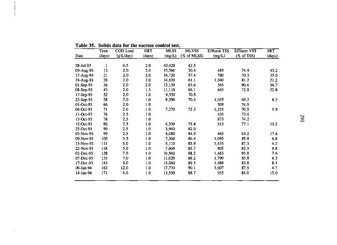
Table 35. Solids data for the sucrose control test. Time COD Load HRT MLSS MLVSS Effluent TSS Effluent VSS SRT
Date (days) (g/L/day) (days) (mg/L) (% of MLSS) (mg/L) (% of TSS) (days)
28-Jul-93 1 0.5 2.0 40,420 42.5 09-Aug-93 13 2.0 2.0 15,560 50.4 485 74.9 43.2 17-Aug-93 21 2.0 2.0 16,720 57.4 780 70.3 35.0 24-Aug-93 28 2.0 2.0 14,620 61.1 1,040 81.2 21.2 Ol-Sep-93 36 2.0 2.0 13,130 63.6 565 80.6 36.7 08-Sep-93 43 2.0 1.5 11.110 66.1 663 72.8 22.8 17-Sep-93 52 2.0 1.0 9,330 70.8 23-Sep-93 58 2.0 1.0 8,590 70.5 1,055 69.2 8.3 Ol-Oct-93 66 2.0 1.0 508 74.9 06-Oct-93 71 2.0 1.0 7,270 72.3 1,255 70.5 5.9 ll-Oct-93 76 2.5 1.0 435 73.6 13-Oct-93 78 2.5 1.0 873 74.2 15-Oct-93 80 2.5 1.0 6,530 75.8 613 77.1 10.5 25-Oct-93 90 2.5 1.0 3,940 82.0 03-NOV-93 99 2.5 1.0 6,080 84.9 465 63.2 17.6 09-NOV-93 105 3.5 1.0 7,360 86.4 1,095 85.8 6.8 15-NOV-93 111 5.0 1.0 6,110 85.9 1,435 87.3 4.2 22-N0V-93 118 5.0 1.0 7,600 85.7 805 82.3 9.8 02-Dec-93 128 7.0 1.0 10,840 88.2 1,463 85.8 7.6 07-Dec-93 133 7.0 1.0 11,020 88.2 1,790 85.8 6.3 17-Dec-93 143 9.0 1.0 15,060 89.5 1,988 83.8 8.1 06-Jan-94 163 12.0 1.0 17,770 90.1 3,907 87.9 4.7 14-Jan-94 171 6.0 1.0 13,550 88.7 955 84.0 15.0

Table 36. COD data for the sucrose+PAC test. Time from Influent COD Effluent TCOD Effluent SCOD
Start-Up HRT COD Load TCOD Removal SCOD Removal
Date (days) (days) (mg/L) (g/L/day) (mg/L) (%) (g/L/day) (%)
26-Jan-93 10 2.00 2,000 1.0 794 60.3 549 72.6
Ol-Feb-93 16 2.00 2,000 1.0 613 69.4 545 72.8
09-Feb-93 24 2.00 2,000 1.0 585 70.8 516 74.2
20-Feb-93 35 4.00 8,000 2.0 1,844 77.0 1,145 85.7
26-Feb-93 41 2.00 4,000 2.0 1,196 70.1 606 84.9
05-Mar-93 48 1.00 2,000 2.0 618 69.1 184 90.8
09-Mar-93 52 1.00 2,000 2.0 650 67.5 182 90.9
19-Mar-93 62 1.00 2,500 2.5 839 66.4 513 79.5
27-Mar-93 70 1.00 3,000 3.0 1,462 51.3 936 68.8
05-Apr-93 79 1.00 3,000 3.0 1,343 55.2 865 71.2
19-Apr-93 93 1.00 4,000 4.0 2,022 49.5 1,187 70.3
28-Apr-93 102 1.00 4,000 4.0 1,804 54.9 1,208 69.8
05-May-93 109 0.75 3,000 4.0 1,549 48.4 885 70.5
ll-May-93 115 0.75 4,000 5.3 2,250 43.8 1,418 64.6
19-May-93 123 0.75 4,000 5.3 1,130 71.8 451 88.7
27-May-93 131 0.75 5,500 7.3 1,174 78.7 380 93.1
02-Jun-93 137 0.75 6,750 9.0 1,362 79.8 184 97.3
14-Jun-93 149 0.75 8,250 11.0 2,280 72.4 240 97.1
21-Jun-93 156 0.75 10,500 14.0 3,129 70.2 263 97.5
30-Jun-93 165 0.75 10,500 14.0 2,036 80.6 401 96.2
15-Jul-93 180 1.00 3,600 3.6 4,769 0.0 3,600 0.0
28-Jul-93 193 2.00 3,538 1.8 1,905 46.2 1,595 54.9
09-Aug-93 205 1.00 3,500 3.5 1,783 49.1 968 72.3

Table 36. (continued). Time from Influent COD Effluent TCOD Effluent SCOD
Start-Up HRT COD Load TCOD Removal SCOD Removal
Date (days) (days) (mg/L) (g/L/day) (mg/L) (%) (g/L/day) (%)
17-Aug-93 213 1.00 3,500 3.5 1,151 67.1 417 88.1
24-Aug-93 220 1.00 5,000 5.0 917 81.7 352 93.0
Ol-Sep-93 228 1.00 7,000 7.0 1,025 85.4 236 96.6
08-Sep-93 235 1.00 9,000 9.0 2,330 74.1 528 94.1
28-Sep-93 255 1.00 12,000 12.0 5,193 56.7 2,958 75.4
06-Oct-93 263 1.00 9,000 9.0 4,349 51.7 3,165 64.8
15-Oct-93 272 1.00 7,000 7.0 2,695 61.5 1,370 80.4

296
Table 37. Biogas data for the sucrose+PAC test. Nominal Std. Methane
HRT COD Load Methane Production Date Day (days) (g/L/day) (% of total) (L/L/day)
16-Jan-93 0 2.00 0.5 17-Jan-93 1 2.00 0.5 66.36 0.03 18-Jan-93 2 2.00 0.5 66.36 0.02 19-Jan-93 3 2.00 0.5 66.36 0.05 20-Jan-93 4 2.00 0.5 66.36 0.05 21-Jan-93 5 2.00 1.0 66.36 0.07 22-Jan-93 6 2.00 1.0 66.36 0.11 23-Jan-93 7 2.00 1.0 66.36 0.15 24-Jan-93 8 2.00 1.0 64.43 0.08 25-Jan-93 9 2.00 1.0 62.49 0.16 26-Jan-93 10 2.00 1.0 62.72 0.14 27-Jan-93 11 2.00 1.0 62.95 0.08 28-Jan-93 12 2.00 1.0 63.18 0.06 29-Jan-93 13 2.00 1.0 62.97 0.09 30-Jan-93 14 2.00 1.0 62.75 0.13 31-Jan-93 15 2.00 1.0 62.54 0.12 Ol-Feb-93 16 2.00 1.0 62.32 0.10 02-Feb-93 17 2.00 1.0 63.33 0.14 03-Feb-93 18 2.00 1.0 64.34 0.15 04-Feb-93 19 2.00 1.0 65.35 0.10 04-Feb-93 19 2.00 1.0 66.35 0.12 05-Feb-93 20 2.00 1.0 67.36 0.16 06-Feb-93 21 2.00 1.0 68.37 0.17 07-Feb-93 22 2.00 1.0 67.16 0.18 08-Feb-93 23 2.00 1.0 65.95 0.11 09-Feb-93 24 2.00 1.0 64.74 0.09 lO-Feb-93 25 2.00 2.0 63.53 0.16 ll-Feb-93 26 2.00 2.0 62.32 0.22 12-Feb-93 27 2.00 2.0 61.11 0.27 13-Feb-93 28 2.00 2.0 59.99 0.27 14-Feb-93 29 4.00 2.0 58.87 0.28 15-Feb-93 30 2.00 2.0 57.75 0.32 16-Feb-93 31 4.00 2.0 57.20 0.28 17-Feb-93 32 4.00 2.0 56.64 0.33 18-Feb-93 33 4.00 2.0 56.09 0.34 19-Feb-93 34 4.00 2.0 55.54 0.42 20-Feb-93 35 4.00 2.0 54.98 0.39 21-Feb-93 36 4,00 2.0 54.43 0.50 22-Feb-93 37 2.00 2.0 55.36 0.45 23-Feb-93 38 2.00 2.0 56.30 0.37 24-Feb-93 39 2.00 2.0 57.23 0.31 25-Feb-93 40 2.00 2.0 58.19 0.35 26-Feb-93 41 2.00 2.0 59.15 0.37 27-Feb-93 42 2.00 2.0 60.10 0.43 28-Feb-93 43 1.50 2.0 61.06 0.43

I .2 ^
S -g -J « 2 J 3 a,'-' in
u ca i 2 •S <5-u o s
TS V 9 C
*-S e e u
I-0) 2 n H
§ ^ a: -p^
tn Tt CN rf
cn On VO CO trj •T)
rf en •*t
Tf "*i-
<N 00 CO in U-) 00 rr CO in 00 00 Tf 0 m 0 «o 0 CO (N in
Tf rj-rj- ON
tT r-Tj- 00 0 «n s On «n «n r-«n s 0 VO 0 in Tf m 00 in m «n Cv m 0 0 d d d d d d d d d d d d d d d d d d d d d d d d d d d d d d d d d d d d d d d d d d
cN O vO m O o *0 — r- cn 00 p in r-p •n fO cs fO VO vd NO i> VO •n VO s CO VO CO VO CO VO <N VO
o o r ^ m - ^ o o r t — « o o r - t n • ^ o ^ i n c n c N v o o N v o f n S fO 0 «n (N VO in Ov CO (S <N
in p 00 00 s 0 (N vO CO
CO CO
Cv r-CO m CO in 00 «n r^' m r-^ •n m o\ m 3 CO VO VO Ov in r--* «n Tf m in CO in r4 in «n d «n «n ci m CO m
o p p p p o o p o « ^ u - i i o i n « / ^ i n i n t n i n p p o p p o p p o p p p o p p p o o p p o p p p o o p c « i r > i r 4 r ^ c > i r > i r > i r 4 r 4 c 4 r 4 r ^ r ^ r 4 r 4 ? S f S r > i f ^ r n r n r n m c n c n f n r n c ^ f n f O t ^ r n f < S r n c < ^ ^ ' ^ T i - T t T f T ) * T i - T t ' ^ ' ^
o o 8 S S S S S S S 8 8 S S S S 8 S S S S 8 8 8 S 8 S S S S S S S 8 8 S S S S S S 8 S S 8
T f t r ) \ o t ^ o o o - - r j m ' « ^ * n \ o r - o o a N ^ cN m vO vo vo 3i o v o r ^ o o a N O ^ c N r * > ^ « o ^ o r - » o o a N O ^ c N c n r f m v o r - o o a N v o v o v o v o v o r ^ r - r ^ - r ^ r ^ r - t ^ r - t ^ r - o o o o o o o o o o o o o o o o o o o o
CO OS CO CN CO CPv CO ON CO On CO On CO On CO On CO On CO Ov CO On CO On CO ON CO On CO On CO CO On CO On CO On CO On CO On CO On CO On CO as CO Ov CO On CO 0\ CO On CO On CO Ov
u« CQ s s s
n s
hN 03 S
u CQ S
c5 s
u. CQ s
(M CQ s
»-• CQ S
(3 s
s s
A s
u CQ s
e3 s
Ui CQ s
tl* cs s 2 s
u* c« S
i-i C3 S
u CO S
u CO S
u c« S
t-> eQ s
Ui CQ s
h« CQ s
s s
0 cs 0
CO 0 s *n
0 c-^ 0
00 0
On 0 0 CO *n NO 00 ck •-iH d (S rJ cs (N CO <s (N <N <N 00 (N (N d CO CO
CO ON CO CO ON
CO ON CO ON
CO ON CO as
CO ON CO ON CO ON CO ON
CO CO ON CO ON CO 0\
t-i Cu
Ui 0. Ui O. a. ii 0. u 0. u* D. IM 0.
UI 0.
UN Q. U> CX IM 0.
li 0. t-i 0. KN Q.
0 0 0 0 0 0 0 0 — TJ- <rv

Table 37. (continued). Nominal Std. Methant
HRT COD Lxjad Methane Production Date Day (days) (g/L/day) (% of total) (L/L/day)
16-Apr-93 90 1.00 4.0 54.61 0.64 17-Apr-93 91 1.00 4.0 55.19 0.63 18-Apr-93 92 1.00 4.0 55.77 0.62 19-Apr-93 93 1.00 4.0 56.35 0.69 20-Apr-93 94 1.00 4.0 56.93 0.73 21-Apr-93 95 1.00 4.0 57.51 0.73 22-Apr-93 96 1.00 4.0 58.09 0.48 23-Apr-93 97 1.00 4.0 58.67 0.22 24-Apr-93 98 1.00 4.0 59.25 0.21 25-Apr-93 99 1.00 4.0 59.83 0.51 26-Apr-93 100 1.00 4.0 60.41 0.60 27-Apr-93 101 1.00 4.0 60.99 0.78 28-Apr-93 102 1.00 4.0 61.57 0.65 29-Apr-93 103 1.00 4.0 61.28 0.70 30-Apr-93 104 1.00 4.0 60.99 0.65 Ol-May-93 105 1.00 4.0 60.69 0.63 02-May-93 106 1.00 4.0 60.40 0.56 03-May-93 107 1.00 4.0 60.11 0.62 04-May-93 108 1.00 4.0 59.53 0.52 05-May-93 109 0.75 5.3 58.96 0.60 06-May-93 110 0.75 5.3 58.38 0.62 07-May-93 111 0.75 5.3 57.80 0.68 08-May-93 112 0.75 5.3 57.22 0.70 09-May-93 113 0.75 5.3 56.65 0.62 lO-May-93 114 0.75 5.3 56.54 0.77 ll-May-93 115 0.75 5.3 56.43 0.63 12-May-93 116 0.75 5.3 56.33 0.65 13-May-93 117 0.75 5.3 56.22 0.74 14-May-93 118 0.75 5.3 56.12 0.81 15-May-93 119 0.75 5.3 56.46 0.85 16-May-93 120 0.75 5.3 56.80 0.84 17-May-93 121 0.75 5.3 57.15 0.90 18-May-93 122 0.75 5.3 57.49 1.01 19-May-93 123 0.75 5.3 57.83 1.05 20-May-93 124 0.75 7.0 58.18 1.25 21-May-93 125 0.75 7.0 58.52 1.52 22-May-93 126 0.75 7.0 58.86 1.56 23-May-93 127 0.75 7.0 59.21 1.57 24-May-93 128 0.75 7.0 59.17 1.57 25-May-93 129 0.75 7.0 59.13 1.68 26-May-93 130 0,75 7.0 59.09 1.62 27-May-93 131 0.75 7.0 59.24 1.80 28-May-93 132 0.75 9.0 59.38 2.06 29-May-93 133 0.75 9.0 59.52 2.30 30-May-93 134 0.75 9.0 59.67 2.28

2 £ in
ON On (N
-a u s
e u
s CQ H
«J -§ § •§ 5 u
CB •o
u n) § 2 •S <»-u o
*0 _ CQ
i z O z u
§ « 53 T3_,
*r> ro
r-(N
U-) en
rj-in
ON r-«n m NO <N
vO 00
»n <s
r-q
00 00 s
O 00
»n ON
00 ON
ON fn
CN NO
ON 00 ON q
fS 00 8
•—H cn
«n ON o TT
ON q
fS ON ON
O ON 00
ON NO
FO 00 o vO
O in RS TS R4 R4 R4 RI RI cs cn en cn C<I ri r4 fS ri rn rn ro cn TT en r4 cn cn rn rn r4 (N (N
Tf ON «r> 00 r-r-^ NO o d d d d
—' >n ON OO ON ON o 00 <N en
NO
s s s s s
On 00 «s rf m On r- 8 m «n NO q On ID VO Tj; NO q <N q cn m 3 *o On vO cs r-->n 00 00 ON o tn o 00 *n NO o in m r-in On r-; q CM (N Tt NO NO 00 00 o fo m «n m 00 Tf
ON »n ON m oo' »n 00 iTi 00 m r-* *r> NO* m NO *n uS ir> *n tn Tj* •n iri «n •Ti to NO »n NO *n \d in to m «r> vd •o in »n •n CO in <N m <N m in d m On Tf 00 Tf 00 NO TT in Tf ON in
q q q q o o q p q o q o q q q q o o q q q p p p q q q q q q o o o p q p q q q o o p q o q O N O N O N O N O N O N O N ' - ^ ^ ^ ' —
*n r- m r- «n in r- tn r-- m «n r- in in t m r-- m r- •n r- in r- m r- in t-- m r-- m in r- •n r- in r- in r- in r- in c in r-- m r «n r- in r- m r-; *n m r- m r- m p-- in r- in r- »n r- in *n r- 8 8 8 8 8 8 8 8 d d d d d d d d d d d d d d d d d d d d d d d d d d d d d d d d d d d d d — ,-4 —- —• —•
i n v o r - o o o N O — ' C N c o T i - m v o r - o o a N O ^ c N f ^ T f i o v o r ^ o o c ^ O ' ^ c s m ' ^ t n v o r - o o O N c n c n f n c n m T f T t ' * ^ T f ' * ^ T t T t ' « ^ - ' ^ T r « n * n » n i n t n t n * n i o ' n « n ' O N O v o v O N O v o s o v o v O N O
m ON
I
CQ
O - ^ C N i m T t w - i v o r - o o o N r ^ r - - r - r - ' r - r - r - - r ^ r - - r - -
ro
cn en m cn en cn en m cn cn fO en fn m m m m en cn c<i m On en On m On m On cn On m On CO On m On ON m ON On m On On CO On On 1 On On On On On On On On OS q\ On On On as CP\ On On o\ On ON ON On On On ON On
1 On
1 On On en On m On m On cn On m On CO On m On ON m ON On m On On CO On
G c c q c q c q q q q q f" q q q q q q q q q q q p q q q q 1 1 1 1 1 1 1 1 1 1 3 3 3 3 3 3 3 3 3 3 3 3 3 3 3 3 3 3 3 3 3 3 3 3 3 3 3 3 3 *3 *3 3 3 3 3 3 3 3 3 3 3 3
«—» •—i »—* *—) —i •—J V •—» »—» «—J "—J —t T •--» •~j •—) •—>
en Tj- »n NO 00 CTN o cn in NO 00 ON O (N Tf «n NO 00 ON O (N fn s
«n VO 00 ON o (N m O O O o o o o O O CN (N (N cs cs (N <N CS cn O O O s o O o o O

Table 37. (continued). Nominal Std. Methant
HRT COD Load Methane Production Date Day (days) (g/L/day) (% of total) (L/L/day)
15-Jul-93 180 1.00 2.0 59.31 0.26 16-Jul-93 181 1.00 2.0 59.15 0.03 17-Jul-93 182 1.00 2.0 58.98 0.00 18-Jul-93 183 1.00 2.0 58.82 0.00 19-Jul-93 184 1.00 2.0 58.65 0.00 20-Jul-93 185 1.00 2.0 58.49 0.00 21-Jul-93 186 1.00 2.0 58.32 0.00 22-Jul-93 187 1.00 2.0 58.16 0.00 23-Jul-93 188 1.00 2.0 57.99 0.29 24-Jul-93 189 1.00 2.0 57.83 0.24 25-Jul-93 190 1.00 2.0 57.66 0.38 26-Jul-93 191 1.00 2.0 57.50 0.67 27-Jul-93 192 1.00 3.5 56.95 0.50 28-Jul-93 193 1.00 3.5 56.40 0.45 29-Jul-93 194 1.00 3.5 55.86 0.41 30-Jul-93 195 1.00 3.5 55.31 0.45 31-Jul-93 196 1.00 3.5 54.76 0.47 Ol-Aug-93 197 1.00 3.5 54.21 0.44 02-Aug-93 198 1.00 3.5 53.66 0.39 03-Aug-93 199 1.00 3.5 54.77 0.58 04-Aug-93 200 1.00 3.5 55.87 0.49 05-Aug-93 201 1.00 3.5 56.97 0.62 06-Aug-93 202 1.00 3.5 58.08 0.64 07-Aug-93 203 1.00 3.5 58.71 0.71 08-Aug-93 204 1.00 3.5 59.34 0.69 09-Aug-93 205 1.00 3.5 59.98 0.72 lO-Aug-93 206 1.00 3.5 60.61 0.80 ll-Aug-93 207 1.00 3.5 61.24 0.80 12-Aug-93 208 1.00 3.5 61.18 0.46 13-Aug-93 209 1.00 3.5 61.12 0.81 14-Aug-93 210 1.00 3.5 61.06 0.83 15-Aug-93 211 1.00 3.5 61.00 0.85 16-Aug-93 212 1.00 3.5 60.94 0.67 17-Aug-93 213 1.00 3.5 60.87 0.93 18-Aug-93 214 1.00 3.5 60.81 0.95 19-Aug-93 215 1.00 5.0 60.75 1.17 20-Aug-93 216 1.00 5.0 60.69 1.30 21-Aug-93 217 1.00 5.0 60.63 1.19 22-Aug-93 218 1.00 5.0 60.57 1.38 23-Aug-93 219 1.00 5.0 60.51 1.48 24-Aug-93 220 1.00 5.0 59.38 1.39 25-Aug-93 221 1.00 7.0 58.25 1.78 26-Aug-93 222 1.00 7.0 57.12 2.10 27-Aug-93 223 1.00 7.0 58.10 2.20 28-Aug-93 224 1.00 7.0 57.71 2.29

301
Table 37. (continued). Nominal Std. Methane
HRT COD Load Methane Production Date Day (days) (g/L/day) (% of total) (L/L/day)
29-Aug-93 225 1.00 7.0 57.32 1.74 30-Aug-93 226 1.00 7.0 56.93 2.24 31-Aug-93 227 1.00 7.0 56.55 2.07 Ol-Sep-93 228 1.00 7.0 56.44 2.03 02-Sep-93 229 1.00 7.0 56.33 0.71 03-Sep-93 230 1.00 7.0 56.22 1.03 04-Sep-93 231 1.00 9.0 56.11 1.40 05-Sep-93 232 1.00 9.0 56.00 1.99 06-Sep-93 233 1.00 9.0 55.89 2.16 07-Sep-93 234 1.00 9.0 55.78 2.32 08-Sep-93 235 1.00 9.0 55.67 2.53 09-Sep-93 236 1.00 9.0 55.57 2.52 lO-Sep-93 237 1.00 9.0 55.89 2.62 ll-Sep-93 238 1.00 9.0 56.21 1.80 12-Sep-93 239 1.00 9.0 56.53 2.04 13-Sep-93 240 1.00 9.0 56.85 2.24 14-Sep-93 241 1.00 12.0 57.17 3.05 15-Sep-93 242 1.00 12.0 57.49 3.53 16-Sep-93 243 1.00 12.0 56.56 4.46 17-Sep-93 244 1.00 12.0 55.62 3.73 18-Sep-93 245 1.00 12.0 54.68 3.56 19-Sep-93 246 1.00 12.0 53.74 3.34 20-Sep-93 247 1.00 12.0 52.81 3.31 21-Sep-93 248 1.00 12.0 51.87 3.39 22-Sep-93 249 1.00 12.0 50.93 4.47 23-Sep-93 250 1.00 12.0 49.99 3.11 24-Sep-93 251 1.00 12.0 49.06 2.10 25-Sep-93 252 1.00 12.0 48.12 2.95 26-Sep-93 253 1.00 12.0 47.18 2.86 27-Sep-93 254 1.00 12.0 46.24 2.60 28-Sep-93 255 1.00 12.0 45.31 2.31 29-Sep-93 256 1.00 9.0 46.39 2.18 30-Sep-93 257 1.00 9.0 47.47 1.81 Ol-Oct-93 258 1.00 9.0 47.53 1.75 02-Oct-93 259 1.00 9.0 47.60 1.60 03-Oct-93 260 1.00 9.0 47.67 1.63 04-Oct-93 261 1.00 9.0 47.73 1.50 05-Oct-93 262 1.00 9.0 47.80 1.21 06-Oct-93 263 1.00 9.0 48.78 0.96 07-Oct-93 264 1.00 7.0 49.77 1.16 08-Oct-93 265 1.00 7.0 50.75 1.07 09-Oct-93 266 1.00 7.0 51.73 1.00 lO-Oct-93 267 1.00 7.0 52.72 1.33 ll-Oct-93 268 1.00 7.0 53.70 1.30

Table 37. (continued). Nominal Std. Methane
HRT COD Load Methane Production Date Day (days) (g/L/day) (% of total) (L/L/day)
12-Oct-93 269 1.00 7.0 54.69 1.38 13-Oct-93 270 1.00 7.0 55.67 1.46 14-Oct-93 271 1.00 7.0 55.72 0.79 15-Oct-93 272 1.00 7.0 55.78 0.15 16-Oct-93 273 1.00 7.0 55.83 1.27 17-Oct-93 274 1.00 7.0 55.89 1.52 18-Oct-93 275 1.00 7.0 55.94 1.82 19-Oct-93 276 1.00 7.0 55.83 1.67 20-Oct-93 277 1.00 7.0 55.71 1.46 21-Oct-93 278 1.00 7.0 55.59 1.55 22-Oct-93 279 1.00 7.0 55.47 1.64 23-Oct-93 280 1.00 7.0 55.36 1.47 24-Oct-93 281 1.00 7.0 55.24 1.52 25-Oct-93 282 1.00 7.0 55.12 1.59 26-Oct-93 283 1.00 7.0 58.72 1.06 27-Oct-93 284 1.00 7.0 62.32 0.09 28-Oct-93 285 1.00 7.0 62.32 0.53 29-Oct-93 286 1.00 7.0 62.32 0.52 30-Oct-93 287 1.00 7.0 62.32 0.45 31-Oct-93 288 1.00 7.0 62.32 0.31 Ol-Nov-93 289 1.00 7.0 62.32 0.31 O2-N0V-93 290 1.00 7.0 62.32 0.52

Table 38. Volatile acids data for the sucrose+PAC test. Time from Start COD Load Volatile Acids
Date (days) (g/L/day) (mg/L as acetic)
23-Jan-93 7 1.0 246 26-Jan-93 10 1.0 339 02-Feb-93 17 1.0 343 lO-Feb-93 25 1.0 334 24-Feb-93 39 2.0 694 14-Mar-93 57 2.5 343 05-Apr-93 79 4.0 647 12-Apr-93 86 4.0 951 05-May-93 109 4.0 711 19-May-93 123 5.3 420 02-Jun-93 137 9.0 60 14-Jun-93 149 11.0 26 21-Jun-93 156 14.0 77 30-Jun-93 165 14.0 86 15-Jul-93 180 3.5 2,589 28-Jul-93 193 3.5 1,209 Ol-Sep-93 228 7.0 120 08-Sep-93 235 9.0 454 28-Sep-93 255 12.0 2,066 06-Oct-93 263 9.0 2,494

304
Table 39. Particle size analysis for the sucrose+PAC test. Time from COD Average Average
Start-up Load Diameter Diameter Date (days) (g/L/day) (arithmetic, ^m) (geometric,
16-Jan-93 0 0.5 31 150 Ol-Feb-93 16 1.0 34 254 15-Feb-93 30 2.0 32 450 05-Mar-93 48 2.0 43 198 24-Mar-93 67 3.0 45 201 19-Apr-93 93 4.0 104 450 24-May-93 128 7.0 67 1,100 05-Jun-93 140 9.0 242 1,837 28-Jul-93 193 3.5 362 2,300 21-Aug-93 217 5.0 345 1,003 17-Sep-93 244 12.0 229 1,500 26-Oct-93 283 7.0 407 1,550

305
Table 40. Alkalinity and pH data for the sucrose+PAC test. Time COD Load Alkalinity pH
Date (days) (g/L/day) (mg/L as CaC03) (miits)
16-Jan-93 0 0.5 1,250 7.53 19-Jan-93 3 0.5 1,320 7.16 23-Jan-93 7 1.0 1,410 6.67 24-Jan-93 8 1.0 1,450 6.60 25-Jan-93 9 1.0 1,460 6.66 26-Jan-93 10 1.0 1,520 6.83 27-Jan-93 11 1.0 1,570 6.80 28-Jan-93 12 1.0 1,510 7.00 31-Jan-93 15 1.0 1,530 6.74 Ol-Feb-93 16 1.0 1,500 6.71 02-Feb-93 17 1.0 1,460 6.66 08-Feb-93 23 1.0 2,580 6.81 09-Feb-93 24 1.0 1,640 6.76 lO-Feb-93 25 1.0 1,800 6.93 ll-Feb-93 26 2.0 2,140 6.64 15-Feb-93 30 2.0 2,690 6.80 24-Feb-93 39 2.0 2,880 6.88 lO-Mar-93 53 2.5 2,390 6.69 14-Mar-93 57 2.5 2,240 6.86 17-Mar-93 60 2.5 2,300 7.50 18-Mar-93 61 2.5 2,410 7.00 19-Mar-93 62 2.5 2,290 6.69 20-Mar-93 63 3.0 2,250 6.71 21-Mar-93 64 3.0 2,310 6.60 22-Mar-93 65 3.0 2,380 6.75 23-Mar-93 66 3.0 2,430 6.80 27-Mar-93 70 3.0 2,270 6.64 28-Mar-93 71 3.0 2,190 6.73 29-Mar-93 72 3.0 2,150 6.78 30-Mar-93 73 3.0 2,170 6.76 31-Mar-93 74 3.0 2,260 6.75 02-Apr-93 76 3.0 2,200 6.75 03-Apr-93 77 3.0 2,150 6.79 05-Apr-93 79 3.0 2,180 6.70 06-Apr-93 80 4.0 2,060 6.62 07-Apr-93 81 4.0 2,250 6.68 08-Apr-93 82 4.0 2,390 6.70 09-Apr-93 83 4.0 2,580 6.61 13-Apr-93 87 4.0 2,620 6.57 15-Apr-93 89 4.0 2,600 6.70 19-Apr-93 93 4.0 2,590 6.70 20-Apr-93 94 4.0 2,670 6.66 21-Apr-93 95 4.0 2,630 6.69 23-Apr-93 97 4.0 2,640 6.84 24-Apr-93 98 4.0 2,650 6.93 27-Apr-93 101 4.0 2,570 6.88

306
Table 40. (continued). Time COD Load Alkalinity pH
Date (days) (g/L/day) (mg/L as CaC03) (units)
Ol-May-93 105 4.0 2,590 6.80 03-May-93 107 4.0 2,490 6.80 04-May-93 108 4.0 2,540 6.80 05-May-93 109 4.0 2,520 6.85 07-May-93 111 5.3 2,530 6.72 08-May-93 112 5.3 2,580 6.70 17-May-93 121 5.3 2,540 6.82 19-May-93 123 5.3 2,560 6.96 20-May-93 124 7.0 2,790 6.82 23-May-93 127 7.0 2,840 6.85 28-May-93 132 9.0 2,970 6.83 Ol-Jun-93 136 9.0 3,030 6.79 02-Jun-93 137 9.0 3,000 6.96 05-Jun-93 140 9.0 3,040 6.87 08-Jun-93 143 11.0 3,150 6.89 14-Jun-93 149 11.0 3,180 6.82 21-Jun-93 156 14.0 3,140 7.02 23-Jun-93 158 14.0 3,290 6.95 28-Jun-93 163 14.0 3,320 7.00 30-Jun-93 165 14.0 3,300 7.07 02-Jul-93 167 14.0 3,290 6.93 05-Jul-93 170 14.0 3,270 7.00 12-Jul-93 177 14.0 3,300 5.32 15-Jul-93 180 3.5 3,200 6.75 19-Jul-93 184 3.5 2,850 7.18 23-Jul-93 188 3.5 2,670 7.03 26-Jul-93 191 3.5 2,590 6.82 28-Jul-93 193 3.5 2,620 6.74 05-Aug-93 201 3.5 2,620 6.74 23-Aug-93 219 5.0 2,600 6.97 25-Aug-93 221 5.0 2,630 6.95 Ol-Sep-93 228 7.0 2,640 6.89 08-Sep-93 235 9.0 2,700 6.92 14-Sep-93 241 12.0 2,830 6.94 20-Sep-93 247 12.0 2,790 6.98 27-Sep-93 254 12.0 2,900 6.90 29-Sep-93 256 12.0 2,830 6.84 04-Oct-93 261 12.0 2,870 6.51 07-Oct-93 264 12.0 2,750 6.75 ll-Oct-93 268 12.0 2,680 6.70 13-Oct-93 270 12.0 2,700 6.86

Table 41. Solids data for the sucrose+PAC test. Time COD Load HRT MLSS MLVSS Effluent TSS Effluent VSS SRT
Date (days) (g/L/day) (days) (mg/L) (% of MLSS) (mg/L) (% of TSS) (days)
16-Jan-93 0 0.5 2.00 21,453 62.9 23-Jan-93 7 1.0 2.00 7,355 63.0 214 77.5 55.9 26-Jan-93 10 1.0 2.00 6,880 63.9 342 56.8 45.3 Ol-Feb-93 16 1.0 2.00 5,120 67.0 188 46.6 78.3 09-Feb-93 24 1.0 2.00 4,645 72.0 136 54.4 90.4 16-Feb-93 31 2.0 4.00 5,035 74.2 20-Feb-93 35 2.0 4.00 5,745 79.0 1,137 74.5 21.4 26-Feb-93 41 2.0 2.00 4,395 80.2 628 79.2 14.2 05-Mar-93 48 2.0 1.00 4,750 81.5 520 74.8 10.0 09-Mar-93 52 2.0 1.00 4,932 82.8 557 71.8 10.2 19-Mar-93 62 2.5 1.00 5,015 86.4 406 79.8 13.4 24-Mar-93 67 3.0 1.00 6,080 85.3 660 78.1 10.1 30-Mar-93 73 3.0 1.00 6,535 87.0 530 77.9 13.8 05-Apr-93 79 3.0 1.00 6,630 86.7 588 76.2 12.8 12-Apr-93 86 4.0 1.00 8,850 85.4 1,356 82.6 6.7 19-Apr-93 93 4.0 1.00 9,950 83.6 1,090 73.6 10.4 28-Apr-93 102 4.0 1.00 7,940 87.7 756 80.9 11.4 05-May-93 109 5.3 0.75 8,590 88.1 848 82.6 8.1 1 l-May-93 115 5.3 0.75 10,015 88.5 1,063 83.3 7.5 19-May-93 123 5.3 0.75 9,250 88.8 868 83.7 8.5 24-May-93 128 7.0 0.75 11,390 88.0 1,287 80.1 7.3 02-Jun-93 137 9.0 0.75 17,230 90.0 1,415 84.8 9.7 06-Jun-93 141 9.0 0.75 18,740 90.0 14-Jun-93 149 11.0 0.75 22,480 91.2 2,045 83.9 9.0 21-Jun-93 156 14.0 0.75 23,400 91.1 3,443 89.3 5.2 30-Jun-93 165 14.0 0.75 26,020 91.8 1,768 86.9 11.7 15-Jul-93 180 2.0 1.00 18,860 90.5 1,950 87.6 10.0 28-Jul-93 193 3.5 1.00 17,140 91.2 577 77.4 35.0 09-Aug-93 205 3.5 1.00 15,340 89.4 1,070 86.7 14.8

Table 41. (continued). Time COD Load HRT MLSS MLVSS Effluent TSS Effluent VSS SRT
Date (days) (g/L/day) (days) (mg/L) (% ofMLSS) (mg/L) (% of TSS) (days)
17-Aug-93 213 3.5 1.00 14,620 89.9 873 83.2 18.1 24-Aug-93 220 5.0 1.00 15,810 90.8 1,150 75.9 16.4 Ol-Sep-93 228 7.0 1.00 19,150 90.5 1,000 85.7 20.2 08-Sep-93 235 9.0 1.00 22,590 90.8 2,118 84.9 11.4 17-Sep-93 244 12.0 1.00 24,730 91.7 23-Sep-93 250 12.0 1.00 24,780 91.0 2,425 83.7 11.1 06-Oct-93 263 9.0 1.00 26,850 90.1 2,050 84.4 14.0 15-Oct-93 272 7.0 1.00 26,470 89.8 1,785 86.5 15.4 25-Oct-93 282 7.0 1.00 26,975 90.1 31-Oct-93 288 7.0 1.00 25,300 87.8

Table 42. COD data for the sucrose+GAC test. Date Day HRT Influent COD Effluent TCOD Effluent SCOD
(days) COD Load TCOD Removal SCOD Removal (mg/L) (g/L/day) (mg/L) (%) (mg/L) (%)
28-Apr-93 9 2.0 2,000 1 2,101 0.0 638 68.1 05-May-93 16 2.0 2,000 1 1,380 31.0 522 73.9 11-May-93 22 2.0 4,000 2 2,370 40.8 1,140 71.5 19-May-93 30 1.5 3,000 2 1,058 64.7 547 81.8 27-May-93 38 1.0 3,000 3 1,223 59.2 730 75.7 02-Jun-93 44 1.0 4,000 4 2,343 41.4 1,495 62.6 14-Jun-93 56 1.0 4,000 4 2,299 42.5 1,359 66.0 21-Jun-93 63 1.0 4,000 4 1,390 65.3 741 81.5 30-Jun-93 72 1.0 5,500 6 1,360 75.3 490 91.1 15-Jul-93 87 1.0 7,000 7 1,645 76.5 347 95.0 28-Jul-93 100 1.0 9,000 9 3,492 61.2 736 91.8 09-Aug-93 112 1.0 9,000 9 4,031 55.2 2,552 71.6 17-Aug-93 120 2.0 15,800 8 4,063 74.3 2,090 86.8 24-Aug-93 127 2.0 15,000 8 15,000 0.0 4,281 71.5 01-Sep-93 135 2.0 10,000 5 4,375 56.3 2,066 79.3 08-Sep-93 142 2.0 10,000 5 5,033 49.7 1,988 80.1 28-Sep-93 162 2.0 10,000 5 4,015 59.9 2,106 78.9 06-Oct-93 170 2.0 10,000 5 2,553 74.5 1,429 85.7

O O U ) < > i t O N > N > t O N ) N ) K ) t O N > N ) M - ^ ^ » — M - ^ ^ M - ^ ^ O O O O O p O O O U J N J t O N > N ) N ) t O N i t s ) N J N ) N -O V O O O ' - J O N ^ 4 ^ U ) h J ^ O v O O O - ^ O N V i 4 i k . U ) N J — 0 ^ 0 0 - ^ a N U j ^ O J K ) ^ O v O O O ' ^ C \ L / l 4 s » - W N ) N - O v O I I I I t I I I I I I I I I I I I I I I I I I I I I I I I I I I I t I I I I I I I I I I I ^ ^ 2 2 2 2 2 2 2 2 2 2 2 2 2 2 2 2 2 2 2 2 2 2 2 2 2 2 2 2 2 2 2 > > > > > > > > > > > > i ^ i ^ . . • • . . • • > a c i a i l l t f l l l l l t l l « l l l l l . . A . ^ . A . ^ ^ ^ . A . A . ^ ^
^ ^ ^ ^ 4 : k . L » J U > U ) U J U J U i W U J W W N J r O N ) N i h J r O r O N ) N ) N i ^ ^ « — 4 i » . U ) N ) ^ O v O O O - - j a N t - ' i 4 ^ W N > ^ O v O O O - - J a s U j 4 i » ' U ) N ) » — O v O O O - g O N L h 4 J > » U J N ) N - O N O O O ' - J a \ U i N>
^ t O N > t O r O K > t 0 4 ^ 4 ^ 4 ^ j : ^ ^ ^ N ) ^ N ) r O b J N > N d r O N ) t O r O N > N > r O t 0 ^ t O N > K ) M ^ t O N > ^ t O N ) N ) t O N > t O N ) N ) 1 / | 0 0 0 0 * 0 0 0 0 0 0 0 0 0 0 0 * 0 0 0 0 0 0 0 0 * 0 0 0 0 0 0 0 0 0 0 0 0 0 0 0 0 0 0 0 0 0
4 ^ 4 ; k 4 i . ^ ^ U J W W L O W U J U J U J U > U i N J t O N > N > N > N > N J l O N 3 N > N > N ) N > ^ ^ ^ ^ ^ ^ o o o o o o o o o o o o o o o o o o o o o o o o o o o o o o o o o o b b o o o b b b o L f t L f t
Ln Ui Ui Ui LA LA LA LA LA LA LA LA LA LA Ui Ui ON -J 00 vO 00 00 00 )0 )D N) b bo Ln N> LA 00 LO 00 lo 00 a\ -J 00 O N) 4^ ON -J 00 ON LA
s s ON ON o\ a\ ON ON •-- •— N> UJ UJ U) 00 UJ ro bv NJ O ON N)
£ 2 ON to s LA --J LA LA LA LA p
LA L»^ LA p\
LA NO Ov N) ON LA On LA ON LA On LA On LA On LA On LA ON LA On LA U>
2 On 4i^ VO N) 00 NJ O
LA VO LO On
LO ON
UJ 0\ On
U) On
L»J On
UJ ON
L»J ON
UJ ON
o o o o o o o o o o o o o o o o o o o o o o o o o o o o o p o o o o o o p o o o p o o o §U > U i i ^ L f t L n ^ 4 i . L j i > . 4 ^ . ; » 4 ^ L ^ l > J U J W U ) L » j L j l » J U ) W U > U > U ) w i o « — O O Q Q Q Q Q O Q Q O Q O Q Q U ) O O V O l ^ O O O U J ~ J O \ O O U l N > O O V . « U l N J N J - ^ 4 ! ^ N J L f i v O O — O ' — O — V 0 > 0 0 0 0 0 0 ' — O O — O — O O

311
Table 43. (continued). Nominal Std Methane
Time HRT COD Load Methane Production Date (days) (days) (g/L/day) (% of total) (L/L/day)
03-Jun-93 45 1.5 4.0 53.45 0.46 04-Jun-93 46 1.5 4.0 52.53 0.42 05-Jim-93 47 1.0 4.0 51.61 0.72 06-Jun-93 48 1.0 4.0 50.68 0.59 07-Jun-93 49 1.0 4.0 50.92 0.61 08-Jun-93 50 1.0 4.0 51.17 0.64 09-Jun-93 51 1.0 4.0 51.41 0.57 lO-Jun-93 52 1.0 4.0 51.65 0.54 ll-Jun-93 53 1.0 4.0 51.89 0.52 12-Jun-93 54 1.0 4.0 52.13 0.54 13-Jun-93 55 1.0 4.0 52.37 0.48 14-Jun-93 56 1.0 4.0 52.61 0.53 15-Jun-93 57 1.0 4.0 52.85 0.61 16-Jun-93 58 1.0 4.0 54.43 0.60 17-Jun-93 59 1.0 4.0 56.01 0.64 18-Jun-93 60 1.0 4.0 57.59 0.65 19-Jun-93 61 1.0 4.0 59.17 0.66 20-Jun-93 62 1.0 4.0 59.07 0.80 21-Jun-93 63 1.0 4.0 58.97 0.81 22-Jun-93 64 1.0 5.5 58.87 0.98 23-Jun-93 65 1.0 5.5 58.78 1.08 24-Jun-93 66 1.0 5.5 58.68 1.15 25-Jun-93 67 1.0 5.5 58.58 1.12 26-Jun-93 68 1.0 5.5 58.48 1.08 27-Jun-93 69 1.0 5.5 58.38 1.10 28-Jun-93 70 1.0 5.5 58.29 1.10 29-Jun-93 71 1.0 5.5 58.19 1.11 30-Jun-93 72 1.0 5.5 58.85 1.22 Ol-Jul-93 73 1.0 5.5 59.51 1.30 02-JU1-93 74 1.0 5.5 60.17 1.32 03-Jul-93 75 1.0 5.5 59.81 1.36 04-Jul-93 76 1.0 5.5 59.44 1.24 05-Jul-93 77 1.0 5.5 59.08 0.96 06-Jul-93 78 1.0 5.5 58.72 1.00 07-Jul-93 79 1.0 5.5 58.36 0.79 08-Jul-93 80 1.0 7.0 58.00 1.50 09-JU1-93 81 1.0 7.0 57.64 1.98 lO-Jul-93 82 1.0 7.0 57.28 1.77 ll-Jul-93 83 1.0 7.0 56.92 1.85 12-Jul-93 84 1.0 7.0 56.56 1.69 13-Jul-93 85 1.0 7.0 56.20 1.88 14-Jul-93 86 1.0 7.0 59.64 2.15 15-Jul-93 87 1.0 7.0 59.27 1.88 16-Jul-93 88 1.0 7.0 58.91 2.09 17-Jul-93 89 1.0 9.0 58.54 2.23
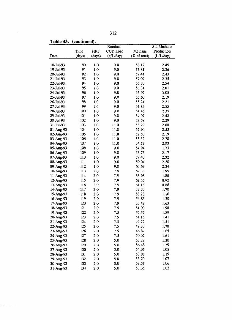
Table 43. (continued). Nominal Std Methan
Time HRT COD Load Methane Production Date (days) (days) (g/L/day) (% of total) (L/L/day)
18-Jul-93 90 1.0 9.0 58.17 2.45 19-Jul-93 91 1.0 9.0 57.81 2.26 20-Jul-93 92 1.0 9.0 57.44 2.43 21-Jul-93 93 1.0 9.0 57.07 2.35 22-Jul-93 94 1.0 9.0 56.70 2.54 23-Jul-93 95 1.0 9.0 56.34 2.01 24-Jul-93 96 1.0 9.0 55.97 3.05 25-Jul-93 97 1.0 9.0 55.60 2.19 26-Jul-93 98 1.0 9.0 55.24 2.21 27-Jul-93 99 1.0 9.0 54.85 2.55 28-Jul-93 100 1.0 9.0 54.46 2.35 29-Jul-93 101 1.0 9.0 54.07 2.42 30-Jul-93 102 1.0 9.0 53.68 2.29 31-Jul-93 103 1.0 11.0 53.29 2.60 Ol-Aug-93 104 1.0 11.0 52.90 2.55 02-Aug-93 105 1.0 11.0 52.50 2.19 03-Aug-93 106 1.0 11.0 53.32 2.78 04-Aug-93 107 1.0 11.0 54.13 2.93 05-Aug-93 108 1.0 9.0 54.94 1.73 06-Aug-93 109 1.0 9.0 55.75 2.17 07-Aug-93 110 1.0 9.0 57.40 2.32 08-Aug-93 111 1.0 9.0 59.04 2.20 09-Aug-93 112 1.0 9.0 60.69 2.34 lO-Aug-93 113 2.0 7.9 62.33 1.95 ll-Aug-93 114 2.0 7.9 63.98 1.80 12-Aug-93 115 2.0 7.9 62.55 0.92 13-Aug-93 116 2.0 7.9 61.13 0.88 14-Aug-93 117 2.0 7.9 59.70 1.70 15-Aug-93 118 2.0 7.9 58.28 1.16 16-Aug-93 119 2.0 7.9 56.85 1.30 17-Aug-93 120 2.0 7.9 55.43 1.63 18-Aug-93 121 2.0 7.5 54.00 1.90 19-Aug-93 122 2.0 7.5 52.57 1.89 20-Aug-93 123 2.0 7.5 51.15 1.41 21-Aug-93 124 2.0 7.5 49.72 1.51 22-Aug-93 125 2.0 7.5 48.30 1.70 23-Aug-93 126 2.0 7.5 46.87 1.65 24-Aug-93 127 2.0 7.5 50.07 1.61 25-Aug-93 128 2.0 5.0 53.28 1.30 26-Aug-93 129 2.0 5.0 56.48 1.29 27-Aug-93 130 2.0 5.0 54.05 1.08 28-Aug-93 131 2.0 5.0 53.88 1.19 29-Aug-93 132 2.0 5.0 53.70 1.07 30-Aug-93 133 2.0 5.0 53.53 1.06 31-Aug-93 134 2.0 5.0 53.35 1.02

313
Table 43. (continued). Nominal Std Methane
Time HRT COD Load Methane Production Date (days) (days) (g/L/day) (% of total) (L/L/day)
Ol-Sep-93 135 2.0 5.0 53.49 1.11 02-Sep-93 136 2.0 5.0 53.63 0.42 03-Sep-93 137 2.0 5.0 53.77 0.47 ()4-Sep-93 138 2.0 5.0 53.91 0.86 05-Sep-93 139 2.0 5.0 54.05 1.11 06-Sep-93 140 2.0 5.0 54.19 0.94 07-Sep-93 141 2.0 5.0 54.33 0.88 08-Sep-93 142 2.0 5.0 54.47 1.17 09-Sep-93 143 2.0 5.0 54.61 1.35 lO-Sep-93 144 2.0 5.0 55.04 1.17 ll-Sep-93 145 4.0 5.0 55.47 1.17 12-Sep-93 146 4.0 5.0 55.90 1.41 13-Sep-93 147 4.0 5.0 56.33 1.49 14-Sep-93 148 4.0 5.0 56.76 1.26 15-Sep-93 149 4.0 5.0 57.19 0.86 16-Sep-93 150 4.0 5.0 56.86 1.27 17-Sep-93 151 4.0 5.0 56.53 1.55 18-Sep-93 152 4.0 5.0 56.21 1.34 19-Sep-93 153 4.0 5.0 55.88 1.40 20-Sep-93 154 4.0 5.0 55.55 1.30 21-Sep-93 155 4.0 5.0 55.23 1.38 22-Sep-93 156 2.0 5.0 54.90 1.10 23-Sep-93 157 2.0 5.0 54.57 0.97 24-Sep-93 158 2.0 5.0 54.25 1.09 25-Sep-93 159 2.0 5.0 53.92 0.93 26-Sep-93 160 2.0 5.0 53.59 1.02 27-Sep-93 161 2.0 5.0 53.27 0.90 28-Sep-93 162 2.0 5.0 52.94 1.09 29-Sep-93 163 2.0 5.0 53.54 1.06 30-Sep-93 164 2.0 5.0 54.13 0.99 Ol-Oct-93 165 2.0 5.0 54.49 1.00 02-Oct-93 166 2.0 5.0 54.86 1.17 03-Oct-93 167 2.0 5.0 55.22 1.20 04-Oct-93 168 2.0 5.0 55.59 1.08 05-Oct-93 169 2.0 5.0 55.95 1.06 06-Oct-93 170 2.0 5.0 55.64 1.01 07-Oct-93 171 2.0 5.0 55.33 0.99 08-Oct-93 172 2.0 5.0 55.02 0.97 09-Oct-93 173 2.0 5.0 54.71 0.98 lO-Oct-93 174 2.0 5.0 54.40 0.98 ll-Oct-93 175 2.0 5.0 54.09 0.95 12-Oct-93 176 2.0 5.0 53.78 1.06 13-Oct-93 177 2.0 5.0 53.47 0.99 14-Oct-93 178 2.0 5.0 54.37 1.05 15-Oct-93 179 2.0 5.0 55.27 1.11

314
Table 43. (continued). Nominal Std Methane
Time HRT COD Load Methane Production Date (days) (days) (g/L/day) (% of total) (L/L/day)
16-Oct-93 180 2.0 5.0 56.17 1.22 I7-Oct-93 181 2.0 5.0 57.08 1.27 18-Oct-93 182 2.0 5.0 57.98 1.25 19-Oct-93 183 2.0 5.0 57.96 1.39 20-Oct-93 184 2.0 5.0 57.95 1.30 21-Oct-93 185 2.0 5.0 57.94 1.19 22-Oct-93 186 2.0 5.0 57.92 1.30 23-Oct-93 187 2.0 5.0 57.91 1.21 24-Oct-93 188 2.0 5.0 57.89 1.20 25-Oct-93 189 2.0 5.0 57.88 1.18 26-Oct-93 190 2.0 5.0 60.68 0.62 27-Oct-93 191 2.0 5.0 63.47 0.13 28-Oct-93 192 2.0 5.0 63.47 0.29 29-Oct-93 193 2.0 5.0 63.47 0.35 30-Oct-93 194 2.0 5.0 63.47 0.74 31-Oct-93 195 2.0 5.0 63.47 0.20 Ol-Nov-93 196 2,0 5.0 63.47 0.18 O2-N0V-93 197 2.0 5.0 63.47 0.61

315
Table 44. Volatile acids data for the sucrose+GAC test.
Date Time from Start
(days) COD Load (g/L/day)
Volatile Acids (mg/L as acetic)
05-May-93 16 1.0 369 19-May-93 30 2.0 420 02-Jun-93 44 4.0 1,054 14-Jun-93 56 4.0 1,046 21-Jun-93 63 4.0 523 30-Jun-93 72 5.5 223 15-Jul-93 87 7.0 60 28-Jul-93 100 9.0 50 Ol-Sep-93 135 5.0 1,380 08-Sep-93 142 5.0 1,397 28-Sep-93 162 5.0 1,414 06-Oct-93 170 5.0 1,106
Table 45. Particle size analysis for the sucrose+GAC test. Time from COD Average Average
Start-up Load Diameter Diameter Date (days) (g/L/day) (arithmetic, /im) (geometric, fxt
19-Apr-93 0 1.0 89 300 24-May-93 35 3.0 38 400 05-Jun-93 47 4.0 35 500 28-Jul-93 100 9.0 74 All 26-Aug-93 129 5.0 405 1,174 17-Sep-93 151 5.0 250 1,899 26-Oct-93 190 5.0 150 1,166

316
Table 46. Alkalinity and pH data for the sucrose+GAC test. Time COD Load Alkalinity pH
Date (days) (g/L/day) (mg/L as CaC03) (units)
20-Apr-93 1 0.5 2,580 7.13 21-Apr-93 2 1.0 2,550 7.09 23-Apr-93 4 1.0 2,600 7.30 24-Apr-93 5 1.0 2,590 7.14 27-Apr-93 8 1.0 2,680 6.96 Ol-May-93 12 1.0 2,680 6.91 03-May-93 14 1.0 2,670 7.07 04-May-93 15 1.0 2,700 7.25 05-May-93 16 1.0 2,720 7.27 07-May-93 18 2.0 2,800 6.84 08-May-93 19 2.0 2,970 6.75 17-May-93 28 2.0 3,050 6.95 19-May-93 30 2.0 3,060 7.11 20-May-93 31 3.0 3,030 6.85 23-May-93 34 3.0 2,890 6.74 28-May-93 39 3.0 2,870 6.81 Ol-Jun-93 43 4.0 2,750 6.60 02-Jun-93 44 4.0 2,700 6.76 05-Jun-93 47 4.0 2,690 6.82 08-Jun-93 50 4.0 2,650 6.72 14-Jun-93 56 4.0, 2,750 6.67 21-Jun-93 63 4.0 2,690 6.96 23-Jun-93 65 5.5 2,700 6.68 28-Jun-93 70 5.5 2,860 6.81 30-Jun-93 72 5.5 2,880 7.01 02-Jul-93 74 5.5 2,820 6.92 05-Jul-93 77 5.5 2,800 7.00 12-Jul-93 84 5.5 2,760 6.93 15-Jul-93 87 7.0 2,640 6.96 19-Jul-93 91 9.0 2,600 7.08 23-Jul-93 95 9.0 2,570 7.21 26-Jul-93 98 9.0 2,650 6.94 28-Jul-93 100 9.0 2,640 6.85 05-Aug-93 108 9.0 2,680 6.95 23-Aug-93 126 8.0 2,660 6.76 25-Aug-93 128 5.0 2,750 6.78 Ol-Sep-93 135 5.0 2,770 6.80 08-Sep-93 142 5.0 2,770 6.92 14-Sep-93 148 5.0 2,790 6.99 20-Sep-93 154 5.0 2,780 7.04 27-Sep-93 161 5.0 2,670 6.85 04-Oct-93 168 5.0 2,590 6.85 07-Oct-93 171 5.0 2,650 6.90 ll-Oct-93 175 5.0 2,740 6.72 13-Oct-93 177 5.0 2,800 6.89

Table 47. Solids data for the sucrose+GAC test. Date Day COD Load HRT MLSS MLVSS Effluent TSS Effluent VSS SRT
(g/L/day) (days) (mg/L) (% of MLSS) (mg/L) (% of TSS) (days)
19-Apr-93 0 0.5 2.0 19,000 63.3 28-Apr-93 9 I.O 2.0 9,375 62.0 2,044 61.4 9.3 05-May-93 16 1.0 2.0 8,490 63.3 1,105 62.9 15.5 ll-May-93 22 2.0 2.0 8,570 69.9 1,550 70.6 10.9 19-May-93 30 3.0 1.5 6,390 76.8 754 75.4 12.9 24-May-93 35 3.0 1.0 5,310 75.5 623 75.5 8.5 02-Jun-93 44 4.0 1.0 6,800 82.9 1,080 80.8 6.5 06-Jiin-93 48 4.0 1.0 6,440 83.9 14-Jun-93 56 4.0 1.0 6,980 84.5 1,155 79.2 6.4 21-Jun-93 63 4.0 1.0 8,760 86.2 790 82.9 11.5 30-Jun-93 72 5.5 1.0 12,400 88.0 913 86.1 13.9 15-Jul-93 87 7.0 1.0 17,910 88.8 1,543 88.0 11.7 28-Jul-93 100 9.0 1.0 15,440 90.7 3,037 88.9 5.2 09-Aug-93 112 9.0 1.0 7,400 89.9 1,923 86.7 4.0 17-Aug-93 120 7.9 2.0 9,720 88.7 2,612 88.4 7.5 24-Aug-93 127 7.5 2.0 7,130 89.7 3,005 89.0 4.8 Ol-Sep-93 135 5.0 2.0 5,510 90.5 2,708 89.1 4.1 08-Sep-93 142 5.0 2.0 7,940 87.1 3,695 86.5 4.3 17-Sep-93 151 5.0 4.0 9,970 84.8 23-Sep-93 157 5.0 2.0 7,150 83.5 3,240 87.0 4.2 Ol-Oct-93 165 5.0 2.0 1,118 85.2 06-Oct-93 170 5.0 2.0 10,550 87.5 1,665 84.1 13.2 ll-Oct-93 175 5.0 2.0 425 75.3 13-Oct-93 177 5.0 2.0 2,805 88.7 15-Oct-93 179 5.0 2.0 13,320 83.3 445 74.2 67.2

Table 48. COD data for the sucrose+garnet test. Time from Influent COD Effluent TCOD Effluent SCOD Start-Up HRT COD Load TCOD Removal SCOD Removal
Date (days) (days) (mg/L) (g/L/day) (mg/L) (%) (mg/L) (%)
27-May-93 7 2.0 2,000 1.0 676 66.2 524 73.8 02-Jun-93 13 2.0 4,000 2.0 2,546 36.4 1,687 57.8 14-Jun-93 25 2.0 4,000 2.0 3,324 16.9 828 79.3 21-Jun-93 32 2.0 4,000 2.0 1,603 59.9 737 81.6 30-Jun-93 41 1.5 4,000 2.7 1,419 64.5 1,013 74.7 05-Jul-93 46 1.5 4,000 2.7 1,440 64.0 533 86.7 15-Jul-93 56 1.0 3,500 3.5 2,503 28.5 2,148 38.6 28-Jul-93 69 1.0 3,500 3.5 2,710 22.6 1,928 44.9 09-Aug-93 81 1.0 3,500 3.5 2,164 38.2 1,402 59.9 17-Aug-93 89 1.0 3,500 3.5 2,483 29.1 1,151 67.1 24-Aug-93 96 2.0 7,000 3.5 3,195 54.4 1,880 73.1 Ol-Sep-93 104 2.0 7,000 3.5 3,159 54.9 1,610 77.0 08-Sep-93 111 2.0 7,000 3.5 3,511 49.8 1,616 76.9 28-Sep-93 131 2.0 7,000 3.5 4,468 36.2 2,898 58.6 06-Oct-93 139 2.0 7,000 3.5 2,797 60.0 2,309 67.0

319
Table 49. Biogas data for the sucrose+garnet test. Nomial Std. Methane
Time HRT COD Load Production Date (days) (days) (g/L/day) (L/L/day)
20-May-93 0 2.0 0.5 21-May-93 1 2.0 0.5 0.00 22-May-93 2 2.0 1.0 0.00 23-May-93 3 2.0 1.0 0.21 24-May-93 4 2.0 1.0 0.18 25-May-93 5 2.0 1.0 0.15 26-May-93 6 2.0 1.0 0.13 27-May-93 7 2.0 1.0 0.11 28-May-93 8 2.0 1.0 0.09 29-May-93 9 2.0 2.0 0.14 30-May-93 10 2.0 2.0 0.17 31-May-93 11 2.0 2.0 0.27 Ol-Jun-93 12 2.0 2.0 0.17 02-Jun-93 13 2.0 2.0 0.20 03-Jun-93 14 2.0 2.0 0.15 04-Jun-93 15 2.0 2.0 0.23 05-Jun-93 16 2.0 2.0 0.16 06-Jun-93 17 2.0 2.0 0.17 07-Jun-93 18 2.0 2.0 0.19 08-Jun-93 19 2.0 2.0 0.18 09-Jun-93 20 2.0 2.0 0.22 lO-Jun-93 21 2.0 2.0 0.12 ll-Jun-93 22 2.0 2.0 0.21 12-Jun-93 23 2.0 2.0 0.28 13-Jun-93 24 2.0 2.0 0.26 14-Jun-93 25 2.0 2.0 0.24 15-Jun-93 26 2.0 2.0 0.18 16-Jun-93 27 2.0 2.0 0.32 17-Jun-93 28 2.0 2.0 0.37 18-Jun-93 29 2.0 2.0 0.45 19-Jun-93 30 2.0 2.0 0.39 20-Jun-93 31 2.0 2.0 0.43 21-Jun-93 32 2.0 2.0 0.43 22-Jun-93 33 1.5 2.7 0.47 23-Jun-93 34 1.5 2.7 0.50 24-Jun-93 35 1.5 2.7 0.52 25-Jun-93 36 1.5 2.7 0.45 26-Jun-93 37 1.5 2.7 0.50 27-Jun-93 38 1.5 2.7 0.44 28-Jun-93 39 1.5 2.7 0.40 29-Jun-93 40 1.5 2.7 0.45 30-Jun-93 41 1.5 2.7 0.53 Ol-Jul-93 42 1.5 2.7 0.56 02-Jul-93 43 1.5 2.7 0.58 03-Jul-93 44 1.5 2.7 0.58

«ri •o
in Tj- Ov cn <N cn
vo fs o rs 00 «r>
cn ON r-" ON cn cs
d d d d d d d d d d d d d d (S rj-(N \o <N
vo < s ON CN o cn r-cs
so (N ON <N o cn o cn Tj-cn cn cn
d d d d d d d d d d d d d d
'Tt- —
d d c i d d d d d d d d d d d d
r ^ r ^ r - - r - - ' n u - > » o m v * i m t n « n < o m v ^ « n t n ' n « o v n w i m i o » o m » n « n « r > » n « n m m i n « n » r ) m i r i « n « n i o » n » n < o m « r ) f ^ r ^ r ^ r ^ c n ( ^ r n c < ^ r o c n r n f n f n r n f < ^ r n c O f O f n c n c < i c n r n f n r ^ r n r o r n f ^ r n c n f n c < ^ r n c o c n c ^ c n f * ^ c ^ f ^ r n r ^ f ^ < ^
t n « n « n u - > 0 0 0 0 0 0 0 0 0 0 0 0 0 0 0 0 0 0 0 0 0 0 0 0 0 0 0 0 0 0 0 0 0 0 0 0 0 0 0 0 0
i o v o r - o o O N O ' - ^ t N f n T t w - > v o r - o o o \ • ^ • T 3 - - r f T r T f i n « n m m » n < n » n m « n i n S 3 r ^ m - ^ u ^ v o r - o o O N O ^ c N f ^ T j - m ^ o r - o o O N O v o v o v o v o v o v o v o v o r - r - r - r - t ^ t ^ r - ^ ^ ^ — ^ ^ ^ < s r n T j * m v o r - o o a N
r > - r * » o o o o o o o o o o o o o o o o o o o o
f n m m r ^ c n f n f n m m m m f o m m m r < ^ m c < > m c n f n f n m m ^ o m m m O N O ^ O ^ O ^ C ^ O ^ a ^ o ^ C T \ 0 ^ 0 ^ 0 ^ 0 ^ 0 ^ 0 \ O ^ C ^ ' ^ ' ^ ' = ^ ^ ^ ' = r ^ ' ^ ' = r ^ ^ ? ^ ^ s ^ ^ ^ ^ ^ ? ? ' ^ ? < ? < ? = ^ ' = r ' = 7 ^ ^ w ) t i o d o t 5 o o o o o ( i ) w ) o o t i o w ) o o o o w ) t i o o o o o
I I I I I I I • I I I I • I I I I I I I I I I I I t I I I t I I I I I I I I t t I I ( I I
Si r > v o t ~ o o o \ o — c N m T t < n v o c ~ o o o v o - ^ r ^ c « ^ ' : r > n v o r ~ o o o \ o — < — > f S c « ^ - < 4 - > r i v o t ~ - o o o \ o — ' C M c o T t i n v o r -O O O O O — — — — — ' - ^ t N t S C N f N t N t N f N f S C N C N r ' i m O O O O O O O O O — '

O W t O N ) K > t O N ) K ) M t O r O t O ^ — ^ O v O 0 0 - J O N L n ^ W N J « - - O v O 0 0 ^ 0 s L h ^ U J h J > - * O ^ 0 0 - ^ 0 N ^
O O O W U J t O r O t O t O N > r O K ) N J N > K > H - » — U > N ) H - ^ O v £ > 0 0 - J O N U i - P i . W N > » - O V O O O
n C / 3 C / 3 C / a C / 5 C / 3 C / I C / 3 C / 5 C / 5 C / 5 C / 3 C / 3 C / 3 C / 5 C / 5 C « C / 3 C / 3 C / 3 C / 3 C / 5 C / 5 C / 5 C / 5 C / 3 C / 5 C / 5 C / D C / 5 C / 3 > > > > > > > > > > > > > > > r o f t r D f 6 0 f 6 r D r t f D « Q r t r & r D o n f t r t f D f B O « r t < i f D « « O f D f 5 e e c e e e e e e e c e e e S - a - a ^ ^ ' T 3 - 0 ' 0 - 0 ^ ' T 3 T 3 T 3 - a - a ' a T 3 - a ' a ^ - a ^ ' 0 T p - 0 T 3 ^ - a ' T p - a ' a ( = ( g « ^ ( g ( g j g j g ( g ( g t g t g ( g ( g ^ 0 v 0 v O v 0 s 0 v 0 v 0 ^ 0 > 0 v 0 \ D v O \ 0 > 0 N 0 ' O v 0 v 0 v 0 > 0 v 0 v 0 v 0 ' O v 0 s 0 ^ v 0 N 0 v 0 v 0 y U v i 3 v i 3 N i 3 v i 5 > i 5 \ V v i 3 v n v i 5 s 0 \ C \ r 5 \ i 3 W L » J U ) W W U J U J W U ) L » i O i U ) U ) O J U > W U » U i U J U ) U > ^ > a U ) U J U J O J W U ) W U > U i { g S j g g g J g j g S g J 2 S S { g g
U i U > l > J U i U J N i N 3 N J t s ) K ) t O N J r s i r s ) S ) ^ ^ ^ ^ ^ ' — • — ^ ^ ^ O O O O O O ^ 0 0 * > J 0 N U i - P » - U ) h J H - O ^ 0 0 - - - J O L / l 4 ^ U ) N J ' — O V O O O - J O N U I
O O O O ^ v O v O v O v O v O ^ v O v O v O U > r O K - O v O O O - - J O N L f i 4 ^ U ) N ) — o
N > t O N > r O N ) N ) h J r o r s ) N ) 4 ^ ^ ^ 4 : ^ 4 ^ ^ ^ ^ 4 ^ 4 : ^ - p w b O N ) t O N ) N > N > N ) N ) N > ^ N ) N ) N ; t O r O t O t O N ) N > N ) | s ) N ) N ) H ^ b b b b b b b b b b b b b b b b b b b b b b b b b b b b b b b b b b b b b b b b b b b b b
L a U J L » J L a U > U > U > U J U J L O U > U J U > L ^ ( > ^ U ) U > L » J L O U ) U > U J L O U J U J U ^ U > U J U > U > U ^ U ^ U ) U ^ U > U 3 U J < > ^ U ) U > U > U ^ U > L » J U > l ^ l ^ L h L r » L n U i L n L h L h U > L h l ^ l ^ l ^ L h U j V ^ L r t L n L h l / i L h U i L h L h L r i l ^ l / i L h L r > t ^ L n u » L n L n l / i L / > L n L f > L f t l / i L / » U i L r i * U i
p p p p p p p p p p p a \ a v ^ t o N ) N ) L o 4 ^ L > ^ 4 : k . W W O O ^ O ^ U ^ C T ^ N J W W - J
p p p p p p p p p p p 4:^ 4^ LA .pk. Ln Ln ^ a\ L/i
p p p p p p p p p p p l / i l / i L f t u i L r t b ^ ^ o s L / i L n ^ ^ > 4 4 i ^ 4 i » ' L / » W O W V O ' - J O
p p p p p p p p p p p p O N O N W ^ c ^ C N O N O t L f t L r t L f t L f t w o ^ v o < y » » — • — O O ^ ^ U t O
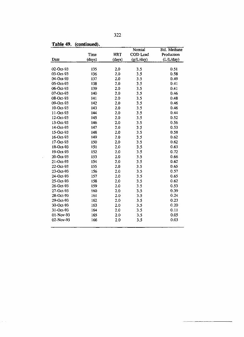
322
Table 49. (continued). Nomial Std. Methane
Time HRT COD Load Production Date (days) (days) (g/L/day) (L/L/day)
02-Oct-93 135 2.0 3.5 0.51 03-Oct-93 136 2.0 3.5 0.58 04-Oct-93 137 2.0 3.5 0.49 05-Oct-93 138 2.0 3.5 0.41 06-Oct-93 139 2.0 3.5 0.41 07-Oct-93 140 2.0 3.5 0.46 08-Oct-93 141 2.0 3.5 0.48 09-Oct-93 142 2.0 3.5 0.46 lO-Oct-93 143 2.0 3.5 0.46 ll-Oct-93 144 2.0 3.5 0.44 12-Oct-93 145 2.0 3.5 0.52 13-Oct-93 146 2.0 3.5 0.56 14-Oct-93 147 2.0 3.5 0.53 15-Oct-93 148 2.0 3.5 0.58 16-Oct-93 149 2.0 3.5 0.62 17-Oct-93 150 2.0 3.5 0.62 18-Oct-93 151 2.0 3.5 0.63 19-Oct-93 152 2.0 3.5 0.72 20-Oct-93 153 2.0 3.5 0.66 21-Oct-93 154 2.0 3.5 0.62 22-Oct-93 155 2.0 3.5 0.65 23-Oct-93 156 2.0 3.5 0.57 24-Oct-93 157 2.0 3.5 0.65 25-Oct-93 158 2.0 3.5 0.62 26-Oct-93 159 2.0 3.5 0.53 27-OCI-93 160 2.0 3.5 0.39 28-Oct-93 161 2.0 3.5 0.24 29-Oct-93 162 2.0 3.5 0.23 30-Oct-93 163 2.0 3.5 0.20 31-Oct-93 164 2.0 3.5 0.11 Ol-Nov-93 165 2.0 3.5 0.05 O2-N0V-93 166 2.0 3.5 0.03

323
Table 50. Volatile acids data for the sucrose+garnet test.
Date Time from Start
(days) COD Load (g/L/day)
Volatile Acids (mg/L as acetic)
02-Jun-93 13 2.0 1,106 14-Jun-93 25 2.0 523 21-Jun-93 32 2.0 489 30'Jun-93 41 2.7 694 15-Jul-93 56 3.5 1,517 28-Jul-93 69 3.5 1,483 Ol-Sep-93 104 3.5 1,320 08-Sep-93 111 3.5 1,286 28-Sep-93 131 3.5 1,963
Table 51. Particle size analysis for the sucrose+garnet test. Time from COD Average Average
Start-up Load Diameter Diameter Date (days) (g/L/day) (arithmetic, ^m) (geometric, /xm)
24-May-93 4 1.0 33 150 28-Jul-93 69 3.5 69 300 26-Aug-93 98 3.5 102 450 17-Sep-93 120 3.5 146 600 26-Oct-93 159 3.5 40 500

324
Table 52. Alkalinity and pH data for the sucrose+garnet test. Time COD Lx)ad Alkalinity pH
Date (days) (g/L/day) (mg/L as CaC03) (units)
23-May-93 1 1.0 2,250 7.08 28-May-93 6 1.0 2,300 6.95 Ol-Jun-93 10 2.0 2,320 6.64 02-Jun-93 11 2.0 2,400 6.71 05-Jun-93 14 2.0 2,540 6.81 08-Jun-93 17 2.0 2,590 6.80 14-Jun-93 23 2.0 2,540 6.76 21-Jun-93 30 2.0 2,640 6.97 23-Jun-93 32 2.7 2,710 6.77 28-Jun-93 37 2.7 2,760 6.84 30-Jun-93 39 2.7 2,800 6.90 02-Jul-93 41 2.7 2,690 7.00 05-Jul-93 44 2.7 2,740 6.89 12-Jul-93 51 3.5 2,830 6.74 15-Jul-93 54 3.5 2,800 6.64 19-Jul-93 58 3.5 2,810 6.82 23-Jul-93 62 3.5 2,650 6.61 26-Jul-93 65 3.5 2,740 6.67 28-Jul-93 67 3.5 2,700 6.64 05-Aug-93 75 3.5 2,730 6.69 23-Aug-93 93 3.5 2,610 6.72 25-Aug-93 95 3.5 2,580 6.75 Ol-Sep-93 102 3.5 2,650 6.79 08-Sep-93 109 3.5 2,600 6.83 14-Sep-93 115 3.5 2,760 6.80 20-Sep-93 121 3.5 2,750 6.77 27-Sep-93 128 3.5 2,630 6.56 29-Sep-93 130 3.5 2,780 7,15 04-Oct-93 135 3.5 2,690 6.60 07-Oct-93 138 3.5 2,700 6.79 1 l-Oct-93 142 3.5 2,820 6.60 13-Oct-93 144 3.5 2,870 6.77
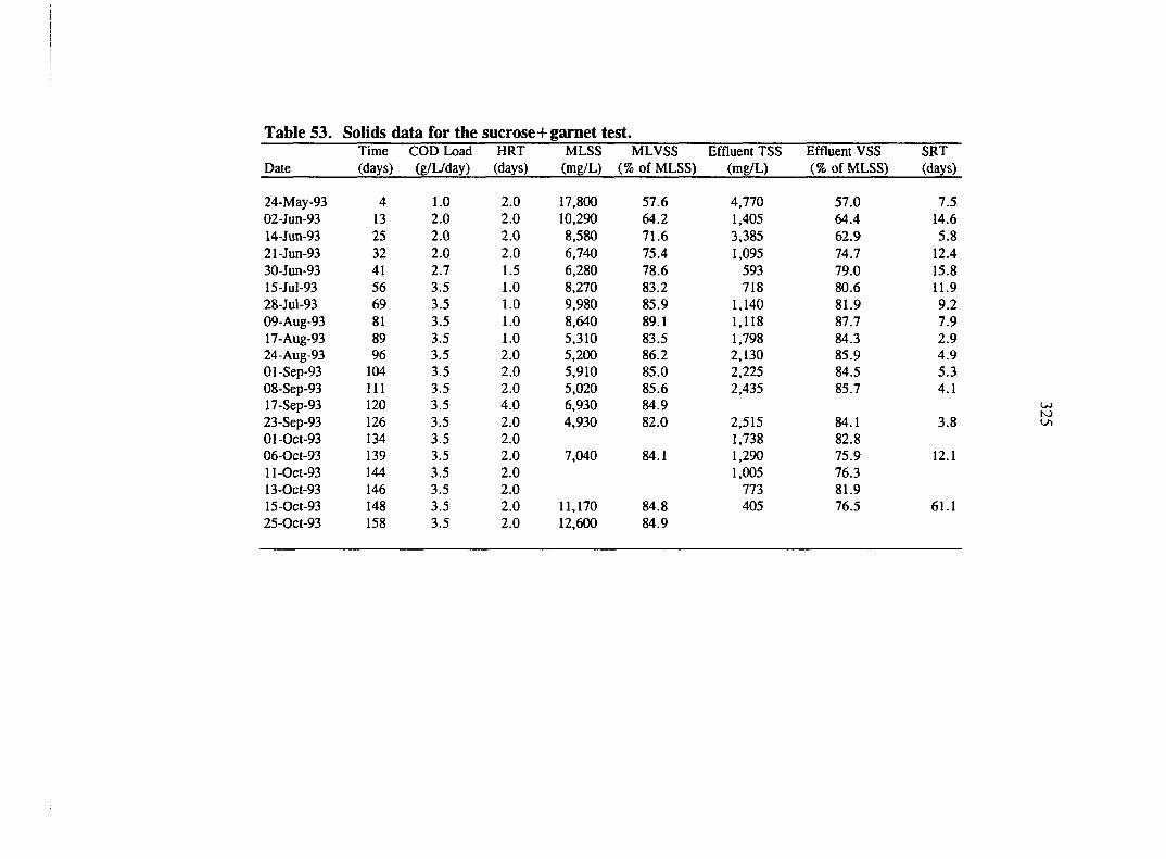
Table 53. Solids data for the sucrose+garnet test. Time COD Load HRT MLSS MLVSS Effluent TSS Effluent VSS SRT
Date (days) (g/L/day) (days) (mg/L) (% of MLSS) (mg/L) (% of MLSS) (days)
24-May-93 4 1.0 2.0 17,800 57.6 4,770 57.0 7.5 02-Jun-93 13 2.0 2.0 10,290 64.2 1,405 64.4 14.6 14-Jun-93 25 2.0 2.0 8,580 71.6 3,385 62.9 5.8 21-Jun-93 32 2.0 2.0 6,740 75.4 1,095 74.7 12.4 30-Jun-93 41 2.7 1.5 6,280 78.6 593 79.0 15.8 15-M-93 56 3.5 1.0 8,270 83.2 718 80.6 11.9 28-Jul-93 69 3.5 1.0 9,980 85.9 1,140 81.9 9.2 09-Aug-93 81 3.5 1.0 8,640 89.1 1,118 87.7 7.9 17-Aug-93 89 3.5 1.0 5,310 83.5 1,798 84.3 2.9 24-Aug-93 96 3.5 2.0 5,200 86.2 2,130 85.9 4.9 Ol-Sep-93 104 3.5 2.0 5,910 85.0 2,225 84.5 5.3 08-Sep-93 111 3.5 2.0 5,020 85.6 2,435 85.7 4.1 17-Sep-93 120 3.5 4.0 6,930 84.9 23-Sep-93 126 3.5 2.0 4,930 82.0 2,515 84.1 3.8 Ol-Oct-93 134 3.5 2.0 1,738 82.8 06-Oct-93 139 3.5 2.0 7,040 84.1 1,290 75.9 12.1 ll-Oct-93 144 3.5 2.0 1,005 76.3 13-Oct-93 146 3.5 2.0 773 81.9 15-Oct-93 148 3.5 2.0 11,170 84.8 405 76.5 61.1 25-Oct-93 158 3.5 2.0 12,600 84.9

Table 54. COD data for the sucrose+sand test. Time from Influent COD Effluent TCOD Effluent SCOD Start-Up HRT COD Load TOCD Removal SCOD Removal
Date (days) (days) (mg/L) (g/L/day) (mg/L) (%) (mg/L) (%)
27-May-93 7 2.0 2,000 1.0 2,131 0.0 744 62.8 02-Jun-93 13 2.0 4,000 2.0 3,129 21.8 1,932 51.7 14-Jun-93 25 2.0 4,000 2.0 1,897 52.6 1,479 63.0 21-Jun-93 32 2.0 4,000 2.0 1,584 60.4 1,124 71.9 30-Jun-93 41 1.5 4,000 2.7 1,494 62.7 1,248 68.8 05-Jul-93 46 1.5 4,000 2.7 2,123 46.9 1,815 54.6

327
Table 55. Biogas data for the sucrose+sand test. Nominal Std. Methane
Time HRT COD Load Methane Production Date (days) (days) (g/L/day) (% of total) (L/L/day)
20-May-93 0 2.0 0.5 21-May-93 1 2.0 0.5 60.38 0.13 22-May-93 2 2.0 1.0 60.38 0.07 23-May-93 3 2.0 1.0 60.38 0.08 24-May-93 4 2.0 1.0 61.36 0.04 25-May-93 5 2.0 1.0 62.35 0.08 26-May-93 6 2.0 1.0 63.33 0.08 27-May-93 7 2.0 1.0 61.26 0.22 28-May-93 8 2.0 1.0 59.19 0.20 29-May-93 9 2.0 2.0 57.12 0.20 30-May-93 10 2.0 2.0 55.05 0.17 31-May-93 11 2.0 2.0 52.97 0.18 Ol-Jun-93 12 2.0 2.0 50.90 0.19 02-Jim-93 13 2.0 2.0 48.83 0.19 03-Jun-93 14 2.0 2.0 46.76 0.13 04-Jun-93 15 2.0 2.0 47.56 0.20 05-Jun-93 16 2.0 2.0 48.37 0.24 06-Jun-93 17 2.0 2.0 49.17 0.26 07-Jun-93 18 2.0 2.0 49.58 0.25 08-Jun-93 19 2.0 2.0 49.99 0.25 09-Jun-93 20 2.0 2.0 50.41 0.28 lO-Jun-93 21 2.0 2,0 50.82 0.26 1 l-Jun-93 22 2.0 2.0 51.23 0.27 12-Jun-93 23 2.0 2.0 51.64 0.31 13-Jun-93 24 2.0 2.0 52.06 0.27 14-Jun-93 25 2.0 2.0 52.47 0.25 15-Jun-93 26 2.0 2.0 52.88 0.26 16-Jun-93 27 2.0 2.0 50.18 0.28 17-Jun-93 28 2.0 2.0 47.47 0.29 18-Jun-93 29 2.0 2.0 44.77 0.17 19-Jun-93 30 2.0 2.0 42.06 0.23 20-Jun-93 31 2.0 2.0 43.53 0.26 21-Jun-93 32 2.0 2,0 45.00 0.26 22-Jun-93 33 1.5 2.7 46.48 0.32 23-Jun-93 34 1.5 2.7 47.95 0.36 24-Jun-93 35 1.5 2.7 49.42 0.41

328
Table 55. (continued). Nominal Std. Methane
Time HRT COD Load Methane Production Date (days) (days) (g/L/day) (% of total) (L/L/day)
25-Jun-93 36 1.5 2.7 50.89 0.39 26-Jun-93 37 1.5 2.7 52.36 0.50 27-Jun-93 38 1.5 2.7 53.84 0.46 28-Jun-93 39 1.5 2.7 55.31 0.46 29-Jun-93 40 1.5 2.7 56.78 0.48 30-Jun-93 41 1.5 2.7 56.24 0.45 Ol-Jul-93 42 1.5 2.7 55.70 0.45 02-Jul-93 43 1.5 2.7 55.16 0.39 03-Jul-93 44 1.5 2.7 55.16 0.37 04-Jul-93 45 1.5 2.7 55.16 0.30 05-Jul-93 46 1.5 2.7 55.16 0.21 06-Jul-93 47 1.5 2.7 55.16 0.17 07-Jul-93 48 1.5 2.7 55.16 0.14

329
Table 56. Volatile acids data for the sucrose+sand test. Time from Start COD Load Volatile Acids
Date (days) (g/L/day) (mg/L as acetic)
02-Jun-93 13 2.0 1,286 14-Jun-93 25 2.0 1,029 21-Jun-93 32 2.0 763 30-Jun-93 41 2.7 1,389
Table 57. Alkalinity and pH data for the sucrose+sand test. Time COD Load Alkalinity pH
Date (days) (g/L/day) (mg/L as CaC03) (units)
23-May-93 1 1.0 1,870 7.08 28-May-93 6 1.0 1,900 7.08 Ol-Jun-93 10 2.0 2,130 6.59 02-Jun-93 11 2.0 2,460 6.72 05-Jun-93 14 2.0 2,150 6.76 08-Jun-93 17 4.0 2,210 6.79 14-Jun-93 23 2.0 2,240 6.69 21-Jun-93 30 2.0 2,080 7.02 23-Jun-93 32 2.7 1,950 6.68 28-Jun-93 37 2.7 1,790 6.86 30-Jun-93 39 2.7 1,780 6.90 02-Jul-93 41 2.7 1,800 6.83 05-Jul-93 44 2.7 1,870 6.76

Table 58. Solids data for the sucrose+sand test. Time COD Load HRT MLSS MLVSS Effluent TSS Effluent VSS SRT
Date (days) (g/L/day) (days) (mg/L) (% of MLSS) (mg/L) (% of TSS) (days)
20-May-93 0 1.0 2.0 18,880 24-May-93 4 1.0 2.0 10,450 58.6 4,920 61.1 4.1 02-Jun-93 13 2.0 2.0 8,810 66.7 1,655 65.9 10.8 14-Jun-93 25 2.0 2.0 7,230 74.7 720 68.1 22.0 21-Jun-93 32 2.0 2.0 7,190 78.2 688 74.4 22.0 30-Jun-93 41 2.7 1.5 6,370 82.9 698 83.5 13.6

Table 59. COD data for the sucrose+cationic polymer test. Influent Effluent TCOD Effluent SCOD
DAY HRT COD COD Load TCOD Removal SCOD Removal Date (days) (days) (mg/L) (g/L/day) (mg/L) (%) (mg/L) (%)
18-NOV-93 6 2 2,000 1.0 400 80.0 22-NOV-93 10 1 2,000 2.0 762 61.9 620 69.0 02-Dec-93 20 1 2,000 2.0 678 66.1 520 74.0 07-Dec-93 25 1 2,000 2.0 851 57.5 550 72.5 17-Dec-93 35 1 3,000 3.0 1,508 49.7 324 89.2 06-Jan-94 55 1 4,000 4.0 795 80.1 84 97.9 14-Jan-94 63 1 6,000 6.0 1,410 76.5 366 93.9 24-Jan-94 73 1 8,000 8.0 2,236 72.1 224 97.2 28-Jan-94 77 1 8,000 8.0 2,060 74.3 252 96.9 08-Feb-94 88 1 8,000 8.0 2,197 72.5 316 96.1 18-Feb-94 98 1 8,000 8.0 1,607 79.9 58 99.3 28-Feb-94 108 1 10,000 10.0 1,835 81.7 176 98.2 07-Mar-94 115 1 14,000 14.0 7,806 44.2 5,009 64.2 12-Mar-94 120 1 8,000 8.0 3,933 50.8 1,450 81.9 18-Mar-94 126 1 8,000 8.0 1,695 78.8 320 96.0 28-Mar-94 136 1 10,000 10.0 1,506 84.9 286 97.1 04-Apr-94 143 1 12,000 12.0 3,179 73.5 234 98.1 14-Apr-94 153 1 14,000 14.0 1,955 86.0 350 97.5 21-Apr-94 160 1 17,000 17.0 5,698 66.5 1,943 88.6 28-Apr-94 167 1 17,000 17.0 8,435 50.4 4,744 72.1 05-May-94 174 1 20,000 20.0 13,564 32.2 9,766 51.2

332
Table 60. Biogas data for the sucrose+cationic polymer test. Nominal Std. Methane
HRT COD Lx)ad Methane Production Date Day (days) (g/L/day) (% of total) (L/L/day)
lO-Nov-93 0 2 1 11-Nov-93 1 2 1 69.39 0.04 12-NOV-93 2 2 1 69.39 0.05 13-NOV-93 3 2 1 69.39 0.02 14-NOV-93 4 2 1 69.39 0.12 15-NOV-93 5 2 1 69.39 0.13 16-NOV-93 6 2 1 69.39 0.15 17-NOV-93 7 2 1 69.54 0.21 18-NOV-93 8 2 1 69.68 0.22 19-NOV-93 9 1 2 69.55 0.24 20-NOV-93 10 1 2 69.42 0.33 21-Nov-93 11 1 2 69.28 0.29 22-NOV-93 12 I 2 69.15 0.30 23-NOV-93 13 1 2 69.02 0.28 24-NOV-93 14 1 2 69.02 0.34 25-NOV-93 15 1 2 69.02 0.27 26-NOV-93 16 1 2 69.02 0.34 27-NOV-93 17 1 2 69.02 0.33 28-NOV-93 18 1 2 69.02 0.23 29-NOV-93 19 1 2 69.02 0.51 30-NOV-93 20 1 2 69.17 0.31 01-Dec-93 21 1 2 69.32 0.43 02-Dec-93 22 1 2 69.47 0.36 03-Dec-93 23 1 2 69.62 0.35 04-Dec-93 24 1 2 69.77 0.35 05-Dec-93 25 1 2 69.92 0.42 06-Dec-93 26 1 2 70.07 0.49 07-Dec-93 27 1 2 70.22 0.33 08-Dec-93 28 1 3 70.37 0.45 09-Dec-93 29 1 3 69.81 0.55 lO-Dec-93 30 1 3 69.26 0.63 ll-Dec-93 31 1 3 68.70 0.58 12-Dec-93 32 1 3 68.14 0.68 13-Dec-93 33 1 3 67.59 0.69 14-Dec-93 34 1 3 67.03 0.67 15-Dec-93 35 1 3 66.47 0.60 16-Dec-93 36 1 3 65.92 0.82 17-Dec-93 37 1 3 65.36 0.70
18-Dec-93 38 1 3 64.80 0.63 19-Dec-93 39 1 4 64.25 0.79 20-Dec-93 40 1 4 63.69 0.85 21-Dec-93 41 1 4 63.13 0.88 22-Dec-93 42 1 4 62.58 0.86
23-Dec-93 43 1 4 62.02 0.90
24-Dec-93 44 2 4 62.15 0.94

Table 60. (continued). Nominal Std. Methane
HRT COD Load Methane Production Date Day (days) (g/L/day) (% of total) (L/L/day)
25-Dec-93 45 2 4 62.27 1.05 26-Dec-93 46 2 4 62.40 1.08 27-Dec-93 47 2 4 62.53 1.05 28-Dec-93 48 2 4 62.66 1.03 29-Dec-93 49 2 4 62.78 1.49 30-Dec-93 50 2 4 62.91 1.10 31-Dec-93 51 2 4 63.04 1.11 Ol-Jan-94 52 2 4 63.17 1.17 02-Jan-94 53 2 4 63.29 1.18 03-Jan-94 54 2 4 63.42 1.23 04-Jan-94 55 1 4 63.55 1.24 05-Jan-94 56 1 4 63.68 0.97 06-Jan-94 57 1 4 63.80 1.09 07-Jan-94 58 1 4 63.93 1.10 08-Jan-94 59 1 5 63.52 1.23 09-Jan-94 60 1 5 63.11 1.38 lO-Jan-94 61 1 6 62.69 1.52 1 l-Jan-94 62 1 6 62.28 1.65 12-Jan-94 63 1 6 61.87 1.55 13-Jan-94 64 1 6 61.46 1.60 14-Jan-94 65 1 6 61.05 1.58 15-Jan-94 66 1 8 60.63 1.93 16-Jan-94 67 1 8 60.22 2.12 17-Jan-94 68 1 8 59.24 2.19 18-Jaii-94 69 1 8 58.26 2.17 19-Jan-94 70 1 8 57.28 1.99 20-Jan-94 71 1 8 55.93 1.88 21-Jan-94 72 1 8 54.59 2.43 22-Jan-94 73 1 8 55.06 2.00 23-Jan-94 74 1 8 55.54 2.16 24-Jan-94 75 1 8 56.01 2.22 25-Jan-94 76 1 8 56.00 2.14 26-Jan-94 77 1 8 55.99 2.16 27-Jan-94 78 1 8 56.78 2.36 28-Jan-94 79 1 8 56.10 2.25 29-Jan-94 80 1 8 55.82 2.25 30-Jan-94 81 1 8 55.55 2.22 31-Jan-94 82 1 8 55.28 2.17 Ol-Feb-94 83 1 8 55.55 2.13 02-Feb-94 84 1 8 55.81 2.30 03-Feb-94 85 1 8 56.08 2.04
04-Feb-94 86 1 8 56.35 2.30
05-Feb-94 87 1 8 56.62 2.33
06-Feb-94 88 1 8 56.18 1.76 07-Feb-94 89 1 8 55.74 1.82

Table 60. (continued). Nominal Std. Methane
HRT COD Load Methane Production Date Day (days) (g/L/day) (% of total) (L/L/day)
08-Feb-94 90 1 8 56.23 2.35 09-Feb-94 91 1 8 56.73 2.22 lO-Feb-94 92 1 8 57.22 2.13 ll-Feb-94 93 1 8 57.72 2.26 12-Feb-94 94 1 8 57.69 2.19 13-Feb-94 95 1 8 57.66 2.37 14-Feb-94 96 1 8 57.63 2.19 15-Feb-94 97 1 8 57.60 2.24 16-Feb-94 98 1 8 57.57 2.29 17-Feb-94 99 1 8 57.54 2.05 18-Feb-94 100 1 10 57.51 2.28 19-Feb-94 101 1 10 57.48 2.67 20-Feb-94 102 1 10 57.45 2.88 21-Feb-94 103 1 10 57.42 2.95 22-Feb-94 104 1 10 57.39 2.77 23-Feb-94 105 1 10 57.36 2.58 24-Feb-94 106 1 10 57.33 2.72 25-Feb-94 107 1 10 57.30 2.80 26-Feb-94 108 1 10 57.28 2.77 27-Feb-94 109 1 10 57.25 2.68 28-Feb-94 110 1 14 57.22 2.69 Ol-Mar-94 111 1 14 57.19 3.57 02-Mar-94 112 1 14 57.16 3.89 03-Mar-94 113 1 14 57.13 3.92 04-Mar-94 114 1 14 56.75 3.58 05-Mar-94 115 1 14 56.37 3.36 06-Mar-94 116 1 14 55.99 3.01 07-Mar-94 117 1 8 55.61 2.50 08-Mar-94 118 1 8 55.24 1.91 09-Mar-94 119 1 8 54.86 1.70 lO-Mar-94 120 1 8 54.48 2.71 ll-Mar-94 121 1 8 54.10 0.58 12-Mar-94 122 1 8 53.72 1.53 13-Mar-94 123 1 8 54.62 1.66 14-Mar-94 124 1 8 55.52 1.81 15-Mar-94 125 1 8 56.42 1.47 16-Mar-94 126 1 8 57.32 2.49 17-Mar-94 127 1 8 57.18 2.04 18-Mar-94 128 1 10 57.04 2.18 19-Mar-94 129 1 10 56.91 2.18 20-Mar-94 130 1 10 56.77 2.19 21-Mar-94 131 1 10 56.64 2.67
22-Mar-94 132 1 10 56.50 2.91
23-Mar-94 133 1 10 56.30 2.91
24-Mar-94 134 1 10 56.10 2.97

Table 60. (continued). Nominal Std. Methane
HRT COD Load Methane Production Date Day (days) (g/L/day) (% of total) (L/L/day)
25-Mar-94 135 1 10 55.90 2.88 26-Mar-94 136 1 10 55.71 2.82 27-Mar-94 137 1 10 55.51 2.82 28-Mar-94 138 1 10 55.31 2.60 29-Mar-94 139 1 12 55.11 2.76 30-Mar-94 140 1 12 54.91 3.09 31-Mar-94 141 1 12 54.71 3.49 Ol-Apr-94 142 1 12 54.52 3.34 02-Apr-94 143 1 12 54.32 3.63 03-Apr-94 144 1 12 54.12 2.98 04-Apr-94 145 1 12 53.92 2.62 05-Apr-94 146 1 14 53.50 3.36 06-Apr-94 147 1 14 53.08 3.50 07-Apr-94 148 1 14 52.66 3.93 08-Apr-94 149 1 14 52.24 2.27 09-Apr-94 150 1 14 51.81 3.08 lO-Apr-94 151 1 14 51.39 3.17 ll-Apr-94 152 1 14 50.97 1.92 12-Apr-94 153 1 14 51.62 3.92 13-Apr-94 154 1 14 52.26 3.68 14-Apr-94 155 1 17 52.91 3.75 l5-Apr-94 156 1 17 51.66 4.22 16-Apr-94 157 1 17 50.42 4.46 17-Apr-94 158 1 17 49.17 4.21 18-Apr-94 159 1 17 47.93 4.08 19-Apr-94 160 1 17 49.67 4.26 20-Apr-94 161 1 17 51.42 4.39 21-Apr-94 162 1 17 51.32 3.99 22-Apr-94 163 1 17 51.21 4.38 23-Apr-94 164 1 17 51.11 3.99 24-Apr-94 165 1 17 51.01 3.94 25-Apr-94 166 1 17 50.91 3.76 26-Apr-94 167 1 17 50.80 3.76 27-Apr-94 168 I 17 50.70 3.66 28-Apr-94 169 1 17 49.22 3.48 29-Apr-94 170 1 17 47.74 3.41 30-Apr-94 171 1 20 46.26 3.13 Ol-May-94 172 1 20 44.78 3.23 02-May-94 173 20 43.31 3.04 03-May-94 174 1 20 41.83 3.36 04-May-94 175 1 20 40.35 2.22 05-May-94 176 1 20 40.35 2.51 06-May-94 177 1 20 40.35 2.50

336
Table 61. Volatile acids data for the sucrose+cationic polymer test. Time from Start COD Load Volatile Acids
Date (days) (g/L/day) (mg/L as acetic)
22-NOV-93 10 2.0 497 02-Dec-93 20 2.0 377 07-Dec-93 25 2.0 351 17-Dec-93 35 3.0 206 06-Jan-94 55 4.0 51 14-Jan-94 63 6.0 163 24-Jan-94 73 8.0 137 28-Jan-94 77 8.0 77 08-Feb-94 88 8.0 283 18-Feb-94 98 8.0 34 28-Feb-94 108 10.0 51 07-Mar-94 115 14.0 3,754 12-Mar-94 120 8.0 1,123 18-Mar-94 126 8.0 206 28-Mar-94 136 10.0 446 04-Apr-94 143 12.0 69 14-Apr-94 153 14.0 197 21-Apr-94 160 17.0 1,594 28-Apr-94 167 17.0 3,643 05-May-94 174 20.0 5,500
Table 62. Particle size analysis for the sucrose+cationic polymer test. Time from COD
Start-up Load Average Diameter Average Diameter Date (days) (g/L/day) (arithmetic, jiim) (geometric, /xm)
08-NOV-93 0 1 31 100 22-N0V-93 14 2 141 300 07-Dec-93 29 4 76 765 06-Jan-94 59 4 186 1,054 21-Jan-94 74 8 415 2,358 18-Feb-94 102 10 313 2,185 12-Mar-94 124 8 153 969 04-Apr-94 147 12 216 661 02-May-94 175 20 250 900
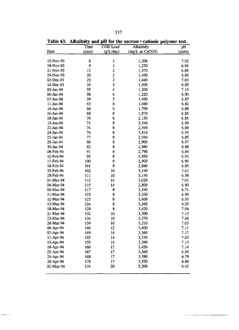
337
Table 63. Alkalinity and pH for the sucrose+cationic polymer test. Time COD Load Alkalinity pH
Date (days) (g/L/day) (mg/L as CaC03) (units)
15-NOV-93 6 1 1,200 7.02 I8-N0V-93 9 1 1,230 6.95 2I-N0V-93 12 2 1,370 6.89 29-N0V-93 20 2 1,400 6.95 02-Dec-93 23 2 1,440 7.03 14-Dec-93 35 3 1,400 6.85 03-Jan-94 55 4 1,300 7.15 06-Jan-94 58 4 1,220 6.90 07-Jan-94 59 5 1,400 6.85 ll-Jan-94 63 6 1,680 6.82 14-Jan-94 66 6 1,700 6.88 16-Jan-94 68 8 1,870 6.85 18-Jan-94 70 8 2,130 6.85 19-Jan-94 71 8 2,340 6.90 22-Jan-94 74 8 2,540 6.89 24-Jan-94 76 8 2,810 6.93 25-Jan-94 77 8 2,940 6.85 28-Jan-94 80 8 2,900 6.97 30-Jan-94 82 8 2,880 6.88 08-Feb-94 91 8 2,790 6.84 12-Feb-94 95 8 2,950 6.92 17-Feb-94 100 8 2,900 6.90 18-Feb-94 101 8 2,860 6.85 19-Feb-94 102 10 3,100 7.01 28-Feb-94 111 10 3,140 6.98 Ol-Mar-94 112 14 3,020 7.01 04-Mar-94 115 14 2,800 6.90 06-Mar-94 117 8 3,340 6.71 ll-Mar-94 122 8 3,320 6.90 12-Mar-94 123 8 3,400 6.95 13-Mar-94 124 8 3,360 6.95 18-Mar-94 129 8 3,420 7.06 21-Mar-94 132 10 3,300 7.13 23-Mar-94 134 10 3,270 7.06 28-Mar-94 139 10 3,210 7.03 04-Apr-94 146 12 3,400 7.11 07-Apr-94 149 14 3,360 7.17 ll-Apr-94 153 14 3,310 7.05 13-Apr-94 155 14 3,390 7.13 18-Apr-94 160 17 3,450 7.14 25-Apr-94 167 17 3,560 6.54 26-Apr-94 168 17 3,590 6.79 28-Apr-94 170 17 3,520 6.86 02-May-94 174 20 3,500 6.42

Table 64. Solids analysis for the sucrose+cationic polymer test. COD Load HRT MLSS MLVSS Effluent TSS Effluent VSS SRT
Date Day (g/L/day) (days) (mg/L) (% OfMLSS) (mg/L) (% of TSS) (days)
I2-N0V-93 0 1 2 17,600 55.7 I5-N0V-93 3 1 2 5,940 55.9 703 61.4 15.4 22-N0V-93 10 2 1 7,620 59.4 263 74.4 23.1 02-Dec-93 20 2 1 9,280 67.4 260 67.3 35.7 07-Dec-93 25 2 1 9,760 65.8 373 71.2 24.2 17-Dec-93 35 3 1 7,760 74.0 1,213 79.7 5.9 06-Jan-94 55 4 1 10,660 83.3 814 79.5 13.7 14-Jan-94 63 6 1 11,210 84.0 1,203 81.2 9.6 24-Jan-94 73 8 1 14,080 86.9 2,320 83.0 6.4 28-Jan-94 77 8 1 14,380 86.9 1,980 80.1 7.9 08-Feb-94 88 8 1 14,320 86.9 2,048 83.8 7.3 18-Feb-94 98 8 1 17,630 89.0 1,623 85.7 11.3 28-Feb-94 108 10 1 23,580 89.4 1,680 86.0 14.6 07-Mar-94 115 14 1 17,920 90.2 3,295 86.2 5.7 12-Mar-94 120 8 1 13,990 90.4 2,660 87.4 5.4 18-Mar-94 126 8 1 15,360 89.9 1,615 84.2 10.2 28-Mar-94 136 10 1 21,030 90.5 1,475 79.7 16.2 04-Apr-94 143 12 1 25,640 90.7 3,010 85.1 9.1 14-Apr-94 153 14 1 25,820 91.1 1,590 87.6 16.9 21-Apr-94 160 17 1 23,230 91.7 3,860 90.0 6.1 28-Apr-94 167 17 1 24,390 90.5 3,840 88.3 6.5 05-May-94 174 20 1 20,500 89.5 3,950 88.5 5.2

Table 65. COD data for the sucrose+polyDADM test. Time from Influent Effluent TCOD Effluent SCOD Start-Up HRT COD COD Load TCOD Removal SCOD Removal
Date (days) (days) (mg/L) (g/L/day) (mg/L) (%) (mg/L) (%)
18-N0V-93 6 2 2,000 1.0 557 72.2 22-NOV-93 10 1 2,000 2.0 1,574 21.3 733 63.4 02-Dec-93 20 1 2,000 2.0 902 54.9 703 64.9 07-Dec-93 25 1 2,000 2.0 1,315 34.3 944 52.8 17-Dec-93 35 1 2,000 2.0 797 60.2 671 66.5 06-Jan-94 55 1 3,000 3.0 1,376 54.1 1,262 57.9 14-Jan-94 63 1 3,000 3.0 1,692 43.6 1,250 58.3 24-Jan-94 73 1 4,000 4.0 2,325 41.9 1,804 54.9 28-Jan-94 77 1 4,000 4.0 2,933 26.7 2,133 46.7 08-Feb-94 88 1 3,000 3.0 2,069 31.0 1,580 47.3 18-Feb-94 98 1 3,000 3.0 1,917 36.1 880 70.7 28-Feb-94 108 1 3,000 3.0 1,835 38.8 771 74.3 07-Mar-94 115 1 4,000 4.0 1,918 52.1 1,328 66.8 12-Mar-94 120 1 4,000 4.0 2,205 44.9 1,376 65.6 18-Mar-94 126 1 4,000 4.0 2,065 48.4 1,251 68.7 28-Mar-94 136 1 5,000 5.0 2,687 46.3 1,576 68.5 04-Apr-94 143 1 5,000 5.0 2,387 52.3 1,676 66.5 14-Apr-94 153 1 5,000 5.0 2,654 46.9 1,478 70.4 21-Apr-94 160 1 6,000 6.0 3,043 49.3 1,889 68.5 28-Apr-94 167 1 6,000 6.0 2,883 52.0 1,143 81.0 05-May-94 174 1 8,000 8.0 3,990 50.1 3,400 57.5

340
Table 66. Biogas data for the sucrose + polyDADM test. Nominal Std Methane
HRT COD Load Methane Production Date Day (days) (g/L/day) (% of total) (L/L/day)
lO-Nov-93 0 2 1 ll-Nov-93 1 2 1 67.53 0.00 I2-N0V-93 2 2 1 67.53 0.00 I3-N0V-93 3 2 1 67.53 0.06 I4-N0V-93 4 2 1 67.53 0.09 I5-N0V-93 5 2 1 67.53 0.11 I6-N0V-93 6 2 1 67.53 0.11 I7-N0V-93 7 2 1 68.78 0.14 I8-N0V-93 8 2 1 70.03 0.14 I9-N0V-93 9 1 2 69.69 0.16 2O-N0V-93 10 1 2 69.35 0.19 2I-N0V-93 11 1 2 69.01 0.19 22-N0V-93 12 1 2 68.67 0.22 23-N0V-93 13 1 2 68.33 0.23 24-N0V-93 14 1 2 68.19 0.24 25-N0V-93 15 1 2 68.06 0.20 26-NOV-93 16 1 2 67.92 0.14 27-N0V-93 17 1 2 67.78 0.22 28-NOV-93 18 1 2 67.65 0.23 29-N0V-93 19 1 2 67.51 0.24 3O-N0V-93 20 1 2 67.94 0.23 Ol-Dec-93 21 1 2 68.37 0.29 02-Dec-93 22 1 2 68.79 0.22 03-Dec-93 23 1 2 69.22 0.20 04-Dec-93 24 1 2 69.65 0.18 05-Dec-93 25 1 2 70.08 0.28 06-Dec-93 26 1 2 70.50 0.38 07-Dec-93 27 1 2 70.93 0.30 08-Dec-93 28 1 2 71.36 0.25 09-Dec-93 29 1 2 70.60 0.23 lO-Dec-93 30 1 2 69.84 0.28 ll-Dec-93 31 1 2 69.07 0.24 12-Dec-93 32 1 2 68.31 0.29 13-Dec-93 33 1 2 67.55 0.28 14-Dec-93 34 1 2 66.79 0.27 15-Dec-93 35 1 2 66.03 0.24 16-Dec-93 36 1 2 65.26 0.24 17-Dec-93 37 1 2 64.50 0.30 18-Dec-93 38 1 2 63.74 0.25 19-Dec-93 39 1 3 62.98 0.33 20-Dec-93 40 1 3 62.22 0.38 21-Dec-93 41 1 3 61.45 0.37 22-Dec-93 42 1 3 60.69 0.31 23-Dec-93 43 1 3 59.93 0.25 24-Dec-93 44 2 3 59.84 0.32

341
Table 66. (continued). Nominal Std Methane
HRT COD Load Methane Production Date Day (days) (g/L/day) (% of total) (L/L/da
25-Dec-93 45 2 3 59.76 0.27 26-Dec-93 46 2 3 59.67 0.31 27-Dec-93 47 2 3 59.58 0.30 28-Dec-93 48 2 3 59.49 0.31 29-Dec-93 49 2 3 59.41 0.43 30-Dec-93 50 2 3 59.32 0.39 31-Dec-93 51 2 3 59.23 0.45 Ol-Jan-94 52 2 3 59.14 0.48 02-Jan-94 53 2 3 59.06 0.50 03-Jan-94 54 2 3 58.97 0.54 04-Jan-94 55 1 3 58.88 0.36 05-Jan-94 56 1 3 58.79 0.23 06-Jan-94 57 1 3 58.71 0.37 07-Jan-94 58 1 3 58.62 0.32 08-Jan-94 59 1 3 57.87 0.33 09-Jan-94 60 1 3 57.12 0.36 lO-Jan-94 61 1 3 56.37 0.40 ll-Jan-94 62 1 3 55.63 0.37 12-Jan-94 63 1 3 54.88 0.34 13-Jan-94 64 1 3 54.13 0.39 14-Jan-94 65 1 3 53.38 0.35 15-Jan-94 66 1 4 52.63 0.37 16-Jan-94 67 1 4 51.88 0.32 17-Jan-94 68 1 4 53.56 0.36 18-Jan-94 69 1 4 55.23 0.31 19-Jan-94 70 1 4 56.91 0.25 20-Jan-94 71 1 4 51.53 0.28 21-Jan-94 72 1 4 46.15 0.36 22-Jan-94 73 1 4 46.08 0.32 23-Jan-94 74 1 4 46.02 0.32 24-Jan-94 75 1 4 45.95 0.32 25-Jan-94 76 1 4 48.04 0.31 26-Jan-94 77 1 4 50.14 0.36 27-Jan-94 78 1 4 45.13 0.33 28-Jan-94 79 1 4 43.36 0.32 29-Jan-94 80 1 4 47.47 0.30 30-Jan-94 81 1 3 51.59 0.32 31-Jan-94 82 1 3 55.70 0.19 Ol-Feb-94 83 1 3 56.12 0.24 02-Feb-94 84 1 3 56.55 0.29 03-Feb-94 85 1 3 56.98 0.26 04-Feb-94 86 1 3 57.40 0.26 05-Feb-94 87 1 3 57.83 0.29 06-Feb-94 88 1 3 55.80 0.23 07-Feb-94 89 1 3 53.77 0.23

342
Table 66. (continued). Nominal Std Methane
HRT COD Load Methane Production Date Day (days) (g/L/day) (% of total) (L/L/day)
08-Feb-94 90 1 3 55.77 0.26 09-Feb-94 91 1 3 57.77 0.26 lO-Feb-94 92 1 3 59.77 0.30 ll-Feb-94 93 1 3 61.77 0.29 12-Feb-94 94 1 3 61.60 0.46 13-Feb-94 95 1 3 61.42 0.26 14-Feb-94 96 1 3 61.24 0.42 15-Feb-94 97 1 3 61.06 0.43 16-Feb-94 98 1 3 60.88 0.39 17-Feb-94 99 1 3 60.70 0.42 18-Feb-94 100 1 3 60.52 0.43 19-Feb-94 101 1 3 60.34 0.52 20-Feb-94 102 1 3 60.16 0.44 21-Feb-94 103 1 3 59.98 0.44 22-Feb-94 104 1 3 59.80 0.46 23-Feb-94 105 1 3 59.63 0.45 24-Feb-94 106 1 3 59.45 0.42 25-Feb-94 107 1 3 59.27 0.44 26-Feb-94 108 1 3 59.09 0.43 27-Feb-94 109 1 3 58.91 0.43 28-Feb-94 110 1 4 58.73 0.42 Ol-Mar-94 111 1 4 58.55 0.39 02-Mar-94 112 1 4 58.37 0.58 03-Mar-94 113 1 4 58.19 0.41 04-Mar-94 114 1 4 57.87 0.59 05-Mar-94 115 1 4 57.55 0.60 06-Mar-94 116 1 4 57.23 0.60 07-Mar-94 117 1 4 56.91 0.58 08-Mar-94 118 1 4 56.59 0.60 09-Mar-94 119 1 4 56.27 0.65 lO-Mar-94 120 1 4 55.95 0.69 ll-Mar-94 121 1 4 55.63 0.66 12-Mar-94 122 1 4 55.31 0.71 13-Mar-94 123 1 4 55.79 0.68 14-Mar-94 124 1 4 56.26 0.67 15-Mar-94 125 1 4 56.73 0.66 16-Mar-94 126 1 4 57.21 0.75 17-Mar-94 127 1 4 56.56 0.58 18-Mar-94 128 1 5 55.91 0.67 19-Mar-94 129 1 5 55.26 0.62 20-Mar-94 130 1 5 54.61 0.58 21-Mar-94 131 1 5 53.96 0.67 22-Mar-94 132 1 5 53.32 0.73 23-Mar-94 133 1 5 53.44 0.76 24-Mar-94 134 1 5 53.56 0.72

343
Table 66. (continued). Nominal Std Methane
HRT COD Load Methane Production Date Day (days) (g/L/day) (% of total) (L/L/day)
25-Mar-94 135 1 5 53.68 0.69 26-Mar-94 136 1 5 53.80 0.70 27-Mar-94 137 1 5 53.92 0.71 28-Mar-94 138 1 5 54.04 0.78 29-Mar-94 139 1 5 54.16 0.72 30-Mar-94 140 1 5 54.28 0.86 31-Mar-94 141 1 5 54.40 0.88 Ol-Apr-94 142 1 5 54.52 0.90 02-Apr-94 143 1 5 54.64 0.95 03-Apr-94 144 1 5 54.76 0.71 04-Apr-94 145 1 5 54.88 0.64 05-Apr-94 146 1 5 54.74 0.76 06-Apr-94 147 1 5 54.59 0.78 07-Apr-94 148 1 5 54.45 0.82 08-Apr-94 149 1 5 54.31 0.76 09-Apr-94 150 1 5 54.17 0.78 lO-Apr-94 151 1 5 54.03 0.94 ll-Apr-94 152 1 5 53.88 0.39 12-Apr-94 153 1 5 53.90 0.82 13-Apr-94 154 1 5 53.91 0.86 14-Apr-94 155 1 6 53.92 0.89 15-Apr-94 156 1 6 53.60 0.95 16-Apr-94 157 1 6 53.29 0.91 17-Apr-94 158 1 6 52.97 0.91 18-Apr-94 159 1 6 52.66 1.08 19-Apr-94 160 1 6 51.39 1.07 20-Apr-94 161 1 6 50.13 1.03 21-Apr-94 162 1 6 50.37 1.01 22-Apr-94 163 1 6 50.61 1.05 23-Apr-94 164 1 6 50.85 1.02 24-Apr-94 165 1 6 51.08 1.10 25-Apr-94 166 1 6 51.32 0.99 26-Apr-94 167 1 6 51.56 1.17 27-Apr-94 168 1 6 51.80 1.04 28-Apr-94 169 1 7 51.03 1.09 29-Apr-94 170 1 7 50.26 1.26 30-Apr-94 171 1 7 49.49 1.23 Ol-May-94 172 1 7 48.72 1.20 02-May-94 173 1 8 47.95 1.26 03-May-94 174 1 8 47.18 1.35 04-May-94 175 1 8 46.41 1.36 05-May-94 176 1 8 46.41 1.33 06-May-94 177 1 8 46.41 1.34

344
Table 67. Volatile acids data for the sucrose+polyDADM test. Time from Start COD Load Volatile Acids
Date (days) (g/L/day) (mg/L as acetic)
22-NOV-93 10 2.0 548 02-Dec-93 20 2.0 462 07-Dec-93 25 2.0 540 17-Dec-93 35 2.0 454 06-Jan-94 55 3.0 994 14-Jan-94 63 3.0 986 24-Jan-94 73 4.0 1,697 28-Jan-94 77 4.0 1,697 08-Feb-94 88 3.0 1,200 18-Feb-94 98 3.0 677 28-Feb-94 108 4.0 557 07-Mar-94 115 4.0 986 12-Mar-94 120 4.0 951 18-Mar-94 126 5.0 900 28-Mar-94 136 5.0 1,071 04-Apr-94 143 5.0 1,217 14-Apr-94 153 6.0 1,046 21-Apr-94 160 6.0 2,100 28-Apr-94 167 7.0 806 05-May-94 174 8.0 2,000
Table 68. Particle size analysis for the sucrose+polyDADM test. Time from Average Average
Start-up COD Load Diameter Diameter Date (days) (g/L/day) (arithmetic, /itm) (geometric, iim)
08-NOV-93 0 1 31 100 22-NOV-93 14 2 66 180 07-Dec-93 29 2 47 178 06-Jan-94 59 3 58 287 21-Jan-94 74 4 38 290 18-Feb-94 102 3 56 361 12-Mar-94 124 4 49 268 04-Apr-94 147 5 99 242 02-May-94 175 8 135 367

345
Table 69. Alkalinity and pH data for the sucrose+polyDADM test. Time COD Load Alkalinity pH
Date (days) (g/L/day) (mg/L as CaC03) (units)
15-NOV-93 5 1 1,350 7.15 I8-N0V-93 8 1 1,410 6.97 2I-N0V-93 11 2 1,400 6.95 29-N0V-93 19 2 1,300 7.01 02-Dec-93 22 2 1,360 6.97 14-Dec-93 34 2 1,300 6.98 03-Jan-94 54 3 1,300 6.88 06-Jan-94 57 3 1,300 6.68 07-Jan-94 58 3 1,400 6.75 ll-Jan-94 62 3 1,390 6.67 14-Jan-94 65 3 1,460 6.73 16-Jan-94 67 4 2,000 6.73 18-Jan-94 69 4 2,130 6.58 19-Jaii-94 70 4 2,250 6.84 22-Jan-94 73 4 2,600 6.54 24-Jan-94 75 4 2,620 6.65 25-Jan-94 76 4 2,710 6.72 28-Jan-94 79 4 2,640 6.68 30-Jan-94 81 3 2,600 6.65 08-Feb-94 90 3 2,650 6.68 12-Feb-94 94 3 2,690 6.80 17-Feb-94 99 3 2,710 6.88 18-Feb-94 100 3 2,860 6.80 19-Feb-94 101 3 2,750 6.97 28-Feb-94 110 4 2,800 6.94 Ol-Mar-94 111 4 2,790 6.88 04-Mar-94 114 4 2,860 6.78 06-Mar-94 116 4 2,840 6.89 1 l-Mar-94 121 4 2,910 6.82 12-Mar-94 122 4 2,900 6.92 13-Mar-94 123 4 3,010 6.87 18-Mar-94 128 5 2,910 6.99 2 l-Mar-94 131 5 2,940 6.91 23-Mar-94 133 5 2,870 6.87 28-Mar-94 138 5 2,780 6.85 04-Apr-94 145 5 2,690 6.88 07-Apr-94 148 5 2,760 6.83 ll-Apr-94 152 5 2,800 6.82 13-Apr-94 154 5 2,700 6.90 18-Apr-94 159 6 2,830 6.87 25-Apr-94 166 6 2,750 6.80 26-Apr-94 167 6 2,720 6.85 28-Apr-94 169 7 2,690 6.93 02-May-94 173 8 2,740 6.85

Table 70. Solids data for the sucrose+polyDADM test. Time COD Load HRT MLSS MLVSS Effluent TSS Effluent VSS SRT
Date (days) (g/L/day) (days) (mg/L) (% of MLSS) (mg/L) (% of TSS) (days)
lO-Nov-94 0 1 2 18,000 54.7 15-NOV-93 5 1 2 7,440 54.7 263 85.7 36.1 22-N0V-93 12 2 1 7,370 61.3 1,150 62.0 6.3 02-Dec-93 22 2 1 6,350 71.2 340 68.4 19.4 07-Dec-93 27 2 1 5,250 71.2 450 77.8 10.7 17-Dec-93 37 2 1 6,020 79.6 228 69.9 30.1 06-Jan-94 57 3 1 8,010 86.1 167 71.6 57.7 14-Jan-94 65 3 1 7,490 86.1 505 80.2 15.9 24-Jan-94 75 4 1 9,850 87.5 660 83.7 15.6 28-Jan-94 79 4 1 9,920 86.2 953 83.7 10.7 08-Feb-94 90 3 1 9,600 87.0 825 76.7 13.2 18-Feb-94 100 3 1 9,190 86.7 1,145 84.5 8.2 28-Feb-94 110 3 1 9,420 87.1 1,080 85.4 8.9 07-Mar-94 117 4 1 11,020 88.5 693 84.9 16.6 12-Mar-94 122 4 1 11,490 89.3 890 86.5 13.3 18-Mar-94 128 5 1 9,240 87.9 905 85.4 10.5 28-Mar-94 138 5 1 8,320 89.0 1,205 86.9 7.1 04-Apr-94 145 5 1 9,400 89.0 810 82.8 12.5 14-Apr-94 155 6 1 8,070 89.7 1,185 87.1 7.0 21-Apr-94 162 6 1 7,180 87.9 1,455 85.2 5.1 28-Apr-94 169 7 1 6,800 88.0 1,940 85.0 3.6 05-May-94 176 8 1 7,400 89.0 1,840 86.1 4.2

Table 71. COD data for the sucrose+ferric chloride test. Time from Influent Start-Up HRT COD
Date (days) (days) (mg/L)
COD Effluent TCOD Effluent SCOD Load TCOD Removal SCOD Removal
(g/L/day) (mg/L) (%) (mg/L) (%)
18-NOV-93 6 2 2,000 1.0 817 59.2 22-NOV-93 10 1 2,000 2.0 897 55.2 811 59.5 02-Dec-93 20 1 2,000 2.0 1,085 45.8 825 58.8 07-Dec-93 25 1 2,000 2.0 907 54.7 854 57.3 17-Dec-93 35 1 2,000 2.0 1,303 34.9 1,161 42.0 06-Jan-94 55 1 2,000 2.0 1,384 30.8 1,327 33.7

348
Table 72. Biogas data for the sucrose+ferric chloride test. Time from Nominal Std. Methane Start-Up HRT COD Load Methane Production
Date (days) (days) (g/L/day) (% of total) (L/L/day)
lO-Nov-93 0 2 1.0 11-Nov-93 1 2 1.0 64.15 0.04 I2-N0V-93 2 2 1.0 64.15 0.00 I3-N0V-93 3 2 1.0 64.15 0.01 I4-N0V-93 4 2 1.0 64.15 0.06 I5-N0V-93 5 2 1.0 64.15 0.03 I6-N0V-93 6 2 1.0 64.15 0.09 I7-N0V-93 7 2 1.0 62.10 0.10 I8-N0V-93 8 2 1.0 60.05 0.08 I9-N0V-93 9 1 2.0 59.40 0.09 2O-N0V-93 10 1 2.0 58.74 0.10 21-Nov-93 11 1 2.0 58.09 0.03 22-N0V-93 12 1 2.0 57.43 0.05 23-N0V-93 13 1 2.0 56.78 0.07 24-N0V-93 14 1 2.0 57.44 0.25 25-N0V-93 15 1 2.0 58.10 0.07 26-NOV-93 16 1 2.0 58.76 0.13 27-N0V-93 17 1 2.0 59.42 0.04 28-NOV-93 18 1 2.0 60.08 0.09 29-N0V-93 19 1 2.0 60.74 0.10 3O-N0V-93 20 1 2.0 62.10 0.09 Ol-Dec-93 21 1 2.0 63.46 0.28 02-Dec-93 22 1 2.0 64.82 0.13 03-Dec-93 23 1 2.0 66.18 0.12 04-Dec-93 24 1 2.0 67.53 0.16 05-Dec-93 25 1 2.0 68.89 0.22 06-Dec-93 26 1 2.0 70.25 0.09 07-Dec-93 27 1 2.0 71.61 0.12 08-Dec-93 28 1 2.0 72.97 0.18 09-Dec-93 29 1 2.0 72.07 0.11 lO-Dec-93 30 1 2.0 71.16 0.16 11-Dec-93 31 1 2.0 70.26 0.08 12-Dec-93 32 1 2.0 69.35 0.04 13-Dec-93 33 1 2.0 68.45 0.21 14-Dec-93 34 1 2.0 67.55 0.09 15-Dec-93 35 1 2.0 66.64 0.04 16-Dec-93 36 1 2.0 65.74 0.10 i7-Dec-93 37 1 2.0 64.83 0.06 18-Dec-93 38 1 2.0 63.93 0.12 19-Dec-93 39 1 2.0 63.03 0.06 20-Dec-93 40 1 2.0 62.12 0.15 21-Dec-93 41 1 2.0 61.22 0.11 22-Dec-93 42 I 2.0 60.31 0.18
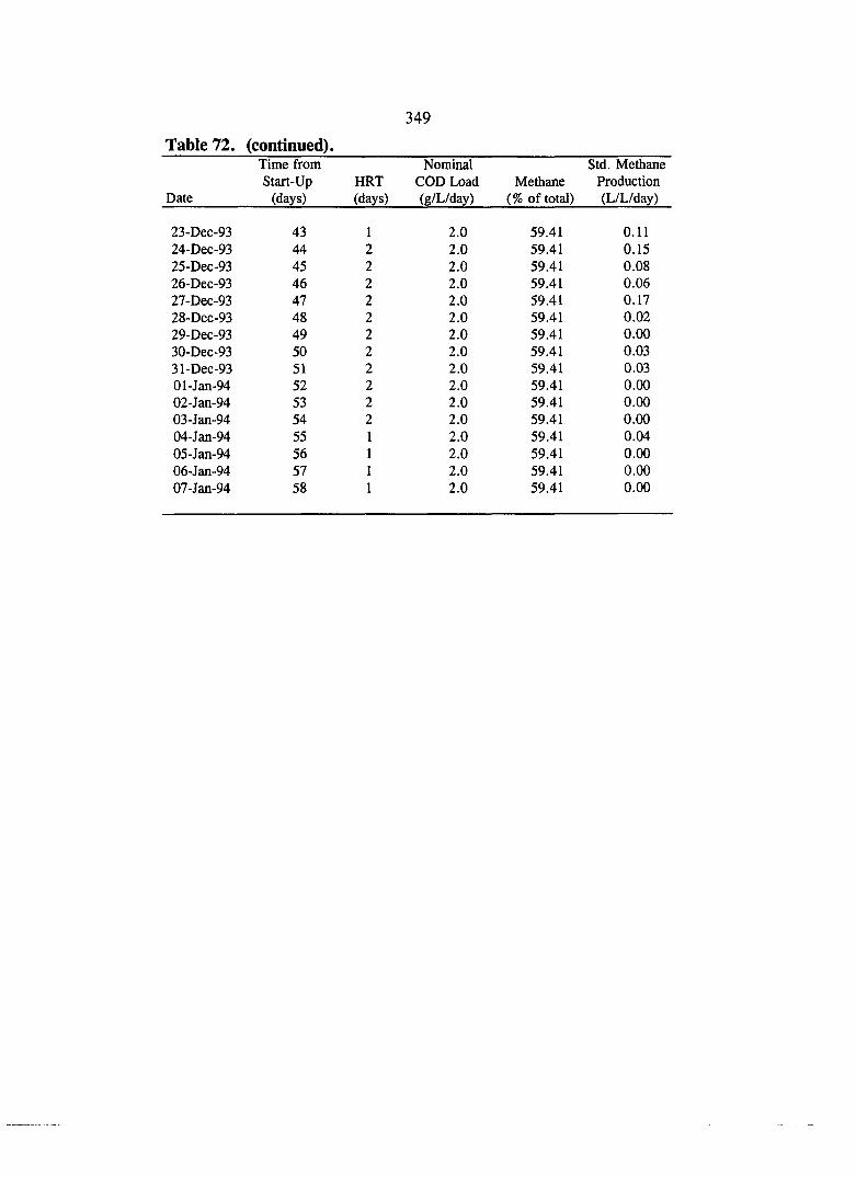
Table 72. (continued). Time from Nominal Std. Methane Start-Up HRT COD Load Methane Production
Date (days) (days) (g/L/day) (% of total) (L/L/day)
23-Dec-93 43 1 2.0 59.41 0.11 24-Dec-93 44 2 2.0 59.41 0.15 25-Dec-93 45 2 2.0 59.41 0.08 26-Dec-93 46 2 2.0 59.41 0.06 27-Dec-93 47 2 2.0 59.41 0.17 28-Dec-93 48 2 2.0 59.41 0.02 29-Dec-93 49 2 2.0 59.41 0.00 30-Dec-93 50 2 2.0 59.41 0.03 31-Dec-93 51 2 2.0 59.41 0.03 Ol-Jan-94 52 2 2.0 59.41 0.00 02-Jan-94 53 2 2.0 59.41 0.00 03-Jan-94 54 2 2.0 59.41 0.00 04-Jan-94 55 1 2.0 59.41 0.04 05-Jan-94 56 1 2.0 59.41 0.00 06-Jan-94 57 1 2.0 59.41 0.00 07-Jan-94 58 1 2.0 59.41 0.00

350
Table 73. Volatile acids data for the sucrose+ferric chloride test.
Volatile Acids (mg/L as acetic)
685 642 669 849
1,011
Time from Start-Up COD Load
Date (days) (g/L/day)
22-NOV-93 12 2.0 02-Dec-93 22 2.0 07-Dec-93 27 2.0 17-Dec-93 37 2.0 06-Jan-94 57 2.0
Table 74. Particle size analysis for the sucrose+ferric chloride test. Time from COD
Start-up Load Average Diameter Average Diameter Date (days) (g/L/day) (arithmetic, /xm) (geometric, fim)
08-NOV-93 0 1 31 100 22-NOV-93 14 2 66 223 07-Dec-93 29 2 42 204 06-Jan-94 59 2 53 160
Table 75. Alkalinity and pH for the sucrose+ferric chloride test. Time COD Load Alkalinity pH
Date (days) (g/L/day) (mg/L as CaC03) (units)
15-NOV-93 6 1 1,400 7.04 18-NOV-93 9 1 1,380 6.86 21-N0V-93 12 2 1,340 6.81 29-N0V-93 20 2 1,320 6.82 02-Dec-93 23 2 1,300 7.01 14-Dec-93 35 2 1,410 6.77 03-Jan-94 55 2 1,300 6.87 06-Jan-94 58 2 1,260 6.75

Table 76. Solids data for the sucrose+ferric chloride test. COD Load HRT MLSS MLVSS Effluent TSS Effluent VSS SRT
Date Day (g/L/day) (days) (mg/L) (% of MLSS) (mg/L) (%ofTSS) (days)
12-NOV-93 0 1 2 17,880 54.3 15-NOV-93 3 1 2 8,310 54.6 265 72.1 47.5 22-N0V-93 10 2 1 6,270 61.4 220 58.0 30.2 02-Dec-93 20 2 1 6,410 71.1 420 66.1 16.4 07-Dec-93 25 2 1 6,950 71.5 173 55.0 52.2 17-Dec-93 35 2 1 7,720 71.9 255 66.7 32.6 06-Jan-94 55 2 1 7,580 76.4 144 70.7 56.9

Table 77. COD data for the beef/glucose control test. Influent Effluent TCOD Effluent SCOD
DAY HRT COD COD Load TCOD Removal SCOD Removal Date (days) (days) (mg/L) (g/L/day) (mg/L) (%) (mg/L) (%)
24-Jan-94 7 2 2,000 1.0 873 56.4 686 65.7 28-Jan-94 11 1 2,000 2.0 1,196 40.2 937 53.2 08-Feb-94 22 1 2,000 2.0 1,693 15.4 767 61.7 18-Feb-94 32 2 5,500 2.8 2,803 49.0 1,938 64.8 28-Feb-94 42 2 4,000 2.0 2,510 37.3 1,835 54.1 07-Mar-94 49 1 2,000 2.0 1,853 7.4 788 60.6 12-Mar-94 54 1 2,000 2.0 1,667 16.7 837 58.2 18-Mar-94 60 1 2,000 2.0 1,207 39.7 764 61.8 28-Mar-94 70 1 3,000 3.0 1,533 48.9 1,039 65.4 04-Apr-94 77 1 3,000 3.0 1,488 50.4 803 73.2 14-Apr-94 87 1 4,000 4.0 2,336 41.6 1,415 64.6 21-Apr-94 94 1 4,000 4.0 1,981 50.5 1,300 67.5 28-Apr-94 101 1 4,000 4.0 1,695 57.6 820 79.5 05-May-94 108 1 6,000 6.0 3,240 46.0 1,580 73.7

353
Table 78. Biogas data for the beef/glucose control test. Nominal Std. Methane
HRT COD Load Methane Production Date Day (days) (g/L/day) (% of total) (L/L/day)
17-Jan-94 0 2 1.0 18-Jan-94 1 2 1.0 77.91 0.02 19-Jan-94 2 2 1.0 77,91 0.08 20-Jan-94 3 2 I.O 82.16 0.11 21-Jan-94 4 2 1.0 86.41 0.08 22-Jan-94 5 2 1.0 83.98 0.06 23-Jan-94 6 2 1.0 81.55 0.09 24-Jan-94 7 2 1.0 79.12 0.14 25-Jan-94 8 2 1.0 80.03 0.20 26-Jan-94 9 1 2.0 80.94 0.19 27-Jan-94 10 1 2.0 76.91 0.23 28-Jan-94 11 1 2.0 74.14 0.22 29-Jan-94 12 1 2.0 74.18 0.26 30-Jan-94 13 1 2.0 74.22 0.31 31-Jan-94 14 1 2.0 74.26 0.31 Ol-Feb-94 15 1 2.0 75.11 0.29 02-Feb-94 16 1 2.0 75.96 0.29 03-Feb-94 17 1 2.0 76.82 0.25 04-Feb-94 18 1 2.0 77.67 0.36 05-Feb-94 19 1 2.0 78.52 0.29 06-Feb-94 20 1 2.0 78.59 0.24 07-Feb-94 21 1 2.0 78.66 0.25 08-Feb-94 22 1 2.0 76.97 0.33 09-Feb-94 23 1 2.0 75.28 0.30 lO-Feb-94 24 1 2.0 73.58 0.26 ll-Feb-94 25 1 2.0 71.89 0.28 12-Feb-94 26 1 2.0 71.90 0.29 13-Feb-94 27 1 2.0 71.92 0.17 14-Feb-94 28 1 2.0 71.93 0.17 15-Feb-94 29 2 2.0 71.95 0.21 16-Feb-94 30 2 2.0 71.96 0.16 17-Feb-94 31 2 2.0 71.98 0.18 18-Feb-94 32 2 2.0 71.99 0.17 19-Feb-94 33 2 2.0 72.01 0.17 20-Feb-94 34 2 2.0 72.02 0.19 21-Feb-94 35 2 2.0 72.03 0.21 22-Feb-94 36 2 2.0 72.05 0.19 23-Feb-94 37 2 2.0 72.06 0.20 24-Feb-94 38 2 2.0 72.08 0.19 25-Feb-94 39 2 2.0 72.09 0.16 26-Feb-94 40 2 2.0 72.11 0.24 27-Feb-94 41 2 2.0 72.12 0.21 28-Feb-94 42 2 2.0 72.14 0.25 Ol-Mar-94 43 1 2.0 72.15 0.13 02-Mar-94 44 1 2.0 72.17 0.22

354
Table 78. (continued). Nominal Std. Methane
HRT COD Load Methane Production Date Day (days) (g/L/day) (% of total) (L/L/day)
03-Mar-94 45 1 2.0 72.18 0.18 04-Mar-94 46 1 2.0 72.18 0.18 05-Mar-94 47 1 2.0 72.19 0.14 06-Mar-94 48 1 2.0 72.19 0.22 07-Mar-94 49 1 2.0 72.20 0.17 08-Mar-94 50 1 2.0 72.20 0.18 09-Mar-94 51 1 2.0 72.21 0.20 lO-Mar-94 52 1 2.0 72.21 0.27 ll-Mar-94 53 1 2.0 72.22 0.15 12-Mar-94 54 1 2.0 72.22 0.18 13-Mar-94 55 1 2.0 72.39 0.23 14-Mar-94 56 1 2.0 72.56 0.28 15-Mar-94 57 1 2.0 72.72 0.20 16-Mar-94 58 1 2.0 72.89 0.27 17-Mar-94 59 1 2.0 71.89 0.26 18-Mar-94 60 1 2.0 70.88 0.26 19-Mar-94 61 I 3.0 69.88 0.30 20-Mar-94 62 1 3.0 68.88 0.23 21-Mar-94 63 1 3.0 67.87 0.33 22-Mar-94 64 1 3.0 66.87 0.43 23-Mar-94 65 1 3.0 67.09 0.42 24-Mar-94 66 1 3.0 67.31 0.46 25-Mar-94 67 1 3.0 67.54 0.35 26-Mar-94 68 1 3.0 67.76 0.44 27-Mar-94 69 1 3.0 67.98 0.42 28-Mar-94 70 1 3.0 68.20 0.42 29-Mar-94 71 1 3.0 68.43 0.50 30-Mar-94 72 1 3.0 68.65 0.48 31-Mar-94 73 1 3.0 68.87 0.63 Ol-Apr-94 74 1 3.0 69.09 0.53 02-Apr-94 75 1 3.0 69.32 0.55 03-Apr-94 76 1 3.0 69.54 0.55 04-Apr-94 77 1 3.0 69.76 0.62 05-Apr-94 78 1 3.0 69.19 0.68 06-Apr-94 79 1 4.0 68.61 0.78 07-Apr-94 80 1 4.0 68.04 0.79 08-Apr-94 81 1 4.0 67.47 0.83 09-Apr-94 82 1 4.0 66.90 0.78 lO-Apr-94 83 1 4.0 66.32 0.85 ll-Apr-94 84 1 4.0 65.75 0.28 12-Apr-94 85 1 4.0 65.88 0.63 13-Apr-94 86 1 4.0 66.00 0.61 14-Apr-94 87 1 4.0 66.13 0.51 15-Apr-94 88 1 4.0 66.00 0.44 16-Apr-94 89 1 4.0 65.87 0.59

355
Table 78. (continued). Nominal Std. Methane
HRT COD Load Methane Production Date Day (days) (g/L/day) (% of total) (L/L/day)
17-Apr-94 90 1 4.0 65.74 0.48 18-Apr-94 91 1 4.0 65.61 0.48 19-Apr-94 92 1 4.0 64.37 0.54 20-Apr-94 93 1 4.0 63.12 0.51 21-Apr-94 94 1 4.0 63.97 0.46 22-Apr-94 95 1 4.0 64.83 0.60 23-Apr-94 96 1 4.0 65.68 0.54 24-Apr-94 97 1 4.0 66.54 0.54 25-Apr-94 98 1 4.0 67.39 0.55 26-Apr-94 99 1 4.0 68.25 0.59 27-Apr-94 100 1 4.0 69.10 0.60 28-Apr-94 101 1 4.0 69.95 0.72 29-Apr-94 102 1 5.0 69.84 0.91 30-Apr-94 103 1 5.0 69.72 0.96 Ol-May-94 104 1 5.0 69.60 0.98 02-May-94 105 1 5.0 69.48 1.05 03-May-94 106 1 6.0 69.36 1.14 04-May-94 107 1 6.0 68.27 1.26 05-May-94 108 1 6.0 68.27 1.23 06-May-94 109 1 6.0 68.27 1.26

356
Table 79. Volatile acids data for the beef/glucose control test. Time from Start COD Load Volatile Acids
(days) (g/L/day) (mg/L as acetic) Date
24-Jan-94 7 1.0 497 28-Jan-94 11 2.0 634 08-Feb-94 22 2.0 523 18-Feb-94 32 2.8 1,603 28-Feb-94 42 2.0 1,397 07-Mar-94 49 2.0 669 12-Mar-94 54 2.0 677 18-Mar-94 60 2.0 523 28-Mar-94 70 3.0 711 04-Apr-94 77 3.0 617 14-Apr-94 87 4.0 943 21-Apr-94 94 4.0 883 28-Apr-94 101 4.0 557 05-May-94 108 6.0 987
Table 80. Particle size analysis for the beef/glucose control test. Time from COD
Start-up Load Average Diameter Average Diameter Date (days) (g/L/day) (arithmetic, /xm) (geometric, /xm)
17-Jan-94 0 1 34 231 18-Feb-94 32 2 34 330 12-Mar-94 54 2 40 420 04-Apr-94 77 3 53 440 02-May-94 105 6 111 490

357
Table 81. Alkalinity and pH for the beef/glucose control test. Time COD Load Alkalinity pH
Date (days) (g/L/day) (mg/L as CaC03) (units)
18-Jan-94 1 1 2,650 7.63 19-Jan-94 2 1 2,710 7.44 22-Jan-94 5 1 2,690 7.32 24-Jan-94 7 1 2,640 7.31 25-Jan-94 8 1 2,600 7.22 28-Jan-94 11 2 2,700 7.11 30-Jan-94 13 2 2,650 7.03 08-Feb-94 22 2 2,700 6.98 12-Feb-94 26 3 2,750 7.00 17-Feb-94 31 3 2,800 6.86 18-Feb-94 32 3 2,790 6.90 19-Feb-94 33 4 2,780 7.01 28-Feb-94 42 3 2,690 7.00 Ol-Mar-94 43 3 2,750 7.05 04-Mar-94 46 3 2,810 7.03 06-Mar-94 48 3 2,710 7.14 ll-Mar-94 53 3 2,750 7.06 12-Mar-94 54 3 2,700 7.16 13-Mar-94 55 3 2,720 7.08 18-Mar-94 60 4 2,730 7.13 21-Mar-94 63 4 2,790 7.08 23-Mar-94 65 4 2,850 6.99 28-Mar-94 70 4 2,810 6.89 04-Apr-94 77 5 2,790 7.02 07-Apr-94 80 6 2,860 6.97 ll-Apr-94 84 6 2,820 6.93 13-Apr-94 86 6 2,850 6.93 18-Apr-94 91 6 2,760 6.93 25-Apr-94 98 6 2,730 6.96 26-Apr-94 99 6 2,790 7.00 28-Apr-94 101 7 2,810 7.04 02-May-94 105 8 2,800 7.08

Table 82. Solids analysis for beef/glucose control test. Date Day COD Load HRT MLSS MLVSS Effluent TSS Effluent VSS SRT
(g/L/day) (days) (mg/L) (% of MLSS) (mg/L) (% of TSS) (days)
17-Jan-94 0 1 2 24,953 57.0 24-Jan-94 7 1 2 7,460 57.0 233 52.7 69.3 28-Jan-94 11 2 1 8,210 61.0 418 51.5 23.3 08-Feb-94 22 2 1 6,740 63.4 1,053 70.8 5.7 18-Feb-94 32 2 2 5,600 77.5 803 71.4 15.1 28-Feb-94 42 2 2 8,560 82.3 715 73.8 26.7 07-Mar-94 49 2 1 6,800 83.4 763 80.0 9.3 12-Mar-94 54 2 1 6,290 83.2 552 81.2 11.7 18-Mar-94 60 2 1 6,510 83.8 438 74.3 16.8 28-Mar-94 70 3 1 6,390 83.9 488 73.9 14.9 04-Apr-94 77 3 1 6,290 84.9 640 77.8 10.7 14-Apr-94 87 4 1 3,720 81.2 755 79.8 5.0 21-Apr-94 94 4 1 4,550 82.5 663 84.6 6.7 28-Apr-94 101 4 1 6,480 82.0 888 83.0 7.2 05-May-94 108 6 1 6,900 83.1 925 82.3 7.5

Table 83. COD data for the beef/glucose+cationic polymer test. Influent Effluent TCOD Effluent SCOD
DAY HRT COD COD Load TCOD Removal SCOD Removal Date (days) (days) (mg/L) (g/L/day) (mg/L) (%) (mg/L) (%)
24-Jan-94 7 2 2,000 1.0 373 81.4 246 87.7 28-Jan-94 11 1 2,000 2.0 556 72.2 459 77.1 08-Feb-94 22 1 2,000 2.0 602 69.9 459 77.1 18-Feb-94 32 1 3,500 3.5 674 80.7 443 87.3 28-Feb-94 42 1 4,500 4.5 2,319 48.5 1,681 62.6 07-Mar-94 49 1 6,500 6.5 2,422 62.7 2,247 65.4 12-Mar-94 54 1 3,000 3.0 1,354 54.9 1,256 58.1 18-Mar-94 60 1 3,000 3.0 975 67.5 815 72.8 28-Mar-94 70 1 4,000 4.0 896 77.6 767 80.8 {)4-Apr-94 77 1 5,000 5.0 1,956 60.9 460 90.8 14-Apr-94 87 1 6,500 6.5 4,553 30.0 3,088 52.5 21-Apr-94 94 1 6,500 6.5 3,453 46.9 2,013 69.0 28-Apr-94 101 1 6,500 6.5 2,438 62.5 1,733 73.3 05-May-94 108 1 8,000 8.0 3,500 56.3 3,100 61.3

360
Table 84. Biogas data for the beef/glucose+cationic polymer test. Nominal Std. Methane
HRT COD Load Methane Production Date Day (days) (g/L/day) (% of total) (L/L/day)
17-Jan-94 0 2 1.0 18-Jan-94 1 2 1.0 80.06 0.08 19-Jan-94 2 2 1.0 80.06 0.16 20-Jan-94 3 2 1.0 83.13 0.18 21-Jan-94 4 2 1.0 86.20 0.25 22-Jan-94 5 2 1.0 84.93 0.25 23-Jan-94 6 2 1.0 83.65 0.26 24-Jan-94 7 2 1.0 82.38 0.24 25-Jan-94 8 2 1.0 81.52 0.27 26-Jan-94 9 1 2.0 80.65 0.34 27-Jan-94 10 1 2.0 78.29 0.45 28-Jan-94 11 1 2.0 78.02 0.50 29-Jan-94 12 1 2.0 77.93 0.43 30-Jan-94 13 1 2.0 77.84 0.46 31-Jan-94 14 1 2.0 77.75 0.48 Ol-Feb-94 15 1 2.0 77.59 0.50 02-Feb-94 16 1 2.0 77.44 0.61 03-Feb-94 17 1 2.0 77.28 0.68 04-Feb-94 18 1 2.0 77.13 0.47 05-Feb-94 19 1 2.0 76.97 0.53 06-Feb-94 20 1 2.0 77.06 0.45 07-Feb-94 21 1 2.0 77.15 0.49 08-Feb-94 22 1 2.0 77.60 0.68 09-Feb-94 23 1 3.0 78.05 0.72 lO-Feb-94 24 1 3.0 78.49 0.78 ll-Feb-94 25 1 3.0 78.94 0.96 12-Feb-94 26 1 3.0 78.24 0.92 13-Feb-94 27 1 3.0 77.54 0.91 14-Feb-94 28 1 3.0 76.84 0.53 15-Feb-94 29 1 4.5 76.14 1.14 16-Feb-94 30 1 4.5 75.44 0.99 17-Feb-94 31 1 4.5 74.74 1.01 18-Feb-94 32 1 4.5 74.04 0.93 19-Feb-94 33 1 4.5 73.34 1.18 20-Feb-94 34 1 4.5 72.64 1.08 21-Feb-94 35 1 4.5 71.94 1.00 22-Feb-94 36 1 4.5 71.25 1.12 23-Feb-94 37 1 4.5 70.55 1.12 24-Feb-94 38 1 4.5 69.85 1.01 25-Feb-94 39 1 4.5 69.15 0.97 26-Feb-94 40 1 4.5 68.45 0.71 27-Feb-94 41 1 4.5 67.75 0.53 28-Feb-94 42 1 4.5 67.05 0.37 Ol-Mar-94 43 2 3.0 66.35 0.26 02-Mar-94 44 2 3.0 65.65 0.32

ON Vi > t3
— O O O O O O _ U> ts)
•-» »-! »-l •-! -t •-t •-t •t •t •-1 "I •-I »-l »-i "-1 NO VJD NJO NO N J D vo vb JD NO >b VD NO NJD NO
4:^ 4:^ 4^ 4:^ 4^ 4:^ 4^ 4^ 4^ 4^ 4:^ 4^
00 00 00 00 00 00 00 00 00 00 -J --O •-J -J o 00 -4 ON Ui 4^ UJ ro H- o vO 00 ON Ui 4^
O to NO N) 00
N) •-J
K) ON
K) U% to 4 to U> to to to to o Co 00 ON U) to O O VO O 00 o o On S o O U) k k k p •t
k •-1
k •1
2 £5 k B5 k >-t
2 2 2 2 p •-I
2 p •-I
2 p •-*
2 p 2 £5
2 2 2 p •-I
2 2 p •-t
2 p 2 p »-t
k p »-i k p •1
k k e? k p •-!
2 ej
<> vo 45>. VD 4!». NO 4 NO 4 vb 4 b 4 b 4
>b 4 b 4 b 4 vb 4 b 4
b> 4 b 4
vb 4s>' vb 4 b 4 b 4 b 4 NO 4 b 4: b» 4 Nb 4
NO 4:». NO 4 b 4^
O v O O O - - J O N U » 4 ^ U > t O » — O v o o O ' - J O N < - ' » 5 > ' W S ) ^ O v O O O - - 4 0 \ t ^ 4 : i ' U i N > ^ O v O O O - - J a s C n
N> N> N) N) N>
a \ O N a \ O v O \ O s O N O N a N a \ a \ L n L f ) ^ U l U i U i U t 4 ^ 4 : ^ ^ - P k . 4 ^ 4 ^ 4 ^ 4 : ) . ^ 4 ^ 4 ^ U d U J U > U > ( > J ( > J U J U > L » ^ U > U > U J U ^ ( > ^ L » J U } o o o o o o o o o o o o o o o o o o b o o o o o o o o o o o o o o o o o o o o o o o o o o
U i U i Lr\ ON
U i Ov Lfi On O n U i t-A t-n L n L n 'sJi U l U i U i LA
0 \ LA On
Ln Ln U\ ON LA On LA LA LA LA LA 4 LA LA LA -J LA 00 LA
)0
4 00 ON to U) b 00 00 L/I to 00 Ln Ui bo to t- o 00 VO 8 b LA 4 b ON La NO to 00 io
On to 4 s ON O n ON 0\ to O n to O n u> ON U) ON Ui O n U) O n UJ 0\ Lh> ON LO ON U) O n ON LO ON to ON to O n to O n ON to O n to to to ON UJ b LA 4i
On 00 •-J to 00 ON NO LA to \D 00 O
ON 00 LA LA to to VO 5 g 00 bv On LA L»J 4i. O
N> •-J
O o o p P o p p p LA 4 LA 4i 00 LA 4 4 00 o to 00 NO 00
H - O O O O O O O O O O
- - i O O V O U i O v O b J N > \ O U >
p p p p p p p p p p p p p u> to to to U) u> Iti UJ L»J L»J to 00 00 VO 00 o LA LA LA 00 ON 00 o

362
Table 84. (continued). Nominal Std. Methane
HRT COD Load Methane Production Date Day (days) (g/L/day) (% of total) (L/L/day)
17-Apr-94 90 1 6.0 59.39 0.50 18-Apr-94 91 1 6.0 60.27 0.53 19-Apr-94 92 1 6.0 59.83 0.65 20-Apr-94 93 1 6.0 59.40 0.65 21-Apr-94 94 1 6.0 59.51 0.66 22-Apr-94 95 1 6.0 59.62 0.57 23-Apr-94 96 1 6.0 59.74 0.71 24-Apr-94 97 1 6.0 59.85 0.64 25-Apr-94 98 1 6.0 59.96 0.61 26-Apr-94 99 1 6.0 60.07 0.69 27-Apr-94 100 1 6.0 60.19 0.67 28-Apr-94 101 1 6.0 60.30 0.90 29-Apr-94 102 1 7.0 59.90 0.91 30-Apr-94 103 1 7.0 59.50 0.92 Ol-May-94 104 1 7.0 59.10 0.95 02-May-94 105 1 7.0 58.69 0.92 03-May-94 106 1 8.0 58.29 0.89 04-May-94 107 1 8.0 57.38 1.06 05-May-94 108 1 8.0 57.38 0.83 06-May-94 109 1 8.0 57.38 1.02

Table 85. Volatile acids data for the beef/glucose+cationic polymer test.
Date Time from Start
(days) COD Load (g/L/day)
Volatile Acids (mg/L as acetic)
24-Jan-94 7 1.0 103 28-Jan-94 11 2.0 240 08-Feb-94 22 2.0 291 18-Feb-94 32 3.5 274 28-Feb-94 42 4.5 1,269 07-Mar-94 49 3.0 1,723 12-Mar-94 54 3.0 1,011 18-Mar-94 60 3.0 634 28-Mar-94 70 4.0 86 04-Apr-94 77 5.0 334 14-Apr-94 87 6.0 1,971 21-Apr-94 94 6.0 1,371 28-Apr-94 101 6.0 1,183 05-May-94 108 8.0 2,200
Table 86. Particle size analysis for the beef/glucose+cationic polymer test. Time from COD
Start-up Load Average Diameter Average Diameter Date (days) (g/L/day) (arithmetic, /xm) (geometric, /^m)
17-Jan-94 0 1 34 189 18-Feb-94 32 3 56 399 12-Mar-94 54 3 48 686 04-Apr-94 77 5 114 509 02-May-94 105 8 301 885

364
Table 87. Alkalinity and pH for the beef/glucose+cationic polymer test. Time from Start-Up COD Load Alkalinity pH
Date (days) (g/L/day) (mg/L as CaC03) (units)
18-Jan-94 1 1 2,600 7.57 19-Jan-94 2 1 2,500 7.40 22-Jan-94 5 1 2,750 7.37 24-Jan-94 7 1 2,650 7.35 25-Jan-94 8 1 2,490 7.22 28-Jan-94 11 2 2,620 7.23 30-Jan-94 13 2 2,500 7.11 08-Feb-94 22 2 2,590 7.01 12-Feb-94 26 3 2,640 7.02 17-Feb-94 31 3 2,580 6.96 18-Feb-94 32 3 2,610 6.95 19-Feb-94 33 4 2,540 7.06 28-Feb-94 42 3 2,600 6.88 Ol-Mar-94 43 3 2,500 6.94 04-Mar-94 46 3 2,550 6.93 06-Mar-94 48 3 2,650 6.93 ll-Mar-94 53 3 2,690 7.02 12-Mar-94 54 3 2,710 7.08 13-Mar-94 55 3 2,650 7.04 18-Mar-94 60 4 2,700 7.11 21-Mar-94 63 4 2,780 7.03 23-Mar-94 65 4 2,790 7.00 28-Mar-94 70 4 2,750 6.96 04-Apr-94 77 5 2,850 7.11 07-Apr-94 80 6 2,890 7.00 ll-Apr-94 84 6 2,990 6.79 13-Apr-94 86 6 3,010 6.80 18-Apr-94 91 6 3,110 6.86 25-Apr-94 98 6 2,960 6.82 26-Apr-94 99 6 3,000 6.86 28-Apr-94 101 7 3,150 6.94 02-May-94 105 8 3,200 6.96
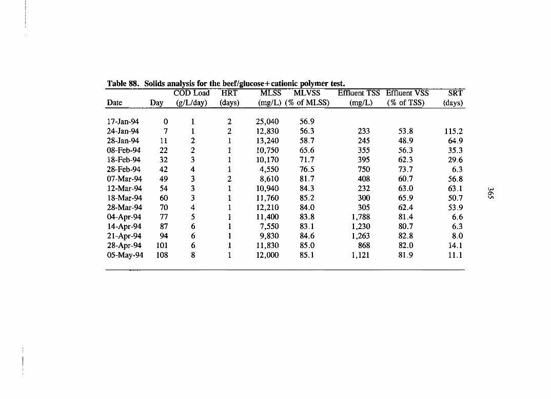
Table 88. Solids analysis for the beef/glucose+cationic polymer test. COD Load HRT MLSS MLVSS Effluent TSS Effluent VSS SRT
Date Day (g/L/day) (days) (mg/L) (% of MLSS) (mg/L) (% of TSS) (days)
17-Jan-94 0 1 2 25,040 56.9 24-Jan-94 7 1 2 12,830 56.3 233 53.8 115.2 28-Jan-94 11 2 1 13,240 58.7 245 48.9 64.9 08-Feb-94 22 2 1 10,750 65.6 355 56.3 35.3 18-Feb-94 32 3 1 10,170 71.7 395 62.3 29.6 28-Feb-94 42 4 1 4,550 76.5 750 73.7 6.3 07-Mar-94 49 3 8,610 81.7 408 60.7 56.8 12-Mar-94 54 3 1 10,940 84.3 232 63.0 63.1 18-Mar-94 60 3 1 11,760 85.2 300 65.9 50.7 28-Mar-94 70 4 1 12,210 84.0 305 62.4 53.9 04-Apr-94 77 5 1 11,400 83.8 1,788 81.4 6.6 14-Apr-94 87 6 1 7,550 83.1 1,230 80.7 6.3 21-Apr-94 94 6 1 9,830 84.6 1,263 82.8 8.0 28-Apr-94 101 6 1 11,830 85.0 868 82.0 14.1 05-May-94 108 8 1 12,000 85.1 1,121 81.9 11.1

366
Table 89. SMA test with the PAC-enhanced ASBR, day 158. Time of Time Cumulative Cumulative Cumulative
Day Elapsed Gas Methane Methane Methane (hr:min) (min) (liters) (% of total) (liters) (mL/g MLVSS)
02:01 PM 0 0.00 57.19 0.00 0.00 02:05 PM 4 0.13 57.60 0.07 0.26 02:07 PM 6 0.40 58.02 0.23 0.80 02:09 PM 8 0.74 58.43 0.43 1.49 02:11 PM 10 1.23 58.84 0.72 2.49 02:13 PM 12 1.66 58.39 0.97 3.37 02:15 PM 14 2.06 57.94 1.20 4.18 02:17 PM 16 2.42 57.49 1.41 4.90 02:19 PM 18 2.73 57.04 1.59 5.52 02:21 PM 20 3.02 56.58 1.75 6.10 02:23 PM 22 3.29 56.13 1.90 6.63 02:25 PM 24 3.54 55.68 2.04 7.11 02:27 PM 26 3.80 55.23 2.19 7.61 02:29 PM 28 4.06 54.20 2.33 8.11 02:31 PM 30 4.32 53.16 2.47 8.60 02:33 PM 32 4.56 52.13 2.59 9.04 02:35 PM 34 4.78 51.09 2.71 9.43 02:37 PM 36 5.01 50.06 2.82 9.84 02:39 PM 38 5.23 49.02 2.93 10.22 02:41 PM 40 5.45 47.99 3.04 10.59 02:43 PM 42 5.68 46.95 3.15 10.97 02:45 PM 44 5.90 45.92 3.25 11.32 02:47 PM 46 6.11 45.40 3.35 11.66 02:49 PM 48 6.32 44.88 3.44 11.99 02:51 PM 50 6.53 44.36 3.54 12.31 02:53 PM 52 6.75 43.84 3.63 12.65 02:55 PM 54 6.97 43.32 3.73 12.98 02:57 PM 56 7.19 42.80 3.82 13.31 02:59 PM 58 7.39 42.28 3.91 13.61 03:01 PM 60 7.60 41.76 4.00 13.92 03:03 PM 62 7.76 41.24 4.06 14.15 03:05 PM 64 7.94 40.72 4.14 14.41 03:07 PM 66 8.10 40.20 4.20 14.63 03:09 PM 68 8.28 40.04 4.27 14.88 03:12 PM 71 8.54 39.87 4.38 15.24 03:15 PM 74 8.79 39.71 4.48 15.59 03:18 PM 77 9.03 39.54 4.57 15.92 03:21 PM 80 9.27 39.38 4.67 16.25 03:25 PM 84 9.61 39.21 4.80 16.72 03:29 PM 88 9.96 39.05 4.94 17.19 03:33 PM 92 10.29 39.23 5.07 17.64 03:37 PM 96 10.64 39.40 5.20 18.12 03:41 PM 100 10.95 39.58 5.33 18.55
Notes: substrate = sucrose; MLVSS = 23,933 mg/L; F/M = 0.25.

Table 89. (continued). Time of Time Cumulative Cumulative Cumulative
Day Elapsed Gas Methane Methane Methane (hr:min) (min) (liters) (% of total) (liters) (mL/g MLVSS)
03:46 PM 105 11.37 39.75 5.49 19.13 03:50 PM 109 11.68 39.93 5.62 19.56 03:55 PM 114 12.09 40.10 5.78 20.13 04:00 PM 119 12.49 40.28 5.94 20.69 04:05 PM 124 12.91 40.45 6.11 21.28 04:10 PM 129 13.33 40.63 6.28 21.87 04:15 PM 134 13.74 41.16 6.45 22.46 04:20 PM 139 14.14 41.70 6.62 23.03 04:25 PM 144 14.55 42.23 6.79 23.63 04:31 PM 150 15.04 42.76 7.00 24.36 04:37 PM 157 15.56 43.29 7.22 25.14 04:47 PM 167 16.37 43.83 7.57 26.37 04:53 PM 172 16.81 44.36 7.77 27.04 04:59 PM 178 17.28 44.89 7.98 27.77 05:02 PM 181 17.52 45.42 8.08 28.15 05:10 PM 189 18.14 45.95 8.37 29.14 05:21 PM 200 19.06 46.48 8.79 30.62 05:30 PM 209 19.80 47.01 9.14 31.82 05:41 PM 220 20.57 47.53 9.50 33.09 05:51 PM 230 21.33 48.06 9.87 34.35 06:00 PM 239 22.95 48.59 10.65 37.08 06:10 PM 249 23.72 49.12 11.02 38.39 06:20 PM 259 24.48 49.65 11.40 39.70 06:25 PM 264 24.82 50.18 11.57 40.29 06:31 PM 270 25.26 50.55 11.79 41.06 06:36 PM 275 25.62 50.92 11.97 41.69 06:41 PM 280 25.99 51.30 12.16 42.35 06:48 PM 287 26.51 51.67 12.43 43.28 06:54 PM 293 26.92 52.04 12.64 44.02 07:01 PM 300 27.42 52.41 12.90 44.93 07:08 PM 307 27.90 52.79 13.16 45.81 07:14 PM 313 28.31 53.16 13.37 46.57 07:23 PM 322 28.94 53.61 13.71 47.74 07:31 PM 330 29.51 54.05 14.02 48.81 07:38 PM 337 29.98 54.50 14.27 49.70 07:49 PM 348 30.70 54.95 14.67 51.07 07:55 PM 354 31.09 55.39 14.88 51.82 08:08 PM 367 31.95 55.84 15.36 53.48 08:19 PM 378 32.68 56.29 15.77 54.91 08:28 PM 387 33.25 56.74 16.09 56.03 08:35 PM 394 33.69 57.18 16.34 56.90 08:39 PM 398 33.93 57.63 16.48 57.38 08:46 PM 405 34.36 58.08 16.73 58.25 09:06 PM 425 35.60 58.54 17.45 60.77 09:11 PM 430 35.89 58.99 17.62 61.36

Table 89. (continued). Time of Time Cumulative Cumulative Cumulative
Day Elapsed Gas Methane Methane Methane (hr:min) (min) (liters) (% of total) (liters) (mL/g MLVSS)
09:52 PM 471 38.20 59.62 18.99 66.13 09:59 PM 478 38.58 60.25 19.22 66.92 11:08 PM 547 41.49 61.02 20.98 73.07 11:16 PM 555 41.70 61.79 21.11 73.52 11:24 PM 563 41.89 62.03 21.23 73.93 11:37 PM 576 42.18 62.27 21.41 74.55 11:47 PM 586 42.40 62.51 21.55 75.03 11:56 PM 595 42.57 62.75 21.66 75.40 12:06 AM 605 42.77 62.99 21.78 75.84 12:17 AM 616 42.98 63.02 21.91 76.30 12:31 AM 630 43.25 63.05 22.08 76.89 12:48 AM 647 43.56 63.08 22.28 77.57

Table 90. SMA test with the PAC-enhanced ASBR, day 169. Time of Time Cumulative Cumulative Cumulative
Day Elapsed Gas Methane Methane Methane (hr:mm) (min) (liters) (% of total) (liters) (mL/g MLVSS)
10:54 AM 0 0.00 57.86 0.00 0.00 10:56 AM 2 0.00 57.80 0.00 0.00 10:58 AM 4 0.00 57.74 0.00 0.00 11:00 AM 6 0.09 57.68 0.05 0.15 11:02 AM 8 0.33 57.62 0.19 0.57 11:04 AM 10 0.48 57.52 0.28 0.82 11:06 AM 12 0.58 57.43 0.33 0.99 11:08 AM 14 0.71 57.33 0.41 1.22 11:10 AM 16 0.78 57.23 0.45 1.33 11:12 AM 18 0.86 57.14 0.49 1.47 11:14 AM 20 0.94 57.04 0.54 1.61 11:16 AM 22 1.01 56.94 0.58 1.72 11:18 AM 24 1.07 56.85 0.61 1.83 11:20 AM 26 1.13 56.75 0.65 1.93 11:22 AM 28 1.17 56.71 0.67 1.99 11:24 AM 30 1.23 56.67 0.71 2.10 11:26 AM 32 1.28 56.63 0.73 2.18 11:28 AM 34 1.32 56.59 0.76 2.25 11:30 AM 36 1.35 56.54 0.77 2.30 11:32 AM 38 1.40 56.50 0.80 2.38 11:34 AM 40 1.45 56.46 0.83 2.47 11:36 AM 42 1.48 56.42 0.85 2.52 11:38 AM 44 1.51 56.36 0.86 2.57 11:40 AM 46 1.55 56.29 0.89 2.63 11:42 AM 48 1.59 56.23 0.91 2.70 11:44 AM 50 1.62 56.17 0.93 2.75 11:46 AM 52 1.66 56.10 0.95 2.82 11:48 AM 54 1.70 56.04 0.97 2.88 11:50 AM 56 1.79 55.98 1.02 3.03 11:52 AM 58 1.79 55.92 1.02 3.03 11:54 AM 60 1.82 55.85 1.04 3.08 11:56 AM 62 1.85 55.79 1.05 3.13 11:58 AM 64 1.88 55.69 1.07 3.18 12:00 PM 66 1.91 55.58 1.09 3.23 12:02 PM 68 1.95 55.48 1.11 3.30 12:04 PM 70 1.99 55.37 1.13 3.36 12:06 PM 72 2.01 55.27 1.14 3.40 12:10 PM 76 2.09 55.17 1.19 3.53 12:14 PM 80 2.16 55.06 1.23 3.64 12:18 PM 84 2.23 54.96 1.26 3.76 12:22 PM 88 2.28 54.85 1.29 3.84 12:27 PM 93 2.36 54.75 1.34 3.97 12:30 PM 96 2.44 54.66 1.38 4.10
Notes: substrate = acetate; MLVSS = 28,033 mg/L; F/M = 0.25.

Table 90. (continued). Time of Time Cumulative Cumulative Cumulative
Day Elapsed Gas Methane Methane Methane (hr:min) (min) (liters) (% of total) (liters) (mL/g MLVSS)
12:34 PM 100 2.49 54.57 1.41 4.18 12:38 PM 104 2.56 54.48 1.44 4.29 12:42 PM 108 2.60 54.38 1.47 4.36 12:46 PM 112 2.67 54.29 1.50 4.47 12:53 PM 119 2.77 54.20 1.56 4.63 01:00 PM 126 2.86 54.11 1.61 4.78 01:06 PM 132 2.96 54.02 1.66 4.94 01:12 PM 138 3.04 53.93 1.70 5.07 01:21 PM 147 3.20 53.84 1.79 5.32 01:28 PM 154 3.29 53.75 1.84 5.47 01:38 PM 164 3.43 53.77 1.91 5.69 01:43 PM 169 3.49 53.79 1.95 5.79 01:51 PM 177 3.59 53.82 2.00 5.95 01:59 PM 185 3.69 53.84 2.05 6.11 02:08 PM 194 3.81 53.86 2.12 6.30 02:15 PM 201 3.92 53.87 2.18 6.48 02:25 PM 211 4.06 53.89 2.25 6.70 02:39 PM 225 4.23 53.90 2.35 6.97 02:49 PM 235 4.37 53.91 2.42 7.20 02:55 PM 241 4.47 54.04 2.47 7.36 03:01 PM 247 4.55 54.17 2.52 7.49 03:08 PM 254 4.66 54.29 2.58 7.66 03:15 PM 261 4.75 54.42 2.63 7.81 03:22 PM 268 4.85 54.55 2.68 7.97 04:10 PM 316 5.57 54.49 3.07 9.14 04:20 PM 326 5.66 54.53 3.12 9.28 04:28 PM 334 5.76 54.58 3.18 9.45 04:36 PM 342 5.86 54.62 3.23 9.61 04:48 PM 354 6.02 54.67 3.32 9.87 04:56 PM 362 6.11 54.71 3.37 10.01 05:00 PM 366 6.22 54.75 3.43 10.19 05:10 PM 376 6.30 54.80 3.47 10.32 05:21 PM 387 6.43 54.84 3.54 10.53 05:31 PM 397 6.56 54.97 3.62 10.75 05:42 PM 408 6.72 55.10 3.70 11.01 05:49 PM 415 6.79 55.23 3.74 11.12 05:55 PM 421 6.88 55.36 3.79 11.27 06:04 PM 430 6.99 55.66 3.85 11.45 06:16 PM 442 7.12 55.96 3.93 11.67 06:31 PM 457 7.32 56.26 4.04 12.00 06:37 PM 463 7.40 56.56 4.08 12.14 06:48 PM 474 7.53 56.34 4.16 12.35 07:09 PM 495 7.80 56.12 4.31 12.81 07:30 PM 516 8.06 55.90 4.45 13.24 07:43 PM 529 8.53 55.49 4.72 14.02

Table 90. (continued). Time of Time Cumulative Cumulative Cumulative
Day Elapsed Gas Methane Methane Methane (hr:min) (min) (liters) (% of total) (liters) (mL/g MLVSS)
08:51 PM 597 9.81 55.07 5.42 16.12 08:57 PM 603 9.90 54.66 5.47 16.27 09:06 PM 612 10.02 54.24 5.54 16.46 10:19 PM 685 10.96 53.83 6.05 17.97 10:29 PM 695 11.07 53.41 6.10 18.15 12:38 AM 824 12.43 54.08 6.84 20.32 12:56 AM 842 12.84 54.76 7.06 20.98 01:07 AM 853 13.02 55.43 7.16 21.28 01:22 AM 868 13.21 55.58 7.26 21.59 01:34 AM 880 13.36 55.74 7.35 21.84 01:49 AM 895 13.56 55.89 7.46 22.17 01:54 AM 900 13.62 56.04 7.49 22.27 02:06 AM 912 13.76 56.20 7.57 22.50 02:15 AM 921 13.87 56.35 7.63 22.69 04:17 AM 1,043 15.32 56.50 8.45 25.12 04:22 AM 1,048 15.38 56.66 8.48 25.22 04:29 AM 1,055 15.46 56.81 8.53 25.36 04:41 AM 1,067 15.62 57.13 8.62 25.63 04:45 AM 1,071 15.66 57.46 8.64 25.70 04:48 AM 1,074 15.69 57.78 8.66 25.75 04:52 AM 1,078 15.73 58.10 8.68 25.82 04:55 AM 1,081 15.76 58.43 8.70 25.87 07:07 AM 1,213 17.26 58.75 9.58 28.48 07:10 AM 1,216 17.30 59.08 9.60 28.55 07:13 AM 1,219 17.33 59.40 9.62 28.60 07:21 AM 1,227 17.44 59.72 9.69 28.80 08:39 AM 1,305 18.28 60.05 10.19 30.29 08:44 AM 1,310 18.33 60.37 10.22 30.38 09:26 AM 1,352 18.76 60.48 10.48 31.16 10:11 AM 1,397 19.23 60.59 10.77 32.00 10:39 AM 1,425 19.52 60.70 10.94 32.52 11:05 AM 1,451 19.81 60.81 11.12 33.05 11:16 AM 1,462 19.93 60.92 11.19 33.26 11:52 AM 1,498 20.31 61.03 11.42 33.95 01:10 PM 1,576 21.11 61.14 11.91 35.41 01:25 PM 1,591 21.28 61.25 12.01 35.72 01:52 PM 1,618 21.53 61.36 12.17 36.17 02:15 PM 1,641 21.76 61.47 12.31 36.59 02:23 PM 1,649 21.85 61.58 12.36 36.76 02:42 PM 1,668 22.04 61.69 12.48 37.10 02:54 PM 1,680 22.16 61.79 12.56 37.32 03:10 PM 1,696 22.31 61.90 12.65 37.60 06:28 PM 1,894 24.26 62.01 13.86 41.19 08:39 PM 2,025 25.47 62.12 14.61 43.42 12:56 AM 2,282 27.78 62.23 16.04 47.69

Table 90. (continued). Time of Time Cumulative Cumulative Cumulative
Day Elapsed Gas Methane Methane Methane (hr:min) (min) (liters) (% of total) (liters) (mL/g MLVSS)
01:09 AM 2,295 28.35 62.34 16.40 48.75 01:11 AM 2,297 28.39 62.45 16.42 48.82 01:17 AM 2,303 28.47 62.56 16.47 48.97 01:21 AM 2,307 28.51 62.67 16.50 49.05 01:28 AM 2,314 28.59 62.78 16.55 49.20 07:20 AM 2,666 31.85 62.89 18.60 55.28 08:37 AM 2,743 32.54 63.00 19.03 56.58

373
Table 91. SMA test with the PAC-enhanced ASBR, day 228. Time of Time Cumulative Cumulative Cumulative
Day Elapsed Gas Methane Methane Methane (hr:min) (min) (liters) (% of total) (liters) (mL/g MLVSS)
09:18 AM 0 0.00 61.78 0.00 0.00 09:20 AM 2 0.00 61.78 0.00 0.00 09:22 AM 4 0.00 61.78 0.00 0.00 09:24 AM 6 0.00 61.78 0.00 0.00 09:26 AM 8 0.00 61.78 0.00 0.00 09:28 AM 10 0.00 61.78 0.00 0.00 09:30 AM 12 0.00 61.78 0.00 0.00 09:32 AM 14 0.00 61.78 0.00 0.00 09:34 AM 16 0.00 61.78 0.00 0.00 09:36 AM 18 0.00 61.78 0.00 0.00 09:38 AM 20 0.00 61.78 0.00 0.00 09:40 AM 22 0.00 61.78 0.00 0.00 09:42 AM 24 0.00 61.78 0.00 0.00 09:44 AM 26 0.00 61.78 0.00 0.00 09:46 AM 28 0.00 61.78 0.00 0.00 09:48 AM 30 0.00 61.78 0.00 0.00 09:50 AM 32 0.00 61.78 0.00 0.00 09:52 AM 34 0.33 61.51 0.20 0.98 09:54 AM 36 0.56 61.25 0.34 1.66 09:56 AM 38 0.73 60.98 0.45 2.16 09:58 AM 40 0.88 60.71 0.54 2.60 10:00 AM 42 1.02 60.45 0.62 3.00 10:02 AM 44 1.14 60.18 0.70 3.35 10:04 AM 46 1.27 59.91 0.78 3.73 10:06 AM 48 1.42 59.65 0.86 4.16 10:08 AM 50 1.50 59.38 0.91 4.39 10:10 AM 52 1.58 59.11 0.96 4.61 10:12 AM 54 1.68 58.85 1.02 4.90 10:14 AM 56 1.79 58.58 1.08 5.21 10:17 AM 59 1.91 58.31 1.15 5.55 10:20 AM 62 2.05 58.05 1.23 5.94 10:26 AM 68 2.30 57.78 1.38 6.63 10:30 AM 72 2.50 56.81 1.49 7.18 10:35 AM 77 2.70 55.85 1.61 7.73 10:40 AM 82 2.84 54.88 1.68 8.10 10:45 AM 87 3.00 54.35 1.77 8.52 10:50 AM 92 3.15 53.82 1.85 8.91 10:55 AM 97 3.30 53.29 1.93 9.30 11:00 AM 102 3.43 52.76 2.00 9.63 11:05 AM 107 3.57 52.24 2.08 9.98 11:10 AM 112 3.67 51.71 2.13 10.23
Notes: substrate = sucrose; MLVSS = 17,331 mg/L; F/M = 0.22.

Tabic 91. (continued). Time of Time Cumulative Cumulative Cumulative
Day Elapsed Gas Methane Methane Methane (hr:min) (min) (liters) (% of total) (liters) (mL/g MLVSS)
11:13 AM 115 3.81 51.18 2.20 10.58 11:20 AM 122 3.97 50.65 2.28 10.97 11:29 AM 131 4.20 50.12 2.40 11.53 11:35 AM 137 4.32 49.59 2.46 11.90 11:43 AM 145 4.51 49.23 2.55 12.27 11:51 AM 153 4.77 48.88 2.68 12.88 12:08 PM 170 5.19 48.52 2.88 13.86 12:14 PM 176 5.35 48.16 2.96 14.23 12:29 PM 191 5.78 47.91 3.17 15.23 12:38 PM 200 6.02 47.66 3.28 15.78 12:52 PM 214 6.40 47.41 3.46 16.65 01:07 PM 229 6.78 47.16 3.64 17.51 01:11 PM 233 6.90 46.91 3.70 17.78 01:45 PM 267 7.75 46.51 4.10 19.69 02:06 PM 288 8.26 46.10 4.33 20.83 02:49 PM 331 9.20 46.25 4.77 22.91 02:58 PM 340 9.68 46.39 4.99 23.98 03:14 PM 356 9.73 46.27 5.01 24.10 03:20 PM 362 9.83 46.15 5.06 24.32 03:40 PM 382 10.26 46.56 5.26 25.28 03:45 PM 387 10.36 46.97 5.30 25.50 04:05 PM 407 10.83 47.65 5.53 26.57 04:11 PM 413 10.96 48.33 5.59 26.87 04:18 PM 420 11.12 48.33 5.67 27.24

375
Table 92. SMA test with the PAC-enhanced ASBR, day 283. Time of Time Cumulative Cumulative Cumulative
Day Elapsed Gas Methane Methane Methane (hr:min) (min) (liters) (% of total) (liters) (mL/g MLVSS)
01:46 PM 0 0.00 61.82 0.00 0.00 01:48 PM 2 0.00 61.11 0.00 0.00 01:53 PM 7 0.00 60.40 0.00 0.00 01:56 PM 10 0.00 59.69 0.00 0.00 02:00 PM 14 0.09 58.98 0.05 0.18 02:02 PM 16 0.44 58.28 0.26 0.89 02:04 PM 18 0.89 57.57 0.52 1.78 02:06 PM 20 1.31 56.86 0.76 2.61 02:08 PM 22 1.64 56.15 0.95 3.24 02:10 PM 24 1.87 55.22 1.07 3.68 02:13 PM 27 2.19 54.28 1.25 4.29 02:18 PM 32 2.65 53.34 1.50 5.13 02:22 PM 36 2.92 52.41 1.64 5.62 02:25 PM 39 3.12 51.47 1.74 5.98 02:29 PM 43 3.35 50.54 1.86 6.38 02:34 PM 48 3.60 49.32 1.99 6.81 02:42 PM 56 3.96 48.11 2.16 7.41 02:49 PM 63 4.27 46.89 2.31 7.92 02:55 PM 69 4.48 46.27 2.41 8.25 02:59 PM 73 4.62 45.66 2.47 8.47 03:04 PM 78 4.78 45.04 2.54 8.72 03:11 PM 85 4.98 44.43 2.63 9.03 03:19 PM 93 5.22 43.81 2.74 9.39 03:30 PM 104 5.53 42.86 2.87 9.85 03:33 PM 107 5.60 41.90 2.90 9.96 03:51 PM 125 6.04 40.95 3.08 10.58 03:54 PM 128 6.10 40.79 3.11 10.66 03:56 PM 130 6.15 40.64 3.13 10.73 04:06 PM 140 6.42 40.48 3.24 11.11 04:15 PM 149 6.65 40.33 3.33 11.43 04:22 PM 156 6.87 40.17 3.42 11.73 04:34 PM 168 7.16 39.73 3.54 12.13 04:49 PM 183 7.52 39.28 3.68 12.62 05:03 PM 197 7.84 38.88 3.80 13.05 05:19 PM 213 8.18 38.48 3.94 13.50 05:26 PM 220 8.27 38.07 3.97 13.62 05:34 PM 228 8.46 37.67 4.04 13.86 05:39 PM 233 8.58 37.54 4,09 14.02 05:47 PM 241 8.71 37.42 4.14 14.18 05:49 PM 243 8.71 37.29 4.14 14.18 05:55 PM 249 8.81 37.17 4.17 14.31 05:58 PM 252 8.89 37.04 4.20 14.41
Notes: substrate = sucrose; MLVSS = 24,295 mg/L; F/M = 0.22.

Table 92. (continued). Time of Time Cumulative Cumulative Cumulative
Day Elapsed Gas Methane Methane Methane (hr:min) (min) (liters) (% of total) (liters) (mL/g MLVSS)
06:02 PM 256 8.98 36.91 4.24 14.53 06:10 PM 264 9.15 36.79 4.30 14.74 06:28 PM 282 9.47 36.66 4.42 15.15 06:45 PM 299 9.78 36.55 4.53 15.54 07:16 PM 330 10.25 36.45 4.70 16.12 07:23 PM 337 10.35 36.34 4.74 16.25 07:34 PM 348 10.47 36.23 4.78 16.40 07:44 PM 358 10.63 36.12 4.84 16.60 07:49 PM 363 10.69 36.01 4.86 16.67 07:57 PM 371 10.79 35.90 4.90 16.79

Table 93. SMA test with the GAC-enhanced ASBR, day 65. Time of Time Cumulative Cumulative Cumulative
Day Elapsed Gas Methane Methane Methane (hr:niin) (min) (liters) (% of total) (liters) (mL/g MLVSS)
02:01 PM 0 0.00 57.13 0.00 0.00 02:05 PM 4 0.04 57.24 0.02 0.20 02:07 PM 6 0.17 57.34 0.10 0.86 02:09 PM 8 0.30 57.45 0.17 1.52 02:11 PM 10 0.42 57.55 0.24 2,12 02:13 PM 12 0.52 57.72 0.30 2.63 02:15 PM 14 0.62 57.88 0.36 3.14 02:17 PM 16 0.72 58.05 0.41 3.65 02:19 PM 18 0.81 58.21 0.47 4.12 02:21 PM 20 0.90 58.37 0.52 4.58 02:23 PM 22 0.98 58.54 0.57 4.99 02:25 PM 24 1.07 58.70 0.62 5.46 02:27 PM 26 1.15 58.87 0.67 5.87 02:29 PM 28 1.23 58.89 0.71 6.29 02:31 PM 30 1.30 58.91 0.75 6.65 02:33 PM 32 1.32 58.93 0.77 6.75 02:35 PM 34 1.44 58.95 0.84 7.38 02:37 PM 36 1.50 58.96 0.87 7.69 02:39 PM 38 1.57 58.98 0.91 8.05 02:41 PM 40 1.63 59.00 0.95 8.36 02:43 PM 42 1.70 59.02 0.99 8.73 02:45 PM 44 1.75 59.04 1.02 8.99 02:47 PM 46 1.82 58.94 1.06 9.35 02:49 PM 48 1.87 58.84 1.09 9.61 02:51 PM 50 1.93 58.75 1.13 9.92 02:53 PM 52 1.99 58.65 1.16 10.23 02:55 PM 54 2.04 58.55 1.19 10.49 02:57 PM 56 2.09 58.45 1.22 10.75 02:59 PM 58 2.15 58.35 1.25 11.06 03:01 PM 60 2.20 58.25 1.28 11.32 03:03 PM 62 2.25 58.16 1.31 11.57 03:05 PM 64 2.30 58.06 1.34 11.83 03:07 PM 66 2.35 57.96 1.37 12.09 03:09 PM 68 2.40 57.91 1.40 12.34 03:12 PM 71 2.47 57.86 1.44 12.70 03:15 PM 74 2.55 57.81 1.49 13.11 03:18 PM 77 2.62 57.75 1.53 13.46 03:21 PM 80 2.69 57.70 1.57 13.82 03:25 PM 84 2.78 57.65 1.62 14.28 03:29 PM 88 2.86 57.60 1.67 14.68 03:33 PM 92 2.95 57.37 1.72 15.14 03:37 PM 96 3.03 57.14 1.76 15.54 03:41 PM 100 3.11 56.91 1.81 15.95
Notes; substrate = sucrose; MLVSS = 9,450 mg/L; F/M = 0.25.

Table 93. (continued). Time of Time Cumulative Cumulative Cumulative
Day Elapsed Gas Methane Methane Methane {hr:min) (min) (liters) (% of total) (liters) (mL/g MLVSS)
03:46 PM 105 3.21 56.68 1.87 16.45 03:50 PM 109 3.29 56.45 1.91 16.85 03:55 PM 114 3.38 56.22 1.96 17.29 04:00 PM 119 3.46 55.99 2.01 17.69 04:05 PM 124 3.55 55.76 2.06 18.13 04:10 PM 129 3.63 55.53 2.10 18.53 04:15 PM 134 3.72 55.54 2.15 18.97 04:20 PM 139 3.80 55.54 2.20 19.36 04:25 PM 144 3.88 55.55 2.24 19.75 04:31 PM 150 3.99 55.55 2.30 20.29 04:37 PM 156.5 4.09 55.56 2.36 20.78 04:47 PM 166.5 4.24 55.56 2.44 21.51 04:53 PM 172 4.31 55.57 2.48 21.86 04:59 PM 178 4.42 55.37 2.54 22.39 05:02 PM 181 4.46 55.18 2.56 22.59 05:10 PM 189 4.57 54.98 2.62 23.12 05:21 PM 200 4.73 54.79 2.71 23.90 05:30 PM 209 4.87 54.59 2.79 24.57 05:41 PM 220 5.03 54.40 2.87 25.34 05:51 PM 230 5.17 54.20 2.95 26.01 06:00 PM 239 5.28 54.01 3.01 26.54 06:10 PM 249 5.42 53.81 3.08 27.20 06:20 PM 259 5.58 53.62 3.17 27.96 06:25 PM 264 5.66 53.42 3.21 28.34 06:31 PM 270 5.74 53.35 3.26 28.71 06:36 PM 275 5.81 53.27 3.29 29.04 06:41 PM 280 5.89 53.20 3.34 29.42 06:48 PM 287 5.98 53.12 3.38 29.84 06:54 PM 293 6.07 53.05 3.43 30.26 07:01 PM 300 6.18 52.98 3.49 30.78 07:08 PM 307 6.30 52.90 3.55 31.34 07:14 PM 313 6.39 52.83 3.60 31.76 07:23 PM 322 6.51 52.81 3.66 32.32 07:31 PM 330 6.64 52.80 3.73 32.92 07:38 PM 337 6.76 52.78 3.80 33.48 07:49 PM 348 6.94 52.76 3.89 34.32 07:55 PM 354 7.05 52.74 3.95 34.83 08:08 PM 367 7.27 52.73 4.07 35.85 08:19 PM 378 7.46 52.71 4.17 36.74 08:28 PM 387 7.61 52.69 4.24 37.43 08:35 PM 394 7.74 52.68 4,31 38.04 08:39 PM 398 7.82 52.66 4.36 38.41 08:46 PM 405 7.94 52.44 4.42 38.96 09:06 PM 425 8.30 52.22 4.61 40.63 09:11 PM 430 8.38 52.00 4.65 40.99

Table 93. (continued). Time of Time Cumulative Cumulative Cumulative
Day Elapsed Gas Methane Methane Methane (hr:min) (min) (liters) (% of total) (liters) (mL/g MLVSS)
09:52 PM 471 9.11 52.24 5.03 44.35 09:59 PM 478 9.24 52.48 5.10 44.95 11:08 PM 547 10.50 52.85 5.76 50.80 11:16 PM 555 10.64 53.21 5.83 51.45 11:24 PM 563 10.74 53.37 5.89 51.92 11:37 PM 576 11.04 53.53 6.05 53.34 11:47 PM 586 11.22 53.70 6.15 54.19 11:56 PM 595 11.36 53.86 6.22 54.85 12:06 AM 605 11.54 54.02 6.32 55.71 12:17 AM 616 11.74 54.23 6.43 56.66 12:31 AM 630 11.98 54.45 6.56 57.81 12:48 AM 647 12.27 54.66 6.71 59.21

380
Table 94. SMA test with the GAC-enhanced ASBR, day 76. Time of Time Cumulative Cumulative Cumulative
Day Elapsed Gas Methane Methane Methane (hr:min) (min) (liters) (% of total) (liters) (mL/g MLVSS)
10:54 AM 0 0.00 61.30 0.00 0.00 10:56 AM 2 0.35 61.30 0.21 1.27 10:58 AM 4 0.58 61.30 0.36 2.10 11:00 AM 6 0.61 61.30 0.37 2.21 11:02 AM 8 0.65 61.30 0.40 2.35 11.04 AM 10 0.68 61.28 0.42 2.46 11:06 AM 12 0.73 61.27 0.45 2.64 11:08 AM 14 0.76 61.25 0.47 2.75 11:10 AM 16 0.77 61.23 0.47 2,78 11:12 AM 18 0.84 61.22 0.51 3.04 11:14 AM 20 0.86 61.20 0.53 3.11 11:16 AM 22 0.90 61.18 0,55 3.25 11:18 AM 24 0.91 61.17 0.56 3.29 11:20 AM 26 0.96 61.15 0.59 3.47 11:22 AM 28 1.03 61.09 0.63 3.72 11:24 AM 30 1.05 61.03 0.64 3.79 11:26 AM 32 1.11 60.96 0.68 4.01 11:28 AM 34 1.12 60.90 0.69 4.05 11:30 AM 36 1.18 60.84 0.72 4.26 11:32 AM 38 1.20 60.78 0.73 4.33 11:34 AM 40 1.23 60.71 0.75 4.44 11:36 AM 42 1.29 60.65 0.79 4.65 11:38 AM 44 1.32 60.70 0.81 4.76 11:40 AM 46 1.36 60.74 0.83 4.91 11:42 AM 48 1.41 60.79 0.86 5.08 11:44 AM 50 1.43 60.84 0.87 5.16 11:46 AM 52 1.47 60.88 0.90 5.30 11:48 AM 54 1.51 60.93 0.92 5.44 11:50 AM 56 1.56 60.98 0.95 5.62 11:52 AM 58 1.59 61.03 0.97 5.73 11:54 AM 60 1.64 61.07 1.00 5.91 11:56 AM 62 1.68 61.12 1.03 6.06 11:58 AM 64 1.71 61.13 1.05 6.16 12:00 PM 66 1.76 61.15 1.08 6.34 12:02 PM 68 1.80 61.16 1.10 6,49 12:04 PM 70 1.84 61.18 1.12 6.63 12:06 PM 72 1.88 61.19 1.15 6.78 12:10 PM 76 1.97 61.20 1.20 7.10 12:14 PM 80 2.05 61.22 1.25 7.39 12:18 PM 84 2.13 61.23 1.30 7.68 12:22 PM 88 2.21 61.25 1.35 7.97 12:27 PM 93 2.31 61.26 1.41 8,33 12:30 PM 96 2.39 61.29 1.46 8,62
Notes: substrate = acetate; MLVSS = 14,130 mg/L; F/M = 0.25.

Table 94. (continued). Time of Time Cumulative Cumulative Cumulative
Day Elapsed Gas Methane Methane Methane (hr:min) (min) (liters) (% of total) (liters) (mL/g MLVSS)
12:34 PM 100 2.45 61.33 1.50 8.84 12:38 PM 104 2.56 61.36 1.57 9.23 12:42 PM 108 2.64 61.39 1.61 9.52 12:46 PM 112 2.74 61.42 1.68 9.89 12:53 PM 119 2.89 61.46 1.77 10.43 01.00 PM 126 2.98 61.49 1.82 10.75 01:06 PM 132 3.17 61.26 1.94 11.44 01:12 PM 138 3.30 61.03 2.02 11.91 01:21 PM 147 3.54 60.79 2.17 12.77 01:28 PM 154 3.67 60.56 2.24 13.24 01:38 PM 164 3.88 61.13 2.37 13.99 01:43 PM 169 3.98 61.71 2.43 14.35 01:51 PM 177 4.14 62.28 2.53 14.94 01:59 PM 185 4.31 62.86 2.64 15.57 02:08 PM 194 4.50 63.43 2.76 16.27 02:15 PM 201 4.64 63.67 2.85 16.80 02:25 PM 211 4.84 63.91 2.98 17.55 02:39 PM 225 5.12 64.14 3.16 18.61 02:49 PM 235 5.33 64.38 3.29 19.40 02:55 PM 241 5.48 64.42 3.39 19.97 03:01 PM 247 5.62 64.46 3.48 20.51 03:08 PM 254 5.79 64.49 3.59 21.15 03:15 PM 261 5.93 64.53 3.68 21.69 03:22 PM 268 6.08 64.57 3.77 22.26 04:10 PM 316 7.20 67.23 4.51 26.61 04:20 PM 326 7.37 67.43 4.63 27.28 04:28 PM 334 7.52 67.63 4.73 27.88 04:36 PM 342 7.68 67.83 4.84 28.52 04:48 PM 354 7.94 68.03 5.01 29.56 04:56 PM 362 8.08 68.22 5.11 30.12 05:00 PM 366 8.17 68.42 5.17 30.49 05:10 PM 376 8.39 68.62 5.32 31.38 05:21 PM 387 8.63 68.82 5.49 32.35 05:31 PM 397 8.89 69.16 5.66 33.41 05:42 PM 408 9.11 69.49 5.82 34.31 05:49 PM 415 9.25 69.83 5.91 34.88 05:55 PM 421 9.39 70.16 6.01 35.46 06:04 PM 430 9.58 70.20 6.15 36.25 06:16 PM 442 9.83 70.23 6.32 37.28 06:31 PM 457 10.15 70.27 6.55 38.61 06:37 PM 463 10.27 70.31 6.63 39.10 06:48 PM 474 10.50 70.88 6.79 40.06 07:09 PM 495 10.93 71.45 7.10 41.87 07:30 PM 516 11.35 72.02 7.40 43.64 07:43 PM 529 12.09 71.40 7.93 46.77

Table 94. (continued). Time of Time Cumulative Cumulative Cumulative
Day Elapsed Gas Methane Methane Methane (hr:min) (min) (liters) (% of total) (liters) (mL/g MLVSS)
08:51 PM 597 13.12 70.79 8.66 51,09 08:57 PM 603 13.25 70.17 8.75 51,63 09:06 PM 612 13.47 69.55 8.91 52.54 10:19 PM 685 15.02 68.94 9,98 58.87 10:29 PM 695 15.23 68.32 10.13 59.72 12:38 AM 824 17.58 69.49 11,75 69.27 12:56 AM 842 18.09 70.65 12.10 71.38 01:07 AM 853 18.29 71.82 12.24 72.22 01:22 AM 868 18.55 71.83 12.43 73.32 01:34 AM 880 18.76 71.84 12.58 74.21 01:49 AM 895 19.31 71.85 12.98 76.54 01:54 AM 900 19.46 71.86 13.09 77.17 02:06 AM 912 19.76 71.86 13.30 78.44 02:15 AM 921 19.96 71.87 13.44 79.29 04:17 AM 1,043 22.12 71.88 15.00 88.45 04:22 AM 1,048 22.19 71,89 15.05 88.75 04:29 AM 1,055 22.29 71.90 15.12 89.17 04:41 AM 1,067 22.33 71.42 15.15 89.34 04:45 AM 1,071 22.52 70.94 15.28 90.14 04:48 AM 1,074 22.63 70.45 15.36 90.59 04:52 AM 1,078 22.74 69.97 15.44 91.05 04:55 AM 1,081 22.83 69.49 15.50 91.42 07:07 AM 1,213 24.15 69.01 16.42 96.81 07:10 AM 1,216 24.16 68.53 16,42 96.85 07:13 AM 1,219 24.17 68.05 16,43 96.89 07:21 AM 1,227 24.21 67.56 16,46 97.05 08:39 AM 1,305 24.49 67.08 16,64 98.16 08:44 AM 1,310 24.51 66.60 16,66 98.24 09:26 AM 1,352 24.64 66.60 16,74 98.75 10:11 AM 1,397 24.85 66.60 16,88 99.58

383
Table 95. SMA test with the GAC-enhanced ASBR, day 93. Time of Time Cumulative Cumulative Cumulative
Day Elapsed Gas Methane Methane Methane (hr:min) (min) (liters) (% of total) (liters) (mL/g MLVSS)
11:11 AM 0 0.00 60.84 0.00 0.00 11:14 AM 3 0.63 60.87 0.38 1.93 11:16 AM 5 1.23 60.91 0.75 3.77 11:18 AM 7 1.48 60.94 0.90 4.54 11:20 AM 9 1.73 60.97 1.05 5.31 11:22 AM 11 1.98 61.01 1.21 6.07 11:24 AM 13 2.23 61.04 1.36 6.84 11:29 AM 18 2.75 61.07 1.68 8.44 11:32 AM 21 3.03 61.11 1.85 9.30 11:34 AM 23 3.20 61.14 1.95 9.83 11:36 AM 25 3.35 60.66 2.04 10.29 11:38 AM 27 3.50 60.18 2.13 10.74 11.40 AM 29 3.66 59.70 2.23 11.23 11:42 AM 31 3.83 59.22 2.33 11.73 11:45 AM 34 4.05 58.74 2.46 12.39 11:49 AM 38 4.31 58.26 2.61 13.15 11:55 AM 44 4.70 57.78 2.84 14.29 11:58 AM 47 4.89 57.29 2.95 14.84 12:02 PM 51 5.16 56.80 3.10 15.62 12:34 PM 83 7.03 56.32 4.16 20.95 12:36 PM 85 7.09 55.83 4.19 21.12 12:38 PM 87 7.20 55.34 4.25 21.42 12:40 PM 89 7.29 54.85 4.30 21.67 12:42 PM 91 7.40 54.36 4.36 21.98 12:44 PM 93 7.50 53.88 4.42 22.25 12:46 PM 95 7.60 53.39 4.47 22.52 12:48 PM 97 7.70 52.90 4.52 22.79 12:50 PM 99 7.79 53.02 4.57 23.03 12:52 PM 101 7.88 53.13 4.62 23.27 12:54 PM 103 7.98 53.25 4.67 23.54 12:56 PM 105 8.08 53.37 4.73 23.80 12:58 PM 107 8.18 53.49 4.78 24.07 01:00 PM 109 8.28 53.60 4.83 24.34 01:02 PM 111 8.38 53.72 4.89 24.61 01:07 PM 116 8.61 53.84 5.01 25.24 01:11 PM 120 8.79 53.96 5.11 25.72 01:18 PM 127 9.11 54.07 5.28 26.60 01:23 PM 132 9.32 54.19 5.39 27.17 01:26 PM 135 9.46 54.56 5.47 27.55 02:09 PM 178 11.23 54.94 6.44 32.43 02:12 PM 181 11.35 55.31 6.51 32.76 02:18 PM 187 11.61 55.57 6.65 33.49
Notes: substrate = sucrose; MLVSS = 16,546 mg/L; F/M = 0.16.

Table 95. (continued). Time of Time Cumulative Cumulative Cumulative
Day Elapsed Gas Methane Methane Methane (hr:min) (min) (liters) i% of total) (liters) (mL/g MLVSS)
02:24 PM 193 11.84 55.82 6.78 34.14 02:28 PM 197 12.00 56.08 6.87 34.59 02:35 PM 204 12.28 56.33 7.02 35.38 02:42 PM 211 12.53 56.59 7.17 36.09 02:52 PM 221 12.92 56.84 7.39 37.20 02:55 PM 224 13.03 57.07 7.45 37.52 03:01 PM 230 13.22 57.31 7.56 38.07 03:12 PM 241 13.61 57.54 7.78 39.19 03:17 PM 246 13.91 57.77 7.96 40.07 03:22 PM 251 14.09 58.00 8.06 40.59 03:35 PM 264 14.51 58.24 8.30 41.82 03:42 PM 271 14.83 58.47 8.49 42.76 03:49 PM 278 15.10 58.87 8.65 43.56 04:01 PM 290 15.50 59.27 8.88 44.75 04:21 PM 310 16.14 59.66 9.27 46.67 04:28 PM 317 16.35 60.06 9.39 47.30 04:41 PM 330 16.72 60.23 9.61 48.42 04:47 PM 336 16.89 60.40 9.72 48.94 04:51 PM 340 17.00 60.57 9.78 49.27

385
Table 96. SMA test with the GAC-enhanced ASBR, day 113. Time of Time Cumulative Cumulative Cumulative
Day Elapsed Gas Methane Methane Methane (hrrmin) (min) (liters) (% of total) (liters) (mL/g MLVSS)
02:44 AM 0 0.00 70.35 0,00 0,00 02:46 AM 2 0.24 70.49 0.17 2.15 02:50 AM 6 0.87 70.63 0.61 7.81 02:52 AM 8 1.16 70.77 0.82 10.41 02:54 AM 10 1.26 70.92 0.89 11.32 02:56 AM 12 1.33 71.06 0.94 11.95 02:58 AM 14 1.37 71.20 0.97 12.31 03:00 AM 16 1.43 71.34 1,01 12.85 03:02 AM 18 1.48 71.48 1,05 13,31 03:04 AM 20 1.55 71.45 1,10 13,94 03:06 AM 22 1.61 71.42 1.14 14.49 03:08 AM 24 1.68 71.39 1.19 15.13 03:10 AM 26 1.74 71.36 1,23 15,67 03:12 AM 28 1.80 71.33 1,27 16,22 03:14 AM 30 1.86 71.30 1.32 16.76 03:16 AM 32 1.92 71.30 1.36 17.30 03:18 AM 34 1.98 71.31 1,40 17.85 03:20 AM 36 2,00 71.31 1,42 18,03 03:24 AM 40 2.12 71.32 1,50 19,12 03:26 AM 42 2.17 71.32 1.54 19,57 03:28 AM 44 2.22 71.33 1.57 20,03 03:30 AM 46 2.28 71.33 1,62 20,57 03:32 AM 48 2.34 71.34 1,66 21,12 03:35 AM 51 2.42 71.34 1,72 21,84 03:38 AM 54 2.50 71.13 1.77 22,57 03:42 AM 58 2.60 70.91 1.84 23,47 03:46 AM 62 2.70 70.70 1,92 24,37 03:50 AM 66 2.80 70.48 1,99 25.27 03:52 AM 68 2.89 70.27 2,05 26.07 03:59 AM 75 3.00 70.06 2,13 27,06 04:01 AM 77 3.10 69.84 2,20 27,95 04:04 AM 80 3.19 69.63 2,26 28.75 04:09 AM 85 3.33 69.35 2,36 29,98 04:16 AM 92 3.48 69.06 2.46 31,30 04:20 AM 96 3.59 68.78 2.54 32,27 04:31 AM 107 3.84 68.49 2.71 34,45 04:37 AM 113 3.98 68.14 2.80 35.67 04:39 AM 115 4.03 67.79 2.84 36,10 04:51 AM 127 4.31 67.43 3,03 38,51 04:58 AM 134 4.48 67,08 3,14 39,96 05:04 AM 140 4.64 66.88 3,25 41,33 05:13 AM 149 4.85 66.69 3,39 43,11
Notes: substrate = sucrose; MLVSS = 6550 mg/L; F/M = 0.25.

Table 96. (continued). Time of Time Cumulative Cumulative Cumulative
Day Elapsed Gas Methane Methane Methane (hr:min) (min) (liters) (% of total) (liters) (mL/g MLVSS)
05;21 AM 157 4.97 66.49 3.47 44.13 05:30 AM 166 5.29 66.29 3.68 46.83 05:40 AM 176 5.53 66.10 3.84 48.85 05:47 AM 183 5.68 65.90 3.94 50.11 05:53 AM 189 5.81 65.78 4.02 51.20 06:03 AM 199 6.03 65.66 4.17 53.04 06:12 AM 208 6.23 65.54 4.30 54.71 06:23 AM 219 6.43 65.42 4.43 56.38 06:30 AM 226 6.58 65.30 4.53 57.62 06:35 AM 231 6.68 65.35 4.59 58.45 06:41 AM 237 6.78 65.41 4.66 59.29 06:47 AM 243 6.90 65.46 4.74 60.28 06:52 AM 248 6.99 65.51 4.80 61.03 07:02 AM 258 7.16 65.56 4.91 62.45 07:10 AM 266 7.31 65.62 5.01 63.70 07:18 AM 274 7.45 65.67 5.10 64.87 07:25 AM 281 7.58 65.80 5.18 65.96 07:45 AM 301 7.92 65.94 5.41 68.81 08:03 AM 319 8.27 66.07 5.64 71.75 08:16 AM 332 8.53 66.14 5.81 73.93 08:21 AM 337 8.61 66.22 5.86 74.61 08:39 AM 355 8.88 66.29 6.04 76.88 08:49 AM 365 9.03 66.37 6.14 78.15 08:57 AM 373 9.16 66.44 6.23 79.25 09:06 AM 382 9.31 66.52 6.33 80.52 09:15 AM 391 9.43 66.59 6.41 81.53 09:26 AM 402 9.60 66.70 6.52 82.97 09:34 AM 410 9.71 66.80 6.60 83.91 09:43 AM 419 9.85 66.91 6.69 85.10 09:49 AM 425 9.94 67.01 6.75 85.87 09:59 AM 435 10.08 67.12 6.84 87.06 10:03 AM 439 10.13 67.22 6.88 87.49 10:14 AM 450 10.29 67.21 6.98 88.86 10:22 AM 458 10.38 67.20 7.04 89.63

Table 97. SMA test with the GAC-enhanced ASBR, day 135. Time of Time Cumulative Cumulative Cumulative
Day Elapsed Gas Methane Methane Methane (hr;min) (min) (liters) (% of total) (liters) (mL/g MLVSS)
09:18 AM 0 0.00 63.63 0.00 0.00 09:20 AM 2 0.43 63.68 0.27 4.57 09:22 AM 4 1.00 63.73 0.64 10.64 09:24 AM 6 1.15 63.78 0.73 12.24 09:26 AM 8 1.20 63.83 0.76 12.77 09:28 AM 10 1.22 63.88 0.78 12.99 09:30 AM 12 1.24 63.94 0.79 13.20 09:32 AM 14 1.25 63.99 0.80 13.31 09:34 AM 16 1.25 64.04 0.80 13.31 09:36 AM 18 1.25 64.09 0.80 13.31 09:38 AM 20 1.26 64.14 0.80 13.41 09:40 AM 22 1.26 64.19 0.80 13.41 09:42 AM 24 1.26 64.24 0.80 13.41 09:44 AM 26 1.26 64.29 0.80 13.41 09:46 AM 28 1.26 64.34 0.80 13.41 09:48 AM 30 1.26 64.39 0.80 13.41 09:50 AM 32 1.33 64.45 0.85 14.17 09:52 AM 34 1.35 64.50 0.86 14.38 09:54 AM 36 1.39 64.55 0.89 14.81 09:56 AM 38 1.43 64.60 0.91 15.25 09:58 AM 40 1.45 64.65 0.93 15.46 10:00 AM 42 1.48 64.70 0.94 15.79 10:02 AM 44 1.52 64.75 0.97 16.22 10:04 AM 46 1.57 64.80 1.00 16.76 10:06 AM 48 1.61 64.85 1.03 17.19 10:08 AM 50 1.64 64.90 1.05 17.52 10:10 AM 52 1.68 64.96 1.07 17.95 10:12 AM 54 1.73 65.01 1.11 18.50 10:14 AM 56 1.78 65.06 1.14 19.04 10:17 AM 59 1.85 65.11 1.18 19.80 10:20 AM 62 1.90 65.16 1.22 20.34 10:26 AM 68 2.04 65.21 1.31 21.87 10:30 AM 72 2.14 65.08 1.37 22.96 10:35 AM 77 2.22 64.96 1.43 23.83 10:40 AM 82 2.30 64.83 1.48 24,69 10:45 AM 87 2.39 65.04 1.54 25.67 10:50 AM 92 2.47 65.26 1.59 26.54 10:55 AM 97 2.55 65.47 1.64 27.42 11:00 AM 102 2.62 65.68 1.69 28.18 11:05 AM 107 2.72 65.89 1.75 29.28 11:10 AM 112 2.80 66.11 1.81 30.16
Notes: substrate = sucrose; MLVSS = 4,987 mg/L; F/M = 0.22.

Table 97. (continued). Time of Time Cumulative Cumulative Cumulative
Day Elapsed Gas Methane Methane Methane (hr:mjn) (min) (liters) (% of total) (liters) (mL/g MLVSS)
11:13 AM 115 2.85 66.32 1.84 30.72 11:20 AM 122 2.98 66.53 1.92 32.16 11:29 AM 131 3.15 66.75 2.04 34,05 11:35 AM 137 3.26 66.96 2.14 35.50 11:43 AM 145 3.41 66.32 2.21 36.94 11:51 AM 153 3.58 65.69 2.32 38.82 12:08 PM 170 3.87 65.05 2.51 41.99 12:14 PM 176 3.96 64.41 2.57 42.96 12:29 PM 191 4.24 64.88 2.75 45.99 12:38 PM 200 4.39 65.36 2.85 47.62 12:52 PM 214 4.60 65.83 2.99 49.92 01:07 PM 229 4.80 66.31 3.12 52.13 01:11 PM 233 4.87 66.78 3.17 52.91 01:45 PM 267 5.40 66.47 3.52 58.81 02:06 PM 288 5.73 66.16 3.74 62.46 02:49 PM 331 6.27 66.45 4.10 68.45 02:58 PM 340 6.43 67.83 4.20 70,24 03:14 PM 356 6.68 67.73 4.37 73.07 03:20 PM 362 6.77 67.63 4.43 74.09 03:40 PM 382 7.05 67.59 4.62 77.25 03:45 PM 387 7.11 67.54 4.66 77.93 04:05 PM 407 7.38 67.82 4,85 80,98 04:11 PM 413 7.45 68.09 4.89 81.78 04:18 PM 420 7.54 68.09 4.96 82.80

Table 98. SMA test with the GAC-enhanced ASBR, day 190. Time of Time Cumulative Cumulative Cumulative
Day Elapsed Gas Methane Methane Methane (hnmin) (min) (liters) (% of total) (liters) (mL/g MLVSS)
01:46 PM 0 0.00 63.94 0.00 0.00 01:48 PM 2 0.00 64.01 0.00 0.00 01:53 PM 7 1.19 64.09 0.76 5.89 01:56 PM 10 1.25 64.16 0.80 6.19 02:00 PM 14 1.25 64.24 0.80 6.19 02:02 PM 16 1.26 64.31 0.81 6.24 02:04 PM 18 1.33 64.38 0.85 6.59 02:06 PM 20 1.41 64.46 0.90 6.99 02:08 PM 22 1.50 64.53 0.96 7.44 02:10 PM 24 1.58 64.58 1.01 7.84 02:13 PM 27 1.69 64.62 1.08 8.39 02:18 PM 32 1.91 64.67 1.23 9.49 02:22 PM 36 2.05 64.71 1.32 10.19 02:25 PM 39 2.16 64.76 1.39 10.74 02:29 PM 43 2.31 64.80 1.49 11.49 02:34 PM 48 2.51 64.47 1.61 12.49 02:42 PM 56 2.83 64.15 1.82 14.08 02:49 PM 63 3.09 63.82 1.99 15.37 02:55 PM 69 3.28 64.14 2.11 16.31 02:59 PM 73 3.42 64.46 2.20 17.00 03:04 PM 78 3.59 64.79 2.31 17.85 03:11 PM 85 3.81 65.11 2.45 18.96 03:19 PM 93 4.05 65.43 2.61 20.17 03:30 PM 104 4.39 64.86 2.83 21.88 03:33 PM 107 4.47 64.29 2.88 22.28 03:51 PM 125 4.94 63.72 3.18 24.61 03:54 PM 128 5.01 63.51 3.23 24.95 03:56 PM 130 5.06 63.31 3.26 25.20 04:06 PM 140 5.35 63.10 3.44 26.62 04:15 PM 149 5.60 62.90 3.60 27.83 04:22 PM 156 5.79 62.69 3.72 28.76 04:34 PM 168 5.98 62.49 3.84 29.68 04:49 PM 183 6.19 62.29 3.97 30.69 05:03 PM 197 6.50 62.12 4.16 32.18 05:19 PM 213 6.87 61.95 4.39 33.96 05:26 PM 220 7.01 61.78 4.48 34.63 05:34 PM 228 7.20 61.61 4.59 35.53 05:39 PM 233 7.32 61.58 4.67 36.10 05:47 PM 241 7.48 61.56 4.77 36.87 05:49 PM 243 7.52 61.53 4.79 37.06 05:55 PM 249 7.64 61.51 4.87 37.63 05:58 PM 252 7.70 61.48 4.90 37.91
Notes: substrate = sucrose; MLVSS = 10,775 mg/L; F/M = 0.22.

Table 98. (continued). Time of Time Cumulative Cumulative Cumulative
Day Elapsed Gas Methane Methane Methane (hr:min) (min) (liters) (% of total) (liters) (mL/g MLVSS)
06:02 PM 256 7.77 61.45 4.95 38.25 06:10 PM 264 7.96 61.43 5.06 39.15 06:28 PM 282 8.34 61.40 5.30 40.95 06:45 PM 299 8.71 61.39 5.52 42.71 07:16 PM 330 9.31 61.37 5.89 45.56 07:23 PM 337 9.39 61.36 5.94 45.94 07:34 PM 348 9.53 61.57 6.03 46.60 07:44 PM 358 9.69 61.78 6.12 47.37 07:49 PM 363 9.75 61.99 6.16 47.65 07:57 PM 371 9.87 62.20 6.24 48.23

Table 99. SMA test with the GAC-enhanced ASBR, day 195. Time of Time Cumulative Cumulative Cumulative
Day Elapsed Gas Methane Methane Methane (hr:min) (min) (liters) (% of total) (liters) (mL/g MLVSS)
05:03 AM 0 0.00 66.98 0.00 0.00 05:05 AM 2 0.00 67.67 0.00 0.00 05:07 AM 4 0.10 68.37 0.07 0.67 05:09 AM 6 0.10 69.06 0.07 0.67 05:13 AM 10 0.11 69.75 0.07 0.73 05:15 AM 12 0.12 70.45 0.08 0.80 05:17 AM 14 0.12 71.14 0.08 0.80 05:19 AM 16 0.13 70.74 0.09 0.87 05:21 AM 18 0.15 70.33 0.10 1.01 05:23 AM 20 0.17 69.93 0.12 1.15 05:25 AM 22 0.19 69.53 0.13 1.29 05:30 AM 27 0.22 69.13 0.15 1.49 05:35 AM 32 0.30 68.72 0.21 2.03 05:39 AM 36 0.33 68.32 0.23 2.23 05:41 AM 38 0.35 67.60 0.24 2.37 05:45 AM 42 0.39 66.88 0.27 2.63 05:49 AM 46 0.44 66.17 0.30 2.95 06:02 AM 59 0.51 65.45 0.35 3.41 06:10 AM 67 0.51 64.73 0.35 3.41 06:28 AM 85 0.52 64.01 0.35 3.47 06:39 AM 96 0.70 63.30 0.47 4.59 06:49 AM 106 0.80 62.58 0.53 5.21 06:53 AM 110 0.84 61.86 0.56 5.45 07:01 AM 118 1.91 59.56 1.21 11.82 07:03 AM 120 2.08 57.26 1.31 12.80 07:05 AM 122 2.22 54.96 1.38 13.57 07:08 AM 125 2.49 52.66 1.53 14.99 07:10 AM 127 2.60 50.36 1.59 15.55 07:13 AM 130 2.70 49.36 1.64 16.03 07:18 AM 135 2.83 48.37 1.70 16.66 08:01 AM 178 3.51 47.37 2.02 19.85 08:11 AM 188 3.82 46.27 2.17 21.27 08:15 AM 192 4.30 45.17 2.39 23.42 08:23 AM 200 4.87 44.07 2.64 25.92 08:29 AM 206 5.11 42.98 2.75 26.94 08:33 AM 210 5.22 41.88 2.79 27.40 08:36 AM 213 5.40 40.78 2.87 28.13 08:39 AM 216 5.48 39.68 2.90 28.44 08:45 AM 222 5.56 39.26 2.93 28.75 08:52 AM 229 5.67 38.84 2.98 29.17 09:05 AM 242 5.88 38.42 3.06 29.97
Notes: substrate = acetate; MLVSS = 8,500 mg/L; F/M = 0.15.

Table 99. (continued). Time of Time Cumulative Cumulative Cumulative
Day Elapsed Gas Methane Methane Methane (hr;min) (min) (liters) (% of total) (liters) (mL/g MLVSS)
09:10 AM 247 6.00 38.00 3.10 30.42 09:21 AM 258 6.16 38.00 3.16 31.02 09:25 AM 262 6.22 38.00 3.19 31.24 09:37 AM 274 6.41 38.00 3.26 31.95 09:42 AM 279 6.52 38.00 3.30 32.36 09:45 AM 282 6.60 38.00 3.33 32.65 09:48 AM 285 6.60 38.00 3.33 32.65 09:55 AM 292 6.70 38.00 3.37 33.03

393
Table 100. SMA test with the garnet-enhanced ASBR, day 83. Time of Time Cumulative Cumulative Cumulative
Day Elapsed Gas Methane Methane Methane {hr:min) (min) (liters) (% of total) (liters) (mL/g MLVSS)
02:44 AM 0 0.00 63.65 0.00 0.00 02:46 AM 2 0.00 63.22 0.00 0.00 02:50 AM 6 0.00 62.78 0.00 0.00 02:52 AM 8 0.00 62.34 0.00 0.00 02:54 AM 10 0.00 61.91 0.00 0.00 02:56 AM 12 0.00 61.47 0.00 0.00 02:58 AM 14 0.24 61.04 0.15 1.70 03:00 AM 16 0.25 60.60 0.15 1.77 03:02 AM 18 0.32 60.17 0.20 2.26 03:04 AM 20 0.40 60.39 0.24 2.82 03:06 AM 22 0.48 60.60 0.29 3.38 03:08 AM 24 0.58 60.82 0.35 4.08 03:10 AM 26 0.67 61.03 0.41 4.72 03:12 AM 28 0.75 61.25 0.46 5.28 03:14 AM 30 0.81 61.46 0.49 5.71 03:16 AM 32 0.86 61.65 0.52 6.07 03:18 AM 34 0.92 61.84 0.56 6.49 03:20 AM 36 0.97 62.03 0.59 6.85 03:24 AM 40 1.06 62.22 0.65 7.50 03:26 AM 42 1.11 62.40 0.68 7.86 03:28 AM 44 1.15 62.59 0.70 8.15 03:30 AM 46 1.19 62.78 0.73 8.44 03:32 AM 48 1.23 62.97 0.75 8.73 03:35 AM 51 1.28 63.16 0.79 9.10 03:38 AM 54 1.34 63.11 0.82 9.53 03:42 AM 58 1.42 63.06 0.87 10.12 03:46 AM 62 1.49 63.01 0.92 10.63 03:50 AM 66 1.56 62.96 0.96 11.14 03:52 AM 68 1.62 62.91 1.00 11.58 03:59 AM 75 1.71 62.86 1.06 12.23 04:01 AM 77 1.75 62.81 1.08 12.52 04:04 AM 80 1.84 62.76 1.14 13.18 04:09 AM 85 1.93 62.69 1.19 13.83 04:16 AM 92 2.00 62.63 1.24 14.34 04:20 AM 96 2.04 62.56 1.26 14.63 04:31 AM 107 2.13 62.49 1.32 15.28 04:37 AM 113 2.18 62.51 1.35 15.64 04:39 AM 115 2.20 62.54 1.36 15.78 04:51 AM 127 2.31 62.56 1.43 16.58 04:58 AM 134 2.38 62.58 1.48 17.09 05:04 AM 140 2.44 62.41 1.51 17.52 05:13 AM 149 2.53 62.23 1.57 18.17
Notes: substrate = sucrose; MLVSS = 7200 mg/L; F/M = 0.25.

394
Table 100. (continued). Time of Time Cumulative Cumulative Cumulative
Day Elapsed Gas Methane Methane Methane (hr:min) (min) (liters) (% of total) (liters) (mL/g MLVSS)
05:21 AM 157 2.61 62.06 1.62 18.75 05:30 AM 166 2.71 61.88 1.68 19.46 05:40 AM 176 2.79 61.71 1.73 20.04 05:47 AM 183 2.85 61.53 1.77 20.46 05:53 AM 189 2.91 61.30 1.80 20.89 06:03 AM 199 3.00 61.07 1.86 21.53 06:12 AM 208 3.08 60.83 1.91 22.09 06:23 AM 219 3.18 60.60 1.97 22.79 06:30 AM 226 3.26 60.37 2.02 23.35 06:35 AM 231 3.32 60.43 2.05 23.77 06:41 AM 237 3.37 60.49 2.08 24.12 06:47 AM 243 3.41 60.55 2.11 24.40 06:52 AM 248 3.44 60.60 2.13 24.61 07:02 AM 258 3.52 60.66 2.18 25.18 07:10 AM 266 3.58 60.72 2.21 25.60 07:18 AM 274 3.65 60.78 2.25 26.09 07:25 AM 281 3.71 60.30 2.29 26.51 07:45 AM 301 3.87 59.83 2.39 27.62 08:03 AM 319 4.07 59.35 2.51 29.00 08:16 AM 332 4.18 59.32 2.57 29.76 08:21 AM 337 4.21 59.28 2.59 29.96 08:39 AM 355 4.33 59.25 2.66 30.79 08:49 AM 365 4.41 59.22 2.71 31.33 08:57 AM 373 4.47 59.19 2.74 31.75 09:06 AM 382 4.54 59.15 2.78 32.23 09:15 AM 391 4.61 59.12 2.83 32.70 09:26 AM 402 4.70 59.03 2.88 33.32 09:34 AM 410 4.77 58.94 2.92 33.80 09:43 AM 419 4.84 58.84 2.96 34.27 09:49 AM 425 4.88 58.75 2.98 34.55 09:59 AM 435 4.96 58.66 3.03 35.09 10:03 AM 439 4.99 58.57 3.05 35.29 10:14 AM 450 5.07 58.72 3.10 35.84 10:22 AM 458 5.11 58.87 3.12 36.11