establishing sustainable mortality limits for the yellowstone grizzly … · 2019-12-13 ·...

Reassessing Methods to Estimate Population Size and Sustainable Mortality Limits for the Yellowstone Grizzly Bear1

Report detailing discussion of issues covered during workshops at Fort

Collins, Colorado, 1–4 February, and Bozeman, Montana, 23–25 March and 11 May 2005

photo by Dan Stahler, YNP

1 This document is the product of team work. All participants contributed to its production. Please cite as follows: Interagency Grizzly Bear Study Team. 2005. Reassessing methods to estimate population size and sustainable mortality limits for the Yellowstone grizzly bear. Interagency Grizzly Bear Study Team, U.S. Geological Survey, Northern Rocky Mountain Science Center, Montana State University, Bozeman, Montana, USA.

Reassessing Methods to Estimate Population Size and Sustainable Mortality Limits for the Yellowstone Grizzly Bear 2

Scientists participating (in alphabetical order):

Dr. CHARLES R. ANDERSON, Jr., Trophy Game Section, Wyoming Game and Fish Department, Lander, WY 82520, USA

KEITH AUNE, Research and Technical Services, Montana Fish, Wildlife and Parks, Helena, MT 59620, USA

KIM BARBER, U.S. Department of Agriculture, Forest Service, Shoshone National Forest, Cody, WY 82414, USA

DAN BJORNLIE, Trophy Game Section, Wyoming Game and Fish Department, Lander, WY 82520, USA

Dr. STEVE CHERRY, Department of Mathematical Sciences, Montana State University, Bozeman, MT 59717, USA

KEVIN FREY, Wildlife Management Specialist, Montana Fish, Wildlife and Parks, Bozeman, MT 59717, USA

KERRY GUNTHER, Bear Management Office, Yellowstone National Park, WY 82190, USA

LAURI HANAUSKA-BROWN, Idaho Department of Fish and Game, Idaho Falls, ID 83401, USA

MARK A. HAROLDSON, U.S. Geological Survey, Northern Rocky Mountain Science Center, Interagency Grizzly Bear Study Team, Montana State University, Bozeman, MT 59717, USA

Dr. RICHARD B. HARRIS, Wildlife Biology Program, College of Forestry and Conservation, University of Montana, Missoula, MT 59812, USA

Dr. KIM A. KEATING, U.S. Geological Survey, Northern Rocky Mountain Science Center, Montana State University, Bozeman, MT 59717, USA

DAVE MOODY, Trophy Game Section, Wyoming Game and Fish Department, Lander, WY 82520, USA

Dr. CHARLES C. SCHWARTZ, U.S. Geological Survey, Northern Rocky Mountain Science Center, Interagency Grizzly Bear Study Team, Montana State University, Bozeman, MT 59717, USA

Dr. CHRISTOPHER SERVHEEN, U.S. Fish and Wildlife Service, University of Montana, Missoula, MT 59812, USA

Dr. GARY C. WHITE, Department of Fishery and Wildlife Biology, Colorado State University, Fort Collins, CO 80523, USA

IGBST Scientific Workshop Report


CONTENTS

SUMMARY AND MANAGEMENT RECOMMENDATIONS .............................................. 5 Population estimate................................................................................................................ 5 Sustainable mortality limit..................................................................................................... 6 Unknown and unreported mortality ...................................................................................... 6 Allowable mortality limits ...................................................................................................... 6

Independent Males.................................................................................................................... 7 Sustainable mortality limit..................................................................................................... 7 Unknown and unreported mortality ...................................................................................... 7 Allowable mortality limits ...................................................................................................... 7

Dependent Young...................................................................................................................... 8 Population estimate................................................................................................................ 8 Sustainable mortality limit..................................................................................................... 8 Unknown and unreported mortality ...................................................................................... 9 Allowable mortality limit........................................................................................................ 9

Total Population Size ................................................................................................................ 9 Demographic Objectives ........................................................................................................ 10

BACKGROUND ......................................................................................................................... 12 CURRENT METHOD................................................................................................................ 13

Benefits................................................................................................................................. 15 Limitations........................................................................................................................... 15 Group Discussion ................................................................................................................ 17

WORKSHOP OBJECTIVES .................................................................................................... 17 ALTERNATIVE POPULATION ESTIMATION METHODS ............................................. 17

Method 1 .................................................................................................................................. 17 Benefits................................................................................................................................. 18 Limitations........................................................................................................................... 18 Discussion............................................................................................................................. 18 Discussion of the Keating Estimator ................................................................................. 19

Method 2 .................................................................................................................................. 20 Benefits................................................................................................................................. 21 Limitations........................................................................................................................... 21 Discussion............................................................................................................................. 23

Method 3 .................................................................................................................................. 24 Benefits................................................................................................................................. 24 Limitations........................................................................................................................... 24 Discussion............................................................................................................................. 24

Method 4 .................................................................................................................................. 24 Benefits................................................................................................................................. 25 Limitations........................................................................................................................... 25 Discussion............................................................................................................................. 25 Justification For Using 31 Age Classes (Ages 0-30) ......................................................... 29


Estimating Numbers of Cubs, Yearlings and Independent Males ................................. 30


Area Of Inference ............................................................................................................... 31 SUSTAINABLE MORTALITY LIMITS................................................................................. 31

Current Method ...................................................................................................................... 31 Benefits................................................................................................................................. 31 Limitations........................................................................................................................... 31 Discussion............................................................................................................................. 31

ALTERNATIVE MORTALITY THRESHOLDS................................................................... 32 Independent Females ≥2 Years Old ...................................................................................... 32

Benefits................................................................................................................................. 32 Limitations........................................................................................................................... 34

Dependent Offspring (Cubs And Yearlings) ........................................................................ 36 Independent Males ≥2 Years Old .......................................................................................... 39

UNKNOWN AND UNREPORTED MORTALITY ................................................................ 39 Current Method ...................................................................................................................... 39

Benefits................................................................................................................................. 39 Limitations........................................................................................................................... 39 Discussion............................................................................................................................. 39

Alternative Method ................................................................................................................. 41 Benefits................................................................................................................................. 41 Limitations........................................................................................................................... 41 Discussion............................................................................................................................. 41

POPULATION MONITORING ............................................................................................... 41 DEMOGRAPHIC OBJECTIVES ............................................................................................. 43 ADAPTIVE MANAGEMENT .................................................................................................. 44 REPORT PREPARATION ....................................................................................................... 46 LITERATURE CITED .............................................................................................................. 47 Appendix A: Age-structures of modeled Greater Yellowstone Ecosystem grizzly bear populations................................................................................................................................... 52

Objective .................................................................................................................................. 52 Methods.................................................................................................................................... 52 Results ...................................................................................................................................... 53 Discussion................................................................................................................................. 54 Acknowledgements ................................................................................................................. 54 Literature Cited ...................................................................................................................... 54

Appendix B: Counts and estimates of mortality for independent aged grizzly bears in the Greater Yellowstone Ecosystem ................................................................................................ 56 Appendix C: Estimation of Proportion of FCOY ................................................................... 60

Data .......................................................................................................................................... 60 Methods.................................................................................................................................... 60 Results ...................................................................................................................................... 61 Discussion................................................................................................................................. 62 Literature Cited ...................................................................................................................... 65

Appendix D: Point Estimation using the Total Mortality Estimator.................................... 66



SUMMARY AND MANAGEMENT RECOMMENDATIONS Workshop Objectives: Our objectives were to (1) evaluate current information to establish methods to estimate total population size and sustainable mortality, and (2) address issues of unknown and unreported mortality for the grizzly bear population in the Greater Yellowstone Ecosystem. Results of this workshop will be used to revaluate the basis and application rules for sustainable mortality limits. Our goal is to ensure that mortality management of the Greater Yellowstone Ecosystem grizzly bear population is based on the best available science and will maintain long-term population viability. This effort was undertaken as per the commitment of all management agencies to employ adaptive management using the best available science to manage the Greater Yellowstone Ecosystem grizzly bear population. The Yellowstone Grizzly Bear Demographics Team in cooperation with the Interagency Grizzly Bear Study Team (IGBST) will use the following procedures to establish and track sustainable mortality for grizzly bears (Ursus arctos) in the Greater Yellowstone Ecosystem (GYE) and recommends the following specific demographic targets for management. Independent Females Population estimate.––We will estimate the number of independent (age ≥2 years) female grizzly bears in the population for the GYE using methods outlined in this document. Counts of unduplicated females with cubs-of-the-year (FCOY) and sighting frequencies will follow methods outlined by Knight et al. (1995). The total number of FCOY will be estimated using the Chao2 estimator (Keating et al. 2002) with observed count frequencies. Estimates of FCOY represent a segment of the female population ≥4 years of age. Total females ≥4 years of age (with and without cubs-of-the-year) will be estimated by dividing the Chao2 estimator by 0.289, the estimated proportion of females ≥4 years of age in the population with cubs-of-the-year based upon transition probabilities calculated from the telemetry sample (Appendix C). The resulting estimate represents, on average, the total number of females ≥4 years of age in the GYE population. This value will be divided by 0.773, the estimated proportion of female bears ≥4 years of age in the population of females ≥2 years of age. The resulting value represents the best estimate of total independent female bears (age ≥2 years old) in the GYE.


For example, using 2004 data, we estimate 57.5 total FCOY using the Chao2 estimator (Table 1) based on the observed count of 48 unique females with cubs. This results in an estimate of 199 (57.5/0.289 = 199) females ≥4 year old and 257 (199/0.773 = 257) females in the female population ≥2 year old.


Table 1. Example of empirical data and calculated estimates of total independent (age ≥2 years old) female grizzly bears in the Greater Yellowstone Ecosystem, 1999–2004.

Year Observed count Chao2 Females ≥4 years old Females ≥2 years old 1999 30 36.0 125 161 2000 34 51.0 176 228 2001 39 48.2 167 216 2002 49 58.1 201 260 2003 35 46.4 161 208 2004 48 57.5 199 257

Sustainable mortality limit.––The mortality limit for independent female bears will be set at 9% (equivalent to a survival rate of 91% for these age classes) of the population estimate for females ≥2 years old based on Harris et al. (2005). All mortalities will be counted including: (1) known and probable human-caused deaths, (2) reported deaths due to natural and undetermined causes, and (3) estimated unknown and unreported losses. The 9% mortality threshold was chosen because simulations suggest that with survival ≥0.91, the annual growth rate (λ) of the population is ≥1.0 with a 95% level of certainty (Harris et al. 2005, Schwartz et al. 2005c).

Unknown and unreported mortality.––Unknown and unreported mortality will be estimated based on the method of Cherry et al. (2002). This method assumes that all deaths associated with management removals (sanctioned agency euthanasia or removal to zoos) and deaths of radiomarked bears are known. It calculates the number of reported and unreported mortalities based on counts of reported deaths from all other causes. To demonstrate this method, using 2004 data of 5 reported deaths, we estimated that 13 actually died (reported plus unknown and unreported; Table 2). We add to this estimate bears that died as a result of agency removal (4) and deaths of radiomarked bears that were not sanctioned removals (0), to estimate total mortality from all causes = 17 (4 + 0 + 13 = 17). Details of the method and application can be found in Cherry et al. (2002). The number of publicly reported deaths of uncollared bears, together with the beta distribution estimated from the observed reporting rate (0.37 reported:0.63 unreported), are used to estimate a posterior distribution for total annual reported and unreported mortality (Appendices B and D).

Table 2. Example of empirical data and calculated estimates of unreported mortality for female grizzly bears ≥2 years old in the Greater Yellowstone Ecosystem, 1999–2004.

Year

Agency removal

Telemetry

Reported

Reported and unreported

Estimated total mortality

1999 0 0 1 2 2 2000 1 1 3 7 9 2001 5 3 1 2 10 2002 2 2 4 10 14 2003 1 0 5 13 14 2004 4 0 5 13 17


Allowable mortality limits.––To dampen variability and provide managers with inter-annual stability in the threshold, allowable mortality limits will be based on a 3-year running average of the 9% annual limit. For example, the female population estimate in 2004 was 257 female bears


≥2 years old (Table 3). The 9% annual mortality limit based on this estimate = 23 female bears (257 x 0.09). The 3-year average of allowable female mortality = 22 ([23 + 19 + 23]/3). Estimated total mortality for 2004 = 17. Therefore the estimated female mortality for 2004 was 5 bears below the allowable mortality limit of 22.

Table 3. Independent female population size, annual mortality limit based on 9% mortality, allowable female mortality limit based on the 3-year running average, and estimated total female mortality for the Greater Yellowstone Ecosystem, 1999–2004.

Year

Estimated population

of females ≥2 years old

9% annual mortality

limit

Allowable mortality

(3-year average)

Estimated total

mortality 1999 161 14 2 2000 228 21 9 2001 216 19 18 10 2002 260 23 21 14 2003 208 19 20 14 2004 257 23 22 17

Independent Males Population estimate.––An estimate of independent males (age ≥2 year old) will be based on the estimate of independent females and the modeled sex ratio of the population (Harris et al. 2005). Based on current estimates of reproduction and survival, the modeled sex ratio is 0.377:0.623 M:F. Therefore the male segment represents 60.5% (0.377/0.623 = 0.605) of the female population (there are 0.605 male bears for every female bear).

Sustainable mortality limit.––The mortality limit for independent male bears will be set at 15% of the population estimate for males ≥2 years old based on Harris et al. (2005). All mortalities will be counted including: (1) known and probable human-caused deaths, (2) reported deaths due to natural and undetermined causes, plus (3) calculated unknown and unreported losses. The 15% mortality threshold was chosen because it approximates what occurred in the GYE from 1983–2001 (Haroldson et al. 2005), a period when population was estimated to have increased around 4–7% per year (Harris et al. 2005).

Unknown and unreported mortality.––Estimates of unknown and unreported mortality for independent males will be based on the method of Cherry et al. (2002).


Allowable mortality limits.––To dampen variability and provide managers with inter-annual stability in the mortality threshold, allowable mortality limits will be based on a 3-year running average of the 15% annual limit (Table 4). For example, the female population estimate in 2004 = 257 female bears ≥2 years old. The number of independent males (age ≥2 years) is estimated at 156 (257 x 0.605 = 156). The 15% limit based on this estimate = 23 (156 x 0.15 = 23) male bears. The 3-year average = 22 ([24 + 19 + 23]/3) and the estimated total mortality for 2004 = 23. Therefore, estimated mortality in 2004 was 1 bear above the allowable mortality limit (23 - 22 = 1).


Table 4. Independent female and male population size, annual 15% mortality limit for independent males, allowable male mortality limit based on the 3-year running average, and estimated total male mortality for the Greater Yellowstone Ecosystem, 1999–2004.

Year

Estimated population of females ≥2 years old

Estimated population of

males ≥2 years old

Estimated 15% annual mortality

limit

Allowable mortality (3-year

average)

Estimated

total mortality 1999 161 97 15 11 2000 228 138 21 35 2001 216 131 20 18 11 2002 260 157 24 21 12 2003 208 126 19 21 12 2004 257 156 23 22 23

Dependent Young Population estimate.––The number of cubs in the annual population estimate will be calculated directly from estimates of FCOY as determined by the Chao2 estimator. We assume average litter size of 2 cubs (Schwartz et al. 2005a estimated mean litter size = 2.04), and a 50:50 sex ratio. The number of yearlings in the population will be estimated from the number of cubs the previous year that survived. We assume cub survival = 0.638 (Schwartz et al. 2005b). We estimate the number of yearlings in the population in a given year by taking the estimated number of cubs the previous year times 0.638. For example, we estimate dependent young in 2004 to be 115 cubs-of-the-year (57.5 x 2 = 115) and 59 yearlings (93 cubs in 2003 x 0.638 = 59) and 115 + 59 = 174 (Table 5).

Table 5. Annual estimated number of females with cubs-of-the-year (Chao2), cubs, yearlings, and dependent young in the Greater Yellowstone Ecosystem, 1999–2004.

Year Chao2

Number

cubs

Number yearlings

Number dependent

young 1999 36.0 72 47 119 2000 51.0 102 46 148 2001 48.2 96 65 162 2002 58.1 116 62 178 2003 46.4 93 74 167 2004 57.5 115 59 174


Sustainable mortality limit.––The mortality limit for dependent bears of both sexes will be set at no more than 9% of the total estimate in the population (4.5% for each sex assuming 50:50 sex ratio). Only reported known and probable human-caused deaths will be tallied against the threshold. Most recorded mortality of dependent young is from natural causes (Schwartz et al. 2005b) and is accommodated for in this limit. The 9% threshold (4.5% for each sex) approximates what was observed historically. From 1983–2001, survival to age 2 years was


estimated to be 0.52 (0.638 x 0.817). Human-caused mortality was estimated at 14.4% (approximately 30% of the 48%) for each sex (Schwartz et al. 2005a).

Unknown and unreported mortality.––We lack empirical data to estimate unknown and unreported mortality for dependent young. To be conservative, we assumed it was similar to that for independent bears (empirical data 0.37 reported:0.63 unreported, we simplified that to approximate 1 reported:2 unreported). Allowing for 4.5% recorded mortality for each sex and assuming an additional 9% unreported (4.5% reported: 2 x 4.5% unreported = 9%), resulted in 13.5% (4.5 + 9.0 = 13.5%) total human caused mortality for each sex. This is less than the 14.4% human-caused documented mortality for each sex from 1983–2001 as discussed above.

Allowable mortality limit.––To dampen variability and provide managers with inter-annual stability in the threshold, allowable mortality limits will be based on a 3-year running average of the 9% annual limit (Table 6).

Table 6. Annual estimated number of dependent young, estimated 9% mortality limit, allowable mortality limit based on a 3-year running average, and reported human-caused mortality from 1999–2004.

Year

Number of dependent

young

Estimated 9% annual

mortality limit

Allowable mortality (3-year

average)

Reported

human-caused losses

1999 119 11 2 2000 148 13 7 2001 162 15 13 6 2002 178 16 15 5 2003 167 15 15 3 2004 174 16 16 11

Total Population Size Total population size will be estimated annually from the sum of independent female, independent male, and dependent bears (Table 7).



Table 7. Annual estimates of independent female, independent male, dependent young, and total population size for the grizzly bear population in the Greater Yellowstone Ecosystem, 1999–2004.

Year

Estimated population of females ≥2 years old

Estimated population of males

≥2 years old

Number of dependent

young

Total

population sizea

1999 161 97 119 378 2000 228 138 148 514 2001 216 131 162 508 2002 260 157 178 595 2003 208 126 167 500 2004 257 156 174 588

a Slight differences in total due to rounding.

Demographic Objectives Under the Conservation Strategy, the IGBST is responsible for carrying out a biology and monitoring review. Such reviews are triggered by negative deviations from the desired conditions established in the Conservation Strategy for population, mortality reduction, and habitat parameters. The Conservation Strategy (USFWS [U.S. Fish and Wildlife Service] 2003:6) states that “it is the goal of the agencies implementing this Conservation Strategy to manage the Yellowstone grizzly population in the entire GYA [Greater Yellowstone Area] at or above 500 grizzly bears.” Because of the increased level of uncertainty in estimating total population size using the methods we propose here, and because long-term survival of the GYA grizzly bear is most closely linked to survival of adult females (Eberhardt 1977, 1990, 2002; Knight and Eberhardt 1987; Harris et al. 2005), we recommend a demographic target ≥48 adult females (age ≥4 years) be maintained annually. This target of 48 females, when extrapolated, is equivalent to a population of approximately 500 individuals. This target of 48 will be derived from the point estimate of the Chao2 estimator using frequency counts of unduplicated females with cubs. We recommend the point estimate because: (1) the Chao2 estimator is either accurate relative to actual bear numbers or biased low, and (2) statistically, the point estimate is the best unbiased estimate of the mean. Because we observe normal variation about counts of females related to reproductive performance and foods (Schwartz et al. 2005b), we anticipate some natural variation to occur. Short-term fluctuation in counts is therefore expected. We are most concerned with long-term chronic declines in counts which might reflect a declining population. We recommend a biology and monitoring review should the estimate decline below this threshold of 48 for any 2 consecutive years. We make no effort to define all possible management scenarios that might need review. We likewise make no effort to outline in detail recommendations that might come from a biology and monitoring review because each would have its own unique combination of circumstances and data that must be evaluated in light of other information.


Management agencies lack complete control over female mortality. Hence, if the lower one-tailed 80% bound of the Chao2 estimate is <48 in any given year, agencies should attempt to limit female mortality the following year as a proactive measure to help minimize exceeding the


point estimate recommendation above. To illustrate these recommendations, we provide data from 1999–2004 (Table 8). Although male mortality has no impact on population trajectory over the long run (Harris et al. 2005), we feel that some limits are necessary. We therefore recommend that managers try not to exceed established mortality limits for males as set forth in this document. We recommend that a management review be considered should male limits be exceeded in any 3 consecutive years.

Table 8. Estimated number of females with cubs based on the Chao2 estimator applied to frequency counts of females with cubs-of-the-year in the Greater Yellowstone Ecosystem, 1999–2004.

Year

Chao2 estimated population of females ≥4

years old with cubs-of-the-year

Lower 80%

confidence interval of the Chao2

estimate

Biology and monitoring

review required

Management threshold exceeded

1999 36 33 – – 2000 51 44 no yes 2001 48 44 no yes 2002 58 54 no no 2003 46 41 no yes 2004 58 53 no no



BACKGROUND

This project began in 2000, following a review of the current methods used to estimate sustainable mortality and issues facing management of the GYE grizzly bear. The IGBST, in cooperation with the U.S. Fish and Wildlife Service, prepared a series of proposals soliciting funding to address the following objectives: (1) evaluate the unduplicated female rule set established by Knight et al. (1995), (2) explore and evaluate techniques to generate an annual estimate of adult females (>3 years of age) incorporating uncertainty, (3) explore and evaluate techniques to generate an annual estimate of total population size incorporating uncertainty, and (4) establish a sustainable mortality quota based on recent demographic information from the GYE. Funding was obtained in FY2001. We established a demographics working group and began to address these issues. Much of the demographics work identified was completed in 2003 and 2004 and submitted for publication. This document summarizes the final phase of this research, namely establishing and recommending sustainable mortality limits for the GYE grizzly bear. We focus on 3 components: (1) developing methods to estimate total population size, (2) establishing limits on mortality, and (3) addressing unknown and unreported mortality. Considerable time and effort have been invested in each of these 3 components. We previously explored the application of capture–mark–recapture (CMR) techniques used to estimate bear population size. As described by White (1996), more technologically advanced approaches to CMR estimation have incorporated animals marked with radiotransmitters. The initial sample of animals is captured and marked with radios, but recaptures of these animals are obtained by observing them, not actually recapturing them. The limitation of this procedure is that unmarked animals are not marked on subsequent occasions. The advantage of this procedure is that resighting occasions are cheaper to acquire than physical captures of animals. The CMR procedure has been tested with both black (Ursus americanus) and grizzly bears (Schwartz and Franzmann 1991, Miller et al. 1997). We tested the applicability and accuracy of a CMR technique developed for bears in Alaska (Miller et al. 1997) to the GYE in 1998 and 1999 (Schwartz 1999, 2000). We concluded that our recapture rate was too small to return a population estimate with a reasonable confidence interval.


We also explored the application of DNA hair snaring techniques to estimate population size in the GYE. In the past 20 years, there have been significant advancements in the extraction, amplification, and analysis of DNA from hair and scats from various carnivore species (Waits 2004, Waits and Paetkau 2005). Coupled with these advances has been the application of CMR hair snaring techniques to bears (Woods et al. 1999; Mowat and Strobeck 2000; Boulanger et al. 2002, 2004). Issues with these methods include changes in behavioral responses of individuals and the effect on capture probability (Boulanger et al. 2002), genotyping and associated errors (Woods et al. 1999; Mills et al. 2000; Paetkau 2003, 2004; McKelvey and Schwartz 2004), detection rates and grid sizes (Boulanger et al. 2002), and costs (K. Kendall, U.S. Geological Survey, personal communication). We estimated that to accurately sample the GYE with population size at ±20% level of certainty would cost $3.5–5.0 million (based on 2002 data from


K. Kendall, U.S. Geological Survey, Northern Rocky Mountain Sciences Center, Glacier National Park). We ruled out subsampling a representative area due to issues of randomness and violations of statistical sampling theory. At the December 2001 meeting of the Yellowstone Ecosystem Subcommittee in Jackson Hole, Wyoming, the opportunity to pursue funding to partially cover such a population estimate was presented to the group. After considerable discussion centering on costs and potential benefits, the committee recommended the IGBST not pursue funding nor conduct DNA hair snaring in the GYE. The group unanimously felt funds could be better spent addressing management issues including bear-proof dumpsters, sanitation, and other on-the-ground activities that improved survival of bears. As a result of discussions at this meeting, we did not consider DNA CMR further. CURRENT METHOD

For grizzly bears in the GYE, the 1982 Recovery Plan recommended the development of population monitoring methods and the establishment of mortality thresholds (USFWS 1982); these were developed and reported in the 1993 plan (USFWS 1993) and are summarized below:

• A minimum of 15 FCOY over a running 6-year average both inside the Recovery Zone and within a 10-mile area immediately surrounding the Recovery Zone.

• 16 of 18 Bear Management Units (BMUs) occupied by females with young (cubs, yearlings, or 2-year-olds) for a running 6-year sum of observations, with no 2 adjacent BMUs unoccupied.

• Known human-caused mortality not to exceed 4% of the minimum population estimate based on the most recent 3-year sum of unduplicated FCOY. o This rule was amended in 2000 to include probable human-caused mortalities, and

cubs accompanying known and probable human-caused female deaths. • No more than 30% of the 4% mortality shall be females. • These mortality limits cannot be exceeded during any 2 consecutive years for

recovery to be achieved. The threshold is based on a 6-year running average of mortality contrasted with the annual limit established from the 3-year sum of FCOY.

Minimum population size and allowable numbers of human-caused mortalities are calculated as a function of the number of unique FCOY. Identification and separation of FCOY follow methods reported by Knight et al. (1995). Knight et al. (1995) developed the rule set used to distinguish sightings of unique females from repeated observations of the same female. Females were judged to be different based on 3 criteria: (1) distance between sightings, (2) family group descriptions, and (3) dates of sightings.


Minimum distance for 2 groups to be considered distinct was based on annual ranges, travel barriers, and typical movement patterns. A movement index was calculated using standard diameter of annual ranges (Harrison 1958) of all radiomarked FCOY monitored from 1 May–31 August (Blanchard and Knight 1991). The mean standard diameter for all annual ranges of FCOY was 15 km (SD = 6.7 km). They estimated the average maximum travel distance as twice


the standard diameter, or 30 km, and used this distance to distinguish sightings of unique FCOY from repeat sightings of the same female. Family groups within 30 km of each other were distinguished by other factors. The Grand Canyon of the Yellowstone, from the lower falls to the confluence of Deep Creek, was considered a natural barrier. Females on either side of this canyon were considered unique. Knight et al. (1995) also discussed paved highways as impediments to travel and cite data presented by Mattson et al. (1987) which showed that grizzlies tended to stay >500 m from roads during spring and >2 km during summer. They provided one example where 2 families considered unique were separated by 2 major highways and were 30 km apart (see Knight et al. 1995:Table 1). Family groups were also distinguished by size and number of cubs in the litter. Once a female with a specific number of cubs was sighted in an area, no other female with the same number of cubs in that same area was regarded as distinct unless (1) the 2 family groups were seen by the same observer on the same day, (2) the 2 family groups were seen by 2 observers at different locations but similar times on the same day, or (3) 1 or both of the females were radiomarked. Because of the possibility of cub mortality, no female with fewer cubs was considered distinct in an area unless (1) she was seen on the same day as the first female, (2) both were radiomarked, or (3) a subsequent observation of a female with a larger litter was made. Knight et al. (1995) assumed that all cubs in a litter were observed and correctly counted. This assumption was strengthened by only considering observations from qualified agency personnel. Observations from the air were only included if bears were in the open and easily observed. Ground observers watched family groups long enough to insure all cubs were seen; observers reported any doubt. Finally, Knight et al. (1995) reference a time–distance criteria but did not provide specific rules for its application. The only example they provided was the separation of 2 sightings of 2 family groups observed 1 day apart and 25 km apart. Calculations to determine the minimum population size sum the number of FCOY seen during a 3-year period minus the number of recorded adult female mortalities during that period. This value is divided by the estimated proportion of adult females in the population to extrapolate to a population estimate. Because the 3-year sum of FCOY is based on an observed number of unduplicated individuals, it provides a minimum estimate of population size (actually seen), rather than a total estimate. As such, it potentially underestimates both total population size and sustainable mortality limits. As currently used, it does not permit calculation of valid confidence bounds. Estimates of minimum population size in year t ( ) are calculated as: tNmin,

ˆ

∑−=

−=

t

ti

iiobst

dNN

2

,min, 274.0

ˆˆ (1)

where (following notation of Keating et al. 2002) is the number of unique FCOY observed in year i (as per Knight et al. 1995), and d

iobsN ,ˆ

i is the number of known and probable human-caused mortalities of adult females (age >4) in year i.



Mortality limits are set at 4% of with no more than 30% of this 4% (1.2% of the population) being females. The 1993 recovery plan provides the following example: counts of unduplicated females from 1990–92 were 24, 24, and 23, respectively. Four adult female mortalities were recorded during this period. Following notation in Equation 1, 24 + 24 + 23 - 4 = 67. The original proportion of adult females with cubs was listed as 0.284 in the 1993 plan. That value was updated and changed to 0.274 by Eberhardt et al. (1994:Table 2:362). Using 0.274, we get a population estimate of 67/0.274 = 244, and total and female mortality limits of 9.8 and 2.9 individuals, respectively.

tNmin,ˆ

The current method has benefits and limitations. These include: Benefits • The method is conservative because limits of mortality are based only on observed females

and the minimum population rather than the total population. • The method has been used since 1993, and during that period the population is estimated to

have increased between 4% and 7% per year (Harris et al. 2005:Table 18). Also, during this same period, grizzly bear distribution expanded (Schwartz et al. 2002), lending support to a growing population.

Limitations • The constant 0.274 (Eberhardt and Knight 1996:417) represents the proportion of adult

females in the population, defined as bears >5 years of age (USFWS 1993:Appendix C:156; Eberhardt et al. 1994:Table 2:362). Because some 4-year-old females produce cubs (Eberhardt and Knight 1996, Schwartz et al. 2005a), their inclusion into the above equation could result in an overestimation of total population size because the constant 0.274 represents only females >5 years of age. Additionally, not all females of age class 5 produce first litters, as some delay until ages 6–8 (Eberhardt and Knight 1996: Table 1:361, Schwartz et al. 2005a). Consequently, the proportion used to extrapolate FCOY to total population size contains an unknown amount of error.


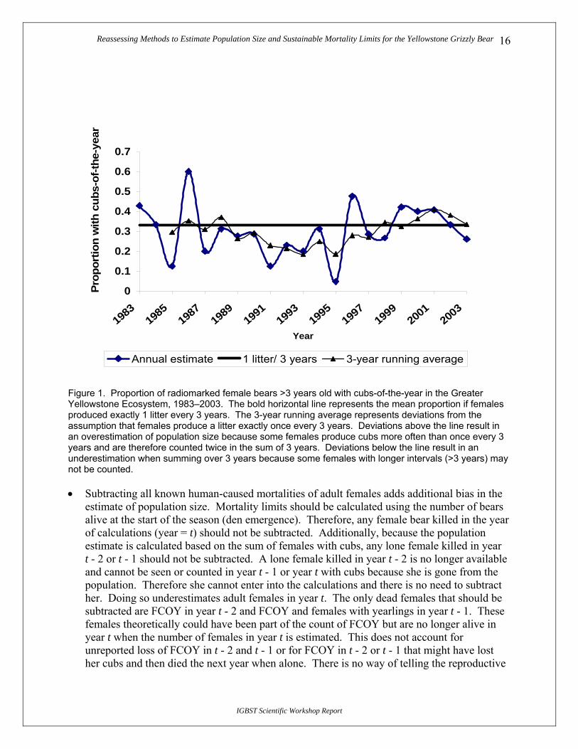
• It is assumed that on average, adult female grizzly bears produce a litter once every 3 years. Deviations from this assumption can overestimate (interval <3 years) or underestimate (interval >3 years) population size. The estimated proportion of FCOY in any given year based upon a sample of radiocollared bears (age >3) ranges from 0.05 to 0.60 (Fig. 1). The reciprocal of this value is the years between litters for this age group (i.e., 1/0.333 = 3). During this period (1983–2003), we monitored 352 females and documented 110 cub litters. This equates to 0.315 litters/female/year or 3.2 years between litters (1/0.315), suggesting that summing over 3 years creates a small underestimation of minimum population size.


0

0.1

0.2

0.3

0.4

0.5

0.6

0.7

1983

1985

1987

1989

1991

1993

1995

1997

1999

2001

2003

Year

Prop

ortio

n w

ith c

ubs-

of-th

e-ye

ar

Annual estimate 1 litter/ 3 years 3-year running average

Figure 1. Proportion of radiomarked female bears >3 years old with cubs-of-the-year in the Greater Yellowstone Ecosystem, 1983–2003. The bold horizontal line represents the mean proportion if females produced exactly 1 litter every 3 years. The 3-year running average represents deviations from the assumption that females produce a litter exactly once every 3 years. Deviations above the line result in an overestimation of population size because some females produce cubs more often than once every 3 years and are therefore counted twice in the sum of 3 years. Deviations below the line result in an underestimation when summing over 3 years because some females with longer intervals (>3 years) may not be counted.


• Subtracting all known human-caused mortalities of adult females adds additional bias in the estimate of population size. Mortality limits should be calculated using the number of bears alive at the start of the season (den emergence). Therefore, any female bear killed in the year of calculations (year = t) should not be subtracted. Additionally, because the population estimate is calculated based on the sum of females with cubs, any lone female killed in year t - 2 or t - 1 should not be subtracted. A lone female killed in year t - 2 is no longer available and cannot be seen or counted in year t - 1 or year t with cubs because she is gone from the population. Therefore she cannot enter into the calculations and there is no need to subtract her. Doing so underestimates adult females in year t. The only dead females that should be subtracted are FCOY in year t - 2 and FCOY and females with yearlings in year t - 1. These females theoretically could have been part of the count of FCOY but are no longer alive in year t when the number of females in year t is estimated. This does not account for unreported loss of FCOY in t - 2 and t - 1 or for FCOY in t - 2 or t - 1 that might have lost her cubs and then died the next year when alone. There is no way of telling the reproductive


history of a lone bear killed in year t. Consequently no matter how we attempt to “adjust” the 3-year sum to account for dead females no longer alive in year t, there is potential for error. Additionally, because the counts of FCOY only represent “observed” bears, subtracting a dead female likely reduces the sum of FCOY by removing females never observed and not part of the minimum count.

• Mortality limits were based on original work by Harris (1984) which was developed using input from a generic grizzly bear population for the continental U.S. These values may not remain valid for the GYE population, and more recent data are now available.

• Harris (1984) estimated maximum human-caused mortality limits of 6%. This level was reduced to 4% in the Recovery Plan to account for unknown unreported mortality. This was based on the assumption that for every 2 reported mortalities there was 1 additional unreported death. This ratio of 2:1 was an approximation that may no longer be appropriate for the GYE population today.

Group Discussion The group unanimously agreed that we have new peer reviewed scientific information (Cherry et al. 2002; Keating et al. 2002; Haroldson et al. 2005; Harris et al. 2005; Schwartz et al. 2005a, b, c) that can be used to improve existing methods, develop new methods for these management approaches, or both. The group agreed that we follow Dr. Gary White’s recommendation whenever feasible to “stay as close to the data as possible.” Because survival of independent females (age ≥2 years) was identified as the most important determinant of lambda (λ) with elasticity equal to 73% (Harris et al. 2005), we considered methods that allowed us to estimate independent female bears directly from the FCOY data.

WORKSHOP OBJECTIVES Once we decided to focus our efforts on developing a new method to set sustainable mortality limits for the GYE grizzly bear, we identified a number of components that needed to be considered in this process. Our objectives were to develop scientifically defensible methods to:

1. Refine methods to estimate total population size, adult female population size, and/or total female population size and address uncertainty.

2. Establish a biologically sustainable limit on total and female mortality. The group felt it necessary to explicitly define “biologically sustainable” so it was clear how we defined, established, and evaluated this important term.

3. Account for unknown and unreported mortality and if necessary, modify the 2:1 reported:unreported ratio based on empirical data.

4. Prepare a document that details this process and present our findings and recommendations to the Yellowstone Ecosystem Subcommittee for acceptance and approval.

ALTERNATIVE POPULATION ESTIMATION METHODS


Method 1.


Replace the number of unique females observed ( ) in Equation 1 above (see also Table 9) with one of the nonparametric estimators discussed by Keating et al. (2002). This is the method proposed in the Conservation Strategy (USFWS 2003) and should return an estimate of total population size given by the following equation:

iobsN ,ˆ

∑−=

−=

t

ti

ikeatingt

dNN

2 274.0

ˆˆ (2)

where is an estimate of total population size, and is one of the nonparametric estimators discussed by Keating et al. (2002).

tN̂ keatingN̂

Benefits • Provides an unbiased estimate of total FCOY, not just those observed. • Provides an annual estimate of uncertainty about FCOY. • Is unbiased by changes in observer effort. • Is a non-parametric estimator and thus avoids assumptions about form and constancy

of distribution of individual sighting probabilities. • approximates the total population rather than the minimum population size.

Consequently, mortality limits are a function of the total bear population. tN̂

Limitations • Application of to estimate FCOY assumes Knight et al. (1995) correctly

identifies individuals. keatingN̂

• Application of to estimate FCOY assumes clustering of sightings to be correct.

keatingN̂

• Variation among individual sighting probabilities (CV) affects performance of . It requires n/N ≥ 2, where n is the total number of sightings and N is the

population size. keatingN̂

• Replacing in the numerator of Equation (1) does not eliminate the other problems associated with it (i.e., assume 3-year breeding cycle, subtraction of all dead adult females, and the proportion of females in the population).

keatingN̂

Discussion Although the group felt that Equation 2 was an improvement over Equation 1 because of the value of the estimators, we concluded that we could develop alternative methods that would not only address switching from a minimum count to a total population estimate, but would also deal with other limitations of Equation 1. At this point our discussion shifted and we focused on estimators, their limitations, and recommendations for improvement.

keatingN̂

keatingN̂



Discussion of the Keating Estimator The group had considerable discussion about the application of the nonparametric estimators proposed by Keating et al. (2002). The bullets below capture that discussion. • In Keating et al. (2002), the modeled simulations only investigated CVs ≤ 1. The

estimate made from the empirical data collected in 2004 had an estimated CV = 1.1. Further, the estimator of CV used is known to be biased low. This exceeded the limits of the simulations, and the group recommended that Dr. Keating run additional simulations to investigate models with CV ≥ 1.0 and possibly up to 1.5.

• Also, in 2004, the population was estimated as = 72.6 (CV = 1.1) based on 202

sightings of 49 unique bears, where is the population estimate using the second-order sample coverage estimator. Contained in these sightings were observations from 7 individuals inside Yellowstone National Park where the sighting frequency was ≥10 sightings/individual. Chao et al. (1993, 2000) proposed an alternate method when some sighting frequencies were very common (suggesting that these individuals would be “known” to the population). We reapplied the estimator excluding these 101 sightings from these 7 unique bears. The estimate resulted in 51.9 unique bears, from 101 sightings; with these 7 females added back into the estimate as known individuals, the population estimate is 59 bears with estimated CV = 0.45.

SC2N̂

SC2N̂

• To illustrate how we might use information from the modeling, Dr. Keating used Figure 5b from Keating et al. (2002) (which shows the bias in CV) and extrapolated an estimated CV based on true CV = 1.1 and n/ = 2.8. He plugged that value into Figure 1 from Keating et al. (2002) considering n/N and estimated the original bias for the estimate of 72.6 to be about 20% too large. With this bias correction, the new estimate was = 58.

N̂

SC2N̂• After our discussions, it was decided that Dr. Keating would investigate the

following: o the Chao estimators relative to the possible removal of sighting of FCOY with

sighting frequencies n ≥ 10, or some other number o bias in estimates with CVs > 1.0 o a bias correction factor o using a model weighted approach or alternative methods under certain

circumstances (of those discussed by Keating et al. [2002]) o Use the initial Keating estimate of ( or a model weighted approach) to

refine the total females with cubs in the population. Attempt to minimize the root mean square error. Explore using estimator, which requires an initial estimate of population size, run the model, then take the resulting population estimate and put it back into the model and run it again until convergence.

SC2N̂ SC2N̂

SC2N̂

o Report results to the group at our second meeting.


• At our second workshop, Dr. Keating presented his results. During those discussions, we discovered that there was additional parameter space (distribution of sighting


probabilities) that had not been explored in the original Keating et al. (2002) simulations. Further investigation suggested that could be either positively or negatively biased depending on the probability distribution modeled. This prompted a reevaluation of the estimator. Further simulations confirmed the problem. Additional work based on simulation of sighting probabilities using a beta distribution with equal beta parameters and selecting from the extremes of the parameter space confirmed that can take either a positive or negative bias, and in some cases quite a large positive bias. On the other hand, it was also confirmed that the Chao

SC2N̂

SC2N̂

SC2N̂

2 estimator preformed well over the range of simulated population sizes and CVs ( = 20–80, CV = 0.0–1.75) and consistently returned estimates that were correct or biased low. Chao

N̂2 did a reasonable job when sighting probabilities were

high, but returned low estimates when probability sightings were quite small, likely because bears with extremely low sighting probabilities were not part of the “effective population size” from which the sample of sightings was actually drawn.

Method 2. Use as the best approximation of total FCOY in the population in any given year.

Estimate the annual proportion of FCOY ( ) in the adult female population from the telemetry sample (Table 9). The number of adult females in the population (≥4 years old) would be estimated as:

keatingN̂

FCOYP̂

FCOY

keatingfemales P

NN ˆ

ˆˆ = (3)


We looked at data from 1986 to 2002 and estimated . A graph of these values (Fig. 2) indicates large variation among annual estimates. Some of this noise is probably associated with poor estimates of the proportion of females with cubs from the telemetry sample due to small sample size and sampling bias (Table 9). But some noise may also be associated with the

estimator (i.e., 1995) when n/N < 1. All these issues affect the usefulness of this method.

femalesN̂

keatingN̂

Reassessing Methods to Estimate Population Size and Sustainable Mortality Limits for the Yellowstone Grizzly Bear


21

0100200300400500600700800900

1000

1985 1990 1995 2000 2005

Year

Num

ber

of F

emal

es

FCOYP̂

FCOYP̂

Figure 2. Estimated annual number of adult females in the Greater Yellowstone Ecosystem population based on the annual proportion of collared females ≥4 years old that produced cubs-of-the-year ( ) divided into the annual Chao2 estimator.

Limitations • depends on the telemetry sample, which in most years is small with a resulting

high variance component.

Benefits • Avoids the assumption that females produce cubs exactly once every 3 years. • Stays close to the real data. This method estimates females from empirical data. • Avoids the need to know the sex ratio of the population. • Avoids the need to subtract dead females. • Estimates the “total” number of females ≥4 years old. • The method could also be used to estimate number of independent females by

calculating the proportion of “independent females” (≥2 years old) in the telemetry sample, but estimates become more extreme in 1991 (345) and 1995 (1,427).

• Assumes the distribution of females in the telemetry sample is the same as the distribution in the population (i.e., we have the same proportion of 4-year-olds in the sample as in the population). This assumption may not be correct. To investigate this, we plotted the proportion of collared females by age in the telemetry sample against the modeled distribution (Harris et al. 2005) of females by age class using our best estimates of reproduction (Schwartz et al. 2005a) and survival (Haroldson et al. 2005, Schwartz et al. 2005b) (Figs. 3 and 4). Results suggest the age structure based on our best estimates of survival and reproduction differ from the age-structure of our captured sample. The proportion of females ages 2 and 3 are underrepresented, whereas females ages 6–8 appear overrepresented in the telemetry sample. The proportion of females in the telemetry sample with cubs-of-the-year was 0.267 and 0.311 for females ≥4 years old and ≥2 years old, respectively.

orking draft document on sustainable mortality limits for GYE grizzly bears 22 hwartz (9/2/2005).


Table 9. Number of observed unique unduplicated females (Nobs) with cubs-of-the-year (FCOY) based on the rule set of Knight et al. (1995), the estimated total number of unique FCOY ( ) based on the Chao2

ˆChaoN 2 estimator of Keating et al. (2002), the number of radiocollared females (age ≥4 years), and the

proportion ( ) and standard error (SE) of FCOY, estimated number of female bears age ≥4 or ≥2 year old, dependent young, and independent males. FCOYP̂

Population index

Female age

≥4 ≥2

Annual telemetry sample Dependent young

Year Nobs

2ˆ

ChaoN (n) ( FCOYP̂ a) (SEb)

2ˆ

ChaoN/ FCOYP̂

2ˆ

ChaoN / 0.248

( /0.289)/ 0.7734

2ˆ

ChaoN

2)]415.0(ˆ[ 2+femalesN 2)]}636.0)(ˆ[(ˆ{ 1,2,2 −+ tChaotChao NN Males age ≥2

1983 7 0.43 0.19 1984

6 0.33 0.19 1985 8 0.13 0.12 1986 25 27.5 15 0.60 0.13 46 111 123 102 74 1987 13 17.3 15 0.20 0.10 86 70 77 64 70 47 1988 19 21.2 16 0.31 0.12 68 85 95 79 64 57 1989 16 17.5 18 0.28 0.11 63 71 78 65 62 47 1990 25 25.0 14 0.29 0.12 86 101 112 93 72 68 1991 24 37.8 8 0.13 0.12 290 152 169 140 107 102 1992 25 40.5 13 0.23 0.12 176 163 181 150 129 110 1993 20 21.1 15 0.20 0.10 106 85 94 78 94 57 1994 20 22.5 16 0.31 0.12 73 91 101 84 72 61 1995 17 43.0 21 0.05 0.05 860 173 192 160 115 116 1996 33 37.5 21 0.48 0.11 78 151 168 139 130 102 1997 31 38.8 21 0.29 0.10 134 156 173 144 125 105 1998 35 36.9 15 0.27 0.11 137 149 165 137 123 100 1999 33 36.0 19 0.42 0.11 86 145 161 134 119 97 2000 37 51.0 30 0.40 0.09 128 206 228 189 148 138 2001 42 48.2 27 0.41 0.09 118 194 216 179 162 131 2002 52 58.1 24 0.33 0.10 176 234 260 216 178 157 2003 38 46.4 23 0.26 0.09 178 187 208 172 167 126 2004 49 57.5 232 257 214 174 156

a Calculated as the sum of telemetered bears observed over 3 years with cubs/total telemetered bears observed in the same 3-year period.

b Calculated as n

PP )1( −.

WPrepared by Chuck Sc

23

0

0.02

0.04

0.06

0.08

0.1

0.12

0.14

4 5 6 7 8 9 10 11 12 13 14 15 16 17 18 19 20 21 22 23 24 25 26 27 28 29 30

Age in Years

Prop

ortio

n proportion in sample

proportion in population

Figure 3. The proportion of female bears ≥4 years old in the telemetry sample (1983–2001) in the Greater Yellowstone Ecosystem and the proportion of these age classes in the population based on simulation modeling using empirical data on reproduction and survival (Appendix A).

0

0.02

0.04

0.06

0.08

0.1

0.12

0.14

2 4 6 8 10 12 14 16 18 20 22 24 26 28 30

Age in Years

Prop

ortio

n

proportion in sample

proportion in population

Figure 4. The proportion of female bears ≥2 years old in the telemetry sample (1983–2001) in the Greater Yellowstone Ecosystem and the proportion of these age classes in the population based on simulation modeling using empirical data on reproduction and survival (Appendix A).

Discussion


Dr. White presented information on transition rates among various states for female bears ≥4 year old (Appendix C). These transitions are unbiased relative to sampling and would help resolve the telemetry sample bias problem discussed above. His results suggest that we tend to capture more bears in the “N” state (no offspring) than those in the “C”, “Y”, or “T” states (with cubs, yearlings, or 2-year-olds). Consequently, the proportion of females with cubs in the telemetry sample appears biased low. Based on these discussions, we concluded we should not recommend using the telemetry sample to estimate the proportion of FCOY in any given year as the denominator of Equation 3.

24

We also looked at the SEs of the proportion of females with cubs in the telemetry sample (Table 9) and concluded that nearly all annual estimates were not statistically different, suggesting we could use a constant in the denominator.

Method 3. Use the logic described in Method 2 above, but base estimates on a 3-year (or even a 6-year) running average of and (Table 9). keatingN̂ FCOYP̂

Benefits • Running average dampens the noise in the estimate. • Running average increases sample size.

Limitations • Still assumes the distribution of females in the telemetry sample is the same as

the distribution in the population. • Running average is influenced by the number of years in the average. If we

use a 6-year average, the variance is dampened even more than with a 3-year average. However, for a declining population, the average estimate will be greater than the true population (i.e., the previous 5 years elevate the mean). This works in reverse for a growing population and becomes equivocal for a flat trajectory. Hence the running average is conservative for a growing population but may result in over-harvest for a declining population. Alternatively, we could consider a 6-year average for a growing population but recommend it be shortened to a 3-year average should trends suggest the population is declining.

Discussion We rejected this approach for reasons discussed under Method 2. We also had a long discussion on assumptions and issues associated with using a “running average” to smooth data. The group felt uncomfortable with such an approach because of possible unknown statistical biases.

Method 4. Use an estimate of the proportion of females with cubs (age ≥4 years or ≥2 years) relative to an estimate of total “adult” or “independent” females in the GYE population. For example, Harris (Appendix A) estimated the proportion of females ≥2 years old accompanied by cubs based upon stochastic simulation modeling was 0.248 of all females ≥2 years of age in the GYE population. Using this value, we estimate total independent females in the GYE population with the following equation:

248.0

ˆˆ keating

females

NN = (4)


where ( ) is the number of FCOY based on one of the estimators reviewed by

Keating et al. (2002), and is an estimate of females age ≥2 years old in the population. Harris (Appendix A) estimated that on average over a 10-year simulation,

keatingN̂

femalesN̂

25

FCOY in the population constitute 0.247 (CV = 0.110) and 0.248 (CV = 0.105) of the female population ≥2 years of age when adult female survival is set at 0.949 or 0.922, respectively. He also calculated the number of females in the population age ≥4 years old as 0.314 and 0.315 (adult female survival = 0.922 or 0.948).

Benefits • Simple to calculate. • Avoids bias associated with the sample of collared females. • Based on empirical data.

Limitations • Constant in the denominator does not allow for temporal changes in

reproductive rates. • Constant in the denominator requires periodic updates.

Discussion The group felt this was the best method. We had considerable discussion on what value to use for the denominator. Dr. White offered an alternative for estimating total number of females ≥4 years of age in the population. He used the telemetry dataset and determined the proportion of females (age ≥4) in the population with cubs-of-the-year in this sample using a multi-state model (results are in Appendix C). His estimate (0.289) was quite similar to the Harris estimate of 0.314 (Appendix A) based on modeling. Because Dr. White’s estimate was based on empirical data, we chose to use it.

We discussed the value of developing an index of the female population ≥4 years of age using the constant 0.289 directly. Because analyses by Haroldson et al. (2005) found no statistical or biological difference in survival for independent subadult (ages 2–4 years) and adult (ages ≥5 years) bears, we concluded that it would be simpler to derive a single population estimate of independent females. Using data from Harris et al. (2005), we estimated the proportion of females ≥4 years and older in the population of females ≥2 years old (Tables 10 and 11). Because Harris et al. (2005) estimated the stable age distribution using both high and low survival estimates for independent females (0.92 and 0.95) which considered both high and low process variance, we evaluated both and the magnitude of difference between the 2 estimates. Results (Tables 10 and 11) indicated that there was virtually no difference in the proportional estimates when using the low or high survival rate for independent females (0.773421 vs. 0.773392). Consequently, we used 0.7734 as the proportion of females ≥4 years old in the population of independent females ≥2 years old. We used this to convert our estimate with the following equation:

)7734.0*289.0(

ˆˆ 2

2Chao

femalesN

N =+ (5)


where ( ) is the number of FCOY based upon the Chao2 estimator, and 0.289 is the proportion of females ≥4 years of age accompanied by cubs-of-the-

2ˆ

ChaoN

26


year (Appendix C) in the telemetry sample, and 0.7734 is the proportion of female bears ≥4 years of age in the standing population of females ≥2 years of age.

27

Table 10. Deterministic projections of stable age structure of the Greater Yellowstone Ecosystem grizzly bear population. Data from Harris et al. (2005:Table 18) and lx = survivorship schedule.

Adult female survival = 0.92 Adult male survival = 0.823

Age years lx

Stable age distribution

Proportion by years 0–30 lx


Proportion by years 0–30

0 1.000 1.000 0.1831 1.000 1.000 0.2624 1 0.630 0.605 0.1107 0.630 0.605 0.1587 2 0.504 0.464 0.0850 0.504 0.464 0.1218 3 0.464 0.410 0.0750 0.415 0.367 0.0962 4 0.427 0.362 0.0662 0.341 0.290 0.0760 5 0.392 0.319 0.0585 0.281 0.229 0.0600 6 0.361 0.282 0.0516 0.231 0.181 0.0474 7 0.332 0.249 0.0456 0.190 0.143 0.0374 8 0.306 0.220 0.0403 0.157 0.113 0.0296 9 0.281 0.194 0.0355 0.129 0.089 0.0234 10 0.259 0.171 0.0314 0.106 0.070 0.0184 11 0.238 0.151 0.0277 0.087 0.056 0.0146 12 0.219 0.134 0.0245 0.072 0.044 0.0115 13 0.201 0.118 0.0216 0.059 0.035 0.0091 14 0.185 0.104 0.0191 0.049 0.027 0.0072 15 0.170 0.092 0.0168 0.040 0.022 0.0057 16 0.157 0.081 0.0149 0.033 0.017 0.0045 17 0.144 0.072 0.0131 0.027 0.013 0.0035 18 0.133 0.063 0.0116 0.022 0.011 0.0028 19 0.122 0.056 0.0102 0.018 0.008 0.0022 20 0.112 0.049 0.0090 0.015 0.007 0.0017 21 0.103 0.044 0.0080 0.012 0.005 0.0014 22 0.095 0.038 0.0070 0.010 0.004 0.0011 23 0.087 0.034 0.0062 0.008 0.003 0.0009 24 0.080 0.030 0.0055 0.007 0.003 0.0007 25 0.074 0.026 0.0048 0.006 0.002 0.0005 26 0.068 0.023 0.0043 0.005 0.002 0.0004 27 0.063 0.021 0.0038 0.004 0.001 0.0003 28 0.058 0.018 0.0033 0.003 0.001 0.0003 29 0.053 0.016 0.0029 0.003 0.001 0.0002 30 0.049 0.014 0.0026 0.002 0.001 0.0002

Proportion of the population ≥4 years of age 0.5462 Proportion of the population ≥2 years of age 0.7062 Proportion of females ≥4 years of age of females ≥2 years of age 0.773421 Proportion of the population ≤1 years of age 0.294 Proportion of females ≤1 years of age of females ≥2 years of age 0.416 Male:female ratio (age≥2) 0.3638:0.6362


28

Table 11. Deterministic projections of stable age structure of the Greater Yellowstone Ecosystem grizzly bear population. Data from Harris et al. (2005:Table 18) and lx = survivorship schedule.

Adult female survival = 0.95 Adult male survival = 0.874

Age years lx


Proportion by years 0–30 lx


Proportion by years 0–30

0 1.000 1.000 0.1826 1.000 1.000 0.2451 1 0.650 0.604 0.1103 0.650 0.604 0.1481 2 0.540 0.466 0.0851 0.540 0.466 0.1142 3 0.513 0.411 0.0751 0.472 0.379 0.0928 4 0.487 0.363 0.0663 0.412 0.307 0.0753 5 0.463 0.321 0.0586 0.360 0.250 0.0612 6 0.439 0.283 0.0517 0.315 0.203 0.0497 7 0.417 0.250 0.0457 0.275 0.165 0.0404 8 0.397 0.221 0.0403 0.240 0.134 0.0328 9 0.377 0.195 0.0356 0.210 0.109 0.0266 10 0.358 0.172 0.0314 0.184 0.088 0.0216 11 0.340 0.152 0.0277 0.161 0.072 0.0176 12 0.323 0.134 0.0245 0.140 0.058 0.0143 13 0.307 0.118 0.0216 0.123 0.047 0.0116 14 0.292 0.105 0.0191 0.107 0.038 0.0094 15 0.277 0.092 0.0169 0.094 0.031 0.0077 16 0.263 0.081 0.0149 0.082 0.025 0.0062 17 0.250 0.072 0.0131 0.072 0.021 0.0050 18 0.237 0.064 0.0116 0.063 0.017 0.0041 19 0.226 0.056 0.0102 0.055 0.014 0.0033 20 0.214 0.050 0.0090 0.048 0.011 0.0027 21 0.204 0.044 0.0080 0.042 0.009 0.0022 22 0.193 0.039 0.0070 0.036 0.007 0.0018 23 0.184 0.034 0.0062 0.032 0.006 0.0014 24 0.175 0.030 0.0055 0.028 0.005 0.0012 25 0.166 0.027 0.0049 0.024 0.004 0.0010 26 0.158 0.023 0.0043 0.021 0.003 0.0008 27 0.150 0.021 0.0038 0.019 0.003 0.0006 28 0.142 0.018 0.0033 0.016 0.002 0.0005 29 0.135 0.016 0.0029 0.014 0.002 0.0004 30 0.128 0.014 0.0026 0.012 0.001 0.0003

Proportion of the population ≥4 years of age 0.547 Proportion of the population ≥2 years of age 0.707 Proportion of females ≥4 years of age of females ≥2 years of age 0.773392 Proportion of the population ≤1 years of age 0.293 Proportion of females ≤1 years of age of females ≥2 years of age 0.414 Male:female ratio (age ≥2) 0.3901:0.6099


29

Our annual index of population size for females ≥2 years of age is then = . The denominator of 0.224 is not statistically different from the estimate of Harris (Appendix A) of 0.248.

+2ˆ

femalesN

We also discussed the variation in our annual estimates and how we might dampen this variation to reduce the wide swings in allowable mortality limits based on this population index. We considered using a 3-year running average of

to dampen variation, but the group felt there were potential statistical problems with any such calculations. Consequently, we elected to generate an annual population size of independent females ≥2 years of age and use that estimate to establish an annual mortality quota.

+2ˆ

femalesN

Finally, we discussed the stable age structure and the appropriate number of age classes to consider. In their modeling, Harris et al. (2005) used 31 age classes. We evaluated this number relative to known longevity of bears and concluded it was probably quite close to the maximum life expectancy of bears in the GYE. We came to this conclusion based on the following: Justification for using 31 Age Classes (Ages 0–30) The IGBST documented 19 individual grizzly bears living ≥20 years in the GYE during 1975–2004. Twelve of these were known to have died, while the fates of an additional 7 were unknown (Table 12).

Table 12. Fate of radiocollared grizzly bears in the Greater Yellowstone Ecosystem, ≥20 years of age, 1975–2004.

Last known fate Age Alive Dead Total 20 2 3 5 21 1 3 4 22 2 3 5 24 1 1 2 25 1 1 2 28 0 1 1

Total 7 12 19 The oldest bears documented in the GYE were 25 and 28 for females and males, respectively (Table 13). The oldest female known to have produced cubs was 25. We currently (2005) have a 25-year-old female radiomarked.


Table 13. Age and sex of oldest known grizzly bears in the Greater Yellowstone Ecosystem, 1975–2004.

Sex Age Female Male Total 20 3 2 5 21 2 2 4 22 2 3 5 24 1 1 2

30

25 1 1 2 28 0 1 1

Total 9 10 19

Estimating Numbers of Cubs, Yearlings, and Independent Males: Because our index of abundance only addressed independent females, we explored additional ways to estimate abundance of cubs, yearlings, and male bears. We elected to treat cubs and yearlings as a group because dependent young are exposed to different mortality causes, and if there is ever a hunting season, cubs and yearlings would be protected. Keeping them separate from any quota of independent female and male bears facilitates managing a hunt. We explored 2 alternative methods to estimate the cubs and yearlings in the population:

1. The first was based on the stable age distribution (Tables 10 and 11). We determined that for every female ≥2 years of age, there were 0.414 or 0.416 dependent females (cubs and yearlings), using low and high survival rates of adult females. We used the mean value (0.415) to estimate numbers of dependent females in the population by multiplying our estimate of

from Equation 5 by 0.415 +2ˆ

femalesN

2)]415.0(ˆ[ˆ2+= femalesyoungdependent NN (6)

Finally, we chose to consider both sexes of cubs and yearlings together so we multiplied our estimate of dependent female bears by 2 to estimate the total number of dependent offspring in the population ( ). youngdependentN̂

2. We assumed average litter size was 2 cubs (Schwartz et al. 2005a estimated mean litter size = 2.04), with a 50:50 sex ratio. We also assumed cub survival = 0.638 (Schwartz et al. 2005b). We calculated the number of cubs and yearlings in the population using the following equation:

2)]}638.0)(ˆ[(ˆ{ˆ1,2,2 −+= tChaotChaoyoungdependent NNN (7)

where is an annual estimate of dependent offspring,

number of FCOY in year t, and is the number of females with cubs in year t - 1.

youngdependentN̂ t Chao2,N̂

1-t Chao2,N̂

Results using this method yield fewer cubs and yearlings on average than Method 1. We used this method because the number of dependent young is calculated directly from field data.


3. We estimated the number of males directly from our estimate of independent females. Based on simulation modeling, Harris et al. (2005) estimated that the ratio of male:female bears ≥2 years old in the GYE population was

31

0.377:0.623. This effectively means that for each female in the population, there are 0.605 males (0.377/0.623 = 0.605). We calculated the number of independent males using the following equation (Table 9):

)605.0(ˆˆ22 ++ = femalesmales NN (8)

Area of inference During our second workshop we discussed the area of inference and application of our estimators to segments of the GYE population. The population estimators reviewed by Keating et al. (2002) are for closed populations. We concluded that our estimates are appropriate at the GYE population level. As a consequence, our estimates of sustainable mortality are also appropriate at the population level.

SUSTAINABLE MORTALITY LIMITS

To address objective 2 we considered the current method and evaluated and discussed other options.

Current Method To facilitate recovery and to account for unknown, unreported, human-caused mortality, known human-caused mortality was set by the USFWS Grizzly Bear Recovery Plan at 4% of the minimum population estimate (USFWS 1993). Female mortality was set at 30% of this 4% limit. Limits of acceptable mortality were derived from Harris (1986) using a model of a generic bear population in the Rocky Mountains. Harris (1986) suggested that grizzly bear populations could sustain approximately 6% human-caused mortality without population decline. The difference between the 4% in the Recovery Plan and 6% of Harris (1986) allowed for an unreported loss of 2% from human causes.

Benefits • Under the current mortality limits, the GYE population has increased at an

average rate of between 4–7% per year. It appears conservative (at least when coupled with the minimum population estimate).

• It can be applied to any of the proposed population methods discussed above.

Limitations • Estimates are based on generic grizzly bear population, not specific to the

GYE. • More updated and detailed information is available to model the population. • Method assumed an unstated reporting rate of 2:1 (reported:unreported),

which is inconsistent with current estimates for GYE grizzly bears.

Discussion


We discussed several issues. The current method only considers known and probable human-caused mortality. The 6% limit does not consider undetermined or natural mortality. This is an issue when cause of death is reported as “undetermined” because these deaths are not counted against the threshold.

32

However, it is likely that many of these mortalities were in fact human-caused deaths. The 6% limit was reduced to 4% to account for an unknown and unreported mortality of 2%. This can be interpreted as 1 unreported loss for every 2 known losses. However, Knight and Eberhardt (1985:330) stated that actual mortality in the GYE “appears to be approximately double that recorded.” This result is consistent with current estimates of reporting rate (Appendix B). The recent analysis by Harris et al. (2005) suggests that the 6% sustainable mortality limit is very conservative and can be increased. The group decided to explore alternate methods of establishing mortality limits using all of the most recent information published by Cherry et al. (2002), Harris et al. (2005), Haroldson et al. (2005), and Schwartz et al. (2005a, b).

ALTERNATIVE MORTALITY THRESHOLDS

Independent Females ≥2 Years Old Adjust sustainable mortality limits to match what is required to maintain λ ≥ 1 based on more recent simulation models by Harris et al. (2005). The GYE grizzly bear population is likely to maintain a positive trajectory as long as survival of independent females (aged ≥2 years) remains above approximately 0.91 (i.e., 9% annual mortality from all causes).

Benefits


• This would bring the limits in line with empirical data from the GYE as discussed by Schwartz et al. (2005c). Additionally, Harris et al. (2005) indicated regarding this 9% mortality that: It would seem, at first blush, to suggest a radical departure from current guidelines. For example, Harris (1986:273) recommended that ‘the proportion of the female segment of the population that can be removed annually…without causing chronic decline should not exceed 3% of the female segment.’ More recently, McLoughlin (2002:33) suggested that ‘most grizzly bear populations in North America can tolerate approximately 3% total annual kill before declines…accelerate to unsatisfactory levels.’ Careful reading, however, reveals that, beyond some minor differences in assumptions and procedures, the apparent increase in tolerable mortality we report here arises not from real discrepancies in models or parameter values but rather from different ways of expressing a similar underlying dynamic.

Comparing our results with those of Harris (1986) is important because current management guidelines in the Yellowstone Grizzly Bear Recovery Zone (USFWS 1993, 2003) adopt an annual mortality limit derived largely from that work. First, our approach here differed fundamentally in that the earlier work attempted to estimate the mortality level associated with sustainability indefinitely. That is, Harris (1986) used a model of grizzly bear population dynamics that was self-regulating. Thus, bear populations in

33


Harris (1986) equilibrated (rather than growing exponentially) in the absence of killing by humans. Adding human-caused deaths to this model engaged compensatory responses that were assumed to characterize grizzly bear populations (although parameters used to build the responses were not based directly on data, but rather were interpolated from general principles). Here, our aims were more modest: to project short-term growth rates applied under a range of plausible survival rates, making no assumptions about density-dependent (or other possible) regulating mechanisms that would, no doubt, intercede to change those trajectories. Second, Harris (1986) assumed that natural mortalities, although decreasing as hunting increased, would never be entirely substituted by human-caused mortality. That is, even at the population level producing the highest sustainable yield indefinitely, background levels of natural mortality would continue. Harris’ (1986) objective was to estimate the maximum human-caused mortality rate that, when embedded into the assumed compensatory structure, equilibrated the population with its carrying capacity. Here, we declined to suppose any particular relationship between human- and nonhuman-caused mortalities (to say nothing of carrying capacity). Indeed, we had no data to do otherwise, given that not a single independent female mortality in GYE attributable to non-human causes was documented during 1983–2001 (Haroldson et al. 2005). Dependent young experienced natural mortality, but because cubs and yearlings were not collared, cause of death was undetermined in many cases (Schwartz et al. 2005b). Thus, contrasting our results directly with the 3% sustainable mortality rate of females estimated by Harris (1986) is inappropriate. Harris (1986) also assigned survival rates to 3 subadult female classes (ages 2, 3, and 4 years) in addition to 3 adult age classes, complicating any attempt to compare the total mortality rate sustained by adult females in his model populations with those we report here. Fortunately, we were able to rehabilitate the Harris (1986) model for application here and develop a common currency for comparison with results reported here. We discovered that maximum hunting rates he found consistent with sustainability (i.e., 6.85 female kills/year from a population of 193.5 females, or 3.54% of the female component killed annually; Harris 1986:276) corresponded to an annual survival rate of all females (cubs through the oldest class) of 0.851 (SD = 0.035, n = 3,000). For comparison, our survival rates of all females (irrespective of age) consistent with low probability of decline were 0.847 (SD = 0.022, n = 3,000) when independent female survival was 0.91 (under low process variation) and 0.852 (SD = 0.077, n = 6,000) when independent female survival was 0.92 (under high process variation). Thus, although the approaches and presentation of results were quite divergent, overall female survival rates consistent with nondeclining populations in both Harris (1986) and our present effort were almost identical.

34

McLoughlin (2002) reported that a simulated population modeled approximately on GYE grizzly bear data through 1995 displayed a breakpoint (at which persistence probability declined rapidly with additional kills) at a mortality rate of about 2.8%. However, human-caused mortalities in his model were assumed additive to natural mortality, which was set at 4.9% for females aged ≥6 years and 11.4% for females aged 2–5 years (McLoughlin 2002:Table 2.1). With approximately 30% of the female population in ages 2–5 years and 46% ≥6 years old (approximately the case if the population had achieved its stable age distribution prior to additional harvest), the mean natural mortality rate for females ≥2 years would thus be approximately 6.4%. This, added to the 2.8% annual kill, yields 9.2% total mortality of females age ≥2 years (i.e., annual survival of 0.908), which is again similar to our conclusion that λ will be ≥1 with high probability when annual female (age ≥2 years) survival rates were approximately 0.90–0.91. Eberhardt (1990) also provided a simple deterministic model relating grizzly bear life history rates to stable trajectories. Application of the mean survival rates from our simulations to (Eberhardt 1990:587) produced r = 0 (i.e., λ = 1.0) with independent female (≥2 years old) survival of 0.898 and age of first reproduction set to 5 years, as well with as with independent female survival of 0.906 and age of first reproduction set to 6 years (GYE mean during 1983–2002 was 5.81 years, but Eberhardt’s [1990] equation did not allow for fractional ages). Although abstract, his model further confirmed our estimates of female survival rates consistent with nondeclining trajectories. The current approach to grizzly bear management in GYE is for management agencies to consider all forms of mortality, but to establish an annual mortality limit only for human-caused mortality. We propose that rather than counting human-caused mortalities, management agencies should focus on female survival rates irrespective of the cause of death. By counting all deaths, it becomes unnecessary to determine exactly how a bear died (which often requires subjective judgments). It also minimizes the importance of knowing the proportion of human-caused deaths not documented (e.g., Cherry et al. 2002). As long as an active monitoring program is in place (including radiotelemetry of a random sample of bears to update life-history rates as conditions change), demographic analyses can augment counts of reproductively-active females (Knight et al. 1995, Mattson 1997, Keating et al. 2002) as an indicator of overall population health.

• This limit is based on survival estimates for females ≥2 years of age. It will allow us to set limits for independent females using methods discussed above to estimate independent females in the population.

• Allows for separate limits for male bears.

Limitations


• This is a total mortality limit for independent female bears. It includes both natural and human-caused deaths. We were unable to estimate the rate of

35

“natural mortality” for independent female bears because we did not document any natural mortality in the telemetry sample of females from 1983–2002. This must be considered when using this method.

• The limit only addressed independent females and requires we consider dependent young separately.

• Requires we establish limits for males separately or establish a geographically-based limit system.

Discussion The group felt it was essential to distinguish between a mortality limit that is not to be exceeded and a mortality target that is a management objective. Consequently, we defined a sustainable mortality limit for female grizzly bears (≥2 years of age) in the GYE as the maximum allowable mortality that the female population can sustain over time and maintain population stability (stability is defined as λ =1.0) with a 95% level of confidence. Based on Harris et al. (2005), if we set independent female survival = 0.89, the point estimate of λ = 1.005 with a 95% confidence interval 0.97–1.04. Because this estimate overlaps 1.0, and there is a chance that when survival = 0.89, λ < 1, we recommended the following:

i. Use a survival rate of 0.91 (λ = 1.03, CI 1.0–1.05), which allows for increased confidence that λ ≥ 1.0. We did this because the estimate accounts for process variation inherent in annual female survival in the GYE.

ii. The States of Wyoming, Montana, and Idaho set the near-term objective for the GYE bear population to continue expanding into suitable habitat. To assure population health with an acceptable level of risk, we chose a point estimate of survival for females that has the lower 95% CI of λ = 1.0.


We also discussed mortalities to include for tabulation of total independent female mortality. The group recommended we consider all forms of mortality, including human-caused, natural, and undetermined, against the quota. This eliminated the need to determine cause of death, eliminated the possibility of misclassification, and stays closer to our estimate of 9% total mortality from all causes. Natural mortality appears quite low for independent females in the GYE. Results presented by Haroldson et al. (2005) indicated no recorded natural deaths for independent female bears based on telemetry from 1983–2001 from a sample of 3,420 radio-months (285 bear-years). We determined the binomial confidence bounds for these data with x = 0, n = 285, where p = x/n using the formula: 0≤ p ≤ 1- α1/n (van Belle 2002). At α = 0.05 and n = 285, the upper bound of the confidence interval = 0.0105. This suggests that although we did not document natural mortalities over the 19-year-period with a sample of 285 bear-years, there was a small chance we missed one. Regardless, the data suggest that natural mortalities are rare and would not contribute much to the total mortality limit whether included or excluded in the tally. Consequently, we elected to count all forms of mortality for independent female bears.

36


Results of these calculation and thresholds are shown in Table 14.

Dependent Offspring (Cubs And Yearlings)

We discussed the establishment of a limit on mortality for cubs and yearlings. 1. Because we often lack information on the sex of dead cubs and yearlings, we elected

to establish a limit for both sexes. Although survival estimates for cubs-of-the-year (0.638) and yearlings (0.817) were lower than survival of independent bears, we elected to set the mortality limit the same for the following reasons: • Only human-caused mortalities would be counted. We decided this because

numbers of recorded cub and yearling mortalities are linked to the number of adult female bears collared. Most of the documented deaths of offspring of collared bears are of undetermined cause. Data presented by Schwartz et al. (2005b) suggests these are likely natural deaths. We cannot limit natural deaths but need to consider human-caused mortality and ensure it does not exceed sustainability. From the sample of dependent young, 10 of 32 cubs, and 1 of 5 yearlings died from human related causes. This equated to 11 of 37 (0.297) mortalities recorded as human-caused, or about 30% of recorded mortality was human-caused.

The method of Cherry et al. (2002) to estimate unknown and unreported mortalities is based on reporting rate from a sample of telemetry bears. Dependent young were not radiomarked. We therefore elected to count only known and probable human-caused deaths for dependent young and set the limit at 9% for both sexes. We will assume reporting rates for dependent young are similar to reporting rates of independent bears (which is likely because most dependent young, especially cubs, die if their mother dies). Reporting rates for independent bears are roughly 1 reported for 2 unreported. The 9% reported limit is then roughly equivalent to a 27% total mortality rate (9% reported:18% unreported). Total mortality from birth to recruitment as a 2-year-old is 0.48 (1 - [0.638 x 0.817]). Assuming human-caused mortality remains about the same, one would expect about 14.3% of this recorded mortality to be human caused (0.48 x 0.297 = 0.143). Accounting for both sexes, this equates to about 28.6% mortality (0.143 x 2 = 0.286), which approximates the proportion of recorded human-caused mortality rates from 1983–2001 (0.297).

• We also discussed the implications of error in our estimates. A 9% limit is conservative for dependent young. Secondly, survival of dependent young only contributed 17.8% to the elasticity of lambda calculations (Harris et al. 2005)

Alternatively, we estimated from transition probabilities (Appendix C) that approximately 0.529 females ≥4 years of age were accompanied by either cubs or yearlings in any given year. A simpler approach would set a limit that no more than half of all females ≥4 years old tallied in the mortality quota could be accompanied by cubs or yearlings. We did not choose this alternative because it does not allow for consideration of dependent young that die independently of their mothers.

37


Table 14. Estimated number of females with cubs-of-the-year ( ) and independent females aged ≥2 years old in the Greater Yellowstone Ecosystem, 1986–2004. Mortalities were listed by cause (management removal [MGMT], known because of telemetry [TELE], reported by the public [PUBL], estimates of known, unknown, and unreported [KNO:UNR), and total. The annual mortality limit from all causes was set at 9% of the annual female estimate. The 3-year running average of mortality smoothed the limit and was used as a threshold. Status indicates if threshold was exceeded and the probability of exceeding the threshold based on the credible interval used to calculate unknown and unreported mortality.

2ˆ

ChaoN

Female mortality

Year 2ˆ

ChaoN Females ≥2 years MGMT TELE PUBL

KNO:UNRa Total

9% mortality

limit

3-year running average

limit Status P̂ of

exceedingb

1986 27.5 123 1 3 1 2 6 11 1987 17.3 77 1 0 1 2 3 7 1988 21.2 95 0 1 0 1 2 9 9 OK 0.003 1989 17.5 78 0 0 0 1 1 7 8 OK 0.003 1990 25.0 112 1 2 3 7 10 10 9 exceeded 0.484 1991 37.8 169 0 0 0 1 1 15 11 OK 0.000 1992 40.5 181 0 1 0 1 2 16 14 OK 0.000 1993 21.1 94 0 1 2 5 6 9 13 OK 0.031 1994 22.5 101 0 2 1 2 4 9 11 OK 0.014 1995 43.0 192 3 0 3 7 10 17 12 OK 0.235 1996 37.5 168 1 3 2 5 9 15 14 OK 0.059 1997 38.8 173 0 0 3 7 7 16 16 OK 0.036 1998 36.9 165 0 0 1 2 2 15 15 OK 0.002 1999 36.0 161 0 0 1 2 2 14 15 OK 0.002 2000 51.0 228 1 1 3 7 9 21 17 OK 0.047 2001 48.2 216 5 3 1 2 10 19 18 OK 0.010 2002 58.1 260 2 2 4 10 14 23 21 OK 0.079 2003 46.4 208 1 0 5 13 14 19 20 OK 0.115 2004 57.5 257 4 0 5 13 17 23 22 OK 0.142 aData in this column are estimates of unknown and unreported mortality plus mortalities reported by the public. The method of Cherry et al. (2002) estimates the number of times an event occurred given an observed outcome and the probability of that outcome. For example, the method would estimate the number of times a coin was flipped given that 3 heads were observed and the probability of a heads was 0.5. In our case here, it estimates the number of dead bears (both reported and unreported) given the number reported by the public. So in 2004,

38


given that 5 bears were reported dead, the method estimated that 13 actually died bThe probability of exceeding was based on the method of Cherry et al. (2002). The probability values represent the likelihood of exceeding the 3-year running limit minus the known deaths (MGMT and TELE), given a public reporting (PUBL) rate for that year. For example in 2004, the 3-year limit was 22. The probability is therefore the likelihood of exceeding 19 deaths (22 – 4 - 0 +1 = 19) given that 5 were reported.

39


Independent Males ≥2 Years Old We used empirical data to establish a male mortality limit based on estimates from 1983–2001 (Haroldson et al. 2005). Estimated survival of independent male bears in the GYE equaled either 0.874 or 0.823 for the censored and assumed dead data sets. We split the difference and established the limit of mortality equal to 0.15. Results of calculations and thresholds are reported in Table 15. Male limits are based on the status quo and the past 20 years, when the GYE grizzly bear population increased in size and expanded in range.

UNKNOWN AND UNREPORTED MORTALITY

To address objective 3, we considered the current method and evaluated and discussed other options.

Current Method • Harris (1986) suggested that grizzly bear populations could sustain

approximately 6% human-caused mortality without population decline. To facilitate recovery and to account for unknown, unreported, human-caused mortality, known human-caused mortality was set by the USFWS Grizzly Bear Recovery Plan at 4% of the minimum population estimate (USFWS 1993). The reduction from 6% to 4% was justified because an assumption was made that for 2 reported mortalities, an additional one was unreported.

However, Knight and Eberhardt (1985:330) stated that actual mortality in the GYE “appears to be approximately double that recorded.”

Benefits • Simple. • Can be applied to any of the proposed population methods above. • Has worked in the past.

Limitations • Does not include estimates of uncertainty. • This ratio may have changed.

Discussion We all agreed that there was better information and that we should explore new methods to account for unknown and unreported mortality.

40


Table 15. Estimated number of females with cubs-of-the-year ( ) and independent males (≥2 years old) in the Greater Yellowstone Ecosystem, 1986–2004. Mortalities were listed by cause (management removal [MGMT], known because of telemetry [TELE], reported by the public [PUBL], estimates of known, unknown, and unreported [KNO:UNR), and total. The annual mortality limit from all causes for males ≥2 years old was set at 15% of the male population estimate. The 3-year running average of mortality smoothed the limit and was used as a threshold. Status indicates if threshold was exceeded, and the probability of exceeding it was provided based on the credible interval used to calculate unknown and unreported mortality.

2ˆ

ChaoN

Male mortality

Year 2ˆ

ChaoN

Males ≥2

years MGMT TELE PUBL UNK:UNR Total

15% mortality

limit

3-year running average

limit Status P̂ of

exceeding 1986 27.5 74 1 1 0 1 3 11 1987 17.3 47 2 1 0 1 4 7 1988 21.2 57 1 1 1 2 4 9 9 OK 0.031 1989 17.5 47 1 1 1 2 4 7 8 OK 0.046 1990 25.0 68 1 1 2 5 7 10 9 OK 0.154 1991 37.8 102 0 0 0 1 1 15 11 OK 0.000 1992 40.5 110 2 5 1 2 9 16 14 OK 0.031 1993 21.1 57 0 2 0 1 3 9 13 OK 0.000 1994 22.5 61 0 1 1 2 3 9 11 OK 0.010 1995 43.0 116 2 4 4 10 16 17 12 exceeded 0.750 1996 37.5 102 2 2 3 7 11 15 14 OK 0.182 1997 38.8 105 1 1 2 5 7 16 16 OK 0.016 1998 36.9 100 2 2 0 1 5 15 15 OK 0.000 1999 36.0 97 2 2 3 7 11 15 15 OK 0.140 2000 51.0 138 2 4 11 29 35 21 17 exceeded 1.000 2001 48.2 131 7 2 1 2 11 20 18 OK 0.014 2002 58.1 157 4 1 3 7 12 24 21 OK 0.036 2003 46.4 126 2 3 3 7 12 19 21 OK 0.036 2004 57.5 156 3 2 7 18 23 23 22 exceeded 0.476

41

Alternative Method Cherry et al. (2002) provided an alternative method that used a hierarchical Bayesian model, with an assumed noninformative prior distribution for the number of deaths. Information from reporting rates of deaths in radiocollared bears was used to develop a beta prior distribution on the probability that a death would be reported by the public. Data were reassessed and those results are provided in Appendix B.

Benefits • Based on empirical data. • Deals with uncertainty. • Can be updated with new information.

Limitations • The method assumes that deaths occur independently of one another. • Deaths of instrumented and noninstrumented bears have the same probability

of being reported. • The probability of a death being reported is independent of the cause of death. • The probability a death is reported is constant over the period on which the

prior distribution is based. • In general the estimate is sensitive to the prior distribution. • Bayesian credible intervals are wide. • Estimate sensitive to prior.

Discussion We all agreed that this approach was superior to the original method. Recent information (Appendix C) suggested the at ratio of known:unknown deaths was closer to 1:2 as opposed to the 2:1 ratio used in the original method. Items that we felt needed additional investigation and tasks we assigned to Dr. Cherry included: • Is the median the best statistic to establish the prior? • Cherry et al. (2002) used a 3-year running average of mortalities to illustrate

how to calculate the credible interval. Can we use an annual estimate? It was recommended we use the median because it is a reasonable summary measure that works well for all posterior distributions we have seen in our data (Appendix D). It was also recommended that the credible interval be based on the annual estimate to avoid issues with running averages.

POPULATION MONITORING


Our objectives in this report addressed establishing methods to index bear numbers, establishing of mortality thresholds for independent females, independent males, and dependent young, and accounting for unknown and unreported mortality in tallies of dead bears. The group felt that to successfully monitor the GYE bear population and ensure that mortality thresholds are in line with demographics, additional monitoring was

42

important. We therefore endorsed recommendations made by Schwartz et al. (2005c). Those recommendations are repeated here. Simulations conducted by Harris et al. (2005) quantified and confirmed conventional wisdom that changes in λ are largely influenced by changes in survival of independent females (73% elasticity), which is principally driven by human-caused mortality. Managing human-caused female mortality was a major goal established by Interagency Grizzly Bear Committee (IGBC) in 1983, and results of our spatial analysis suggest success in this management effort. We recommend the following to improve our abilities to understand the GYE population: 1. Identify additional areas outside the Recovery Zone (RZ) that will be designated as

biologically suitable and socially acceptable habitats for grizzly bears in the GYE. The states of Idaho, Montana, and Wyoming have agreed to this in their management plans. These lands should be managed as biologically secure habitat. Biologically secure habitat in aggregate would be defined as lands where on average reproduction and survival rates result in λ = 1.

2. Maintain a representative sample of radiomarked individuals residing in biologically secure habitat for monitoring purposes. As indicated by Harris et al. (2005) results should be robust to geographic heterogeneity as long as survival rates of dependent and independent females are unbiased estimates of the entire GYE grizzly population.

3. Estimate trajectory for biologically secure habitat in aggregate at approximately 10-year intervals. Harris et al. (2005:Tables 20–22) showed that when survival of independent female bears was ≥0.91 with mx = 0.318, then λ ≥ 1 about 95% of the time. Assuming that survival of independent females remains at or near our current estimate of ≥0.92, survival can be estimated with SE ≤ 0.02 from a telemetry sample ≥185 bear-years. Assuming we continue to meet the IGBC mandate of maintaining a sample of at least 25 adult females/year, we can estimate a population trajectory in biologically secure habitat approximately every 8 years.

4. Continue counts of unduplicated females with cubs in all occupied habitats. 5. Conduct a demographic review to consider alternate mortality limits based on

findings in Schwartz et al. (2005d) and those of Cherry et al. (2002). This review must recognize that habitat carrying capacity may change, and may ultimately be reached; if this occurs, an annual management goal of λ ≥ 1 is unrealistic. We recommend exploring alternative mortality limits that consider counting all forms of mortality — not just human-caused — in any revised demographic management system, setting different mortality limits for independent females and males, and exploring mechanisms for more liberal mortality limits outside areas designated as biologically secure habitat.

6. Develop more sophisticated models of the current source–sink dynamic using covariates that might explain observed differences in mortality rates among the 3 politically defined residency zones (see Schwartz et al. 2005e). We recognize that our 3 zones are a rather simplistic approach to any spatial analysis.


7. Explore habitat use and home-range sizes of historically collared bears to better understand potential edge effects (White et al. 1982) associated with home range size and the geographic extent of the existing RZ.

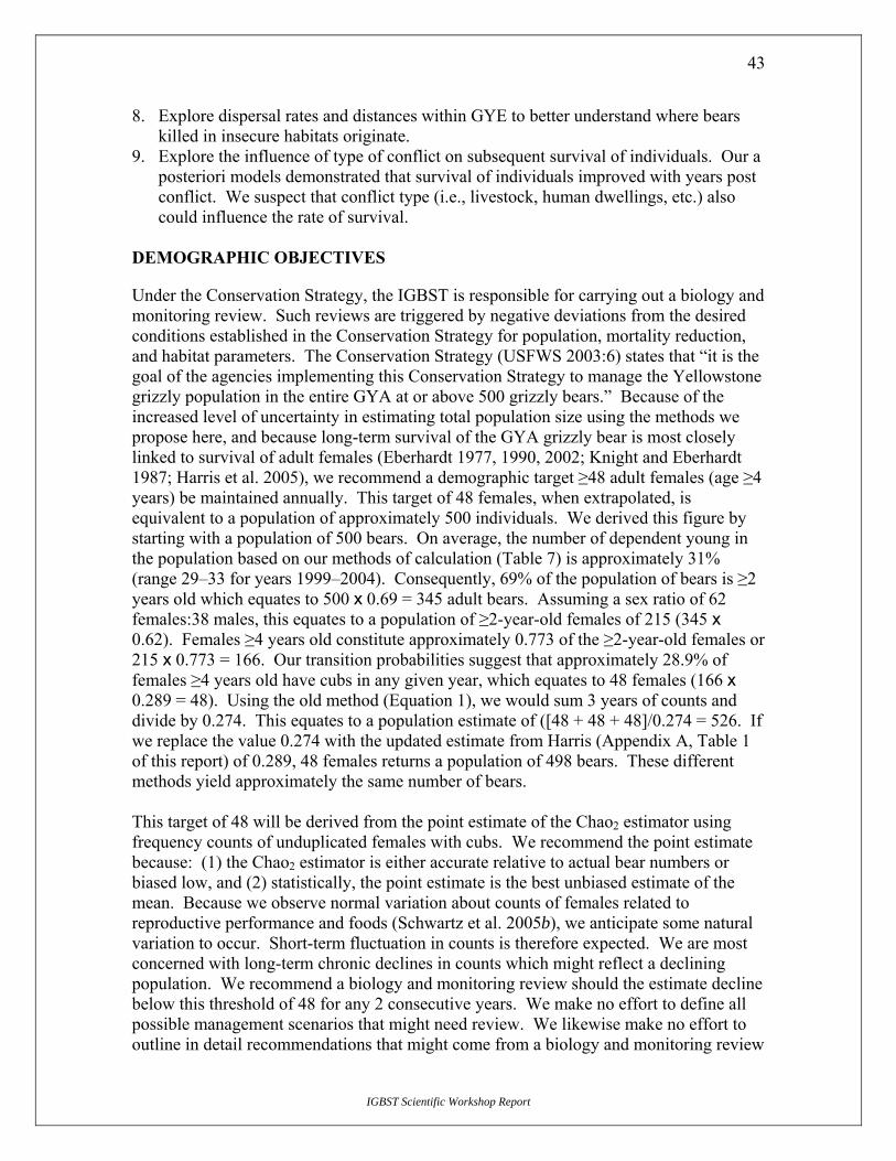
43

8. Explore dispersal rates and distances within GYE to better understand where bears killed in insecure habitats originate.

9. Explore the influence of type of conflict on subsequent survival of individuals. Our a posteriori models demonstrated that survival of individuals improved with years post conflict. We suspect that conflict type (i.e., livestock, human dwellings, etc.) also could influence the rate of survival.

DEMOGRAPHIC OBJECTIVES

Under the Conservation Strategy, the IGBST is responsible for carrying out a biology and monitoring review. Such reviews are triggered by negative deviations from the desired conditions established in the Conservation Strategy for population, mortality reduction, and habitat parameters. The Conservation Strategy (USFWS 2003:6) states that “it is the goal of the agencies implementing this Conservation Strategy to manage the Yellowstone grizzly population in the entire GYA at or above 500 grizzly bears.” Because of the increased level of uncertainty in estimating total population size using the methods we propose here, and because long-term survival of the GYA grizzly bear is most closely linked to survival of adult females (Eberhardt 1977, 1990, 2002; Knight and Eberhardt 1987; Harris et al. 2005), we recommend a demographic target ≥48 adult females (age ≥4 years) be maintained annually. This target of 48 females, when extrapolated, is equivalent to a population of approximately 500 individuals. We derived this figure by starting with a population of 500 bears. On average, the number of dependent young in the population based on our methods of calculation (Table 7) is approximately 31% (range 29–33 for years 1999–2004). Consequently, 69% of the population of bears is ≥2 years old which equates to 500 x 0.69 = 345 adult bears. Assuming a sex ratio of 62 females:38 males, this equates to a population of ≥2-year-old females of 215 (345 x 0.62). Females ≥4 years old constitute approximately 0.773 of the ≥2-year-old females or 215 x 0.773 = 166. Our transition probabilities suggest that approximately 28.9% of females ≥4 years old have cubs in any given year, which equates to 48 females (166 x 0.289 = 48). Using the old method (Equation 1), we would sum 3 years of counts and divide by 0.274. This equates to a population estimate of ([48 + 48 + 48]/0.274 = 526. If we replace the value 0.274 with the updated estimate from Harris (Appendix A, Table 1 of this report) of 0.289, 48 females returns a population of 498 bears. These different methods yield approximately the same number of bears.


This target of 48 will be derived from the point estimate of the Chao2 estimator using frequency counts of unduplicated females with cubs. We recommend the point estimate because: (1) the Chao2 estimator is either accurate relative to actual bear numbers or biased low, and (2) statistically, the point estimate is the best unbiased estimate of the mean. Because we observe normal variation about counts of females related to reproductive performance and foods (Schwartz et al. 2005b), we anticipate some natural variation to occur. Short-term fluctuation in counts is therefore expected. We are most concerned with long-term chronic declines in counts which might reflect a declining population. We recommend a biology and monitoring review should the estimate decline below this threshold of 48 for any 2 consecutive years. We make no effort to define all possible management scenarios that might need review. We likewise make no effort to outline in detail recommendations that might come from a biology and monitoring review

44

because each would have its own unique combination of circumstances and data that must be evaluated in light of other information. Management agencies lack complete control over female mortality. Hence, if the lower one-tailed 80% bound of the Chao2 estimate is <48 in any given year, agencies should attempt to limit female mortality the following year as a proactive measure to help minimize exceeding the point estimate recommendation above. Although male mortality has no impact on population trajectory over the long run (Harris et al. 2005), we feel that some limits are necessary. We therefore recommend that managers try not to exceed established mortality limits for males as set forth in this document. We recommend that a management review be considered should male limits be exceeded in any 3 consecutive years. We further recommend that mortality limits of dependent young not be exceeded in any 3 consecutive years.

ADAPTIVE MANAGEMENT

Dale Strickland provides a brief summary of adaptive management (West, Inc. 2005), which he gleaned from Holling (1978), McLain and Lee (1996), Walters (1997), and Holling and Allen (2002). Adaptive management (AM) is characterized as a 6-step feedback loop: 1. Assessment — the point where current understanding of the system leads to

development of strategies to meet management goals, prediction of outcomes of management, and the identification of key questions in the form of testable hypothesis.

2. Design — management actions and associated monitoring and research evaluate how well management meets specific management targets and address the hypothesis being tested.

3. Implementation — management is implemented according to the design. 4. Monitor — completed according to the design with data collected on specific

performance measures. 5. Evaluation — outcome is evaluated against predictions about effects of management;

progress toward goals is assessed. 6. Adjust — management adjusted based on evaluation of initial management actions.

This adjustment can range from slight modification of the management action to a complete change in management direction, and possibly a change in the overall focus of the management program.

An AM plan includes 3 critical elements: 1. Conceptual and quantitative models that make explicit the current understanding of

the system, the underlying hypotheses driving management, and key uncertainties; 2. Rigorous monitoring plans focused on reducing the most critical uncertainties and

clearly evaluating progress toward management goals; and


3. A scientifically defensible plan for monitoring and research and rapid feedback from management outcomes to revised management decisions.

45

AM usually sets limits on goals, objectives, and management flexibility. These limits are usually based on logistical and technological feasibility, costs, and laws and regulations. A major implication of adaptive management is that acquisition of useful data is one of the more important goals of management; therefore, the need for useful data should be considered when making management decisions. Monitoring and research should consider sources of uncertainty and attempt to reduce or eliminate them. However, the expected likelihood and costs of reducing uncertainty and the expected benefit in terms of improved management decisions will be primary considerations when prioritizing monitoring and research projects. This requires that setting of monitoring and research priorities is directly tied to the management framework. The Conservation Strategy (USFWS 2003) recommends using AM when possible. Our approach here follows those recommendations. Much of the original demographics work (Eberhardt et al. 1994, Eberhardt 1995, Boyce et al. 2001, Haroldson et al. 2005, Harris et al. 2005, Schwartz et al. 2005a, b, c) has been completed and meets the assessment set of the 6-step process. Development of strategies to meet management goals (in this case a sustainable population) is the objective of this document. We have formally developed testable hypotheses. Based upon recommendations here, our scientific hypothesis would be that recommended mortality limits based on methods to estimate population size and unknown and unreported mortality will result in a stable or slightly increasing population of grizzly bears in the GYE. Design elements for monitoring and continued research are contained within this document, as management recommendations to the demographics monograph (Schwartz et al. 2005c, and as part of the population monitoring recommendations of the Conservation Strategy (USFWS 2003). Annual reviews of results from all monitoring are recommended as per the Conservation Strategy.


The implementation phase is recommended to begin in 2005. Monitoring is ongoing and will continue. Counts of females with cubs and mortality documentation will be assessed annually for changes. Formal evaluation is recommended approximately every 8–10 years. Evaluation research will focus on updating demographic parameters used to estimate reproduction and survival, λ, and to reassess the stable age distribution, and transition probabilities used to estimate the number of females with cubs in any year. Should age structure, survival, or reproduction change due to density dependent relationships previously identified (Boyce et al. 2001, Schwartz et al. 2005a, b), or due to changes in food abundance or other natural processes adjustments to parameters used to estimate bear numbers, sustainable mortality, or unknown and unreported mortality will occur. Adjustments to this recommended protocol can occur after annual evaluations or following the more rigorous one that occurs every 8–10 years.

46

REPORT PREPARATION


We prepared this report to detail what we reviewed and our recommendations. We further recommend that results contained here be presented to state and federal managers for discussion, modification, and acceptance. Once this task is complete, we also recommend that these methods be presented to the Yellowstone Ecosystem Subcommittee for endorsement and application.

47

LITERATURE CITED

BLANCHARD, B. M., AND R. R. KNIGHT. 1991. Movements of Yellowstone grizzly bears, 1975–87. Biological Conservation 58:41–67.

BOYCE, M., B. M. BLANCHARD, R. R. KNIGHT, AND C. SERVHEEN. 2001. Population viability for grizzly bears: a critical review. International Association of Bear Research and Management Monograph Series Number 4.

BOULANGER, J., B. N. MCLELLAN, J. G. WOODS, M. E. PROCTOR, AND C. STROBECK. 2004. Sampling design and bias in DNA-based capture–mark–recapture population and density estimates of grizzly bears. Journal of Wildlife Management 68:457–46.

———, G. C. WHITE, B. N. MCLELLAN, J. WOODS, M. PROCTOR, AND S. HIMMER. 2002. A meta analysis of grizzly bear DNA mark–recapture projects in British Columbia. Ursus 13:137–152.

CHAO, A., W.-H. HWANG, Y.-C. CHEN, AND C.-Y. KUO. 2000. Establishing the number of shared species in two communities. Statistica Sinica 10:227–246.

———, M.-C. MA, AND M. C. K. YANG. 1993. Stopping rules and estimation for recapture debugging with unequal failure rates. Biometrika 80:193–201.

CHERRY, S., M. A. HAROLDSON, J. ROBISON-COX, AND C. C. SCHWARTZ. 2002. Estimating total human-caused mortality from reported mortality using data from radio-instrumented grizzly bears. Ursus 13:175–184.

EBERHARDT, L. L. 1977. Optimal policies for conservation of large mammals, with special reference to marine ecosystems. Environmental Conservation 4:205–212.

———. 1990. Survival rates required to sustain bear populations. Journal of Wildlife Management 54:587–590.

———. 1995. Population trend estimates from reproductive and survival data. Pages 13–19 in R. R. Knight and B. M. Blanchard, editors. Yellowstone grizzly bear investigations: annual report of the Interagency Study Team, 1994. National Biological Service, Bozeman, Montana, USA.

———. 2002. A paradigm for population analysis of long-lived vertebrates. Ecology 83:2841–2854.

———, B. M. BLANCHARD, AND R. R. KNIGHT. 1994. Population trend of the Yellowstone grizzly bear as estimated from reproductive and survival rates. Canadian Journal of Zoology 72:360–363.


———, AND R. R. KNIGHT. 1996. How many grizzlies in Yellowstone? Journal of Wildlife Management 60:416–421.

48

HAROLDSON, M. A., C. C. SCHWARTZ, AND G. C. WHITE. 2005. Survival of independent grizzly bear in the Greater Yellowstone Ecosystem, 1983–2001. In C. C. Schwartz, M. A. Haroldson, G. C. White, R. B. Harris, S. Cherry, K. A. Keating, D. Moody, and C. Servheen, authors. Temporal, spatial, and environmental influences on the demographics of grizzly bears in the Greater Yellowstone Ecosystem. Wildlife Monographs 161.

HARRIS, R. B. 1984. Harvest age structure as an indicator of grizzly bear population status. Thesis, University of Montana, Missoula, Montana, USA.

———. 1986. Modeling sustainable harvest rates for grizzly bears. Appendix K in A. Dood, R. Brannon, and R. Mace, editors. The grizzly bear in northwestern Montana. Final programmatic environmental impact statement. Montana Department of Fish, Wildlife and Parks, Helena, Montana, USA. Unit Publication, Missoula, Montana, USA.

———, C. C. SCHWARTZ, M. A. HAROLDSON, AND G. C. WHITE. 2005. Trajectory of the Yellowstone grizzly bear population under alternative survival rates. In C. C. Schwartz, M. A. Haroldson, G. C. White, R. B. Harris, S. Cherry, K. A. Keating, D. Moody, and C. Servheen, authors. Temporal, spatial, and environmental influences on the demographics of grizzly bears in the Greater Yellowstone Ecosystem. Wildlife Monographs 161.

HARRISON, J. L. 1958. Range of movement of some Malayan rats. Journal of Mammalogy 38:190–206.

HOLLING, C. S. 1978. Adaptive environmental assessment and management. John Wiley and Sons, New York, New York, USA.

———, AND C. R. ALLEN. 2002. Adaptive inference for distinguishing credible from incredible patterns in nature. Ecosystems 5:319–328.

KEATING, K. A., C. C. SCHWARTZ, M. A. HAROLDSON, AND D. MOODY. 2002. Estimating numbers of females with cubs-of-the-year in the Yellowstone grizzly bear population. Ursus 13:161–174.

KNIGHT, R. R., B. M. BLANCHARD, AND L. L. EBERHARDT. 1995. Appraising status of the Yellowstone grizzly bear population by counting females with cubs-of-the-year. Wildlife Society Bulletin 23:245–248.

———, AND L. L. EBERHARDT. 1985. Population dynamics of Yellowstone grizzly bears. Ecology 66:323–334.


———, AND ———. 1987. Prospects for Yellowstone grizzly bears. International Conference on Bear Research and Management 7:45–50.

49

MATTSON, D. M. 1997. Sustainable grizzly bear mortality calculations from counts of females with cubs-of-the-year: an evaluation. Biological Conservation 81:103–111.

———, R. R. KNIGHT, AND B. M. BLANCHARD. 1987. The effects of developments and primary roads on grizzly bear habitat use in Yellowstone National Park, Wyoming. International Conference on Bear Research and Management 7:259–273.

MCKELVEY, K. S., AND M. K. SCHWARTZ. 2004. Genetic errors associated with population estimation using non-invasive molecular tagging: problems and new solutions. Journal of Wildlife Management 68:439–448.

MCLAIN, R. J. AND R. G. LEE. 1996. Adaptive management: promises and pitfalls. Environmental Management 20:437–448.

MCLOUGHLIN, P. D. 2002. Managing risks of decline for hunted populations of grizzly bears given uncertainty in population parameters. Final Report. British Columbia Independent Scientific Panel on Grizzly Bears. Report to the British Columbia Independent Research Panel on Grizzly Bears, Victoria, British Columbia, Canada.

MILLER, S. D., G. C. WHITE, R. A. SELLERS, H. V. REYNOLDS, J. W. SCHOEN, K. TITUS, V. BARNES, JR., R. B. SMITH, R. R. NELSON, W. B. BALLARD, AND C. C. SCHWARTZ. 1997. Brown and black bear density estimation in Alaska using radiotelemetry and replicated mark–resighting techniques. Wildlife Monographs 133.

MILLS, L. S., J. J. CITTA, K. P. LAIR, M. K. SCHWARTZ, AND D. A. TALLMON. 2000. Estimating animal abundance using non-invasive DNA sampling: promise and pitfalls. Ecological Applications 10:283–294.

MOWAT, G., AND C. STROBECK. 2000. Estimating population size of grizzly bears using hair capture, DNA profiling, and mark–recapture analysis. Journal of Wildlife Management 64:183–193.

PAETKAU, D. 2003. An empirical exploration of data quality in DNA-based population inventories. Molecular Ecology 12:1375–1387.

———. 2004. The optimal number of makers in genetic capture–mark–recapture studies. Journal of Wildlife Management 68:449–452.


SCHWARTZ, C. C. 1999. Evaluation of a capture–mark–recapture estimator to determine grizzly bear numbers and density in the Greater Yellowstone Area. Pages 13–20 in C. C. Schwartz and M. A. Haroldson, editors. Yellowstone grizzly bear investigations: annual report of the Interagency Grizzly Bear Study Team, 1998. U.S. Geological Survey, Bozeman, Montana, USA.

50

———. 2000. Evaluation of a capture–mark–recapture estimator to determine grizzly bear numbers and density in the Greater Yellowstone Area. Pages 15–18 in C. C. Schwartz and M. A. Haroldson, editors. Yellowstone grizzly bear investigations: annual report of the Interagency Grizzly Bear Study Team, 1999. U.S. Geological Survey, Bozeman, Montana, USA.

———, AND A. W. FRANZMANN. 1991. Interrelationship of black bears to moose and forest succession in the northern coniferous forest. Wildlife Monographs 113.

———, M. A. HAROLDSON, AND S. CHERRY. 2005a. Reproductive performance for grizzly bears in the Greater Yellowstone Ecosystem, 1983–2002. In C. C. Schwartz, M. A. Haroldson, G. C. White, R. B. Harris, S. Cherry, K. A. Keating, D. Moody, and C. Servheen, authors. Temporal, spatial, and environmental influences on the demographics of grizzly bears in the Greater Yellowstone Ecosystem. Wildlife Monographs 161.

———, ———, K. A. GUNTHER, AND D. MOODY. 2002. Distribution of grizzly bears in the Greater Yellowstone Ecosystem, 1990–2000. Ursus 13:203–212.

———, ———, AND G. C. WHITE. 2005e. Study area and methods for collecting and analyzing demographic data on grizzly bears in the Greater Yellowstone Ecosystem. In C. C. Schwartz, M. A. Haroldson, G. C. White, R. B. Harris, S. Cherry, K. A. Keating, D. Moody, and C. Servheen, authors. Temporal, spatial, and environmental influences on the demographics of grizzly bears in the Greater Yellowstone Ecosystem. Wildlife Monographs 161.

———, ———, AND ———. 2005b. Survival of cub and yearling grizzly bears in the Greater Yellowstone Ecosystem, 1983–2001. In C. C. Schwartz, M. A. Haroldson, G. C. White, R. B. Harris, S. Cherry, K. A. Keating, D. Moody, and C. Servheen, authors. Temporal, spatial, and environmental influences on the demographics of grizzly bears in the Greater Yellowstone Ecosystem. Wildlife Monographs 161.

———, ———, ———, R. B. HARRIS, S. CHERRY, K. A. KEATING, D. MOODY, AND C. SERVHEEN. 2005d. Temporal, spatial, and environmental influences on the demographics of grizzly bears in the Greater Yellowstone Ecosystem. In C. C. Schwartz, M. A. Haroldson, G. C. White, R. B. Harris, S. Cherry, K. A. Keating, D. Moody, and C. Servheen, authors. Wildlife Monographs 161.


———, R. B. HARRIS, AND M. A. HAROLDSON. 2005c. Impacts of spatial and environmental heterogeneity on grizzly bear demographics in the Greater Yellowstone Ecosystem: a source–sink dynamic with management consequences. In C. C. Schwartz, M. A. Haroldson, G. C. White, R. B. Harris, S. Cherry, K. A. Keating, D. Moody, and C. Servheen, authors. Temporal, spatial, and environmental influences on the demographics of grizzly bears in the Greater Yellowstone Ecosystem. Wildlife Monographs 161.

51

U.S. FISH AND WILDLIFE SERVICE. 1982. Grizzly bear recovery plan. U.S. Fish and Wildlife Service, Denver, Colorado, USA.

———. 1993. Grizzly bear recovery plan. U.S. Fish and Wildlife Service, Missoula, Montana, USA.

———. 2003. Final conservation strategy for the grizzly bear in the Greater Yellowstone Ecosystem. U.S. Fish and Wildlife Service, Missoula, Montana, USA.

VAN BELLE, G. 2002. Statistical rules of thumb. John Wiley and Sons, New York, New York, USA.

WAITS, L. P. 2004. Using non-invasive genetic sampling to detect and estimate abundance of rare wildlife species. Pages 211–228 in W. L. Thompson, editor. Sampling rare or elusive species. Island Press, Washington, D.C., USA.

———, AND D. PAETKAU. 2005. Non-invasive genetic sampling tools for wildlife biologists: a review of applications and recommendations for accurate data collection. Wildlife Society Bulletin 33:in press.

WALTERS, C. 1997. Challenges in adaptive management of riparian and coastal ecosystems. Conservation Ecology 1(2):1. http://www.consecol.org/vol1/iss2/art1

WEST, INC. 2005. Avian collision and electrocution risk reduction adaptive management plan for the Altamont Pass Wind Resource Area. Technical Report. West Incorporated, Laramie, Wyoming, USA.

WHITE, G. C. 1996. NOREMARK: population estimation from mark–resighting surveys. Wildlife Society Bulletin 24:50–52.

———, D. R. ANDERSON, K. P. BURNHAM, AND D. L. OTIS. 1982. Capture–recapture and removal methods for sampling closed populations. Los Alamos National Laboratory report LA-8787-NEPA. Los Alamos National Laboratory, Los Alamos, New Mexico, USA.


WOODS, J. G., D. PAETKAU, D. LEWIS, B. N. MCLELLAN, M. PROCTOR, AND C. STROBECK. 1999. Genetic tagging of free-ranging black and brown bears. Wildlife Society Bulletin 27:616–627.

http://www.consecol.org/vol1/iss2/art1

52

Appendix A

Age-structures of modeled Greater Yellowstone Ecosystem grizzly bear populations

Appendix to Final Report

16 April 2003

Richard B. Harris, Ph.D

218 Evans Missoula, Montana USA 59801

(406) 542-6399 [email protected]

in partial fulfillment of

U.S. Geological Survey agreement with USFWS 01-R6-01 Order No. 02CRSa0331

Reference No. 02CRPR00569 The bulk of work completing this contract is contained in the report “Trajectory of the Yellowstone grizzly bear population under alternative survival rates,” which is also being submitted for publication. This Appendix deals, separately, with the work pursuant to the last named deliverable: “Estimates and confidence limits around the proportion of the Greater Yellowstone Ecosystem (GYE) grizzly bear population consisting of adult females will also be produced as part of this work. Such estimates and confidence limits are a necessary component of estimates of total grizzly bear population size.” Objective Size of the GYE grizzly bear population is currently estimated by dividing the estimate of “adult females” by the constant 0.284 (USFWS 1993:42). It is desirable to evaluate whether this constant is appropriate, and whether it should be updated. As well, use of a constant ignores the fact that this proportion may vary among years, and thus total population size should be estimated with appropriate error terms. Here, I employed simulation techniques used in Harris et al. (2005) to update estimates that may be useful should managers desire to estimate total population size from some index of females with cubs or females of a minimum age. Methods


Analyses of population parameters and development of a simulation model are both described in Harris et al. (2005), Schwartz et al. (2005a, b), and Haroldson et al. (2005). To generate statistics for this report, I used 2 parameterizations of the full simulation: (1) mean adult female (age >2) survival at 0.949, adult male (age >2) survival at 0.874, and

mailto:[email protected]

53

yearly process variation of survival rates approximating the shrunk estimates of process variation for the data set in which bears with unresolved fates were censored at last contact (Haroldson et al. 2005:Table 13); and (2) mean adult female (age >2) survival at 0.922, adult male (age >2) survival at 0.823, and yearly process variation of survival rates approximating the shrunk estimates of process variation from the data set in which animals with unresolved fates were assumed to have died (Haroldson et al. 2005). For each parameter set, I used a model run of 10 years (paralleling the larger analysis) and performed 3,000 iterations. The resulting proportions come from a sample of 30,000 years (there is some dependence of proportions within each 10-year series). Results are summarized via 5 statistics, determined yearly: (1) proportion of females in the population with cubs-of-the-year (cubs, hereafter); (2) proportion of all females aged >2 with cubs; (3) proportion of females aged >4 with cubs; (4) proportion of females aged >5 with cubs; and (5) proportion of the total population consisting of females aged >5. Results Proportions of females with cubs in any given year, and by females in the presumptive “adult” ages of 5 and older are shown in Tables 1 and 2 for the 2 alternative parameter sets. Values were very similar for both simulations. The mean proportion of the total population consisting of adult females varied from 0.29 to 0.30, which are both similar to the earlier assumed value of 0.284. Without simulations, values of the proportion of the female segment made up by females with cubs in any year were not previously available. Table 1. Proportions generated from age-structures of simulated populations with high survival and low process variance.

Mean CVaLower

95% CL Upper

95% CL

Proportion of all females that are with cubs 0.176 0.097 0.145 0.212

Proportion of female 2+ that are with cubs 0.247 0.110 0.199 0.307



Proportion of total population that are females age ≥5 0.289 0.047 0.266 0.319 a Standard deviation/mean.

Table 2. Proportions generated from age-structures of simulated populations with low survival and high process variance.

Mean CVa

Lower 95% CL

Upper95% CL

Proportion of all females that are with cubs 0.176 0.094 0.143 0.209




Proportion of total population that are females age ≥5 0.299 0.036 0.278 0.320


a Standard deviation/mean.

54

Discussion Variability of the figures provided in Tables 1 and 2 may be slightly lower than reality, because cub production varied independently each year, and variance was modeled as coming from a single distribution that was normal on the logit scale. In reality, we suspect that some very poor food years are characterized by near complete failure to breed of all available females (i.e., those of sufficient maturity who do not have cubs or yearlings from previous years at their sides). The year following such a failure, there is probably a bumper crop of cubs, because those females failing to breed during the poor year are added to those who would have been available in any case. Thus, there is probably more variability in the true ratio of females with cubs to all females than represented in these simulations. Even were that variation to be included, coefficients of variation and confidence limits (Table 1, 2) depict variation of the entire population (i.e., reflect process variation). They do not reflect the variability that will characterize samples of the population, the magnitude of which will depend on sample size. It would seem more straight forward to estimate the number of females from females with cubs, than the current alternative (estimating total population size from adult females). This is because the yearly estimates of the number of females with cubs do not correspond exactly to females of any particular age. Age at first reproduction is not a step function, but rather a gradually increasing function (Schwartz et al. 2005a). As well, breeding interval, although close to 3 years, is itself variable. Thus, additional assumptions and approximation are necessary to convert females with cubs into “adult” females. In contrast, the ratio of females with cubs:all females does not require additional assumptions or approximations (beyond those included in the simulation model). In addition, estimating the size and trend of the female segment of the population is probably more informative for conservation and management purposes than is estimating total population size. Acknowledgments Thanks to C. Schwartz, M. Haroldson, G. White, S. Cherry, and K. Keating for helpful discussion. Literature Cited HAROLDSON, M. A., C. C. SCHWARTZ, AND G. C. WHITE. 2005. Survival of independent

grizzly bear in the Greater Yellowstone Ecosystem, 1983–2001. In C. C. Schwartz, M. A. Haroldson, G. C. White, R. B. Harris, S. Cherry, K. A. Keating, D. Moody, and C. Servheen, authors. Temporal, spatial, and environmental influences on the demographics of grizzly bears in the Greater Yellowstone Ecosystem. Wildlife Monographs 161.


HARRIS, R. B., C. C. SCHWARTZ, M. A. HAROLDSON, AND G. C. WHITE. 2005. Trajectory of the Yellowstone grizzly bear population under alternative survival rates. In C. C. Schwartz, M. A. Haroldson, G. C. White, R. B. Harris, S. Cherry, K. A. Keating, D. Moody, and C. Servheen, authors. Temporal, spatial, and

55

environmental influences on the demographics of grizzly bears in the Greater Yellowstone Ecosystem. Wildlife Monographs 161.

SCHWARTZ, C. C., M. A. HAROLDSON, AND S. CHERRY. 2005a. Reproductive performance for grizzly bears in the Greater Yellowstone Ecosystem, 1983–2002. In C. C. Schwartz, M. A. Haroldson, G. C. White, R. B. Harris, S. Cherry, K. A. Keating, D. Moody, and C. Servheen, authors. Temporal, spatial, and environmental influences on the demographics of grizzly bears in the Greater Yellowstone Ecosystem. Wildlife Monographs 161.

———, ———, AND G. C. WHITE. 2005b. Survival of cub and yearling grizzly bears in the Greater Yellowstone Ecosystem, 1983–2001. In C. C. Schwartz, M. A. Haroldson, G. C. White, R. B. Harris, S. Cherry, K. A. Keating, D. Moody, and C. Servheen, authors. Temporal, spatial, and environmental influences on the demographics of grizzly bears in the Greater Yellowstone Ecosystem. Wildlife Monographs 161.


U.S. FISH AND WILDLIFE SERVICE. 1993. Grizzly bear recovery plan. Missoula, Montana, USA.

56

Appendix B Counts and estimates of mortality for independent-aged grizzly bears in the Greater

Yellowstone Ecosystem

Mark Haroldson Interagency Grizzly Bear Study Team

U.S. Geological Survey, Northern Rocky Mountain Science Center Bozeman, Montana

and

Steve Cherry

Department of Mathematical Sciences Montana State University

Bozeman, Montana Grizzly bears (Ursus arctos horribilis) in the Greater Yellowstone Ecosystem (GYE) are currently listed as threatened under the Endangered Species Act. Tracking mortality in the population is an essential component of the recovery process. Grizzly bear deaths caused by agency removals or those of instrumented bears are known or can be inferred. Additionally, the public reports an unknown portion of mortalities of uncollared bears. Cherry et al. (2002) described methodology to estimate the number of nonagency human-caused deaths of uncollared bears using a hierarchical Bayesian model with a noninformative prior distribution for the number of deaths. Critical assumptions relative to the method were identified in Cherry et al. (2002). We applied methodology developed in Cherry et al. (2002) to estimate annual unreported mortality, from all causes, for independent aged female and male bears. We excluded possible mortalities (Craighead et al. 1988) from consideration because by definition the chance is small that these instances resulted in dead bears. Also, since we estimated for all mortalities regardless of cause, known deaths from undetermined causes are included. Cherry et al. (2002) alternately included or excluded unexplained and unresolved losses of radiomarked bears to estimate reporting rates. We used a Delphi procedure to identify which unexplained and unresolved losses were likely mortalities. Nine experts who manage or research grizzly bears in the GYE ranked each unexplained and unresolved loss as whether it was, in their opinion, a human-caused mortality. Results of this Delphi procedure suggested that 41% (9/22) of these unexplained and unresolved losses were likely human-caused mortalities and are included as such in subsequent analyses.


We combined sexes to estimate reporting rate because there was no evidence that rates were different between sexes (Table 1). We used estimates of reporting rates developed from deaths of radiomarked bears from 1983–2004 to develop prior probability distributions that the public reported bear mortalities regardless of cause.

57

Table 1. Method of discovery for deaths of independent (ages ≥2 years) radiomarked grizzly bears during 1983-2004, regardless of cause. Estimated reporting rate is 37%, conversely 63% of mortalities of radiomarked bears go unreported.

Method of discovery Frequency %

Unreported (discovery due to telemetry) 36 63.2

Reported (discovery not due to telemetry) 21 36.8

Total 57 100

The number of publicly reported deaths of uncollared bears, together with the beta distribution estimated from the observed reporting rate, are used to estimate a posterior distribution for total annual reported and unreported mortality (Cherry et al. 2002). We used the median of the posterior distribution (Appendix D) as our best estimate of unreported mortality (Table 2, 3). Number of management removals and losses of radiomarked bears documented annually are added to the median estimate of reported and unreported mortality to estimate total annual mortality from all causes.


58

Table 2. Mortality counts and estimates for independent female deaths, 1986–2004.

Year

Sanctioneda

removals

Radiomarkedb

loss

Reportedc

loss

Reported andd

unreported loss (median)

Totale

mortality 1986 1 3 1 2 6 1987 1 0 1 2 3 1988 0 1 0 1 2 1989 0 0 0 1 1 1990 1 2 3 7 10 1991 0 0 0 1 1 1992 0 1 0 1 2 1993 0 1 2 5 6 1994 0 2 1 2 4 1995 3 0 3 7 10 1996 1 3 2 5 9 1997 0 0 3 7 7 1998 0 0 1 2 2 1999 0 0 1 2 2 2000 1 1 3 7 9 2001 5 3 1 2 10 2002 2 2 4 10 14 2003 1 0 5 13 14 2004 4 0 5 13 17

a Includes removals of radiomarked bears. b Losses of radiomarked bears from all causes except sanctioned management removals. c Reported losses from all causes excluding sanctioned management removals and radiomarked

bears. d Median of creditable interval for reported and unreported loss estimates using methodology

described in Cherry et al. (2002). e Total mortality is the sum of sanctioned removal plus radiomarked loss plus the median for

reported and unreported loss.


59

Table 3. Mortality counts and estimates for independent male deaths, 1986–2004.

Year

Sanctioneda

removals

Radiomarkedb

loss

Reportedc

loss

Reported andd

unreported loss (median)

Totale

mortality 1986 1 1 0 1 3 1987 2 1 0 1 4 1988 1 1 1 2 4 1989 1 1 1 2 4 1990 1 1 2 5 7 1991 0 0 0 1 1 1992 2 5 1 2 9 1993 0 2 0 1 3 1994 0 1 1 2 3 1995 2 4 4 10 16 1996 2 2 3 7 11 1997 1 1 2 5 7 1998 2 2 0 1 5 1999 2 2 3 7 11 2000 2 4 11 29 35 2001 7 2 1 2 11 2002 4 1 3 7 12 2003 2 3 3 7 12 2004 3 2 7 18 23

a Includes removals of radiomarked bears. b Losses of radiomarked bears from all causes except sanctioned management removals. c Reported losses from all causes excluding sanctioned management removals and radiomarked

bears. d Median of creditable interval for reported and unreported loss estimates using methodology

described in Cherry et al. (2002). e Total mortality is the sum of sanctioned removal plus radiomarked loss plus the median for

reported and unreported loss. Literature Cited CHERRY, S., M. A. HAROLDSON, J. ROBISON-COX, AND C. C. SCHWARTZ. 2002.

Estimating total human-caused mortality from reported mortality using data from radio-instrumented grizzly bears. Ursus 13:175–184.


CRAIGHEAD, J. J., K. R. GREER, R. R. KNIGHT, AND H. I. PAC. 1988. Grizzly bear mortalities in the Yellowstone Ecosystem, 1959–1987. Montana Department of Fish, Wildlife and Parks, Helena, Montana, USA, Craighead Wildlife Institute, Missoula, Montana, USA, Interagency Grizzly Bear Study Team, Bozeman, Montana, USA, and National Fish and Wildlife Foundation, Washington, D. C., USA.

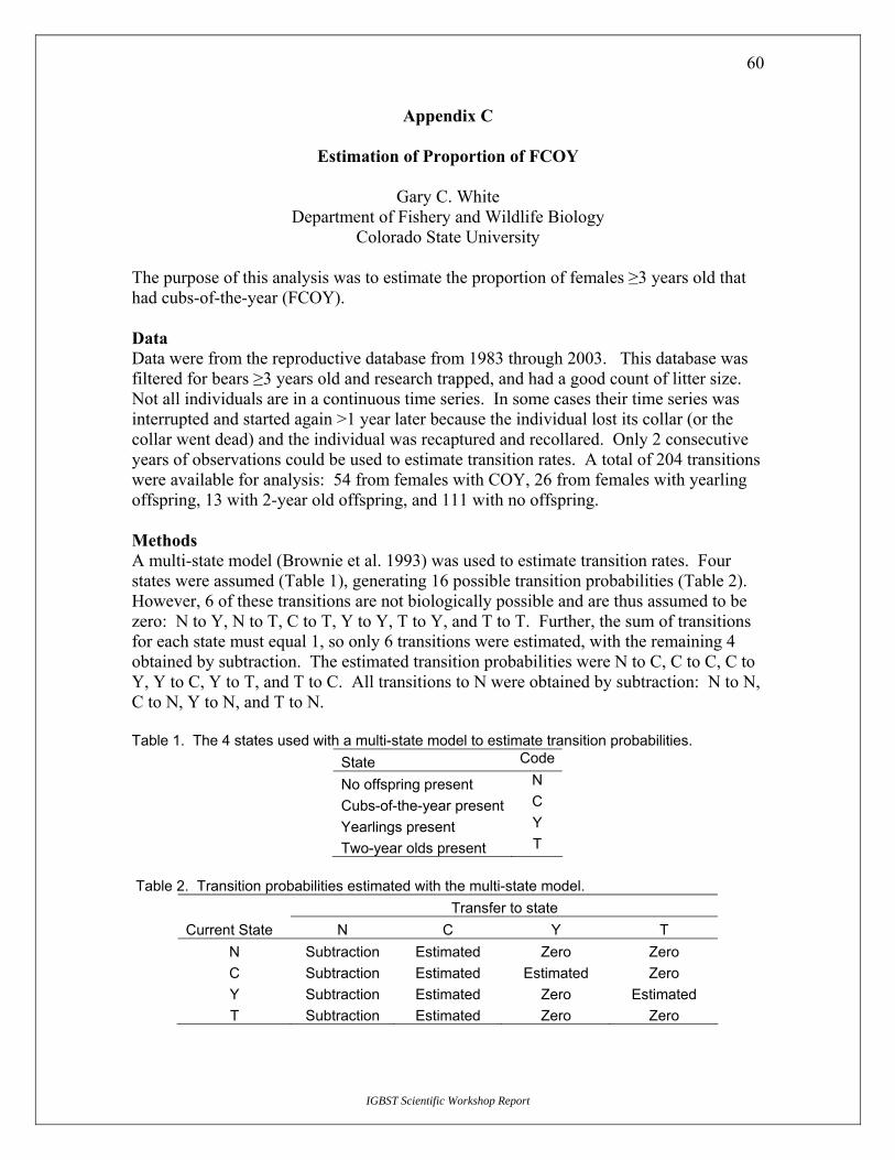
60

Appendix C

Estimation of Proportion of FCOY

Gary C. White Department of Fishery and Wildlife Biology

Colorado State University

The purpose of this analysis was to estimate the proportion of females ≥3 years old that had cubs-of-the-year (FCOY). Data Data were from the reproductive database from 1983 through 2003. This database was filtered for bears ≥3 years old and research trapped, and had a good count of litter size. Not all individuals are in a continuous time series. In some cases their time series was interrupted and started again >1 year later because the individual lost its collar (or the collar went dead) and the individual was recaptured and recollared. Only 2 consecutive years of observations could be used to estimate transition rates. A total of 204 transitions were available for analysis: 54 from females with COY, 26 from females with yearling offspring, 13 with 2-year old offspring, and 111 with no offspring. Methods A multi-state model (Brownie et al. 1993) was used to estimate transition rates. Four states were assumed (Table 1), generating 16 possible transition probabilities (Table 2). However, 6 of these transitions are not biologically possible and are thus assumed to be zero: N to Y, N to T, C to T, Y to Y, T to Y, and T to T. Further, the sum of transitions for each state must equal 1, so only 6 transitions were estimated, with the remaining 4 obtained by subtraction. The estimated transition probabilities were N to C, C to C, C to Y, Y to C, Y to T, and T to C. All transitions to N were obtained by subtraction: N to N, C to N, Y to N, and T to N. Table 1. The 4 states used with a multi-state model to estimate transition probabilities.

State Code

No offspring present N

Cubs-of-the-year present C

Yearlings present Y

Two-year olds present T

Table 2. Transition probabilities estimated with the multi-state model.

Transfer to state Current State N C Y T

N Subtraction Estimated Zero Zero C Subtraction Estimated Estimated Zero Y Subtraction Estimated Zero Estimated T Subtraction Estimated Zero Zero


61

Estimation was performed with Program MARK (White and Burnham 1999) using the Brownie et al. (1993) multi-state model with maximum likelihood estimation and information-theoretic procedures for model selection (Burnham and Anderson 2002). Because only consecutive observations were analyzed, survival and capture probability parameters in the model were set to 1 and not estimated. Animals were removed from analysis after their last observation. A time-varying covariate of age of the female was included in 2 multi-state models to evaluate the effect of age on transition probabilities using a logit link. A model with each transition modeled with its own intercept and linear age effect on a logit scale was considered, followed by a model with each transition modeled with its own intercept, age and age-squared effects on a logit scale. Based on results from these models, additional post hoc, reduced models were considered where the results from the age and age-squared models suggested terms to remove that did not contribute to the fit of the model to the data. Time-specific models of the transition probabilities were not considered because of limited data available across the 21 years of observations. For the model with transition probabilities constant across time and no age covariate, the transition probabilities can be estimated directly from multinomial distributions, with this approach used to verify the estimates from Program MARK. To estimate the proportion of the population in each state if the transition probabilities are assumed to be constant across time, the matrix of transition probabilities was raised to the 50th power and multiplied by the vector [1, 0, 0, 0]. The variance–covariance of the resulting vector was obtained numerically with the delta method. Results The models estimated and the model selection results (Table 3) suggest that age was an important predictor of transition probabilities. Estimates of the 6 transition probabilities for the intercept only model (no age effects) are provided in Table 4.


Table 3. Results of model selection conducted in Program MARK for the 3 models considered a priori (bottom 3 models) and the 3 additional models (top 3 models) considered post priori to estimate 6 transition probabilities.

Model AICc Delta AICc

AICc weights

Model likelihood

Num. par Deviance

{psi(Age(Y to C, Y to T) *Transition*Age^2(N to C ))} 303.384 0 0.63188 1 10 282.341 {psi(Age*Transition*Age^2 for N to C, Y to C, and Y to T)} 305.605 2.2207 0.20817 0.3294 12 280.112 {psi(Age*Transition +N to C Age^2)} 306.213 2.8293 0.15355 0.243 13 278.463 {psi(Age*Transition*Age^2)} 314.222 10.8376 0.0028 0.0044 18 274.852 {psi(Constant)} 314.487 11.1034 0.00245 0.0039 6 302.097 {psi(Age*Transition)} 315.998 12.6137 0.00115 0.0018 12 290.505

62

Table 4. Estimates of the 6 transition probabilities from the likelihood analysis of the constant model in Table 3. Transition probability Estimate SE LCI UCI N to C 0.475 0.045586 0.387371 0.564196 C to C 0.033898 0.02356 0.008493 0.125662 C to Y 0.79661 0.052404 0.675093 0.88071 Y to C 0.103448 0.056552 0.033745 0.276003 Y to T 0.689655 0.085909 0.502948 0.829943 T to C 0.642857 0.12806 0.376261 0.84304

The matrix of transition probabilities, including estimates obtained by subtraction, are shown in Table 5. In Table 6 are the estimates of the proportion of the population that would exist in each state assuming that transition probabilities are constant across time and age.

Table 5. Matrix of transition probability estimates. Transfer to state Current state N C Y T N 0.525 0.475 0 0 C 0.169492 0.033898 0.79661 Y 0.206897 0.103448 0 0.689655 T 0.357143 0.642857 0 0

Table 6. Asymptotic proportion of females in each state, with associated SE and 95% confidence intervals. State Estimate SE LCI UCI N 0.322529 0.056233 0.212313 0.432745 C 0.288777 0.022984 0.243728 0.333827 Y 0.230043 0.02362 0.183748 0.276338 T 0.158650 0.025705 0.108269 0.209032

Discussion From Table 6, I conclude that 28.9% of the female population ≥4 years of age (recall I measured transitions, so bears starting at age 3 transitioned to age 4) will have cubs-of-the-year. This estimate is not affected by bias in the initial captures of the radiomarked sample. Suppose that the state of newly radiocollared animals is not in proportion to what exists in the population because some states are more likely to be trapped than others. For example, suppose that females in the N state are most likely to be collared, whereas females with offspring present are less likely. The sample used in the analysis will be weighted heavily toward the trappable state. However, estimates of the transitions are conditional on the current state. So although sample sizes will not be proportional to the actual frequencies of the states in the population, the estimates are not biased by this discrepancy in the frequency of states in the sample compared to the population. The precision of the estimates in Table 4 reflects the sample sizes available to estimate each transition.


63

If the frequency of the class transitioned from in the 204 transitions used in the analysis had been used to estimate the proportion of the population in each state, the estimates would have been N 0.544, C 0.265, Y 0.128, and T 0.064. These estimates differ substantially from the values in Table 6, and bias in capture frequencies. For the 74 captures of females where a radiocollar was attached, the proportions were N 0.663, C 0.229, Y 0.084, and T 0.024. These estimates of the proportion of each class captured to be radiocollared suggest that the most likely state to be captured in the sample is N, where the female is not encumbered by offspring. However, a potential source of bias exists if radiocollared animals slip or otherwise lose their collars (possibly from death) at different rates. In particular, if females about to make a particular transition, say Y to T, are more likely to lose their radiocollars than females in other states, biased estimates of the transition probabilities will result because of this disproportional censoring, and hence biased estimates of the proportion of females in each state will result. Of the 80 losses (i.e., loss of collar or death of the female), 0.263 occurred for N, 0.400 for C, 0.250 for Y, and 0.088 for T. These values are intermediate between the estimated asymptotic distribution (Table 6) and the frequency of females collared (Fig. 1). The proportion of collars lost seems to be the highest for females with offspring, particularly cubs-of-the-year. Possibly the loss of collars for FCOY is higher because of weight loss from the energetic costs of suckling cubs.

0

0.1

0.2

0.3

0.4

0.5

0.6

0.7

N C Y T

State

Prop

ortio

n `

AsymptoticFrom StateCollar LossCaptures

Figure 1. Proportion of females in each state for 4 estimates: “asymptotic values” are proportion of females estimated from the multi-state analysis, “from state” is the proportion of the 4 states from which the transitions were estimated, “collar loss” is the proporiton of each state losing collars, and “captures” is the proportion of each state in the sample when the animals were captured and radiocollared.


Age was important in model selection results (Table 3), particularly for the N to C transition when modeled as a quadratic. Graphs of the transition functions (Fig. 2) suggest evidence that older animals became better mothers, more capable of raising cubs to independent offspring. The transition rates of both C to Y and Y to T are increasing

64

early with age, and then declining at older ages. If older, more mature females become better mothers, I expect that both these transitions should increase with experience. Both C to C and Y to C transitions decrease with age, which is expected under the hypothesis of older females being better mothers. The graph for N to C (Fig. 2) also suggests that the most fertile females are of medium age, as suggested by the C to Y and Y to T curves.

{psi Age*Transition*Age^2}

0

0.1

0.2

0.3

0.4

0.5

0.6

0.7

0.8

0.9

1

0 5 10 15 20 25

Age

Tran

sitio

n ` psi N to C

psi C to Cpsi C to Ypsi Y to Cpsi Y to Tpsi T to C

Figure 2. Age-specific transition probabilities from the quadratic model {psi(Age*Transition*Age^2)}. Because the {psi(age x transition x age2)} model has 18 parameters, a more parsimonious model was sought to use in modeling age effects in a population model. The top AICc model obtained post posteriori was {psi(age(Y to C, Y to T) x transition x age2(N to C ))}, where the Y to C and Y to T transitions were modeled as a linear function of age, N to C was a quadratic function of age, and the remaining transition probabilities were assumed constant (Fig. 3). This is the model that will be used to develop an age-structured model for evaluating the consistency of various estimates of survival, population size, and recruitment.


65

{psi(Age(Y to C, Y to T)*Transition*Age^2(N to C ))}

0

0.1

0.2

0.3

0.4

0.5

0.6

0.7

0.8

0.9

0 5 10 15 20 25

Age

Tran

sitio

n `

psi N to Cpsi C to Cpsi C to Ypsi Y to Cpsi Y to Tpsi T to C

Figure 3. Transition probabilities as a function of age from the model {psi(age(Y to C, Y to T) x transition x age2(N to C ))}. Literature Cited BROWNIE, C., J. E. HINES, J. D. NICHOLS, K. H. POLLOCK, AND J. B. HESTBECK. 1993.

Capture–recapture studies for multiple strata including non-Markovian transitions. Biometrics 49:1173–1187.

BURNHAM, K. P., AND D. R. ANDERSON. 2002. Model selection and multimodel

inference: a practical information-theoretic approach. Springer-Verlag, New York, New York, USA.


WHITE, G. C., AND K. P. BURNHAM. 1999. Program MARK: survival estimation from populations of marked animals. Bird Study 46 Supplement:120–138.

66

Appendix D Point Estimation using the Total Mortality Estimator

Steve Cherry

Department of Mathematical Sciences Montana State University

Bozeman, Montana

The proposed method of estimating total mortality given a number of known and probable reported mortalities leads to a posterior distribution of total mortality. There are a number of ways of summarizing the information in this distribution to arrive at a point estimate of total mortality. Three common summaries are the mean, median, and mode of the distribution. These estimators are derived assuming different costs of being wrong. The cost of being wrong is quantified in a loss function, and an estimator is derived for each loss function by finding the one which minimizes average loss. Each estimator is briefly discussed below. Mean The loss function is referred to as squared error loss and the goal is to find an estimator

which minimizes where the E refers to a probabilistic averaging operation. The best estimator is the mean of the posterior distribution, N̂ ( 2

N̂NE − )

( )∑∞

=

==0

ˆn

nNnPN .

Median The loss function is referred to as absolute error loss and the goal is to find an estimator

which minimizes N̂ NNE ˆ− . The best estimator is the median of the posterior

distribution. We actually chose to be the value of the posterior distribution that is smallest value of n such that

N̂P N ≤ n( )≥ 0.5.

Mode The loss function (L) is a 0/1 loss function, where 1=L if and if . The mean of this loss function is the mode of the posterior distribution. The mode is the value of N that has the highest probability associated with it.

NN ˆ= 0=L NN ˆ≠


There are other possible loss functions, but these 3 are the most commonly used. If the number of reported losses is small, the posterior is skewed to the right and the median is a better summary measure of center than the mean. As the number of reported losses increases, the posterior distribution becomes more symmetric and the median and mean give essentially the same result. Using the mode is analogous to finding a maximum

67


likelihood estimator of N; however, the posterior distribution for many of the examples we have looked at is very flat. Thus, one value of N may be the mode but neighboring values are not very different. Further, there is little difference in the estimates generated by these 3 estimators. Therefore, we chose to use the median because it is a reasonable summary measure that works well for all posterior distributions we have seen in our data.

establishing sustainable mortality limits for the yellowstone grizzly … · 2019-12-13 ·...

Documents