estimation of the atmospheric refraction ......estimation of the atmospheric refraction effect in...

ESTIMATION OF THE ATMOSPHERIC REFRACTION EFFECT IN AIRBORNE IMAGES USING RADIOSONDE DATA

U. Beisla, U. Tempelmanna

a Leica Geosystems, 9435 Heerbrugg, Switzerland – (ulrich.beisl, udo.tempelmann)@leica-geosystems.com

Commission I, WG I/4

KEY WORDS: Atmosphere, Refraction, Airborne, Multispectral, Radiosonde, Geometric Rectification ABSTRACT: The influence of the atmospheric refraction on the geometric accuracy of airborne photogrammetric images was already considered in the days of analogue photography. The effect is a function of the varying refractive index on the path from the ground to the image sensor. Therefore the effect depends on the height over ground, the view zenith angle and the atmospheric constituents. It is leading to a gradual increase of the scale towards the borders of the image, i.e. a magnification takes place. Textbooks list a shift of several pixels at the borders of standard wide angle images. As it was the necessity of that time when images could only be acquired at good weather conditions, the effect was calculated using standard atmospheres for good atmospheric conditions, leading to simple empirical formulas. Often the pixel shift caused by refraction was approximated as linear with height and compensated by an adjustment of the focal length. With the advent of sensitive digital cameras, the image dynamics allows for capturing images at adverse weather conditions. So the influence of the atmospheric profiles on the geometric accuracy of the images has to be investigated and the validity of the standard correction formulas has to be checked. This paper compares the results from the standard formulas by Saastamoinen with the results calculated from a broad selection of atmospheres obtained from radiosonde profile data. The geometric deviation is calculated by numerical integration of the refractive index as a function of the height using the refractive index formula by Ciddor. It turns out that the effect of different atmospheric profiles (including inversion situations) is generally small compared to the overall effect except at low camera heights. But there the absolute deviation is small. Since the necessary atmospheric profile data are often not readily available for airborne images a formula proposed by Saastamoinen is verified that uses only camera height, the pressure at the ground and the camera level, and the temperature at the camera level.

1. INTRODUCTION

In the 1960s it was first considered that the effect of air refraction and Earth’s curvature has a non-negligible impact on mapping accuracy for high altitudes and high zenith angles (Barrow, 1960). He mentioned three reasons which are still valid today: “(1) The rapid and continuing development of precision inertial techniques of determining orientation... (2) Refinements in aerial cameras... (3) The increasing altitudes from which photographs may be taken and the possibility of using modern electronic computers for the rapid and accurate rectification of high-angle aerial photographs...”. One could add that nowadays the automated rectification is required by cost aspects and would be thwarted by the extensive use of ground control points in order to impose a proper rectification. Barrow (1960) assumed an exponentially decreasing air density with height, thereby neglecting the temperature and pressure variations of a real atmosphere. Since refraction effects cumulate to a considerable amount only at higher altitudes he included the Earth curvature in his calculations. Faulds and Brock (1964), Bertram (1966), and Bertram (1969) used the ARDC Standard Atmosphere to get a more realistic refractive index profile with height. They find refraction values of 80 microradians at 10 km camera height. Bertram (1966) also showed that the atmospheric density varies with different atmospheric models (arctic, ARDC, and tropical) especially in the lower altitudes. Schut (1969) was the first to consider the wavelength dependence of the atmospheric refraction using Edléns formula for the refractive index (Edlén, 1953), but found it to be within

±1% in the visible spectrum. For numerical integration of air density profiles he suggested height intervals of 100 m for sufficient accuracy. He also found that the results for the ARDC Standard Atmosphere and the U.S. Standard Atmosphere 1962 differ only in the stratosphere. Seasonal and latitude changes of the U.S. Standard Atmosphere 1962 will amount to roughly ±10 % of the effect at altitudes of 10 km. Since those changes are predominant in the lower altitudes, the relative contribution of seasonal changes is much higher at lower altitudes. Saastamoinen (1972) recalculated the refraction effect, separating the partial pressure of the water vapor and distinguishing between troposphere and stratosphere. He used the refractive index of dry air and water vapor given by (Edlén, 1966). The effect of water vapor is twofold: The direct effect on the refraction index comes from the difference in partial pressure between ground and camera level and seldom exceeds 2 μrad. However, the main contribution comes from the thermodynamic effect on the total pressure and temperature profile due to the large latent heat of water during phase transitions what usually would be called “weather”. Saastamoinen (1972) also gives a formula for the Earth curvature correction which is below 0.12 microradians for camera heights below 10 km and a view zenith angle of 45°. He calculated the spectral correction factor to be 1.006 for blue and 0.995 for red light. In an accuracy analysis he found that “horizontal temperature gradients near the ground level ... [to] cause errors of up to several microradians in the photogrammetric refraction at lower flying heights, the largest errors occurring in the direction of the maximum positive and negative temperature gradients. ... Horizontal gradients which occur at higher levels are almost invariably associated with inclement weather which rules out photographic flights.”

The International Archives of the Photogrammetry, Remote Sensing and Spatial Information Sciences, Volume XLI-B1, 2016 XXIII ISPRS Congress, 12–19 July 2016, Prague, Czech Republic

This contribution has been peer-reviewed. doi:10.5194/isprsarchives-XLI-B1-281-2016

281

Saastamoinen (1974) evaluated the formula from his previous paper for two standard atmospheres and dwelled more on local variations of refraction. He mentioned that the atmospheric refraction at altitudes up to 3000 m can vary considerably under the influence of sea-level pressure, sea-level temperature, vertical temperature gradients and water vapor. Furthermore he emphasized that the refraction error due to the port glass of a pressurized camera compartment is in the same order of magnitude as the atmospheric refraction error. Gyer (1996) finally elaborated on the refraction for large view zenith angles close to 90 degrees and calculates seasonal variations of the atmospheric refraction. Although Saastamoinen (1974) states that “errors caused by the assumption of a standard atmosphere are relatively small under normal photographic conditions” we want to test this statement by using a set of real atmospheric data taken from weather balloons released from meteorological stations situated in different climatic zones from all over the world. Other influences on the refraction displacement are beyond the scope of this work.

2. ATMOSPHERIC REFRACTION

2.1 Atmospheric Refraction in Airborne Images

For practical purposes a layered (stratified) and non-turbulent atmosphere is assumed. Since the refractive index of air decreases with decreasing air density, the light rays reflected from the ground bend away from the vertical. From the camera perspective the light rays seem to emerge farer away from the image center. If the total angular displacement is assumed to be small against the view zenith angle the angular displacement is calculated as follows

�� = � tan�(1)

where Δα = total angular displacement [rad] R = photogrammetric refraction [rad] α = view zenith angle [rad] R can be thought of as the angular displacement at the view zenith angle 45°. The constant R is an integral of the changing refractive index along the light path from the ground to the camera and depends on the atmospheric profile, namely pressure and temperature. The displacement dx in image height is then

� = tan�(2)

�� = �� = �� ²� (3)

where x = radial image height [mm] f = camera focal length [mm] α = view zenith angle [rad] R = photogrammetric refraction [rad] So a photogrammetric refraction of 64 μrad at a view angle of ±38° and a focal length of 62.7 mm would give a displacement of 5 μm, i.e. one pixel of a typical CCD. 2.2 Refraction using Measurements

Assuming an arbitrary atmospheric profile, dry air and neglecting the Earth curvature Saastamoinen (1972) resolves the integral into a simple formula.

� = 2.316 �� !��"# − 34.11 ��&�' × 10!*(4)

where R = photogrammetric refraction [rad] H’ = camera height over ground [km] p1, p2 = pressure at the ground and the camera level, [mbar] T2 = absolute temperature at the camera level [K] 2.3 Refraction using Standard Atmospheres

If pressure and temperature measurements are not available model atmospheres have to be used. Using the vertical atmospheric density distribution of the I.C.A.N atmosphere Saastamoinen (1974) gives the following two formulas for the photogrammetric refraction R below and above the tropopause. Camera altitude below 11000 meters

� = +,--."!/ 01 − 0.02257ℎ..,.* − 1 − 0.022574..,.*5 −277.01 − 0.0225746.,.*7 × 10!*(5)

Camera altitude over 11000 meters

� = +,--."!/ 1 − 0.02257ℎ..,.* − 0.8540"!99 �82.2 +.,9"!/'7 × 10!*(6)

where R = photogrammetric refraction [rad] H, h = camera altitude and ground elevation above sea level [km] A simpler equation is obtained by Saastamoinen (1974) using the U.S. Standard Atmosphere, 1962 and a quadratic fit for the vertical distribution of the refractive index. Camera altitude below 9000 meters

� = 134 − ℎ01 − 0.0224 + ℎ5 × 10!*(7)

where R = photogrammetric refraction [rad] H, h = camera altitude and ground elevation above sea level [km] 2.4 Numerical Integration of the Refraction Integral

If atmospheric radiosonde profiles are available the refraction integral can be performed numerically according to Gyer (1996).

� = 9"!/ ;

<!<=<><=<=�

�ℎ?"/ (8)

where R = photogrammetric refraction H, h = camera altitude and ground elevation above sea level [km] n = refractive index at the altitude h' nc = refractive index at the camera altitude Gyer (1996) suggests an approximation between the measurement intervals with a third order polynomial. Here the trapezoidal rule is used for simplicity.

� = @/"!/ +

A/>A", + ∑ CℎD<!9

DE, 7(9)

CℎD =<F!<=<F><=

<=�(10)



282

where R = photogrammetric refraction H, h = camera altitude and ground elevation above sea level [km] Δh = hi+1 - hi = integration interval h1 = h, hn = H ni = refractive index at the altitude hi nc = refractive index at the camera altitude The refractive index was calculated using the formula from Bomford (1971, p. 50) and neglecting the partial vapor pressure of water as suggested in Gyer (1996).

G = 1 : 0.000078831�

&$

H.HHHH99H-*I

&(11)

where n = refractive index p = pressure [mbar] T = absolute temperature [K] e = partial vapor pressure of water [mbar] Alternatively an implementation of the formula of Ciddor (1996) was used (NIST, 2001).

3. DATA

3.1 Radiosonde Data

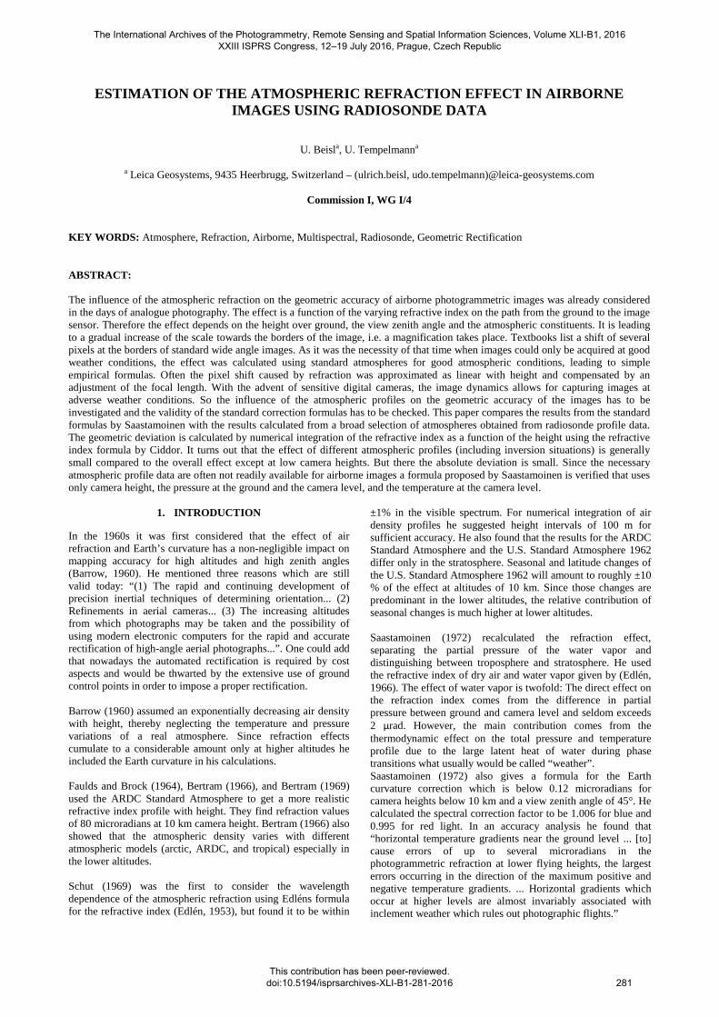
The basic set of data that is provided by a weather balloon is pressure, temperature and relative humidity as a function of the altitude. This data set is obtained at irregular altitude intervals depending on the vertical speed of the balloon. In order to get a periodic snapshot of the world atmosphere weather balloons are released at 00 UTC and 12 UTC all over the world. Appropriate data was selected to contain enough points for direct integration without additional modelling. The radiosonde profiles used also contained the dew point and the precipitable water column (Oolman, 2016). Radiosonde profiles with relative humidity above 98% at any elevation, as well as profiles where the temperature and the dew point were too close were skipped in order to avoid hazy or rainy situations which are not a realistic scenario for photogrammetric image flights. A Skew-T Log-P emagram helped to perform this task (Figure 1). 3.2 Selection Criteria for the Radiosonde Sites

As a first guide line for the selection of the stations in (Table 1) was the set of atmosphere types that are distinguished by the MODTRAN radiation transfer software. The atmospheres were:

US Standard 1976, tropical 15° N, mid latitude summer (mls) 45° N, mid latitude winter (mlw) 45° N, subarctic summer (ss) 60° N and subarctic winter (sw) 60° N. The sites were chosen such that the actual water column matched to the water column value of the model atmosphere in order to get a typical data set. For subartic summer and subarctic winter an inland site (Jokioinen) and an island site (Lerwick/Shetland) was chosen. The tropical site was tested for two seasons (February and September and an additional day – February 3rd - which probably was very hazy). The Tucson site was chosen to observe seasonal effects. Finally, four sites with high altitudes were selected (Nagqu, Lhasa, Flagstaff, and Tucson) to find any systematics in case of low camera height above ground.

Figure 1. A Skew-T Log-P diagram of the radiosonde profile at Tucson AZ on Jan 4 2015, 00 UTC. The temperature profile (right) is clearly separated from the dew point curve (left). The x axis is the temperature in °C and skewed by an angle of 45° as indicated by the straight blue lines in the grid in order to make the plot more compact. The inverse logarithmic y axis is the air pressure in mbar, corresponding to an approximately linear height over ground scale as indicated at the horizontal grid lines. The water column (PWAT) was 7.94 mm = 0.794 g/cm2. The temperature profile is showing an inversion (rising temperature with increasing altitude, indicated by a red ellipse) between 1500 m and 2000 m. This stable zone is separating a calm ground layer from a turbulent upper layer (cf. the feathered arrows on the right side).

WMO-ID

Latitude [°]

Longitude [°]

Elevation [m]

Description State Date [dd.mm.yyyy]

Time UTC [hh]

Time Zone

Model Atmosphere

Model water [mm]

Sonde water [mm]

55299 31.48 92.07 4508 Nagqu CI 20.06.2015 12 8 US 1976 11.2 7.22 55591 29.67 91.13 3650 Lhasa CI 15.06.2015 12 8 US 1976 11.2 10.45 72376 35.23 -111.82 2180 Flgstf/Belemont AZ/US 15.06.2015 0 -7 US 1976 11.2 16.72 72274 32.12 -110.93 779 Tucson Intl Airport AZ/US 15.06.2015 0 -7 US 1976 11.2 15.61 48698 1.37 103.98 16 Singapore/Changi SR 15.02.2015 12 8 trop 15° N 32.3 41.86 10771 49.43 11.9 419 Kümmersbruck DL 12.07.2015 12 1 mls 45° N 23.6 23.95 48698 1.37 103.98 16 Singapore/Changi SR 03.09.2015 12 8 trop 15° N 32.3 53.1 48698 1.37 103.98 16 Singapore/Changi SR 03.02.2015 12 8 trop 15° N 32.3 57.63 2963 60.82 23.5 103 Jokioinen FI 15.07.2015 12 1 ss 60° N 16.5 18.04 10771 49.43 11.9 419 Kümmersbruck DL 20.02.2015 12 1 mlw 45° N 6.9 6.85 2963 60.82 23.5 103 Jokioinen FI 15.02.2015 12 1 sw 60° N 3.3 2.17 3005 60.13 -1.18 82 Lerwick/Shetland UK 02.06.2015 12 0 ss 60° N 16.5 11.89 3005 60.13 -1.18 82 Lerwick/Shetland UK 02.02.2015 12 0 sw 60° N 3.3 89.93 Table 1. Radiosonde sites sorted by increasing refractive displacement at 10 km camera height.



283

4. CALCULATIONS AND COMPARISON

4.1 Comparison of different refraction formulas

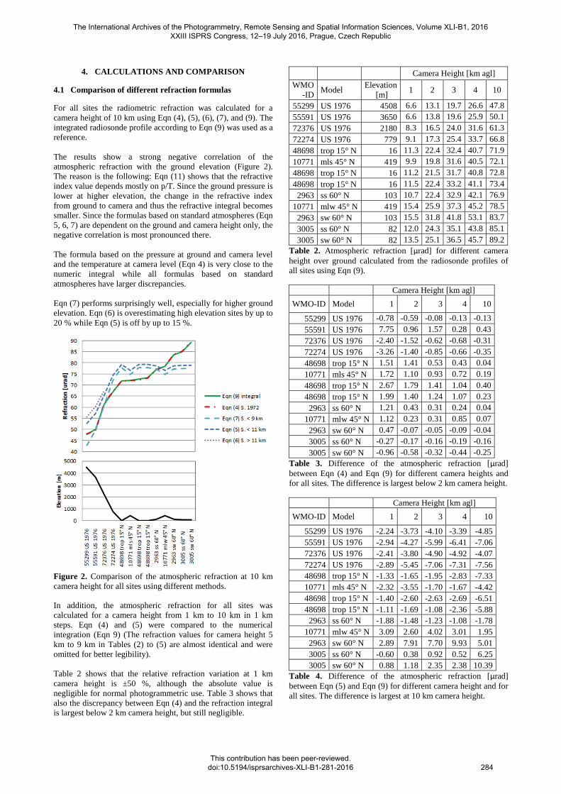
For all sites the radiometric refraction was calculated for a camera height of 10 km using Eqn (4), (5), (6), (7), and (9). The integrated radiosonde profile according to Eqn (9) was used as a reference. The results show a strong negative correlation of the atmospheric refraction with the ground elevation (Figure 2). The reason is the following: Eqn (11) shows that the refractive index value depends mostly on p/T. Since the ground pressure is lower at higher elevation, the change in the refractive index from ground to camera and thus the refractive integral becomes smaller. Since the formulas based on standard atmospheres (Eqn 5, 6, 7) are dependent on the ground and camera height only, the negative correlation is most pronounced there. The formula based on the pressure at ground and camera level and the temperature at camera level (Eqn 4) is very close to the numeric integral while all formulas based on standard atmospheres have larger discrepancies. Eqn (7) performs surprisingly well, especially for higher ground elevation. Eqn (6) is overestimating high elevation sites by up to 20 % while Eqn (5) is off by up to 15 %.

Figure 2. Comparison of the atmospheric refraction at 10 km camera height for all sites using different methods.

In addition, the atmospheric refraction for all sites was calculated for a camera height from 1 km to 10 km in 1 km steps. Eqn (4) and (5) were compared to the numerical integration (Eqn 9) (The refraction values for camera height 5 km to 9 km in Tables (2) to (5) are almost identical and were omitted for better legibility). Table 2 shows that the relative refraction variation at 1 km camera height is ±50 %, although the absolute value is negligible for normal photogrammetric use. Table 3 shows that also the discrepancy between Eqn (4) and the refraction integral is largest below 2 km camera height, but still negligible.

Camera Height [km agl] WMO

-ID Model

Elevation [m]

1 2 3 4 10

55299 US 1976 4508 6.6 13.1 19.7 26.6 47.8 55591 US 1976 3650 6.6 13.8 19.6 25.9 50.1 72376 US 1976 2180 8.3 16.5 24.0 31.6 61.3 72274 US 1976 779 9.1 17.3 25.4 33.7 66.8 48698 trop 15° N 16 11.3 22.4 32.4 40.7 71.9 10771 mls 45° N 419 9.9 19.8 31.6 40.5 72.1 48698 trop 15° N 16 11.2 21.5 31.7 40.8 72.8 48698 trop 15° N 16 11.5 22.4 33.2 41.1 73.4 2963 ss 60° N 103 10.7 22.4 32.9 42.1 76.9

10771 mlw 45° N 419 15.4 25.9 37.3 45.2 78.5 2963 sw 60° N 103 15.5 31.8 41.8 53.1 83.7 3005 ss 60° N 82 12.0 24.3 35.1 43.8 85.1 3005 sw 60° N 82 13.5 25.1 36.5 45.7 89.2

Table 2. Atmospheric refraction [μrad] for different camera height over ground calculated from the radiosonde profiles of all sites using Eqn (9).

Camera Height [km agl]

WMO-ID Model 1 2 3 4 10

55299 US 1976 -0.78 -0.59 -0.08 -0.13 -0.13 55591 US 1976 7.75 0.96 1.57 0.28 0.43 72376 US 1976 -2.40 -1.52 -0.62 -0.68 -0.31 72274 US 1976 -3.26 -1.40 -0.85 -0.66 -0.35 48698 trop 15° N 1.51 1.41 0.53 0.43 0.04 10771 mls 45° N 1.72 1.10 0.93 0.72 0.19 48698 trop 15° N 2.67 1.79 1.41 1.04 0.40 48698 trop 15° N 1.99 1.40 1.24 1.07 0.23 2963 ss 60° N 1.21 0.43 0.31 0.24 0.04

10771 mlw 45° N 1.12 0.23 0.31 0.85 0.07 2963 sw 60° N 0.47 -0.07 -0.05 -0.09 -0.04 3005 ss 60° N -0.27 -0.17 -0.16 -0.19 -0.16 3005 sw 60° N -0.96 -0.58 -0.32 -0.44 -0.25

Table 3. Difference of the atmospheric refraction [μrad] between Eqn (4) and Eqn (9) for different camera heights and for all sites. The difference is largest below 2 km camera height.



55299 US 1976 -2.24 -3.73 -4.10 -3.39 -4.85 55591 US 1976 -2.94 -4.27 -5.99 -6.41 -7.06 72376 US 1976 -2.41 -3.80 -4.90 -4.92 -4.07 72274 US 1976 -2.89 -5.45 -7.06 -7.31 -7.56 48698 trop 15° N -1.33 -1.65 -1.95 -2.83 -7.33 10771 mls 45° N -2.32 -3.55 -1.70 -1.67 -4.42 48698 trop 15° N -1.40 -2.60 -2.63 -2.69 -6.51 48698 trop 15° N -1.11 -1.69 -1.08 -2.36 -5.88 2963 ss 60° N -1.88 -1.48 -1.23 -1.08 -1.78

10771 mlw 45° N 3.09 2.60 4.02 3.01 1.95 2963 sw 60° N 2.89 7.91 7.70 9.93 5.01 3005 ss 60° N -0.60 0.38 0.92 0.52 6.25 3005 sw 60° N 0.88 1.18 2.35 2.38 10.39

Table 4. Difference of the atmospheric refraction [μrad] between Eqn (5) and Eqn (9) for different camera height and for all sites. The difference is largest at 10 km camera height.



284



55299 US 1976 -0.18 -0.31 -0.34 -0.28 -0.40 55591 US 1976 -0.24 -0.35 -0.49 -0.52 -0.58 72376 US 1976 -0.20 -0.31 -0.40 -0.40 -0.33 72274 US 1976 -0.24 -0.45 -0.58 -0.60 -0.62 48698 trop 15° N -0.11 -0.13 -0.16 -0.23 -0.60 10771 mls 45° N -0.19 -0.29 -0.14 -0.14 -0.36 48698 trop 15° N -0.11 -0.21 -0.22 -0.22 -0.53 48698 trop 15° N -0.09 -0.14 -0.09 -0.19 -0.48 2963 ss 60° N -0.15 -0.12 -0.10 -0.09 -0.15

10771 mlw 45° N 0.25 0.21 0.33 0.25 0.16 2963 sw 60° N 0.24 0.65 0.63 0.81 0.41 3005 ss 60° N -0.05 0.03 0.08 0.04 0.51 3005 sw 60° N 0.07 0.10 0.19 0.19 0.85

Table 5. Difference of the radial image height displacement [um] between Eqn (5) and Eqn (9) for different camera height and for all sites for a camera with a view angle of ±38° and a focal length of 62.7 mm.

In contrast, Eqn (5), using a standard atmosphere, has a stronger discrepancy below 2 km camera height than Eqn (4) and it even increases with camera height (Table 4). The radial displacement in the focal plane for a camera with a view angle of ±38° and a focal length of 62.7 mm stays below a fifth of a pixel (Table 5). 4.2 Influence of the atmosphere

Figure 3. Refraction for different spectral colors at 10 km camera height vs. water column.

For all sites the radiometric refraction was calculated for a camera height of 10 km using Eqn (9) and the Ciddor formula for the refractive index evaluated at four spectral wavelengths (465 nm, 555 nm, 635 nm, and 845nm). As already stated by Schut (1969), the spectral variation of the atmospheric refraction is negligible for practical purposes (Figure 3). Although the atmospheric refraction also showed no apparent correlation with the water column (Figure 3) the variation is considerable: Compared to a midlatitude summer atmosphere the refraction value at 10 km camera height dropped by 34% at a 4500 m elevation site and increased by 24 % at a subarctic summer site. As stated already in sec. (4.1) high elevation sites have a smaller refraction integral. On the other hand, Saastamoinen (1974) mentioned that subarctic sites have a

higher sea-level pressure and a lower sea-level temperature than tropical sites, which leads to a higher p/T value and hence a higher refractivity index at the ground level (Eqn 11) and consequently to a higher refraction integral. 4.3 Seasonal changes in refraction

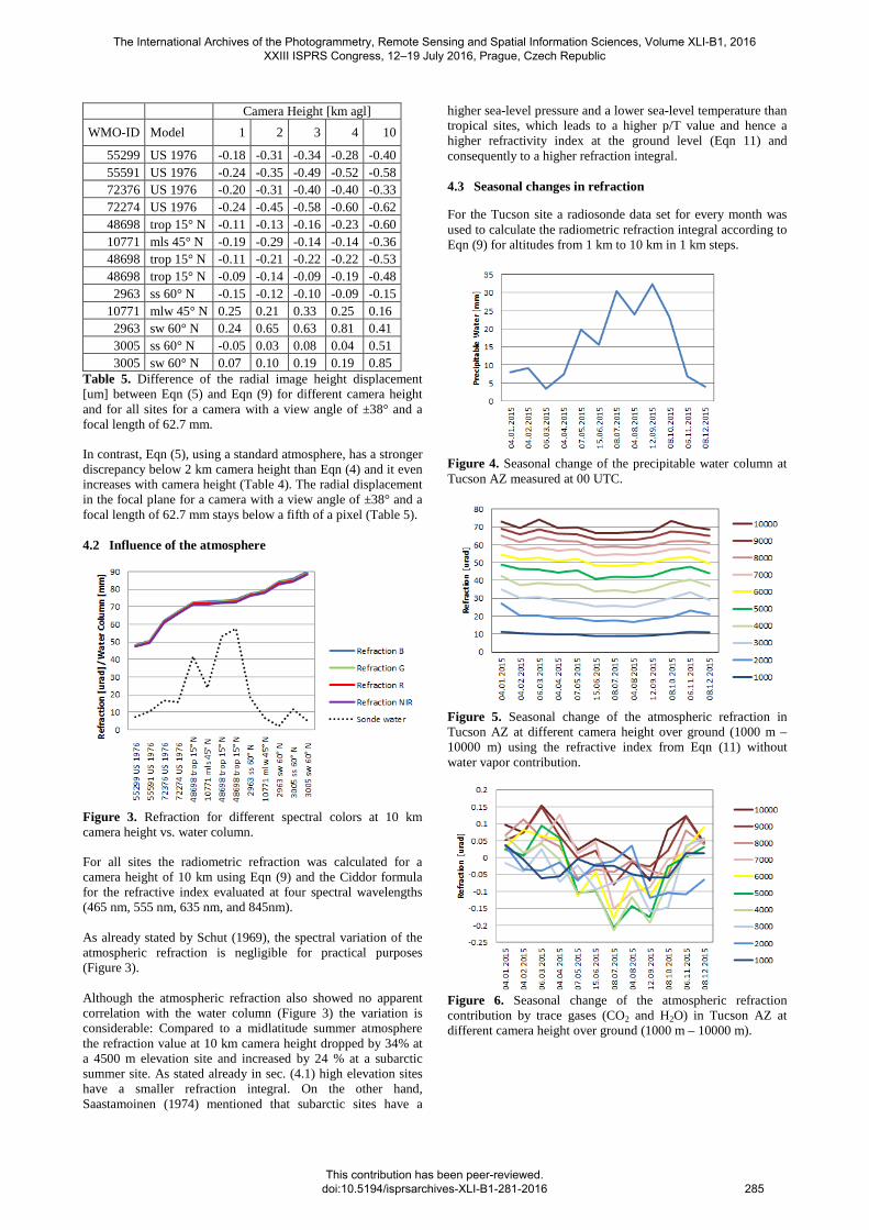
For the Tucson site a radiosonde data set for every month was used to calculate the radiometric refraction integral according to Eqn (9) for altitudes from 1 km to 10 km in 1 km steps.

Figure 4. Seasonal change of the precipitable water column at Tucson AZ measured at 00 UTC.

Figure 5. Seasonal change of the atmospheric refraction in Tucson AZ at different camera height over ground (1000 m – 10000 m) using the refractive index from Eqn (11) without water vapor contribution.

Figure 6. Seasonal change of the atmospheric refraction contribution by trace gases (CO2 and H2O) in Tucson AZ at different camera height over ground (1000 m – 10000 m).



285

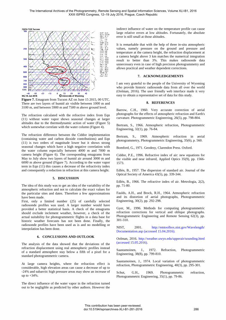
Figure 7. Emagram from Tucson AZ on June 15 2015, 00 UTC. There are two layers of humid air visible between 1000 m and 3100 m, and between 5900 m and 7500 m above ground level.

The refraction calculated with the refractive index from Eqn (11) without water vapor shows seasonal changes at larger altitudes due to the thermodynamic action of water (Figure 5) which somewhat correlate with the water column (Figure 4). The refraction difference between the Ciddor implementation (containing water and carbon dioxide contributions) and Eqn (11) is two orders of magnitude lower but it shows strong seasonal changes which have a high negative correlation with the water column especially between 4000 m and 7000 m camera height (Figure 6). The corresponding emagrams from May to July show two layers of humid air around 3000 m and 6000 m above ground (Figure 7). According to the water vapor term in Eqn (11) this causes a decrease of the refractivity index and consequently a reduction in refraction at this camera height.

5. DISCUSSION

The idea of this study was to get an idea of the variability of the atmospheric refraction and not to calculate the exact values for the particular sites and dates. Therefore a few approximations have been made. First, only a limited number (25) of carefully selected radiosonde profiles was used. A larger number would have provided a better statistical basis. A check of the emagrams should exclude inclement weather, however, a check of the actual suitability for photogrammetric flights in a data base for historic weather forecasts has not been done. Finally, the radiosonde profiles have been used as is and no modelling or interpolation has been done.

6. CONCLUSIONS AND OUTLOOK

The analysis of the data showed that the deviations of the refraction displacement using real atmospheric profiles instead of a standard atmosphere stay below a fifth of a pixel for a standard photogrammetric camera. At large camera heights, where the refraction effect is considerable, high elevation areas can cause a decrease of up to -24% and subarctic high pressure areas may show an increase of up to +34%. The direct influence of the water vapor in the refraction turned out to be negligible as predicted by other authors. However the

indirect influence of water on the temperature profile can cause large relative errors at low altitudes. Fortunately, the absolute error is still small at those altitudes. It is remarkable that with the help of three in-situ atmospheric values, namely pressure on the ground and pressure and temperature at the camera height, the refraction displacement at a camera height above 3 km matches the numerical integration result to better than 3%. This makes radiosonde data unnecessary even in case of high precision photogrammetry and allows practical and weather dependent corrections.

7. ACKNOWLEDGEMENTS

I am very grateful to the people of the University of Wyoming who provide historic radiosonde data from all over the world (Oolman, 2016). The user friendly web interface made it very easy to obtain a representative set of data for this study.

8. REFERENCES

Barrow, C.H., 1960. Very accurate correction of aerial photographs for the effects of atmospheric refraction and Earth's curvature. Photogrammetric Engineering, 26(5), pp. 798-804.

Bertram, S., 1966. Atmospheric refraction, Photogrammetric Engineering, 32(1), pp. 76-84.

Bertram, S., 1969. Atmospheric refraction in aerial photogrammetry, Photogrammetric Engineering, 35(6), p. 560.

Bomford, G., 1971. Geodesy, Clarendon Press. Oxford.

Ciddor, P.E., 1996. Refractive index of air: new equations for the visible and near infrared, Applied Optics 35(9), pp. 1566-1573.

Edlén, B., 1957. The dispersion of standard air. Journal of the Optical Society of America 43(5), pp. 339-344.

Edlén, B., 1966. The refractive index of air. Metrologia, 2(2), pp. 71-80.

Faulds, A.H., and Brock, R.H., 1964. Atmospheric refraction and its distortion of aerial photographs, Photogrammetric Engineering, 30(2), pp. 292-298.

Gyer, M., 1996. Methods for computing photogrammetric refraction corrections for vertical and oblique photographs. Photogrammetric Engineering and Remote Sensing 62(3), pp. 301-310.

NIST, 2001. http://emtoolbox.nist.gov/Wavelength/ Documentation.asp (accessed 15.04.2016).

Oolman, 2016. http://weather.uwyo.edu/upperair/sounding.html (accessed 15.05.2016).

Saastamoinen, J., 1972. Refraction, Photogrammetric Engineering, 38(8), pp. 799-810.

Saastamoinen, J., 1974. Local variation of photogrammetric refraction, Photogrammetric Engineering, 40(3), pp. 295-301.

Schut, G.H., 1969. Photogrammetric refraction, Photogrammetric Engineering, 35(1), pp. 79-86.



286

estimation of the atmospheric refraction ......estimation of the atmospheric refraction effect in...

Documents