Ps

Ma

b

c

d

a

ARRA

KDCCCMS

P

h1

Europ. J. Agronomy 76 (2016) 41–53

Contents lists available at ScienceDirect

European Journal of Agronomy

journa l homepage: www.e lsev ier .com/ locate /e ja

erformance and sensitivity of the DSSAT crop growth model inimulating maize yield under conservation agriculture

arc Corbeels a,b,∗, Guillaume Chirat a, Samir Messad c, Christian Thierfelder d

CIRAD, AIDA (Agro-ecology and Sustainable Intensification of Annual Crops), Av. Agropolis, 34060 Montpellier, FranceCIMMYT, SIP (Sustainable Intensification Program), P.O. Box 1041-00621, Gigiri, Nairobi, KenyaCIRAD, SELMET (Mediterranean and tropical livestock systems), Av. Agropolis, 34060 Montpellier, FranceCIMMYT, SIP (Sustainable Intensification Program), P.O. Box MP 163, Mount Pleasant, Harare, Zimbabwe

r t i c l e i n f o

rticle history:eceived 19 May 2015eceived in revised form 3 February 2016ccepted 7 February 2016

eywords:SSATo-inertia analysisonservation agriculturerop growth modelaize

ensitivity analysis

a b s t r a c t

With the practice of conservation agriculture (CA) soil water and nutrient dynamics are modified by thepresence of a mulch of crop residues and by reduced or no-tillage. These alterations may have impactson crop yields. The crop growth model DSSAT (Decision Support Systems for Agrotechnology Transfer)has recently been modified and used to simulate these impacts on crop growth and yield. In this study,we applied DSSAT to a long-term experiment with maize (Zea mays L.) grown under contrasting tillageand residue management practices in Monze, Southern Province of Zambia. The aim was (1) to assess thecapability of DSSAT in simulating crop responses to mulching and no-tillage, and (2) to understand thesensitivity of DSSAT model output to input parameters, with special attention to the determinants of themodel response to the practice of CA. The model was first parameterized and calibrated for the tillagetreatment (CP) of the experiment, and then run for the CA treatment by removing tillage and applyinga mulch of crop residues in the model. In order to reproduce observed maize yields under the CP versusCA treatment, optimal root development in the model was restricted to the upper 22 cm soil layer inthe CP treatment, while roots could optimally develop to 100 cm depth under CA. The normalized RMSEvalues between observed and simulated maize phenology and total above ground biomass and grainyield indicated that the CA treatment was equally well simulated as the CP treatment, for which themodel was calibrated. A global sensitivity analysis using co-inertia analysis was performed to describethe DSSAT model response to 32 model input parameters and crop management factors. Phenologicalcultivar parameters were the most influential model parameters. This analysis also demonstrated thatin DSSAT mulching primarily affects the surface soil organic carbon content and secondly the total soilmoisture content, since it is negatively correlated with simulated soil water evaporation and run-off. Thecorrelations between the input parameters or crop management factors and the output variables werestable over a wide range of seasonal rainfall conditions. A local sensitivity analysis of simulated maizeyield to three key parameters for the simulation of the CA practice revealed that DSSAT responds tomulching particularly when rooting depth is restricted, i.e., when water is a critical limiting crop growth

factor. The results of this study demonstrate that DSSAT can be used to simulate crop responses to CA,in particular through simulated mulching effects on the soil water balance, but other, often site-specific,factors that are not modeled by DSSAT, such as plough pan formation under CP or improved soil structureunder CA, may need to be considered in the model parameterization to reproduce the observed crop yieldeffects of CA versus CP.

© 2016 Elsevier B.V. All rights reserved.

∗ Corresponding author at: CIMMYT, SIP (Sustainable Intensification Program),.O. Box 1041-00621, Gigiri, Nairobi, Kenya.

E-mail address: marc.corbeels@cirad.fr (M. Corbeels).

ttp://dx.doi.org/10.1016/j.eja.2016.02.001161-0301/© 2016 Elsevier B.V. All rights reserved.

1. Introduction

Conservation agriculture (CA) is nowadays perceived as a setof best-management practices based on no-tillage, crop residue

mulching and the use of crop rotations and/or associations, throughwhich African agriculture can combat soil degradation, secure cropyields and mitigate to some extent negative effects of climatechange (Gowing and Palmer, 2008; Thierfelder et al., 2014), even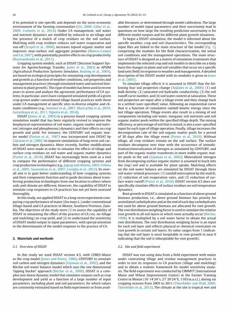

4 . J. Agr

ie2atMria(

t(aamtytcumG

sbegtGbos(tceaafsst

ptbDaot

2

2

asR‘pdpa

2 M. Corbeels et al. / Europ

f its potential is site-specific and depends on the socio-economicnvironment of the farming communities (Uri, 2000; Giller et al.,009; Corbeels et al., 2014). Under CA management, soil waternd nutrient dynamics are modified by reduced or no-tillage andhe presence of a mulch of crop residues on the soil surface.

ulching with crop residues reduces soil water evaporation andun-off (Scopel et al., 2004), increases topsoil organic matter andmproves near-surface soil aggregate properties (Blanco-Canquind Lal, 2007), with potentially positive effects on crop productivityRusinamhodzi et al., 2011).

Cropping system models, such as DSSAT (Decision Support Sys-ems for Agrotechnology Transfer, Jones et al., 2003) or APSIMAgricultural Production Systems Simulator, Keating et al., 2003),re based on ecological principles for simulating crop developmentnd growth as a function of weather conditions, soil properties andanagement practices (through simulated water and nutrient limi-

ations to plant growth). This type of models has been used in recentears to assess and analyze the agronomic performance of CA sys-ems. In particular, users have compared simulated yields of a givenrop grown under conventional tillage-based practices with thosender CA management at specific sites in diverse edaphic and cli-atic conditions (e.g., Sommer et al., 2007; MacCarthy et al., 2010;erardeaux et al., 2011; Ngwira et al., 2014).

DSSAT (Jones et al., 2003) is a process-based cropping systemimulation model that has been regularly revised to improve theiophysical representation of soil water, organic matter and nutri-nt (nitrogen and phosphorous) dynamics and their effects on croprowth and yield. For instance, the CENTURY soil organic mat-er model (Parton et al., 1987) was incorporated into DSSAT byijsman et al. (2002) to improve simulations of long-term soil car-on and nitrogen dynamics. More recently, further modificationsf DSSAT were made in order to simulate the effects of tillage andurface crop residues on soil water and organic matter dynamicsPorter et al., 2010). DSSAT has increasingly been used as a toolo compare the performance of different cropping systems androp production technologies (e.g., Jagtap and Abamu, 2003; Fofanat al., 2005; Saseendran et al., 2007; Caviglia et al., 2013). Its over-ll aim is to gain better understanding of how cropping systemsnd their components function and to guide decisions about trans-erring production technologies from one location to others whereoils and climate are different. However, the capability of DSSAT toimulate crop responses to CA practices has not yet been assessedhoroughly.

In this study, we applied DSSAT to a long-term experiment com-aring crop performance of maize (Zea mays L.) under conventionalillage-based and CA practices in Monze, Southern Province, Zam-ia. The objectives of the study were (1) to assess the capability ofSSAT in simulating the effect of the practice of CA (viz. no-tillagend mulching) on crop yield, and (2) to understand the sensitivityf DSSAT model output to input parameters, with special attentiono the determinants of the model response to the practice of CA.

. Materials and methods

.1. Overview of DSSAT

In this study we used DSSAT version 4.5, with CERES-Maizes the crop model (Jones and Kiniry, 1986), CENTURY to simulateoil carbon and nitrogen dynamics (Gijsman et al., 2002), and theitchie soil water balance model which uses the one dimensional

tipping bucket’ approach (Ritchie et al., 2009). DSSAT is a com-

lex non-linear dynamic model that simulates outputs such as cropevelopment and yield as a function of a large number of inputarameters, including plant and soil parameters, for which valuesre commonly estimated based on field experiments or from avail-

onomy 76 (2016) 41–53

able literature, or determined through model calibration. The largenumber of model input parameters and their uncertainty lead toquestions on how large the resulting prediction uncertainty is fordifferent model outputs and for different plant growth situations.

To begin a DSSAT simulation, the model is informed about thespecific weather, crop and soil characteristics. The correspondinginput files are linked to the main structure of the model (Fig. 1),comprising the modules for the field characterization, the initialsoil conditions and the management operations. The main struc-ture of DSSAT is designed as a matrix of simulation treatments thatimplements the selected crop and soil models to describe on a dailybasis the changes in plant and soil variables that occur on a specificland unit (field) in response to weather and management. A detaileddescription of the DSSAT model with its modules is given in Joneset al. (2003).

To simulate tillage effects it is assumed in DSSAT that the fol-lowing four soil properties change (Andales et al., 2000): (1) soilbulk density; (2) saturated soil hydraulic conductivity; (3) the soilrunoff curve number, and (4) soil water content at saturation. Thesesoil properties are input after a tillage event and they change backto a settled (user-specified) value, following an exponential curvethat is a function of cumulative rainfall kinetic energy since thelast tillage operation. Tillage events also result in a mixing of soilcomponents including soil water, inorganic soil nutrients and soilorganic matter pools within the specified tillage depth. The mixingefficiency, or percentage of soil that is mixed, is also a user-specifiedinput for each type of tillage operation. Finally, tillage increases thedecomposition rate of the soil organic matter pools for a periodof 30 days after the tillage event (Porter et al., 2010). Withouttillage, all crop residues remain on the soil surface. The surfaceresidues decompose over time with the occurrence of immobi-lization/mineralization of nitrogen as simulated by CENTURY, andpart of the organic matter transforms in more stable organic mat-ter pools in the soil (Gijsman et al., 2002). Mineralized nitrogenfrom decomposing surface organic matter is assumed to leach intothe (top) soil and is available for plant uptake. Mulching effectson the soil water balance are simulated by DSSAT through threesoil water-related processes: (1) rainfall interception by the mulch;(2) reduction of soil evaporation rates, and (3) reduction of sur-face water runoff (Porter et al., 2010). DSSAT version 4.5 does notspecifically simulate effects of surface residues on soil temperaturedynamics.

Root growth in DSSAT is simulated as a function of above groundbiomass production, i.e., above ground biomass has priority forassimilated carbohydrates and at the end of each day carbohydratesnot used for above ground biomass are allocated for root growth.The root distribution weighing factor is used to simulate the relativeroot growth in all soil layers in which roots actually occur (Ritchie,1998). It is multiplied by a soil water factor to obtain the actualroot distribution. The root distribution weighing factor is an inputfor each soil layer and reflects physical or chemical constraints onroot growth in certain soil layers. Its value ranges from 1 (indicat-ing that the soil layer is most hospitable to root growth to near 0indicating that the soil is inhospitable for root growth).

2.2. Site and field experiment

DSSAT was run using data from a field experiment with maizeunder contrasting tillage and residue management practices inorder to test its responses to CA practices (tillage and mulching)and to obtain a realistic framework for model sensitivity analy-sis. The field experiment was conducted by CIMMYT (International

Maize and Wheat Improvement Centre) at the Farmer TrainingCentre in Monze (16◦14′24′′s, 27◦26′24′′E, 1103 m.a.s.l.), during sixcropping seasons from 2005 to 2011 (Thierfelder and Wall, 2009;Thierfelder et al., 2013). The climate at the site is tropical wet and

M. Corbeels et al. / Europ. J. Agronomy 76 (2016) 41–53 43

Fig. 1. Overview of the components and modular structure of the DSSAT model.

Table 1Values of soil parameters of the soil module of DSSAT for the maize experiment in Monze, Zambia.

Soil layer (cm) Albedo Soilevapora-tion limit(mm)

Drainagerate(day−1)

Runoffcurvenumber

surface 0.14 3 0.75 84

Clay (%) Silt (%) Organic C(%)

pH in water CEC(cmol kg−1)

Bulkdensity(g cm−3)

Crop-determinedlower limit(cm3 cm−3)

Drained upperlimit(cm3 cm−3)

Saturatedupper limit(cm3 cm−3)

Hydraulicconductivity(cm h−1)

0–22 16 5 0.6 4.4 3.1 1.67 0.122 0.187 0.38 2.623–56 37 8 0.3 5.1 4.0 1.48 0.228 0.314 0.40 0.4

1.41.31.4

dpattwswst

c

57–80 38 8 0.05 5.3 5.3

81–107 44 7 0.05 5.6 5.4

>–107 43 7 0.05 5.7 6.7

ry (Aw, Köppen Climate Classification) with a unimodal rainfallattern (Fig. 2). Rains start in November and end in April. Theverage annual rainfall at the site is 750 mm. During the dura-ion of the experiment, four seasons had normal rainfall, whilsthe 2006/2007 season was drier (510 mm) and that of 2007/2008as wetter (1000 mm) than normal. The soil at the experimental

ite is a ferric Lixisol (Thierfelder and Wall, 2009). Five soil profilesere characterized on the experimental site as a variation of the

ame soil type. For the model simulations we considered the mostypical soil profile for the site, as described in Table 1.

From ten experimental treatments that were set up in 2005, twoontrasting treatments were selected for the model simulations:

8 0.264 0.309 0.39 0.13 0.296 0.331 0.39 0.18 0.304 0.324 0.39 0.1

the conventional tillage (using a moldboard plough) treatment (CP)with removal of the crop harvest residues, and the CA treatment(CA) with the use of an animal traction direct seeder and cropresidue mulching. Maize was sown between late November andearly December with a target population of 44 000 plants ha−1. Thecommercial hybrid maize variety SC513 was used in 2005/2006and 2006/2007, thereafter it was replaced with the variety MRI624.Both are early to medium maturing varieties. Basal fertiliza-

−1

tion was carried out with 165 kg ha of Compound D (10:20:10,N:P2O5:K2O) at planting and 200 kg ha−1 urea (46% N) was appliedas top-dressing in a split application, five to seven weeks afterplanting. Weed control was done by a pre-emergence application of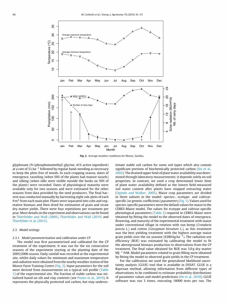

44 M. Corbeels et al. / Europ. J. Agronomy 76 (2016) 41–53

condit

gateatasv9edyiT

2

2

ts2saMw1tr

Fig. 2. Average weather

lyphosate (N-(phosphonomethyl) glycine, 41% active ingredient)t a rate of 3 L ha−1 followed by regular hand-weeding as necessaryo keep the plots free of weeds. In each cropping season, dates ofmergence, tasseling (when 50% of the plants had mature tassels)nd silking (when silks were visible outside the husks on 50% ofhe plants) were recorded. Dates of physiological maturity werevailable only for two seasons and were estimated for the othereasons from data provided by the seed producers. The final har-est was conducted manually by harvesting eight sub-plots of each

m2 from each main plot. Plants were separated into cobs and veg-tative biomass and then dried for estimation of grain and strawry matter yields. There were four repetitions per treatment perear. More details on the experiment and observations can be foundn Thierfelder and Wall (2009), Thierfelder and Wall (2010) andhierfelder et al. (2013).

.3. Model settings

.3.1. Model parameterisation and calibration under CPThe model was first parameterised and calibrated for the CP

reatment of the experiment. It was run for the six consecutiveeasons of the experiment starting at the planting date of the005/2006 season. Daily rainfall was recorded at the experimentalite, whilst daily values for minimum and maximum temperaturend radiation were obtained from the nearby weather station of theonze Farm Training Centre (Fig. 2). Input parameters for the soil

ere derived from measurements on a typical soil profile (Table

) of the experimental site. The fraction of stable carbon was ini-ialized based on silt and clay contents (see Porter et al., 2010). Itepresents the physically protected soil carbon, but may underes-

ions for Monze, Zambia.

timate stable soil carbon for some soil types which also containsignificant portions of biochemically protected carbon (Six et al.,2002). The drained upper limit of plant water availability was deter-mined through laboratory measurements; it depends solely on soilproperties. In contrast, we used a crop determined lower limitof plant water availability defined as the lowest field-measuredsoil water content after plants have stopped extracting water(Ogindo and Walker, 2005). Maize crop parameters are dividedin three subsets in the model: species-, ecotype- and cultivar-specific (or genetic coefficients) parameters (Fig. 1). Values used forspecies-specific parameters were the default values for maize in theCERES-Maize model. The values for ecotype and cultivar-specificphenological parameters (Table 2) required in CERES-Maize wereobtained by fitting the model to the observed dates of emergence,flowering, and maturity of the experimental treatment with maizeunder conventional tillage in rotation with sun hemp (Crotalariajuncea L.) and cotton (Gossypium hirsutum L.), as this treatmentwas the best yielding treatment with the highest average maizegrain yields over the six seasons (6380 kg ha−1). The radiation useefficiency (RUE) was estimated by calibrating the model to fitthe aboveground biomass production to observations from the CPtreatment. The final value obtained for RUE was 3.0 g dry matterMJ−1 PAR. Model parameters related to grain filling were obtainedby fitting the model to observed grain yields in the CP treatment.

For the calibration we used the generalized likelihood uncer-tainty analysis (GLUE) tool that is available in DSSAT. GLUE is a

Bayesian method, allowing information from different types ofobservations to be combined to estimate probability distributionsof parameter values and model predictions (He et al., 2010). GLUEsoftware was run 3 times, executing 18000 tests per run. The

M. Corbeels et al. / Europ. J. Agronomy 76 (2016) 41–53 45

Table 2Values of maize cultivar parameters as calibrated in the CERES-Maize crop model of DSSAT for the maize experiment in Monze, Zambia.

Cultivar P1 (◦C day) P2 (days) P5 (◦C days) G2 (number) G3 (mg day−1) PHINT (◦C day)

SC513 240 0.0 770 550 9 55MRI624 260 0.0 500 950 9 65

P1: Thermal time from seedlings emergence to the end of the juvenile phase (expressed in ◦C day, above a base temperature of 8 ◦C) during which the plant is not responsiveto changes in photoperiod. P2: Extent to which development (expressed as days) is delayed for each hour increase in photoperiod above the longest photoperiod at whichd Thermt fillingP essive

fmMrpao

tvttvmsa(clIttrld

2

totwsvfa3forD6ibo

2

tmc2ts

evelopment proceeds at a maximum rate (which is considered to be 12.5 h). P5:emperature of 8 ◦C). G2: Maximum possible number of kernels per plant. G3: KernelHINT: Phyllochron interval, i.e., the interval in thermal time (◦C day) between succ

ollowing variables were fitted: dates of emergence, flowering andaturity, grain yield and total above ground biomass at maturity.odel performance was evaluated by calculating the normalized

oot mean square error (RMSE), expressed in percentage, and theercentage prediction deviation. Calibration was considered aschieved when the RMSE for all fitted maize phenology and yieldutput variables was minimal.

An important feature under the CP treatment was the exis-ence of a plough pan, as suggested by the higher bulk densityalues in the 22–25 cm soil layer (unpublished data) comparedo the 0–22 cm soil layer. This plough plan restricts the pene-ration of roots of maize plants into deeper layers, which wasisually observed in the experiment. In contrast, in the CA treat-ent the plough plan had disappeared rapidly over time and the

oil developed a better soil structure with cracks and voids, which isttributed to greater soil biological activity (e.g., more earthworms)Thierfelder et al., 2013). The importance of this phenomenon forrop growth on similar soils in the region has already been high-ighted in other studies (e.g., Materechera and Mloza-Banda, 1997).n order to reproduce this effect of soil tillage in the model simula-ions, optimal root development rate was restricted in the model tohe upper 22 cm soil layer in the CP treatment, i.e., we reduced theoot distribution weighing factor by 80% (from 1 to 0.2) for the soilayers deeper than 22 cm resulting in restricted root growth overepth.

.3.2. Model testing for CAWe then ran the model for the CA treatment by turning off the

illage module in DSSAT, restoring the normal root developmentver soil depth, i.e., resetting the root distribution weighing fac-or equal to 1 over the whole soil depth, and initializing DSSATith a mulch of crop residues with resulting modeled effects on

oil properties and processes. Simulated biomass and grain yieldalues were then compared with observed values and model per-ormance was calculated as described for the CP treatment. Themounts of maize surface residues set in the CA simulations were000, 2300, 1300, 4000, 2700, 850 kg dry matter ha−1 at plantingrom 2005 to 2010. Values were estimated from the percentagef observed soil cover in the experiment. The C:N ratio of maizeesidues is a user-specified input value in DSSAT and was set at 60.epending on the initial amounts of residues it represents between

and 30 kg N ha−1. Part of this organic nitrogen is mineralized dur-ng the growing season (simulated by the CENTURY module) andecomes available as inorganic nitrogen for the crop. Values for allther model parameters were kept the same for CP and CA.

.4. Sensitivity analyses

First, a global sensitivity analysis was performed to describehe DSSAT model response to 32 model input parameters and crop

anagement factors (see Table 3). In this analysis simulations were

onducted under ‘normal’ rainfall conditions of Monze (i.e., the009/2010 season) with the experimental field characteristics ofhat season: planting date was 19th November; plant density waset at 44 000 plants ha−1. Second, we analyzed the effects of rainfall

al time from silking to physiological maturity (expressed in ◦C day above a base rate during the linear grain filling stage and under optimum conditions (mg day−1).

leaf tip appearances.

on the stability of the correlations between the input parameters orcrop management factors and the output variables through modelsimulations for a drier (2006/2007) and wetter (2007/2008) season.Third, we determined the local sensitivity of simulated maize yieldto three key parameters/variables (i.e., stable soil carbon fraction,depth of optimal root growth and amount of surface crop residues)for the simulation of the CA practice (viz. no-tillage and mulching).In the sections below we describe the details of the performedsensitivity analyses.

2.4.1. Global sensitivity analysisFor the global sensitivity analysis, we used the Latin Hyper-

cube Sampling method as described by McKay et al. (1979). Thismethod ensures that the whole range of possible parameter val-ues is randomly sampled and that effects of interactions betweeninput parameters, between input parameters and crop manage-ment factors, and between crop management factors on modeloutput variables are taken into account (Pathak et al., 2007).

The following model input parameters and management factorswere chosen for the sensitivity analysis (Table 3): (1) a set of inputparameters associated with the crop cultivars, since these param-eters are usually determined under sub-optimal plant growthconditions, whilst in the model their values refer to non-limitinggrowth conditions; (2) a second set of model input parameters thatrelate to soil moisture properties, that are often not measured inthe field, but are inferred from laboratory measurements, whichmay cause a laboratory-scale related systematic bias; (3) third, fac-tors related to nitrogen management and parameters of the soilorganic matter module (CENTURY) were selected, because nitro-gen is considered as the main limiting nutrient for the site (andother nutrients are not considered in the model) and, moreoverthe absence of tillage under CA is assumed to affect the rate ofnitrogen mineralization; and (4) finally, we selected the amountand quality (lignin content) of crop residues as key input factorsfor simulating the potential effect of CA on crop yield as a resultof mulching. Boundary values of the ecotype- and cultivar-specificinput parameters were fixed to represent African maize cultivars(Table 3). Boundary values for the soil parameter values were set tocharacterise ferric Lixisols as described by CIMMYT (5 profiles, seeSection 2.2). The model’s sensitivity to soil available water capac-ity and soil organic carbon content was assessed for values for twosoil layers: the first layer of the top 22 cm and the second layerfrom 22 to 56 cm (see Table 1). Finally, the boundary values for thenitrogen and residue management factors were set according to thepractices adopted by the local farmers (recorded from householdsurveys) and those applied at the CIMMYT experiment in Monze. Intotal, we ran 1388 combinations of input parameters and manage-ment factors with R software (R Development Core Team, 2009).

The model’s sensitivity to the selected input parameters andcrop management factors was assessed by looking at a set of model

output variables that are listed in Table 4. Crop grain yield and totalabove ground biomass are the integrative outputs of the model sim-ulations, the other model outputs can be regarded as key variablesthat help in explaining simulated crop growth and yields.

46 M. Corbeels et al. / Europ. J. Agronomy 76 (2016) 41–53

Table 3Selected input parameters and crop management factors for the global sensitivity analysis of DSSA for the maize experiment in Monze, Zambia.

Module/Class Variable Acronym Unit Min Max Source

Genotype/ecotypes Radiation use efficiency (dry matter conversion) RUE g MJ−1 PAR 2 5 Lindquist et al. (2005)Light extinction coefficient KCAN – 0.45 0.90 APSIM + DSSATThermal time from silking to effective grain filling period DSGFT ◦C day 85 255 DSSAT (default value ± 50%)Thermal time per cm seed depth required for emergence GDDE ◦C day cm−1 4 9 DSSAT + CIMMYT

Genotype/cultivars Thermal time from emergence to end of juvenile phase P1 ◦C day 130 380 DSSAT (range of valuesfor African cultivars)+Jagtap and Abamu(2003)

Thermal time from silking to physiological maturity P5 ◦C day 600 1100Potential kernel number/plant G2 plant−1 400 1100Potential grain filling rate G3 mg day−1 4.0 11.5Phyllocron interval PHINT ◦C day 30 90

Soil description/surfacelayer

Soil evaporation limit SLU1 mm 3 12 DSSAT + CIMMYT +Gijsman et al. (2002)Drainage rate SLDR day−1 0.01 0.95

Runoff curve number SLRO – 61 94Soil description/firstsoil layer (0–22 cm)

Lower limit SLLL.22 cm3 cm−3 0.02 0.25Drained upper limit SDUL.22 cm3 cm−3 0.08 0.45Saturated upper limit SSAT.22 cm3 cm−3 0.3 0.6Bulk density SADM.22 g cm−3 0.8 1.8Total organic C SAOC.22 % 0.2 3.0Stable organic C SASC.22 % 60 90

Soil description/secondsoil layer (22–56 cm)

Lower limit SLLL.56 cm3 cm−3 0.02 0.25Drained upper limit SDUL.56 cm3 cm−3 0.08 0.45Saturated upper limit SSAT.56 cm3 cm−3 0.3 0.6Bulk density SADM.56 g cm−3 0.8 1.8Total organic C SAOC.56 % 0.1 1.0Stable organic C SASC.56 % 60 90

Main structure/initialconditions

Initial soil volumetric water content SH2O cm3 cm−3 0.0 0.3 CIMMYTInitial soil nitrate content SNO3 g N Mg−1 soil 0 10

Mainstructure/inorganicfertilizers

N at seeding (0 DAP*) FAMN.0 kg N ha−1 0 20 CIMMYTN at 30 DAP FAMN.30 kg N ha−1 0 50N at 50 DAP FAMN.50 kg N ha−1 0 50

Main structure/organicfertilizers

Amount of crop residues (dry matter) at planting RAMT kg ha−1 0 6000 CIMMYT + Waddingtonand Karigwindi (2004)Lignin content crop residues PSLIG (fraction) 0.05 0.20

N content crop residues SCN % 0.5 2.0

* DAP: days after planting.

Table 4Selected output parameters for the global sensitivity analysis of DSSAT for the maize experiment in Monze, Zambia.

Category Variable Unit Acronym

Crop growth anddevelopment

Grain yield kg ha−1 YieldVegetative above ground biomass (straw yield) kg ha−1 BiomLAI max – LaiMCumulative plant N uptake kg N ha−1 NupEmergence Days after planting EmerSilking Days after planting SilkMaturity Days after planting MatCumulative plant transpiration mm Transpi

Soil water Cumulative soil evaporation mm sEvapCumulative runoff mm RunTotal soil moisture at maturity mm sMoist

−1

tnuc(sr

aspambvy

Soil fertility Cumulative net N mineralization

Total soil N

Surface organic C

To summarize, the sensitivity analysis design comprises twoables: (1) an input table with 1388 lines that correspond to theumber of simulations (one simulation for one combination of val-es for input parameters or management factors), and 32 columnsorresponding to the selected parameters and management factorssee Table 3) and (2) an output table, with the 1388 lines (number ofimulations) and 14 columns that are the 14 variables of the modelesponse (see Table 4).

The method used for coupling the two tables was co-inertianalysis, which can be considered as an alternative to the clas-ical multivariate methods based on variance decomposition. Itrovides an overview of the linear relationships between the inputnd the output tables and produces scores that are the result of the

aximization of both the covariance of parameters or variables

elonging to the same table and the covariance of parameters orariables from one table to another. In other words, co-inertia anal-sis helps to synthesize at the same time the redundancy between

kg N ha netNminerkg N ha−1 sNkg C ha−1 surfC

output variables and relationships between input parameters orfactors and output variables. It can deal with a large number ofinput parameters or factors and with co-linearity between outputvariables, and can take account of an imbalance between the num-ber of simulations and the number of inputs, in contrast to otherdata coupling methods known as principal component analysis andcanonical correlation analysis (Thioulouse and Lobry, 1995). Theoryand details of the algorithms of co-inertia analysis are described inChessel and Mercier (1993) and Dolédec and Chessel (1994).

2.4.2. Weather effects on the model input/output relationshipsThe effect of weather conditions (in particular rainfall) on the

stability of the relationships between input parameters or factors

and output variables was analyzed by repeating the 1388 sim-ulations performed under the climatic conditions of 2009/2010for a drier (2006/2007) and a wetter (2007/2008) cropping sea-son. The stability of the model response was assessed using the

. J. Agr

Rs1mi

2

umt((s1pnpittmtgd

3

3

pCDf

3

sctattgprgdrcsttdfS

3

dprdo

M. Corbeels et al. / Europ

V-correlation coefficient, a multivariate generalization of thequared Pearson’s correlation coefficient (Robert and Escoufier,976). Thus, the RV-coefficient (0 = not correlated, 1 = correlated)easures the reproducibility of the correlation between the model

nput and the output tables from one season to another.

.4.3. Model sensitivity to CA-related parametersA local sensitivity analysis was performed in order to better

nderstand the potential effects of the CA practice (no-tillage andulching) on crop yield. The model’s sensitivity to the following

hree model parameters and variables was analyzed: the stableor passive—see CENTURY, Parton et al., 1987) soil carbon fractionfixed at 60%, 70%, 80% and 90% of the total organic carbon in theoil), the depth of optimal root growth (limited at 22, 30, 56 and00 cm) and the amount of crop residues left on the soil surface atlanting (0, 1270, 2700 and 3940 kg dry matter ha−1). The combi-ation of parameter values that represents best the conventionalloughing treatment is the stable soil carbon set at the lowest value,

.e., 60% (because of the tillage effects on soil aggregation and pro-ected soil carbon), a depth of optimal root development restrictedo 22 cm (because of the plough pan between 20 and 25 cm) and no

ulch of maize residues. The combination of values representinghe CA treatment is the stable soil carbon set at 90%, an optimal rootrowth over 100 cm soil depth and a mulch amount set at 1270 kgry matter ha−1 or more.

. Results

.1. Zambian case study: model calibration and testing

Table 1 and 2 show the combination of values for selected modelarameters that ensured the best fit to the observed data of theP treatment, while Table 5 gives an overview of the capability ofSSAT to reproduce observed maize development and yield data

rom 2005 to 2011 under the CP and CA treatment, respectively.

.1.1. Model calibration—CP treatmentResults of the model calibration for the CP treatment during the

ix seasons of the experiment are shown in Fig. 3. We chose not toonsider the seasons 2005/2006 and 2008/2009 for calibration ofhe varieties SC513 and MRI624, respectively, since we were notble to fit the model well enough to the observed yield data ofhese seasons (Fig. 3, Table 5), probably because other factors thanhose simulated by DSSAT may have had a substantial effect on croprowth during these seasons. In 2005/2006, the model largely over-redicted (+51% prediction deviation) total above ground biomass,esulting also in an overestimation (+40% prediction deviation) ofrain yield. In 2008/2009, grain yield was overestimated (+42% pre-iction deviation), while above ground biomass production waseasonable well predicted (+10% prediction deviation). The per-entage prediction deviation for the harvest index during thateason was +28%, which suggests that the partitioning of dry mat-er to grains was not correctly reproduced. For the other seasons,he model predicted total above ground biomass with predictioneviations between 0% and 4% (Fig. 3B). Normalized RMSE values

or the grain yield simulations with model calibration were 10% forC513 and 26% for MRI624 (Table 5).

.1.2. Model testing—CA treatmentThe above CP simulations were performed with optimal root

evelopment limited to the first 22 cm, reproducing the effects of a

lough pan. For the model simulations of the CA treatment, optimaloot development was no longer restricted to the top 22 cm soilepth but extended to 100 cm, tillage was removed and a mulchf maize residues was added at planting. The resulting simulated

onomy 76 (2016) 41–53 47

model outputs of maize phenology, total above ground biomass andgrain yield compared to observed values are shown in Fig. 4.

For the variety SC513, the normalized RMSEs for grain yieldand phenology predictions were 12% and less than 6%, respectively(Table 5). For the variety MRI624, the normalized RMSEs indicatethat the CA treatment was simulated equally well as the CP treat-ment: a normalized RMSE of about 10% for the phenology and ofabout 25% for grain yield (Table 5). Percentage prediction devia-tions for total above ground biomass ranged between −14% and+8% (Fig. 4B). The box plots (Figs. 3 B and 4 B) also illustrate thelarge variability in observed maize above ground biomass and grainyield for a given season, a feature which was not captured by thedeterministic DSSAT model.

3.2. Global sensitivity analysis of model output

Relationships between the model input parame-ters/management factors and the model output variables werefirst explored for a season with normal rainfall (2009/2010). Fig. 5shows the results of the co-inertia analysis, linking the tables ofmodel input and output variables. Four principal componentswere a priori pertinent (see the Eigenvalues, Fig. 5) for describingthe relationships. However, since the fourth axis did not increasethe global covariance, we limit our discussion to the first threeprincipal axes. Each principal axis is associated with an eigenvalueand represents a portion of the explained covariance. Parametersthat have the highest scores are represented by the longest arrows.Large arrows that point in the same direction have a strong positivecorrelation, whilst large arrows that point in opposite directionshave a strong negative correlation, and perpendicular arrows arenot correlated. Input parameters contributing less to the modelresponse (the gray zones) are zoomed for better visualization.Acronyms used for input parameters/factors are those from DSSAT,explained in Table 3. Output variables and their abbreviations aredescribed in Table 4.

On the two first principal components (Fig. 5, top, right),four model input parameters/factors were particularly well rep-resented: thermal time from emergence to end of juvenile phase(P1), thermal time from silking to physiological maturity (P5) andthe phyllocron or interval time between appearances of successiveleaves (PHINT), and the amount of mulch (RAMT), meaning thatthey contributed highly to the model response. The large arrow sizeof the amount of mulch (RAMT) in the factorial—axis 1, axis 2—planewas partly related to the large variation in values of RAMT (from0 to 6 Mg ha−1). The first axis was mainly defined by P1 that waspositively and highly correlated to two groups of output variables,including respectively above ground biomass (Biom) and maturitydate (Mat). This means that P1 contributed largely to the variabil-ity of these crop production variables. P5 was positively and highlycorrelated to P1. From the arrow size, we can see that the modelresponse was less sensitive to P5 than to P1. The factorial—axis1, axis 3—plane (Fig. 5, bottom, left) shows that P5 affected prin-cipally the maturity date (Mat), while the silking date (Silk) wasmore specifically affected by P1. The co-inertia analysis also showsthat PHINT was negatively correlated with total above groundbiomass (Biom), leaf area index (LAIm) and cumulative crop tran-spiration (Transpi), while a positive correlation existed betweenPHINT and cumulative soil evaporation (sEvap) in the factorial—axis1, axis 2—plane, and between PHINT and total soil moisture content(sMoist) in the factorial—axis 1, axis 3—plane. Indeed, the DSSATmodel mechanisms cause that a delay in leaf development resultsin less transpiration by the crop, more soil moisture and eventually

more soil evaporation. From the arrow sizes and locations of theamount of mulch (RAMT), the soil drainage rate (SLDR) and of thevariables sEvap and surfC, we can infer that the second axis wasmainly defined by the soil surface properties, while the third axis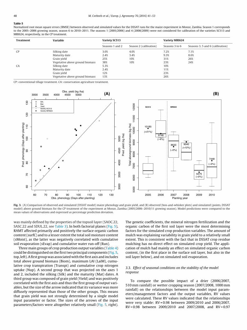

48 M. Corbeels et al. / Europ. J. Agronomy 76 (2016) 41–53

Table 5Normalized root mean square errors (RMSE) between observed and simulated values for the DSSAT runs for the maize experiment in Monze, Zambia. Season 1 correspondsto the 2005–2006 growing season, season 6 to 2010–2011. The seasons 1 (2005/2006) and 4 (2008/2009) were not considered for calibration of the varieties SC513 andMRI624, respectively, in the CP treatment.

Treatment Variable Variety SC513 Variety MRI624

Seasons 1 and 2 Season 2 (calibration) Seasons 3 to 6 Seasons 3, 5 and 6 (calibration)

CP Silking date 3.0% 4.0% 7.2% 7.1%Maturity date 2.4% 3.4% 9.3% 8.6%Grain yield 25% 10% 31% 26%Vegetative above ground biomass 38% 10% 23% 24%

CA Silking date 5.3% 10%Maturity date 2.4% 11%Grain yield 12% 23%Vegetative above ground biomass 13% 26%

CP: conventional tillage treatment. CA: conservation agriculture treatment.

(A) (B)

F and gm ambiam

wSRc(s

cttluatcadtip

ig. 3. (A) Comparison of observed and simulated (DSSAT model) maize phenologyodel) above ground biomass for the CP treatment of the experiment at Monze, Zean values of observations and expressed as percentage prediction deviation.

as mainly defined by the properties of the topsoil layer (SAOC.22,ASC.22 and SDUL.22, see Table 3). In both factorial planes (Fig. 5),AMT affected primarily and positively the surface organic carbonontent (surfC) and to a lesser extent the total soil moisture contentsMoist), as the latter was negatively correlated with cumulativeoil evaporation (sEvap) and cumulative water run-off (Run).

Three main groups of crop production output variables (Table 4)ould be distinguished on the first two principal components (Fig. 5,op, left). A first group was associated with the first axis and includesotal above ground biomass (Biom), maximum LAI (LaiM), cumu-ative crop transpiration (Transpi) and cumulative crop nitrogenptake (Nup). A second group that was projected on the axes 1nd 2, included the silking (Silk) and the maturity (Mat) dates. Ahird group was composed of grain yield (Yield) and was positivelyorrelated with the first axis and thus the first group of output vari-bles, but the size of the arrow indicated that its variance was more

iffusely represented than those of the other groups. This meanshat grain yield was not strongly determined by a single modelnput parameter or factor. The sizes of the arrows of the inputarameters/factors were altogether relatively small (Fig. 5, right).

rain yield, and (B) observed (box-and-whisker plots) and simulated (points, DSSAT (2005/2006–2010/11 growing season). Model predictions were compared to the

The genetic coefficients, the mineral nitrogen fertilization and theorganic carbon of the first soil layer were the most determiningfactors for the simulated crop production variables. The amount ofmulch was explaining variability in grain yield to a relatively smallextent. This is consistent with the fact that in DSSAT crop residuemulching has no direct effect on simulated crop yield. The appli-cation of mulch had mainly an effect on simulated organic carboncontent, (in the first place in the surface soil layer, but also in thesoil layer below), and on simulated soil evaporation.

3.3. Effect of seasonal conditions on the stability of the modelresponse

To compare the possible impact of a drier (2006/2007,510 mm rainfall) or wetter cropping season (2007/2008, 1000 mmrainfall) on the relationships between the model input param-

eters/management factors and the output variables, RV valueswere calculated. These RV values indicated that the relationshipswere very stable: RV = 0.98 between 2009/2010 and 2006/2007,RV = 0.98 between 2009/2010 and 2007/2008, and RV = 0.97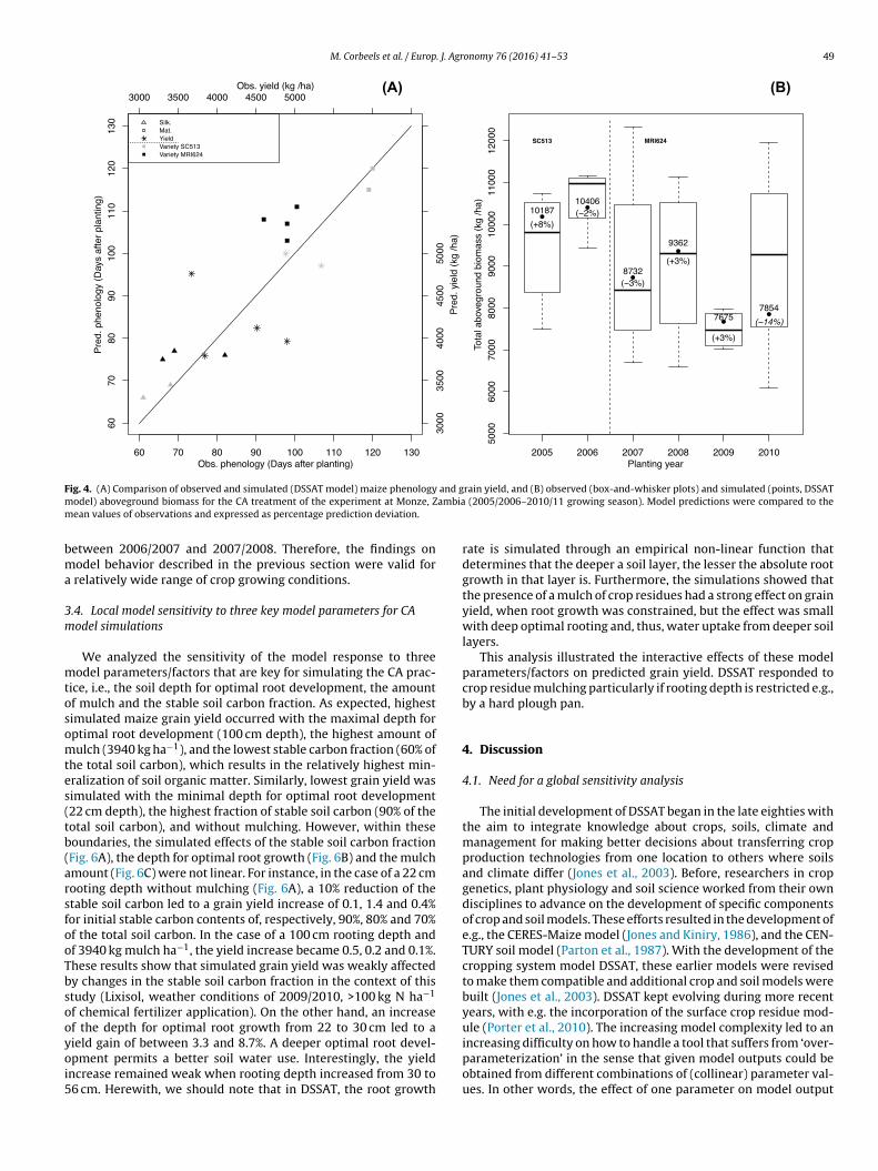

M. Corbeels et al. / Europ. J. Agronomy 76 (2016) 41–53 49

(A) (B)

F and gm ambiam

bma

3m

mtosomtes(tb(arsfooTbsooyoi5

ig. 4. (A) Comparison of observed and simulated (DSSAT model) maize phenologyodel) aboveground biomass for the CA treatment of the experiment at Monze, Zean values of observations and expressed as percentage prediction deviation.

etween 2006/2007 and 2007/2008. Therefore, the findings onodel behavior described in the previous section were valid for

relatively wide range of crop growing conditions.

.4. Local model sensitivity to three key model parameters for CAodel simulations

We analyzed the sensitivity of the model response to threeodel parameters/factors that are key for simulating the CA prac-

ice, i.e., the soil depth for optimal root development, the amountf mulch and the stable soil carbon fraction. As expected, highestimulated maize grain yield occurred with the maximal depth forptimal root development (100 cm depth), the highest amount ofulch (3940 kg ha−1), and the lowest stable carbon fraction (60% of

he total soil carbon), which results in the relatively highest min-ralization of soil organic matter. Similarly, lowest grain yield wasimulated with the minimal depth for optimal root development22 cm depth), the highest fraction of stable soil carbon (90% of theotal soil carbon), and without mulching. However, within theseoundaries, the simulated effects of the stable soil carbon fractionFig. 6A), the depth for optimal root growth (Fig. 6B) and the mulchmount (Fig. 6C) were not linear. For instance, in the case of a 22 cmooting depth without mulching (Fig. 6A), a 10% reduction of thetable soil carbon led to a grain yield increase of 0.1, 1.4 and 0.4%or initial stable carbon contents of, respectively, 90%, 80% and 70%f the total soil carbon. In the case of a 100 cm rooting depth andf 3940 kg mulch ha−1, the yield increase became 0.5, 0.2 and 0.1%.hese results show that simulated grain yield was weakly affectedy changes in the stable soil carbon fraction in the context of thistudy (Lixisol, weather conditions of 2009/2010, >100 kg N ha−1

f chemical fertilizer application). On the other hand, an increasef the depth for optimal root growth from 22 to 30 cm led to a

ield gain of between 3.3 and 8.7%. A deeper optimal root devel-pment permits a better soil water use. Interestingly, the yield

ncrease remained weak when rooting depth increased from 30 to6 cm. Herewith, we should note that in DSSAT, the root growth

rain yield, and (B) observed (box-and-whisker plots) and simulated (points, DSSAT (2005/2006–2010/11 growing season). Model predictions were compared to the

rate is simulated through an empirical non-linear function thatdetermines that the deeper a soil layer, the lesser the absolute rootgrowth in that layer is. Furthermore, the simulations showed thatthe presence of a mulch of crop residues had a strong effect on grainyield, when root growth was constrained, but the effect was smallwith deep optimal rooting and, thus, water uptake from deeper soillayers.

This analysis illustrated the interactive effects of these modelparameters/factors on predicted grain yield. DSSAT responded tocrop residue mulching particularly if rooting depth is restricted e.g.,by a hard plough pan.

4. Discussion

4.1. Need for a global sensitivity analysis

The initial development of DSSAT began in the late eighties withthe aim to integrate knowledge about crops, soils, climate andmanagement for making better decisions about transferring cropproduction technologies from one location to others where soilsand climate differ (Jones et al., 2003). Before, researchers in cropgenetics, plant physiology and soil science worked from their owndisciplines to advance on the development of specific componentsof crop and soil models. These efforts resulted in the development ofe.g., the CERES-Maize model (Jones and Kiniry, 1986), and the CEN-TURY soil model (Parton et al., 1987). With the development of thecropping system model DSSAT, these earlier models were revisedto make them compatible and additional crop and soil models werebuilt (Jones et al., 2003). DSSAT kept evolving during more recentyears, with e.g. the incorporation of the surface crop residue mod-ule (Porter et al., 2010). The increasing model complexity led to an

increasing difficulty on how to handle a tool that suffers from ‘over-parameterization’ in the sense that given model outputs could beobtained from different combinations of (collinear) parameter val-ues. In other words, the effect of one parameter on model output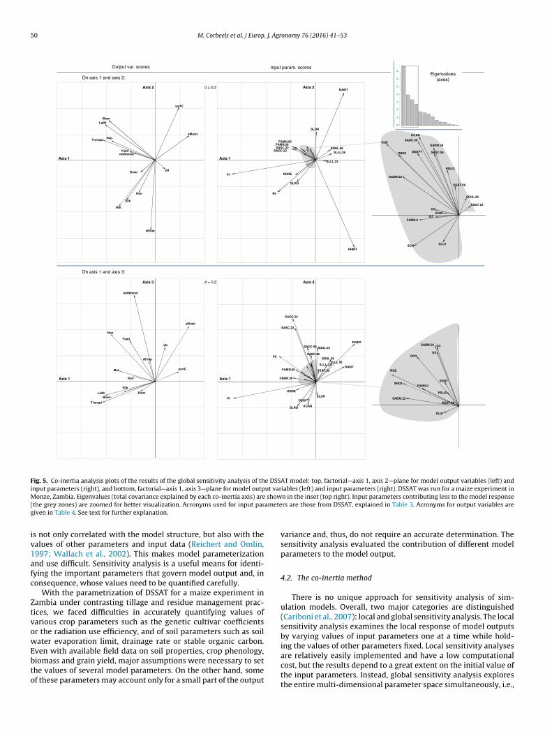

50 M. Corbeels et al. / Europ. J. Agronomy 76 (2016) 41–53

GDD EP1

P5

PHINT

SLDR

SLRO

SAOC.22

FAMN.30

RAMT

SASC.22

SLLL.22

SLLL.56SDUL.56

Axis 1

Axis 2

FAMN.50

d = 0.2

Eme r

Sil k

Mat

Yield

Biom

Transpi

sEvap

Nup

Run

LaiM

surfC

sMoist

sN

netNminer

RUE

KCAN

DSGFT

G2

G3

SLU1

SAD M.22

SH2O

SNO3

FAMN.0

PSLIG

SCN

SADM.56

SAOC.56

SASC.56

SDUL.22

SSAT.22

SSAT.56

0.0

0.5

1.0

1.5

2.0

2.5

3.0

3.5

Eigen value s(axes)

Output var. scores Inpu t pa ram. sc ores

On axis 1 and axis 2:

Axis 1

Axis 2

On axis 1 and axis 3:

d = 0.2

Eme r

Sil k

Mat

Yield

Biom

Transpi

sEvap

Nup

Run

LaiM

surfC

sMoist

sN

netNminer

KCAN

DSGFT

GDD E

P1

P5

PHINT

SLDR

SLRO

SAOC.22

FAMN.30

FAMN.50RAMT

SAOC.56

SASC.22

SASC.56

SLLL .22SLLL .56

SDU L.22

SSAT.22

SDU L.56

RUE

G2

G3

SLU1

SAD M.22

SH2OSNO3

FAMN.0

PSLIG

SCN

SAD M.56

SSAT.56

Axis 1

Axis 3

Axis 1

Axis 3

Fig. 5. Co-inertia analysis plots of the results of the global sensitivity analysis of the DSSAT model: top, factorial—axis 1, axis 2—plane for model output variables (left) andinput parameters (right), and bottom, factorial—axis 1, axis 3—plane for model output variables (left) and input parameters (right). DSSAT was run for a maize experiment inM show( ameteg

iv1afc

ZtvowEbto

onze, Zambia. Eigenvalues (total covariance explained by each co-inertia axis) arethe grey zones) are zoomed for better visualization. Acronyms used for input pariven in Table 4. See text for further explanation.

s not only correlated with the model structure, but also with thealues of other parameters and input data (Reichert and Omlin,997; Wallach et al., 2002). This makes model parameterizationnd use difficult. Sensitivity analysis is a useful means for identi-ying the important parameters that govern model output and, inonsequence, whose values need to be quantified carefully.

With the parametrization of DSSAT for a maize experiment inambia under contrasting tillage and residue management prac-ices, we faced difficulties in accurately quantifying values ofarious crop parameters such as the genetic cultivar coefficientsr the radiation use efficiency, and of soil parameters such as soilater evaporation limit, drainage rate or stable organic carbon.

ven with available field data on soil properties, crop phenology,iomass and grain yield, major assumptions were necessary to sethe values of several model parameters. On the other hand, somef these parameters may account only for a small part of the output

n in the inset (top right). Input parameters contributing less to the model responsers are those from DSSAT, explained in Table 3. Acronyms for output variables are

variance and, thus, do not require an accurate determination. Thesensitivity analysis evaluated the contribution of different modelparameters to the model output.

4.2. The co-inertia method

There is no unique approach for sensitivity analysis of sim-ulation models. Overall, two major categories are distinguished(Cariboni et al., 2007): local and global sensitivity analysis. The localsensitivity analysis examines the local response of model outputsby varying values of input parameters one at a time while hold-ing the values of other parameters fixed. Local sensitivity analyses

are relatively easily implemented and have a low computationalcost, but the results depend to a great extent on the initial value ofthe input parameters. Instead, global sensitivity analysis exploresthe entire multi-dimensional parameter space simultaneously, i.e.,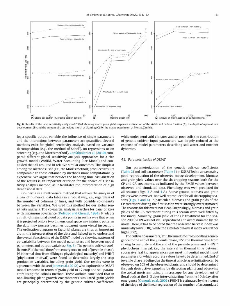

M. Corbeels et al. / Europ. J. Agronomy 76 (2016) 41–53 51

F d respd e expe

famdspgcaceotd

atbswaitTatcpfiP(pamena

ig. 6. Results of the local sensitivity analysis of DSSAT showing maize grain yielevelopment (B) and the amount of crop residue mulch at planting (C) for the maiz

or a specific output variable the influence of single parametersnd the interactions between parameters are quantified. Severalethods exist for global sensitivity analysis, based on variance

ecomposition (e.g., the method of Sobol’), on regressions or oncreening (e.g., the Morris method). Confalonieri et al. (2010) com-ared different global sensitivity analysis approaches for a ricerowth model (WARM, Water Accounting Rice Model) and con-luded that all resulted in relative similar outcomes. The simplestmong the methods used (i.e., the Morris method) produced resultsomparable to those obtained by methods more computationallyxpensive. We argue that besides the handling time, visualizationf the results is an important criterion for the choice of a sensi-ivity analysis method, as it facilitates the interpretation of highimensional data.

Co-inertia is a multivariate method that allows the analysis of pair of numerical data tables in a robust way, i.e., regardless ofhe number of columns or lines, and with possible co-linearityetween the variables. We used this method for our global sen-itivity analysis. The co-inertia analysis searches for pairs of axesith maximum covariance (Dolédec and Chessel, 1994). It adapts

multi-dimensional cloud of data points in such a way that whent is projected onto a two dimensional space any intrinsic patternshe data may possess becomes apparent upon visual inspection.he ordination diagrams or factorial planes are thus an importantid in the interpretation of the data and helped us to understandhe overall functioning of the DSSAT model by showing patterns ofo-variability between the model parameters and between modelarameters and output variables (Fig. 5). The genetic cultivar coef-cients P1 (thermal time from emergence to end of juvenile phase),5 (thermal time from silking to physiological maturity) and PHINTphyllocron interval) were found to determine largely the croproduction variables, including grain yield. Our results were ingreement with those of Jones et al. (2012) who explored the DSSATodel response in terms of grain yield to 17 crop and soil param-

ters using the Sobol’s method. These authors concluded that inon-limiting plant growth environments simulated grain yieldsre principally determined by the genetic cultivar coefficients,

onses as function of the stable soil carbon fraction (A), the depth of optimal rootriment at Monze, Zambia.

while under semi-arid climates and on poor soils the contributionof genetic cultivar input parameters was largely reduced at theexpense of model parameters describing soil water and nutrientdynamics.

4.3. Parameterisation of DSSAT

Our parameterization of the genetic cultivar coefficients(Table 2) and soil parameters (Table 1) in DSSAT led to a reasonablygood reproduction of the observed maize development, biomassand grain yield values over the six cropping seasons both for theCP and CA treatments, as indicated by the RMSE values betweenobserved and simulated data. Phenology was well predicted forall seasons (Figs. 3 A and 4 A). Above ground biomass and grainyields were, however, not well reproduced for all six cropping sea-sons (Figs. 3 and 4). In particular, biomass and grain yields of theCP treatment during the first season were strongly overestimated.The reasons for this were not clear. Surprisingly, biomass and grainyields of the CA treatment during this season were well fitted bythe model. Similarly, grain yield of the CP treatment for the sea-son 2008/2009 was not well reproduced and overestimated by themodel. Here, it has to be noted that the observed harvest index wasunusually low (0.38), while the simulated harvest index was ratherhigh (0.52).

The cultivar parameters, ‘P1′, thermal time from seedlings emer-gence to the end of the juvenile phase, ‘P5′, the thermal time fromsilking to maturity and the end of the juvenile phase and ‘PHINT’,phyllochron interval, i.e., the interval in thermal time betweensuccessive leaf tip appearances are most influential model inputparameters for which accurate values have to be determined. End ofjuvenile phase is defined as the time at which tassel initiation can beobserved on 50% of the observed plants, and should be determinedthrough destructive sampling by dissecting plants and observing

the apical meristem using a microscope for any development offloral buds at the 2–3 days interval starting from the 10th day afteremergence (Gungula et al., 2003). PHINT is estimated by the inverseof the slope of the linear regression of the number of accumulated

5 . J. Agr

otnptsaai

4

asnugrmist

cimwodMpc

owmen

5

esabpsClay(gtuutn

heCe

2 M. Corbeels et al. / Europ

r emerged leaves on the main stem against accumulated thermalime. Determining the number of fully expanded leaves and leaf tipseeds accurate (and weekly) monitoring of a sufficient number oflants under field conditions. For P5, time of silking is recorded inhe field when silks are noticed on 50% of the observed plants. In aimilar way, time of physiological maturity is recorded in the fields the day when 50% of the grains in each observed ear have formed

black layer, indicating that no further accumulation of assimilatess possible.

.4. DSSAT response to CA practice

The co-inertia analysis scores (Fig. 5) illustrated that the appliedmount of mulch (RAMT) strongly and positively affects simulatedoil surface carbon content (surfC) and soil moisture (sMoist), andegatively soil evaporation (sEvap) and runoff (Run). Consequently,nder drought stress the practice of mulching affects simulatedrain yield positively. Results from the local sensitivity analysis cor-oborated this. The application of a mulch of crop residues affected

ore positively simulated grain yield when water uptake was lim-ted as a result of limited optimal root growth, as compared to aituation with deep optimal root development and greater accesso more soil water.

To be able to reproduce with DSSAT the yield increase under CAompared to CP, it was necessary to include a rooting depth effect,n addition to the mulch and the no-tillage effects. Under CP opti-

al root development was restricted to the plough layer (22 cm),hile under CA roots could optimally develop to 100 cm depth. The

ccurrence of a hard pan caused by repeated ploughing to the sameepth is a common feature in loam and clay soils (Materechera andloza-Banda, 1997). A hard pan restricts root growth and water

ercolation, which can have severe effects on plant growth, espe-ially if the topsoil dries out (Adeoye and Mohamed-Saleem, 1990).

Finally, in our study, simulated effects of crop residue mulchingn soil carbon content and nitrogen immobilization/mineralizationere relatively small and had no effect on grain yield given theineral fertilizer application of 108 kg N ha−1 year−1. (Simulated)

ffects of the CA versus CP treatment on soil carbon become pro-ounced in the long term (Corbeels et al., 2014).

. Conclusions

The results of our study illustrate that in order to simulate yieldffects of CA, an agronomic diagnosis is required on what the site-pecific factors are that explain the yield differences between CAnd CP. Some of these factors are not mechanistically simulatedy DSSAT, but can be incorporated in the model through a properarameterisation of relevant parameters. This is the case for e.g.,oil structure differences as a result of the practice of CA versusP, which may have an effect on crop yield. DSSAT does not simu-

ate these soil structural effects. In our study we had to introduce rooting depth effect in order to reproduce the observed maizeield differences between the CP (tillage and no residues) and CAno-tillage and crop residue mulching). Under CP the optimal rootrowth was restricted to the upper 22 cm soil layer as a result ofhe formation of a hard pan just below ploughing depth, whilstnder CA optimal root growth in the model was unrestricted. Sim-lated effects of mulching on yields were more pronounced whenhe depth for optimal root development, and thus crop water (andutrient) uptake was restricted.

Co-inertia analysis was used in order to analyze and visualize

ow 16 DSSAT model output variables respond to 32 input param-ters, considering parameter correlations and nonlinear relations.o-inertia analysis can be used to visually inspect and identify influ-ntial model parameters that must be estimated from experiments

onomy 76 (2016) 41–53

and observations. On the other hand, those parameters with a smallcontribution to model output can be excluded from the calibrationexercise and can be set equal to any value within their range. Thiscontributes to a simplification of model use and is useful for calibra-tion of this type of complex crop growth models for multiple sitesor at a regional scale. Under the conditions of our study, geneticcultivar coefficients were the most influential model parameters.

Acknowledgments

This study has been carried out as part of the CA2AfricaCSA-SA project (no. 245347), EU 7th Framework Programme: ‘Con-servation Agriculture in AFRICA: Analyzing and FoReseeing itsImpact—Comprehending its Adoption’. The authors are grateful tothe colleagues of the AIDA research unit (CIRAD) for the discussionson the use of cropping systems models.

References

Adeoye, K.B., Mohamed-Saleem, M.A., 1990. Comparison of effects of some tillagemethods on soil physical properties and yield of maize and stylo in a degradedferruginous tropical soil. Soil Tillage Res. 18, 63–72.

Andales, A.A., Batchelor, W.D., Anderson, C.E., Farnham, D.E., Whigham, D.K., 2000.Incorporating tillage effects into a soybean model. Agric. Syst. 66, 69–98.

Blanco-Canqui, H., Lal, R., 2007. Soil structure and organic carbon relationshipsfollowing 10 years of wheat straw management in no-till. Soil Tillage Res. 95,240–254.

Cariboni, J., Gatelli, D., Liska, R., Saltelli, A., 2007. The role of sensitivity analysis inecological modelling. Ecol. Mode 203, 167–182.

Caviglia, O.P., Sadras, V.O., Andrade, F.H., 2013. Modelling long-term effects ofcropping intensification reveals increased water and radiation productivity inthe South-eastern Pampas. Field Crops Res. 149, 300–311.

Chessel, D., Mercier, P., 1993. Couplage de triplets statistiques et liaisonsespèces-environnement. In: Lebreton, J.D., Asselain, B. (Eds.), Biométrie etEnvironnement. Masson, Paris (France), pp. 15–44 (French).

Confalonieri, R., Bellocchi, G., Bregaglio, S., Donatelli, M., Acutis, M., 2010.Comparison of sensitivity analysis techniques: a case study with the ricemodel WARM. Ecol. Model. 221, 1897–1906.

Corbeels, M., De Graaff, J., Ndah, H.T., Penot, E., Baudron, F., Naudin, K., Andrieu, N.,Chirat, G., Schuler, J., Nyagumbo, I., Rusinamhodzi, L., Traore, K., Mzoba, H.D.,Adolwa, I.S., 2014. Understanding the impact and adoption of conservationagriculture in Africa: a multi-scale analysis. Agric. Ecosyst. Environ. 187,155–170.

Dolédec, S., Chessel, D., 1994. Co-inertia analysis: an alternative method forstudying species-environment relationships. Freshw. Biol. 31, 277–294.

Fofana, B., Tamélokpo, A., Wopereis, M.C.S., Breman, H., Dzotsi, K., Carsky, R.J.,2005. Nitrogen use efficiency by maize as affected by a mucuna short fallowand P application in the coastal savanna of West Africa. Nutr. Cycl. Agroecosyst.71, 227–237.

Gerardeaux, E., Giner, M., Ramanantsoanirina, A., Dusserre, J., 2011. Positive effectsof climate change on rice in Madagascar. Agron. Sustain. Dev., 1–9.

Gijsman, A.J., Hoogenboom, G., Parton, W.J., Kerridge, P.C., 2002. Modifying DSSATcrop models for low-input agricultural systems using a soil organicmatter-residue module from CENTURY. Agron. J. 94, 462–474.

Giller, K.E., Witter, E., Corbeels, M., Tittonell, P., 2009. Conservation agriculture andsmallholder farming in Africa: the heretics’ view. Field Crops Res. 114, 23–34.

Gowing, J.W., Palmer, M., 2008. Sustainable agricultural development insub-Saharan Africa: the case for paradigm shift in land husbandry. Soil UseManage. 24, 92–99.

Gungula, D.T., Kling, J.G., Togun, A.O., 2003. CERES-maize predictions of maizephenology under nitrogen-stressed conditions in Nigeria. Agron. J. 95,892–899.

He, J., Jones, J.W., Graham, W.D., Dukes, M.D., 2010. Influence of likelihood functionchoice for estimating crop model parameters using the generalized likelihooduncertainty estimation method. Agric. Syst. 103, 256–264.

Jagtap, S.S., Abamu, F.J., 2003. Matching improved maize production technologiesto the resource base of farmers in a moist savanna. Agric. Syst. 76, 1067–1084.

Jones, J.W., Hoogenboom, G., Porter, C.H., Boote, K.J., Batchelor, W.D., Hunt, L.A.,Wilkens, P.W., Singh, U., Gijsman, A.J., Ritchie, J.T., 2003. The DSSAT croppingsystem model. Eur. J. Agron. 18, 235–265.

Jones, J.W., Kiniry, J.R. (Eds.), 1986. CERES-maize, a simulation model of maizegrowth and development. T&M University Press, College Station.

Jones, J.W., Naab, J., Fatondji, D., Dzotsi, K.A., Adiku, S., He, J., 2012. Uncertainties insimulating crop performance in degraded soils and low input productionsystems. In: Kihara, J., Fatondji, D., Jones, J.W., Hoogenboom, G., Tabo, R.,

Bationo, A. (Eds.), Improving Soil Fertility Recommendations in Africa UsingDecision Support for Agro-technology Transfers (DSSAT). Springer, pp. 43–59.

Keating, B.A., Carberry, P.S., Hammer, G.L., Probert, M.E., Robertson, M.J.,Holzworth, D., Huth, N.I., Hargreaves, J.N.G., Meinke, H., Hochman, Z., McLean,G., Verburg, K., Snow, V., Dimes, J.P., Silburn, M., Wang, E., Brown, S., Bristow,

. J. Agr

L

M

M

M

N

O

P

P

P

R

R

R

R

R

Integrated Approaches to Higher Maize Productivity in the New Millennium.CIMMYT, Kenya Agricultural Research Institute, Nairobi (Kenya), pp. 338–342.

Wallach, D., Goffinet, B., Tremblay, M., 2002. Parameter estimation in crop models:

M. Corbeels et al. / Europ

K.L., Asseng, S., Chapman, S., McCown, R.L., Freebairn, D.M., Smith, C.J., 2003.An overview of APSIM, a model designed for farming systems simulation. Eur.J. Agron. 18, 267–288.

indquist, J.L., Arkebauer, T.J., Walters, D.T., Cassman, K.G., Dobermann, A., 2005.Maize radiation use efficiency under optimal growth conditions. Agron. J. 97,72–78.

acCarthy, D.S., Vlek, P.L.G., Bationo, A., Tabo, R., Fosu, M., 2010. Modeling nutrientand water productivity of sorghum in smallholder farming systems in asemi-arid region of Ghana. Field Crops Res. 118, 251–258.

aterechera, S.A., Mloza-Banda, H.R., 1997. Soil penetration resistance, rootgrowth and yield of maize as influenced by tillage system on ridges in Malawi.Soil Tillage Res. 41, 13–24.

cKay, M.D., Conover, W.J., Beckman, R.J., 1979. A comparison of three methodsfor selecting values of input variables in the analysis of output from acomputer code. Technometrics 21, 239–245.

gwira, A.R., Aune, J.B., Thierfelder, C., 2014. DSSAT modelling of conservationagriculture maize response to climate change in Malawi. Soil Tillage Res. 143,85–94.

gindo, H.O., Walker, S., 2005. Comparison of measured changes in seasonal soilwater content by rainfed maize-bean intercrop and component croppingsystems in a semi-arid region of southern Africa. Phys. Chem. Earth 30,799–808.

arton, W.J., Schimel, D.S., Cole, C.V., Ojima, D.S., 1987. Analysis of factorscontrolling soil organic matter levels in Great Plains grasslands. Soil Sci. Soc.Am. J. 51, 1173–1179.

athak, T.B., Fraisse, C.W., Jones, J.W., Messina, C.D., Hoogenboom, G., 2007. Use ofglobal sensitivity analysis for CropGro cotton model development. Am. Soc.Agric. Biol. Eng. 50, 2295–2302.

orter, C., Jones, J., Adiku, S., Gijsman, A., Gargiulo, O., Naab, J., 2010. Modelingorganic carbon and carbon-mediated soil processes in DSSAT v4.5. Oper. Res.10, 247–278.

Development Core Team, 2009. R: A Language and Environment for StatisticalComputing. R Foundation for Statistical Computing, Vienna, Austria.

eichert, P., Omlin, M., 1997. On the usefulness of over-parameterized ecologicalmodels. Ecol. Model. 95, 289–299.

itchie, J.T., 1998. Soil water balance and plant water stress. In: Tsuji, G.Y., et al.(Eds.), Understanding Options of Agricultural Production, Kluwer AcademicPubl. and Int. Consortium for Agriciltural Systems Applications, Dordrecht, TheNetherlands, pp. 41–53.

itchie, J.T., Porter, C.H., Judge, J., Jones, J.W., Suleiman, A.A., 2009. Extension of anexisting model for soil water evaporation and redistribution under high watercontent conditions. Soil Sci. Soc. Am. J. 73, 792–801.

obert, P., Escoufier, Y., 1976. A unifying tool for linear multivariate statisticalmethods: the RV-coefficient. Appl. Stat. 25, 257–265.

onomy 76 (2016) 41–53 53

Rusinamhodzi, L., Corbeels, M., van Wijk, M.T., Rufino, M.C., Nyamangara, J., Giller,K.E., 2011. A meta-analysis of long-term effects of conservation agriculture onmaize yields under rain-fed conditions: lessons for southern Africa. Agron.Sustain. Dev. 31, 657–673.

Saseendran, S.A., Ma, L., Malone, R., Heilman, P., Ahuja, L.R., Kanwar, R.S., Karlen,D.L., Hoogenboom, G., 2007. Simulating management effects on cropproduction, tile drainage, and water quality using RZWQM-DSSAT. Geoderma140, 297–309.

Scopel, E., da Silva, F.A.M., Corbeels, M., Affholder, F., Maraux, F., 2004. Modellingcrop residue mulching effects on water use and production of maize undersemi-arid and humid tropical conditions. Agronomie 24, 1–13.

Six, J., Conant, R.T., Paul, E.A., Paustian, K., 2002. Stabilization mechanisms of soilorganic matter: implications for C-saturation of soils. Plant Soil 241, 155–176.

Sommer, R., Wall, P.C., Govaerts, B., 2007. Model-based assessment of maizecropping under conventional and conservation agriculture in highland Mexico.Soil Tillage Res. 94, 83–100.

Thierfelder, C., Mwila, M., Rusinamhodzi, L., 2013. Conservation agriculture ineastern and southern provinces of Zambia: long-term effects on soil qualityand maize productivity. Soil Tillage Res. 126, 246–258.

Thierfelder, C., Wall, P.C., 2009. Effects of conservation agriculture techniques oninfiltration and soil water content in Zambia and Zimbabwe. Soil Tillage Res.105, 217–227.

Thierfelder, C., Wall, P.C., 2010. Investigating conservation agriculture (ca) systemsin Zambia and Zimbabwe to mitigate future effects of climate change. J. CropImprov. 24, 113–121.

Thierfelder, C., Rusinamhodzi, L., Ngwira, A.R., Mupangwa, W., Nyagumbo, I.,Kassie, G.T., Cairns, J.E., 2014. Conservation agriculture in Southern Africa:advances in knowledge. Renew. Agric. Food Syst. 30, 328–348.

Thioulouse, J., Lobry, J.R., 1995. Co-inertia analysis of amino-acid physico-chemicalproperties and protein composition with the ADE package. Comp. Appl. Biosci.:CABIOS 11, 321–329.

Uri, N.D., 2000. An evaluation of the economic benefits and costs of conservationtillage. Environ. Geol. 39, 238–248.

Waddington, S.R., Karigwindi, J., 2004. Longer-term contribution of groundnutrotation and cattle manure to the sustainability of maize-legume smallholdersystems in sub-humid Zimbabwe. In: Friesen, D.K., Palmer, A.F.E. (Eds.),

exploring the possibility of estimating linear combinations of parameters.Agronomie 22, 171–178.