event-triggered natural hazard monitoring with ... · hazard with respect to process understanding...
TRANSCRIPT

Event-triggered Natural Hazard Monitoringwith Convolutional Neural Networks on the Edge
Matthias MeyerComputer Engineering and Networks
Laboratory, ETH ZurichZurich, Switzerland
Timo Farei-CampagnaComputer Engineering and Networks
Laboratory, ETH ZurichZurich, Switzerland
Akos PasztorComputer Engineering and Networks
Laboratory, ETH ZurichZurich, Switzerland
Reto Da FornoComputer Engineering and Networks
Laboratory, ETH ZurichZurich, Switzerland
Tonio GsellComputer Engineering and Networks
Laboratory, ETH ZurichZurich, Switzerland
Samuel WeberComputer Engineering and Networks
Laboratory, ETH ZurichZurich, Switzerland
Jan BeutelComputer Engineering and Networks
Laboratory, ETH ZurichZurich, Switzerland
Lothar ThieleComputer Engineering and Networks
Laboratory, ETH ZurichZurich, Switzerland
ABSTRACTIn natural hazard warning systems fast decision making is vitalto avoid catastrophes. Decision making at the edge of a wirelesssensor network promises fast response times but is limited by theavailability of energy, data transfer speed, processing and memoryconstraints. In this workwe present a realization of awireless sensornetwork for hazard monitoring which is based on an array of event-triggered seismic sensors with advanced signal processing andcharacterization capabilities for a novel co-detection technique. Onthe one hand we leverage an ultra-low power, threshold-triggeringcircuit paired with on-demand digital signal acquisition capableof extracting relevant information exactly when it matters mostand not wasting precious resources when nothing can be observed.On the other hand we use machine-learning-based classificationimplemented on low-power, off-the-shelf microcontrollers to avoidfalse positive warnings and to actively identify humans in hazardzones. The sensors’ response time and memory requirement is sub-stantially improved by pipelining the inference of a convolutionalneural network. In this way, convolutional neural networks thatwould not run unmodified on a memory constrained device can beexecuted in real-time and at scale on low-power embedded devices.
KEYWORDSNatural Hazard Warning System, Wireless Sensing Platform, Con-volutional Neural Network, Machine Learning, On-device Classifi-cation
1 INTRODUCTIONIn the following we present a scenario where it is mandatory toperform complex decision making on the edge of a distributedinformation processing system and show based on a case-studyhow the approach can be embedded into a wireless sensor networkarchitecture.
Natural disasters happen infrequently and for mitigation effortsfast reaction times relative to these rarely occurring events is im-portant, especially critical infrastructure or even human casualtiesare at stake [14]. In alpine regions where human habitats includingsettlements and infrastructure are threatened by rockfalls, wirelesssensor networks can act as a natural warning systems [17]. Theyhave the flexibility to be deployed in locations that are logisticallydifficult or dangerous to access, for example an active rockfall scarp.Therefore it is important that these systems run autonomously forlong periods of time [13].
Traditionally, continuous, high-resolution data acquisition isused to monitor micro-seismic signals emanating from structuralfatigue [2, 23]. These methods are powerful in capturing naturalhazard with respect to process understanding as well as hazardwarning. However, they suffer severely that in periods of no or lit-tle activity continuous high-rate signal amplification and samplingdoes not provide an information gain while consuming energy. Inaddition, they scale unfavorably due to the large amount of dataproduced [38]. A novel approach, based on a coupled fibre-bundlemodel, exists that registers precursory patterns of catastrophicevents with the help of many threshold triggered sensors and areduced set of explanatory variables. Furthermore increasing thenumber of sensor nodes leads to a largely improved detection capa-bility limited only by the available transmission bandwidth if datais to be processed centrally. One way to reduce the network utiliza-tion is to make the sensors themselves more intelligent by shiftingthe knowledge generation process from the centralized backendcloser to the signal sources. Thus, a system that is optimized tocalculate explanatory variables directly on the sensor can reducethe logging and transmission cost and also allowing to react withhigh reactivity on the detection of catastrophic events.
But such an extreme reduction in information content comesat a price: false positives and the inability to characterize events
arX
iv:1
810.
0940
9v1
[cs
.LG
] 2
2 O
ct 2
018

M. Meyer et al.
further. While the first has an impact on correct analysis and net-work metrics, the latter is of importance to react adequately on thedetection of a disaster. For example if humans are present in a haz-ard zone they should be warned and a search and rescue missionshould be dispatched immediately. Correct and timely informa-tion here is of utmost importance to maximize success and avoidexpensive interventions on false alarms. Under the constraintsgiven, on-device classification provides a mean to identify humanson-location without the requirement to transmit all sensory datathrough the network.
We present a system architecture for natural hazard monitoringusing seismic sensors (geophones) that can be used for detection ofprecursory rockfall patterns based on the theory of co-detection.Furthermore we present a concept for accurate on-sensor classi-fication of seismic signals to reduce false positives and enhanceinformation by identifying humans in the signal using machinelearning techniques.
We evaluate our network and system architecture in two scenar-ios. In the first scenario we present an outdoor, wide-area sensingsystem presently located at two locations in high alpine environ-ments. We demonstrate the functionality of our system architectureand evaluate the suitability for rockfall detection using co-detectionof seismic events. The second scenario is a laboratory experimentto demonstrate the feasibility of on-device classification using con-volutional neural networks within the wireless sensor architecture.We focus on advanced methods to reduce the memory requirementsand latency of an embedded convolutional neural network classifier.
In this context the paper contains the following contributions
• A realization of a wireless, event-triggered, micro-seismicsensor system featuring low-power consumption, fast wake-up time and on-device signal characterization. The system isrealized using open source hardware and protocol designs.
• An implementation of a convolutional neural network forseismic event classification on low-power embedded devicesusing structural optimization and network quantization.
• A sophisticated buffering concept for pipelined inference of aconvolutional neural network to relax memory requirementsand to decrease latency.
2 RELATEDWORKRockfall Detection using Seismic Sensors: Seismic precursorypatterns before rockfalls have been investigated for several fieldsites [2, 28, 29]. These studies are based on micro-seismic mea-surements with a portable data logger. Wireless sensor networkshave been introduced to cover a larger area while removing therequirement of data retrieval [11, 23, 37]. They either provide theoption for remote data download or transmit short, event-triggeredsegments. Unlike in our study, event triggering is done in the digitaldomain which means that the acquisition system is constantly on.
Acoustic Event Detection: Artificial neural networks havebeen applied to acoustic event classification [6, 7, 16, 35] whichincludes among others footstep detection. Also footstep detectionand person identification using geophones has been studied before[3, 25], however only in experiments in a controlled environment.Artificial neural networks have been recently applied to seismic
Big EventCo-detection
Small Event Rockfall Detection
Footstep Detection
Post Analysis
Figure 1: Conceptual illustration of a wireless sensor net-work for natural hazard monitoring and the principle ofco-detection. Multiple seismic sensors are deployed in ahazardous area. The sensors feature the same hardware, aseismic sensor (geophone), processing, storage and wirelesscommunication subsystems, that are able to detect and clas-sify e.g. rockfall or footsteps. If a sensor detects an eventit can determine if it originates from a human in the haz-ard zone or not and possibly trigger an alert. If not it onlysends the event information trough a wireless low-powernetwork. A basestation collects the information from allsensors for centralized data gathering and further analysisusing post-processing methods. Temporal correlation of de-tected events, e.g. when multiple sensors register an eventwithin the same time window, it is possible to identify largemass failures or their precursors using the theory of co-detection [12].
event detection [24]. Especially convolutional neural networks haveachieved good accuracies [22, 26].
Artificial Neural Networks on Embedded Devices: Manystudies focus on additional accelerators [4, 8, 15] for convolutionalneural networks. This approach requires dedicated hardware. Stud-ies on mobile platforms [39] and wearables [18] exist but requirea more powerful hardware architecture. A prominent work forlow-power embedded devices focuses on keyword spotting [40]on a slightly more powerful Cortex-M7 than used in our study. Atheoretic strategy for low-memory convolutional neural networksas been proposed in [5] which focuses on an incremental depth-firstprocessing idea that resembles our approach. However, they neitherfocus on sequential data nor on the implementation with a specificbuffering system.
3 SYSTEM DESIGNFigure 1 illustrates the overall system design. A wireless sensornetwork consisting of multiple seismic nodes is deployed in anarea where rockfall occurs. The system can be partitioned intosensor nodes that are only used as rockfall detectors (light blue)and sensor nodes that additionally can classify footsteps (dark blue).The two node types have different requirements which will bebriefly outlined in the following.

Event-triggered Natural Hazard Monitoringwith Convolutional Neural Networks on the Edge
3.1 Rockfall Detection by Co-detection ofSeismic Events
The following describes the principle of detecting precursors ofrockfall patterns [12] with threshold triggered geophone sensors.Multiple geophones are deployed on the rock surface as illustratedin Figure 1. If rockfall stimulates a seismic event either due to frac-turing/detaching or due to impact, different sensors may register asignal depending on their location relative to the event source. Ahigh amplitude input signal registered at a single sensor can havetwo causes: Either a large event occurred at distance or a small eventoccurred in close proximity to the sensor. A co-detection exists ifmultiple sensors register an event quasi-simultaneously, which al-lows to distinguish between the two aforementioned possibilities.Furthermore, as lab experiments have shown [12], consecutive co-detections of events can be used to identify rockfall precursors andthus facilitates natural hazard earlywarning capabilities. Fundamen-tal for this principle is the requirement of many sensors to performco-detection as well as to cover a large enough area. The data acqui-sition can be reduced to only capture events, recording the exacttimestamp when the signal exceeds a certain threshold. While thisdetection can be implemented very efficiently in hardware using ananalog comparator circuit further analysis using signal processingtechniques require a digitizer and processing unit, typically putto sleep when not in use. A predictable system behaviour and aprecise time synchronization between all system components andall nodes is important to quantify co-detected events. A similar sys-tem based on much higher frequency acoustic emission signals hasbeen implemented successfully using the Dual Processor Platformarchitecture [34] and the event-based Low-PowerWireless Bus [33].We adopt these openly available system components to realize anoutdoor, wide-area sensing system, evaluate and demonstrate itsapplicability to perform co-detection of precursory rockfall patternsbased on low-frequency seismic signals.
3.2 Event Classification with Time DistributedProcessing
The co-detection concept allows to reduce false positives, e.g. byanthropogenic activity like humans walking by. However, to iden-tify whether a human is present on-site is impossible by just usingthe reduced set of information transmitted by the event-triggeredsensors, i.e. the timestamps of detected events. Since transmittingthe raw sensor data of each detected event in real-time for manysensor is infeasible due to bandwidth and energy limitations anapproach using on-device classification is advocated but severalchallenges need to be addressed. Multiple footstep detectors usinggeophones have been proposed [3, 25] but have not been shown todistinguish well between footsteps and seismic events [22]. Convo-lutional neural networks have shown to be good signal processingtools for classification of acoustic [16] as well as seismic sources[26]. However, convolutional neural networks have a high memorydemand, high memory access rates and a high processing demand.Typical commercially available low-power embedded devices areequipped with two types of memories, static random-access mem-ory (SRAM) and flash memory. On low-power devices the impact ofmemory usage on the energy efficiency is significant and space inenergy-efficient memory (SRAM) is limited. However, the inference
2018-09-06T06:48:07 CEST 2018-09-06T06:52:07 CEST
04:00Sep 6, 2018
06:00 08:00 10:00 12:00
1
2
3
4
5
Date
Num
ber
of C
o-de
tect
ions
Figure 2: An example of a rockfall event during the test-ing phase of the wireless sensor network. Illustrated is datafrom the monitoring system and two images (before andafter significant rockfall) taken with a remotely controlledhigh-resolution camera. The top plot shows how a clusterof sensors (see Figure 8) co-detected an event over time.The point size indicates the maximum peak amplitude de-tected in each co-detection within a 0.5 second time windowwhereas the vertical axis denotes how many sensors trig-geredwithin this window.Marked in pink on the right-handimage are the areas of rockmovementwhichwere identifiedby comparing the two images. The mountaineer visible inthe lower left corner of the left image is in the danger zonewith a number of significant impacts visible in its immedi-ate vicinity (pink). Locals reported that no one was harmedin this incident.
of a convolutional neural network requires a significant amount ofmemory to perform the computations, especially for storing inter-mediate results and the network parameters. Non-volatile memory,such as flash memory, is typically used to store the parameters ofthe neural network but the number of read accesses to this typeof memory should be minimized since the energy consumption istypically about 6x as high as reading from SRAM [36]. As a con-sequence it is important to reduce the memory requirement forthe parameters, for example by binarization of the network [19].However this approach comes with a drop in accuracy of about10%. In our work we apply incremental network quantization [41],which does not suffer from a reduced accuracy while reducing thenetwork parameter’s memory requirement.

M. Meyer et al.
For storing intermediate results SRAM is themost energy-efficientmemory. However, the intermediate results of state-of-the-art con-volutional neural networks do not fit into SRAM. Additionally, con-volutional neural networks suffer from a high latency because ofthe high number of operations required to perform a classification.
In this work we present a novel method to pipeline the compu-tations which relaxes the memory requirements significantly andallows to compute a convolutional neural network in SRAM onlywhile providing a low latency. In the following we call this concepttime distributed processing.
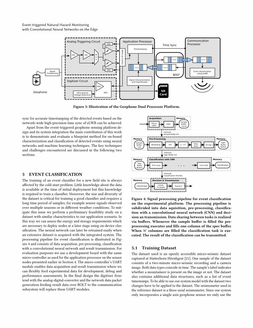
4 WIRELESS SENSING PLATFORMThe wireless seismic sensing platform presented in this paper isdepicted in Figure 3 and consists of the geophone sensor, an analogtriggering circuit, a digitizer circuit, an application processor, acommunication processors and a state-full processor interconnect.The geophone signal is conditioned and fed to the analog triggeringcircuit and digitizer circuit. The analog triggering circuit providesthe application processor with an interrupt signal if the geophonesignal is higher or lower than a given threshold. The applicationprocessor will timestamp the detected event and then enable thedigitizer system to sample the geophone signal for a pre-definedduration. The processing system is based on the Dual ProcessorPlatform (DPP) partitioning and decoupling the sensing applicationand the communication onto dedicated processing resources. Theinterconnect on DPP is realized using BOLT, an ultra-low powerprocessor state-full interconnect which features bi-directional, asyn-chronous message transfer and predictable run-time behaviour. Thecommunication subsystem is based on an IEEE 802.15.4-compatibletransceiver (MSP CC430) using eLWB [33].
4.1 Analog Triggering SubsystemThe circuit must be capable of amplifying the geophone sensor(SM-6 14Hz Omni-tilt Geophone, ION Geophysical Corporation)signal and comparing it to a predefined threshold trigger. Thispart of the system is always active, therefore it is most sensitivewith regards to power consumption since all other system com-ponents can be duty-cycled but the trigger must remain poweredat all times. An evaluation of different implementation variantsshowed the superiority of a fully discrete external solution (140.5,115.2, 22.9 uA respectively) among variants using OPAMP, DACand comparator circuits internal to the application processor (32-bitARM-Cortex-M4, STM32L496VG, 80MHz core clock, 3 uA currentdrain in STOP 2 mode with full RAM retention with RTC on; 1MBflash, 320 kB continuous SRAM), a mix with external and internalcomponents or all-external components. The final design incor-porates a dual-sided trigger with individual threshold set-pointsand a variable amplification (20x and 200x) using MAX5532 12-bitDACs and MAX9019 comparators. The input signal is biased tohalf the rail voltage and the upper and lower thresholds can beselected between 0 − Vsys/2 and Vsys/2 − Vsys respectively. Al-though (in theory) one single-sided trigger should be sufficient, wedeliberately chose to implement a dual-trigger system (triggeringboth on a rising and falling first edge of the seismic signal) to beable to have more degrees of freedom and stronger control overthe trigger settings chosen. The overhead for the bipolar trigger
system relative to the whole systems power figures in it’s differentoperating modes is negligible (see Section 7).
4.2 Digitizer SubsystemUpon detection of a threshold crossing of the incoming sensorsignal the application processor is woken up from an external in-terrupt and a timestamp of this event is stored. Subsequently thedata acquisition system, a 24-bit delta-sigma ADC with high SNRand built-in Programmable Gain Amplifier and low noise, high-precision voltage reference (MAX11214 ADC) is powered on andinitialized. It samples the geophone signal at 1 ksps and stores datain SD card storage until the signal remains below the trigger thresh-old values for a preconfigured duration (post-trigger interval). Forthis purpose all successive threshold crossings of the sensor signal(the interrupts) are monitored. After ADC sampling has completedthe ADC is switched off and all data describing the detected event(event timestamp, pos/neg threshold trigger counts, event duration,peak amplitude, position of peak amplitude) are assembled intoa data packet that is queued for transmission over the wirelessnetwork along with further health and debug data packets. Usingthis data, rockfall detection by means of co-detection as describedearlier in section 3.1 can commence using only very lightweightdata traffic while the full waveform data is available for furtherprocessing and event classification as presented later in section 5.
4.3 Wireless Communication SystemThe communication system is based on the TI CC430 system-on-chip running an adapted version of the event-based Low-PowerWireless Bus (eLWB) [33] based on Glossy. This protocol provideslow-latency and energy-efficiency for event-triggered data dissemi-nation using interference-based flooding. Since the protocol wasspecifically designed to be triggered by ultra-low power wake-upcircuits it is optimally suited for our application. We use the openlyavailable code1 with adaptations specific to our platform and thedata to be transferred.
4.4 Application IntegrationThe Dual Processor Platform (DPP) philosophy using the BOLTstate-full processor interconnect builds on the paradigm of sep-aration of concerns, shielding different system components andrun-time functionality from each other for as much as possible. Asa side effect this partitioning allows for easy integration and adap-tion to new applications and/or specifications by allowing to workon communication and application separately. Also, by using well-defined and strongly de-coupled interfaces application re-use isfacilitated. In BOLT two queues implemented on non-volatile mem-ory form a strictly asynchronous interface between two processorswith guaranteed maximum access times. The obvious drawback ofthis strict de-coupling however is, that all interaction between thetwo processors is message based and incurs different end-to-enddelays depending on queue fill and access patterns. Therefore tighttime synchronization is not readily available. For this purpose adedicated sync signal is routed between interrupt capable IOs of thetwo processors. In this way both the decoupling of the two applica-tion contexts for sensing and communication as well as tight time1https://github.com/ETHZ-TEC/LWB
Event-triggered Natural Hazard Monitoringwith Convolutional Neural Networks on the Edge
∙∙∙
Analog Triggering Circuit
∙∙∙
20x 10x MUX
∙∙∙
∙∙∙
BOLT
+
_
+
_
DAC
DAC
Digitizer Circuit
Geophone
SignalConditioning
Ultra-preciseVoltage Reference
PGA
ADC
CommunicationProcessor
Application Processor
SDCard
Signal Characterizationand Classification
Wake
-up
Contro
l
Event dissiminationusing eLWB
Time SyncTimestamping
Figure 3: Illustration of the Geophone Dual Processor Platform.
sync for accurate timestamping of the detected events based on thenetwork-wide high-precision time sync of eLWB can be achieved.
Apart from the event-triggered geophone sensing platform de-sign and its system integration the main contribution of this workis to demonstrate and evaluate a blueprint method for on-boardcharacterization and classification of detected events using neuralnetworks and machine learning techniques. The key techniquesand challenges encountered are discussed in the following twosections.
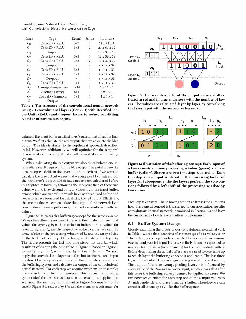
5 EVENT CLASSIFICATIONThe training of an event classifier for a new field site is alwaysaffected by the cold-start problem: Little knowledge about the datais available at the time of initial deployment but this knowledgeis required to train a classifier. Moreover, the size and diversity ofthe dataset is critical for training a good classifier and requires along time period of samples, for example sensor signals observedover multiple seasons or in different weather conditions. To mit-igate this issue we perform a preliminary feasibility study on adataset with similar characteristics to our application scenario. Inthis way we can assess the energy and storage requirements whichare necessary to deploy nodes at a later stage using on-device clas-sification. The neural network can later be retrained easily whenan extensive dataset is acquired with the integrated system. Theprocessing pipeline for event classification is illustrated in Fig-ure 4 and consists of data acquisition, pre-processing, classificationwith a convolutional neural network and result transmission. Forevaluation purposes we use a development board with the samemicro-controller as used for the application processor on the sensornodes presented earlier in Section 4. The micro-controller’s UARTmodule enables data acquisition and result transmission where wecan flexibly feed experimental data for development, debug andperformance assessments. In the final design the digitizer fron-tend with the analog-digital-converter and the network data packetgeneration feeding result data over BOLT to the communicationsubsystem will replace these UART modules.
Memory
Memory
Memory
Memory
Memory
MemoryPre-Processing
Acquisition
Classification with CNN
First LayerSpecBufferWxHxC
Last Layer. . .
Decision & Transmission
Classification CreateTx Packet
Transmit
DMAA/D orUART
SampleBuffer1x2⋅N
Windowing FFT S ⋅ (∙)2SampleBuffer1xN
SpecBufferWxHxC
Classification
InterruptSample Buffer full
InterruptSpec Buffer full
InterruptClassification finished
10 log( )Filter Bank
Figure 4: Signal processing pipeline for event classificationon the experimental platform. The processing pipeline issubdivided into data aquisition, pre-processing, classifica-tion with a convolutional neural network (CNN) and deci-sion an transmission. Data sharing between tasks is realizedvia buffers. Whenever the sample buffer is filled the pre-processing executes and fills one column of the spec buffer.When W columns are filled the classification task is exe-cuted. The result of the classification can be transmitted.
5.1 Training DatasetThe dataset used is an openly accessible micro-seismic datasetcaptured at Matterhorn Hörnligrat [21]. One sample of the datasetconsists of a two-minute micro-seismic recording and a cameraimage. Both data types coincide in time. The sample’s label indicateswhether a mountaineer is present on the image or not. The datasetalso contains additional data structures, such as a list of eventtimestamps. To be able to use our systemmodel with the dataset twochanges have to be applied to the dataset. The seismometer used inthe reference dataset is a three-axial seismometer. Since our systemonly incorporates a single axis geophone sensor we only use the

M. Meyer et al.
vertical component for training and testing. We apply an amplitudetriggering algorithm to the two-minute signals and retrieve 12.8seconds long event segments to which we assign the same labelsas for respective two-minute segments. We set the threshold suchthat the number of events per two-minute segment is similar inquantity to the event timestamps provided by the dataset. Theseevent segments are then used for training and evaluation. We usethe same split for training and test set as given by the dataset.
The processing pipeline illustrated in 4 transforms the digitizedgeophone signals into a time-frequency representation which theconvolutional neural network uses for classification. The datasetsamples are acquired over the UART interface to ensure a repeatableexperimental setup and subsequently stored in memory using effi-cient DMA. The samples are transferred via UART using a samplingfrequency of 1000 samples per second to have a comparable setupto the sensing platform presented in Section 4. When the samplebuffer is filled an interrupt triggers the processing task. We performstrided segmentation and segment the signal with a segment sizeof N=1024 and a stride of 512 using a double buffer of size 2N .
5.2 Pre-ProcessingThe pre-processing on the embedded systems is equal to the pro-cessing used to train the network. It is designed to be efficientlyimplemented with the Fast Fourier Transform (FFT). Other tech-niques for audio or seismic classification work directly on the time-domain signal [24], however in that case the convolutional neuralnetwork tends to learn a time-frequency representation [27]. Byusing a FFT the efficiency of its implementation can be exploited incontrast to implementing a filter bank with convolutional filters.The pre-processing task takes the sample buffer as input, multipliesit with a Tukey window (α = 0.25) and performs the FFT. Themagnitude of the FFT is squared, scaled and transformed using afilterbank. The filterbank maps the FFT bins to 64 bins and thusreduces the data to be processed and stored in a later stage of thesignal processing pipeline. Consecutive log compression creates adistribution of values which is more suitable for the convolutionalneural network [9]. With an input segment size of 12.8 seconds thesize of the time-frequency representation is Time x Frequency xChannels (T x F x C) = 24x64x1.
5.3 Convolutional Neural NetworkWe use a neural network for classification of mountaineers that isopenly accessible [20]. It consists of multiple convolutional layerswith rectified linear unit (ReLU) activation and zero padding tomatch input and output size. Moreover, dropout is used to reduceoverfitting. The network has already been structurally optimizedfor few parameters and few computations. In contrast to [20] wedo not use Batch Normalization layers because we found it to havenegligible impact on the test accuracy in our experiment. Our im-plementation is illustrated in Table 1.
For evaluation of the neural network we will use error rate andthe F1 score which is defined as
F1 score =2 · true positive
2 · true positive + false negative + false positive (1)
To prevent overfitting the neural network is all-convolutional[30] and dropout [31] is used. Training is performed using Ten-sorflow [1] and Keras [10]. It is accomplished by using 90% ofthe training set to train while a random 10% of the training set isused for validation and never used during training. The number ofepochs is set to 100. For each epoch the F1 Score is calculated onthe validation set and the epoch with the best F1 score is selected.The test accuracy is determined independently on the test set.
5.4 Implementation Challenges on EmbeddedDevices
To implemented the neural network on an embedded device weneed to further optimize it. The first problem is the required storagefor the parameters of the network. The number of parameters is38,403 which will require 153.6 kB of flash memory using 32-bitvalues. It is possible to store this amount in flash memory but readaccesses to flash should be minimized due to the higher power con-sumption in comparison to reading from SRAM [36]. We thereforeapply Incremental Network Quantization [41] which quantizes theparameters to power-of-two values in an iterative weight partitionand quantization process. Due to quantization the parameters canbe stored as 8 bit integer values and the storage for the parametersof the convolutional neural network is reduced by a factor of 4without loss in classification accuracy.
The second problem is the size of the intermediate results. Thelargest intermediate result of the convolutional neural network iscalculated in layerC0. To calculate layerC1 the output from layerC0and additional space to store the output of C1 is required. With 32-bit values thememory requirement in our case is 245.76 kB kBwhichis too large to fit into the SRAM of most micro-controller units. Ofcourse, provisioning this amount of memory would be possible butdue to the increase in silicon, access times resulting energy usageit is clearly not very cost efficient so alternative methods need tobe sought for. Since external DRAM is not a suitable solution eitherwe present a method which allows to execute the convolutionalneural network using only SRAM and a reduced memory footprintin the following chapter.
6 MEMORY FOOTPRINT REDUCTIONAPPROACH: TIME DISTRIBUTEDPROCESSING
In this section we present a method to reduce the memory footprintrequirement of the convolutional neural network. We will explainthis concept with a simple example of a 1D convolutional neuralnetwork as illustrated in Figure 5. The network consists of twoconvolutional layers with a 3 x 1 weight kernel each and strides of1 and 2, respectively. For illustration purpose we ignore the non-linearity and the bias which are usually part of a convolutionallayer. Typically, the network is calculated layer by layer. The inputis convolved with the first layer’s parameters and the first layer’soutput is convolved with the seconds layer’s parameters, whichrequires the intermediate outputs to be simultaneously in memoryfor the time of execution.
In contrast to this approach we will focus on calculating theoutput values step by step. Illustrated in red and blue are the re-spective receptive fields of the second layers’ outputs, meaning all
Event-triggered Natural Hazard Monitoringwith Convolutional Neural Networks on the Edge
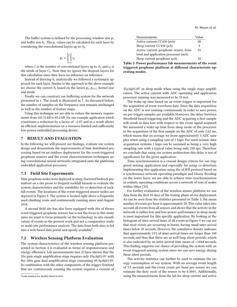
Name Type Kernel Stride Input sizeC0 Conv2D + ReLU 3x3 1 24 x 64 x 1C1 Conv2D + ReLU 3x3 2 24 x 64 x 32D0 Dropout - - 12 x 32 x 32C2 Conv2D + ReLU 3x3 1 12 x 32 x 32C3 Conv2D + ReLU 3x3 2 12 x 32 x 32D1 Dropout - - 6 x 16 x 32C4 Conv2D + ReLU 3x3 1 6 x 16 x 32C5 Conv2D + ReLU 1x1 1 6 x 16 x 32D2 Dropout - - 6 x 16 x 32C6 Conv2D + ReLU 1x1 1 6 x 16 x 32Af Average (Frequency) 1x16 1 6 x 16 x 1At Average (Time) 6x1 1 6 x 1 x 1C7 Conv2D + Sigmoid 1x1 1 1 x 1 x 1O Output - - 1
Table 1: The structure of the convolutional neural networkusing 2D convolutional layers (Conv2D) with Rectified Lin-ear Units (ReLU) and dropout layers to reduce overfitting.Number of parameters 38,403.
values of the input buffer and first layer’s output that affect the finaloutput. We first calculate the red output, then we calculate the blueoutput. This idea is similar to the depth-first approach describedin [5]. However, additionally we will optimize for the temporalcharacteristics of our input data with a sophisticated bufferingsystem.
When calculating the red output we already calculated one in-termediate result required for the blue output (the point where thelocal receptive fields in the layer 1 output overlap). If we want tocalculate the blue output we see that we only need two values fromthe first layer’s output which have never been calculated before(highlighted in bold). By following the receptive field of these twovalues we find they depend on four values from the input buffer,among which are two values which have not been used before andtwowhich have been used for calculating the red output. Effectively,this means that we can calculate the output of the network by acombination of new input values, intermediate results and bufferedvalues.
Figure 6 illustrates this buffering concept for the same example.We use the following nomenclature: pi is the number of new inputvalues for layer Li ; bi is the number of buffered input values forlayer Li ; po and bo are the respective output values. We call thearray of size pi the processing window of Li and the array of sizebi the buffer of layer Li . The value si is the stride for layer Li .The figure presents the last two time steps tn−2 and tn , whichresults in calculating the blue value in Figure 5. Based on Figure 5we set p0 = p1 = 2, po = 1 and b0 = 2,b1 = bo = 1. We nowapply the convolutional layer as before but on the reduced inputwindow. Obviously, we can now shift the input step by step intothe buffering system and calculate the output of the convolutionalneural network. For each step we acquire two new input samplesand discard two older input samples. This makes the bufferingsystem ideal for time series data as is the case in our applicationscenario. The memory requirement in Figure 6 compared to thecase in Figure 5 is reduced by 35% and the memory requirement for
0 0 1 01 1 1
0 11 1 0
2 0
W0
0 1 0
W1
1 1 0Layer L1
Stride 2
Layer L0
Stride 1
L0Input
L1Input
Output
tn-4 tn-2 tntn-6
Figure 5: The receptive field of the output values is illus-trated in red and in blue and grows with the number of lay-ers. The values are calculated layer by layer by convolvingthe layer input with the respective kernelw .
p0L0
b0 p1b1L1
pobo
tn-2 0
0tn -
11 0
0 1
1 01
0 0 1 0
2-
2
w0 w1
...
Figure 6: Illustration of the buffering concept: Each input ofa layer consists of one processing window (green) and onebuffer (yellow). Shown are two timesteps tn−2 and tn . Eachtimestep a new input is placed in the processing buffer oflayer L0. Subsequently, the the layers perform the convolu-tions followed by a left-shift of the processing window bytwo values.
each step is constant. The following section addresses the questionshow this general concept is transferred to our application specificconvolutional neural network introduced in Section 5.3 and howthe correct size of each layers’ buffers is determined.
6.1 Buffer System DesignClosely examining the inputs of our convolutional neural networkin Table 1 we see that it consists of 24 timesteps of a 64 value vector.The buffering concept can be expanded to this case if we assumeb0x64x1 and p0x64x1 input buffers. Similarly it can be expanded tomultiple feature maps (in our case 32) for the intermediate buffers.Before determining the actual buffer sizes we need to determine upto which layer the buffering concept is applicable. The last threelayers of the network are average pooling operations and scaling.The output of the time average pooling layer At is influenced byevery value of the 24x64x1 network input, which means that afterthis layer the buffering concept cannot be applied anymore. Wecan however calculate for each step one of the 6 input values toAt independently and place them in a buffer. Therefore we canconsider all layers up to At for the buffer system.
M. Meyer et al.
The buffer system is defined by the processing window size piand buffer size bi . The pi values can be calculated for each layer byconsidering the convolutional layers up to At .
pi =L−1∏l=i
sl
where L is the number of convolutional layers up to At and sl isthe stride of layer Cl . Note that we ignore the dropout layers forthis calculation since they have no influence on inference.
Instead of deriving bi analytically we followed a systematic ap-proach for each layer. Similar to the approach in the above examplewe choose the correct bi based on the layers pi , pi+1, kernel sizeand stride.
Finally we can construct our buffering system for the networkpresented in 1. The result is illustrated in 7. As discussed before,the number of samples on the frequency axis remains unchangedas well as the number of feature maps.
Using this technique we are able to reduce the memory require-ments from 245.76 kB to 85.6 kB for our example application whichconstitutes a reduction by a factor of ∼2.87 and as a result allowsan efficient implementation on a resource-limited and sufficientlylow-power embedded processing device.
7 RESULT AND EVALUATIONIn the following we will present our findings, evaluate our systemdesign and demonstrate the improvements of time distributed pro-cessing based on an outdoor deployment for the event-triggeredgeophone sensors and the event characterization techniques us-ing convolutional neural networks integrated onto the platformsembedded application processor.
7.1 Field Site ExperimentsNine geophone nodes were deployed in steep, fractured bedrock per-mafrost on a site prone to frequent rockfall hazards to evaluate thesystem characteristics and the suitability for co-detection of rock-fall events. The locations of the event-triggered sensor nodes aredepicted in Figure 8. The system is located right above a frequentlyused climbing route and continuously running since mid-August2018.
A second field site has also been equipped with 20x of thesesevent-triggered geophone sensors but is not the focus in this studysince we want to focus primarily on the technology in-situ classifi-cation of events in the present work and not a comparative studyor multi-site performance analysis. The data from both sites is fedinto a web-based data portal and openly available2.
7.2 Wireless Sensing Platform EvaluationThe system characteristics of the wireless sensing platform pre-sented in Section 4 is evaluated in terms of responsiveness andenergy efficiency. Lab measurements (see 2) have shown that the20x gain single amplification stage requires only 29µ[email protected] withthe 200x gain dual amplification stage consuming 49.9µ[email protected] .In combination with the other components of the trigger frontendthat are continuously running the system requires a current of
2Link omitted for double-blind review.
Measurements ValueActive current CC430 (mA) 28Sleep current CC430 (µA) 5Active current geophone sensor, fron-tend and application processor (mA)
35
Sleep current geophone (µA) 35Table 2: Power performance lab measurements of the eventtriggered geophone platform at different characteristic op-erating modes.
35µ[email protected] in sleep mode when using the single stage amplifi-cation. The active current with ADC operating and applicationprocessor running was measured to be 35 mA.
The wake-up time based on an event trigger is important forthe acquisition of event waveform data. Since the data acquisitionon the ADC is not running continuously in order to save power,no pre-trigger samples are available.Moreover, the delay betweenthreshold-based triggering and the ADC acquiring a first samplewill result in data loss with respect to the event signal acquired.We measured a wake-up time from sleep mode of the processorto the acquisition of the first sample on the ADC of only 2.62 ms,which means that on average we loose approximately 3 ADC sam-ples when using a sampling rate of 1 ksps. For most seismic dataacquisition systems 1 ksps can be assumed as being a very highsampling rate with a typical value being only 250 sps. Thereforewe conclude that using our system architecture this delay is not ofsignificance for the given application.
Time synchronization is a crucial design criteria for our trig-gered sensing application and especially for using co-detection.Implementing this application using the eLWB protocol based ona synchronous network operating paradigm and Glossy floodingon the lower layer, we are able to achieve time synchronizationin realistic operating conditions across a network of tens of nodeswithin 200µs [32].
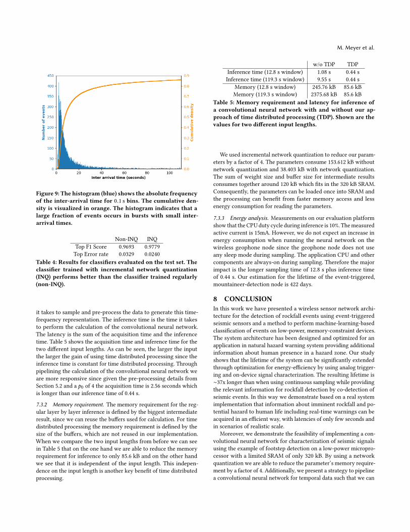
For further evaluation of the wireless sensor platform we usedata from the first 43 days of the testing phase of our deployment.As can be seen from the statistics presented in Table 3, the meannumber of events per hour is approximately 28. This value takes intoaccount all events from all sensors and shows that the activity in thenetwork is rather low and low-power performance in sleep modeis most important for this specific application. By looking at thehistogram of inter-arrival times of all events in Figure 9 we can seethat most events are occurring in bursts, having small inter-arrivaltimes below 20 seconds. However, the cumulative density indicatesthat approximately 15% of inter-arrival times are larger than 100seconds and thus that there are as well long silent periods, whichis also indicated by an inter-arrival time mean of ∼1044 seconds.This finding supports our choice of providing the system with anevent-triggered sensing system since we can save energy duringthese silent periods.
The activity statistics can further be used to estimate the en-ergy consumption of our system. With an average event lengthof 3.5 seconds and the event count per hour per sensor we canestimate the duty cycle of the sensor to be 0.304%. Additionally,using the measurements from the lab for sleep current and active

Event-triggered Natural Hazard Monitoringwith Convolutional Neural Networks on the Edge
64
b0
64
32
32
32
32
32
1632
16
32
16
32
16 1
C0 C1 C2 C3 C4 C5 C6 Af At C7
42 41 22 22 12 1 1 1 15 1 1p0 b1 p1 b2 p2 b3 p3 b4 p4 p5 p6 pf bt pts0 s1 s2 s3 s4 s5 s6
1 2 1 2 1 1 1
Figure 7: Illustrates the buffering architecture for the network from Table 1 with input size of 4x64x1. The input and outputof the network are depicted as well as the intermediate results of each layer. C0 to C7 are the convolutional layers. Af and Atare the average pooling layers for frequency and time, respectively.
Figure 8: Field site overview. Shown are the locations of theninewireless geophone sensor nodes. The base station to col-lect data and transmit it to a data backend is located behindthe little tower visible at the upper lefthand corner of the im-age. The scarp lies above a frequently used climbing route.
current we can calculate the average current of one sensor node tobe 0.986 mA. Using a battery of 13 Ah we can estimate the lifetimeof one sensor node to be 549 days.
Using the event triggered sensor around 788 kB are recorded onaverage every day. Continuous sampling with one of our sensorswould produce approx. 259 MB of data per day and sensor, which isan increase by a factor of ∼328. Similarly, assuming the geophone iscontinuously on and the communication processor sends packets asbefore, the estimated lifetime would be reduced by ∼95% to 15 daysexcluding effects of higher bandwidth requirements and networkcongestion that would inevitably occur when building on the samewireless subsystem.
Statistic ValueNumber of Sensors 9Days in Field 43Total Sensor On-Time (h) 28.227Total Number of Events 29040Mean Number of Events per Hour 28.14Mean Event Length (s) 3.5Mean Daily Acquisition Per Sensor (kB) 788Mean On-Time Per Hour Per Sensor (s) 10.941Mean Events per Hour Per Sensor 3.127Sensor duty cycle (%) 0.304Average current CC430 (mA) 0.845Average current geophone (mA) 0.141Average current total (mA) 0.986Energy per day (mAh) 23.667Battery (Ah) 13Estimated lifetime (days) 549
Table 3: The first 43 days of the test phase at our field sitehave been used to collect statistics about the system be-haviour. These statistics plus lab measurements have beenused to estimate the average current of a sensor node andits expected lifetime.
7.3 Time Distributed Processing EvaluationThe test results for the convolutional neural network from Section 5are depicted in Table 4. The error rate on the test set for the non-quantized network is 0.0329 and the F1 Score 0.9693. These resultsare slightly worse than the test error rate after quantization, whichis 0.0240 and the F1 score is 0.9779. The effect that quantizationimproves the test error rate has been also been observed by theauthors of the algorithm.
To underline the benefit of time distributed processing we com-pare the memory requirement and the latency of CNN inference fortwo scenarios: (i) inference of a 12.8 seconds window (which is thelength of the window used for network training) and (ii) inferenceof an approximately 2 minute long window (the maximum windowlength we can train with the given dataset).
7.3.1 Latency. The convolutional neural network must process atime-frequency representation of a specific size, in our case 24x64x1values, to perform one classification. The acquisition time is the time
M. Meyer et al.
Figure 9: The histogram (blue) shows the absolute frequencyof the inter-arrival time for 0.1 s bins. The cumulative den-sity is visualized in orange. The histogram indicates that alarge fraction of events occurs in bursts with small inter-arrival times.
Non-INQ INQTop F1 Score 0.9693 0.9779Top Error rate 0.0329 0.0240
Table 4: Results for classifiers evaluated on the test set. Theclassifier trained with incremental network quantization(INQ) performs better than the classifier trained regularly(non-INQ).
it takes to sample and pre-process the data to generate this time-frequency representation. The inference time is the time it takesto perform the calculation of the convolutional neural network.The latency is the sum of the acquisition time and the inferencetime. Table 5 shows the acquisition time and inference time for thetwo different input lengths. As can be seen, the larger the inputthe larger the gain of using time distributed processing since theinference time is constant for time distributed processing. Throughpipelining the calculation of the convolutional neural network weare more responsive since given the pre-processing details fromSection 5.2 and a p0 of 4 the acquisition time is 2.56 seconds whichis longer than our inference time of 0.44 s.
7.3.2 Memory requirement. The memory requirement for the reg-ular layer by layer inference is defined by the biggest intermediateresult, since we can reuse the buffers used for calculation. For timedistributed processing the memory requirement is defined by thesize of the buffers, which are not reused in our implementation.When we compare the two input lengths from before we can seein Table 5 that on the one hand we are able to reduce the memoryrequirement for inference to only 85.6 kB and on the other handwe see that it is independent of the input length. This indepen-dence on the input length is another key benefit of time distributedprocessing.
w/o TDP TDPInference time (12.8 s window) 1.08 s 0.44 sInference time (119.3 s window) 9.55 s 0.44 s
Memory (12.8 s window) 245.76 kB 85.6 kBMemory (119.3 s window) 2375.68 kB 85.6 kB
Table 5: Memory requirement and latency for inference ofa convolutional neural network with and without our ap-proach of time distributed processing (TDP). Shown are thevalues for two different input lengths.
We used incremental network quantization to reduce our param-eters by a factor of 4. The parameters consume 153.612 kB withoutnetwork quantization and 38.403 kB with network quantization.The sum of weight size and buffer size for intermediate resultsconsumes together around 120 kB which fits in the 320 kB SRAM.Consequently, the parameters can be loaded once into SRAM andthe processing can benefit from faster memory access and lessenergy consumption for reading the parameters.
7.3.3 Energy analysis. Measurements on our evaluation platformshow that the CPU duty cycle during inference is 10%. Themeasuredactive current is 15mA. However, we do not expect an increase inenergy consumption when running the neural network on thewireless geophone node since the geophone node does not useany sleep mode during sampling. The application CPU and othercomponents are always-on during sampling. Therefore the majorimpact is the longer sampling time of 12.8 s plus inference timeof 0.44 s. Our estimation for the lifetime of the event-triggered,mountaineer-detection node is 422 days.
8 CONCLUSIONIn this work we have presented a wireless sensor network archi-tecture for the detection of rockfall events using event-triggeredseismic sensors and a method to perform machine-learning-basedclassification of events on low-power, memory-constraint devices.The system architecture has been designed and optimized for anapplication in natural hazard warning system providing additionalinformation about human presence in a hazard zone. Our studyshows that the lifetime of the system can be significantly extendedthrough optimization for energy-efficiency by using analog trigger-ing and on-device signal characterization. The resulting lifetime is∼37x longer than when using continuous sampling while providingthe relevant information for rockfall detection by co-detection ofseismic events. In this way we demonstrate based on a real systemimplementation that information about imminent rockfall and po-tential hazard to human life including real-time warnings can beacquired in an efficient way, with latencies of only few seconds andin scenarios of realistic scale.
Moreover, we demonstrate the feasibility of implementing a con-volutional neural network for characterization of seismic signalsusing the example of footstep detection on a low-power micropro-cessor with a limited SRAM of only 320 kB. By using a networkquantization we are able to reduce the parameter’s memory require-ment by a factor of 4. Additionally, we present a strategy to pipelinea convolutional neural network for temporal data such that we can
Event-triggered Natural Hazard Monitoringwith Convolutional Neural Networks on the Edge
reduce the inference-time and the inference-memory requirementand keep them constant independent of the temporal size of theconvolutional neural network input.
REFERENCES[1] Martín Abadi, Ashish Agarwal, Paul Barham, Eugene Brevdo, Zhifeng Chen,
Craig Citro, Greg S. Corrado, Andy Davis, Jeffrey Dean, Matthieu Devin, San-jay Ghemawat, Ian Goodfellow, Andrew Harp, Geoffrey Irving, Michael Isard,Yangqing Jia, Rafal Jozefowicz, Lukasz Kaiser, Manjunath Kudlur, Josh Levenberg,Dandelion Mané, Rajat Monga, Sherry Moore, Derek Murray, Chris Olah, MikeSchuster, Jonathon Shlens, Benoit Steiner, Ilya Sutskever, Kunal Talwar, PaulTucker, Vincent Vanhoucke, Vijay Vasudevan, Fernanda Viégas, Oriol Vinyals,Pete Warden, Martin Wattenberg, Martin Wicke, Yuan Yu, and Xiaoqiang Zheng.2015. TensorFlow: Large-Scale Machine Learning on Heterogeneous Systems.(2015). Software available from tensorflow.org.
[2] D. Amitrano, J. R Grasso, and G. Senfaute. 2005. Seismic Precursory Patternsbefore a Cliff Collapse and Critical Point Phenomena. Geophysical ResearchLetters 32, 8 (April 2005), L08314. https://doi.org/10.1029/2004GL022270
[3] S. Anchal, B. Mukhopadhyay, and S. Kar. 2018. UREDT: Unsupervised LearningBased Real-Time Footfall Event Detection Technique in Seismic Signal. IEEE Sen-sors Letters 2, 1 (March 2018), 1–4. https://doi.org/10.1109/LSENS.2017.2787611
[4] R. Andri, L. Cavigelli, D. Rossi, and L. Benini. 2018. YodaNN: An Architecturefor Ultralow Power Binary-Weight CNN Acceleration. IEEE Transactions onComputer-Aided Design of Integrated Circuits and Systems 37, 1 (Jan. 2018), 48–60.https://doi.org/10.1109/TCAD.2017.2682138
[5] Jonathan Binas and Yoshua Bengio. 2018. Low-Memory Convolutional NeuralNetworks through Incremental Depth-First Processing. arXiv:1804.10727 [cs](April 2018). arXiv:cs/1804.10727
[6] E. Cakir, T. Heittola, H. Huttunen, and T. Virtanen. 2015. Polyphonic Sound EventDetection Using Multi Label Deep Neural Networks. In 2015 International JointConference on Neural Networks (IJCNN). 1–7. https://doi.org/10.1109/IJCNN.2015.7280624
[7] Emre Cakir, Giambattista Parascandolo, Toni Heittola, Heikki Huttunen, TuomasVirtanen, Emre Cakir, Giambattista Parascandolo, Toni Heittola, Heikki Huttunen,and Tuomas Virtanen. 2017. Convolutional Recurrent Neural Networks forPolyphonic Sound Event Detection. IEEE/ACM Trans. Audio, Speech and Lang.Proc. 25, 6 (June 2017), 1291–1303. https://doi.org/10.1109/TASLP.2017.2690575
[8] Y. Chen, T. Krishna, J. S. Emer, and V. Sze. 2017. Eyeriss: An Energy-EfficientReconfigurable Accelerator for Deep Convolutional Neural Networks. IEEEJournal of Solid-State Circuits 52, 1 (Jan. 2017), 127–138. https://doi.org/10.1109/JSSC.2016.2616357
[9] Keunwoo Choi, György Fazekas, Kyunghyun Cho, and Mark Sandler. 2017. AComparison of Audio Signal Preprocessing Methods for Deep Neural Networkson Music Tagging. arXiv:1709.01922 [cs] (Sept. 2017). arXiv:cs/1709.01922
[10] François Chollet and others. 2015. Keras. Python Framework (2015). Softwareavailable from keras.io.
[11] C. Colombero, C. Comina, S. Vinciguerra, and P. M. Benson. 2018. Microseis-micity of an Unstable Rock Mass: From Field Monitoring to Laboratory Testing.Journal of Geophysical Research: Solid Earth (Feb. 2018). https://doi.org/10.1002/2017JB014612
[12] Jerome Faillettaz, Dani Or, and Ingrid Reiweger. 2016. Codetection of Acous-tic Emissions during Failure of Heterogeneous Media: New Perspectives forNatural Hazard Early Warning: CODETECTION OF ACOUSTIC EMISSIONS.Geophysical Research Letters 43, 3 (Feb. 2016), 1075–1083. https://doi.org/10.1002/2015GL067435
[13] L. Girard, J. Beutel, S. Gruber, J. Hunziker, R. Lim, and S. Weber. 2012. A CustomAcoustic Emission Monitoring System for Harsh Environments: Application toFreezing-Induced Damage in Alpine Rock Walls. Geoscientific Instrumentation,Methods and Data Systems 1, 2 (2012), 155–167.
[14] Thomas Glade, Malcolm Anderson, and Michael J. Crozier. 2005. LandslideHazard and Risk. John Wiley & Sons, Ltd, Chichester, West Sussex, England.https://doi.org/10.1002/9780470012659
[15] Kartik Hegde, Jiyong Yu, Rohit Agrawal, Mengjia Yan, Michael Pellauer, andChristopher W. Fletcher. 2018. UCNN: Exploiting Computational Reuse inDeep Neural Networks via Weight Repetition. arXiv:1804.06508 [cs] (April 2018).arXiv:cs/1804.06508
[16] Shawn Hershey, Sourish Chaudhuri, Daniel P. W. Ellis, Jort F. Gemmeke, ArenJansen, R. Channing Moore, Manoj Plakal, Devin Platt, Rif A. Saurous, BryanSeybold, Malcolm Slaney, Ron J. Weiss, and Kevin Wilson. 2016. CNN Archi-tectures for Large-Scale Audio Classification. arXiv: 1609.09430 (Sept. 2016).arXiv:1609.09430
[17] Emanuele Intrieri, Giovanni Gigli, Francesco Mugnai, Riccardo Fanti, and NicolaCasagli. 2012. Design and Implementation of a Landslide Early Warning System.Engineering Geology 147-148 (Oct. 2012), 124–136. https://doi.org/10.1016/j.enggeo.2012.07.017
[18] Akhil Mathur, Nicholas D. Lane, Sourav Bhattacharya, Aidan Boran, ClaudioForlivesi, and Fahim Kawsar. 2017. DeepEye: Resource Efficient Local Execu-tion of Multiple Deep Vision Models Using Wearable Commodity Hardware.In Proceedings of the 15th Annual International Conference on Mobile Systems,Applications, and Services (MobiSys ’17). ACM, New York, NY, USA, 68–81.https://doi.org/10.1145/3081333.3081359
[19] Bradley McDanel, Surat Teerapittayanon, and H. T. Kung. 2017. Embedded Bina-rized Neural Networks. arXiv:1709.02260 [cs] (Sept. 2017). arXiv:cs/1709.02260
[20] Matthias Meyer and Samuel Weber. 2018. Code For Classifier Training AndEvaluation Using The Micro-Seismic And Image Dataset Acquired At MatterhornHörnligrat, Switzerland. https://doi.org/10.5281/zenodo.1321176
[21] Matthias Meyer, Samuel Weber, Jan Beutel, Stephan Gruber, Tonio Gsell, AndreasHasler, and Andreas Vieli. 2018. Micro-Seismic And Image Dataset Acquired AtMatterhorn Hörnligrat, Switzerland. https://doi.org/10.5281/zenodo.1320834
[22] Matthias Meyer, Samuel Weber, Jan Beutel, and Lothar Thiele. 2018. SystematicIdentification of External Influences in Multi-Year Micro-Seismic RecordingsUsing Convolutional Neural Networks. Earth Surface Dynamics Discussions (Aug.2018), 1–24. https://doi.org/10.5194/esurf-2018-60 In review.
[23] C. Occhiena, V. Coviello, M. Arattano, M. Chiarle, U. Morra di Cella, M. Pirulli, P.Pogliotti, and C. Scavia. 2012. Analysis of Microseismic Signals and TemperatureRecordings for Rock Slope Stability Investigations in High Mountain Areas. Nat.Hazards Earth Syst. Sci. 12, 7 (July 2012), 2283–2298. https://doi.org/10.5194/nhess-12-2283-2012
[24] Patrick Paitz, Alexey Gokhberg, and Andreas Fichtner. 2018. A Neural Networkfor Noise Correlation Classification. Geophysical Journal International 212, 2 (Feb.2018), 1468–1474. https://doi.org/10.1093/gji/ggx495
[25] Shijia Pan, Ningning Wang, Yuqiu Qian, Irem Velibeyoglu, Hae Young Noh,and Pei Zhang. 2015. Indoor Person Identification Through Footstep InducedStructural Vibration. In Proceedings of the 16th International Workshop on MobileComputing Systems and Applications (HotMobile ’15). ACM, New York, NY, USA,81–86. https://doi.org/10.1145/2699343.2699364
[26] Thibaut Perol, Michaël Gharbi, and Marine Denolle. 2018. Convolutional NeuralNetwork for Earthquake Detection and Location. Science Advances 4, 2 (Feb.2018), e1700578. https://doi.org/10.1126/sciadv.1700578
[27] Tara N. Sainath, Ron J. Weiss, Andrew Senior, KevinW.Wilson, and Oriol Vinyals.2015. Learning the Speech Front-End With Raw Waveform CLDNNs. In Proc.Interspeech.
[28] G. Senfaute, A. Duperret, and J. A. Lawrence. 2009. Micro-Seismic PrecursoryCracks Prior to Rock-Fall on Coastal Chalk Cliffs: A Case Study at Mesnil-Val,Normandie, NW France. Natural Hazards and Earth System Sciences 9 (Oct. 2009),1625–1641.
[29] Thomas Spillmann, Hansruedi Maurer, Alan G. Green, Björn Heincke, HeikeWillenberg, and Stephan Husen. 2007. Microseismic Investigation of an UnstableMountain Slope in the Swiss Alps. Journal of Geophysical Research 112, B7 (July2007). https://doi.org/10.1029/2006JB004723
[30] Jost Tobias Springenberg, Alexey Dosovitskiy, Thomas Brox, and Martin Ried-miller. 2014. Striving for Simplicity: The All Convolutional Net. arXiv:1412.6806[cs] (Dec. 2014). arXiv:cs/1412.6806
[31] Nitish Srivastava, Geoffrey Hinton, Alex Krizhevsky, Ilya Sutskever, and RuslanSalakhutdinov. 2014. Dropout: A Simple Way to Prevent Neural Networks fromOverfitting. J. Mach. Learn. Res. 15, 1 (Jan. 2014), 1929–1958.
[32] Felix Sutton, Reto Da Forno, Jan Beutel, and Lothar Thiele. 2017. BLITZ: ANetwork Architecture for Low Latency and Energy-Efficient Event-TriggeredWireless Communication. In Proceedings of the 4th ACM Workshop on Hot Topicsin Wireless (HotWireless ’17). ACM, New York, NY, USA, 55–59. https://doi.org/10.1145/3127882.3127883
[33] Felix Sutton, Reto Da Forno, David Gschwend, Tonio Gsell, Roman Lim, JanBeutel, and Lothar Thiele. 2017. The Design of a Responsive and Energy-EfficientEvent-Triggered Wireless Sensing System. In Proceedings of the 2017 InternationalConference on Embedded Wireless Systems and Networks (EWSN ’17). JunctionPublishing, USA, 144–155.
[34] Felix Sutton, Marco Zimmerling, Reto Da Forno, Roman Lim, Tonio Gsell, GeorgiaGiannopoulou, Federico Ferrari, Jan Beutel, and Lothar Thiele. 2015. Bolt: AStateful Processor Interconnect. In Proceedings of the 13th ACM Conference onEmbedded Networked Sensor Systems (SenSys ’15). ACM, New York, NY, USA,267–280. https://doi.org/10.1145/2809695.2809706
[35] Naoya Takahashi, Michael Gygli, Beat Pfister, and Luc Van Gool. 2016. DeepConvolutional Neural Networks and Data Augmentation for Acoustic EventRecognition. In Proc. Interspeech 2016. San Fransisco.
[36] Theodoros D. Verykios, Domenico Balsamo, and Geoff V. Merrett. 2018. SelectivePolicies for Efficient State Retention in Transiently-Powered Embedded Systems:Exploiting Properties of NVM Technologies. Sustainable Computing: Informaticsand Systems (July 2018). https://doi.org/10.1016/j.suscom.2018.07.003
[37] G. Werner-Allen, J. Johnson, M. Ruiz, J. Lees, and M. Welsh. 2005. MonitoringVolcanic Eruptions with a Wireless Sensor Network. In Proceeedings of the SecondEuropean Workshop on Wireless Sensor Networks, 2005. 108–120. https://doi.org/10.1109/EWSN.2005.1462003

M. Meyer et al.
[38] GeoffWerner-Allen, Konrad Lorincz, Jeff Johnson, Jonathan Lees, andMattWelsh.2006. Fidelity and Yield in a Volcano Monitoring Sensor Network. In Proceedingsof the 7th Symposium on Operating Systems Design and Implementation (OSDI ’06).USENIX Association, Berkeley, CA, USA, 381–396.
[39] J. Wu, C. Leng, Y. Wang, Q. Hu, and J. Cheng. 2016. Quantized ConvolutionalNeural Networks for Mobile Devices. In 2016 IEEE Conference on Computer Visionand Pattern Recognition (CVPR). 4820–4828. https://doi.org/10.1109/CVPR.2016.521
[40] Yundong Zhang, Naveen Suda, Liangzhen Lai, and Vikas Chandra. 2017. HelloEdge: Keyword Spotting on Microcontrollers. arXiv:1711.07128 [cs, eess] (Nov.2017). arXiv:cs, eess/1711.07128
[41] Aojun Zhou, Anbang Yao, Yiwen Guo, Lin Xu, and Yurong Chen. 2017. Incremen-tal Network Quantization: Towards Lossless CNNs with Low-Precision Weights.arXiv:1702.03044 [cs] (Feb. 2017). arXiv:cs/1702.03044