This content has been downloaded from IOPscience. Please scroll down to see the full text.

Download details:

IP Address: 129.169.70.132

This content was downloaded on 12/05/2016 at 11:56

Please note that terms and conditions apply.

Eversion of bistable shells under magnetic actuation: a model of nonlinear shapes

View the table of contents for this issue, or go to the journal homepage for more

2016 Smart Mater. Struct. 25 065010

(http://iopscience.iop.org/0964-1726/25/6/065010)

Home Search Collections Journals About Contact us My IOPscience

Eversion of bistable shells under magneticactuation: a model of nonlinear shapes

Keith A Seffen1 and Stefano Vidoli2

1Advanced Structures Group, Department of Engineering, University of Cambridge, UK2Department of Structural and Geotechnical Engineering, Sapienza University of Rome, Italy

E-mail: kas14@cam.ac.uk

Received 14 October 2015, revised 27 January 2016Accepted for publication 22 March 2016Published 11 May 2016

AbstractWe model in closed form a proven bistable shell made from a magnetic rubber compositematerial. In particular, we incorporate a non-axisymmetrical displacement field, and we capturethe nonlinear coupling between the actuated shape and the magnetic flux distribution around theshell. We are able to verify the bistable nature of the shell and we explore its eversion duringmagnetic actuation. We show that axisymmetrical eversion is natural for a perfect shell but thatnon-axisymmetrical eversion rapidly emerges under very small initial imperfections, as observedin experiments and in a computational analysis. We confirm the non-uniform shapes of shell andwe study the stability of eversion by considering how the landscape of total potential andmagnetic energies of the system changes during actuation.

Keywords: bistable, shell, magnetic, actuation, eversion

(Some figures may appear in colour only in the online journal)

1. Introduction

In an earlier paper [1], the first author, with others, consideredthe actuation capabilities of a novel magnetic rubber com-posite material for developing ‘active’ shape-changingstructures. The material was made into a stress-free, shallowcap, approximately 36 mm across, which was then supportedcentrally in a convex manner. When a strong magnet wasbrought closer to the cap along its axis, the cap eventually‘everted’ at a separation of 13 mm, and remained inside outafter the magnet was removed, see figure 1. The cap shape isclearly uneven during eversion, only becoming axisymme-trical again at the end. A finite element analysis was con-ducted to confirm the proximity threshold for eversion, theshape of cap during eversion, and the final resting shape. Asequence of these shapes is repeated in figure 1 along with thevariation of elastic strain energy over time, with some unusualfeatures that are discussed later.

Finite element analysis reveals behaviour for a specificset-up, which may, or may not, be general. For broaderinsight, many analyses of different initial geometries areneeded but this can be time-consuming, and critical infor-mation is not revealed in closed form—essential for furtherdesign and development. For this, a theoretical model oflarge-displacement eversion is required; however, relevantframeworks of the time were inadequate. For example, theassumption of uniform curvature used in studies on multi-stable shells [2, 3] is clearly violated during eversion, whereasthe emerging linearly varying curvature (LVC) model [4]considered non-uniform shapes of shell but actuation effectsremained decoupled from the deformation they induced. Themagnetic field applied to the shell is spatially nonlinear, andthe level and distribution of actuation strains inherentlydepend on the shell displacements. Such strong coupling hasnot been modelled compactly, to our knowledge, and cap-turing this behaviour in finite element analysis was, in itself,non-trivial.

In this paper, we build a sophisticated theoretical modelwith non-uniform displacements and coupled magneticactuation by augmenting the LVC model from [4], in order tocompute the bistable shapes, to elucidate possible eversion

Smart Materials and Structures

Smart Mater. Struct. 25 (2016) 065010 (11pp) doi:10.1088/0964-1726/25/6/065010

Original content from this work may be used under the termsof the Creative Commons Attribution 3.0 licence. Any

further distribution of this work must maintain attribution to the author(s) andthe title of the work, journal citation and DOI.

0964-1726/16/065010+11$33.00 © 2016 IOP Publishing Ltd Printed in the UK1

‘paths’, and to explore how axisymmetry may be ‘lost’ duringeversion. The latter is not readily demonstrated by finiteelement analysis because the cap and magnetic field arenominally axisymmetrical; there has to be some kind ofimperfection present for the simulation to follow an alter-native equilibrium path of non-axisymmetrical shapes, see forexample [5]. This was achieved w.r.t. figure 1 by imposing asmall initial tilt of the cap about its pole relative to themagnetic field axis because of inevitable axial misalignmentsin practice. However, it is well known in perfectly symme-trical systems that symmetry-breaking behaviour can be thenorm, for example in beam arches and spherical caps underaxial point loads [6] and in vibrating shells [7]. In our model,we build this capability into the displacement field, whichallows us to ascertain whether or not symmetry is lost duringactuation under perfect conditions and to understand theinfluence that actuation has upon this assumption alongsidethe usual competing effects of bending and stretching inordinary shells. The layout of study is as follows.

We reformulate the LVC model using a displacementfield with axisymmetrical and antisymmetrical components.Their respective amplitudes are taken as control parametersand their expressions always ensure that the edge of the capis free from tractions. We follow the recognised proceduredeveloped originally in [2] and enhanced in [3] for findingequilibrium shapes: we find the in-plane stresses for thedeformed cap by solving Gauss’ compatibility equation—identical to one of the Föppl–von Kármán shallow plateequations; using these stresses and knowing the deformedcurvatures, we can compute the total elastic strain energystored in the deformed cap as functions of the controlparameters. The effect of the applied magnetic field isincorporated as a potential energy function, which is addedto the elastic components to yield the total energy of the

system. By exploring the total energy ‘landscape’ for a givenproximity of magnet, we can establish the nature of equili-bria and how they change as the magnet moves. We do notinclude dynamic or inertial behaviour because that is beyondour scope; our focus is the symmetry character of eversion,which is the same for all time and thus, is defined by thequasi-static response of the shell. Correspondingly, weverify that the shell in figure 1 is bistable and that its evertedshape is non-uniform. We show that the magnetic field, ifstrong enough, is able to render the natural configurationunstable i.e. to initiate eversion. We capture the evertedshape of shell when the magnet is close enough so thatcontact takes place between the two. We confirm the generalstrain energy profile from finite element analysis shown infigure 1, and that the eversion threshold is nonlinearlydependent on the initial title angle; moreover, we predict thesame threshold as per finite element analysis. We then makesome general conclusions.

2. Elastic energy: an approximation with twodegrees of freedom

2.1. Kinematical assumptions

Consider a thin shallow shell with a circular planform ofradius R, planform area p=A R2, and constant thickness te.Using cylindrical coordinates ( )r f z, , , the natural stress-freeconfiguration, 0, is identified by the shell mid-surfacecoordinate, w0, in the transverse direction, ζ, with

{( ( )) }

( ) ≔( )

r f z r r f p

rr

= = <w R

wR

, , , 0 , 0 2 ,

2.

1

0 0

0

2

c

Figure 1. Left top: high speed capture of the actuation of a bistable rubber magnetic cap from [1]. The cap is 1.5 mm thick, approximately36 mm wide, and is held at its centre. The magnet is moved closer to the cap and, at an axial distance of around 13 mm from the cap centre,the cap everts unevenly—without axisymmetry—before making contact with the magnet. When the magnet is retracted, the cap remainseverted. Left bottom and right: finite element analysis shows a non-axisymmetrical transition for the cap when it is initially tilted by 5°relative to the magnetic axis: the time taken is around 0.1 s. The plot indicates the elastic strain energy of deformation during the transitionfor two axial distances: d=13 mm, which results in eversion; d=14 mm, which does not. The feature highlighted in the red box isconfirmed later.

2

Smart Mater. Struct. 25 (2016) 065010 K A Seffen and S Vidoli

This is a doubly curved, axisymmetrical shape with uniformand positive Gaussian curvature, R1 c

2, as per the stress-freecap in figure 1. If the shell is sufficiently curved and thin, ithas one other stable, everted configuration, at least. A simplecondition for bistability is derived in [4] for shallow isotropicshells: that the dimensionless ratio, ≔l R t Ac e , is less than acritical ratio, l 0.04c . We also assume material isotropyand linear elastic behaviour.

Every shell configuration,

{( ˆ ( )) }( )

r f z r f r f p= = <w R, , , , 0 , 0 2 ,2

must satisfy the following boundary conditions on its edge atr = R:

( ˆ ) ( )r

¶ -¶

=r=

w wa0, 3

R

20

2

[ ]

( ˆ ) ( ˆ ) ( ˆ ) ∣

( )

r r r r r

f p

¶ -¶

+¶ -

¶-

¶ -¶

=

" Î

r=⎛⎝⎜

⎞⎠⎟

w w w w w w

b

1 10,

0, 2 .

3

R

30

3

20

2 20

Equation (3a) imposes a vanishing bending moment whileequation (3b) enforces a vanishing shear force. The lowest-order polynomial in ρ that can be selected to satisfy them is

ˆ ( ) ( )rr r r r

= - + -wR

s

R

s

R R

s

R R2

5

4

15

32

5

48. 4s

2

c

2

c

4

2c

6

4c

As the scalar parameter s varies, ˆ ( )rws describes a deformedaxisymmetrical shell with a free edge: clearly, the naturalconfiguration, equation (2), is recovered when s= 0. For>s 0, eversion is deemed to be occurring when the curvature

at the cap centre (r = 0), given by

ˆr

¶¶

=-

r=

w s

R

2 5

2,

2s

20 c

changes sign, i.e. when >s 0.4.

Antisymmetrical distortions are addressed by com-plementing equation (4) with a second ansatz of circumfer-ential variation. We find the simplest form to be:

ˆ ( ) ( )r fr r r

f=- -⎛

⎝⎜⎞⎠⎟w t

R R

R R,

9 2 24

34cos , 5t

4 2 6 4 2

4c

whose amplitude is governed by the scalar parameter t. Thefinal cosine term ensures that the shape wt has one maximumand one minimum, diametrically opposed and with ampli-tudes ( )t R R22

c , as seen in figure 1. Note that the functionˆ ( )r fw ,t has been carefully tuned in terms of ρ to satisfy

[ ]

ˆ

ˆ ˆ ˆ

( )

r

r r r r r

f p

¶¶

=

¶¶

+¶¶

-¶¶

=

" Î

r

r

=

=

⎛⎝⎜

⎞⎠⎟

w

w w w

0,

1 10,

0, 2 . 6

t

R

t t t

R

2

2

3

3

2

2 2

Hence, the general shape function

ˆ ( ) ˆ ( ) ˆ ( ) ( )r f r f r f= +w w w, , , , 7t ts, s

satisfies the boundary conditions, equation (3), for everychoice of s and t. Note that most shapes parameterised byequation (7) do not have a uniform curvature field.

2.2. Bending and stretching energies

For a deformed Föppl–von Kármán shell, the stored elasticstrain energy is the sum of two quadratic components inbending, b, and in stretching (or membranal), s. For thebending energy, see for instance [8], we have

[ ( ) · ( )] ( ) ò ò r r f= - -p

K K K K1

2d d , 8

R

b0

2

00 0

where ˆ= wK is the standard curvature field of deformedshell, equation (2), = wK0 0 is the curvature field of thenatural stress-free shape, equation (1), and is the bendingstiffness matrix for an isotropic material:

( ) n

nn

n= =

- -

⎛⎝⎜⎜

⎞⎠⎟⎟

t Yt

12,

1

1 01 0

0 0 1. 9e

2e

2

Y is the Young modulus and ν is the Poisson ratio. Usingequation (7), the standard components of K are

ˆ ˆ

( ) ( )

r r f r fr r f

=¶¶ ¶

-¶¶

=- +

rfKw w

R R t

R R

1 1

10 27 24 sin

34, 11

2

2

4 2 2 4

4c

ˆ ( ) ( ) ( )r

r r r r f=

¶¶

=- + - - - +

Kw R s s R s R R t

R R

765 425 68 2 5 48 5 9 4 cos

136, 10rr

2

2

2 2 4 4 4 2 2 4

4c

3

Smart Mater. Struct. 25 (2016) 065010 K A Seffen and S Vidoli

while K0 has components = =ffK K R1rr0 0 c and =fK 0r0 .The bending energy equation in equation (8) can be integratedin closed form to obtain

( )( )

[( )

( ) ] ( )

n

n

n

=-

+

+ -

s tY R t

Rs

t

,1

0.573 0.409

0.084 0.019 . 13

b

2e3

2c2

2

2

Note that ( ) s t,b vanishes for the natural configurationwhere = =s t 0.

Denoting the membranal stress field via N, the stretchingstrain energy has the general expression:

( · ) ( ) ò ò r r f=p

- N N1

2d d , 14

R

s0

2

0

1

where is the membranal stiffness defined in equation (9),see [8]. The membranal stress field can be found by solvingGauss’ original compatibility equation for shallow shelldisplacements because we already know the Gaussiancurvature properties of the shell; specifically, the differencein Gaussian curvature between the current and initial shapesconstitutes a ‘forcing’ function for Gauss’ equation. The mid-surface strains are substituted by stresses reformulated interms of an Airy function j for isotropic materials, andGauss’ equation, in its form defined in [4], now reads as

( ) ( )jDD = -Yt K Kdet det , on , 15e 0

with no in-plane tractions on the free edges demanding that

( )jj

=¶¶

= ¶n

0, on . 16

Here, jDD indicates the standard biharmonic operator on j,and ¶ ¶n indicates derivation with respect to the direction n,the outward normal to ¶ . The usual membranal stresscomponents per unit length are recovered, see for instance [9],from:

( )

rjr r

jf r r

jf

jr

=¶¶

+¶¶

= -¶¶

¶¶

=¶¶

rf

ff

⎛⎝⎜

⎞⎠⎟N N

N

1 1,

1,

. 17

rr 2

2

2

2

2

The forcing term in equation (15) can be computed in closedform from the generic shape variation in equation (7). Thisreturns

( ) ( )

( )

å å r f- =

= == =R

C s t k

a k

K Kdet det1

, cos ,

0, 2, 4, 6, 8, 0, 1, 2, 18k a

a ka

0c2

0

2

0

8

,

where the coefficients Ca k, are functions of s and t, given inthe appendix. Hence, the Airy function required to solveequation (15) is a linear combination of the solutions of 15elliptic problems after substituting equation (18) intoequation (15). These may be written individually as

( )

( )

j r f

jj

DD =

=¶¶

= ¶

k

n

cos , on

0, on 19

aka

akak

and each one can be solved in closed form to reveal:

( )( [ ( ) ( )])

( )( )( )( )( )

j r fr r r

f

=+ - - + - +

- + - + + + + +´

- + +R R R k a R a k

a k a k a k a kk

,

2 4 2

2 2 4 2 4cos .

ak

k a k a k4 2 2 2

The generic Airy function is correspondingly written

( ) ( )åj j r f=Yt

RC s t, ,

a ka k ak

e

c2

,,

and, using equations (14) and (17), the stretching strainenergy can be computed to be

2.3. Total elastic energy: evidence of bistability

The total elastic energy is the sum of the two components

( ) ( ) ( ) ( ) = +s t s t s t, , , 21e b s

and is a fourth order polynomial expression in s and t. We cansolve ( ) s t,e for stationary values of s and t, in order to findthe range of equilibria. We can also explore the variation of

( ) s t,e on the plane (s, t), where contours of strain energyprovide direct information about the stability of equilibria.This has been performed in figure 2 according to the values intable 1 for the shell in figure 1 from [1]:

Two energy minima corresponding to stable equilibriaare clearly evident: the natural, stress-free state is located at( ) ( )=s t, 0, 0 , and the everted configuration at

( ) ( )n

n n= ´ - - + + +

+ - + - +

⎛⎝⎜

⎞⎠⎟s t

Y R t

R

s s s t s t ss t s t t t t

,0.0835 0.183 0.0007 0.0091 0.1011

0.0007 0.0099 0.0001 0.0002 0.0014. 20s

6e

c4

4 3 2 2 2 2 2

2 2 4 2 2

ˆ ˆ ( ) ( ) ( )r f r r

r r r r f=

¶¶

+¶¶

=- - + - - +

ffKw w R R R s R R t

R R

1 1 136 85 3 4 4 10 27 24 cos

136, 12

2

2

2

4 4 2 2 4 4 2 2 4

4c

4

Smart Mater. Struct. 25 (2016) 065010 K A Seffen and S Vidoli

( ) ( )=s t, 0.995, 0 . The latter is axisymmetrical becauset=0 and has non-uniform curvature, as shown. Bistability isalso confirmed by calculating ( )l l= < 0.0255 0.04c .Elsewhere on the landscape, the deformed shell is not stableand must ‘move’ towards either stable equilibria along a pathof steepest descent—a longstanding principle embodied, forexample, in the behaviour of chemical reactions [10]. When

actuating forces are present, the landscape itself is not staticbut is modified by the work contribution from actuation—asdescribed in, for example, [11, 12]. We must therefore con-sider the total energy landscape including the magneticpotential energy, expressed in terms of the shape of shell, i.e.as a function of s and t.

Figure 2. Top: contour plot of the elastic strain energy, e on the plane (s, t), where s and t are control parameters measuring the degree ofaxisymmetry and antisymmetry, respectively. The two minima are marked by heavy red points: the initial state at the origin and the everted stated at( ) ( )=s t, 0.995, 0 . The orange points indicate a path of axisymmetrical shell shapes between the minima; the blue dots is a non-axisymmetricalpath, which follows a path of least gradient up to saddle at ( ) ( )s t, 0.65, 1.8 , before descending towards the everted minimum. Bottom:corresponding non-axisymmetrical shapes and axisymmetrical shapes.

Figure 3. The elastic strain energy components along theaxisymmetrical path in figure 2: total strain energy, e (black solid);bending, b (grey dashed) and membranal, s (orange dashed)components.

Figure 4. Ratio U Us M between the energies needed for non-axisymmetrical and axisymmetrical eversion, plotted against thedimensionless ratio λ, for n = 0.2, 0.5, 0.8. The region l lc,where shallow shells are bistable, is shaded by a light gray colour; adashed line marks the actual value of λ for the shell underconsideration.

5

Smart Mater. Struct. 25 (2016) 065010 K A Seffen and S Vidoli

By gradually increasing the level of actuation—bymoving the magnet closer to the cap, we may observe how thestability character of the original elastic strain energy land-scape changes. Eversion begins when the natural configura-tion loses its stability margin and becomes unstable in thislandscape, leaving only the stable everted configuration. Thisis an important point, which is not usually noted in studies ofactuator effectiveness, but which has been discussedthoughtfully in [13]. In becoming unstable, the landscapearound the natural state changes from a well to a saddle, andeversion follows the path of steepest descent along a directionin which the local gradient first becomes negative. As notedbefore, we neglect inertial effects because this adds furthermodelling complexity; importantly, the properties of eversion,such as symmetry and threshold proximity, do not originate inthe dynamics of response.

Before formally calculating the magnetic potential energy,it is worth pondering how eversion may proceed without axi-symmetry. The magnetic field is axisymmetrical in nature and,therefore, exerts symmetrical forces upon the cap initially,provided the cap is itself perfectly axisymmetrical and isotropic.Although the actuator effect is absent from the landscape infigure 2, axisymmetrical deformation proceeds along t=0,along a path of steepest ascent and descent towards the evertedshape, as highlighted. Either side of the ascending path, thereare shape configurations for which e is immediately lowerand, intuitively, this part of the path not be globally stable. If, onthe other hand, we move along a different path, it may bepossible that local perturbations from e are stable, giving amore secure route for eversion; one such route is also high-lighted, which fulfils this property by rising least steeply awayfrom the natural state, where the distance between successivecontours is largest. Since t is now non-zero, the intermediateshapes of shell are non-axisymmetrical, as shown. If we nowcompute the following two energetic quantities:

1. ≔ ( ) =U s tmax , 0M s e , the maximum elastic energyencountered along the axisymmetric path;

2. ≔ ( )U s tmin max ,ts s e , the elastic energy associatedwith the saddle point with ¹t 0,

then the ratio U U 1s M measures, informally, the energe-tical advantage of the non-axisymmetrical transition withrespect to the axisymmetrical one; the smaller the value ofU Us M, the greater the tendency for non-axisymmetricaleversion under suitable perturbations.

For the model under consideration, the ratio U Us M canbe computed in closed form and turns out to be a functiononly of the Poisson ratio, ν, and the dimensionless parameter,

( )l p= R t Rc e2 , which measures the ratio between bending

and stretching energies according to l µ2b s. Figure 4

plots U Us M with respect to λ for different values of thePoisson ratio.

At larger values of the dimensionless parameter l lc,where bistability emerges, U Us M. However as soon as λ

decreases, U Us M becomes increasingly smaller. Eventually,for l 0, a plateau is reached where U U 0.36s M for anyvalue of the Poisson ratio. For our shell, we obtain

U U 0.9s M , signifying that axisymmetrical eversion ishighly likely; a quantitative answer is only conveyed whenwe understand how actuation and imperfections distort theoverall energy landscape, which is now performed.

3. Magnetic actuation

The magnetic field in [1] is generated by connecting togetherhigh-strength Neodymium N42 disk magnets along their axisinto a cylindrical stack for a more intense field of flux. Cal-culating the resulting field is not trivial but we follow thescheme outlined in [1], originally based on the derivationin [14].

The magnetic field, B, is assumed to be axisymmetrical,and to vary with radial distance, r, and axial distance, z, froma reference point source. More formally

( ) ( ) ( )= -Fr z r zB , , , 22m

where

( )

( )( )

( ) ( )( ) ( )

( )

mp

F

= - +-- +

- - + +-

- + +

⎡⎣⎢

⎛⎝⎜

⎞⎠⎟

⎛⎝⎜

⎞⎠⎟

⎤⎦⎥

r z

Ma r z E

a r

a r z

a r H z Ea r

a r H z

,

4

4,

23

m

0 2 22 2

2 22 2

is the magnetic potential originating from two parallel,oppositely charged monopolar disks of radius r=a separatedby a perpendicular distance H, equivalent to the height ofstack [14]. Here (·)E denotes the complete elliptic integral;the top of the stack lies within the plane z=0 and the bottomin the plane = -z H; the vacuum permeability is m0 and themagnetisation per unit volume of magnet material is M.

A material particle within the field, B, is subjected to aconservative force

( ) · ( )= = -U UF m B B, , 24m m

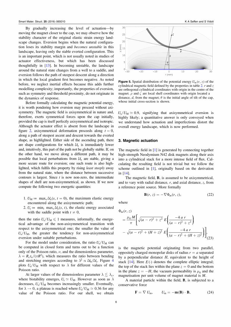
Figure 5. Spatial distribution of the potential energy ( )U r z,m of thecylindrical magnetic field defined by the properties in table 2. r and zare orthogonal cylindrical coordinates with origin in the centre of themagnet. r and z are local shell coordinates with origin located adistance, d, from the magnet; q is the initial angle of tilt of the cap,whose initial cross-section is shown.

6

Smart Mater. Struct. 25 (2016) 065010 K A Seffen and S Vidoli

where ( )m B is the magnetization induced by the magneticfield and Um is the potential energy associated with themagnetic field. It has been experimentally observed [15], thatthe magnetisation of a material particle of volume dV is wellfitted by the following linear relation

( ) ( )dcm

= Vm B B d , 250

where dc is a dimensionless number indicating the magneticsusceptibility of the material composing the shell [16]. Usingthis approximation, the potential energy of the magneticforces acting on every infinitesimal volume dV of shell is

( ) ( ) · ( ) ( )dcm

= -U r z r z r z VB B, , , d . 26m0

Equation (26) must be integrated over the volume ofshell, in order to obtain the total magnetic energy associatedwith the shell. We may use the original shell cylindricalcoordinates from section 2, resulting in r f r=V td d de .However, since we want the shell to move inside the refer-ence frame ( )r z, of the magnet, we introduce the followingchange of coordinates

≔ ( )≔ [ ( ) ] ( )**

r q z qz q r q+

+ -r s t

z h d s t

cos , sin ,

, cos sin , 27

where (·)h is the unit step function. Here, r* and z* indicatethe coordinates of a generic point of the shell; d is theproximity distance between the centre of the shell and theupper surface of the magnet; and q is the angular rotation ofthe z axis (attached to the shell) with respect to the z (attachedto the magnet), i.e. q is the tilt angle of the shell, see figure 5.Moreover, ( ) ˆ ( )z r f=s t w, ,ts, must be computed accordingto the ansatz equation (7), which will lead to an explicitdependance of the magnetic energy on the actual shell shape.The unit step function h is used when we want to avoidinterpenetration of the magnet and shell by ensuring * z 0.

Finally, we obtain the total potential energy of the shellas the following integral

( ) ( ) ( )* * ò òq r r f=p

s t d t U r z, ; , , d d . 28R

m e0 0

2

m

The energy functional, m, depends on the shell configurationthrough the parameters (s, t) and the relative position andorientation through d and θ. The function has to be evaluatednumerically: using a standard CPU Core at 2.8 GHz andWOLFRAM MATHEMATICA [17], 100 evaluations takes about15 s. The magnetic properties and geometry of the magnetused in [1] are given in the following table.

4. Total energy

The total energy of the actuated shell is the sum of elasticand magnetic energy components:

( ) ≔ ( ) ( ) ( ) q q+s t d s t s t d, ; , , , ; , . 29e m

Clearly, at large distances from the magnet ( ¥d ), themagnetic energy is negligible and reduces to the elasticstrain energy landscape in figure 2 with two stable equilibria:this is the ‘far-field’ case. When d is reduced, the magneticcontribution increases, and begins to differ from e, which,in turn, affects the stability of the original equilibria. By wayof example, we plot in figure 6 as a function of s only,stipulating t=0 and q = 0, for three values of d above theexperimental threshold of eversion: 1 m, 20 mm and 14 mm.For the largest d, the equilibria are unaltered see figure 3,whereas for =d 20 mm, the magnet is close enough to distortthe initial state, observed as a slight movement of the originalminimum along the s-axis. For the smallest d, the curvepassing through the original minimum is now noticeablymore rotated as this stationary point transforms into a point ofinflexion. All everted configurations are local minima andalways stable, and their locations along s increase beyond0.995, indicating that they become more distorted than thefar-field shape. Negative values of are justified since wechoose the initial configuration to have a vanishing energy inthe far-field case.

Figure 6. Energy performances for three distances of magnet fromthe cap; d=1 m, 20 mm and 14 mm: total energy, , (solid) andmagnetic energy, m, (dashed). Axisymmetry is imposed by settingq = 0 and t=0.

Figure 7. Total energy, , for d=7 mm and q = 0 . The orangepoints show a possible eversion path. Each point is a solution ofequation (31) over a fixed interval of time, which imposes artificialdamping in proportion to the local gradient.

7

Smart Mater. Struct. 25 (2016) 065010 K A Seffen and S Vidoli

If d is decreased further, the initial state becomes a pointof inflexion and unstable in the direction >s 0. The systemwill naturally move along the path of steepest descent towardsthe stable everted configuration. However, we also need toascertain the landscape elevation around this path when t isnon-zero in view of the propensity for non-axisymmetricaleversion. This is now considered for caps with and withoutinitial tilt angles.

5. Simulations

5.1. Vanishing tilt angles: axisymmetrical eversion

For vanishing tilt angles, q = 0, it can be shown that the totalenergy, , is symmetrical with respect to t=0, i.e.

( ) ( ) ( ) q q= = - =s t d s t d, , , 0 , , , 0 . 30

By definition, the corresponding landscape is symmetricalabout the t=0 axis, which heavily favours axisymmetricaleversion. We can test this hypothesis by setting d=7 mm sothat the magnet is closer than required for eversion. The totalenergy is plotted in figure 7, where the original minimum at( ) ( )=s t, 0, 0 is now a saddle and has lost its stability. Thesystem will move away from this towards the stable evertedminimum around s=1.25. Because of symmetry aboutt=0, the eversion path follows a decreasing ridge and thetransition is axisymmetrical.

The spacing between points on the path has been cal-culated by solving the auxiliary equation

{˙ } ( ) ( ) q= -s t s t d, , , , , 31

where ∇ is the gradient function with respect to s and t and anoverdot denotes differentiation with respect to time. Thisequation is a statement of damping in the direction of steepestdescent and is analogous to the artificial ‘numerical’ damping

Figure 8. Top left: the eversion path in figure 7 superposed onto the landscape of elastic strain energy, e. Top right: values of e from (a)plotted with respect to fixed time intervals see the finite element data from figure 1. Bottom: the resulting axisymmetrical shell configurationsduring eversion.

Figure 9. Total energy, , for d=13 mm and q = 5 . The bluepoints show a possible eversion path; the grey points indicate howthe path is altered when contact is enforced between the deformedshell and the magnet.

8

Smart Mater. Struct. 25 (2016) 065010 K A Seffen and S Vidoli

Figure 10. Top left: the eversion paths of figure 9 superposed onto the elastic strain energy landscape, e. Top right: values of e along thesame paths plotted with respect to fixed intervals of time, see figure 1. Bottom: the shell configurations of the grey eversion path, wherecontact takes place with the magnet.

Figure 11. Left: continuation of the natural stress-free equilibrium, ( ) ( )=s t, 0, 0 , as the distance d from the magnet is decreased for initialangles of tilt; q = 0 , 1 , 5 , and 10°. Right: critical distance dc as a function of θ: dots are discrete solutions and the line is a best fit.

Table 1.Geometry and material properties of the shell cap in figure 1.

Rc R te Y ν

17.32 mm 18 mm 1.5 mm 750 kPa 0.5

Table 2. Properties of the magnet in figure 1.

m0 M dc a H

p ´ -4 10 7 N A−1 ´1.03 106 A m−1 0.20 25 mm 12 mm

9

Smart Mater. Struct. 25 (2016) 065010 K A Seffen and S Vidoli

used in finite element analysis for achieving convergentsolutions: when there are rapid changes in values, damping ishigher and solution points are more finely resolved for thesake of accuracy. The equation above therefore provides away of comparing to the time-oriented finite element dataeven though our framework does not include other dynamiceffects; equation (31) is solved for fixed intervals of time sothat the spacing between points is directly proportional to themagnitude of the local gradient. After calculating the (s, t)coordinates of each point, we extract the correspondingvalues of the elastic strain energy, e, from the totallandscape, which is rendered in figure 8(a). These valuesare then plotted for each time interval in figure 8(b). Thisprofile, encouragingly, replicates the features present in thefinite element output of figure 1, in particular, the highlightedsecond minimum. Strictly speaking, we need to consider non-axisymmetrical eversion from our analysis, which isperformed in the next section; however, these preliminaryresults give confidence to our solution methodology in viewof more sophisticated multi-physics analysis software. Thecorresponding shapes of shell are also plotted in figure 8(c).

5.2. Non-vanishing tilt angles: non-axisymmetrical eversion

Symmetry conditions are not imposed upon the performanceof the total energy, , and the initial conditions specifyd=13 mm and q = 5 , as in [1]. The landscape of isplotted in figure 9 and, again, we solve equation (31) overfixed intervals of time. Again, the stability of the naturalminimum near ( ) ( )=s t, 0, 0 is lost, which becomes a saddle;however, it is skewed in the direction of positive t, and theeversion path being directed away from the s-axis is thereforeone of non-axisymmetrical shapes. When contact between thedeformed shell and magnet is enforced by the condition of* >z 0 in equation (27), this path bifurcates as shown andfollows a different eversion route. This diversion happensearly on because the shell is more deformed on one side andmakes contact well before full eversion. We see this also inthe experiment in figure 1. Note that we are not modelling thecontact forces, so the evaluation of the elastic strain energyafter contact has been made may not be entirely correct. Bothsets of path points are superposed onto the elastic strainenergy landscape in figure 10(a), in order to construct thetime-evolution profiles in figure 10(b). Again, the featurescompare well to the finite element output in figure 1. Thedeformed shapes for the contacting case are displayed infigure 10(c).

5.3. Critical values of the distance

We finally address the dependence of the eversion threshold,d, upon θ. We tackled this by performing a numerical con-tinuation of the natural equilibrium branch for several tiltangles, see for instance [18]. For any θ, this branch originatesfrom the point ( ) ( )=s t, 0, 0 as ¥d . The results areshown in figure 11 and can be summarised as follows.

• For a given angle of tilt, there exists a well defined criticalvalue of distance, denoted as ( )qdc , below which stabilityof the equilibrium branch is lost;

• the function ( )qdc for small tilt angles ∣ ∣ q 15monotonically increases from a minimum value of around7 mm for q = 0;

• a non-vanishing tilt angle ‘encourages’ eversion byenabling non-axisymmetrical shapes. This is evidentfrom figure 11(a), where the solution branches are plottedin the three-dimensional space ( )s t d, , : these arecharacterized by positive values of t well before theirstability is lost;

• a relevant sensitivity of the function ( )qdc is evident nearq = 0; one could expect the values d 11 mmc to berarely observed as any small imperfections in practicewould lead to a non-axisymmetrical eversion.

Thus, in a perfect world, the proximity distance foreversion is around 50% of the value of 13 mm observed inexperiments and in finite element analysis. This value quicklyrises as the tilt increases, reaching 13 mm when θ is just threedegrees. Thereafter, the rate of increase diminishes, so doesthe influence of the tilt angle, and eversion is non-axisymmetrical.

6. Conclusions

We have developed a two degree-of-freedom theoreticalmodel for predicting the general shapes of a linear elasticshell cap made of novel material, which ultimately evertsunder a magnetic field. We have advanced the general for-mulation for such problems by explicitly dividing the dis-placement field into axisymmetrical and antisymmetricalcomponents, so that we may explore the behaviour directlyunder both assumptions. We have included magnetic actua-tion for the first time in such a formulation, and we havefocussed on the total energy profile of the system, in order tounderstand its stability characteristics and how they changeduring actuation. Importantly, we have argued that becausewe have a closed system, actuation from the initial state willfollow the path of maximum descent from this position. Wehave been able to interrogate this graphically via the land-scapes we generate, for a more intuitive insight. We haveobtained good agreement with results from a leading study, inparticular, we have confirmed the proximity threshold foreversion, we have shown that an initial title angle is con-ducive for non-axisymmetrical eversion, and we have deter-mined that the critical threshold for eversion is stronglycontrolled by the tilt angle when the angle is small. Thegoodness of these qualitative comparisons give us confidenceabout our model’s overall robustness, which may then be usedto predict detailed information such as transverse displace-ments, materials stresses etc throughout the cap, and fur-thermore, to describe the performance of other shapes ofmagnetic shell. We therefore hope our approach may inspireothers to pursue modelling in this way in concert with com-putational studies.

10

Smart Mater. Struct. 25 (2016) 065010 K A Seffen and S Vidoli

Acknowledgments

The perspicacious comments of two anonymous reviewerswere gratefully received and implemented. Dr E G Loukaidesis thanked for earlier discussions with the authors.

Appendix

The coefficients ( )C s t,a k, in equation (18) for the expansionof the forcing term ( )-K Kdet det 0 can be easily computedto be for k=0 (namely the terms independent of f):

( )

( )

( )

( )

( ) ( )

= - +

=- + -

= - +

=- -

= +

C s ts

st

C s ts

R

s

R

t

R

C s ts

R

s

R

t

R

C s ts

R

t

R

C s ts

R

t

R

,25

45

72

289,

,75

4

15

2

324

289,

,1275

64

15

4

3627

2312,

,75

8

270

289,

,125

64

125

578, 32

0,0

2 2

2,0

2

2 2

2

2

4,0

2

4 4

2

4

6,0

2

6

2

6

8,0

2

8

2

8

for k=1 (namely the terms proportional to fcos ):

( ) ( )

( )

( ) ( )( )

= - = -

= -

=- =

C s tst t

C s tt

R

st

R

C s tst

R

t

R

C s tst

RC s t

st

R

,90

17

36

17, ,

135

34

1125

68,

,5075

272

35

17,

,2565

272, ,

275

13633

0,1 2,1 2 2

4,1 4 4

6,1 6 8,1 8

and for k=2 (namely the terms proportional to fcos 2 ):

( ) ( )

( )

( ) ( ) ( )

= = -

=

=- =

C s tt

C s tt

R

C s tt

R

C s tt

RC s t

t

R

,216

289, ,

648

289,

,6045

2312,

,405

289, ,

175

578. 34

0,2

2

2,2

2

2

4,2

2

4

6,2

2

6 8,2

2

8

References

[1] Loukaides E G, Smoukov S K and Seffen K A 2014 Magneticactuation and transition shapes of a bistable spherical capInt. J. Smart Nano Mater. 5 270–82

[2] Seffen K A 2007 Morphing bistable orthotropic ellipticalshallow shells Proc. R. Soc. A 463 67–83

[3] Vidoli S and Maurini C 2008 Tristability of thin orthotropicshells with uniform initial curvature Proc. R. Soc. A 4642949–66

[4] Vidoli S 2013 Discrete approximations of the Föppl–vonKármán shell model: from coarse to more refined models Int.J. Solids Struct. 50 1241–52

[5] Brodland G W and Cohen H 1987 Deflection and snapping ofspherical caps Int. J. Solids Struct. 23 1341–56

[6] Thompson J M T and Hunt G W 1973 A General Theory ofElastic Stability (New York: Wiley)

[7] Kalnins A 1961 Free nonsymmetric vibrations of shallowspherical shells Proc. 4th US National Congress of AppliedMechanics

[8] Mansfield E H 1989 The Bending and Stretching of Plates(Cambridge: Cambridge University Press)

[9] Olver F W J 1974 Asymptotics and Special Functions (NewYork: Academic)

[10] Quapp W and Heidrich D 1984 Analysis of the concept ofminimum energy path on the potential surface of chemicallyreacting systems Theor. Chim. Acta 66 245–60

[11] Fernandes A, Maurini C and Vidoli S 2010 Multiparameteractuation for shape control of bistable composite plates. Int.J. Solids Struct. 47 1449–58

[12] Coburn B H, Pirrera A, Weaver P M and Vidoli S 2013Tristability of an orthtropic doubly curved shell Compos.Struct. 96 446–54

[13] Loukaides E G 2013 Elementary morphing shells PhDDissertation University of Cambridge

[14] Blinder S M 2011 Magnetic field of a cylindrical bar magnetWolfram Demonstrations Project

[15] Schaller V, Kräling U, Rusu C, Peterson K, Wipenmyr J,Krozer A, Wahnström G, Sanz-Velasco A, Enoksson P andJohansson C 2008 Motion of nanometer sized magneticparticles in a magnetic field gradient J. Appl. Phys. 104093918

[16] Gorodkin S R, James R O and Kordonski W I 2009 Magneticproperties of carbonyl iron particles in magnetorheologicalfluids J. Phys.: Conf. Ser. 149 012051

[17] (Wolfram Research, Inc.) 2015Mathematica 10.2 (Champaign,Illinois: Wolfram Research, Inc.)

[18] Allgower E L and Georg K 1990 Numerical ContinuationMethods: An Introduction (Berlin: Springer)

11

Smart Mater. Struct. 25 (2016) 065010 K A Seffen and S Vidoli