“excess volatility” and the german stock market,...
TRANSCRIPT

“Excess Volatility” and the German Stock Market, 1876–
1990
J. Bradford De Long
Harvard University and NBER
Marco Becht
European University Institute
March 19921
Abstract
This paper uses long-run real price and dividends series to investigate for the Germanstock market the questions asked of the U.S. market by Shiller (1989). It tries todetermine in what periods and to what degree the German stock market has alsopossessed “excess volatility” in the past century. It finds no evidence of excessvolatility in the pre-World War I German stock market. By contrast, there is someevidence of excess volatility in the post-World War II German stock market. The roleplayed by the German Großbanken in the pre-World War I stock market might be thecause of the low comparative volatility of German stock indices before 1914.
JEL Classification Numbers C12, G14, G21, N23.
Keywords: Excess Volatility, Variance Bounds Tests, Efficient Markets Hypothesis,German Stock Market History, German Universal Banks (Großbanken)
I. Introduction
This paper examines “excess volatility” in the German stock market, investigating for that market
the issues examined by Robert Shiller (1981, 1986, 1989) for the U.S. stock market.2 It finds some
evidence that post-World War II German stock index prices have been too volatile (relative to naïve
1J. Bradford De Long is Danziger Associate Professor of Economics at Harvard University. Marco Becht is a Ph.D.candidate at the European University Institute. This research was partially supported by the National Science Foundation,by the NBER, and by the EUI. We would like to thank Robert Barsky, George Bulkley, Daniel Raff, Robert Shiller, PeterTemin, and Robert Waldmann for helpful discussions, and the Frankfurter Wertpapierbörse AG, the Commerzbank AG,the Siemens Museum Munich, the Library of the Frankfurter Industrie- und Handelskammer, the Statistisches Bundesamtand the Frankfurter Allgemeine Zeitung for helpful assistance with long-run stock price data.2The literature sparked by Shiller and by LeRoy and Porter (1981) has for the most part assumed that the real interest rateat which future dividends are discounted is a constant. This assumption is surely false: for example, the ex ante real rate ofdiscount for the U.S. stock market at the end of World War I was on the order of thirty percent per year for the first twoyears after the war in anticipation of the forthcoming postwar deflation. Thus it was much higher than the discount rateduring normal times. However, investigators have had little success accounting for stock price volatility via shifts in thereal riskless rate, or in the real spread between riskless and market rates of discount driven by changes in risk tolerance(see Shiller, 1989).

“Excess Volatility” and the German Stock Market 2 De Long and Becht
estimates of fundamentals) to have been rational forecasts of the present value of future dividends.
Alternatively, pre-World War I stock prices were not volatile enough (relative to naïve estimates of
fundamentals).3 In either case, the efficient markets hypothesis appears inconsistent with observed
behavior in one or the other of the periods.4 The focus of this paper is on the divergence of market
outcomes in the two periods, and the difficulty of reconciling both patterns simultaneously with the
efficient markets hypothesis.
This paper examines the volatility of prices relative to dividends in order to avoid most of the
biases in estimated volatility ratios generated by Shiller’s (1981) original tests. Thus normalized, the
pre-World War I German stock market shows not excess but deficient volatility: the market price-
dividend ratio is surprisingly far down in the lower tail of the distribution under the null hypothesis
that prices are rational forecasts of fundamentals. Throughout the pre-World War I era, the market
average dividend yield fluctuates in a narrow band between four and a half and five and a percent. By
contrast, the post-World War II stock market (and especially the post-Wirtschaftswunder market)
shows some evidence of “excess” volatility. The evidence of excess volatility in post-World War II
German data is weaker than but of the same order of magnitude as the evidence using U.S. post-
World War II data.
The behavior of the pre-World War I German stock market thus is in sharp contrast to the
behavior of the post-World War II German stock market, and to the behavior of the U.S. stock market
in either the pre-World War I or the post-World War II period. We speculate that the dominance of
the German Großbanken in the securities industry in the years before World War I may be the cause
of the exceptional behavior of the pre-World War I German market.
After this introduction, the second section of this paper describes the data used. The third section
explains the approach used and documents the divergence between the pre-World War I and the post-
World War II behavior of German stock market aggregates. The generating processes necessary to
reconcile the post-World War II behavior of German stock index prices with the efficient markets
hypothesis lead to the conclusion that the market’s small degree of volatility in the pre-World War I
era is anomalous. Generating processes that fit the market’s low pre-World War I volatility lead to the
3Understood to also include the ancillary assumption of a constant real discount rate.4Little can be said about the relative excess volatility of the German stock market over 1914–50; there are too many “pesoproblems” present for any analysis to be convincing; see Eichengreen (1991).

“Excess Volatility” and the German Stock Market 3 De Long and Becht
conclusion that the post-World War II market exhibits excess volatility. Unless the specification of
the dividend process is itself a free variable that shifts substantially from World War I to post-World
War II reconstruction, it is very difficult to reconcile both periods with the dividend discount model.
Section IV provides a brief summary of the argument. Appendices discuss the choices made in
constructing the data, and the statistical significance of some of the results obtained.
II. German Data
Donner (1934) compiles and reports a monthly nominal share price index—with attached
estimates of average yearly dividend yields for the companies included in his aggregate index—for
the German stock market from January 1870 to December 1913. His index covers only twelve
companies from 1870 to 1875.5 The number of companies covered reaches twenty-one in 1876 and is
nearly sixty by 1890. The original twelve companies covered in 1870 include four banks, four
railroads, and four mining companies.6 Railroads disappear from the index with their nationalization
in 1890. Companies in other industries are added as industrialization proceeds.7
Especially in the years from 1890 on, the Donner index is a sample of Germany’s largest
companies, weighted toward those heavy industries in which Germany’s companies were largest and
its international comparative advantage greatest. We begin our study in 1876, when the number of
companies in the index rises above twenty.
Donner’s index ends with the beginning of World War I. An official index—unfortunately
without dividends attached—covers the period from 1914 up to the 1923–24 hyperinflation
(Statistisches Reichsamt, 1922a, 1922b). A second official index covering three hundred corporations
extends from 1924 to the middle of World War II, reporting both the stock index price and a dividend
yield (Statistisches Reichsamt, 1928, 1929). We splice the first official Statistisches Reichsamt
(National Bureau of Statistics) series onto Donner’s in 1914 to track the course of the German stock
5Earlier indices covering the 1856–70 period are also available from Däbritz (1929). Unfortunately, they too are based ona very small sample of securities.6Two mining companies—the Bochumer Verein für Bergbau and Gußstahlfabrik and the Hoerder Bergwerks- undHüttenverein—also had metal fabrication or railway divisions.7On the eve of World War I, the index covers eight banks, two shipping companies, fourteen mining and steel producers,four electrical machinery manufacturers, four utilities, nine metalworking manufacturers, six in chemicals, seven intextiles, two in paper and wood products, three makers of building materials, two construction companies, three glass andporcelein manufacturers, and four breweries.

“Excess Volatility” and the German Stock Market 4 De Long and Becht
market up to the hyperinflation. We splice the second Reichsamt index onto the first to provide
information about the course of the German stock market between the hyperinflation and the middle
of World War II.
For the post-World War II period, the stock price series we use links four official portfolio index
series constructed by the post-World War II Statistisches Bundesamt (Federal Bureau of Statistics).
We link from each series to the next in the first year in which the following sequence becomes
available (see Herrman, 1956; Spellerberg and Schneider, 1967; Silberman, 1974; Lützel and Jung,
1984; Statistisches Bundesamt, 1985).
For the later interwar and the post-World War II periods, the yield series used is the yield on all
traded stocks. Thus the yield is calculated from a different and larger sample of corporations than are
the price indices. Nevertheless, the post-World War II dividend series—calculated by multiplying
price and yield—is a good estimate of the dividend corresponding to the index.8
The nominal price and dividend series are deflated by the German consumer price index endorsed
by the Deutsche Bundesbank (1976). This index runs continuously, with one gap covering World War
II and the post-war reconstruction period.9
Appendix 1 presents the various alternative stock price and dividend yield series available for the
German market. Its table A.1 reports the underlying real stock price, yield, and consumer price index
series used here. In all cases we use annual average prices and annual average dividend yields. The
ways in which earlier authors report their results make annual average data more readily available
than point-in-time data. Moreover, markets for many of the securities in the indices are thin.
Transitory episodes of market disruption—like the liquidity crunch that followed the bankruptcy of
the Austrian Creditanstalt during the Great Depression—are not uncommon. With point in time data,
such events could introduce noise into a market that may be exhibiting relatively good performance
8The post-World War II price index series covers close to ninety-five percent of the par value of stocks traded on theGerman exchanges.9It was assembled from four different sources. Up until 1914 the cost of living figures come from Kuczynski (1947), whoinvestigated the standard of living of Geman workers since 1800. Kuczynski’s cost of living index consists of estimates offood prices and housing costs. From 1915 to 1919 the index is derived from calculations by the Statistisches Bundesamt,the Federal Statistical Bureau of post-World War II West Germany, made after World War II in order to close the gapbetween Kuczynski’s and the subsequent indices. From 1920 to 1940 the cost of living index is that compiled for a five-person working-class household by the Statistisches Reichsamt , the National Statistical Bureau of first the WeimarRepublic and then the Third Reich. For the post-World War II years from 1949 to the present, the cost of living index usedis that calculated for a four-person middle-class household by the Statistisches Bundesamt (1990). The different consumerprice series have different base years. They chart the changes in the price level for different consumption bundles, and arenot completely consistent. The Deutsche Bundesbank (1976) reports similar indices for wholesale prices, and a lesscomplete national product deflator.
“Excess Volatility” and the German Stock Market 5 De Long and Becht
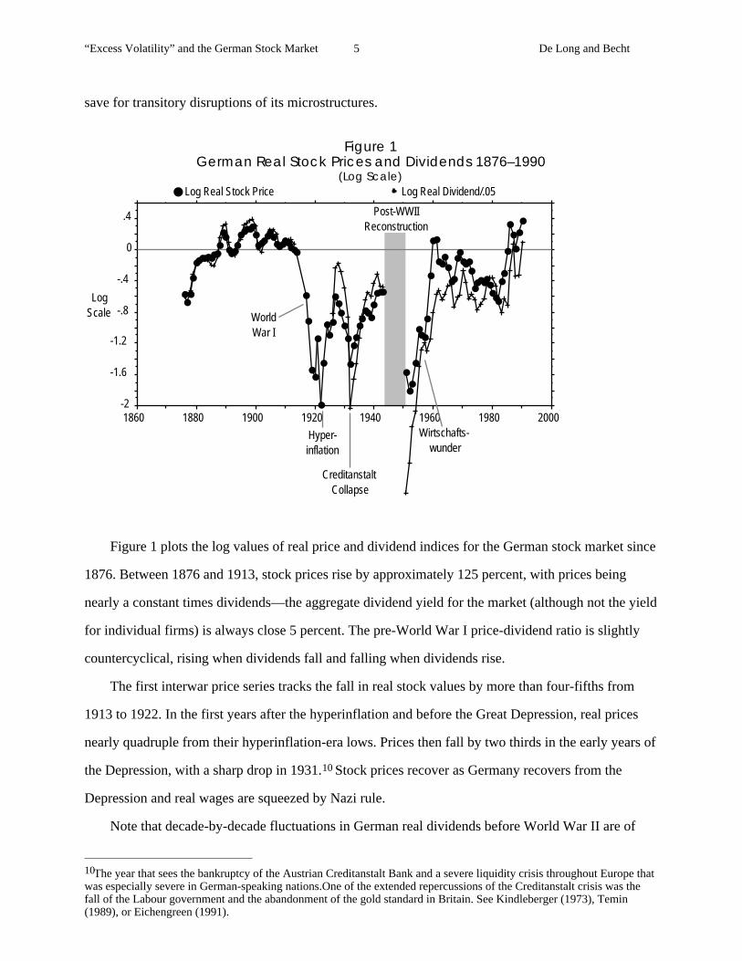
save for transitory disruptions of its microstructures.
Figure 1German Real Stock Prices and Dividends 1876–1990
(Log Scale)
-2
-1.6
-1.2
-.8
-.4
0
.4
1860 1880 1900 1920 1940 1960 1980 2000
Log Real Stock Price Log Real Dividend/.05
Log
Scale World
War I
Hyper-
inflation
Creditanstalt
Collapse
Post-WWII
Reconstruction
Wirtschafts-
wunder
Figure 1 plots the log values of real price and dividend indices for the German stock market since
1876. Between 1876 and 1913, stock prices rise by approximately 125 percent, with prices being
nearly a constant times dividends—the aggregate dividend yield for the market (although not the yield
for individual firms) is always close 5 percent. The pre-World War I price-dividend ratio is slightly
countercyclical, rising when dividends fall and falling when dividends rise.
The first interwar price series tracks the fall in real stock values by more than four-fifths from
1913 to 1922. In the first years after the hyperinflation and before the Great Depression, real prices
nearly quadruple from their hyperinflation-era lows. Prices then fall by two thirds in the early years of
the Depression, with a sharp drop in 1931.10 Stock prices recover as Germany recovers from the
Depression and real wages are squeezed by Nazi rule.
Note that decade-by-decade fluctuations in German real dividends before World War II are of
10The year that sees the bankruptcy of the Austrian Creditanstalt Bank and a severe liquidity crisis throughout Europe thatwas especially severe in German-speaking nations.One of the extended repercussions of the Creditanstalt crisis was thefall of the Labour government and the abandonment of the gold standard in Britain. See Kindleberger (1973), Temin(1989), or Eichengreen (1991).

“Excess Volatility” and the German Stock Market 6 De Long and Becht
larger proportional magnitudes than decade-by-decade fluctuations in real price indices. In this
respect the pre-World War II German stock market is different from the United States, where decade-
by-decade price fluctuations are proportionally larger than dividend fluctuations (see Barsky and De
Long, 1989 and 1990).
Post-World War II data begin in 1951. Throughout the 1950’s real prices and dividends rise very
rapidly—by a factor of eight—with the price-dividend ratio reaching a high near fifty in 1960. Since
1960 the index has recorded relatively slow growth in real prices and dividends. Even so, price
changes have been substantial: the real stock index falls by nearly half between 1960 and 1966. It
more than doubles over the short four year period between 1981 and 1985.
From 1960 on, fluctuations in prices have been proportionately larger than fluctuations in
dividends. Over 1960–66, the log of real stock prices falls by 0.55 while log real dividends fall by
only 0.2; over 1966–72, log prices rise by 0.3 while log dividends rise by 0.2; over 1972–82, log
prices fall once again by 0.55 while log dividends fall by only 0.15; and over 1982–1990 log prices
rise by 1.1 while log dividends rise by 0.8. This post-Wirtschaftswunder pattern, in which swings in
dividend levels are paced by more than proportional swings in prices, is reminiscent of the behavior
of the U.S. stock market, as analyzed by Barsky and De Long (1989). It suggests that investors value
the market by extrapolating recent dividend changes into the future.
The real stock price series constructed here has a gap covering the second half of World War II
and the postwar reconstruction period from 1943–1950. We have been unable to recover sufficient
data on dividend yields and price indices to link the series across this period. The real price indices
are not comparable across the break at the end of World War II.11
The real dividend series has two breaks. One covers World War I and the interwar period up to
the hyperinflation. The second covers the end of World War II and the postwar reconstruction period.
Thus we do not have enough data to conduct Shiller-like analyses of the era from the beginning of
World War I to the beginning of the 1950’s.
This paper analyzes the pre-World War I and the post-World War II periods separately. For the 11The failure of the German stock market to fall in real terms during the war or during the approach to war is somewhatsurprising. To some degree, wartime prices are false prices. Although trading on the Frankfurt exchange continues untilthree days before the arrival of the American army, prices on the exchange are frozen in March 1943. Foreign quotationson the market had been prohibited as early as 1937. And dividends had been regulated from early in the National Socialistera. After December 1934 dividend payments to shareholders could not exceed six percent. Any excess was paid into a“Patriotic Fund.” Although credited to shareholders’ accounts with the “Patriotic Fund,” such forced loans were notliquid—and of course were never repaid.
“Excess Volatility” and the German Stock Market 7 De Long and Becht
pre-World War I period, it takes 1913 as its terminal condition: the level of real stock prices in 1913 is
a proxy for the rational expectation, on the eve of the unexpected coming of World War I, of the
fundamental value of German securities. The level of stock prices in 1990 stands in for the rational
expectation of the expected value of German securities today.
III. Excess Volatility and the German Stock Market
Shiller’s (1981, 1989) first key insight was that the level of the stock market is a forecast of the
ex post perfect-foresight fundamental. An investor who buys and holds, and pays less than the ex post
fundamental, receives a supernormal return. Arbitrage, therefore, pushes prices in an efficient market
to be efficient forecasts of the perfect-foresight fundamental.
Shiller’s second key insight was to apply the principal that efficient forecasts are less volatile
than the ex post realized values of the quantities being forecast. If a forecast is more volatile, a better
forecast could be constructed easily: shrink the original forecast toward its ex ante unconditional
mean, and the resulting improved forecast will have a smaller mean squared error. These two insights
imply that if the efficient markets hypothesis holds then stock prices should be less volatile—relative
to their ex ante unconditional means, a notion that needs to be made precise—than the realized track
of the ex post perfect-foresight fundamental.
Biases in Testing for Excess Volatility
As Flavin (1985), Scott (1985), Kleidon (1986a and 1986b), Mankiw, Romer, and Shapiro (1985,
1991), and many others have argued, Shiller’s (1981) original comparison of the variance of
detrended prices and of detrended ex post perfect-foresight fundamentals is subject to biases.
Especially in small samples, such tests may well find apparent excess volatility even if in fact the
efficient markets hypothesis holds.
It is easiest to understand the source of these biases by examining the trading strategies
associated with tests of excess volatility and return predictability. Each test of market rationality is
implicitly associated with a portfolio strategy. If prices are too volatile relative to trend, investors at
the time could have made better forecasts of ex post fundamentals—and earned high profits—by
“Excess Volatility” and the German Stock Market 8 De Long and Becht
taking as their forecast some linear combination of the market price and a time trend, and betting that
returns would be low whenever the market price was above the trend. If returns are predictable from a
variable like the price-dividend ratio (Scott, 1985), investors could have earned supernormal profits
by buying when the ratio was low and selling when it was high.
If investors could in fact have followed the trading strategy implicit in the tests of market
efficiency—and did not—then the rejection of market efficiency is genuine. But under some
conditions the implicit trading strategy could not have been followed because it required more
information for its execution than investors at the time possessed. In such a case, the rejection of
market efficiency may well be spurious: investors may well have taken advantage of all profit
opportunities open to them, and given the information at their disposal prices may have been the best
available forecasts of the present value of fundamentals.
For example, suppose log dividends follow a random walk with drift:
(1) dt
= dt-1
+ g + εt
Where g is the long-run upward rate of drift of dividends, and εt is an innovation, unforecastable
before period t. With a constant discount rate r, the efficient markets log real stock price will be:
(2) pt
= -ln(r-g) + dt
Suppose an ex post time trend π is fitted to the first and last observations, t=0 and t=T:
(3) πt
= p0
+Tt(p
T
- p0
)
Calculate the covariance between the one-year realized return r*t1:
(4) r*t
1= r + ε
t
and the price relative to the ex post time trend (conditional on knowledge of the current price pt and of
the current value πt of the ex post trend):
(5) E{r*t
1(p
t-π
t) | p
t-π
t} = -{Tt}E{ε
t+12 | p
t-π
t}Equation (5) shows that there are excess returns from buying when the price is low relative to the ex
post trend, and selling when it is high. Such a strategy eans excess returns off of the correlation
between the deviation of the price from the ex post trend and future innovations.
Why don’t rational investors take advantage of this correlation? Because at the time they must
“Excess Volatility” and the German Stock Market 9 De Long and Becht
trade they do not yet know what the end-of-sample value πT will be, and so cannot calculate the
current value of the ex post time trend πt. Investors would love to know πT—such knowledge would
allow them to calculate the value of the sum of the ε innovations yet to come. But they do not.
The return predictability in equation (5) comes solely from the use of the realized values of future
shocks—shocks dated later than t—in constructing the value πt of the time trend, and in assessing
whether prices are relatively low or high. Without this use of information about the realizations of
future shocks, there are no excess returns to be earned: returns are uncorrelated with the deviation of
the price from an ex ante time trend π’t constructed by extrapolating drift from the series starting
point.
(6) π't= p
0 + tg
(7) E{r*t
1(p
t-π'
t)| p
t, π'
t} = 0
In this example, a regression of returns on prices and an ex post time trend is indeed likely to find
significant return predictability and excess volatility. But such a finding is spurious: it arises from an
implicit assumption that rational investors had more information about future shocks than they in fact
possessed future shocks.
Normalizing by the Level of Dividends
To compensate for such biases, Mankiw, Romer, and Shapiro (1985 and 1991) proposed an
alternative benchmark for the calculation of excess volatility. They argued that it is plausible that past
investors knew naïve forecasts of perfect-foresight fundamentals made by assuming them to be a
constant dividend multiple. Tests of excess volatility relative to this alternative naïve-forecast
benchmark that takes fundamentals to be a constant multiple of dividends assume less in terms of
investors’ knowledge of the parameters and outcomes of the dividend process.
This paper uses such a naïve constant dividend multiple forecast as the benchmark against which
to evaluate the efficient markets hypothesis.12 It normalizes real prices and ex post fundamentals by
the current level of dividends. Figure 2 plots real prices and ex post fundamentals normalized by a
12Note, however, that it is possible to imagine situations—especially in circumstances of rapid development and uncertainlong-run growth paths—in which even the assumption that investors know ex ante of the average price/dividend ratio isincorrect, and in fact attributes to past investors information that they do not but would dearly wish to know. See Barskyand De Long (1989).

“Excess Volatility” and the German Stock Market 10 De Long and Becht
constant—twenty—multiple of dividends, for a real discount rate of 8 percent chosen to match real
returns over the century as a whole.
In figure 2 the pre-World War I stock market does not appear excessively volatile to the eye: the
volatility of prices relative to the benchmark of twenty times dividends is smaller than the volatility of
ex post fundamentals. The post-World War II market does see a larger volatility for prices relative to
the twenty times dividends benchmark than for ex post fundamentals after 1960. The decade before
1960 sees both prices and ex post fundamentals very far from normal multiples of dividends.
-.4
0
.4
.8
1880 1900 1920 1940 1960 1980
Prices Ex Post Fundamentals
Log
Scale
Figure 2
Prices and Ex Post Fundamentals Normalized by Twenty Times
Dividends
Pre-World War I and Post-World War II Prices, and Perfect-Foresight Fundamentals
Figures 3 and 4 provide individual looks at the behavior of prices, dividends, and perfect-
foresight fundamentals in the pre-World War I and post-World War II periods. They plot for each of
these periods the log levels of prices, the log ex post perfect-foresight fundamental (calculated using
an eight percent per year real discount rate), and also the log level of dividends (multiplied by twenty
in order to place it on the same scale as the other two series).
Note the wider variability of stock prices in the post-World War II period that leads figure 4 to
“Excess Volatility” and the German Stock Market 11 De Long and Becht
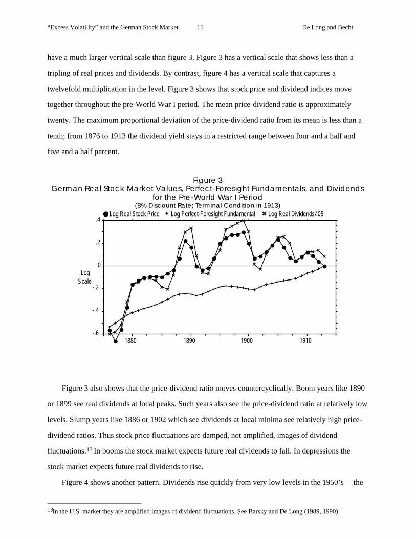
have a much larger vertical scale than figure 3. Figure 3 has a vertical scale that shows less than a
tripling of real prices and dividends. By contrast, figure 4 has a vertical scale that captures a
twelvefold multiplication in the level. Figure 3 shows that stock price and dividend indices move
together throughout the pre-World War I period. The mean price-dividend ratio is approximately
twenty. The maximum proportional deviation of the price-dividend ratio from its mean is less than a
tenth; from 1876 to 1913 the dividend yield stays in a restricted range between four and a half and
five and a half percent.
Figure 3German Real Stock Market Values, Perfect-Foresight Fundamentals, and Dividends
for the Pre-World War I Period(8% Discount Rate; Terminal Condition in 1913)
-.6
-.4
-.2
0
.2
.4
1880 1890 1900 1910
Log Real Stock Price Log Perfect-Foresight Fundamental Log Real Dividends/.05
Log
Scale
Figure 3 also shows that the price-dividend ratio moves countercyclically. Boom years like 1890
or 1899 see real dividends at local peaks. Such years also see the price-dividend ratio at relatively low
levels. Slump years like 1886 or 1902 which see dividends at local minima see relatively high price-
dividend ratios. Thus stock price fluctuations are damped, not amplified, images of dividend
fluctuations.13 In booms the stock market expects future real dividends to fall. In depressions the
stock market expects future real dividends to rise.
Figure 4 shows another pattern. Dividends rise quickly from very low levels in the 1950’s —the
13In the U.S. market they are amplified images of dividend fluctuations. See Barsky and De Long (1989, 1990).

“Excess Volatility” and the German Stock Market 12 De Long and Becht
period of the “economic miracle.” In 1955 real dividends are five times their 1951 level. In 1960 real
dividends are eighty percent above their 1955 levels. Real prices rise rapidly from 1951 to 1960,
rising by a cumulative factor of more than eight over the decade. The price-dividend ratio is almost
one hundred at the beginning of the 1950’s as firms skimp on payouts to increase capital available for
reinvestment. The price-dividend ratio falls until 1957, reaching a value in the low twenties. It then
rises and reaches another peak, near fifty, at the end of the 1950’s.
Figure 4German Real Stock Market Value, Perfect-Foresight Fundamentals, and Dividends for
the Post-World War II Period(8% Discount Rate; Terminal Condition in 1990)
-2
-1.6
-1.2
-.8
-.4
0
.4
1950 1960 1970 1980 1990
Log Real Stock Price Log Perfect-Foresight Fundamental Log Real Dividends/.05
Log
Scale
Since 1960 and the end of the Wirtschaftswunder, the real value of the German stock market
index has risen by relatively little. Real values in 1989 were only some twenty-five percent above
their 1960 levels. By contrast, real dividends have doubled over their 1960 levels. This stagnation in
the level of the market over the past generation has been accompanied by substantial short-run swings
in the real index price. Of these, the largest in magnitude is the four-year bull market from 1981 to
1985. It saw real prices nearly triple.
“Excess Volatility” and the German Stock Market 13 De Long and Becht
Volatility Ratios
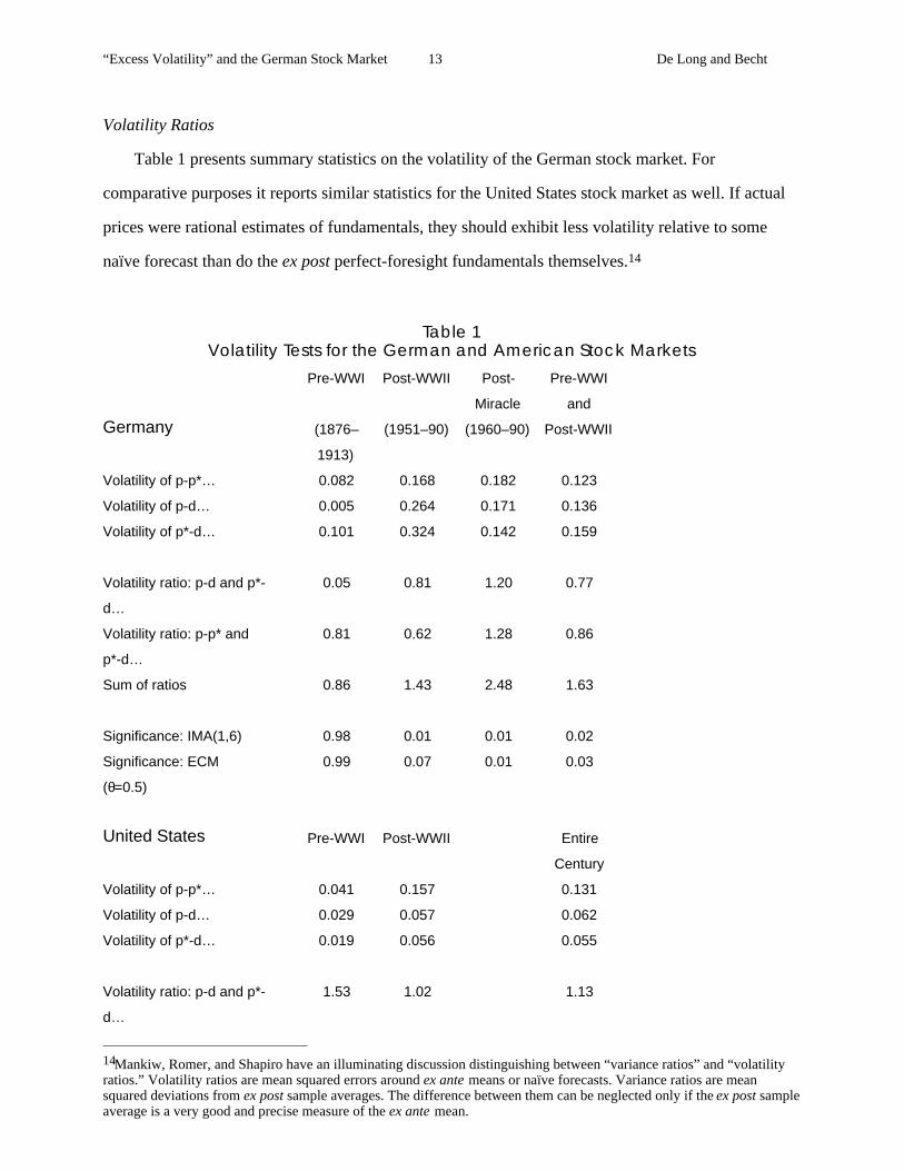
Table 1 presents summary statistics on the volatility of the German stock market. For
comparative purposes it reports similar statistics for the United States stock market as well. If actual
prices were rational estimates of fundamentals, they should exhibit less volatility relative to some
naïve forecast than do the ex post perfect-foresight fundamentals themselves.14
Table 1Volatility Tests for the German and American Stock Markets
Pre-WWI Post-WWII Post-
Miracle
Pre-WWI
and
Germany (1876–
1913)
(1951–90) (1960–90) Post-WWII
Volatility of p-p*… 0.082 0.168 0.182 0.123
Volatility of p-d… 0.005 0.264 0.171 0.136
Volatility of p*-d… 0.101 0.324 0.142 0.159
Volatility ratio: p-d and p*-
d…
0.05 0.81 1.20 0.77
Volatility ratio: p-p* and
p*-d…
0.81 0.62 1.28 0.86
Sum of ratios 0.86 1.43 2.48 1.63
Significance: IMA(1,6) 0.98 0.01 0.01 0.02
Significance: ECM
(θ=0.5)
0.99 0.07 0.01 0.03
United States Pre-WWI Post-WWII Entire
Century
Volatility of p-p*… 0.041 0.157 0.131
Volatility of p-d… 0.029 0.057 0.062
Volatility of p*-d… 0.019 0.056 0.055
Volatility ratio: p-d and p*-
d…
1.53 1.02 1.13
14Mankiw, Romer, and Shapiro have an illuminating discussion distinguishing between “variance ratios” and “volatilityratios.” Volatility ratios are mean squared errors around ex ante means or naïve forecasts. Variance ratios are meansquared deviations from ex post sample averages. The difference between them can be neglected only if the ex post sampleaverage is a very good and precise measure of the ex ante mean.
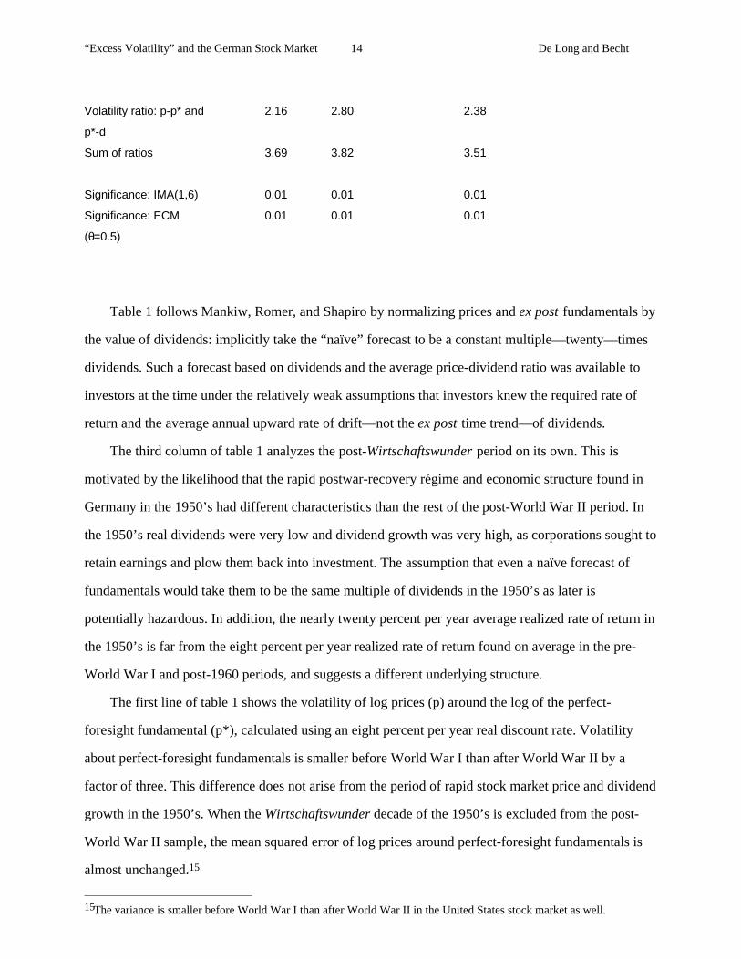
“Excess Volatility” and the German Stock Market 14 De Long and Becht
Volatility ratio: p-p* and
p*-d
2.16 2.80 2.38
Sum of ratios 3.69 3.82 3.51
Significance: IMA(1,6) 0.01 0.01 0.01
Significance: ECM
(θ=0.5)
0.01 0.01 0.01
Table 1 follows Mankiw, Romer, and Shapiro by normalizing prices and ex post fundamentals by
the value of dividends: implicitly take the “naïve” forecast to be a constant multiple—twenty—times
dividends. Such a forecast based on dividends and the average price-dividend ratio was available to
investors at the time under the relatively weak assumptions that investors knew the required rate of
return and the average annual upward rate of drift—not the ex post time trend—of dividends.
The third column of table 1 analyzes the post-Wirtschaftswunder period on its own. This is
motivated by the likelihood that the rapid postwar-recovery régime and economic structure found in
Germany in the 1950’s had different characteristics than the rest of the post-World War II period. In
the 1950’s real dividends were very low and dividend growth was very high, as corporations sought to
retain earnings and plow them back into investment. The assumption that even a naïve forecast of
fundamentals would take them to be the same multiple of dividends in the 1950’s as later is
potentially hazardous. In addition, the nearly twenty percent per year average realized rate of return in
the 1950’s is far from the eight percent per year realized rate of return found on average in the pre-
World War I and post-1960 periods, and suggests a different underlying structure.
The first line of table 1 shows the volatility of log prices (p) around the log of the perfect-
foresight fundamental (p*), calculated using an eight percent per year real discount rate. Volatility
about perfect-foresight fundamentals is smaller before World War I than after World War II by a
factor of three. This difference does not arise from the period of rapid stock market price and dividend
growth in the 1950’s. When the Wirtschaftswunder decade of the 1950’s is excluded from the post-
World War II sample, the mean squared error of log prices around perfect-foresight fundamentals is
almost unchanged.15
15The variance is smaller before World War I than after World War II in the United States stock market as well.

“Excess Volatility” and the German Stock Market 15 De Long and Becht
The second line shows the volatility of the log price-dividend ratio (p - d) around a fixed constant
of twenty, the average ex post price-dividend ratio for the pre-World War I period. The second line
thus calculates the volatility of prices about the “naïve” forecast that would have been made by an
investor who knew the mean trend drift of dividends and the required rate of return over the pre-
World War I period, and nothing more. The price-dividend ratio shows almost no volatility in the pre-
World War I period, and considerable volatility in the post-World War II period. The third line of
table 1 shows the volatility of the log ex post perfect-foresight fundamental to dividend ratio (p* - d),
about the same constant of twenty.
If prices are more volatile relative to “naïve” forecasts than perfect-foresight fundamentals,
investors could and should have constructed a better forecast: a weighted average of the market price
and the naïve forecast would have generated smaller forecast errors. Thus the second line of the table,
the volatility of the price-dividend ratio, should under the efficient markets hypothesis be smaller than
the third line, the volatility of ex post perfect-foresight fundamentals about the naïve constant
dividend multiple forecast. Line four reports this volatility ratio.
Line five in table 1 calculates another volatility ratio. The volatility of the perfect-foresight
fundamental about the actual price should be less than the volatility of the perfect-foresight
fundamental about the naïve forecast. If this is not so, the actual price is a worse estimate of
fundamentals than the naïve forecast.
A final implication of the efficient markets hypothesis is that the two ratios of lines four and
five—the sum reported in line six—should add up to one. If not, the log difference between the price
and the perfect-foresight fundamental (p - p*) is correlated with the log price-dividend ratio (p - d).
Profits could have been earned by trading on this correlation of the price-dividend ratio and value
relative to price. Lines seven and eight report monte carlo estimated significance levels for tests of the
efficient markets hypothesis using the volatility ratio in line 6, assuming that log dividends follow
either an IMA(1, 6) or an error correction model. These monte carlo significance levels are discussed
at greater length below.
The bottom panel of table 1 reports analogous statistics for the United States stock market, for
analogous periods.
Much of the excess volatility literature over the past decade has been concerned with the finite-
“Excess Volatility” and the German Stock Market 16 De Long and Becht
sample distributions of volatility ratios like those in table 1. Advocates of the efficient markets
hypothesis have argued that high volatility ratios are not strong evidence against it because test
statistics have large tails under the efficient-markets null.
Believers in the efficient markets hypothesis have no need to resort to such defensive arguments
in the case of pre-World War I Germany. Both the volatility ratios in lines four and five are less than
one. The volatility ratios in lines 4 and 5 for the pre-World War I period are smaller than on average
under the null. Prices are not too volatile relative to dividends, they are insufficiently volatile. Prices
are much less volatile than perfect-foresight fundamentals relative to the naïve forecast. The market
price is a better estimate of the perfect-foresight fundamental than is the naïve constant dividend
multiple forecast. Thus tests based on market volatility ratios show no traces at all of excess volatility
in the German stock market before World War I.
The post-World War II German stock market does show volatility ratios in line 6 of table 1
greater than one, and thus might provide some evidence of excess volatility. Table 1 also reports
monte carlo estimates of the finite-sample statistical significance of the volatility ratios reported in
line 6. Significance levels are calculated for two sets of assumptions about the true process generating
dividends: first, that the log level of dividends follows an IMA(1, 6) with coefficients known to
investors; second, that the log level of dividends follows an error-correction model—in which each
year brings a shock to the fundamental value of the market, and the market’s dividend level adjusts to
close half of the gap between last year’s dividend and the current sustainable dividend/price ratio—set
out in appendix 2.
The IMA(1, 6) process was chosen because its integrated component allows shocks to the level of
dividends to persist permanently, yet its inclusion of six moving-average coefficients provides the
monte carlo dividend process with sufficient flexibility to closely match the actual short-run dividend
impulse response function. The error correction process (with its adjustment parameter θ=0.5) was
chosen because it was the process used by Mankiw, Romer, and Shapiro (1991), because it was used
by Merton and Marsh (1986) in their critique of Shiller, and because it can, with sufficiently slow
adjustment, generate very persistent shifts in rates of dividend growth close to those postulated by
Barsky and De Long’s (1989) interpretation of U.S. long-run stock market fluctuations.
The post-World War II period considered as a whole generates volatility ratios that are significant
“Excess Volatility” and the German Stock Market 17 De Long and Becht
rejections of the null hypothesis on the high side for the two generating processes considered.16
There is a strong argument that the post-World War II Wirtschaftswunder decade of the 1950’s
sees the German stock market following a different stochastic process than the later years of slower
growth. When the post-Wirtschaftswunder 1960–90 period is considered in isolation, its volatility
ratios are high enough to be very significant rejections of the null hypothesis.
As appendix 2 shows, the distributions of these test statistics are sensitively dependent on the
assumed parameters of the generating process. Sufficient smoothness in the dividend level and
instability in dividend growth, for example, can lead to high estimated volatility ratios even if the null
efficient markets hypothesis holds. But shifting to a dividend generating process that possesses larger
and more persistent changes in dividend growth does not make German data fit the efficient markets
hypothesis more closely: the pre-World War I era would then exhibit deficient, not excess volatility.
There are surely dividend process that have a high probability of generating volatility ratios as
large as those observed for the post-Wirtschaftswunder period. But for such a process, volatility ratios
as low as those observed for the pre-World War I era are extraordinarily unlikely. Similarly, assuming
a dividend process that generates volatility ratios as low as the values observed for the pre-World War
I era would magnify the significance of the excess volatility of the post-Wirtschaftswunder era. Only
under the assumption of a major shift from a dividend process nearly a random walk before World
War I to a process with substantial dividend smoothing after World War II would there be any
possibility of using the efficient markets hypothesis to account for the behavior in both periods—and
there is no sign in dividend autocorrelations of such a major shift in the dividend process between the
pre-World War I period and the post-1960 period.
An Alternative Benchmark
The conclusions reached using the constant dividend multiple benchmark are not fragile. They do
not depend sensitively on the choice of this particular naïve forecast benchmark against which to 16Appendix 2 considers additional generating processes. Nevertheless, the post-World War II era continues to show signsof excess volatility for all proposed generating processes save the error correction models with high values of θ. When θ isnear one, year-to-year dividend level changes are small and shifts in dividend growth rates are persistent. Accordingly, thevariability of the price-dividend ratio is large: a value of θ=0.8 implies that each year dividends adjust only one-fifth of theway to the “permanent” sustainable dividend level. This is a greater degree of relative smoothness in real dividends vis-a-vis prices than is in fact found in the sample. A value of θ=0.1 implies that each year dividends adjust ninety percent ofthe way to the “permanent” dividend level: this makes the price-dividend ratio too close to a constant to be consistent withthe data. Appendix 2 also plots sample price and dividend series for various values of θ from monte carlo simulations ofsignificance levels.

“Excess Volatility” and the German Stock Market 18 De Long and Becht
assess volatility. Shiller (1990) argues that the use of a constant multiple of a long moving average of
dividends as a naïve forecast benchmark is preferable to the use of current dividends. In the U.S.
dividends appear to have a substantial short-run mean-reverting component, and a long moving
average of lagged dividends is a lower variance estimate of ex post fundamental values. Shiller (1990)
finds stronger violations of volatility bounds using such a smoothed naïve forecast benchmark.
Table 2 presents volatility ratios using a ten-year moving average of lagged dividends as a
benchmark. The substantive conclusions are unchanged: the post-World War II era shows some
evidence of excess volatility, while the pre-World War I era shows no such evidence. Using the
Shiller (1990) benchmark pre-World War I era German stock market indices no longer appear
insufficiently volatile to be efficient market estimates of fundamentals, but the volatility ratios for the
pre-World War I period are close to the center of the distributions calculated in the monte carlo
simulations. As noted above, calculated significance levels should be regarded with suspicion, and
used gingerly. Nevertheless, the sharp difference in the characteristics of the pre-World War I and the
post-Wirtschaftswunder markets remains.
Table 2Volatility Tests for the German Market Using a Moving Average of Lagged Dividends
as the Naïve Forecast Benchmark
p0 a 10-Year Moving
Average of DividendsPre-WWI
(1876–
1913)
Post-WWII
(1951–90)
Post-
Miracle
(1960–
1990)
Volatility of p-p*… 0.082 0.164 0.176
Volatility of p-p0… 0.023 0.316 0.204
Volatility of p*-p0… 0.090 0.338 0.109
Volatility ratio: p-p0 and
p*-p0…
0.26 0.93 1.86
Volatility ratio: p-p* and
p*-p0…
0.91 0.49 1.59
Sum of ratios 1.17 1.42 3.45
Significance: IMA(1,6) 0.27 0.06 0.01
Significance: ECM
(θ=0.5)
0.38 0.08 0.01

“Excess Volatility” and the German Stock Market 19 De Long and Becht
Still other naïve forecast benchmarks could be used. Few today would argue for Shiller’s (1981)
original ex post time trend as an admissable naïve forecast benchmark. But some might argue that the
constant dividend multiple benchmarks themselves attribute to investors in the past knowledge that
they did not in fact possess (see Barsky and De Long, 1989; Bulkley and Tonks, 1989). If the long-
run growth rate of the economy, and of dividends, and if future real interest rates are not known with
certainty, how then could past investors calculate the appropriate multiple by which to mark up
current dividends? Bulkley and Tonks (1989) argued that apparent violations of volatility bounds on
the post-World War I London market did not exist in fact once it was recognized that investors had to
estimate the parameters of the dividend process, and did not know them ex ante.
Such arguments, however, tend to explain away apparent excess volatility where it appears: they
would, if anything, make the existence of deficient volatility as seen in the pre-World War I German
market even more anomalous.
IV. Conclusion
This paper has used German data to investigate issues similar to those that Shiller (1989) has
investigated in his studies of the United States stock market. The German data give different answers.
There is some evidence of excess volatility in the post-World War II German stock market. But there
is no sign at all of excess volatility in the pre-World War I German stock market. Relative to a naïve
forecast benchmark that takes fundamental values to be a constant multiple of dividends, the pre-
World War I German stock market stands in contrast to both the post-World War II German market,
and to the American market in either the pre-World War I or the post-World War II period.
The substantive results of this paper suggest two additional lines of thought. The first is that in a
sense the absence of excess volatility in the German stock market before World War I strengthens
Shiller’s conclusions for the United States. It is harder to maintain that Shiller’s findings of violations
of market efficiency are due primarily to biases in test procedures or to inappropriate assumptions
about the stochastic character of generating processes when the pre-World War I German stock
market—presumably subject to the same biases in test procedures —exhibits no signs of excess
“Excess Volatility” and the German Stock Market 20 De Long and Becht
volatility. The U.S. stock market might have exhibited as low a degree of volatility relative to current
dividends and perfect-foresight fundamentals as the pre-World War I German market. Yet it did not
do so. This calls for explanation.
The second additional line of thought is speculative. Perhaps the unusual behavior of the pre-
World War I German market—in not showing evidence of excess volatility—is linked to the
institutional structure of finance under the German Empire. In pre-World War I Germany a major role
in finance was played by the so-called Großbanken, the “great banks” that were at once investment
bankers, long-term stockholders in corporations, and depositories of savings that grew up in pre-
World War I Germany during its industrial revolution (Clapham, 1963; Landes, 1956 and 1969;
Riesser, 1906 and 1911). The growing need for external finance by industry and the absence of well-
developed securities markets on which to raise money created a niche that the German “mixed” banks
were to fill.17
These banks were investment trusts, development banks, commercial banks, investment banks,
securities underwriters, investment advisors, and management consultants all at once (Weber, 1902;
Riesser, 1911; Quittner, 1929; Neuberger, 1974). By 1880 the banks had representatives on most
industrial boards—contacts that could be used very profitably when deciding on the methods of
corporate finance.18 These banks came close to dominating the process by which companies were
started and financed: future Weimar Social Democratic finance minister Rudolf Hilferding (1910)
could say on the eve of World War I that all that was needed in order to attain socialism in Germany
was the nationalization of its six largest banks.
Successful “mixed” banks persuaded investors that the companies they sponsored were desirable
investments that would remain stable both in their yield relative to par and in their market value.
According to analysts like Prion (1910 and 1929), representatives of the sponsoring banks would
regularly meet with the stock exchange's exchange’s market maker “zur Kurfestsetzung”—to set the
price. Prion argues as well that the banks stabilized prices not so much by trading in them directly, but
because they were seen as informed investors who could make the best estimates of underlying 17See Gerschenkron (1952); also Pohl (1976), (1982a), and (1982b). This German practice is in sharp contrast to thepractice of Anglo-Saxon banking, which tended to try to insulate banks from the risk of industrial failure, as detailed byWillis and Bogen (1936). The Großbanken developed at least in part because of the fragmentation of Germany's securitiesmarkets.18German banks, moreover, voted the considerable numbers of shares that customers purchased through them and leftwith them for safekeeping. This Depotstimmrecht was and is the subject of economic, political and legal debates. For agood account of the legal situation before the hyperinflation, see Gieske (1926).

“Excess Volatility” and the German Stock Market 21 De Long and Becht
fundamental values.
The fact that the heyday of “finance capitalism” in pre-World War I Germany sees the absence of
excess volatility is food for thought. Historians of corporate development like Chandler (1990) argue
that organizations like the Deutsche Bank were well informed. Perhaps they did make better estimates
of fundamentals than the speculators who would have dominated the stock market in their absence,
who did dominate the American stock market throughout the past century, and who have played a
more active role in the German stock market since World War II. Perhaps the pre-World War I
German stock market behaves differently than the American market because its prices are
administered assessments of fundamental values made by a handful of large and well-informed
institutions that had an interest derived from their investment banking business in preventing stock
prices from undergoing speculative swings away from their fundamental values.19
This speculative possibility is intriguing. It suggests that a competitive stock market, in which
prices balance the momentary demands and supplies of short-term traders who are relatively
uninformed about fundamentals, may not perform as well—measured as a social calculating and
capital allocation mechanism—as alternative institutional arrangements that rely more on “hierarchy”
and less on “market exchange.” If market performance is evaluated using a metric that penalizes
“excess volatility,” then the pre-World War I German stock market appears to have performed
relatively well. Perhaps its “finance capitalist” structure had something to do with its good
performance.
Cochrane (1991) asks believers in Shiller’s (1989) arguments for “excess volatility” to suggest an
alternative form of organizing securities markets that would produce better forecasts of fundamental
values. He implies that there is no alternative, that a competitive market populated by atomistic, short-
horizon speculators like the one the U.S. has possessed for the past century is the best option. If
flawed forecasts are the cause of excess volatility, how could different institutions be immune to such
flawed forecasts? The pre-World War I German hypothesis suggests a possible answer. Perhaps a
U.S. stock market dominated by informed Großbanken would have been a better social capital
allocation mechanism than the actual U.S. market has been over the past century. The absence of
excess volatility in the pre-World War I German market indicates that we should think about whether
19We explore this line of analysis further in De Long and Becht (1992).

“Excess Volatility” and the German Stock Market 22 De Long and Becht
this is in fact so.
“Excess Volatility” and the German Stock Market 23 De Long and Becht
Bibliography
Hermann Albert (1910), Die geschichtliche Entwicklung des Zinsfußes in Deutschland von 1895 bis1908 (Leipzig: Verlag von Duncker & Humbolt).
Robert B. Barsky and J. Bradford De Long (1990), “Bull and Bear Markets in the TwentiethCentury,” Journal of Economic History 50 (June 1990), pp. 1–17.
Robert B. Barsky and J. Bradford De Long (1989), “Why Have Stock Prices Fluctuated?”(Cambridge, MA: Harvard University xerox).
Rondo Cameron, ed. (1972), Banking and Economic Development (New York: Oxford UniversityPress).
Rondo Cameron (1956a), “Founding the Bank of Darmstadt,” Explorations in EntrepreneurialHistory
Rondo Cameron (1956b), “The Crédit Mobilier and the Economic Development of Europe,” Journalof Political Economy 61 (December).
John Campbell and Robert Shiller (1988), “Stock Prices, Earnings, and Expected Dividends,” Journalof Finance 43 (July), pp. 661–76.
Alfred Chandler (1990), Scale and Scope (Cambridge, MA: Harvard University Press).
J.H. Clapham (1963), The Economic Development of France and Germany 1815–1914 (Cambridge:Cambridge University Press).
John Cochrane (1991), “Volatility Tests and Efficient Markets: A Review Essay,” Journal ofMonetary Economics
Alfred Cowles and Associates (1939), Common Stock Indices, 2nd ed. (Bloomington, IN: PrincipiaPress).
Otto Dermietzel (1906), Statistische Untersuchungen über die Kapitalrente der grösseren deutschenAktiengesellschaften (mit Ausschluß der Eisenbahnen) von 1876-1902 (Göttingen, Louis Hofer)
Deutsche Bundesbank (1976), Deutsches Geld- und Bankwesen in Zahlen, 1876-1975 (Frankfurta.M.: Verlages Fritz Knapp GmbH).
Otto Donner (1934), “Die Kursbildung am Aktienmarkt,” Vierteljahreshefte zur Konjunkturforschung(Berlin: Institut für Konjunkturforschung) Sonderheft 36.
Steven Durlauf and Robert Hall (1989), “Measuring Noise in Stock Prices” (Stanford, CA: StanfordUniversity xerox).
Barry Eichengreen (1992), Golden Fetters: The Gold Standard and the Great Depression (New York: Oxford University Press).
Ernst Engel (1875), “Die erwerbstätigen juristischen Personen im preußischen Staat, insbesondere dieAkteingesellschaften,” Zeitschrift des Preußischen Statistischen Bureaus, pp. 449–536.
Ernst Engel (1876a), “Statistik der Aktin- und Akteinkommanditgesellschaften,” Referat für deninternationalen statistischen Kongreß in Budapest, 1876, Zeitschrift des Preußischen StatistischenBureaus, pp. 189–.
“Excess Volatility” and the German Stock Market 24 De Long and Becht
Ernst Engel (1876b), in Rapports et Resolutions du IX. Session du Congres international deStatistique a Budapest, pp. 62–72.
Eugene Fama and Kenneth French (1988), “The Dividend Yield and Expected Stock Returns,”Journal of Financial Economics 22, pp. 27–59.
Marjorie Flavin (1985), “Excess Volatility in Financial Markets: A Reassessment of the EmpiricalEvidence,” Journal of Political Economy 91 (December), pp. 929–56.
Alexander Gerschenkron (1952), “Economic Backwardness in Historical Perspective,” in BertHoselitz, ed., The Progress of Underdeveloped Areas (Chicago: University of Chicago Press).
Paul Gieske (1926), Das Aktienstimmrecht der Banken (Depotaktie und Legitimationsübertragung),(Berlin: Carl Heymanns Verlag).
Kurt Herrmann (1956), “Die Statistik der Börsenwerte der Aktien: Kursdurchschnitte-Rendite-Indexziffer der Aktienkurse,” Wirtschaft und Statistik, vol. 4.
Rudolf Hilferding (1910), Das Finanzkapital: Eine Studie über die jüngste Entwicklung desKapitalismus (Vienna: Wiener Volksbuchhandlung). English trans. Morris Watnick and SamGordon, Tom Bottomore ed. (1981), Finance Capital: A Study of the Latest Phase of CapitalistDevelopment (London: Routledge and Kegan Paul).
Walther Hoffman (1965), Das Wachstum der deutschen Wirtschaft seit der Mitte des 19.Jahrhunderts (Berlin: Springer Verlag).
Charles P. Kindleberger (1973), The World in Depression (Berkeley, CA: University of CaliforniaPress).
Allan Kleidon (1986a), “Variance Bounds Tests and Stock Price Valuation Models,” Journal ofPolitical Economy 94 (October), pp. 953–1001.
Allan Kleidon (1986b), “Anomalies in Financial Markets: Blueprint for Change?” in Robin Hogarthand Melvin Reder, eds., Rational Choice: The Contrast between Economics and Psychology(Chicago: University of Chicago Press).
Josef Körösy (1901), Die finanziellen Ergebnisse der Actiengesellschaften während des letztenVierteljahrhunderts (1874–1898) (Berlin: Puttkamer und Mühlbrecht, Buchhandlung für Staats- undRechtwissenschaft). Translation from Hungarian. [The introduction contains Körösy’s contributionto the Paris Statistical Congress in 1900, also separately publsihed as: “Finanzielle Ergebnisse derActiengesellschaften. Kritik und Reform der einschlägigen Statistik,” Denkschrift für deninternationalen Wertpapiere Kongreß (Paris).]
Jurgen Kuczynski, (1947), Die Geschicht derLage der Arbeiter in Deutschland (von 1800 bis in dieGegenwart), vol. I, from 1800 to 1932 (Berlin: Verlag die Freie Gewerkschaft, Verlagsgesellschaftm.b.H).
David S. Landes (1969), The Unbound Prometheus (Cambridge: Cambridge University Press).
David S. Landes (1956), “Vieille Banque et Banque Nouvelle: La Révolution Financière du Dix-Neuviéme Siècle,” Révue d’Histoire Moderne et Contemporaine
Etienne Laspeyres (1875), “Die Kathedersozialisten und die statistischen Kongresse,” Heft 52 derDeutschen Zeit- und Streitfragen (Berlin: Verlag C.G. Lüderitz, Carl Habel).
Etienne Laspeyres (1873), “Die Rentabilität der industriellen Unternehmungen namentlich derAktiengesellschaften,” Wiener Neuen Freien Presse 3326 (27 November).
“Excess Volatility” and the German Stock Market 25 De Long and Becht
Stephen LeRoy (1989), “Efficient Capital Markets and Martingales,” Journal of Economic Literature28, pp. 1583–1621.
Stephen LeRoy and Richard Porter (1981), “The Present Value Relation: Tests Based on ImpliedVariance Bounds,” Econometrica 49 (May), pp. 555–74.
Heinrich Lützel and Wolfram Jung (1984), “Neuberechnung des Index der Aktienkurse,” Wirtschaftund Statistik.
Macmillan Committee (1931) [Report of the Committee on Finance and Industry], Minutes ofEvidence (London: His Majesty’s Stationery Office).
N. Gregory Mankiw, David H. Romer, and Matthew D. Shapiro (1991), “Stock MarketForecastability and Volatility: A Statistical Appraisal,” Review of Economic Studies 58:3 (May), pp.455–77.
N. Gregory Mankiw, David Romer, and Matthew D. Shapiro (1985), “An Unbiased Reexamination ofStock Market Volatility,” Journal of Finance 40 (July), pp. 677–87.
N. Gregory Mankiw and Matthew D. Shapiro (1986), “Do We Reject too Often? Small Sample Biasin Tests of Rational Expectations Models,” Economics Letters 20, pp. 139–45.
Robert Merton (1987), “On the Current State of the Stock Market Rationality Hypothesis,” in RüdigerDornbusch, Stanley Fischer, and John Bossons, eds., Macroeconomics and Finance: Essays inHonor of Franco Modigliani (Cambridge, MA: M.I.T. Press).
Ewald Moll (1907), “Statistik der Aktiengesellschaft in Deutschland,” Handwörterbuch derStaatswissenschaften, 3rd ed., (Jena: Verlag Gustav Fischer).
Ewald Moll (1910–13), “Die Geschäftsergebnisse der deutschen Aktiengesellschaften,”Vierteljahreshefte zur Statistik des Deutschen Reichs 1908/09, 09/10, 10/11, 11/12, 12/13 (Berlin:Kaiserlich Statistischen Amte).
Ewald Moll (1923), “Statistik der Aktiengesellschaft in Deutschland,” Handwörterbuch derStaatswissenschaften, 4th ed. (Jena: Verlag Gustav Fisher).
Hugh Neuberger (1974), German Banks and German Economic Growth from Unification to WorldWar I (New York: Arno Press).
Richard Passow (1922), Die Aktiengesellschaft. Eine Wirtschaftswissenschaftliche Studie. 2nd ed.(Jena: Verlag von Gustav Fischer).
Manfred Pohl (1976), Einführung in die deutsche Bankengeschichte, Möhring, Ritterhausen eds.,Taschenbücher für Geld- Bank und Börse (Frankfurt a.M.: Fritz Knapp Verlag).
Manfred Pohl (1982a), “Die Entwicklung des deutschen Bankwesens zwischen 1848 und 1870,”commissioned by the Institut für bankhistorische Forschung e.V., in Deutsche Bankgeschichte,(Frankfurt a.M.: Fritz Knapp Verlag).
Manfred Pohl (1982b), "Festigung und Ausdehnung des deutschen Bankwesens zwischen 1870 und1914", commissioned by the Institut für bankhistorische Forschung e.V., in DeutscheBankgeschichte, (Frankfurt a.M.: Fritz Knapp Verlag).
James M. Poterba and Lawrence H. Summers (1988), “Mean Reversion in Stock Prices: Evidence andImplications,” Journal of Financial Economics 22, pp. 1–26.
W. Prion (1910), Die Preisbildung an der Wertpapierbörse (insbesondere auf dem Aktienmarket derBerliner Börse), 1st ed. (Leipzig: Verlag von Duncker & Humbolt).
“Excess Volatility” and the German Stock Market 26 De Long and Becht
W. Prion (1924), “Börsenwesen,” in Ludwig Elster, Adolf Weber, and Friedrich Wieser, eds.,Handwörterbuch der Staatswissenschaften, 4th ed., vol. 2, pp. 1035–94 (Jena: Verlag GustavFisher).
W. Prion (1929), Die Preisbildung an der Wertpapierbörse (insbesondere auf demIndustrieaktienmarkt der Berliner Börse), 2nd ed. (München und Leipzig: Verlag von Duncker &Humbolt).
Paul Quittner (1929), “The Banking System of Germany,” in H. Parker Willis and B. Beckhart, eds.,Foreign Banking Systems (New York: Henry Holt and Company).
Jacob Riesser (1905), Zur Entwicklungsgeschichte der deutschen Großbanken mit besondererRücksicht auf die Konzentrationsbestrebungen (Jena: Verlag von Gustav Fischer).
Jacob Riesser (1906), Zur Entwicklungsgeschichte der deutschen Großbanken mit besondererRücksicht auf die Konzentrationsbestrebungen, 2nd ed. (Jena: Verlag von Gustav Fischer).
Jacob Riesser (1909), Zur Entwicklungsgeschichte der deutschen Großbanken mit besondererRücksicht auf die Konzentrationsbestrebungen, 3d ed. (Jena: Verlag von Gustav Fischer).
Jacob Riesser (1911), The German Great Banks and Their Concentration (Washington: GovernmentPrinting Office). [A translation for the National Monetary Commission of Riesser (1909).]
Louis Scott (1985), “The Present Value Model of Stock Prices,” Review of Economics and Statistics67, pp. 599–604.
Robert Shiller (1989), Market Volatility (Cambridge, MA: M.I.T. Press).
Robert Shiller (1986), “Comments on Miller and on Kleidon,” in Robin Hogarth and Melvin Reder,eds., Rational Choice: The Contrast between Psychology and Economics (Chicago: University ofChicago Press).
Robert Shiller (1981), “Do Stock Prices Move too Much to Be Justified by Subsequent Changes inDividends?” American Economic Review 71 (June), pp. 421–36.
Heinz Silbermann (1974), “Index der Aktienkurse auf der Basis 29. Dezember 1972,” Wirtschaft undStatistik, vol 12, pp. 832 ff.
B. Spellerberg and R. Schneider (1967), “Neuberechnung des Index der Aktienkurse,” Wirtschaft undStatistik, vol 6, pp. 341 ff.
Standard and Poor’s Corporation (1990), Securities Price Index Record 1990 (New York: Standardand Poor’s).
Statistisches Bundesamt (1952-91), Wirtschaft und Statistik (Wiesbaden: Statistisches Bundesamt).
Statistisches Bundesamt (1985), Index der Aktienkurse: Lange Reihen, Reihe 2.S.1 of Fachserie 9:Geld und Kredit (Weisbaden: Statistisches Bundesamt).
Statistisches Reichsamt (1922a), “Die Börse im Februar,” Wirtschaft und Statistik 2, Jahrgang No. 5,pp. 168–70.
Statistisches Reichsamt (1922b), “Die Börse im Februar,” Wirtschaft und Statistik 2, Jahrgang No. 7,p. 236 ff.
Statistisches Reichsamt (1928), “Die Börse im Februar,” Wirtschaft und Statistik 8, Jahrgang No. 15,p. 236 ff.

“Excess Volatility” and the German Stock Market 27 De Long and Becht
Statistisches Reichsamt (1929), “Die Börse im Februar,” Wirtschaft und Statistik 9, Jahrgang No. 2,pp. 236 ff.
Gustav Stolper (1940), The German Economy 1870–1940 (New York: Reynal and Hitchcock).
Peter Temin (1989), Lessons from the Great Depression (Cambridge, MA: M.I.T. Press).
Ernst Wagemann, ed. (1929), Wochenberichte des Instituts für Konjunkturforschung, StatisticalSupplements (Berlin: Institut für Konjunkturforschung).
Eduard Wagon (1903), Die finanzielle Entwicklung Deutscher Aktiengesellschaften von 1870-1900und die Gesellschaften mit beschränkter Haftung in Jahre 1900 (Jena: Verlag Gustav Fisher).
Adolf Weber (1902), Depositenbanken und Spekulationsbanken (Munich: Duncker and Humbolt).
Kenneth West (1988), “Dividend Innovations and Stock Price Volatility,” Econometrica 56, pp. 37–61.
H. Parker Willis and Jules I. Bogen (1936), Investment Banking (New York: Harper and Brothers).
F.B. Whale (1930), Joint Stock Banking in Germany (London: Macmillan and Company).