exercise 4 - stability analysis - telemark university...

EE4107 -‐ Cybernetics Advanced

Faculty of Technology, Postboks 203, Kjølnes ring 56, N-3901 Porsgrunn, Norway. Tel: +47 35 57 50 00 Fax: +47 35 57 54 01

Exercise 4: Stability Analysis A dynamic system has one of the following stability properties:

• Asymptotically stable system • Marginally stable system • Unstable system

Below we see the behavior of these 3 different systems after an impulse:

Asymptotically stable system:

lim!→!

ℎ 𝑡 = 0

Marginally stable system:

0< lim!→!

ℎ 𝑡 < ∞

Unstable system:

lim!→!

ℎ 𝑡 = ∞

2


Poles

The poles is important when analysis the stability of a system. The figure below gives an overview of the poles impact on the stability of a system:

Thus, we have the following:

Asymptotically stable system:

Each of the poles of the transfer function lies strictly in the left half plane (has strictly negative real part).

Marginally stable system:

One or more poles lies on the imaginary axis (have real part equal to zero), and all these poles are distinct. Besides, no poles lie in the right half plane.

Unstable system:

At least one pole lies in the right half plane (has real part greater than zero).

Or: There are multiple and coincident poles on the imaginary axis. Example: double integrator 𝐻(𝑠) = !

!!

3


Feedback Systems

Below we see a typical feedback system:

Where we have the following transfer functions:

Where

𝐻!(𝑠) is the Controller transfer function

𝐻!(𝑠) is the Process transfer function

𝐻!(𝑠) is the Measurement (sensor) transfer function

Here are some important transfer functions to determine the stability of a feedback system:

Loop Transfer function

The Loop transfer function 𝐿(𝑠) (Norwegian: “Sløyfetransferfunksjonen”) is defined as follows:

𝐿 𝑠 = 𝐻! 𝑠 𝐻!(𝑠)𝐻!(𝑠)

Tracking transfer function

The Tracking transfer function 𝑇(𝑠) (Norwegian: “Følgeforholdet”) is defined as follows:

4


𝑇 𝑠 =𝑦(𝑠)𝑟(𝑠)

=𝐻!𝐻!𝐻!

1 + 𝐻!𝐻!𝐻!=

𝐿(𝑠)1 + 𝐿(𝑠)

= 1 − 𝑆(𝑠)

Sensitivity transfer function

The Sensitivity transfer function 𝑆(𝑠) (Norwegian: “Sensitivitetsfunksjonen/avviksforholdet”) is defined as follows:

𝑆 𝑠 =𝑒(𝑠)𝑟(𝑠)

=1

1 + 𝐿(𝑠)= 1 − 𝑇(𝑠)

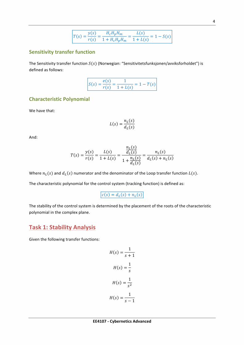
Characteristic Polynomial

We have that:

𝐿 𝑠 =𝑛!(𝑠)𝑑!(𝑠)

And:

𝑇 𝑠 =𝑦(𝑠)𝑟(𝑠)

=𝐿(𝑠)

1 + 𝐿(𝑠)=

𝑛!(𝑠)𝑑!(𝑠)

1 + 𝑛!(𝑠)𝑑!(𝑠)

=𝑛!(𝑠)

𝑑! 𝑠 + 𝑛! 𝑠

Where 𝑛!(𝑠) and 𝑑! 𝑠 numerator and the denominator of the Loop transfer function 𝐿(𝑠).

The characteristic polynomial for the control system (tracking function) is defined as:

𝑐 𝑠 = 𝑑! 𝑠 + 𝑛! 𝑠

The stability of the control system is determined by the placement of the roots of the characteristic polynomial in the complex plane.

Task 1: Stability Analysis

Given the following transfer functions:

𝐻 𝑠 =1

𝑠 + 1

𝐻 𝑠 =1𝑠

𝐻 𝑠 =1𝑠!

𝐻 𝑠 =1

𝑠 − 1

5


Task 1.1

Pen and paper: What are the poles for the different transfer functions above? Plot the poles in the imaginary plane. What are the stability properties of these systems (“asymptotically stable system”, “marginally stable system” or “unstable system”)?

Discuss the results.

Task 1.2

Do the same using MathScript.


Tip! Use the built-‐in functions poles and pzgraph.

Task 1.3

Plot the impulse responses of these systems using MathScript. Are they as expected?.

Tip! Use the built-‐in function impulse, which is similar to the step function we have used before.

Task 2: Stability Analysis of Feedback systems

Given the following feedback system:

The transfer function for the process is:

𝐻!(𝑠) =1

𝑠 + 1 !𝑠

The transfer function for the measurement/sensor is:

𝐻! 𝑠 = 𝐾! = 1

The transfer function for the controller is:

6


𝐻!(𝑠) = 𝐾!

We shall use 3 different values for 𝐾!:

𝐾! = 1

𝐾! = 2

𝐾! = 4

Task 2.1

Find 𝐿(𝑠), 𝑇(𝑠) and 𝑆(𝑠) for the system (both “pen and paper” and in MathScript).

Tip! In MathScript we can use the series and feedback functions in order to find 𝐿(𝑠) and 𝑇(𝑠).

Task 2.2

Plot the step response for the feedback system (𝑇(𝑠)).

Task 2.3

Find the poles and plot the poles in the imaginary plane for the feedback system (𝑇(𝑠)).

Is the system asymptotically stable, marginally stable system or unstable (for the 3 different values of 𝐾!)?


Task 3: Control System

Given the following control system:

The transfer functions are as follows:

7


𝐻! 𝑠 =𝐾!

𝑇!𝑠 + 1𝑒!!"

𝐻! 𝑠 =𝐾!

𝑇!𝑠 + 1𝑒!!"

𝐻! 𝑠 = 𝐾!

𝐻! 𝑠 = 𝐾!𝑇!𝑠 + 1𝑇!𝑠

Task 3.1

Find the loop transfer function 𝐿(𝑠), the tracking transfer function 𝑇(𝑠) and the sensitivity transfer function 𝑆(𝑠) for the system.

Task 4: Stability of Feedback systems

Given the following control system:

The transfer function for the process (including measurement) is:

𝐻!" =2𝑠

Task 4.1

Define the stability properties of this process (is the process stable or not?).

Task 4.2

The transfer function for the controller is:

𝐻! = 𝐾!

1. What is the loop transfer function 𝐿(𝑠)? 2. What is the tracking transfer function 𝑇(𝑠)? 3. What is the characteristic polynomial? 4. What is the systems pole(s)?

Task 4.3

8


For which values of 𝐾! is the system

• Asymptotically Stable • Unstable • Marginally stable?

Task 4.4

Define the system in MathScript and find the step response for the system for different values of 𝐾!.

Additional Resources

• http://home.hit.no/~hansha/?lab=mathscript

Here you will find tutorials, additional exercises, etc.

exercise 4 - stability analysis - telemark university...

Documents