experiment 7 - university of rochester

TA or TI Signature ___________________________________ 1 of 19

EXPERIMENT 7 Absolute Volt & Electrostatic

Potential

0. Pre-Lab Homework [2 pts]

1. In the first part of this lab you will be using a mechanically-balanced, axially-symmetric,

cylindrical capacitor to measure an absolute voltage. Each time you take a measurement,

but before you read the microscope scale, you should perform a critical procedural

technique. What is it, why is it critical, and how many times should you perform it?

(1 pt)

2. How do you determine the electric field lines for the second part of the experiment?

Electric fields are vector quantities. How will you determine the direction that they

should point? (1 pt)

Name: ___________________________ _____Date: _______________ Course number: _________ MAKE SURE YOUR TA OR TI STAMPS EVERY PAGE BEFORE YOU START!

Lab section: _____________ Partner's name(s): _________________ Grade:____________

Name___________________________________ Date: ________________ Course number: _________________

MAKE SURE TA & TI STAMPS EVERY PAGE BEFORE YOU START



Potential

1. Purpose

The purpose is to calculate an absolute voltage measurement by mechanical means and illustrate

the concepts of the electric field by means of experimental demonstration.

2. Introduction

A force (given by Coulomb's Law) is exerted on a particular electric charge by every other

charge. The total electrical force acting on such a charge is the sum of all these forces. If a

small charge were introduced to "test" it, the force on this test charge would be found to vary as

it was moved around.

Considerations such as these give rise to the concept of a field. An electric field is the force

per unit charge at any position in space, that is independent of the test charge and is a

characteristic of the spatial distribution of charge in the region.. The electric field can be thought

of as the capacity for producing an electric force on a charge. Conceptually, the electric field is

well defined at any place even though there may not actually be any test charge there to

experience it.

If a test charge is moved around in an electric field, the electric force will do work on it. The

static electrical force of Coulomb's law is a conservative force. That is, the work done moving

between two points is independent of the path taken. This suggests another useful concept,

electric potential. The potential difference between two points is the work per unit charge that

would be done by the electric field in moving a test charge between them.

This laboratory experiment should help the student gain a concrete grasp of these abstract

concepts and facilitate understanding of capacitance and the connection between force, distance

and energy in the context of electrical phenomena.

In the first part of this experiment, you will relate an electrical potential to mechanical

quantities using an indirect method to make an absolute voltage measurement. This method,

through clever design, avoids the worst of the systematic errors from which a direct Coulomb's

Law experiment suffers and yields more precise results. In the second part, you will investigate

static electric fields and map out their equipotential surfaces.




3. Laboratory Work

3.1 Absolute Measurement of Voltage

Introduction

An absolute measurement of electrical potential difference by mechanical means is a

way to learn about electrical quantities and relate them to mechanical ones that are already

known.

The study of electricity and magnetism normally begins after a thorough introductory

study of mechanics. The first important electrical relationship encountered is Coulomb's

law, which says that the force acting between two point charges is proportional to their

magnitudes and inversely proportional to the square of the distance between them. Once the

constant of proportionality has been chosen the unit of charge has in principle been defined

for that system of units (i.e. mks). Then, in order to measure charge one would simply set

up two identical point charges a known distance apart, measure the force between them and

then use Coulomb's law to get the magnitude of the charges.

But making a direct and accurate measurement of Coulomb's law is not readily feasible.

The required point charges are not available, and the distribution of charges on conducting

spheres (such as one might try to use in practice) is not uniform. The distribution of charge

depends in a complicated way on the position of all local objects, conducting or non-

conducting, charged or not charged.

Fortunately, a practical way exists to determine an electrical quantity in terms of force,

by making an "absolute" measurement, using a method based upon capacitance.

The Concept of Capacitance

Since the charge on an electrical conductor distributes itself so as to form an equipotential,

there is a certain value of electrical potential associated with each conductor. And, because

electrostatic fields superimpose, these potentials will be linearly related to the charges on the

conductors. The concept of capacitance describes the coefficients of these relationships,

which are determined only by system geometry.

In a system of two conductors carrying opposite charges of magnitude Q, this relationship

is simply,

C = Q/ V Equation 7.1

where V is the voltage (potential difference) between them, and the coefficient C is their

mutual capacitance. A simple example is the parallel plate capacitor, which has a

capacitance in air (neglecting edge effects) of,

Equation 7.2

0 (= 8.854 10-12 C2//N-m2) is the dielectric constant of free space.

C oA

d(m.k.s.units)




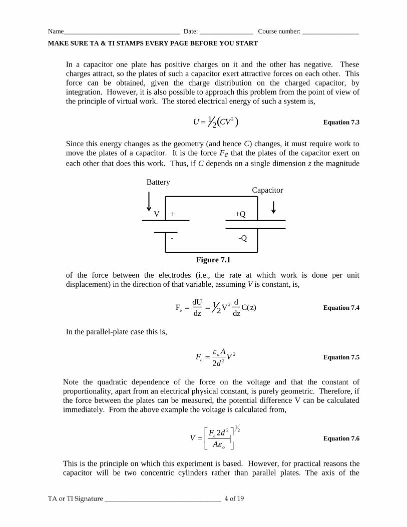
In a capacitor one plate has positive charges on it and the other has negative. These

charges attract, so the plates of such a capacitor exert attractive forces on each other. This

force can be obtained, given the charge distribution on the charged capacitor, by

integration. However, it is also possible to approach this problem from the point of view of

the principle of virtual work. The stored electrical energy of such a system is,

Equation 7.3

Since this energy changes as the geometry (and hence C) changes, it must require work to

move the plates of a capacitor. It is the force Fe that the plates of the capacitor exert on

each other that does this work. Thus, if C depends on a single dimension z the magnitude

of the force between the electrodes (i.e., the rate at which work is done per unit

displacement) in the direction of that variable, assuming V is constant, is,

Equation 7.4

In the parallel-plate case this is,

2

22V

d

AF o

e

Equation 7.5

Note the quadratic dependence of the force on the voltage and that the constant of

proportionality, apart from an electrical physical constant, is purely geometric. Therefore, if

the force between the plates can be measured, the potential difference V can be calculated

immediately. From the above example the voltage is calculated from,

2

122

o

e

A

dFV

Equation 7.6

This is the principle on which this experiment is based. However, for practical reasons the

capacitor will be two concentric cylinders rather than parallel plates. The axis of the

U 12 CV

2

Fe dU

dz 1

2V2 d

dzC(z)

Figure 7.1

Capacitor

+Q

-Q

V +

-

Battery




cylinders will be in the same direction as the force (+z). Of course, the capacitance between

the two cylinders will be different from the capacitance of the parallel plate, the example

shown above, but capacitance depends only on system geometry. This is discussed below.

The Experimental Apparatus

The apparatus shown in Figure 7.2 is designed for measuring the axial force in the vertical

direction between two concentric aluminum circular cylinders. The potential difference is

determined across these two cylinders where up to 3,000 V is applied. The outer cylinder of

the capacitor is fixed in the semicircular ends of two Lucite plates. The inner cylinder,

which must be quite uniform and light in weight, is made from a cleaned beverage can.

This inner cylinder moves vertically, supported by a thin shaft constrained by two bearings.

These bearings must run freely; so they must be kept clean. If a bearing begins to rub or

grab it can be washed out with alcohol and then lubricated with a small single drop of

spindle oil. The lower end of the shaft is supported by a hollow float partially submerged in

water. Distilled water with a few drops of Eastman Kodak Photo-Flo 200 wetting agent will

reduce surface tension. The fully submerged main body of the float, a ping-pong ball (of

unknown compressibility) provides most of the buoyancy required to support the shaft and

its load. The submerged portion of the glass tube connecting the ball to the shaft supplies the

rest.

The net vertical force on the movable part of the experiment is,

Equation 7.7

is the electrical force between the cylindrical capacitors, non-zero when a potential is

applied; is the upward buoyancy force of the ping-pong ball, and is the downward

force of gravity. The idea is for and to almost cancel each other so that dominates.

When a potential is applied, the electrical force will be balanced by any change in the

buoyant force, Fb.

The (vertical) equilibrium position is set by the water level in the beaker and the small

weights (brass or steel nuts) in the weight pan. The weights should be used to adjust the

immersion of the float so that the surface of the water is level with the center of the rod. The

water level should be adjusted so that the can clears the top bearing by about a centimeter.

The system will be displaced from equilibrium by any force between the cylinders. The

position of the system is observed through a low-power microscope directed at an optical

target on the shaft.

The can is connected to ground via the bearings; the outer cylinder is connected to the

potential source through a protective (high voltage) resistance of several tens of mega-ohms.

Although this high voltage is exposed, the resistor prevents any significant current from

F Fe Fb Fg

Fe

Fb Fg

Fb Fg Fe




flowing; it is not dangerous, although it may be uncomfortable if touched. Therefore, do

not touch the can, which could be at 3000 Volts.

The can and cylinder overlap for a length much greater than the radial spacing between

them, and the cylinder extends well beyond the upper end of the can. Under these

conditions the change in capacitance produced by a small axial position shift s will, to a

very good approximation, be given simply by,

Equation 7.8

where is the capacitance per unit length of a long cylindrical capacitor and given by,

1

2ln

2

rr

o Equation 7.9

where r1 is the radius of the beverage can, and r2 is the radius of the cylinder. These

equations are valid because the electrical field distribution in most of the overlap region is

essentially invariant axially; and also the end effects will be quite small due to the favorable

geometry (the cylinder extends well beyond the can above and the can extends well beyond

the cylinder below).

Accordingly, for a potential difference V between the electrodes, the change in energy

storage with displacement may be written,

C s

These are typical dimensions

for the apparatus. The dimensions

of your apparatus may be slightly

different.

Radius of beverage can

r1 = 2.647cm

Radius of cylinder

r2 = 2.907cm

Diameter of the float stem

d = 0.7cm

Diameter of water vessel

D = 8.57cm

Figure 7.2

weight pan

microscope

floatleveling

screw

optical target

spring clip

level

target stop




sV

rr

VsCVU o 2

1

2

22

ln2

1

2

1

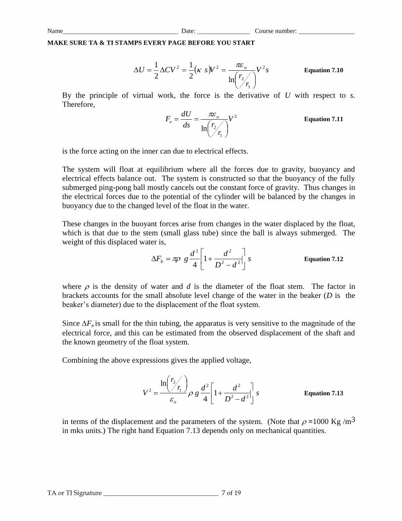
Equation 7.10

By the principle of virtual work, the force is the derivative of U with respect to s.

Therefore,

2

1

2ln

V

rrds

dUF o

e

Equation 7.11

is the force acting on the inner can due to electrical effects.

The system will float at equilibrium where all the forces due to gravity, buoyancy and

electrical effects balance out. The system is constructed so that the buoyancy of the fully

submerged ping-pong ball mostly cancels out the constant force of gravity. Thus changes in

the electrical forces due to the potential of the cylinder will be balanced by the changes in

buoyancy due to the changed level of the float in the water.

These changes in the buoyant forces arise from changes in the water displaced by the float,

which is that due to the stem (small glass tube) since the ball is always submerged. The

weight of this displaced water is,

sdD

ddgFb

22

22

14

Equation 7.12

where is the density of water and d is the diameter of the float stem. The factor in

brackets accounts for the small absolute level change of the water in the beaker (D is the

beaker’s diameter) due to the displacement of the float system.

Since Fb is small for the thin tubing, the apparatus is very sensitive to the magnitude of the

electrical force, and this can be estimated from the observed displacement of the shaft and

the known geometry of the float system.

Combining the above expressions gives the applied voltage,

sdD

ddg

rr

Vo

22

221

2

2 14

ln

Equation 7.13

in terms of the displacement and the parameters of the system. (Note that =1000 Kg /m3

in mks units.) The right hand Equation 7.13 depends only on mechanical quantities.




Procedure

CAUTION: Do NOT touch the can. Although the available power is too small to be

dangerous, potentials of several thousand volts are involved here so touching the cylinder

may be uncomfortable. Also, if it gets dirty the experiment may fail.

1. Check to see if the water level is about halfway up the glass stem of the float; if not, add

or remove weights to make it so. Check to see that the can clears the upper bearing

properly (about 1 cm). If it is necessary, add or remove water.

For accurate and reproducible measurements the shaft must be able to freely assume its

proper position. Even when the bearings are well aligned and the shaft is essentially

vertical, bearing friction will interfere with the necessary free movement. This can be

overcome by setting the system spinning by gentle use of thumb and forefinger on the

shaft. Steady your hand by resting it lightly on the bearing support while doing this.

Make sure your hands are clean when spinning the shaft, wash them if necessary.

2. Fiddle with the apparatus to become familiar with it. Try spinning the shaft gently

using (clean and dry) thumb and forefinger. Once started, spinning should persist for five

or ten seconds and should gradually die out rather than come to a sudden stop. Check to

see if your apparatus behaves this way; if not the bearings need to be cleaned and you

should get your TA to help.

Important: Every time you make a change you must spin the shaft to overcome the

friction. Do this at least –twice- to confirm that you are obtaining an accurate reading.

3. Remove the microscope from the apparatus and hold it up to the light. Observe the

scale on the lens of the microscope. The scale is 6mm long with large divisions of 1mm

and small divisions of .1mm. It may be helpful to hold the microscope a few inches away

from your eye. Replace the microscope into the apparatus.

3.1 Focus the microscope so that the target and scale can both be seen clearly while

looking through the microscope. Focusing is achieved by moving the microscope in or

out. If necessary, reset the optical target by loosening the small screw on the target stop,

centering the target on the scale, then retightening the small screw. Spin the shaft and

observe how the target settles into position. Repeat, checking for consistency.

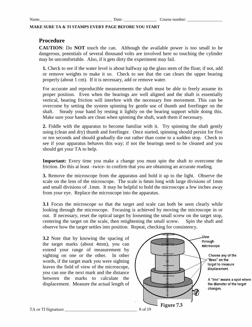
3.2 Note that by knowing the spacing of

the target marks (about 4mm), you can

extend your range of measurement by

sighting on one or the other. In other

words, if the target mark you were sighting

leaves the field of view of the microscope,

you can use the next mark and the distance

between the marks to calculate the

displacement. Measure the actual length of

Figure 7.3




your target so you can do this (see Figure 7.3).

Calibrate Displacement vs. Voltage

4. Apply five different voltages as indicated by the power supply meter to the apparatus,

ranging up to near 3000V. Suggested voltages are: 0, 1000, 2000, 2500, 3000 Volts.

Again spin the shaft at least twice after changing the voltage to make sure you are getting

the consistent measurements. Measure the displacement of the optical target mark from

one voltage to the next. Record your displacement readings for each voltage change in

Table 7.1 located in Section 4.1.

Measure a Voltage Using the Theoretical Sensitivity

5. Set your power supply to some intermediate voltage (i.e. 2200 Volts). Record this

value in Section 4.1. We will treat this measurement as the “unknown” voltage, and try to

determine it in two different ways: first from the method in Step 4 and second (the ‘null’

method) from Steps 9 – 11.

6. Switch the power supply off (to ground) and note the microscope scale reading.

7. Then switch back on the power supply and record the microscope scale reading.

Subtract to get the displacement, s. Record the displacement data in Table 7.2.

8. Repeat this measurement several times, recording your measurements in Table 7.2.

Then average the measured values to determine savg

Measure a Voltage Using the “Null Method“

9. Without changing the power supply voltage (i.e. use the same “unknown voltage”), find

another value for the applied voltage by use of a “null method”. With the power supply

off or disconnected, note a "zero" point on the microscope scale.

10. Then apply the voltage from the power supply (i.e. 2200 Volts).

11. Keeping careful track, add masses until the zero point has been passed, then

interpolate to find the mass corresponding to scale zero. Calculate the force Fnull due to

this mass and record this force in the space provided in Section 4.1.

--------Switch off all POWER when you are done.--------

3.2 Electric Field Mapping

Introduction




In this experiment you will investigate the electric potentials set up by electrodes that cause

currents to flow in conductive sheets. You will be able to map out the equipotential

contours and find the electric field lines for several configurations of electrodes.

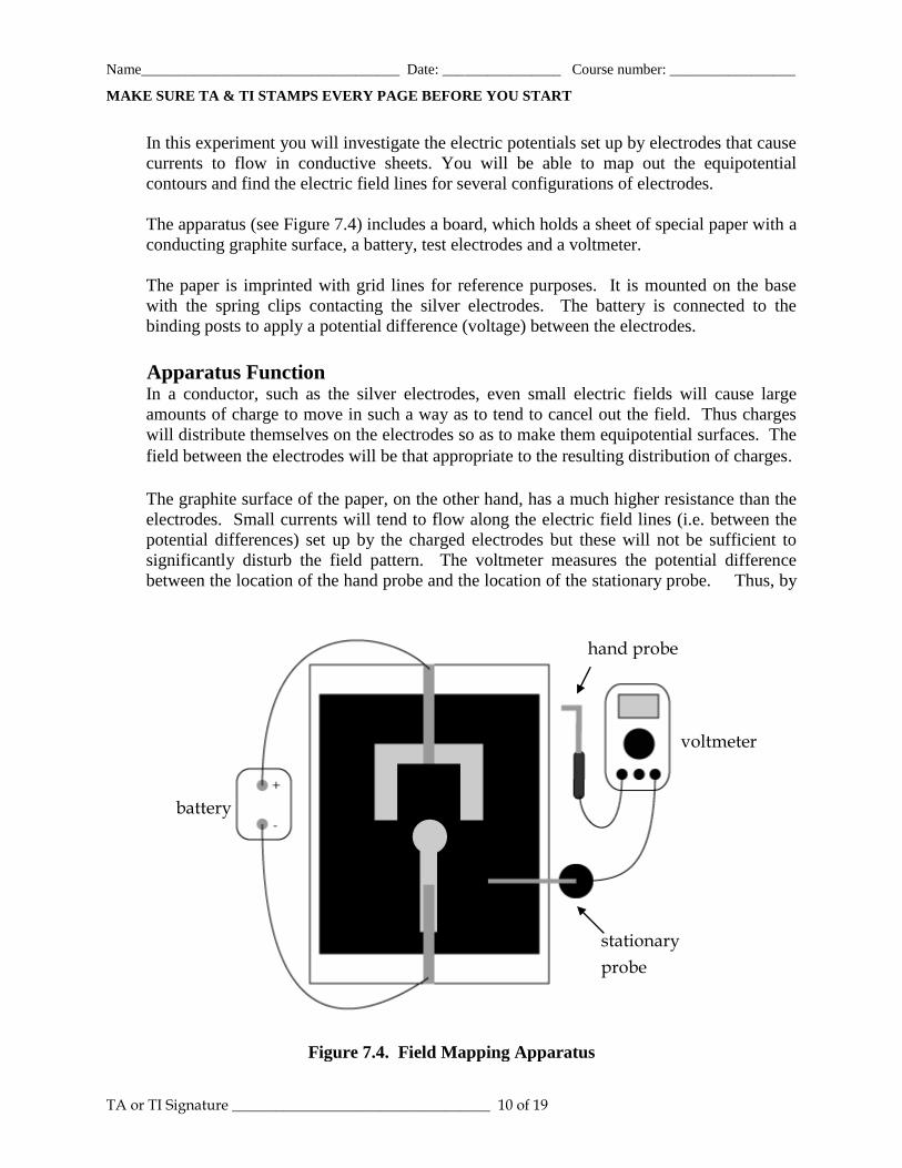
The apparatus (see Figure 7.4) includes a board, which holds a sheet of special paper with a

conducting graphite surface, a battery, test electrodes and a voltmeter.

The paper is imprinted with grid lines for reference purposes. It is mounted on the base

with the spring clips contacting the silver electrodes. The battery is connected to the

binding posts to apply a potential difference (voltage) between the electrodes.

Apparatus Function In a conductor, such as the silver electrodes, even small electric fields will cause large

amounts of charge to move in such a way as to tend to cancel out the field. Thus charges

will distribute themselves on the electrodes so as to make them equipotential surfaces. The

field between the electrodes will be that appropriate to the resulting distribution of charges.

The graphite surface of the paper, on the other hand, has a much higher resistance than the

electrodes. Small currents will tend to flow along the electric field lines (i.e. between the

potential differences) set up by the charged electrodes but these will not be sufficient to

significantly disturb the field pattern. The voltmeter measures the potential difference

between the location of the hand probe and the location of the stationary probe. Thus, by

Figure 7.4. Field Mapping Apparatus

voltmeter

hand probe

battery

stationary

probe




finding points between which the voltmeter measures zero, you can map out contours with

the same potential.

Procedure

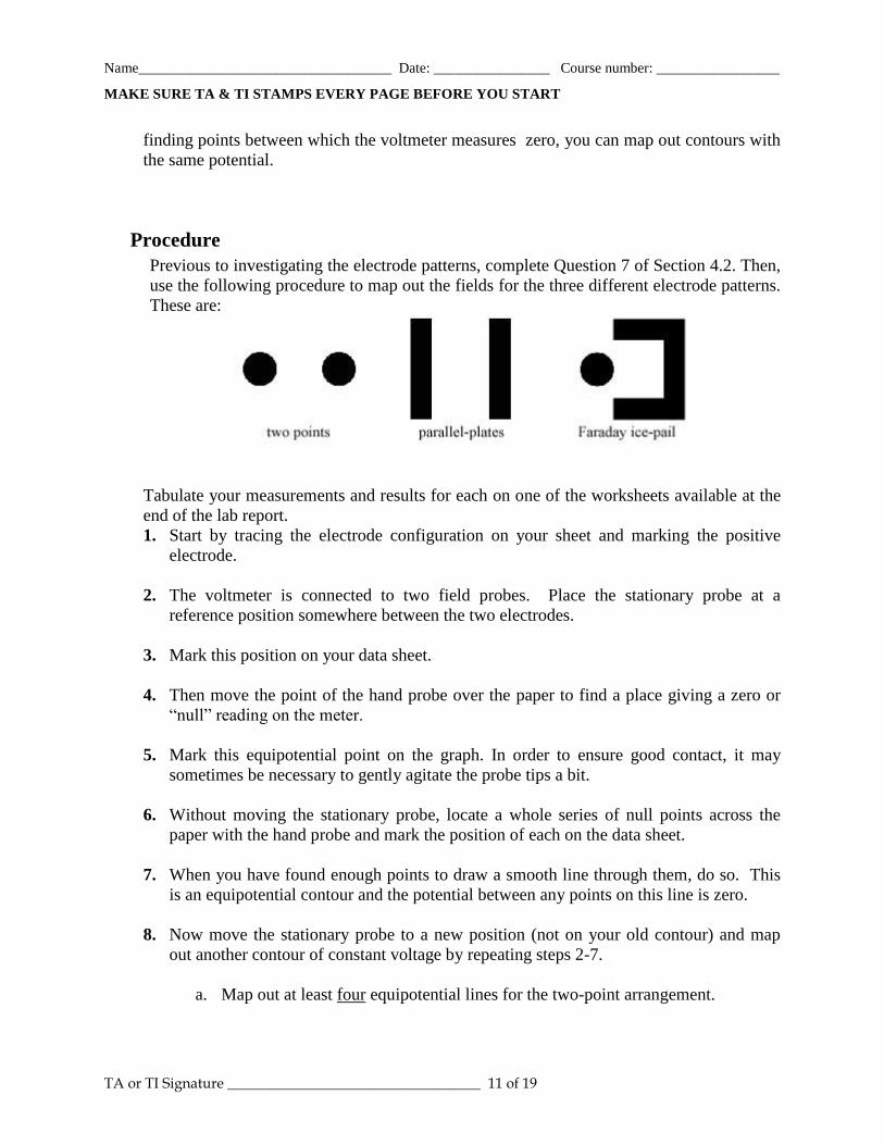
Previous to investigating the electrode patterns, complete Question 7 of Section 4.2. Then,

use the following procedure to map out the fields for the three different electrode patterns.

These are:

Tabulate your measurements and results for each on one of the worksheets available at the

end of the lab report.

1. Start by tracing the electrode configuration on your sheet and marking the positive

electrode.

2. The voltmeter is connected to two field probes. Place the stationary probe at a

reference position somewhere between the two electrodes.

3. Mark this position on your data sheet.

4. Then move the point of the hand probe over the paper to find a place giving a zero or

“null” reading on the meter.

5. Mark this equipotential point on the graph. In order to ensure good contact, it may

sometimes be necessary to gently agitate the probe tips a bit.

6. Without moving the stationary probe, locate a whole series of null points across the

paper with the hand probe and mark the position of each on the data sheet.

7. When you have found enough points to draw a smooth line through them, do so. This

is an equipotential contour and the potential between any points on this line is zero.

8. Now move the stationary probe to a new position (not on your old contour) and map

out another contour of constant voltage by repeating steps 2-7.

a. Map out at least four equipotential lines for the two-point arrangement.




b. Map out at least four equipotential lines for the parallel plates arrangement. Be

sure you probe beyond the edges of the plates to notice interesting patterns

there.

c. Map out at least four equipotential lines for the Faraday Ice-pail pattern. Two

of these lines should examine the inside of the “pail.” Sketch as many

equipotentials as is necessary to show its interesting structure. In the Faraday’s

ice-pail pattern, start your examination by putting the stationary probe near the

bottom of the "pail."

9. The electric field is everywhere perpendicular to the equipotentials. Sketch in with

dashed lines on your data sheets examples of how the electric field lines (lines of force)

must run. Be sure to do this in the interesting parts of the pattern. Remembering that

the electric field is a vector, indicate with arrows the direction associated with the

electric field lines.

10. BE SURE TO DISCONNECT THE BATTERY AND TURN OFF THE

VOLTMETER WHEN YOU ARE DONE!

REFERENCE:

H.W. Fullbright, “A Simple and Inexpensive Teaching Apparatus For Absolute

Measurement of Voltage”, American Journal Physics, v.61, pp. 896-900, Oct. 1993.


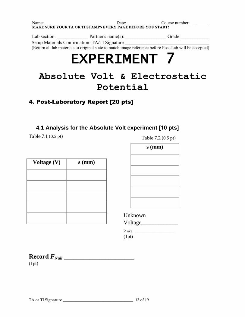
Table 7.2 (0.5 pt)


Potential

4. Post-Laboratory Report [20 pts]

4.1 Analysis for the Absolute Volt experiment [10 pts]

Table 7.1 (0.5 pt)

Record FNull ______________________(1pt)

Voltage (V) s (mm)

s (mm)

Unknown

Voltage_____________

s avg ______________

(1pt)

Name: ___________________________ _____Date: _______________ Course number: _________ MAKE SURE YOUR TA OR TI STAMPS EVERY PAGE BEFORE YOU START!

Lab section: _____________ Partner's name(s): _________________ Grade:____________Setup Materials Confirmation: TA/TI Signature ___________________________________ (Return all lab materials to original state to match image reference before Post-Lab will be accepted)




1. Make a plot of the data from Table 7.1 of Displacement vs. Volts2 (note the squared Voltage!) Draw a best-fit straight line and measure its slope. Show your calculation and include units. Include a label with units identified for each axes. (2 pts)




2. Using the slope found in the graph above (in mm/V2) and the average value of

displacement from Table 7.2, calculate the “unknown” voltage. Compute the percent

error using this value and the known value. (1 pt)

3. Using Equation 7.11 and the balancing force, FNull, calculate the “unknown” voltage

again. Here only stability of the zero point is required; the buoyant force does not appear

in the calculation. (1 pt)




4. What is the limiting experimental parameter for measuring an unknown voltage in each

measurement? (In other words, what variable in Eq.7.13 has the greatest uncertainty?)

(2pts)

displacement measurement?

null method measurement?

5. Finally, which method of measurement is more reliable? Why? Be specific. (1 pt)

4.2 Analysis for the Electric Field Mapping Experiment [10 pts]

6. Draw the electric field lines you would expect for the point charge below. Identify two

arbitrary regions of the electric field and label which one is stronger. State how can you

determine this from the field lines (1pt)

+q




4.2.1 Two-Point Pattern Data Sheet

7. Sketch in the electric field lines according to your measured mapping of equipotential surfaces. Be sure to include arrows to show the direction of your field lines. (2 pts)

8. In which region(s) would the electric force on a test charge be the largest? Why? (1pt)




4.2.2 Parallel Plate Pattern Data Sheet

9. Sketch in the electric field lines according to your measured mapping of equipotential

surfaces. Be sure to include arrows to show the direction of your field lines. (2 pts)

10. Describe the trajectory of a positive unit charge if it were introduced midway between the

plates with a velocity directed parallel to the plates. Draw a figure if you desire. (1 pt)




4.2.3 Faraday’s Ice-Pail Pattern Data Sheet

11. Sketch in the electric field lines according to your measured mapping of equipotential

surfaces. Be sure to include arrows to show the direction of your field lines. (2 pts)

12. Is the electric field inside the pail larger or smaller than outside? Why? (1pt)

(Hint : where does the potential change the fastest? 𝐸 = −∇∅ )

experiment 7 - university of rochester

Documents