experimental evidence on the effects of home computers on

211

American Economic Journal: Applied Economics 2013, 5(3): 211–240 http://dx.doi.org/10.1257/app.5.3.211

Experimental Evidence on the Effects of Home Computers on Academic

Achievement among Schoolchildren†

By Robert W. Fairlie and Jonathan Robinson*

Computers are an important part of modern education, yet many schoolchildren lack access to a computer at home. We test whether this impedes educational achievement by conducting the largest-ever field experiment that randomly provides free home computers to students. Although computer ownership and use increased substantially, we find no effects on any educational outcomes, including grades, test scores, credits earned, attendance, and disciplinary actions. Our estimates are precise enough to rule out even modestly-sized positive or negative impacts. The estimated null effect is consistent with survey evidence showing no change in homework time or other “intermediate” inputs in education. (JEL I21, I24, J13)

Computers are an important part of modern education. In the United States, schools spend more than $5 billion per year on computers and information technology

(Market Data Retrieval (MDR) 2004), while the federal government spends another $2 billion per year on the E-rate program, which provides discounts to low-income schools and libraries (Universal Service Administration Company 2010). A large share of these expenditures goes toward in-school computing, and, consequently, access to computers in school is ubiquitous.1 In contrast, many children do not have access to a computer at home. Nearly 9 million children ages 10–17 in the United States (27 percent) do not have computers with Internet connections at home (National Telecommunications and Information Administration (NTIA) 2011). Partly to address these disparities, and to further reduce computer-to-student ratios in the classroom,

1 There are an estimated 15.5 million instructional computers in US public schools, representing one instruc-tional computer for every three schoolchildren. Nearly every instructional classroom in these schools has a com-puter, averaging 189 computers per school (US Department of Education 2011a).

* Fairlie: Department of Economics, University of California, Santa Cruz, CA 95064 (e-mail: [email protected]); Robinson: Department of Economics, University of California, Santa Cruz, CA 95064 (e-mail: [email protected]). We thank Computers for Classrooms, Inc., the ZeroDivide Foundation, and the NET Institute (www.NETinst.org) for generous funding for the project. We thank David Card, Tarjei Havnes, Oded Gurantz, and participants at seminars and workshops at UC Berkeley, SOLE, the MacArthur Foundation and the CESifo ICT Conference for comments and suggestions. We also thank Jennifer Bevers, Bruce Besnard, John Bohannon, Linda Coleman, Reg Govan, Rebecka Hagerty, Kathleen Hannah-Chambas, Brian Gault, David Jansen, Cynthia Kampf, Gina Lanphier, Linda Leonard, Kurt Madden, Lee McPeak, Stephen Morris, Joanne Parsley, Richard Pascual, Jeanette Sanchez, Zenae Scott, Tom Sharp, and many others for administering the program in schools. We thank Shilpa Aggarwal, Julian Caballero, David Castaneda, James Chiu, Samantha Grunberg, Keith Henwood, Cody Kennedy, Nicole Mendoza, Nick Parker, Miranda Schirmer, Glen Wolf and Heidi Wu for research assistance. Finally, special thanks go to Pat Furr for donating many computers for the study and distributing computers to schools.

† Go to http://dx.doi.org/10.1257/app.5.3.211 to visit the article page for additional materials and author disclosure statement(s) or to comment in the online discussion forum.

http://dx.doi.org/10.1257/app.5.3.211

mailto:[email protected]




www.NETinst.org

www.NETinst.org


212 AmEriCAn ECOnOmiC JOurnAL: AppLiEd ECOnOmiCs JuLy 2013

a growing number of schools are implementing costly one-to-one laptop programs (Silvernail et al. 2011; Texas Center for Educational Research 2009; Lowther 2007).2 These programs are extremely expensive. For example, equipping each of the 55.5 million public school students in the United States with a laptop would cost tens of billions of dollars even if these laptops were replaced only every 3 years.

How important is this disparity in access to home computing to the educational achievement of schoolchildren, especially given the pervasiveness of computers in the US classroom? The potential impact depends on why households do not have computers in the first place. If households are rational and face no other frictions, those households without computers have decided not to buy a computer because the returns are relatively low. Although home computers are useful for completing school assignments through word processing, research, spreadsheets, and other edu-cational uses, they also provide a distraction caused by game, social networking, and other entertainment use.3 However, it is also possible that various constraints prevent households from investing in home computers, even if the returns are high. For exam-ple, parents may simply be unaware of the returns to computer use, or they may face credit constraints. There is reason to suspect that these constraints might be impor-tant, given that households without computers tend to be substantially poorer and less educated than other households (National Telecommunication and Information Administration 2011). Thus, the effect of computers for such families is an open and important question.

Only a few studies have examined this question, and there is no consensus in this literature on whether the effects of home computers are positive or negative. A few studies find large positive effects of home computers on various educational outcomes, such as grades, test scores and cognitive skills (Attewell and Battle 1999; Fiorini 2010; Schmitt and Wadsworth 2006; Fairlie 2005; Fairlie, Beltran, and Das and 2010; Malamud and Pop-Eleches 2011), and an almost equal number of studies find evidence of modestly-sized to large negative effects of home computers on edu-cational outcomes (Fuchs and Woessmann 2004; Vigdor and Ladd 2010; Malamud and Pop-Eleches 2011). Thus, it remains an open question as to whether home com-puters are academically beneficial or harmful to schoolchildren.4

2 Extensive efforts to provide laptops to schoolchildren also exist in many developing countries. For example, the One Laptop per Child program has provided more than 2 million computers to schools in Uruguay, Peru, Argentina, Mexico, and Rwanda, and new projects in Gaza, Afghanistan, Haiti, Ethiopia, and Mongolia. See http://one.laptop.org/about/countries.

3 Surveys of home computer use among schoolchildren indicate high levels of use for both schoolwork and enter-tainment (see, for example, Lenhart et al. 2008; Lenhart 2009; Pew Internet Project 2008a, b; US Department of Education 2011a; Kaiser Family Foundation 2010). Theoretically, there is also no clear prediction of whether the net effects are positive or negative (see Fairlie, Beltran, and Das 2010, for example).

4 A larger and more established literature examines the impacts of computers and computer-assisted software in schools (where use is regulated by teachers) and finds somewhat mixed results ranging from null to large posi-tive impacts. See Kirkpatrick and Cuban (1998) and Noll et al. (2000) for earlier reviews of the literature, and see Barrera-Osorio and Linden (2009) and Cristia et al. (2012) for more recent evidence on computer impacts in schools. See Goolsbee and Guryan (2006) and Machin, McNally and Silva (2007) for evidence on the effects of ICT expenditures and subsidies to schools, and Angrist and Lavy (2002); Banerjee et al. (2007); Barrow, Markman and Rouse (2009); and Carrillo, Onofa and Ponce (2010) for evidence on computer-assisted software in schools. These results contrast with stronger evidence of positive effects for other school inputs, such as teacher quality (e.g., Rivkin, Hanushek, and Kain 2005).

http://one.laptop.org/about/countries

http://one.laptop.org/about/countries

VOL. 5 nO. 3 213Fairlie and robinson: Computers and aCademiC aChievement

Empirically, the key challenge in the literature is isolating the causal effect of home computers from other unobserved differences across students and their families. Previous studies address concerns about possible omitted variable bias (mainly due to selection) by controlling for detailed student and family background characteris-tics, instrumenting for computer ownership, performing falsification tests, and/or esti-mating fixed effect models (for example, see Attewell and Battle 1999; Fiorini 2010; Schmitt and Wadsworth 2006; Fuchs and Woessmann 2004; Fairlie 2005; Vigdor and Ladd 2010; Fairlie, Beltran, and Das 2010). More recently, to address selection bias, Malamud and Pop-Eleches (2011) estimate a regression discontinuity design using a computer voucher program for low-income families in Romania. Their estimates indi-cate negative effects of having a home computer on grades, but positive effects on cognitive and computer skills. The only randomized experiment examining the impacts of home computers of which we are aware was conducted by one of the authors with a sample of 286 low-income community college students (Fairlie and London 2012).5 That study found evidence of small positive effects on educational outcomes for college students, but did not estimate impacts on schoolchildren, which may differ greatly.6

We provide evidence on the educational impacts of home computers by conduct-ing a randomized control experiment with 1,123 students in grades 6–10 attending 15 schools across California. It represents the first field experiment involving the provision of free computers to schoolchildren for home use ever conducted, and the largest experiment involving the provision of free home computers to students at any level. All of the students participating in the study did not have computers at base-line. Half were randomly selected to receive free computers, while the other half served as the control group. Since the goal of the study was to evaluate the effects of home computers alone, instead of a broader technology policy intervention, no training or other assistance was provided. At the end of the school year, we obtained administrative data from schools to test the effects of the computers on numerous educational outcomes. The reliance on school-provided administrative data avail-able for almost all students for the main education outcomes essentially eliminates concerns over attrition bias and measurement error. We supplement this information with a detailed follow-up survey, which includes information on computer use and homework effort, in addition to other outcomes.

5 A few randomized control experiments have recently been conducted to examine the effectiveness of com-puter-assisted instruction in schools (e.g., Barrow, Markman and Rouse 2009; Mathematica 2009; Banerjee et al. 2007; Barrera-Osorio and Linden 2009) and laptop use in schools (Cristia et al. 2012). Although the One Laptop per Child program in Peru (Cristia et al. 2012) and the Texas laptop program (evaluated with a quasi-experiment in Texas Center for Educational Research 2009) were initially intended to allow students to take computers home when needed in addition to using them in school, this did not happen in most cases. In Peru, some principals, and even parents, did not allow the computers to come home because of concerns that the laptops would not be replaced through the program if they were damaged or stolen. The result is that only 40 percent of students took the laptops home, and home use was substantially lower than in-school use. In Texas, there were similar concerns resulting in many schools not allowing computers to be taken home or restricting their home use. The main effect from these laptop programs is therefore to provide one computer for every student in the classroom, rather than to increase home access.

6 From an analysis of matched CPS data, the study finds estimates of impacts of home computers on community college students that are nearly an order of magnitude larger than the experimental estimates raising concerns about potential biases in non-experimental estimates (Fairlie and London 2012).


We find that even though the experiment had a large effect on computer ownership and total hours of computer use, there is no evidence of an effect on a host of edu-cational outcomes, including grades, standardized test scores, credits earned, atten-dance, and disciplinary actions. We do not find effects at the mean, important cutoffs in the distribution (e.g., passing and proficiency), or quantiles in the distribution. Our estimates are precise enough to rule out even moderately-sized positive or nega-tive effects. Evidence from our detailed follow-up survey supports these findings. We find no evidence that treatment students spent more or less time on homework, and we find that the computers had no effect on turning homework in on time, soft-ware use, computer knowledge, and other intermediate inputs in education. The pat-tern of time usage is also consistent with a negligible effect of the computers—while treatment students did report spending more time on computers for schoolwork, they also spent more time on games, social networking, and other entertainment. Children also report relatively few hours spent doing homework overall, which may have limited the potential for the computers to increase the productivity of their homework even if effective. Finally, we find no evidence of heterogeneous treatment effects by pretreatment academic achievement, parental supervision, propensity for nongame use, or major demographic characteristics. Overall, these results suggest that increasing access to home computers among students who do not already have access is unlikely to greatly improve educational outcomes, but is also unlikely to negatively affect outcomes.7

The remainder of the paper is organized as follows. In Section I, we describe the computer experiment in detail and present a check of baseline balance between the treatment and control groups. Section II presents our main experimental results. Section III presents results for heterogeneous treatment effects. Section IV concludes.

I. Experimental Design

A. sample

The sample for this study includes students enrolled in grades 6–10 in 15 differ-ent middle and high schools in 5 school districts in California. Middle school stu-dents comprise the vast majority of the sample.8 We focus on this age group because younger students (i.e., elementary school students) would likely have less of a need to use computers for schoolwork and because middle school captures a critical time in the educational process for schoolchildren prior to, but influencing later, deci-sions about taking college prep courses and dropping out of school. The project took place over 2 years: 2 schools participated in 2008–2009, 12 schools participated in 2009–2010, and 1 school participated in both years. The 15 schools in the study span the Central Valley of California geographically. Overall, these schools are similar in

7 The negative effects of home computers have gained a fair amount of attention recently in the press. See, for example, “Computers at Home: Educational Hope versus Teenage Reality,” new york Times, July 10, 2010 and “Wasting Time Is New Divide in Digital Era,” new york Times, May 29, 2012.

8 The distribution of grade levels is as follows: 9.5 percent grade 6, 47.8 percent grade 7, 39.9 percent grade 8, and 2.8 percent grades 9 and 10.


size (749 students compared to 781 students), student to teacher ratio (20.4 to 22.6), and female to male student ratio (1.02 to 1.05) as California schools as a whole (US Department of Education 2011b). Our schools, however, are poorer (81 percent free or reduced price lunch compared with 57 percent) and have a higher percentage of minority students (82 percent to 73 percent) than the California average. They also have lower average test scores than the California average (3.2 compared with 3.6 in English-language arts and 3.1 compared with 3.3 in math), but the differences are not large (California Department of Education 2010). Although these differences may impact our ability to generalize the results, low-income, ethnically diverse schools such as these are the ones most likely to enroll schoolchildren without home computers and be targeted by policies to address inequalities in access to technology (e.g., E-rate program and IDAs).

To identify children who did not have home computers, we conducted an in-class survey at the beginning of the school year with all of the students in the 15 participating schools. The survey, which took only a few minutes to complete, asked basic questions about home computer ownership and usage. To encourage honest responses, it was not announced to students that the survey would be used to determine eligibility for a free home computer (even most teachers did not know the purpose of the survey). Responses to the in-class survey are tabulated in Appendix Table A1. In total, 7,337 students completed in-class surveys, with 24 percent reporting not having a computer at home. This rate of home computer ownership is roughly comparable to the national average. Estimates from the 2010 CPS indicate that 27 percent of children aged 10–17 do not have a computer with Internet access at home (US Department of Education 2011a).

Any student who reported not having a home computer was eligible for the study.9 In discussing the logistics of the study with school officials, school princi-pals expressed concern about the fairness of giving computers to a subset of eligible children. For this reason, we decided to give out computers to all eligible students. Treatment students received computers immediately, while control students had to wait until the end of the school year. Our main outcomes are all measured at the end of the school year, before the control students received their computers.

All eligible students were given an informational packet, baseline survey, and consent form to complete at home. To participate, children had to have their par-ents sign the consent form (which, in addition to participating in the study, released future grade, test score, and administrative data) and return the completed survey to the school. Of the 1,636 students eligible for the study, we received 1,123 responses with valid consent forms and completed questionnaires (68.6 percent).10

9 Because eligibility for the study is based on not having a computer at home, our estimates capture the impact of computers on the educational outcomes of schoolchildren whose parents do not buy them on their own and do not necessarily capture the impact of computers for existing computer owners. Schoolchildren without home comput-ers, however, are the population of interest in considering policies to expand access.

10 This percentage is lowered by two schools in which 35 percent or less of the children returned a survey (because of administrative problems at the school). However, there may certainly be cases in which students did not participate because they lost or did not bring home the flier advertising the study, their parents did not provide consent to be in the study, or they did not want a computer. Thus, participating students are probably likely to be more interested in receiving computers than nonparticipating students (which would also be the case in a real-world


B. Treatment

We randomized treatment at the individual level, stratified by school. In total, of the 1,123 participants, 559 were randomly assigned to the treatment group. The computers were purchased from or donated by Computers for Classrooms, Inc., a Microsoft-certified computer refurbisher located in Chico, California. The comput-ers were refurbished Pentium machines with 17" monitors, modems, ethernet cards, CD drives, flash drives, Microsoft Windows, and Microsoft Office (Word, Excel, PowerPoint, Outlook). The computer came with a one-year warranty on hardware and software during which Computers for Classrooms offered to replace any computer not functioning properly. In total, the retail value of the machines was approximately $400–$500 a unit. Since the focus of the project was to estimate the impacts of home computers on educational outcomes and not to evaluate a more intensive technology policy intervention, no training or assistance was provided with the computers.11

The computers were handed out by the schools to eligible students in the late fall of the school year (they could not be handed out earlier because it took some time to conduct the in-school surveys, obtain consent, and arrange the distribution). Because the computers were handed out in the second quarter of the school year, we use first quarter grades as a measure of pretreatment performance and third and fourth quarter grades as measures of posttreatment performance. Almost all of the students sampled for computers received them. We received reports of only 11 children who did not pick up their computers, and 7 of these had dropped out of their school by that time. After the distribution, neither the research team nor Computers for Classrooms had any contact with students during the school year. In addition, many of the outcomes were collected at least six months after the computers were given out (for example, end-of-year standardized test scores and fourth quarter grades). Thus, it is very unlikely that student behavior would have changed for any reason other than the computers themselves (for instance, via Hawthorne effects).

C. data

We use five main sources of data. First, the schools provided us with detailed admin-istrative data on educational outcomes for all students covering the entire academic year. This includes grades in all courses taken, disciplinary information, and whether the student was still enrolled in school by the end of the year. Second, schools pro-vided us with standardized test scores from the California Standardized Testing and Reporting (STAR) program. A major advantage of these two administrative datas-ets is that the outcomes are measured without any measurement error, and attrition is virtually nonexistent. Third, the schools also provided pretreatment administrative data, such as first quarter grades, scores on the prior year’s California STAR tests, and

voucher or giveaway program). Note also that the results we present below are not sensitive to excluding the two schools with low participation rates.

11 When the computers were handed out to students they were offered a partially subsidized rate for dial-up Internet service from ChicoNet ($30 for six months). They were also given some information about current Internet options available through AT&T (these options were available to everyone, not just participants).


several student and household demographic variables obtained on school registration forms. Fourth, we administered a baseline survey which was required to participate in the project (as that was where consent was obtained). That survey includes additional information on student and household characteristics, and several measures of parental supervision and propensity for game use. Finally, we administered a follow-up survey at the end of the school year, which included detailed questions about computer owner-ship, usage, and knowledge, homework time, and other related outcomes. We use this survey to calculate a “first stage” of the program on computer usage, and to examine intermediate inputs that are not captured in the administrative data.

Appendix Table A2 reports information on attrition from the various datasets for the 1,123 students initially enrolled in the study. Panel A focuses on administra-tive outcomes. For the grade and other school outcome data, 99 percent of students appear in the various administrative datasets that the schools provided. Panel B focuses on the STAR test, which is also provided in administrative data from the schools and is conducted in the late spring. For those students still enrolled at the end of the year (and thus could have taken the test), we have test scores for 96 per-cent of students (which may be driven by absent students during the day of the test). Another 9 percent of the sample had left school by the time of the test, so our data includes 87 percent of the full sample. Panel B also reports attrition information for the follow-up survey. We have follow-up surveys for 76 percent of all students and 84 percent of all students enrolled at the end of the school year. Reassuringly, none of the response rates differ between the treatment and control groups.

D. summary statistics and randomization Verification

Table 1 reports summary statistics for the treatment and control groups and pro-vides a balance check. In the table, columns 1 and 2 report the means for the treat-ment and control groups, respectively, while column 3 reports the p-value for a t-test of equality. Panel A reports demographic information from the school-provided administrative data. The average age of study participants is 12.9 years. The sample has high concentrations of minority and nonprimary English language students: 55 percent of students are Latino and 43 percent primarily speak English at home. Most students, however, were born in the United States; the immigrant share is 19 percent. The average education level of the highest educated parent is 12.8 years.

Panel B reports information on grades in the quarter before the computers were disbursed (the first quarter of the school year) and previous year California STAR test scores. The average student had a baseline GPA of roughly 2.5 in all subjects and 2.3 in academic subjects (which we define as math, English, social studies, sci-ence, and computers). The average student received a score of roughly 2.9 (out of 5) on both the English-language arts and math sections of the STAR test. Reassuringly, none of these means for baseline academic performance differ between the treat-ment and control groups.

Finally, panel C reports information from the baseline survey. Ninety percent of children live with their mothers, but only 58 percent live with their fathers. Students report that 47 percent of mothers and 72 percent of fathers are employed (con-ditional on living with the student). The average student reports spending about


Table 1—Individual Level Summary Statistics and Balance Check

Control TreatmentEquality of means p-val Observations

(1) (2) (3) (4)panel A. Administrative data provided by schoolAge 12.91 12.90 0.91 1,107

(0.87) (0.84)Female 0.51 0.50 0.66 1,123

(0.50) (0.50)Ethnicity = African American 0.13 0.14 0.86 1,103

(0.34) (0.34)Ethnicity = Latino 0.56 0.55 0.76 1,103

(0.50) (0.50)Ethnicity = Asian 0.12 0.14 0.42 1,103

(0.33) (0.34)Ethnicity = White1 0.16 0.14 0.56 1,103

(0.36) (0.35)Immigrant 0.21 0.18 0.15 1,092

(0.41) (0.38)Primary language is English 0.43 0.43 0.97 1,102

(0.50) (0.50)Parent’s education2 12.81 12.76 0.64 729

(1.44) (1.49)Number of people living in household 4.98 5.02 0.79 1,103

(2.43) (2.55)

panel B. pretreatment grades and test scoresGrade point average in all subjects 2.56 2.53 0.54 1,098 (in quarter 1) (0.92) (0.92)Grade point average in academic subjects 2.35 2.29 0.30 1,098 (in quarter 1)3 (1.05) (1.05)California STAR test in previous year 2.89 2.92 0.76 929 (English) (1.06) (1.11)California STAR test in previous year 2.91 2.92 0.80 899 (Math) (1.10) (1.12)

panel C. Baseline surveyLives with mother 0.92 0.89 0.12 1,123

(0.28) (0.32)Lives with father 0.58 0.58 0.90 1,123

(0.49) (0.49)Hours of computer use (at school and 3.57 3.85 0.45 979 outside school) (5.04) (6.37)Do your parents have rules for how 0.79 0.74 0.04** 1,110 much TV you watch? (0.41) (0.44)Do you have a curfew? 0.84 0.81 0.17 1,076

(0.37) (0.39)Do you usually eat dinner with your 0.90 0.87 0.11 1,112 parents? (0.31) (0.34)Does your mother have a job?4 0.47 0.46 0.68 990

(0.50) (0.50)Does your father have a job? 0.73 0.70 0.36 632

(0.44) (0.46)

notes: In columns 1 and 2, means reported with standard errors in parentheses. Column 3 reports the p-value for the t-test for the equality of means.

1 Omitted ethnicity category is “not reported.”2 This is the highest education level of either parent (which is the measure most schools in our sample collected).

3 Academic subjects include math, science, English, social studies, and computers.4 The variables for mother’s and father’s job is reported only for households in which the given parent lives in the household.

*** Significant at the 1 percent level. ** Significant at the 5 percent level. * Significant at the 10 percent level.


3.7 hours a week on the computer, split about evenly between school and outside of school. We also collected several measures of parental involvement and supervision, to examine whether treatment impacts vary by these characteristics. Most students report that their parents have rules for how much TV they watch, that they have a curfew, and that they usually eat dinner with their parents.

Overall, we find very little difference between the treatment and control groups. The only variable with a difference that is statistically significant is that treatment children are more likely to have rules on how much TV they watch (although the difference of 0.05 is small relative to the base of 0.79). It is likely that this one dif-ference is caused by random chance—nevertheless, we control for a large number of covariates in all of the regressions that follow.

II. Main Results

A. Computer Ownership and usage

The experiment has a very large first-stage impact in terms of increasing computer ownership and hours of computer use. Table 2, panel A reports treatment effects on computer ownership rates and total hours of computer use from the follow-up survey conducted at the end of the school year.12 We find very large effects on computer ownership and usage. We find that 81 percent of the treatment group and 26 percent of the control group report having a computer at follow-up. While this first-stage treatment effect of 55 percentage points is very large, if anything it is understated because only a very small fraction of the 559 students in the treatment group did not receive a computer (as noted above, we had reports of only 11 students who did not pick up their computer). In addition, any measurement error in computer ownership would understate the first stage. The treatment group is also 25 percentage points more likely to have Internet service at home than the control group (42 percent of treatment students have Internet service, compared to 17 percent of control students).

We also have some estimates of total time use. We do not want to overemphasize these specific estimates of hours use, however, because of potential measurement error common in self-reported time use estimates. With that caveat in mind, we find large first-stage results on reported computer usage. The treatment group reports using a computer 2.5 hours more per week than the control group, which represents a substantial gain over the control group average of 4.2 hours per week.13 Reassuringly, this increase in total hours of computer use comes from home computer use. The

12 The estimated treatment effects are from linear regressions that control for school, year, age, gender, ethnicity, grade, parental education, whether the student’s primary language is English, whether the student is an immigrant, whether the parents live with the student, whether parents have rules for how much TV the student watches, and whether the parents have a job. Some of these variables are missing for some students. To avoid dropping these observations, we also include a dummy variable equal to 1 if the variable is missing for a student and code the origi-nal variable as a 0 (so that the coefficients are identified from those with nonmissing values). Estimates of treatment effects are similar without controls.

13 The 4.2 hours that control students spend on computers is spent mostly at school and in other locations (i.e., libraries, or a friend’s or relative’s house). But, we do not find evidence of more hours of computer use by the con-trol group at other locations which include a friend’s house suggesting that these students did not indirectly benefit from using the computers at the homes of the treatment students.


similarity between the point estimate on total computer time and the point estimate on home computer time suggests that home use does not crowd out computer use at school or other locations.

Panel B shows how children use the computers. The computers were used for both educational and noneducational purposes. Children spend an additional 0.8 hours on schoolwork, 0.8 hours per week on games, and 0.6 hours on social net-working.14 All of these increases are large relative to the control group means of 1.9, 0.8, and 0.6, respectively. Though we do not want to overemphasize the specific point estimates given possible underreporting of time use, the finding of home computer use for both schoolwork and entertainment purposes among schoolchildren is common to numerous national surveys of computer use (see, for example, Pew Internet Project 2008a, 2008b, US Department of Education 2011a, Kaiser Family Foundation 2010).

14 We also find larger medians and distributions that are to the right for the treatment group for these measures of schoolwork and game/networking use.

Table 2—Effect of Program on Computer Ownership and Usage

Owns a computer

Has internet connection

Hours of computer use per week

TotalAt

homeAt

schoolAt other location

(1) (2) (3) (4) (5) (6)

panel A. Computer ownership and usageTreatment 0.55 0.25 2.48 2.55 −0.01 −0.06

(0.03)*** (0.03)*** (0.48)*** (0.32)*** (0.17) (0.29)

Observations 852 831 755 755 755 755Control mean 0.26 0.17 4.23 0.76 1.59 1.89Control SD 0.44 0.38 5.22 2.31 2.32 3.98

Do you have a social

networking page?

Hours of computer use per week

Schoolwork E-mail Games Networking Other

panel B. Activities on computerTreatment 0.80 0.42 0.80 0.57 0.17 0.07

(0.25)*** (0.12)*** (0.22)*** (0.18)*** (0.11) (0.04)*


notes: Data is from follow-up survey completed by students. Regressions control for the sampling strata (school × year). We also include controls for age, gender, ethnicity, grade, parental education, whether the student’s pri-mary language is English, whether the student is an immigrant, whether the mother/father lives with the student, whether parents have rules for how much TV the student watches, and whether the mother/father has a job. To avoid dropping observations, for each variable, we create a dummy equal to one if the variable is missing for a student and code the original variable as a zero (so that the coefficients are identified from those with nonmissing values).



B. Grades

Table 3 reports estimates of treatment effects on third and fourth quarter grades.15 These regressions are all at the course level, with standard errors clustered by student and with controls for the subject and quarter. In all specifications, we pool the quarter 3 and 4 grades together. We find similar results when we estimate

15 The schools participating in our study provide quarterly grades instead of semester grades.

Table 3—Grades

(1) (2) (3) (4) (5) (6) (7) (8)

Grades1Indicator for passing class

All subjects

Academic subjects2

All subjects

Academic subjects

panel A. Class gradesTreatment −0.02 0.03 0.00 0.00

(0.04) (0.04) (0.01) (0.01)Quarter 1 GPA3 0.75 0.70 0.13 0.12

(0.02)*** (0.02)*** (0.01)*** (0.01)***

Observations 11,514 7,820 11,514 7,820Number of students 1,036 1,035 1,036 1,035

Control mean 2.47 2.26 0.88 0.86Control SD 1.36 1.36 0.33 0.35

Grade Indicator for passing class

MathEnglish/ reading

Social studies Science Math

English/ reading

Social studies Science

panel B. Class grades by subjectTreatment 0.02 −0.09 0.10 0.08 0.01 −0.02 0.02 −0.01

(0.06) (0.06) (0.06) (0.06) (0.02) (0.02) (0.02) (0.02)Quarter 1 GPA in academic subjects

0.69 0.65 0.76 0.73 0.15 0.11 0.12 0.13

(0.03)*** (0.03)*** (0.03)*** (0.03)*** (0.01)*** (0.01)*** (0.01)*** (0.01)***

Observations 1,886 2,121 1,784 1,895 1,886 2,121 1,784 1,895Number of students4 969 903 921 960 969 903 921 960Control mean 1.99 2.46 2.28 2.24 0.82 0.88 0.85 0.86Control SD 1.35 1.32 1.36 1.36 0.38 0.32 0.35 0.35

notes: Regressions restricted to second semester. All regressions control for subject and for whether the class is in the third or fourth quarter. Regressions also include controls for the sampling strata (school × year) and the same controls as in Table 2.

1 Grades are coded as A-4, B-3, C-2, D-1, F-0. +/− modifiers are set equal to 0.33 points. Passing is defined as D− or higher.

2 “Academic subjects” include math, English, social studies, science, and computers.3 The quarter 1 GPA is for all subjects in columns 1 and 3, and for academic subjects only in columns 2 and 4.4 Note that a small number of students take multiple science classes in the same term. A larger number of stu-dents take multiple English classes concurrently (for example, English and reading).



separate regressions for quarter 3 and quarter 4.16 We also include the same set of baseline controls as in Table 2. To further control for heterogeneity and improve pre-cision, we control for pretreatment GPA (in quarter 1).17 In panel A, columns 1–2, we regress a numeric equivalent of course letter grades on treatment.18 Column 1 includes courses taken in all subjects, while column 2 restricts the sample to courses taken in “academic” subjects (which we define as math, English/reading, social studies, science, and computers).19 The Intent-to-Treat estimates of treatment effects are very close to zero, and precisely estimated.20 The standard errors on these estimates are only 0.04 for both specifications; thus, each side of the 95 percent confidence interval is only 0.08 GPA points, which is equivalent to roughly one-fourth of the effect of a “+” or “−” grade modifier (i.e., the difference between a B and a B+). The 95 percent confidence interval is therefore very precise (it is just [−0.10, 0.06] for all subjects, and [−0.05, 0.11] for academic subjects). We can thus rule out even modestly sized (positive or negative) effects of computers on grades.

In columns 3–4, we supplement the overall grade estimate by focusing on the effects of home computers on the pass/fail part of the grade distribution. In all of our schools, a grade of D− or higher is considering passing and provides credit toward moving to the next grade level and graduation. Again, we find a small, very precisely estimated treatment effect. For both specifications we find a treatment effect estimate of 0.00 and a standard error of 0.01 for the pass rate.

In panel B of Table 3, we examine course grades separately by subject area (con-trolling for the quarter 1 grade in that subject).21 In the panel, we report course grade results for each subject separately to test whether the overall null effect is hiding offsetting effects in specific subjects.22 As before, we present results for grades in the first set of columns (columns 1–4) and for passing the course in the second set of columns (columns 5–8). We find small, statistically insignificant coefficients in all specifications, suggesting that treatment students did no better or worse than control students in any subject.

16 It is therefore not the case that our finding of a negligible effect of computers on grades is due to an adjust-ment period in which students learn to use the computers at the expense of schoolwork, and then later benefit from that investment.

17 Estimates are similar without controlling for pretreatment GPA or any of the individual controls. They are also similar if we use GPA as the dependent variable instead of individual course grades.

18 We code A as 4, B as 3, C as 2, D as 1, and F as 0, and we assign 0.33 points for a +/− modifier.19 A few students take computer classes, which are included here, but we do not include recreational courses,

such as art and physical education.20 LATE (or IV) estimates would be about twice as large (since the difference in computer usage is 55 percentage

points). We do not report these estimates, however, because we cannot technically scale up the coefficients with the IV estimator because of differential timing of purchasing computers over the school year by the control group (two-thirds of the control group with a home computer at follow-up obtained this computer after the fall). The finding that 82 percent of the treatment group reports having a computer at the end of the school year also creates difficulty in scaling up the ITT estimates because we know that essentially all treatment students picked up their computers and that many of the treatment group reporting not having a computer at follow-up indeed had a com-puter at home (based on subsequent conversations with the students by principals). For these reasons, we focus on the ITT estimates.

21 We find no evidence of treatment/control differences in course subjects taken, which is consistent with stu-dents following their standard curriculum for the school year.

22 We cannot estimate separate specifications for computer classes because there are so few students who take computer classes.


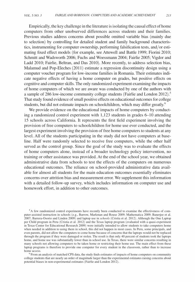
The finding of a zero average treatment effect also does not appear to be due to offsetting effects at the bottom and top of the grade distribution. Figure 1 dis-plays estimates and 95 percent confidence intervals from quantile regressions to test for differential treatment effects across the posttreatment achievement distribution that could be hidden by focusing only on mean impacts (e.g., Bitler, Gelbach, and Hoynes 2006). Estimates of quantile treatment effects are indistinguishable from zero throughout the distribution.23

Overall, the results in this section suggest that computers do not have an impact on grades for students at any point in the distribution. The estimates are robust to focusing on the pass/fail cutoff and quantile treatment effects. We now turn to examining impacts on test scores.

C. Test scores

Our second main outcome is performance on the STAR program tests. As part of the STAR Program, all California students are required to take standardized tests for English-language arts and math each spring. While grades may be the most likely outcome to change because home computers might help or distract students from turning in homework assignments, test scores focus on the impacts on the amount of information children learned during the school year.

Table 4 reports estimates of treatment effects for STAR scores in English ( columns 1 and 2) and math (columns 3 and 4). The dependent variable in panel A is the score on the test (standardized within the control group, so that the dependent variable has mean 0 and standard deviation 1 among control students), while in panel B it is a

23 The estimates displayed in Figure 3 do not control for baseline covariates. Estimates that control for baseline covariates look similar.

Est

imat

ed tr

eat

men

t effe

ct

0 0.05 0.1 0.15 0.2 0.25 0.3 0.35 0.4 0.45 0.5 0.55 0.6 0.65 0.7 0.75 0.8 0.85 0.9 0.95 1

Percentile

Estimated treatment effect 95 percent CI

Quantile treatment effect for posttreatment grade average1

0.8

0.6

0.4

0.2

0

–0.2

–0.4

–0.6

–0.8

–1

Figure 1. Quantile Treatment Effects (Grades)

notes: Dependent variable is the average grade in posttreatment quarters (the third and fourth quarter) in academic subjects (math, science, social studies, English, and computers).

224 AmericAn economic JournAl: Applied economics July 2013

dummy for whether the student is proficient or advanced (getting a 4 or 5 out of 5 on the test). Proficiency and advanced scores meet state standards and are important for schools to satisfy Adequate Yearly Progress (AYP) as part of the No Child Left Behind Act. In columns 1 and 3 of both panels, we include the same controls as in the previous tables. In columns 2 and 4, we also include STAR scores from the previous school year.

From panel A, we find no evidence of an effect of home computers on test scores (with or without controlling for the previous year’s test score). The point estimates are small and very close to zero in all specifications. Focusing on whether students meet proficiency standards in panel B, we also find no evidence of home computer effects on STAR scores. The treatment effect point estimates are zero or very close to zero. Confidence intervals around these point estimates are tight. For English, the 95 percent confidence interval is −0.15 to 0.05 standard deviations for the standard-ized score and −0.04 to 0.04 for the proficiency indicator. For math, the 95 percent confidence intervals are −0.16 to 0.04 standard deviations and −0.08 to 0.04 for the standardized score and proficiency indicator, respectively.

Figure 2 examines the distribution of test scores. Since the STAR scores are lumped into only five bins, we cannot estimate quantile treatment effects. Figure 2 therefore instead plots inverse cumulative distribution functions (CDFs) for both STAR scores, for the treatment and control groups. The CDFs have substantial overlap between the treatment and control groups for both test scores. We find very

Table 4—California STAR Test

English/language arts Math

(1) (2) (3) (4)panel A. standardized scoreTreatment −0.05 −0.05 −0.07 −0.06

(0.06) (0.05) (0.06) (0.05)Prior year’s test score 0.69 0.62

(0.03)*** (0.03)***

Observations 961 961 914 914Control mean 0.00 0.00 0.00 0.00Control SD 1.00 1.00 1.00 1.00

panel B. indicator for proficiency1

Treatment 0.00 0.00 −0.02 −0.02(0.03) (0.02) (0.03) (0.03)

Prior year’s test score 0.25 0.26 (0.01)*** (0.01)***

Observations 961 961 914 914Control mean 0.29 0.29 0.30 0.30Control SD 0.46 0.46 0.46 0.46

notes: Test scores are normalized to have mean 0 and standard deviation 1. See the notes to Table 2 for the list of controls. Regressions also control for the sampling strata (school × year). To avoid dropping observations, for each control variable (including the prior year’s test score), we create a dummy equal to 1 if the variable is missing for a student and code the original variable as a 0 (so that the coefficients are identified from those with nonmissing values).

1 This variable is coded as 1 if the student receives a 4 or 5 (out of 5) on the test, and 0 otherwise.



small ranges over which the distributions do not perfectly overlap suggesting that there are essentially no differential treatment effects at any part of the test score dis-tribution. Thus, mean impact estimates do not appear to be hiding offsetting effects at different parts of the distribution.

D. Other Educational Outcomes

The schools participating in the study provided us with a rich set of additional educational outcomes. From administrative data we examine total credits earned by the end of the third and fourth quarters, the number of unexcused absences, the number of tardies, and whether the student was still enrolled in the school at the end of the year. These measures of educational outcomes complement the results for grades and test scores.

End

line

ST

AR

sco

re (

mat

h)

0 0.2 0.4 0.6 0.8 1

End

line

ST

AR

sco

re (E

nglis

h)

0 0.2 0.4 0.6 0.8 1

Proportion at or below

Treatment

Control

Inverse CDF for endline English STAR score5

4

3

2

1

Panel A. English/language arts

Panel B. Math

5

4

3

2

1

Proportion at or below

Inverse CDF for endline math STAR score

Treatment

Control

Figure 2. Inverse Posttreatment CDFs for STAR Scores

note: Figures depict inverse CDFs for endline STAR scores.


Table 5 reports estimates of treatment effects. Students receiving home comput-ers do not differ from the control group in the total number of credits earned by the end of the third or fourth quarters of the school year. Thus, the home computers are not changing the likelihood that children will be able to move on to the next grade level. Receiving a home computer also does not have an effect on the number of unexcused absences or tardies during the school year, suggesting that it does not alter their motivations about school. Finally, treatment students are no more likely to be enrolled in school at the end of the year than control students. Taken together, these results on additional educational outcomes support the conclusions drawn from the grade and test score results of no effects of home computers.24

E. intermediate inputs and Outcomes from the Follow-up survey

The follow-up survey provides information on several less-commonly measured intermediate educational inputs and outcomes, such as homework effort and time, receiving help on assignments, software use, and computer knowledge. We examine the impact of home computers on these intermediate inputs in Table 6. In panel A, we find no evidence that treatment students spent more time on the last essay or project they had for school. The treatment group is also no more likely to turn their home-work in on time. This latter result is interesting in that reported homework effort is quite low, such that there appears to be scope for improvement—only 47 percent of control students reported that they “always” hand assignments in on time. We also find no difference between treatment and control students in the likelihood that they receive help on school assignments from other students, friends, or teachers by e-mail or networking. Finally, we examine whether having a home computer

24 We also summarize the results for educational outcomes by aggregating the separate measures into a stan-dardized z-score as in Kling, Liebman, and Katz (2007). A regression of a z-score of the main three academic outcomes (grades and the two test scores), including the same set of controls as we have used throughout, yields a coefficient of −0.05 standard deviations with a standard error of 0.05. Also including the 5 main administrative outcomes in Table 5 yields a coefficient of −0.02 standard deviations with a standard error of 0.03.

Table 5—Administrative Outcomes

Total credits in third quarter

Total credits in fourth quarter

Unexcused absences

Number of tardies

Still enrolled at end of year

(1) (2) (3) (4) (5)Treatment 0.04 −0.03 −0.37 −0.21 0.01

(0.09) (0.10) (0.38) (0.93) (0.02)

Observations 1,123 1,123 1,104 1,104 1,123r2 0.40 0.35 0.34 0.24 0.20 Control mean 5.36 5.48 4.94 11.53 0.88Control SD 1.87 1.91 7.84 17.00 0.33

notes: Regressions control for the sampling strata (school × year), and the same list of control as Table 2. The vari-able “Left school by end of year” is coded as a 1 if the student had no grade data in the fourth quarter.



crowds out total time spent doing homework (column 6). High levels of use of home computers for games, social networking, and other forms of entertainment have raised concerns about the displacement of homework time.25 However, we find no evidence that the treatment group reports lower hours of homework time than the control group.

25 These concerns are similar to those over television (Zavodny 2006). There is consistent evidence across many different surveys showing high levels of game, social networking, and other noneducational uses of computers by children (see, for example, Lenhart et al. 2008; Lenhart 2009; Pew Internet Project 2008a, 2008b; US Department of Education 2011a; Kaiser Family Foundation 2010).

Table 6—Effort in School, Software Use, and Computer Knowledge

How much time did you spend on last

How often do you turn in homework on time?

Received help from teacher or classmate

via Internet/

How many hours per

week do you spend on

essay? Always Usually Sometimes e-mail homework?(1) (2) (3) (4) (5) (6) (7)

panel A. self-reported school effortTreatment 0.04 −0.04 0.02 0.01 0.02 −0.08

(0.81) (0.03) (0.03) (0.03) (0.03) (0.27)


panel B. uses a computer for:1

Word processing Research Spreadsheet

Educational software Usage index2

Treatment 0.02 −0.04 0.02 −0.03 −0.01(0.04) (0.03) (0.03) (0.04) (0.02)

Observations 707 707 707 707 707Control mean 0.36 0.75 0.12 0.32 0.39Control SD 0.48 0.43 0.33 0.47 0.26

panel C. Knows how to:Download file from Internet

E-mail a file

Save a report to

hard drive

Save a report to

flash driveCreate a

new folder

Enter a formula in a spreadsheet

Knowledge index2

Treatment 0.03 0.04 −0.04 0.06 0.00 −0.03 0.01(0.04) (0.04) (0.04) (0.04) (0.04) (0.03) (0.02)

Observations 707 707 707 707 707 707 707Control mean 0.49 0.46 0.62 0.55 0.66 0.21 0.50Control SD 0.50 0.50 0.49 0.50 0.48 0.40 0.32

notes: Data is from the follow-up survey completed by students. See the notes to Table 2 for the list of controls.1 The questions in panels B and C were only asked in the second year of the program (2009–2010).2 For both knowledge and usage, the index sums the number of questions for which the student reported “yes” and divides by the total number of questions.



We also asked students what they use computers for and what they know how to do with computers.26 In panel B, we include answers to questions about what types of software students use (including word processing, researching projects or reports, using a spreadsheet, and educational software). Even though baseline usage levels are low for some types of software use, we find no major differences between the treatment and control groups in this dimension. In panel C, we asked students whether they knew how to use a computer for various tasks. Again, baseline knowledge levels are low. For example, 49 percent of students report knowing how to download a file from the Internet, 46 percent report knowing how to e-mail a file, and 62 percent report knowing how to save a file to the hard drive. Despite this, we find no treatment difference in any of these measures. These results for software use and knowledge, and the results for other intermediate educational inputs, are con-sistent with the lack of positive or negative effects for the more ultimate academic outcomes examined above.

III. Treatment Heterogeneity

The results presented thus far provide consistent evidence against the hypothesis that home computers exert a positive or negative effect on academic outcomes at the average and at notable cutoffs in the achievement distribution, such as the pass rate and meeting proficiency standards. In addition, the results from the quantile treatment effect regressions do not provide evidence that home computers shift the achievement distribution at any point in the distribution in a discernible way. In this section, we explore whether there might be heterogeneity in treatment effects by various baseline characteristics. We focus specifically on pretreatment ability, paren-tal supervision, propensity for game/social networking use, and basic demographic characteristics. Focusing on these particular measures is partly motivated by find-ings from the previous literature, and all of these measures were pre-identified at the start of the project (which is why they were asked at baseline).

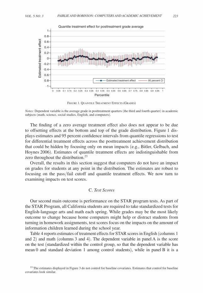
We start by examining heterogeneity by baseline academic achievement. Figure 3 examines treatment effects focusing on potential differences across the pretreatment grade distribution. The graph presents coefficients from the following regression:

(1) yi = β pc × dip × C i + β pt × dip × T i + δ X i + εi .

In the regression, dip is an indicator for whether individual i is in the pth per-centile of the pretreatment GPA distribution. Percentiles are calculated within each school and are restricted to 20 different percentile categories. C i is an indicator for the control group, and T i is an indicator for the treatment group. Thus, β pc and β pt are estimates of the relationship between pre- and posttreatment performance in the control and treatment groups, respectively, and the difference, β pt − β pc provides an estimate of the treatment effect at the pth percentile. X i is a minimal set of controls,

26 These questions were loosely based on the CPS Computer and Internet Supplement, the Microsoft Digital Literacy Test, and Hargittai (2005).


including only subject and quarter indicators (so that the coefficients represent the unconditional relationship between pre- and post-performance for the treatment and control groups). Standard errors are clustered at the individual level, and the 95 per-cent confidence interval of the difference between the treatment and control groups is plotted.

The estimates displayed in the figure indicate that treatment effects are indistin-guishable from zero at almost all points of the pretreatment grade distribution.27 Similarly, Figure 4 examines the effects of home computers on STAR scores by prior achievement levels. Again, there is no discernible effect at almost any point in the pretreatment STAR distribution. These figures suggest minimal effects of com-puters across the pretreatment ability distribution and rule out the possibility that the null estimates of average treatment effects are due to offsetting positive and negative treatment effects at different parts of the pretreatment achievement distribution.

The null effects found above might instead be due to positive effects of home computers on educational outcomes simply offsetting the negative effects from non-educational uses. Computers might be particularly harmful to students who have a high propensity to use them for noneducational purposes (either because their parents do not monitor them closely or because the children are intrinsically more inclined to use them for entertainment).

To explore this question, we first examine whether there is heterogeneity in treatment effects based on parental supervision. In their study of Romanian

27 Appendix Table A3 shows these results in a regression framework as well as treatment interactions with pretreatment levels.

0

0.5

1

1.5

2

2.5

3

3.5

4

Pos

ttrea

tmen

t gra

de

0.05 0.15 0.25 0.35 0.45 0.55 0.65 0.75 0.85 0.95

Percentile in pretreatment grade distribution

Posttreatment grades by pretreatment GPA percentile

Control95 percent CI of differenceTreatment

Figure 3. Posttreatment Grades by Pretreatment GPA Percentile (Quarter 1)

notes: The graph shows estimated coefficients from a regression of posttreatment (quarters three and four) grades on interactions between treatment and pretreatment GPA percentile (in quarter one, before the computers were given out). The vertical line is a 95 percent confidence interval for the difference between the treatment and control groups, at each percentile. The percentiles are calculated within each school. Regressions restricted to “academic subjects” (math, science, English, social studies, and computers). Regressions control for the subject and whether the class was taken in quarter three. There are 1,035 students and 7,202 observations in this regression.


schoolchildren, Malamud and Pop-Eleches (2011) find evidence that parental super-vision through rules on homework activities attenuates some of the negative effects of home computers on grades that they find in the main specifications.28 In designing the baseline survey we asked questions about having rules over how much TV they can watch and whether they have a curfew to measure parental supervision.29 Table 7

28 Malamud and Pop-Eleches (2011) also examine interactions with parental rules regarding computer use, but do not find evidence that they mitigate the negative effects of home computers on school grades. One concern that they note in the paper is that information on parental rules for homework activities and computer use are gleaned from a survey after the children received computers, making these rules potentially endogenous.

29 We also collected information on whether the child usually eats dinner with his/her parents. We find similar results as those for TV rules and having a curfew.

End

line

ST

AR

sco

re

Endline STAR score by pretreatment STAR score percentile

Endline STAR score by pretreatment STAR score percentile

5

4.5

4

3.5

3

2.5

2

1.5

1

0.5

0

0.05 0.15 0.25 0.35 0.45 0.55 0.65 0.75 0.85 0.95

Percentile in pretreatment STAR score distribution


0.05 0.15 0.25 0.35 0.45 0.55 0.65 0.75 0.85 0.95

Percentile in pretreatment STAR score distribution

End

line

ST

AR

sco

re

5

4.5

4

3.5

3

2.5

2

1.5

1

0.5

0


Panel A. English/language arts

Panel B. Math

Figure 4. Posttreatment STAR Scores by Pretreatment Star Percentiles

notes: The graph shows estimated coefficients from a regression of endline STAR scores on interactions between treatment and pretreatment STAR scores. The vertical line is a 95 percent confidence interval for the difference between the treatment and control groups, at each percentile. The percentiles are calculated within each school. There are 865 students in panel A and 790 in panel B.


reports estimates of heterogeneous treatment effects for these two variables. We find that treatment students with curfews increase game use less than other students. However, this difference is evidently too small to have any meaningful impact on outcomes we do not find a relative increase in time devoted to doing homework, grades, or test scores. We also find no evidence suggesting that children with rules for watching TV benefited more or less from home computers.

Computers might be harmful to students who have a high propensity to use them for noneducational purposes. Although this is difficult to measure, we included questions on video game use (e.g., Wii, Xbox) and having a social networking page

Table 7—Heterogeneity by Baseline Measures of Parental Oversight

Weekly hours computer use

Weekly hours computer

use on video games

and social networking

Hours per week spent on

homework

Grades in academic subjects1

Standardized STAR score

English Math

(1) (2) (3) (4) (5) (6)

panel A. TV rules Treatment 2.96 2.28 -0.10 0.02 −0.06 0.05 (0.95)*** (0.65)*** (0.55) (0.09) (0.09) (0.10)Parents have rules for TV −0.28 -0.12 0.30 0.02 −0.03 0.02 at baseline (0.83) (0.56) (0.47) (0.08) (0.08) (0.09)Parents have TV rules at baseline −0.65 −1.21 0.03 0.01 0.01 −0.15 × treatment (1.09) (0.75) (0.63) (0.10) (0.11) (0.12)p-value for interaction + main treatment effect

0.01*** 0.01*** 0.82 0.57 0.38 0.11

Mean of interacted variable 0.75 0.74 0.75 0.75 0.75 0.75

Observations 755 671 825 7,820 961 914Number of students 755 671 825 1,035 961 914Control mean of dependent variable 4.23 1.41 2.64 2.26 0.00 0.00Control SD 5.22 3.01 3.52 1.36 1.00 1.00

panel B. Curfew Treatment 4.02 2.85 −0.28 −0.02 −0.15 −0.22 (1.10)*** (0.73)*** (0.64) (0.10) (0.11) (0.12)*Has curfew at baseline 0.08 −0.08 −0.74 −0.08 −0.08 0.02 (0.95) (0.64) (0.55) (0.09) (0.09) (0.10)Has curfew at baseline × treatment −1.60 −1.67 0.28 0.05 0.13 0.17 (1.22) (0.81)** (0.72) (0.11) (0.12) (0.14)p-value for interaction + main treatment effect

0.01*** 0.01*** 1.00 0.56 0.62 0.38


Observations 723 641 788 7,501 926 880Number of students 723 641 788 991 926 880Control mean of dependent variable 4.03 1.29 2.68 2.25 0.01 0.01Control SD 4.20 2.12 3.56 1.35 1.00 1.00

notes: All regressions include controls for the sampling strata (school × year) and the same controls as in Table 2. GPA and test score regressions control for the pretreatment level of the given variable. Mean and median reported baseline video game playing are 1.8 and 1 hours per week.

1 Course are restricted to “academic subjects” (math, English, social studies, science, and computers).*** Significant at the 1 percent level. ** Significant at the 5 percent level. * Significant at the 10 percent level.


on the baseline survey. These measures are clearly not perfect because families that have a video game console or children who have a social networking page, but do not have a computer at home, might differ along many dimensions. But, both base-line measures are exogenous to treatment and provide some suggestive evidence on the question. Table 8 reports estimates of heterogeneous treatment effects by these two measures. The estimates generally show no differential effects of home computers on outcomes by whether students have a propensity to use computers for noneducational purposes. The one somewhat surprising result is that we find a negative level effect of having a social networking page, but a positive interaction

Table 8—Heterogeneity by Baseline Propensity to Use Computers for Noneducational Purposes

Weekly hours computer use

Weekly hours computer

use on video games

and social networking

Hours per week spent on

homework



English Math

(1) (2) (3) (4) (5) (6)panel A. Has social networking pageTreatment 2.19 1.24 −0.38 −0.04 −0.08 −0.09

(0.61)*** (0.42)*** (0.35) (0.05) (0.06) (0.07)Has social networking page −0.55 0.19 −0.54 −0.30 −0.04 −0.09 at baseline (0.73) (0.51) (0.42) (0.07)*** (0.07) (0.08)Has social networking page 1.12 0.47 0.85 0.21 0.08 0.08 at baseline × treatment (1.00) (0.69) (0.57) (0.09)** (0.10) (0.11)p-value for interaction + main treatment effect

0.01*** 0.01*** 0.30 0.03** 1.00 0.91


Observations 743 660 813 7,729 951 905Number of students 743 660 813 1,023 951 905Control mean of dependent variable

4.17 1.39 2.67 2.25 0.01 0.01

Control SD 5.05 2.97 3.54 1.36 1.00 1.00

panel B. Video game playingTreatment 2.66 1.61 −0.46 −0.03 −0.07 −0.04

(0.79)*** (0.55)*** (0.45) (0.07) (0.07) (0.08)Played video games at baseline 1.18 0.47 0.24 −0.13 −0.02 −0.03

(0.71)* (0.49) (0.41) (0.06)** (0.07) (0.08)Played video games at baseline −0.12 −0.26 0.59 0.10 0.02 −0.05 × treatment (1.00) (0.69) (0.57) (0.09) (0.10) (0.11)p-value for interaction + main treatment effect

0.01*** 0.01*** 0.70 0.27 0.45 0.15


Observations 742 660 810 7,663 944 897Number of students 742 660 810 1,014 944 897Control mean 4.15 1.35 2.65 2.26 0.01 0.02Control SD 5.04 2.90 3.54 1.36 1.00 1.00

notes: All regressions include controls for the sampling strata (school × year) and the same controls as in Table 2. GPA and test score regressions control for the pretreatment level of the given variable. Mean and median reported baseline video game playing are 1.8 and 1 hours per week.

1 Course are restricted to “academic subjects” (math, English, social studies, science, and computers).*** Significant at the 1 percent level. ** Significant at the 5 percent level. * Significant at the 10 percent level.


effect in the grade regression. One possible interpretation of this result is that play-ing on a computer at home is less of a distraction than going to a friend’s house to use a computer, though since this is the only significant result it may well be due to sampling variation. Otherwise, we find no heterogeneity along these dimensions.30

We also examine how impacts vary with a few standard demographic background characteristics: gender, race, and grade in school.31 Appendix Table A4 reports esti-mates. We find no evidence of differential treatment effects. Although we do not find evidence of heterogeneity in impacts across these groups for the sample of children that do not have computers in the first place, it is important to note that we cannot necessarily infer that there is no heterogeneity in computer impacts across demographic groups for the broader population of schoolchildren. One issue that is especially salient for the comparison by minority status is that we are likely sam-pling from a different part of the distribution of overall minority students than non-minority students when we focus on noncomputer owners (because of substantially lower rates of ownership among minorities even conditioning on income). But, these results do tell us whether there are differential benefits from home computers among schoolchildren that do not currently own computers, which is clearly relevant for policies to expand access to home computers.32

IV. Conclusion

Even today, roughly one out of every four children in the United States does not have a computer with Internet access at home (NTIA 2011). While this gap in access to home computers seems troubling, there is no theoretical or empirical consensus on whether the home computer is a valuable input in the educational production function and whether these disparities limit academic achievement. Prior studies show both large positive and negative impacts. We provide direct evidence on this question by performing an experiment in which 1,123 schoolchildren in grades 6–10, across 15 different schools and five school districts in California were randomly given comput-ers to use at home. By only allowing children without computers to participate, placing no restrictions on what they could do with the computers, and obtaining administrative data with virtually no attrition and measurement error, the experiment was designed to improve the likelihood of detecting effects, either positive or negative.

30 Another reason that use of computers for entertainment might not affect academic outcomes is that very few students report substantial amounts of game and social networking use on the computer on the follow-up survey. Less than 6 percent of the treatment group reports using their home computers for games and social networking 10 or more hours per week. Another interesting finding from examining the joint distribution of schoolwork use and game/networking use is that most students did both, instead of there being a clear distinction between educational and game/social networking users.

31 Previous survey evidence indicates that, on average, boys and girls use computers differently. Boys tend to use computers more for video games, while girls tend to use them more for social networking (Pew Internet Project 2008a, b; US Department of Education 2011a; Kaiser Family Foundation 2010). Treatment effects may differ by race because of varying rates of access to personal computers at alternative locations, such as at friends’ and rela-tives’ houses, and libraries, and social interactions with other computer users (Fairlie 2004; Goldfarb and Prince 2008; Ono and Zavodny 2007; NTIA 2011). Effects might also differ by grade because of curricular differences.

32 We also test for social interactions in usage. To do this, we interact treatment with the percent of students with home computers in each school (based on results of our in-class survey reported in Appendix Table A1). We find no evidence of social interactions, which may be due to only having variation across schools and not students for this variable.


Although the experiment substantially increased computer ownership and usage without causing substitution away from use at school or other locations outside the home, we find no evidence that home computers had an effect (either positive or nega-tive) on any educational outcome, including grades, standardized test scores, or a host of other outcomes. Our estimates are precise enough to rule out even modestly-sized positive or negative impacts. We do not find effects at notable points in the distribu-tion, such as pass rates and meeting proficiency standards, throughout the distribution of posttreatment outcomes, throughout the distribution of pretreatment achievement, or for subgroups pre-identified as potentially more likely to benefit.

These findings are consistent with a detailed analysis of time use on the com-puter and “intermediate” inputs in education. We find that home computers increase total use of computers for schoolwork, but also increase total use of computers for games, social networking, and other entertainment, which might offset each other. We also find no evidence of positive effects on additional inputs, such as turning assignments in on time, time spent on essays, getting help on assignments, software use, and computer knowledge. On the other hand, we also find no evidence of a dis-placement of homework time. Game and social networking use might not have been extensive enough, within reasonable levels set by parents or interest by children, to negatively affect homework time, grades, and test scores. The potential negative effects of computers for US schoolchildren might also be much lower than the large negative effects on homework time and grades found for Romanian schoolchildren in Malamud and Pop-Eleches (2011), where most households do not have a com-puter at home, because there is less of a novelty of home computers for low-income schoolchildren in the United States for game use. Computers are also used much more extensively in US schools, which might exert more of a positive offsetting effect. Thus, for US schoolchildren, and perhaps schoolchildren from other devel-oped countries, concerns over the negative educational effects of computer use for games, social networking, and other forms of entertainment may be overstated.

An important caveat to our results is that there might be other effects of having a computer that are not captured in measurable academic outcomes. For example, com-puters may be useful for finding information about colleges, jobs, health and consumer products, and may be important for doing well later in higher education. It might also be useful for communicating with teachers and schools and parental supervision of stu-dent performance through student information system software.33 A better understand-ing of these potential benefits is important for future research.

Nevertheless, our results indicate that computer ownership alone is unlikely to have much of an impact on short-term schooling outcomes for low-income children. Existing and proposed interventions to reduce the remaining digital divide in the United States and other countries, such as large-scale voucher programs, tax breaks for educational purchases of computers, Individual Development Accounts (IDAs),

33 Student information system software that provides parents with nearly instantaneous information on their chil-dren’s school performance, attendance and disciplinary actions is becoming increasingly popular in US schools (e.g., School Loop, Zangle, ParentConnect, and Aspen). We find evidence from the follow-up survey of a positive effect of home computers on whether parents check assignments, grades and attendance online using these types of software.


and one-to-one laptop programs, need to be realistic about their potential to reduce the current achievement gap.34

Appendix

34 In the United States, in addition to one-to-one laptop programs, the American Recovery and Reinvestment Act of 2009 provides tax breaks for education-related purchases of computers, and there are many local IDAs in the United States that provide matching funds for education-related purchases of computers. England recently pro-vided free computers to nearly 300,000 low-income families with children at a total cost of £194 million through the Home Access Programme. Another example is the Romanian Euro 200 program which provides vouchers to low-income families with children to purchase computers.

Table A2—Attrition

Appears in baseline

adminstrative dataset

Appears in follow-up

administrative dataset

Appears in grade dataset

(1) (2) (3) (4)

panel A. Administrative outcomesTreatment 0.00 0.00 −0.01

(0.01) (0.01) (0.01)

Observations 1,123 1,123 1,123Sample Full Full FullControl mean 0.99 0.99 0.99

Has STAR scores

Returned follow-up survey

Has STAR scores

Returned follow-up survey

panel B. Test scores and follow-up surveyTreatment 0.01 0.02 −0.01 0.00

(0.02) (0.02) (0.01) (0.02)

Observations 1,123 1,123 992 992Sample Full Full Restricted to those

still enrolled at end of yearControl mean 0.87 0.76 0.96 0.84

notes: Regressions restricted to those students who enrolled in the program at baseline (those who completed a baseline survey and a consent form).


Table A1—Computer Ownership and Participation Rates

Number of students completing in-class survey 7,337

Of those completing survey: Number of students without a computer 1,636 Percentage1 0.24

Of those without a computer: Number of students returning baseline survey 1,123 Percentage 0.67

1 Percentages (columns 3 and 5) exclude one school that did not provide figures on the total number of eligible children.


Table A3—Heterogeneity by Pretreatment Performance



English Math

(1) (2) (3) (4) (5) (6)Treatment 0.03 0.15 −0.06 −0.12 −0.10 −0.07

(0.10) (0.10) (0.05) (0.08) (0.05)* (0.09)LevelsQuarter 1 GPA in academic subjects −0.01 × treatment (0.04)Quarter 1 GPA in academic subjects 0.70

(0.03)***

Standardized pretreatment STAR 0.01 score (English) × treatment (0.05)Standardized pretreatment STAR 0.69 score (English) (0.03)***

Standardized pretreatment STAR −0.05 score (Math) × treatment (0.05)Standardized pretreatment STAR 0.65 score (Math) (0.04)***

Quartiles2

In second quartile at baseline −0.27 0.04 0.02 × treatment (0.14)* (0.11) (0.13)In third quartile at baseline −0.30 0.12 0.00 × treatment (0.13)** (0.13) (0.01)In fourth quartile at baseline 0.02 0.08 −0.10 × treatment (0.13) (0.21) (0.13)In second quartile at baseline 0.79 0.86 0.79

(0.10)*** (0.08)*** (0.09)***

In third quartile at baseline 1.27 1.62 0.00(0.08)*** (0.09)*** (0.01)

In fourth quartile at baseline 1.91 2.12 1.53(0.09)*** (0.16)*** (0.10)***

Observations 7,795 7,795 865 865 790 790Number of students 1,032 1,032 865 865 790 790r2 0.37 0.36 0.58 0.58 0.48 0.46Control mean 2.26 2.26 0.05 0.05 0.07 0.07Control SD 1.35 1.35 1.00 1.00 0.99 0.99

notes: All regressions include controls for the sampling strata (school × year) and the same controls as in Table 2.1 “Academic subjects” include math, English, social studies, science, and computers.2 The quartiles are for the pretreatment levels of the dependent variables (quarter 1 GPA in columns1–2, pretreatment English STAR score in columns 3–4, and pretreatment Math STAR score in columns 5–6).



Table A4A—Heterogeneity by Demographic Characteristics (Grades)


(1) (2) (3)Treatment 0.17 0.01 0.00

(0.09)* (0.06) (0.12)Quarter 1 GPA in academic subjects 0.70 0.70 0.70

(0.02)*** (0.02)*** (0.02)***

Minority student −0.13(0.16)

Minority student × treatment −0.17(0.11)*

Female 0.12(0.06)*

Female × treatment 0.04(0.09)

Grade 7 1.12(0.54)**

Grade 7 × treatment 0.01(0.14)

Grade 8 1.17(0.53)**

Grade 8 × treatment 0.04(0.14)

p-value for interaction + main treatment effect 0.94 0.47 —Mean of interacted variable 0.83 0.50 —

Observations 7,792 7,820 7,820Number of students 1,031 1,035 1,035Control mean 2.25 2.26 2.26Control SD 1.36 1.36 1.36

notes: All regressions include controls for the sampling strata (school × year) and the same controls as in Table 2. In the grade level regressions, the coefficients for high school are included but not shown as there are very few stu-dents in the sample in high school.

1 GPA is in “academic subjects” (math, English, social studies, science, and computers).*** Significant at the 1 percent level. ** Significant at the 5 percent level. * Significant at the 10 percent level.


REFERENCES

Angrist, Joshua, and Victor Lavy. 2002. “New Evidence on Classroom Computers and Pupil Learn-ing.” Economic Journal 112 (482): 735–65.

Attewell, Paul, and Juan Battle. 1999. “Home Computers and School Performance.” information soci-ety 15 (1): 1–10.

Banerjee, Abhijit V., Shawn Cole, Esther Duflo, and Leigh Linden. 2007. “Remedying Education: Evidence from Two Randomized Experiments in India.” Quarterly Journal of Economics 122 (3): 1235–64.

Barrera-Osorio, Felipe, and Leigh L. Linden. 2009. “The Use and Misuse of Computers in Education: Evidence from a Randomized Experiment in Colombia.” World Bank Impact Evaluation Series 29, Policy Research Working Paper 4836.

Barrow, Lisa, Lisa Markman, and Cecelia E. Rouse. 2009. “Technology’s Edge: The Educational Ben-efits of Computer-Aided Instruction.” American Economic Journal: Economic policy 1 (1): 52–74.

Bitler, Marianne P., Jonah B. Gelbach, and Hilary W. Hoynes. 2006. “What Mean Impacts Miss: Dis-tributional Effects of Welfare Reform Experiments.” American Economic review 96 (4): 988–1012.

Table A4B—Heterogeneity by Demographic Characteristics (Test Scores)


English Math

(1) (2) (3) (4) (5) (6)Treatment −0.02 0.00 0.17 −0.12 −0.13 −0.05

(0.11) (0.07) (0.15) (0.12) (0.07)* (0.16)Pretreatment STAR score 0.69 0.69 0.69 (English) (0.03)*** (0.03)*** (0.03)***

Pretreatment STAR score 0.62 0.62 0.62 (math) (0.03)*** (0.03)*** (0.03)***

Minority student 0.00 0.01(0.18) (0.19)

Minority −0.04 0.08 student × treatment (0.12) (0.13)Female 0.14 −0.11

(0.07)** (0.07)Female × treatment −0.10 0.14

(0.09) (0.10)Grade 7 0.04 0.08

(0.14) (0.86)Grade 7 × treatment −0.24 −0.10

(0.16) (0.18)Grade 8 0.15 0.10

(0.16) (0.86)Grade 8 × treatment −0.27 0.06

(0.17) (0.18)p-value for interaction + main treatment effect

0.24 0.13 — 0.43 0.87 —

Mean of interacted variable

0.83 0.51 — 0.83 0.51 —

Observations 958 961 961 913 914 914Number of students 958 961 961 913 914 914Control mean 0.00 0.00 0.00 0.00 0.00 0.00Control SD 1.00 1.00 1.00 1.00 1.00 1.00

note: All regressions include controls for the sampling strata (school × year) and the same controls as in Table 2.*** Significant at the 1 percent level. ** Significant at the 5 percent level. * Significant at the 10 percent level.


California Department of Education. 2010. “2010 STAR Test Results: California STAR Program.” http://star.cde.ca.gov/star2010/ (accessed April 18, 2012).

Carrillo, Paul, Mercedes Onofa, and Juan Ponce. 2010. “Information Technology and Student Achieve-ment: Evidence from a Randomized Experiment in Ecuador.” Inter-American Development Bank Working Paper 223.

Cristia, Julián P., Pablo Ibarrarán, Santiago Cueto, Ana Santiago, and Eugenio Severín. 2012. “Tech-nology and Child Development: Evidence from the One Laptop per Child Program.” Inter-Ameri-can Development Bank Working Paper 304.

Fairlie, Robert W. 2004. “Race and the Digital Divide.” B. E. Journal of Economic Analysis & policy 3 (1): Article 21.

Fairlie, Robert W. 2005. “The Effects of Home Computers on School Enrollment.” Economics of Edu-cation review 24 (5): 533–47.

Fairlie, Robert W., Daniel O. Beltran, and Kuntal K. Das. 2010. “Home Computers and Educational Outcomes: Evidence from the NLSY97 and CPS.” Economic inquiry 48 (3): 771–92.

Fairlie, Robert W., and Rebecca A. London. 2012. “The Effects of Home Computers on Educational Outcomes: Evidence from a Field Experiment with Community College Students.” Economic Jour-nal 122 (561): 727–53.

Fairlie, Robert W., and Jonathan Robinson. 2013. “Experimental Evidence on the Effects of Home Computers on Academic Achievement among Schoolchildren: Dataset.” American Economic Jour-nal: Applied Economics. http://dx.doi.org/10.1257/app.5.3.211.

Fiorini, M. 2010. “The Effect of Home Computer Use on Children’s Cognitive and Non-Cognitive Skills.” Economics of Education review 29 (1): 55–72.

Fuchs, Thomas, and Ludger Woessmann. 2004. “Computers and Student Learning: Bivariate and Mul-tivariate Evidence on the Availability and Use of Computers at Home and at School.” CESifo Work-ing Paper 1321.

Goldfarb, Avi, and Jeff Prince. 2008. “Internet Adoption and Usage Patterns Are Different: Implica-tions for the Digital Divide.” information Economics and policy 20 (1): 2–15.

Goolsbee, Austan, and Jonathan Guryan. 2006. “The Impact of Internet Subsidies in Public Schools.” review of Economics and statistics 88 (2): 336–47.

Hargittai, Eszter. 2005. “Survey Measures of Web-Oriented Digital Literacy.” social science Com-puter review 23 (3): 371–79.

Kaiser Family Foundation. 2010. Generation m2: media in the Lives of 8- to 18-year Olds. Kaiser Family Foundation Study. Washington, DC, January.

Kirkpatrick, Heather, and Larry Cuban. 1998. “Computers Make Kids Smarter—Right?” Technos Quarterly for Education and Technology 7 (2).

Kling, Jeffrey R., Jeffrey B. Liebman, and Lawrence F. Katz. 2007. “Experimental Analysis of Neigh-borhood Effects.” Econometrica 75 (1): 83–119.

Lenhart, Amanda. 2009. “The Democratization of Online Social Networks: A look at the change in demographics of social network users over time.” Paper presented at Pew Internet & American Life Project AoIR 10.0, Milwaukee, October 8.

Lenhart, Amanda, Joseph Kahne, Ellen Middaugh, Alexandra Rankin Macgill, Chris Evans, and Jessica Vitak. 2008. Teens, Video Games, and Civics: Teens’ gaming experiences are diverse and include significant social interaction and civic engagement. Pew Internet and American Life Proj-ect, Washington, DC, September.

Lowther, Deborah L., J. Daniel Strahl, Fethi A. Inan, and Jerry Bates. 2007. Freedom to Learn program: michigan 2005–2006 Evaluation report. Center for Research in Educational Policy, Memphis, March.

Machin, Stephen, Sandra McNally, and Olmo Silva. 2007. “New Technology in Schools: Is There a Payoff?” Economic Journal 117 (522): 1145–67.

Malamud, Ofer, and Cristian Pop-Eleches. 2011. “Home Computer Use and the Development of Human Capital.” Quarterly Journal of Economics 126 (2): 987–1027.

Market Data Retrieval (MDR). 2004. Technology in Education. Shelton, CT: Market Data Retrieval.Mathematica. 2009. Effectiveness of reading and mathematics software products: Findings from Two

student Cohorts. U.S. Department of Education. Jessup, MD.National Telecommunications and Information Administration. 2011. “Current Population Survey

(CPS) Internet Use 2010.” http://www.ntia.doc.gov/data/CPS2010_Tables_.Noll, Roger G., Dina Older-Aguilar, Gregory Rosston, and Richard R. Ross. 2000. “The Digital Divide:

Definitions, Measurement, and Policy Issues.” Paper presented at Bridging the Digital Divide: Cali-fornia Public Affairs Forum, Stanford University, Stanford.

Ono, Hiroshi, and Madeline Zavodny. 2007. “Digital Inequality: A Five Country Comparison Using Microdata.” social science research 36 (3): 1135–55.

http://star.cde.ca.gov/star2010


http://www.ntia.doc.gov/data/CPS2010_Tables_


Pew Internet Project. 2008. Writing, Technology and Teens. Pew Internet & American Life Project. Washington, DC, April.

Pew Internet Project. 2008. Teens, Video Games, and Civics. Washington, DC: Pew Internet & Ameri-can Life Project.

Rivkin, Steven G., Eric A. Hanushek, and John F. Kain. 2005. “Teachers, Schools, and Academic Achievement.” Econometrica 73 (2): 417–58.

Schmitt, John, and Jonathan Wadsworth. 2006. “Is There an Impact of Household Computer Own-ership on Children’s Educational Attainment in Britain?” Economics of Education review 25 (6): 659–73.

Shapley, Kelly, Daniel Sheehan, Catherine Maloney, and Fanny Caranikas-Walker. 2009. Evaluation of the Texas Technology immersion pilot: Final Outcomes for a Four-year study (2004-05 to 2007-08). Texas Center for Educational Research. Austin.

Silvernail, David L., Caroline A. Pinkham, Sarah E. Wintle, Leanne C. Walker, and Courtney L. Bartlett. 2011. A middle school One-to-One Laptop program: The maine Experience. Maine Edu-cation Policy Research Institute, University of Southern Maine, Gorham, ME, August.

Universal Service Administration Company. 2010. 2010 Annual report. http://www.usac.org/about/tools/publications/annual-reports/2010/index.html.

U.S. Department of Education. 2011a. digest of Education statistics 2010 (nCEs 2011-015). National Center for Education Statistics, Institute of Education Sciences, U.S. Department of Education. Washington, DC, April.

U.S. Department of Education. 2011b. “School Locator.” National Center for Educational Statistics. http://nces.ed.gov/ccd/schoolsearch/ (accessed April 18, 2012).

Vigdor, Jacob L., and Helen F. Ladd. 2010. “Scaling the Digital Divide: Home Computer Technology and Student Achievement.” National Bureau of Economic Research (NBER) Working Paper 16078.

Zavodny, Madeline. 2006. “Does Watching Television Rot Your Mind? Estimates of the Effect on Test Scores.” Economics of Education review 25 (5): 565–73.

http://www.usac.org/about/tools/publications/annual-reports/2010/index.html

http://www.usac.org/about/tools/publications/annual-reports/2010/index.html

http://nces.ed.gov/ccd/schoolsearch

experimental evidence on the effects of home computers on

Documents