experimental investigation high entrainment jet pumps · · 2013-08-31experimental investigation...

N A S A C O N T R A C T O R R E P O R T

ANALYTICAL AND EXPERIMENTAL INVESTIGATION OF HIGH ENTRAINMENT JET PUMPS

by Kenneth E. Hickman, Gerald B. Gilbert, und John H. Carey

Prepared by DYNATECH R/D COMPANY

Cambridge, Mass. for Ames Research Cetzter

N A T I O N A L A E R O N A U T I C S A N D S P A C E A D M I N I S T R A T I O N W A S H I N G T O N , D . C. J U L Y 1970

https://ntrs.nasa.gov/search.jsp?R=19700024692 2018-07-02T10:53:32+00:00Z

ANALYTICAL AND EXPERIMENTAL INVESTIGATION

OF’ H I G H E N T R A I N M E N T J E T P U M P S

By Kenneth E. H i c k m a n , G e r a l d B. G i l b e r t , a n d John H . C a r e y

, . 7

for A m e s R e s e a r c h C e n t e r

NATIONAL AERONAUTICS AND SPACE ADMINISTRATION

F o r s a l e by t h e C l e o r i n g h o u s e f o r F e d e r a l S c i e n t i f i c a n d T e c h n i c 0 1 I n f o r m a t i o n S p r i n g f i e l d , V i r g i n i a 22151 - CFSTI p r i c e $3.00

TABLEOFCONTENTS

Section

1

2

3

4

SUMMARY

INTRODUCTION

1.1 Background 1.2 Previous Work 1.3 Purpose

SYMBOLS

2 . 1 Symbols Used in the Analysis and Test Results 2.2 Symbols Used in the Computer Program

ANALYSIS

3. 1 Formulation of the Mathematical Model

3. 1.1 Assumptions Used in the Analysis 3. 1 .2 Analysis of the Accommodation Region 3. 1.3 Analysis of the Mixing Region 3.1.4 Jet Pump Performance Parameters 3.1.5 Inclusion of Mixing Tube Wall Friction 3. 1.6 Dimensionless Formulation 3. 1.7 Maximum Entrainment Ratio

3.2 The Computer Program

3.3 Solutions for a Range of Jet Pump Designs 3.4 Jet PumpDuct Matching Considerations

Page

2

2 3 5

6

6 9

12

12

13 13 16 18 19 22 28

28

29 31

3 . 4 . 1 3 .4 .2 3.4.3 3.4.4

3 .4 .5 3.4. 6

3.4.7

3.4.8

Representation of Duct Loss Characteristics 31 Evaluation of the Loss Coefficient, K 32 Development of System Performance kquations 33 Calculation Procedure for Determining the Operating Point of a Jet Pump in a Duct System 38 Sample Calculation 40 Influence of Blowing Duct Area Ratio and Duct Losses Upon Entrainment 42 Influence of Blowing Duct Area Ratio and Duct Losses Upon Thrust Augmentation 44 Conclusions 45

TEST PROGRAM 47

4.1 Test Arrangement 47 4.2 Instrumentation and Data Reduction Procedures 50

ii

TABLE OF CONTENTS (Continued)

Section

4. 2.1 Instrumentation 4.2.2 Data Reduction Procedures 4.2.3 Suction Duct and Nozzle Cluster Losses 4 .2 .4 Pressure Loss Due to Wall Friction in the

Constant-Area Mixing Tube

4.3 Tabulation of Test Conditions

4.3. 1 Presentation of Data

4.4 Discussion of Test Results

4.4.1 Comparison of Constant-Area and NAS 2-2518 Varying-Area Mixing Tubes

4.4.2 Reduced Blockage Nozzle Clusters 4.4.3 Comparison of Short and Extended Mixing Tubes 4.4.4 Velocity Profile Investigations

5 COMPARISON OF ANALYTICAL AND EXPERIMENTAL RESULTS

5. 1 Jet Pump Stagnation Pressure Rise 5 . 2 Jet Pump Static Pressure Rise

6 CONCLUSIONS

APPENDIX A - Listing of the Computer Program

APPENDIX B Discussion of the Computer Program by Blocks

APPENDIX C - Typical Computer Solutions

REFERENCES

TABLES

Page

50 51 53

56

57

58

58

58

63 6G 71

74

74 76

78

81

90 98

107

110

FIGURES 129

iii

ANALYTICAL AND EXPERIMENTAL INVESTIGATION OF HIGH ENTRAINMENT J E T PUMPS

by Kenneth E. Hickman, Gerald B. Gilbert, and John H. Carey

SUMMARY

The use of jet pumps is of increasing interest for boundary layer control

or control force augmentation in V/STOL aircraft . In typical applications, a small mass flow of p r imary a i r a t p re s su res up to 400 psia can be used to entrain a much l a rge r mass flow of secondary air at ambient conditions. The primary nozzle flow

is supersonic while the secondary flow is subsonic. The jet pump system design ob-

jectives may be maximum entrainment, maximum thrust augmentation, or some combination of the two. Little information is available in the l i terature to guide the

designer of jet pumps for such applications.

In this investigation, a simple analytical model was developed to predict the performance of high-entrainment compressible flow jet pumps with constant area

mixing tubes. While the model is suitable for hand calculation, a computer program

was prepared to facilitate calculation of jet pump performance curves and allow com-

parison of different jet pump designs. Analytical techniques were developed for

matching the jet pump design to its associated duct system in order to achieve maximum entrainment or thrust augmentation.

The validity of the analytical model was confirmed by an extensive test program using a multiple-nozzle jet pump with two different mixing tube lengths.

The primary-to-secondary flow area ratios were varied from 0.0013 to 0.0067.

The primary flow pressure ranged from 55 psia to 350 psia.and the pr imary flow temperature ranged from 200" F to 1200" F. The observed entrainment ratios varied

from 15 to 37. The performance of each jet pump geometry was measured over a

very broad range of operating conditions in order to develop performance maps for comparison with the analytical predictions.

Section 1

INTRODUCTION

1.1 Background

Jet pumps have been used for many years in industrial applications where

a high-pressure gas such as steam is used to pump a lower-pressure gas. The jet pump i s a simple low-cost device with no moving parts and is particularly convenient

for use with troublesome fluids such as two-phase flows, high-temperature gases, or corrosive gases. Jet pumps are usually employed as low-pressure-rise devices

and their thermodynamic efficiency is low, i. e . , under 20%. Because they are low-

cost devices of limited performance potential, there has not been a strong incentive

for research and development work on industrial jet pumps.

In recent years, applications of jet pumps to boundary layer control sys-

tems have become of increasing interest for STOL aircraft. Systems have been pro-

posed which use jet pumps to entrain a large flow of secondary air which is then

directed over a deflected flap for lift augmentation. In a configuration patented by

F. G. Wagner (references 1 and 2 ) , a jet pump is used to entrain air from one sec-

tion of the trailing edge of a wing (boundary layer suction upstream of a deflected

flap) and then to discharge it over a deflected flap. In this way, the inherent ineffi-

ciency of the jet pump is partially balanced by the double employment of the entrained

air for boundary layer control. Jet pumps may also have application in VTOL a i r -

craft for direct lift o r control force augmentation. The primary, high-pressure flow

for the jet pumps can be provided by a bleed from the main engine compressors o r by

an auxiliary power unit.

The use of jet pumps as primary components of V/STOL aircraf t sys -

tems places new emphasis upon development of design techniques for these devices.

It is essential to be able to minimize the size of jet pumps for particular primary

and secondary flow conditions, and to be able to predict the performance of jet pumps

over a broad range of operating conditions. However, systematic design and analy-

s i s p rocedures a re not available for high-entrainment-ratio compressible-flow jet

pumps.

2

1 . 2 Previous Work

A number of investigators have carried out analytical and experimental

studies of a i r - to-air je t pumps, p~imari ly for appl icat ions requir ing high pressure

rise or thrust augmentation. ThG entrainment ratios developed by these jet pumps

are low, generally less than 10. Thus, this work is not directly applicable to the

high entrainment requirements of V/STOL aircraft systems. Nevertheless, this

work provides useful guidance for the development of performance prediction tech-

niques and design rules for high-entrainment jet pumps. A brief review of some of the principal air-to-air jet pump papers follows.

The performance of constant-area jet pumps was analyzed by McClintock

and Hood for a range of design and operating conditions in reference 3. The analy-

sis was prepared by assuming incompressible flow but the influence of compressi-

bility was discussed in qualitative terms. Empirical coefficients derived by testing

were included in the theory. The influence of mixing length and the use of various multiple-nozzle primary flow geometries were studied experimentally. The jet

pumps treated had entrainment ratios of 10 or less; the design goal for the study was

achievement of maximum thrust augmentation.

A one-dimensional method of analysis of jet pumps was developed by

Keenan, Neumann , and Lustwerk in reference 4. The analysis was applied to both

constant-area and constant-pressure mixing processes. Test results were obtained for jet pumps with secondary-to-primary area ratios up to 100, primary-to-secondary

pressure ratios up to 200, and a primary-to-secondary temperature ratio of 1 .0 .

The various regimes of operation of jet pumps with supersonic primary flows and

both supersonic and subsonic primary flows were described. The analytical results given were for jet pumps developing substantial stagnation pressure rises

(e. g. , pressure ra t ios f rom 2 to 10) a t low entrainment ratios (under 10).

Fabri carr ied out a number of experiments on jet pumps which supple-

ment the results reported by Keenan, et al. Fabri 's results, with supporting analy-

sis, a r e given in references 5 and 6. These tests also were confined to low entrainment ratio jet pumps. Excellent agreement was obtained between analytical predic-

tions and measured jet pump performance.

3

An extensive analytical and experimental program was conducted at the

University of Minnesota Rosemount Aeronautical Laboratories on jet pumps with

secondary-to-primary area ratios up to 36, primary-to-secondary pressure ratios

up to 32, and primary-to-secondary temperature ratios up to 3.3. The results are presented in references 7 , 8, and 9. Single-nozzle primary flows with constant-

area mixing tubes were used in these studies. High entrainment ratios were not an

objective of the jet pump design; typical entrainment ratios reported were less than

3. A number of analytical results showing the influence of duct matching upon jet

pump and system performance were included in the reports.

An analytical procedure for constant-area jet pumps with subsonic pri-

m a r y flow was developed in reference 10. A computer program was prepared for

use in optimizing jet pump design for particular application requirements. An analy-

sis applicable to supersonic primary flows is given in reference 11. The analysis

was compared with test results, but was not otherwise applied for jet pump design or

optimization.

The performance of a high-entrainment jet pump was measured in the

Wagner "Jet Induced Lift" boundary layer control system (figure 1 ). These tests

were performed by the present investigators under NASA contract No. NAS2-2518.

The resul ts are reported in reference 12. The jet pump component of the system

employed a variable-area mixing tube (designed in an effort to obtain constant pres-

s u r e mixing) and a 9-nozzle cluster for the primary flow. The jet pump was tested

in the system at secondary-to-primary area ratios ranging from 150 to 800, primary-

to-secondary pressure ratios up to 26, and primary-to-secondary temperature ratios

up to 5.5. The desired constant pressure distribution in the mixing tube was not

achieved. The entrainment ratios predicted for the complete sys temwere notattained.

The results of the NAS2-2518 program showed that the methods used to design the

high-entrainment jet pump and to match it to the duct flow characterist ics were in-

adequate. These results provided the impetus for the present study.

4

1 . 3 Purpose

The objectives of this investigation were as follows:

0 to develop analytical procedures for predicting the

performance of high-entrainment-ratio jet pumps

0 to demonstrate the application of these procedures

to match a jet pump design to its connecting duct

s y s tem

0 to verify the analytical procedures by testing a jet pump over a broad range of operating conditions and

jet pump geometries.

The analysis and experimental w o r k w e r e confined to constant-area mixing

tube geometries because both analysis and construction are simplified by this choice.

The only other mixing process which can be analyzed without complication is the con-

stant pressure case. However, no reliable methods are available for designing a mixing tube which will actually achieve constant pressure mixing. Furthermore,

this condition can be achieved at only one operating point for a jet pump of fixed

geometry.

Some of the test results obtained under contract NAS2-2518 indicated

that the design of the nozzle cluster and its position in the mixing tube may have

created either high pressure losses in the secondary flow or poor mixing conditions

at the mixing tube inlet. The mixing process did not seem to be completed within

the length of the mixing tube used. These effects were thought to be partially respon-

sible for the difference between predicted and measured performance for the com-

plete system. Therefore, an additional objective of the present investigation was to

test two alternative "low-drag" nozzle cluster designs and an extended mixing tube to determine whether these design changes would lead to significant performance im-

provements.

5

2 . 1

A

A -

C

cW

d

f

g0

H

J

Section 2

SYMBOLS

Symbols Used in the Analysis and Test Results

a rea , f t

area ra t io = AthCw/Am, dimensionless

gas specific heat at constant pressure, Btu/lbm-"F

nozzle flow coefficient, dimensionless

duct diameters , inches

friction coefficient, dimensionless

dimensional constant, 3 2 . 2 lbm-ft/lbf-sec

stagnation enthalpy, Btu/lbm

conversion factor, 778.2 ft-lbf/Btu

2

2

k gas specific heat ratio, dimensionless

K duct loss coefficient , dimensionless

L duct length, inches

m entrainment ratio = Ws/W dimensionless

m maximum entrainment ratio, dimensionless

M Mach number, dimensionless

PY

max

P pressure, psfa or psia - P pressure ra t io = P /Pso, dimensionless

P* pressure ra t io = Pm/P dimensionless

q dimensionless dynamic head = pV /2 goPso,

PO

so' dynamic head = p 9 / 2 go, psfa

- 2

r radius , inches

r 0

outer radius of mixing tube cross section, inches

R gas constant for air = 53 .35 ft-lbf/lbm-"R

6

T

T

” V

V

V*

W

-

-

CY

p’

a

6

A P

A ’ext

A pS

APs*

A pt

@t*

P

r

7 W

cp

temperature, OR

temperature ratio = T /Tso, dimensionless PO

system thrust augmentation = WmVb/W V dimensionless P P2’

velocity, ft/sec

velocity ratio = V /V dimensionless

velocity ratio = V /V dimensionless m p2’ mass flow rate, lbm/min

s 2 p2’

parameter defined by equation (34)




pressure change, psf

ambient pressure r ise imposed upon jet pump system= ’b - psf

s ta t ic p ressure rise = P - pso, PSf

dimensionless static pressure rise = (P m - ps0)/ps07

stagnation pressure r ise = Pmo - Pso, psf

dimensionless stagnation pressure rise = (P mo-’so)’‘so

density, lbm/ft

thrust augmentation = W mVm’WpVp2, dimensionless

wal l shear ing s t ress , ps i

impuls e function

3

7

Subscripts

a

b

d

e

i

P

m

M T

0

P

S

SD

th

1

2

Superscripts

(

atmospheric condition

blowing duct exit section

original conical diffuser exit section

test rig diffuser exit section

suction duct inlet section

overall duct loss coefficient

section at end of mixing region

mixing tube

stagnation value

primary stream variable at nozzle exit

secondary stream variable at nozzle exit

section duct

primary nozzle throat

section at primary nozzle exit

section at end of accommodation region

value of parameter at end of frictional mixing tube extension (Section 3 . 1 . 5 )

71mass-momentum1' averaged value from test results

8

2.2 Symbols Used in the Computer Program

Formulation Name

Constants

g0

J

R

Variables - A

*th

*P

Am

Not Used

cw C

P2

cs2

'm

HP2

Hs2

Ksd

Kmt M

P2

Computer Name

GO

CONV

R

ABARl

ATH

A P

AM

ABAR2

cw c P2

c s 2

CM

H P2

HS2

FDUCT

FTUBE

PMOK

Definition and units

dimensional constant, 32.2 ft-lbm lbf-sec 2

conversion factor, 778 ft-lbf/Btu

gas constant, ft-lbf/lbm-OR

A C /Am, dimensionless

nozzle throat area, ft

nozzle exit area, f t

mixing tube area, f t

th w 2

2

2

A /Amy dimensionless

nozzle flow coefficient, dimensionless P

primary specific heat (C ) y location 2, Btu/lbm-"R P

secondary specific heat (C ) , location 2 , Btu/lbm-"R P

specific heat (C ) at location my Btu/lbm-"R

primary stagnation enthalpy, station 2, P

Btu/lbm

secondary stagnation enthalpy.station 2, Btullbm

suction duct friction coefficient

mixing tube friction coefficient

pr imary Mach Number, location 2 , dimensionless

9

Formulation Name

Ms2

Mm

m - P

P PO

'sei

pso

P

P

T

m

mo -

T PO

Tso

T P2

Ts2

Trn

vP2

vs2

'm

wP

wS

wm

pmo - pso

Computer Name

SMOK

EMOK

ENTR

PBAR

PPO

PSOI

PSO

PM

PMTOT

TBAR

TPO

TSO

TP2

Ts2

TM

V p 2

vs2

VM

W P

ws WM

DELP

Definition and units

secondary Mach Number, location 2 , dimensionless

Mach Number at location m, dimensionless

entrainment ratio, dimensionless

P /Pso, dimensionless

primary stagnation process, psi PO

secondary stagnation pressure at duct inlet, psi

secondary stagnation pressure at nozzle exit, psi

s ta t ic p ressure at location my psi

stagnation pressure at location my psi

Tpo/Tso, dimensionless

primary stagnation temperature, "R

secondary stagnation temperature, OR

primary temperature, location 2 , OR

secondary temperature, location 2 , OR

temperature at location my OR

primary velocity, location 2, f t /sec

secondary velocity, location 2 , f t /sec

velocity at location m, ft/sec

primary mass flow rate, lbm/min

secondary mass flow rate, lbm/min

total mass flow rate , W + Ws, lbm/min

stagnation pressure r ise, psi P

10

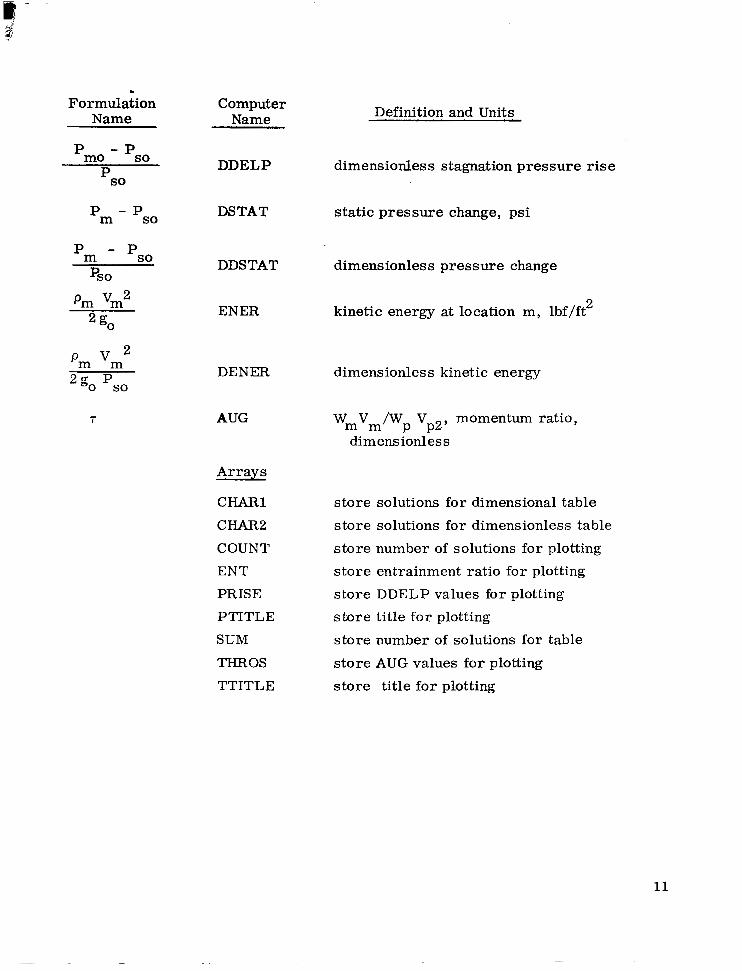
. Formulation

Name

'mo - 'so P so

'm - ' s o

'm - 'so pso

pm Vm2 go

2 Pm vm

2go pso

7

Computer Name

DDELP

DSTAT

DDSTAT

ENER

DENER

AUG

Arrays

CHAR1

CHAR2

COUNT ENT PRISE

PTITLE

SUM

THROS

TTITLE

Definition and Units

dimensionless stagnation pressure r ise

static pressure change, psi

dimensionless pressure change

kinetic energy at location m, lbflft 2

dimensionless kinetic energy

wmvm/wp Vp2, momentum ratio, dimensionless

store solutions for dimensional table

store solutions for dimensionless table

store number of solutions for plotting

store entrainment ratio for plotting store DDELP values for plotting store title for plotting

store number of solutions for table

s to re AUG values for plotting

store title for plotting

11

Section 3

ANA LYSIS

3 . 1 Formulation of the Mathematical Model

In this section an analytical model is developed to predict the flow be-

havior in a compressible flow jet pump with a constant-area mixing tube. The anal-

ysis is intended to provide a complete description of the important flow parameters

at specific locations within the jet pump and to describe the overall operation of the

jet pump as an entrainment and thrust augmentation device. The analysis was pre-

pared for air-to-air jet pumps. The parameters used i n the analysis are l isted i n

section 2. The geometr ical parameters are shown in figure 2.

The fundamental purpose of the analytical model is to develop the per-

formance characterist ics of the jet pump directly. These performance character-

istics can be represented by plots of jet pump pressure rise and momentum ratio as

functions of entrainment ratio for a number of values of primary jet pressures and

temperatures and for various area ratios. The performance characterist ics in this

form are analogous to head vs. capacity curves or performance maps which are

commonly used for pumps and compressors.

The equations describing jet pump performance and flow behavior include

the entrainment ratio as an independent parameter. The assumption of a particular

value for the entrainment ratio (together with the inlet flow p res su res and tempera-

tures and the primary-to-secondary flow area ratio) allows calculation of a l l of the

performance and flow parameters for that operating point, Then another value is

assumed for the entrainment ratio and the calculation procedure is repeated. Suc-

cessive points on the jet pump performance curves are determined in this way until

the complete curve is traced out. In the present calculations, the entrainment ratios

were l imited arbitrari ly to the range from 10 to 40. In some cases , the Mach num-

b e r of the flow in the accommodation region reached 1 . 0 for an entrainment ratio

less than 40. Higher entrainment ratios cannot be achieved in such cases because the constant-area mixing tube chokeswhen the secondaryflow Mach number reaches 1 . 0 .

12

3. 1. 1 " Assumptions - Used in the Analysis

The following assumptions are made to simplify the analysis without seriously compromising its accuracy:

1.

2.

3.

4 .

5.

6.

The values of specific heat at constant pressure (C)

and the specific heat ratio (k) a re exp res sed a s func-

tions of temperature; otherwise the gas is considered

to be a perfect gas.

Wall shear forces are assumed to be negligible when

compared to the pressure forces and the momentum of

the primary and secondary streams. (This assumption

is reviewed in section 3. 1.4.)

No heat is transferred across the wall of the jet pump.

The mixing tube is assumed to have a constant cross- sectional area along its entire length.

When the primary nozzle is operated at an off-design pres-

sure ratio, the primary jet is assumed to expand or contract isentropically until the primary and secondary streams have

equal static pressures. This adjustment process is assumed

to take place in the accommodation region between sections 1

and 2 (see figure 2 ) and is assumed to be completed before

any mixing takes place between the two s t r eams .

The stagnation temperature of the pr imary flow is assumed

to be sufficiently high that moisture condensation shocks do

not occur as the flow expands.

3. 1.2 Analysis of the Accommodation Region

The geometrical parameters and flow conditions in the jet pump are de-

fined as shown in figure 2 . The primary stream enters the accommodation region as a=

very high velocity jet; its Mach number may be as high a s 3 . 5. The large momentum of the

13

pr imary jet induces a secondary flow. In the region defined a s the accommodation

region, it is assumed that the primary and secondary jets do not mix, but the prim-

a r y jet expands or contracts unti l its static pressure matches that of the secondary

s t ream. At the point where the static pressures are equal, denoted a s section 2,

the accommodation process is assumed to be complete and the flows are parallel.

This accommodation process is generally accompanied by a series of oblique expan-

sion and contraction shock waves as the primary flow area adjusts to match the local

static pressure outside the jet. However, if the jet pump is operated close to itsde-

sign conditions, the degree of accommodation is small and the losses caused by the

shock waves will be small. A simplified oblique shock analysis indicates that a noz-

zle designed for 350 psia supply pressure can be operated down to 200 psis with

a total pressure loss due to shock waves of only 3%. For the values of supply pres-

su re to be considered here, the e r r o r introduced by treating both s t reams as i sen-

tropic flows is negligible. In fact, one of the aims of this research was to show thal

an assumption of isentropic flow during the accommodation process will produce

good results even when the system is operated at conditions quite far from the de-

s ign point.

A s long as the ratio of (P /Pso) is sufficiently high to guarantee a super- ! PO

sonic primary flow, as in the cases being considered here, the primary mass flow

rate may be calculated directly using equation (1). k + l ' k- 1 144x P (60 x At. C,S

w = P R 5 (1)

By specifying an entrainment ratio, m = Ws/Wp, the secondary stream

mass flow rate can a lso be found directly.

ws = m W P

In a perfect gas, the local values of total and static pressure a re re la ted

to the local Mach number by the following equation.

14

k k - 1

Po/P = (1 + - k - l M2) 2

At the end of the accommodation region, the static pressures of the primary and

secondary streams are equal. Therefore, at the end of the accommodation region

the following relation must be satisfied.

k k - k - 1 2 k - 1 k - 1 k - 1

P /(1+- ) P O 2 P2 2 Ms2 )

- Pso/ (1+ - - (4)

The mass flow rate per unit area for an isentropic flow i s given by the relation below:

The geometry of the constant area mixing tube requires that A p2 + As2 - Am* Using equation (5 ) to represent A and As2, and inserting the appropriate unit

conversion factors, the geometry condition becomes as follows:

-

P2

When W m, Ppo, P'

Pso, Tpo, Tso and Am a r e specified,equations ( 4 )

and ( 6 ) can be solved simultaneously to obtain M and Ms2. Equation (5 ) can be

used to find A and As2. P2

P2

Since the flow of both the primary and secondary streams is assumed to be isentropic in the accommodation region,values of s ta t ic pressure, temperature ,

and velocity can be obtained for each stream at location (2) by employing the follow-

ing equations.

15

k

k - 1 2

2 k - 1 p = P / (1+- P2 PO P2 )

T T / ( l + - k - 1 2 M ) P2 PO 2 P2

3.1.3 Analysis of the Mixing Region

The primary and secondary streams enter the mixing region with equal

static pressures and parallel velocities. In this region, complete mixing takesplace

and a uniform flow with constant properties across the channel is obtained at section

m. Treating the mixing region as a control volume with completely specified enter-

ing flows, the following equations can be applied.

Continuity Equation: Wm = W (1+ m) P (12)

Mass Flow Rate: Wm - - 6 0 X P m V A (13)

Equation of State: 'm - - p, R Tm/144 (14)

Momentum Equation:

16

Energy Equation:

where H is stagnation enthalpy;

V 2 H = P2

P2 cp2 Tp2 + 2 g o J

Hs2 - cs2 Ts2 + 2goJ 2

vs2 -

The equation for the specific heat at constant pressure for air as given in the "" Gas Turbine Engineering Handbook, G a s Turbine Publications, Inc. ,

1966, page 4, is presented below.

Ci = . 24916 - .482x Ti + .681 x (17)

Equations (13) and (14) are combined to give

Tm = 60 x 144 x (Pm Vm Am/R Wm)

Equation (15) is written in the form

and equations (16) and (18) are combined to yield

Since the values of T and Ts2 are known at the inlet to the mixing P2 region, Cp2 and C s 2 can be evaluated directly using equation (17). Equations (12),

17

(17), (18), (N), and (20) represent f ive equations for the f ive unknown exit parame-

t e r s , Wm, Tm, Cm, Pm and Vm. Therefore, these five equations represent a com-

plete set which describe the properties of the flow leaving the mixing section. In

most instances, T and Ts2 are sufficiently close in value to permit the use of a constant specific heat, Cp2 = Cs2 = C . This simplifies the solution by removing

equation (17) from the equation set.

P2 m

3.1.4 Jet Pump Performance Parameters

The jet pump performance parameters which are of particular interest

are the stagnation pressure rise and the momentum augmentation. These parame-

ters can be evaluated by using the following expressions.

A P t - P ( I + - - k-1 2 m 2 m ) - P s o

and 7 = outlet momentum/primary momentum

w v ( m + l ) V 7 = m m - - m

P P2 w v V

P2

During the jet pump test program, the measurement of the stagnation

pressure r ise produced by the jet pump proved to be difficult to accomplish. It was

much easier to measure the stagnation-to-static pressure r ise in the jet pump.

This pressure r ise can be used to define another jet pump performance parameter,

A Ps, which serves as an alternative to the stagnation pressure rise parameter, A Pt.

A P = P - P S m s o

All of the values needed to compute A Pt, A Ps, and T are provided by the

analyses of sections 3.1.2 and 3.1.3.

18

L

The analysis of the mixing region presented in section 3 . 1 . 3 neglected the effect of wall friction; this simplifies the equations describing the mixing process.

In this section, a procedure is developed to include the effects of wall friction in the jet pump analysis.

The mixing region was assumed to extend from the point where the pri-

mary and secondary s t ream pressures are equal to the point where they have merged

into a uniform flow with constant properties across the channel. In reality, the wall

friction effects occur in conjunction with the mixing process. Unfortunately, it is

difficult with the current state of knowledge to predict wall friction losses accurately

in the mixing region. Therefore, rather than adjust the mixing region analysis to

include the wall friction effects, we considered that it would be preferable at this time to treat the mixing process and wall friction as independent effects by imagining

the mixing tube to extend as shown in figure 3 beyond the point where the mixing

process is complete. The flow phenomena occurring in the mixing portion, segment

I , is a mixing process without wall friction as analyzed in section 3 . 1 . 3 . The fric-

tional portion, segment 11, represents the effect of wall shear forces upon a uniform

adiabatic flow. The hypothetical extension of the mixing tube is meant to represent the friction occurring within the actual mixing tube.

The effect of wal l shear forces in ducts is commonly represented by a

coefficient of friction defined as follows:

7 W f = 2

PV /28, where T is the shearing stress exerted upon the stream by the wall. The corres-

ponding stagnation pressure loss is given by equation (25). W

19

where

L = duct length

D = duct diameter

In many flow analyses, the value of the coefficient of friction is taken

from test results for pipe flow. The friction coefficient is a function of wall rough-

ness and Reynolds number. However, i n the case of the mixing tube, the wall fric-

tion occurs in a very non-uniform flow which has a high level of turbulence. The

value of the coefficient of friction for the mixing tube cannot be accurately determined

from pipe flow data. Therefore, it is convenient to represent the mixing tube wall

fr iction loss in terms of a head loss factor, KMT, which must be determined experi-

mentally. n L

- Pm vm

mixing tube - K~~ 2 go

The equations for an adiabatic flow in a constant-area tube with a stagna-

t ion pressure loss are given below. Primed variables denote parameters at the end

of the hypothetical extension of the mixing tube.

Momentum Equation:

k k 2

144 Pm(l + k-l 2 m M 2)m - 144 Pml(l + - k - 2 1 Mm .”)”= KNIT Pm 2go I’m (27)

Energy Equation:

V - m - - Cm Tm’ + -

2

C m T m + go go

Continuity Equation:

’m m ’m m v = ‘ V ‘

20

State Equation:

Definition of Mach Number:

These equations can be combined to give the following results: k -

'm M m t 2 (1 + 2 k - 1 M,'") = B

where

2 p = P k - 1

(3 5 )

(37 )

21

Eliminating P between equation (34 ) and equation ( 3 5 ) yields equation m (38) which can be used to determine Mmt .

After equation (38) is solved for Mmf, equation (34) can be used to determine P I .

Combining equations (29), (3O), (31), (32), and (33), an equation for Tml is obtained. m

Equation (33) is then used to determine Vm'

The equations developed in this section can be used to compute the values

of P m l , T m f , M m l , and Vm' fo r a jet pump when the "ideal" analysis of sections

3 . 1 . 2 and 3 . 1 . 3 is completed and the value of KMT is known or assumed. Alterna-

tively, these equations may be used to deduce the value of K when values of Pm',

Tm 3

puted by using the "ideal" analysis.

MT ' and Vm' are known from test resul ts and values of Pm, Tm, and Vm are com-

3 . 1 . 6 Dimensionless Formulation

In this section the equations describing the jet pump operation are for--

mulated in terms of dimensionless variables. The non-dimensional formulation is

valuable for two reasons:

According to the principles of dimensional analysis, a solution in terms of independent non-dimensional groups

is a general one. The same solution may be applied for

jet pumps having great differences in individual design or

operating parameters so long as the independent non-

dimensional groups are identical. For example, one

such group is the primary-to-secondary flow area ratio,

Ath Cu/Am; if all other non-dimensional groups are the

same , a large-scale and small-scale jet pump having

identical area ratios will have identical non-dimensional

performance characterist ics.

0 The non-dimensional formulation permits identification of

the minimum number of independent non-dimensional groups

22

4 -

which are required to completely specify a jet pump design

and its operating characteristics.

In the derivation which follows, unit conversion factors are not included,

and all values of the specific heats (C Cs, Cm) are assumed to be constant and equal.

P'

The equations which apply in the mixing region are given below.

Continuity Equation: W = W (1 + m ) m P (12)

Mass Flow Rate: - Wm - Pm 'm Am (4 0)

Equation of State : P = m Pm Tm (4 1)

Momentum Equation:

go Am (Ps2 - Pm) = Wm Vm - W V - m W V P P2 P s 2

Energy Equation:

T -I- m Tso = (m + 1) C PO

The dimensionless variables to be used are defined as follows.

v* = vm/vp2; P* = Pm/Pso, F = P /Pso, PO

- T = Tpo/Tso, A = Ath CJAm

-

Using these variables, equations (12 ), (40), (41), (42), and (43) can be combined a s follows,

P* (ps2/psO) + y [I + m (vS,/vp2) - (m + 1) v*]

(4 3)

(44 )

(45 1

23

k 2P*V* 6 m T v * ~ + - ( m + 1) ( l + = ) = 0

where

Y = wp ‘p2 o m so l g A and

(4 7)

The equations which govern the flow in the accommodation region are

developed next. F o r an isentropic pr imary s t ream,

and I 1

Equations (49), (50), and (5 1) can be combined to give

(52) so

24

Similarly, equati ons (44) and (51) can be used to obtain a value for 6 :

k - 1 1

Thus, y and 6 are shown to be functions of P, x, k and P /P s 2 so

The secondary stream velocity is given by equation (54):

Equations (49),

k - 1

(511, and (54)

Vs21Vp2 - -

can be combined to yield I k - 1 1

1 s - (52)-

k - 1 k

- [+ (E)] From the definition of total or stagnation pressure,

k - k - 1 2 k - 1

Ps2/Pso = 1 / (1 + - 2 Ms2 )

(54)

(55)

Considering equations (5 1), (53), (55), and (56) together, it can be seen

that the parameters y , 6 , Vs2/Vp2, and Ps2/Pso are functions of Ms2, P, T, A , m and k only. Equation ( 5 ) of section 3.1.2 can be written for the secondary s t r eam as follows.

25

Equation (57) can be combined with equation (50) and wri t ten in terms of dimensionless variables as given below.

k + 1

Ms2 k + 1

- -

F o r high entrainment ratio jet pumps, the term A /Am is of order 0.01.

Thus, the term (1 - A /A ) can be approximated as unity. Equation (58) can now be

written as follows.

P

P m k + 1

Ms2 2 2 ( k - 1 ) F K - -

k + 1 (+1) (5 9)

k- 1 2 2- (1'7 Ms2 1

Equation (59) shows that Ms2 can be determined from m, F, A, T, and k. This in-

dicates that y , 6, Vs2/V and P /Pso are functions of P, T , x, k and m. Re-

turning to equations (45 ) and (46), it can be seen that the performance of the jet pump

depends upon the parameters i?, T, x, k and m. For given values of P, T , E and k, a complete dimensionless solution can be obtained for each specified value of entrain-

ment ratio.

"

"

P2' s 2

"

The jet pump performance parameters can be experssed in the form of

dimensionless groups using the fundamental dimensionless parameters. The momen-

tum augmentation, T , is already a dimensionless group:

The dimensionless stagnation pressure rise parameter is defined as follows: k

26

k- 1 Apt * - - Apt = P* ( I+ 2 k- 1 2 -

Mm ) - 1

pso

!

To evaluate Apt *, it is necessary to know Mm2. Using the dimensionless

Mm2 is given by equation (62).

" 2

Thus, Apt * is a function of the fundamental dimensionless variables which

variables,

(62)

determine V*, P*, and . The s ta t ic p ressure r i se parameter , A P can be expressed

in dimensionless form as follows: S Y

APs* =

Equations (60) through (63) show that the dimensionless jet pump per-

formance parameters are functions of the fundamental independent dimensionless

variables F, T , x, k, and m. Five such independent variables and only five have

to be specified in order to determine the jet pump performance characteristics in

dimensionless terms. (This conclusion is restricted to jet pumps which satisfy the

assumptions listed in section 3.1.1 and the additional assumption that the specific

heats of all of the s t reams are equal , i. e . , C = Cp2 = Cs2 - - Cm . )

It is possible to use a different set of five independent dimensionless

variables. For example, a velocity ratio v = Vs2/Vp2 can be used in place of T to

complete an alternative set of five independent variables, F, V, A, k and m. An- other possible set is P, T , K , k, and v. The velocity ratio, 7, was one of the basic

design parameters used to select the jet pump geometry for the boundary layer COIF

trol system tested under contract No. NAS 2-2518.

"

These remarks can be summarized by the expressions below:

Jet Pump Performance Characterist ics

(dependent variables)

Design and Operating Conditions

(independent variables)

Apt *, APst and T are functions of F, T , K, k, m o r

27

3 . 1 . 7 Maximum Entrainment Ratio

Equation (59) can be used to determine the maximum possible entrain-

ment ratio. This maximum occurs when the secondary stream Mach number reaches

a value of unity. Setting Ms2 = 1 , equation (59) can be written as follows.

Thus, the maximum entrainment ratio corresponding to the choking of the secondary

stream can be determined directly from the dimensionless initial conditions.

3 . 2 The Computer Program

A computer program was prepared to predict the performance charac-

te r i s t ics of constant area jet pumps using the analytical concepts formulated in the

preceding sections. The program was written to develop both dimensional and di-

mensionless solutions. Values of P, T , x, Pso, Tso, and Am are read in as initial

conditions. Values of k, R , and m are included within the program. For each value

of m, values of T , Apt, APS, Apt*, and APs* are calculated. The values of 7 , Apt*,

and APs* depend only on t h e dimensionless data, while APt and APs depend also upon

”

pso, TsO, and Am.

The program is written in Fortran IV language. The machine used was an

IBM System 360/65 with an SC4020 plotter. Automatic plotting of the performance char-

acteristics was obtained by using the subroutine EZPLOT developed by the Missile Sys-

tems Division of Avco Corporation, Burlington, Massachusetts.

A block diagram of the computer program is shown in figure 4. For each

set of initial conditions, solutions are obtained for values of entrainment ratio between

10 .0 and 40.0 in steps of 3.0. The results a re printed as each solution corresponding

to a particular value of entrainment ratio is determined. The resul ts are a lso s tored

i n a r r a y s f o r plotting and for presentation in tabular form. A printout of the entire pro-

gram is presented in Appendix A. A discussion of the program by blocks is given in

Appendix B. Appendix C provides typical computer solutions which indicate the form of

the output data.

28

Certain of the blocks shown in figure 4 and described in Appendix B are

denoted as optional, indicating that they can be removed from the program without

interfering with the operation of the remaining blocks. Instructions for removing

these blocks are given in Appendix B, section B-2.

When frictional effects in the suction duct and mixing tube are to be taken

into account in the performance predictions, values of the loss coefficients K (defined in Appendix B) and QT must be provided as input data for the computer solu-

tion. These loss coefficients are functions of the flow Reynolds numbers. If values

of Ksd and KMT have been established for ducts of one size and the computer per-

formance predictions are to be used for ducts of much larger or smaller s izes , it may be advisable to adjust the values of the loss coefficients used by the computer

to account for t h e Reynolds number change.

sd

3. 3 Solutions . . ~~ ~~ for a Range - of Jet Pump Designs

The computer program was applied to develop jet pump performance

plots for a broad range of geometries and operating conditions. The range of solutions was selected to encompass all of the test conditions used in tRis investigation (sec-

tion 4) and also the range of conditions of interest to NASA for boundary layer con-

trol systems and momentum augmentation. The performance plots were developed for use in preliminary design of jet pump systems for matching the jet pump to a

duct system and for predicting the resulting system performance characteristics.

Techniques for applying the solutions to system design are described in section 3.4.

The range of conditions used to obtain the performance plots were ini-

tially defined in dimensional form as follows:

T pr imary flow stagnation temperature 450" F to 3500" F PO

P pr imary flow stagnation pressure 100 psia to 400 psia PO

Tso secondary flow stagnation temperature 20" F to 120" F

Pso secondary flow stagnation temperature 1500 psfa to 2116 psfa

The range of values selected for the corresponding dimensionless parameters were

a s follows:

29

T = 1 . 5 t o 8 . 0

= 5 t o 40

The nozzle and mixing tube geometries available for the test program had area

ratio values (A) ranging from 0.00125 to 0.0067. The range of values selected for

the performance plots is given below:

- A = 0 .001 to 0.007

The ranges of values of P, T, and 3 given above were used to prepare

9 s e t s of performance plots showing A Pt * vs. m and T vs. m for various values

of with T and fixed; these plots are indexed in table 1 and given in figures 6

through 23. Table 1 includes the values of maximum entrainment ratio attainable

for each combination of P , T , and x values. This maximum entrainment ratio is

s e t by choking of the secondary stream as given by equation (64) of section 3. 1.7 .

" -

Typical computer output sheets for one of the solutions are reproduced

in Appendix C. The printed output includes values of jet pump parameters not

shown i n the plots but required for the jet pump-duct matching techniques

described in section 3 .4 . These parameters are given in dimensional form based

upon standard secondary stream inlet conditions, = 2102 psfa, Tso = 7 0 ° F .

and A m = 0.08726 ft . 2 pso

In the l a s t six cases, the higher values of 6 cannot be attained because of

choking of the flow in the mixing tube. For the cases with T = 1.5 and 3.5, choking

occurs in the secondary flow (Ms2 = 1) as discussed in section 3.1.7. When T was

set at 8.0, choking was predicted to occur first at the mixing tube exit, i. e. , Mm= 1.

Cross-plots showing AP * vs. m and T vs. m for various values of A with and fixed are presented in figures 24 and 25. Lines of constant mixing

exit Mach number a r e a l s o shown. These cross-plots provide additional insight

the effect of the area ra t io upon jet pump performance.

t tube

on

30

3.4 Jet Pump-Duct Matching Considerations

The previous sections have developed analytical techniques and a cam-

puter program which allow prediction of the performance characteristics of high-

entrainment-ratio jet pumps. The performance characteristics take the form of

plots of jet pump pressure r ise and momentum ratio as functions of entrainment ra t io for a number of values of primary jet pressures and temperatures and forvnr-

ious area ratios. These performance characterist ics are analogous to head v s . ca-

pacity curves or performance maps which a r e commonly used for pumps and com-

pressors. The actual point (i. e. , entrainment ratio) at which a jet pump will oper-

ate when connected to a particular system of inlet and discharge ducts is dictated by

the geometry of the duct system.

The resistance curve of a duct system is roughly parabolic as shown in

figure 26. A typical jet pump characteristic is also shown on the figure . The actu-

al operating point of the jet pump-duct combination is defined by the intersection of the two curves. The duct characteristic curve is se t by the duct geometry and is

essentially independent of the jet pump operating conditions. Therefore, i f the duct

geometry is not changed, the operating point of the system for any jet pump primary flow condition must be located on the parabola. Figure 27 shows how the operating

points for a system can be determined if the jet pump performance at various pres-

sure levels is known.

This section establishes a procedure for use to determine the operating

points of a jet pump in a duct system when the loss characterist ics of the duct sys-

t e m a r e known. This procedure can be employed a s shown by example to match the

jet pump design to the duct system so a s to achieve maximum entrainment ratio or maximum thrust augmentation for given primary flow conditions.

3.4. 1 R-egnttion .~ of Duct Loss Characterist ics

When the analytical model developed in sections 3 . 1 and 3 . 2 is suppliedwith values of P , T and A , the performance parameters such as stagnation pressure r ise and momentum ratio (thrust augmentation) can be calculated a s a function of entrain-

ment ratio. In order to determine the specific value of entrainment ratio which will

”

31

be obtained during operation of a given jet pump of fixed geometry, the associated

duct system flow character is t ics must be taken into account. Using the notation

shown in figure 2 , the stagnation pressure rise may be written as follows:

The two bracketed terms together represent the stagnation pressure loss of the duct

system including the inlet duct (first term) and blowing duct (second term).

At low Mach numbers, the stagnation pressure loss due to friction i n a duct is proportional to the kinetic energy of the flow. For high entrainment ratio

jet pumps, the mass flow rates in the suction and blowing ducts are nearly equal.

Therefore, the total pressure loss of the entire ducting system may be related a s a

first approximation to the kinetic energy of the blowing duct inlet flow by equation (66):

('mo - pb0> + (pa0- ps0) = K Q 'm"m go

This type of expression has been shown to be accurate for representing frictional

losses in duct systems of various shapes.

3 . 4 . 2 Evaluation of the Loss Coefficient, I(

The loss coefficient K depends on the geometry of the particular ducts B being used and the Mach number level (ref.13). At sufficiently low Mack numbers,

(i. e. , under 0.3), compressibility effects can be neglected. For flows a t higher Mach

numbers, the value of KQ can be corrected for compressibility effects.

Loss coefficients have been presented for a number of duct configurn-

tions in references 13 through 26 I The configurations reported include ducts of rec-

tangular and circular cross section with varying amounts of diffusion o r acceleration.

Bends and elbows having a number of different angles of turn are included in these

references. The loss coefficients reported were measured for subsonic flow cover-

ing a range of Mach numbers up to 1 . 0 .

32

To provide an example of typical loss data, the influence of Mach num-

ber level upon the loss coefficient for straight, conical diffusers is shown in figure

28. The variation of K with inlet Mach number is significant for a diffuser of specified geometry.

Q

Because the value of K is closely related to the duct configuration and Q the Mach number level, and values of K are readily available for only a few simple

duct shapes, the designer of a jet pump and duct system generally will not be able to

look up an accurate value for K for a new duct design. If optimum matching of the

jet pump and ducting is required, the loss coefficient of a new duct geometry will

have to be determined experimentally. Testing can be done by using either a ful l -

scale o r reduced scale model of the duct. The tests must cover the Mach number range which will be encountered by the actual duct when operating with the jet pump.

Flow tes t s of ducts sometimes have additional value; regions of flow separation or

undesirable velocity profiles may be revealed. When the duct geometry is modified

to eliminate these problems, the loss coefficient is usually reduced.

Q

11

3.4. 3 Development of System Performance Equations

At the outlet of the blowing duct, the static pressure in the flow must be

equal to the local "atmospheric" pressure. The use of a blowing duct having the

same cross-sect ional area a s the constant-area mixing tube will limit the entrainment ratio which can be achieved in the jet pump system. Higher entrainment ratios

can be obtained with the same jet pump if a diffuser is added to theblowing duct. The

diffuser allows higher velocities and flow ra t e s in the mixing tube. The mixing tube

pressures can be sub-atmospheric; the diffuser decelerates the flow to increase its

s ta t ic p ressure up to the atmospheric pressure level at the blowing duct exit.

A calculation method can be developed for use to determine the actual

operating point (i. e. , entrainment ratio) for a jet pump system as a function of the

area ratio selected for the blowing duct diffuser. The calculation method makes use

of the generalized jet pump performance characteristics developed by the computer program described in section 3. 2 and Appendix B.

33

The loss coefficient defined in equation (66)is inserted in equation (65)

with the following result:

where 9

'm m v " go

- - 'm

Equation (67)may be rewritten a s follows:

l P t = (Pb-P ao ) + K q + (Pbo-Pb) B m (68)

The term (P -P ) represents the external ambient pressure difference imposed

upon the jet pump system. This term will be called A Pext: b ao

The value of 4 Pext was zero for the experimental jet pump since both

the discharge static pressure (P,) and inlet stagnation pressure (Pao) fo r the jet

pump system were equal to atmospheric pressure. This term is not necessarily

zero for jet pump systems which operate in the presence of an external velocity

field. For example, a jet pump used for boundary layer control at the trailing edge

of a wing will have its inlet pressure (Pao) established by the flow behavior in the

suction slot entry passages and by the local pressure acting on the wing. The dis-

charge pressure (P,) will be set by the local pressure field on the wing and by the

flow behavior from the slot to the deflected flap.

The term (Pbo - Pb) in equation(G8) represents the dynamic head of the

flow at the blowing duct exit. This term is related to the blowing duct exit Mach

number a s shown in equation(70) : 1,

34

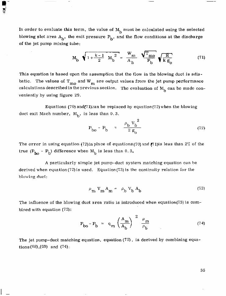
In order to evaluate this term, the value of M must be calculated using the selected

blowing slot area Ab, the exit pressure Pb, and the flow conditions at the discharge

of the jet pump mixing tube:

b

This equation is based upon the assumption that the flow in the blowing duct is adia-

batic. The values of Tmo and Wm a r e output values from the jet pump performance calculations described in the previous section. The evaluation of M can be made con-

veniently by using figure 29. b

Equations (70) and(7l)zan be replaced by equation(72) when the blowing duct exit Mach number, Mb, is less than 0 .3 .

The e r ro r in using equation (72)in place of equations(70) and P1)is l e s s than 2% of the true (P - P ) difference when Mb i s l e s s than 0.3. b o b

A particularly simple jet pump-duct system matching equation can be

derived when equation(72)is used. Equation(73)is the continuity relation for the blowing duct:

p, V m A m = p V A .b b b (73)

The influence of the blowing duct area ratio is introduced when equation(73) is com-

bined with equation (72): n

The jet pump-duct matching equation, equation (75), is derived by combining equations(68),(W and (74):

3 5

I -

2

A p t = 4 P

f o r

Mb 5 0 . 3

For preliminary design purposes, the value of pm/pb can be taken a s 1. 0. A more accurate value can be determined as follows:

For a perfect gas,

With Mb less than 0 .3 , equation(77) holds with an error of less than 2%:

Tb Tbo (7 7 )

Since the flow in the blowing duct is adiabatic, its stagnation temperature remains

constant; = T 173s mo

The last relation required is equation (79):

k - 1 2 ” Tmo - I + - Tm 2 Mm

When equations (76) through (79) are combined, an equation for calculating pm/p

is derived: b

36

Equations (74), (752, and ( 8 0 ) san be used with small error only if M b i s less than 0 . 3 . If M i s g r e a t e r than 0 . 3 , the jet pump-duct matching equation,

equation (81), is der ived by combining equations (68), (G9), and (70): b

for all values of Mb

where Mb is computed by using equation(71) and figure 29.

The re a r e two figures of merit which are of interest in the evaluation of

jet pump systems for boundary layer control or thrust augmentation applications.

These figures of merit are the entrainment ratio and the thrust augmentation. The

equations developed above can be used to determine the entrainment ratio at which a jet pump system will operate. Several additional equations are required in o rde r

to calculate the thrust augmentation obtained from a jet pump system.

The thrust augmentation obtained with the complete system is defined in equation (82):

X = system thrust augmentation

wm 'b w v

P P2 T T =

The thrust augmentation produced by the jet pump alone was designated a s T i n section 3. 1 . 4 (equation 22) . The computerized jet pump performance analysis of section 3 . 2

provides as output data values of T a s a function of entrainmentratio. Thus, once

the entrainment ratio is known for a j e t pump system, the value of T i s known and

the system thrust augmentation can be calculated as follows:

wm Vm 7 = w v

P P2

so

The value of Vb/V, can be related to the blowing duct area ratio by using equation

(73) :

" vb 'm m 'm 'b A b

A "-

The value of pm/pb is given by equation (80) when Mb 5 0 . 3 . When % exceeds

0.3, the value of pm/pb is given by equation (8 5) :

(1+ - k - 1 2 "- 'm - 'm Mm ) 2

'b

where the blowing duct flow has been assumed to be adiabatic and the value of Mbis

determined by using equation(71) and figure 29.

The equations given above can be used to compute the thrust augmen-

tation parameter once the operating point of the jet pump is known. The next section establishes a procedure for determining the operating point.

3.4.4 Calculation Procedure fo r Determining the Operating Point of a Je t Pumr, in a Duct Svstem

The operating point of a given jet pump and duct combination can be de-

termined as follows:

Required Initial Data :

Given: Jet pump design and performance characteristics:

basic jet pump parameters

38

jet pump performance curves; output data from computer program

values characterizing the particular duct system

Solution technique if Mb 5 0. 3:

The specified values of KQ , A Pext,

A P t vs m

qm v s m

Mm vs m Pm v s m

KQ * 'ext 'b *b

P , and A are inserted into equa- b b tions (80) and (75 ) . The jet pump performance curves are used to find associated

values of L\ Pt, Mm, and Pm which satisfy equation ('75). This is a trial-and-

error process which is begun by assuming a value for entrainment ratio, m. The corresponding values of Mm and Pm are determined from the jet pump performance

curves and entered into equation (80). The resulting value of pm/pb is entered,

together with the value of qm from the jet pump curves, into the right-hand side of equation (75). If the resulting value of A Pt does not agree with the curve value, a

new value of m is assumed and the process is repeated. The iteration process is

simplified by graphical solution techniques which are described in the section entitled "Sample Calculation". This calculation process finds the value of m a t which the jet pump system will operate with the selected value of A

'm 9

b'

Solution technique if M > 0.3: b

The specified values of KQ , A Pext, Pb, and A are inserted into equa-

tions (81) and (71), The jet pump discharge flow ra t e , W and the stagnation tem-

perature of the discharge flow, Tmo, are plotted a s functions of entrainment ratio,

m. Values of Mb c m be determined as a function of m using equation (7l)and figure 29. The solution technique is a trial-and-error process which is begun by assuming

a value for m. The jet pump performance curves are used to f ind values of qmand

b

m'

39

I -

--- I

A Pt for each value of m assumed. Corresponding values of M are de te rmined as

above and entered with the qm values into the right-hand-side of equation (81). If

the resulting value of A Pt does not agree with the curve value, a new value of m is assumed and the process is repeated. Graphical solution techniques, described in the section below, can reduce the number of iterations required.

b

Evaluation of thrust augmentation:

The solution techniques described above yield the value of entrainment ratio at which a jet pump will operate in a selected duct system. The performance

data provided by the jet pump computer program allows determination of the values

of the following jet pump performance parameters at the operating point: T , pm,

Mm 9 Wm, and Tmo. by using the equations presented at the end of section 3.4.3.

These values allow calculation of the thrust augmentation, TI,

Additional Comments:

The values of K P and Pso a r e not constant for all values of entrainment

ratio. At high entrainment ratios, the Mach number levels within the ducts may

become sufficiently high that the influence of compressibility upon K must be taken

into account. Similarly, the value of P which is a non-dimensionalizing param-

eter in the jet pump performance analysis, varies slightly as shown in equation (86)

when the entrainment ratio (and secondary stream flow rate) changes.

Q so’

pso - - where gm varies with m

The variations of K and Pso with entrainment ratio are generally second-order in

magnitude. These variations can be neglected in preliminary design calculations,

then included for final design if K and K. a r e known a s functions of the Mach num-

b e r Mm S Mi.

P

P 1

3 . 4 . 5 Sample Calculation

The use of the procedure described above to determine the operating

point of a jet pump-duct system is illustrated by the sample calculation which follows:

40

The jet pump design data is:

P = 300 psia PO -

P = 20.13

pso = 14.9 psia

T = 1200" F

- 80" F PO 1 -

T = 3.074 -

Tso

Am

AthCw'

= 0.08726 ft2 1 - A = 545.4 (Test value for the Case 4

0.000165 ft2 nozzle)

me computer solution for the jet pump performance yielded the values given in

table 2 . The values of A p t , p,, Mm, and qm a r e plotted against entrainment

ratio in figure 30.

The duct system design conditions were assumed to be as follows:

A Fext = 0 (i.e. , Pb = P ) ao

KQ

'a o

= 0 . 1

= 14.9 psia

The blowing slot discharge Mach number, Mb, was assumed to be less t h a n 0 . 3 .

Using these values in equation ('75) equation (87) was derived.

The calculations were begun for a blowing duct diffuser area ratio,

(A /A ) , equal to I. 0. Three values of entrainment ratio, m = 13, 15, and 1 7 ,

were selected arbitrari ly. The corresponding values of A Pt, Mm, qm, and Pm

were read off from figure 30. These values were used to compute pm/pb from

b m

4 1

equation (80) and then to compute the right-hand side of equation(87) ; the right-

hand side will be called A Pt ) trial. The results are given in the table below.

F o r Ab = 1.0 :

m ) A Pt qm pm - 'm * Pt tr ial (PSf) Mm ( p s ~ psia 'b @sf)

13 99.6 .205 65.3 15. 15 1.02 74.9

15 98.5 .235 87 15.00 1.01 96.8 17 97.5 .270 109 14.80 1.01 12 1

The A Pt) trial values can be plotted against entrainment ratio as shown in figure 31 . The intersection of the A Pt) trial curve with the A P jet pump performance curve

represents the solution of equation (87) for the selected value of Ab/Am. This in-

tersection is the operating point of the jet pump in the specified duct system.

t

3.4.6 Influence of Blowing Duct Area Ratio and Duct Losses Upon Entrainment

Similar calculations were carried out for values of Ab/Am equal to 2, 3 ,

and 4. The resu l t s a re shown in figure 31. The entrainment ratio increases as the

blowing duct area ratio is increased; the trend is more ulearly shownwhen the results

are replotted as in f igure 32. For the particular jet pump and system design condi-

tions assumed for this sample calculation, the maximum entrainment ratio is

achieved when the mixing tube is choked, i . e . , when Ms2 = 1.0.

The influence of the duct loss coefficient was explored by setting K t =

0.2 instead of 0.1 as previously assumed. The duct matching calculations were repeated using equation (75); the resu l t s a re shown in figure 32. Only a small increase

in entrainment ratio can be obtained by increasing the area ratio from 4 to 5. This

is a consequence of the fact that, by using a sufficiently large area ratio in the blow-

ing duct diffuser, the term (Pbo - Pb) in equation(G8)can be reduced to almost zero.

In that case, equation (75) takes the following form:

42

A p t = A P + Km qm ext

for small values of A,/A~

The maximum value of entrainment ra t io is the value for which equation (89) holds:

A 't - A 'ext

In the present example, with K = 0.2 and A Pext = 0, the limiting value of entrain-

ment ratio is found by use of figure 30 to be 34. The corresponding mixing tube exit

Mach number, Mm, is 0.615.

I

The resu l t s show that the maximum entrainment ratio which can be

achieved in a duct system driven by a particular constant-area jet pump is s e t by one of two conditions:

o r

0 by choking at the mixing tube outlet o r the suction duct inlet (i. e. , Mm= 1. 0 or M = 1. 0) if the duct losses are

sufficiently low s2

0 by the duct loss limit which is represented by equation

(89) if the value of Mm remains below 1.0.

The form of equation (75) is such that, along curves representing con-

stant values of Kt , an increase in blowing duct diffusion always yields an increase

in entrainment ratio until the limiting value is reached. In practice, K is a variable which depends upon the diffuser area ratio. In jet pump systems with low-loss inlets, the value of K is determined primarily by the blowing duct loss coefficient

which increases as the area ra t io increases . This t rend is shown for conical diffusers in f igure28. Examples of the effect of the variation of Km a r e shown by the

dashed curves in figure 32; these curves represent the loss character is t ics of 15" and 20" conical diffusers. The peak entrainment ratio for the 20" diffuser is achieved by using an area ratio of 3.; higher area ratios lead to reduced entrainment because of increased losses.

e

e

43

3 . 4 . 7 Influence of Blowing Duct Area Ratio and Duct Losses Upon Thrust Augmentation

Figure 33 shows the thrust augmentation parameter, I-, for the jet pump

itself. This curve is taken directly from the computer calculations for the jet pump

selected in section 3.3.5. In o rde r to determine the values of the system thrust

augmentation parameter PIT in relation to the blowing duct diffuser area ratio A d A m and the loss coefficient M figure 32 was used to determine the entrainment ratio

corresponding to selected values of Ab/Am and KQ . Then f igu re 33 was used to find

the associated values of T. The equations of section 3 . 4 . 3 permitted calculation of

T .

P '

The variation of system thrust augmentation with blowing duct diffuser

a rea ra t io is shown in figure 34. The curve for K = 0 yields maximum thrust aug-

mentation when the mixing tube is choked, i. e, for Mm = 1.0. Even with a very low

loss in the duct system (Kt = 0. 1)9 the thrust augmentation reaches a maximum

value at a mixing tube Mach number less than 1.0. The curves for K = 0 . 1 and

0.2 show that the thrust augmentation does not fall off rapidly if the diffuser area

ratio is made larger than optimum. This suggests that , when designing a duct sys-

tem without complete data on duct losses, it is preferable to err on the side of in-

creased diffusion.

Q

P

The relationship of system thrust augmentation to the entrainment ratio

i s shown in figure 35. The thrust augmentation peaks on the curve for K = 0. 1 and

0 . 2 and then falls off with increasing entrainment ratio. This is a consequence of

the fact that the thrust augmentation is proportional to the product of entrainment

ratio and blowing duct exit velocity a s follows:

P

where (m + 1) fi: m for high entrainment ratio jet pumps and V constant

P2

so TI-= 'b

44

In order to achieve entrainment ratios higher than the value at the peak of the TT curve, the diffuser area ratio must be increased. This has the effect of reducing

the exit velocity Vb faster than entrainment increases. The net effect is a reduction

of the product m Vb and thus TT.

The maximum entrainment ratic. attainable is set by the choking limit

for the Kt = 0 and Kt = 0 . 1 cases . For the Kt = 0 . 2 case, the maximum entrain-

ment value is se t by the duct loss limit as represented by equation (84). At this

l imit , the diffuser area ratio is very large and the duct exit velocity is zero. Con- sequently,lTmust be zero a s shown by equation (85). This illustrates the general

rule that the thrust augmentation in a jet pump system is always zero at maximum

entrainment unless the jet pump mixing tube is choked.

3.4. 8 Conclusions

The two previous sections have shown the influence of duct losses and

blowing duct diffuser area ratio upon the entrainment ratio and thrust augmentation

obtained in a jet pump-duct system. The results shown in figures 32, 34, and 35 a r e

quantitatively valid only for the particular jet pump geometry and operating conditions

which were chosen i n the section 3 . 4 . 5 . However, the figures illustrate trends which a r e qualitatively correct for high entrainlnent compressible flow jet pumps as a gen-

e ra l class.

The results show that the design goals of maximum entrainment and maxi-

mum thrust augmentation may require different duct geometries; a system designed

for maximum entrainment may have a low value of the thrust augmentation parameter

and vice versa. The influence of duct losses is shown to be very strong. Entrain- ment ratios and thrust augmentation both can be improved significantly by making

only minor reductions in the duct loss coefficient. This provides considerable in-

centive for testing flow models of proposed new duct designs in order to adjust their

geometry to achieve minimum losses. Accurate estimates of duct loss coefficients

can be obtained from these tests; such estimates are required in order to predict the

performance of a new jet pump system and to allow selection of the best diffuser area

ratio.

45

The design problem for a jet pump system often takes the following form:

Given: Pr imary flow pressure, temperature, and flow rate

Duct system inlet and discharge pressure levels and

inlet pressure

Problem: What is the proper mixing tube area and blowing

duct diffuser area ratio to be used to achieve the

design goal, e. g. , maximum entrainment o r thrust

augmentation ?

The information provided in plots like figures 32, 34 , and 3 5 , together with duct loss

estimates, will allow the designer to evaluate the effect of diffuser area ratio upon

entrainment ratio and thrust augmentation for a selected mixing tube area. By pre-

paring similar sets of curves for several other values of mixing tube area, the de-

signer can chose the best combination of mixing tube area and diffuser area ratio to

meet the design goals. New jet pump performance curves analogous to figures 30and

32 will be required for each value of mixing tube area to be considered. Data for

these performance curves can be obtained by using the computer program described

in section 3 . 2 A series of computer solutions covering a broad range of j e t pump

geometries and operating conditions is provided in section 3. ? for use in preliminary

design calculations.

46

Section 4

TEST PROGRAM

The test program had two major objectives:

0 to provide data for use to evaluate the analytical model

0 to determine whether new, reduced-blockage nozzle

clusters could be used to improve the performance of the original jet pump

Pr imary Flow

pressure range 55 psia to 400 psia temperature range 200" F to 1200" F

nozzle throat area range 1 . 1 x ft2 to 6 .0 x ft2

nozzle cluster three designs

nozzle geometry four designs

Secondary Flow

inlet pressure laboratory ambient inlet temperature laboratory ambient

mixing tube geometry constant area = .087 ft2, two lengths

p re s su re rise regulated by discharge throttling device

This section of the report describes the jet pump test arrangement, the test program,

and the results which were obtained.

4.1 Test Arrangement

The jet pump test arrangement with its instrumentation is shown schemat-

ically in figure 36. The pr imary flow supply system employed a 2-stage reciprocating

47

compressor capable of supplying 7 lbm/min of a i r a t 400 psia. Electrical heaters

were used to achieve temperatures up to 1200" F. The primary flow was delivered

to a multiple-nozzle cluster directed along the axis of a constant-area circular mix-

ing tube.

The momentum of the primary flow entrains a secondary a i r flow from

the room into the bellmouth inlet and then into the mixing tube. Here, the two s t r eams

mix together and the stagnation pressure of the secondary stream is increased. The

flow from the mixing tube passes through a conical diffuser and exhausts to the atmos-

phere through an adjustable throttling cone.

The individual components of the experimental jet pump are descr ibed

below:

1. Calibrated bellmouth inlet section.

This component consists of a wooden bellmouth, metal

connecting tube, and fiberglass primary flow inlet section.

The bellmouth differential pressure was calibrated in t e rms

of flow ra t e by using an orifice and blower available in the

laboratory. The calibrated bellmouth permitted direct meas-

urement of secondary mass flow ra te for a l l j e t pump tests.

A ceramic insert was used to protect the f iberglass duct

from the hot primary flow pipe and flange.

2. Mixing Tube

48

The original variable-area mixing tube from the previous

investigation (ref. 12) was used for the f i rs t tes ts in order

to provide baseline performance data. This mixing tube had

a length of 6.87" (figure 37). After the initial tests were completed , the

mixing tube was bored out to a constant inner diameter of 4.000".

A mixing tube extension of the same diameter was also fabri-

cated. The remainder of the test program was completed using

both the original mixing tube length of 6 . 87" and the extended

mixing tube length of 18.87".

3. Conical Diffuser

The initial section of the conical diffuser had a length of

10.98" and an area ratio of 1.79. This diffuser section was

previously used during the Wagner BLC system tes ts . An additional section was added to this diffuser to obtain an over-

a l l area ra t io of 5.0. The purpose' of the exhaust diffuser was

to maximize the static pressure recovery so that the highest possible system entrainment ratio could be achieved. Changes

in the axial positioning of the throttle cone in the diffuser dis-

charge produced a variable system resistance. The jet pump

performance characterist ic (pressure r ise versus entrainment

ratio) was generated by varying the system resis tance in this

manner,

4. Nozzle Cluster Geometry

The nozzle cluster geometry used in the previous investiga-

tion (ref. 12) was believed to cause excessive blockage of the

secondary flow at the mixing tube inlet, thus causing reduced

performance. of the jet pump system. Two "reduced-blockage"

nozzle cluster configurations were tested in order to determine

whether improved performance could be achieved.

The first reduced blockage nozzle cluster was made by placing

2.0" long nozzle extensions between the original nozzle cluster

body and each of the nine nozzles. This change moved the clus-

ter body back away from the mixing tube inlet in order to reduce the velocity level around the cluster by increasing the adjacent

flow a rea . This change is shown on figure 38,

The second reduced blockage nozzle cluster was a completely new design consisting of 7 nozzles at the end of small diameter

tubes (1/4" dia. ). This low drag c luster is shown on figure 39.

49

5. Primary Nozzle Geometry

Five sets of pr imary flow nozzles were used in the test program.

The throat size, nozzle type, and design conditions are listed in

table 3.

The first four nozzle sets listed in table 3 were used with the original

nozzle cluster and also the first reduced-blockage configuration (original cluster

with 2" extension tubes). The fifth set, Case LD#2-4, consisted of seven nozzles

for the second reduced-blockage cluster. The Case LD#2-4 nozzles were designed

for the same operating conditions a s the Case 4 nozzles of the original cluster.

The nozzle flow coefficients listed in the table were calculated from test results according to the definition below:

W

cW =P

ideal W

where

W = measured nozzle flow rate a t design pressure and P

temperature

W = isentropic flow rate through nozzle throat at design

pressure and temperature; based upon one-dimensional

flow assumption

4.2 Instrumentation and Data Reduction P r o c ~ ~ d u r e s

4.2.1 Instrumentation

The instrumentation used to determine the performance of the experi-

mental jet pump is shown on figure 40 and described in table 4.

The jet pump inlet bellmouth was calibrated for use as a f lowmeter. The

calibration was accomplished by connecting the bellmouth and the suction duct to the

inlet of a blower. An orifice and a throttling arrangement were included in the blower

system. The blower permitted calibration of the bellmouth up to a flow rate of 200

l b d m i n . The resulting bellmouth flow equation is given on the following page:

50

wS

where

A hb = P differentia1 pressure, inches of water gage b

= inlet density, lbm/ft 3 pb

Stagnation pressure traverses were made in the mixing tube and diffuser with a Kiel probe. When the short mixing tube configuration was used, traverses

were taken only in the diffuser a t the location shown in figure 4 0 . When the mixing

tube extension was used, stagnation pressure traverses were taken in the tube 16.4 inches downstream from the primary nozzle exit plane. Additional traverses were

made in the diffuser 26 .4 inches downstream from the primary nozzle exit plane.

The angular orientation of the traverse locations is shown on figure40 . The same numbering system was used for all traverse locations.

4 . 2 . 2 Data Reduction Procedures

The measured data were used to calculate the following jet pump per-

formance parameters .

wS m = - W - jet pump entrainment ratio

P

'm - 'so A P s = - jet pump static pressure

pso parameter

* A P A =

pmo - pso n - jet pump stagnation pressure

L r s o rise parameter

2 v vs. (F) r - velocity profiles

0

P vs. distance

P vs. m and P - jet pump static pressures

PO

51

The static pressure parameter was calculated using the wall static pres-

sure measured at the discharge of the short mixing tube or the maximum static pres-

sure reached within the extended mixing tube. The secondary flow stagnation pres-

sure a t the mixing tube inlet (P ) was determined by subtracting the measured bell-

mouth inlet and cluster loss (section 4.2.3) from the barometric pressure. so

The jet pump stagnation pressure rise parameter, A Pt , is based upon

the secondary flow total pressure Pso and upon P Our f irst tests showed that it

was not possible to measure Pmo accurately with the "short" mixing tube, i. e. , the original 6 . 87" mixing tube length. Complete mixing was not achieved by the end of

this short tube; sharp velocity peaks corresponding to the primary flow jets were ob-

served at the exit section. These peaks were too sharp to be accurately measured by stagnation pressure probes of reGsonable size. Therefore, the stagnation probe measurements could not be used to determine P with the necessary accuracy.

*

mo'

mo To obtain an approximate value of Pmo for the short mixing tube tests we

used the following procedure:

Stagnation pressure probe traverse data was taken a t the conical diffuser exit section, Pdo in figure 40. This data was used to de-

termine an average stagnation pressure (P ) by procedures described below. Then the value of Pmo was computed by using equation (92) which accounts for the diffuser stagnation pressure loss.

do

n 17 2

52

The value of K was selected to be 0 .05 , a value representative of

the loss coefficient for a good diffuser.

The procedure used to determine an average stagnation pressure

from the stagnation pressure probe readings was the "mass-momentum

integral method". The stagnation pressure was measured along a diameter

a t the diffuser traverse location. A wall static pressure measurement

was obtained a t that cross-section. Using the ratio of the local stagnation

pressure and the wall static pressure at each point along the diameter,

the local Mach number was determined. Using a plot of (1 + kM ) vs.

cross-section area (i. e. , r /r ), the impulse function was determined

by graphical integration:

2

2 2 0

cp = impulse function = P I (1 + kM2) dA (-93)

The following equations were used to determine the "mass momentum"

averaged properties of this non-uniform compressible flow:

- calculate P (static) from: P = -

(1 + kG2) A

k - k- 1

- calculate P (stagnation) P = F [ 1 +(?I -

from: 0 0

These "mass-momentum average" values of pressure satisfy the

measured mass flow r a t e and integrated momentum of the flow.

They correspond to values that would be obtained if the actual non-

uniform flow was mixed to a uniform flow in a frictionless, constant area duct.

To calculate Pm0 for the extended mixing t.ube, the "mass momentum

integral method'' was applied to the traverse data taken in the mixing tube 16 .4"

downstream from the primary nozzle exit plane. No correction for diffuser losses was needed in this case.

The velocity profiles were calculated from the local values of Mach num-

be r and the measured jet pump exhaust temperature (T ). eo

4 . 2 . 3 Suction Duct and Nozzle Cluster Losses

In order to calculate the jet pump pressure r ise parameters .IPS and * A Pt , the mixing tube inlet stagnation pressure P is required. The value of Pso

was determined by subtracting the appropriate suction duct and nozzle cluster so

53

stagnat ion pressure losses f rom barometr ic pressure (the suction duct inlet stagna-

t ion pressure). The loss data used for the determination of Pso is given below.

Bellmouth Inlet

The stagnation pressure losses in the bellmouth, suction duct, and nozzle

cluster configuration used in the test rig (figure 36) were measured for the following

four configurations:

1. Original nozzle cluster

2. Original nozzle cluster'with 2Ic nozzle extensions (figure 38)

3. "Low-dragll nozzle cluster (figure 39)

4. No nozzle cluster

The loss measurements were made by connecting the jet pump including the initial

section of the conical diffuser (area ratio 1.79) to the suction line of a blower and

orifice installation. Air was drawn through the bellmouth and jet pump system by

the blower. The stagnation pressure at the end of the constant area mixing tube was

calculated using the measured wall static pressure and the Mach number(computed

on a one-dimensional basis) at the same measuring station. The stagnation pressure

loss was set equal to the difference between this value and the atmospheric pressure.

The loss values for the four nozzle configurations are presented on figure 41. These

loss values include the suction duct loss, the nozzle cluster loss, and the short mix-

ing tube wall friction loss (L/dm = 1.35) .

The results show that the losses are identical for the two reduced block-

age clusters #2 and 3. A comparison of the losses for the low blockage clusters to

the losses for the original cluster and the minimum possible losses (the "no cluster"

curve) shows that the reduced blockage clusters cut the cluster losses by about427;.

These results were used for two purposes:

1. to guide the selection of the 'foptimum" nozzle cluster

54

2. to permit calculation of P at the jet pump inlet by sub- so

tracting the suction tube and nozzle cluster losses from

the atmospheric pressure. The Pso value was used to

calculate the static pressure parameter 1 Ps * and the

stagnation pressure rise parameter A Pt*.

BLC Suction Duct

The data obtained during tests of the Wagner BLC system under the previous contract NAS 2-2518 indicated that the aerodynamic drag of the present nozzle

cluster was much higher than had been expected. This drag was considered to be

one of the principal reasons for the difference between the predicted and actual performance of the jet pump BLC system. To check this point, the NAS 2-2518 suction

duct (figure 4 9 , the short mixing tube, and the initial section of the conical diffuser

were connected to the inlet of the blower and orifice system. The original nozzle

cluster geometry was installed in the suction duct. The tests results are shown on

figure 41. The BLC suction duct produced higher losses than the bellmouth config-

urations.

Still using the NAS 2-2518 suction duct, the nozzle cluster was dismantled

in 3 steps with a loss test made between each step. The nine nozzles only were removed first but no decrease in loss was measured. Next, the cluster body was re-

moved but the elbow was left in place. The measured losses dropped by 13% to the

"no cluster" curve shown on figure 41. This amounts to a 5 psf loss reduction for a jet pump entrainment ratio of 20 ( w s = 128 lb/min). When the elbow was removed,

no further reduction of losses was observed. Therefore, the cluster body with its

extensions produced the nozzle cluster losses.

This series of loss tests shows that the nozzle cluster losses are much

smaller than had been deduced from the experimental data obtained on the jet pump BLC system. The NAS 2-2518 final report showed suction duct losses to be three

times the values shown on figure 41. At that time, a large percentage of these losses were attributed to the nozzle cluster. The results in figure 41 show that this conclu-

sion was incorrkct for two reasons:

55

1. The calculation of suction duct stagnation pressure loss from

the BLC system data is sensitive to the choice of the s h t i c

pressure value at the mixing tube inlet to he used for the cal-

culation. The static pressure data recorded by the first 2 o r 3 pressure t aps in the first half-inch of the mixing tube always

showed a sharp spike of low static pressure at the mixing tube

inlet. The s h t i c pressure variation becomes more gradual

from about the fourth tap onward in the mixing tube. Testing

of the mixing tube with the BLC suction duct during the series

of loss t es t s of figure 4 1 showed this same variation of static

pressure even without the nozzle cluster in place. The spike

of static pressure must be caused by the local curvature of the

s t r eaml ines a s the flow reaches the mixing tube throat. If suc-

t ion duct losses are calculated from the third orfourth static

pressure tap instead of the first tap measurement, the calcu-

lated BLC suction duct losses would compare favorably to the

measured losses shown on figure 41.

2. The loss tes ts on the BLC suction duct showed that the duct it-

self causes most of the suction duct losses. The nozzle cluster

accounts for about 13% of the suction duct loss which may amount

to 4% to 8% of the total system resistance.

4 .2 .4 Pressure Loss Due to Wall Friction in the Constant-Area Mixing Tube

The mixing tube wall friction loss levels must be taken into account when

comparing the experimental pressure parameters to the analytical predictions which

do not include these losses. Therefore, the pressure loss in the extended mixing tube

was measured during the nozzle cluster loss tests which were described in section

4.2.3. The wal l s ta t ic pressure was measured a t two points 10.88 inches apart in

the constant 4" diameter mixing tube while air was being drawn through the tube by

the blower. The total pressure change was calculated using the local Mach numbers

(determined on a one-dimensional flow basis) a t the two cross sections. The static

56

pressure change and the stagnation pressure loss as a function of flow r a t e are given

in figure 43. The static pressure change is larger than the stagnation pressure loss because of compressibility effects. The measured loss levels agree well with pre-

dictions based upon pipe friction factors for fully-developed turbulent flow.

When the jet pump is operating, the mixing tube velocity profiles differ from the profiles for fully-developed turbulent flow in pipes because of the primary

flow - secondary flow interactions. Therefore, wall friction losses in a jet pump

mixing tube can be expected to differ somewhat from the losses predicted for fully-

developed turbulent flow. No data correlations or analytical procedures are available to allow accurate prediction of wall friction losses in mixing tubes. Thus, pipe

friction factor correlations or equivalent test results a s in figure 4 3 must be used a s a first approximation in order to estimate mixing tube wall friction losses so that the analytical predictions of jet pump performance can be compared to the experimental

r e s l l t s .

4. 3 ~ Tabulation of Test Conditions

The jet pump testing w a s car r ied out in three series of tests. The con-

figurations used and the test objectives are described below.

Ser ies 1: The jet pump included the calibrated bellmouth inlet,

the original short NAS 2-2518 mixing tube with varying area,

and the original nozzle cluster. The purpose of this test series

was to determine the performance of the jet pump a s used in the NAS 2-2518 BLC system tests.

Series 2: The jet pump included the calibrated bellmouth inlet, the short constant-area mixing tube, and three nozzle clusters;

the original NAS 2-2518 cluster, the same cluster with 2" noz-

zle extensions and moved back from the mixing tube throat (i. e. ,

low-drag cluster #1), and the low-drag nozzle cluster #2 a s i n figure 39. The objectives of this test ser ies were to determine the effect of nozzle cluster design upon jet pump performance

and to determine which cluster would be best for subsequent

testing.

57

Series 3: The jet pump configurations tested included the calibrated

bellmouth inlet, both the short and the extended constant-area

mixing tubes, and the optimum nozzle cluster selected from the

resul ts of tes t se r ies #2 (the LD#1 cluster). The purpose of this

t e s t s e r i e s was to provide experimental verification of the jet

pump performance analysis over a broad range of operating con-

tions. Each of the four nozzle sets described in table 3 were

used; they were operated not only at their design points but also

a t off-design pressures and temperatures.

A description of the individual tests, operating conditions

and configurations is given in table 5.

4. 3. 1 Presentation of Data

Tabulated data and graphical results are presented for each of the run

numbers listed in table 5 . An index to the tables a4d figures is given in table 6 . The test data is presented in tables 8 to 19 and figures 44 to 84.

4.4 Discussion of Test Results

4.4. 1 Comparison of Constant-Area and NAS 2-2518 Varying-Area Mixing Tubes

The original NAS 2-2518 short mixing tube was designed to have a 5.5%

contraction in area from inlet to outlet. The tube was intended to have constant-

pressure mixing at its design point. Since the jet pump has not been able to produce

a flow rate a s high a s the mixing tube design flow rate, the constant static pressure

condition was never achieved. However, a nearly-constant static pressure distribu-

tion has been approached near the discharge end of the mixing tube at the higher flow

rates obtained during the test program.

The short constant-area mixing tube was made by boring out the NAS 2-

2518 mixing tube to a constant internal diameter of 4.00".

58

Entrainment Ratio Results

Tables 8 and 9 present the primary and secondary flow rates and the entrainment ratio for each test point recorded for the two short mixing tube config-

urations. For each primary stagnation pressure, the maximum entrainment ratio represents the test where the thrott le cone was moved out of the exhaust diffuser a s

f a r a s i t would go. The two test configurations were then completely identical except

for the mixing tube. The data shows that use of the NAS 2-2518 mixing tube resulted

in maximum entrainment ratios about 6% to 8% higher than the constant-area mixing

tube configuration. A basic difference was observed between the measured velocity

profiles at the diffuser discharge (see below).

Je t " . Pump Stagnation - and "" Static ... ~ Pressure ~ ~ ~ Parameter Results

The experimental results for both mixing tube configurations are com-

pared to the analytical predictions in figure 48. Both the stagnation and static pres-

sure parameters are plot ted for four pr imary pressures .

The experimental stagnation pressure rise values calculated from a sin-

gle traverse were found to be 13% to 32% below the analytical predictions. The one experimental value calculated from traverses in two perpendicular directions was

8% below the analytical prediction. The differences between the experimental and

analytical values are caused by a combination of effects listed below.

0 The experimental value is very sensitive to the accuracy and thoroughness of the traversing of the diffuser discharge

to determine Pdo.

0 The estimated diffuser losses between the mixing duct exit

and the traverse station are added to Pdo to determine Pmo.

Since the diffuser inlet flow is highly distorted (the mixing

tube is too short and primary nozzle jets persist into the diffuser inlet) the estimated losses may be too low.

0 The suction duct and nozzle cluster losses must be subtracted from the barometric pressure in o rde r to determine Pso. The

59

loss characterist ics used were obtained by drawing air past

the nozzle cluster using a blower a t the discharge of the duct

system (section 4.2.3). The flow around the cluster may he

different when the primary nozzles are in operation. Higher

inlet losses may be the result .

0 Wall friction losses in the mixing tube (not taken into account

in the analytical predictions) reduce the jet pump stagnation

pressure r ise (sect ion 4 . 2 . 4 ) .

The experimental static pressure parameter curves a re s imi l a r in slope

to the curves for the analytical predictions. The experimental curves are shifted to

higher negative values of the s ta t ic pressure parameter . This means that the meas-

ured static pressure values are too low just as the integrated stagnation pressure

values were too low. There are two reasons why this occurred.

0 The data shows that the static pressure is still increasing at

the end of the constant-area mixing tube. This means that con-

siderable mixing is still taking place. A longer constant-area

mixing tube improves the agreement of the experimental and

analytical static pressure parameters as shown in section4.4. 3 .

0 The suction pipe and nozzle cluster losses, which are used to

determine P may not be accurately represented by our

measured loss characteristics. This problem was discussed

above for the stagnation pressure loss parameter.

so’

To improve the agreement between the experimental and analytical results, the length of the mixing tube was increased using the mixing tube extension

piece. The stagnation pressure traverses were then repeated at the end of the ex-

tension tube. Velocity Profiles at the Diffuser Discharge

Velocity profiles were calculated from the stagnation pressure traverse

data used to calculate the jet pump discharge stagnation pressure. The velocity pro-

files measured for the two mixing tubes are presented in figures 44, 45, and 49.

60

Figure44 shows velocity profiles taken at four throttle settings at a pri-

mary flow pressure of 350 psia using the NAS 2-2518 mixing tube. Three observa- tions can be made from this figure.

0 The profiles are generally not symmetrical,

0 a sharp dip in velocity occurs at the center of the flow

for the higher entrainment ratios,

0 the velocity dip becomes less pronounced as entrainment

ratio decreases.

Figure 45 shows two velocity profiles for the NAS 2-2518 mixing tube a t

reduced pressures and one velocity profile measured with an unheated primary flow.

In all profiles, a sharp dip in velocity occurs in the center of the tube. The unheated

pr imary flow velocity profile is nearly symmetrical. Tde asymmetry of all of the

heated primary flow velocity profiles is probably caused by a radial shift of the noz-

zle cluster relative to the mixing tube due to thermal expansion of the elbow which

feeds hot air to the cluster. This shift has been measured to be about vi6 inch.

This situation was corrected in some of the subsequent tests by setting the nozzle cluster off-center at room temperature to compensate for thermal expansion at operating temperature.

Figilre 49 presents velocity profiles measured for the short constant-area

mixing tube configuration. The velocity profiles are not symmetrical for this mixing

tube either. For run 24, two perpendicular velocity traverses were obtained. Both t raverses were asymmetr ical and both were shifted in the direction which would be

expected if caused by elbow thermal expansion (the location of the traverse planes

relative to the elbow is shown in figure 40). The dip in velocity a t the center of the

tube was much smaller for the constant area mixing tube configuration than for the

NAS 2-2518 mixing tube. Further discussion of the dip in the velocity profile i s p re-

sented in section 4.4.4. The presence of the exhaust cone was shown to have no ef-

fect on the velocity profile and a wedge probe traverse revealed that a small amount

of swirl was present in the flow.

61

I ".

Mixing. Tube Static Pressure Distribution

Static pressure data is presented in f igures 46, 47, and 50. Figure 47

compares the variation of static pressure along the mixing tube and diffuser for three

configurations:

1. NAS 2-2518 mixing tube in the BLC duct system.

2. NAS 2-2518 mixing tube in the Dynatech Test Rig.

3. Constant area mixing tube in the Dynatech Test Rig.

The test conditions for each of the three configurations are listed below.

Slight differences in primary temperature and entrainment ratio existed for the three

conditions .

P T W

psia " F lbm/min lbm/min Ibm/'min Configuration PO PO P wS Wrn m

1 350 1200" 6.4 118.5 124.9 18.5

2 350 1085" 6. 70 118.20 124.9 17.65

3 350 1130" 6.65 118.25 124.9 17.8

The static pressures for configuration 2 are about 2" of water larger

than for configuration 1. This shift in the static pressure level i s a result of reduced losses in the suction duct and bellmouth as compared to the BLC suction duct.

The 2" of water shift is equivalent to a 10.5 psf decrease in suction duct losses. Com-

parison of this number to figure 41 shows that 10.5 psf is about half of the difference

between the measured losses for the two inlet geometries.

The effect of changing from the contracting NAS 2-2518 mixing tube to a

constant area tube is shown by configurations 2 and 3 in figure 47. The static pres-

sure r ises more rapidly in the constant area tube because of the lower velocity levels

However, the static pressure recovery obtained in the diffuser is substantially larger

62

for the NAS 2-2518 mixing tube case. This effect may be. the result of lower mixing

tube stagnation pressure rise or reduced diffuser effectiveness for the constant-area

mixing tube case.

Figures 46 and 50 show the variation of s ta t ic p ressure at two locations

in the mixing tube for configurations 2 and 3 a s a function of the pr imary pressure

and the entrainment ratio. The increase in static pressure for the constant area tube above that of the contracting tube was found to exist for a l l pr imary pressure

levels and entrainment ratios tested.

4.4. 2 - Reduced Blockage Nozzle Clusters

Two reduced drag nozzle cluster configurations were tested to determine the influence of the cluster drag upon jet pump performance and to allow selection of

the best cluster for further testing. Section 4.1 presents the dimensions of each of the cluster configurations. Table 5 lists the test conditions and table 6 provides

an index to the results obtained.

The jet pump performance with the three nozzle cluster configurations (original, original cluster with 2-inch nozzle extension, and the low-drag cluster #2)

were compared in the following ways:

1. System performance at minimum throttling (wide

open throttle cone)

2. Static pressure parameter

3. Static pressure variation along the mixing tube at

a selected total flow ra t e

4. Velocity profiles

5. Cluster pressure loss character is t ics

63


The system performance at minimum thrott l ing is presented in figure 51

where secondary flow ra t e is plotted a s a function of pr imary flow rate. Except for

the loss characterist ics of the nozzle clusters themselves, the system loss charac-

teristics are identical for all three nozzle configurations when the cone is in the wide

open position. Both of the modified nozzle clusters show equal improvement with

respect to the performance of the original cluster. Both have an increased second-

a r y flow rate for the same pr imary flow rate.

The LD #2-4 cluster nozzles were designed for a slightly lower pri-

mary flow ra t e a t a given pressure and temperature than the Case 4 Nozzles. This

difference in design accounts for the shift in data points along the curve for the two reduced drag c lusters .

Jet Pump Static Pressure Parameter Results . . . - - - -. - - -

The analytical and experimental static pressure parameters are com-

pared for the three nozzle clusters in the following figures:

Original Nozzle Cluster: figure 48

LD#1 - Low-Drag Nozzle Cluster: figure 52

LD#2 - Low-Drag Nozzle Cluster : figure 56

The best agreement between analytical and experimental results was obtained for the

LD#1 cluster (figure 52). The higher nozzle cluster losses in the original cluster

(figure 48) and the less-complete mixing obtained with the 7-nozzle arrangement of

the LD #2 cluster (figure 56) are the causes of the poorer agreement between analy-

s i s and test resul ts for these c lusters .

Velocity Profiles at the Diffuser Discharge

The velocity profiles for the original cluster without and with nozzle ex-

tensions are presented in f igures 49 and 53. The profiles had two velocity peaks with

a dip in the center amounting to 30 to 60 fps. The velocity profiles for the LD#2

cluster are presented in f igure 57. Three nearly-equal velocity peaks were obtained

64

with the LD#2 cluster when traversing along a line passing through three nozzles, and one velocity peak was obtained when traversing along a line passing between noz-

zles. The difference between the profiles for the original cluster and for the LD#2

cluster appears to be related to the number of nozzles used. The LD#2 nozzle clus-

ter has seven equally-spaced nozzles, each having an equal share of the mixing tube

flow cross sect ion to energize. The original cluster has two additional nozzles

around the outside, leaving the center nozzle with a larger percentage of the mixing

tube flow area to energize. The velocity dip probably was not caused by nozzle clus-

ter losses (i. e. , a wake effect) because the LD#1 and LD#2 clusters apparently had s imi la r loss characteristics (figure 51).

Several tests were completed with and without the throttle cone in place.

No change in the velocity profile was detected. Therefore, the presence of the throttle cone at the diffuser exit does not seem to be the cause of the dip at t he center of

the velocity profile when the original nozzle cluster was used. No satisfactory ex-

planation for the dip was developed during this program.

Mixing Tube Static ~~ ~ Pressure Distribution

The static pressure variation along the mixing tube is shown for all three

clusters in figure 55. The static pressure levels are dictated primarily by the total

flow ra t e , but they are also slightly affected by changes in the mixing process which accompany modifications of the nozzle cluster geometry. The original nozzle clus-

ter produced similar pressure distributions with and without the nozzle extensions.

The pressure distribution for the LD#2 cluster shows higher static pressures near the mixing tube inlet because of reduced blockage, and lower static pressures at the

mixing tube exit because of less complete mixing (the result of the reduction in num- be r of nozzles from 9 to 7).

" Cluster Drag

The cluster loss tests were discussed in section 4.2.3, Both of the low-

drag clusters showed equal reduction in loss characteristics relative to the original cluster (figure 41).

65

Selection of the ODtimum Nozzle Cluster

The measured nozzle cluster losses (figure 41) and the jet pump performance characteristics with minimum throttling (figure 5 1 ) show that the two lob-

drag nozzle clusters yield similar results. The comparison of experimental and

analytical static pressure parameters and the comparison of static pressure distri-

butions along the mixing tube for both low-drag clusters show that the original clus-

t e r with 2 inch nozzle extensions (LD#1) is slightly preferable to the LD#2 cluster.

The original cluster with 2 inch nozzle extensions (LD#l) was selected

as the best cluster for the remainder of the test program for the following reasons:

1. The nozzles for the remainder of the test program

were already available for this cluster.

2. This cluster gives better agreement between experi-

mental and analytical static pressure values because

of the more complete mixing upstream of the measur-

ing station.

3. The LD#2 cluster offers no advantages in comparison

to the original cluster with extensions; the measured

losses are equal for both clusters and the flow ra te

curves at the wide-open throttle position a r e the same.

4 .4 .3 Comparison of Short and Extended Mixing Tubes

Performance data was obtained for both the short and the extended

constant-area mixing tubes using each of the four nozzle sets with the LD #1 nozzle

c luster . The tes t resul ts are indexed in table 6 .

The extended mixing tube was found to change the jet pump performance

in the following ways:

1. The static and stagnation pressures both reached a

maximum value within the extended mixing tube.

66

This indicates that complete mixing was achieved. The

extended mixing tube was superior to the short mixing

tube,particularly with respect to static pressure recovery

a t low entrainment ratios.

2. The wall fr ictim losses in the extended mixing tube were

significant in comparison to the stagnation pressure rise developed by the jet pump.

3. The velocity profile at the diffuser inlet was improved by

extending the mixing tube.

Identical duct loss characteristics existed for the maximum-entrainment ratio runs for each test number. The throttle cone was withdrawn to a fixed location

for these runs. Thus, the performance characteristics ,of the jet pump a s influenced

by nozzle design, mixing tube length, and primary flow p res su re and temperature

can be determined by comparing these maximum-entrainment runs.


A Comparison of the maximum entrainment ratio achieved with the long

and short mixing tubes operated'with the same nozzles and the same primary flow conditions shows that the short mixing tube configuration achieves a slightly larger

entrainment ratio in all cases. The mixing tube extension section allows more com-

plete mixing and improves the diffuser inlet velocity profile. However, the extended tube introduces an additional frictional loss which becomes significant at large flow rates (figure 43). The reduction in entrainment for the extended mixing tube shows

that the extra friction losses in the longer tube cancel the effects of improved mix-

ing. The use of a mixing tube length longer than the short tube and shorter than the extended tube would probably lead to a higher entrainment ratio than was developed

by either of the tested lengths.

67

Jet Pump Static P res su re Pa rame te r ~~ Results -~

Table 6 lists the figure numbers which show the static pressure para-

me te r s fo r the eight nozzle and duct configurations tested. The experimental values

shown are based upon measured static pressures (Pm o r Pmax) and upon secondary

flow stagnation pressures (P ) calculated from the measured inlet losses, cluster

losses, and mixing tube losses (figures 4 1 and43). The analytical values shown in

the figures were calculated by the computer using the ideal jet pump analytical model

which neglected inlet, cluster, and mixing tube losses.

so

The results show that the extended mixing tube test data corresponds

more closely to the analtycal predictions. The biggest difference between the short

and long mixing tubes occurs at low entrainment ratios because the extended mixing

tube significantly increases the static and stagnation pressure recovery at low flow

ra tes . At high entrainment ratios, no improvement is produced by the extended mix-

ing tube because the increased frictional losses cancel the potential gains from more

thorough mixing.

Inclusion of the inlet and mixing tube losses in the analytical model would

give lower (more negative) values of the static pressure parameter which would agree

more closely with the experimental values. The biggest changes would occur at high

entrainment ra t ios where the curves are present ly fur thest apar t .

Jet Pump Stagnation Pressure Parameter Results

Table 7 l i s t s a l l of the experimental stagnation pressure r ise parameters

which were calculated from the traverse data taken. Traverses were made either

a t the mixing tube discharge or in the conical diffuser at a station where the area is

1 .61 x the inlet area. The stagnation pressure at the traverse station was calculated

by the mass-momentum method presented in section 4.2.2. Each result represents

the integration of one o r two traverses as indicated in the table. The value of Pmo

was determined from the diffuser exit traverse values (Pdo) by correcting for the

diffuser losses using equation (92) of section 4.2.2.

68

Figure 59 compares the analytical predictions and experimental values of the stagnation pressure rise parameter for the extended mixing tube tested with the

Case 4 nozzles a t 300 psia and 1150" F pr imary flow conditions. The experimental

values were obtained a s follows:

'0 b The stagnation pressure value Pmo was calculated

using the diffuser exit stagnation pressure traverse

data and correcting for diffuser losses by using

equatior (92) of section 4.2.2.

d a'' The stagnation pressure P was calculated by mo using stagnation pressure traverse data obtained at the mixing tube exit.

An additional correction was made to t h e b b data

to account for mixing tube wall friction effects. The

wall friction pressure losses are taken from figure 43

to make this correction.

($ ,,The wall friction pressure losses in the mixing tube

(figure 43) w e r e added to the d d d a t a .

The. correction of the stagnation pressure rise parameter to account for duct losses places three of the four experimental points within 6 psf of the analytical value. The

differences which remain may be due to the factors discussed in section 4.4.1 where

s imi la r resu l t s were presented for the short mixing tube test.

Additional comparisons of the analytical and experimental stagnation pres-

sure values are made in section 5 . 1 of this report .

Velocitv Profiles at the Diffuser Discharge

Table 6 lists the figure numbers showing the velocity profiles obtained

with both the short and long mixing tubes. The effect of extending the mixing tube

can be seen clearly on figure 73 where results for both mixing tubes are plotted for the Case 2 nozzles. The centerline depression at the diffuser discharge is much

69

smal le r when the extended mixing tube is used since the flow has a longer flow path

for mixing. The tests with the Case 3 and Case 4 nozzles gave the same result. The longer mixing tube improves the symmetry of the flow entering the diffuser and re- duces the likelihood of flow separation in the diffuser.

For the Case 3 nozzles with the extended mixing tube, two t raverses

each were taken at the mixing tube exit and at the diffuser exit. One t r ave r se a t

each location passed along a diameter through the wake of three noz?!es. The sec-

ond traverse in each location passed through the wake of only the ceaerline nozzle

(figure 79). The four traverses show the flow to be reasonably symmetrical. A reduced velocity exists along the centerline while two peaks of velocity appear on ei-

ther side. The velocity profiles in the two planes at one station were nearly iden-

tical. Further discussion of the velocity profiles is included in section 4.4.4.

Mixing Tube Static Pressure Distribution

Table G l is ts the figures showing the static pressure variation alongthe

mixing tube. These variations are plotted only for the extended mixing tube tests.

The static pressure at each location in the duct is a result of the interaction of the

following factors:

1. The local Mach number of the flow,

2. The stagnation pressure rise achieved by mixing of

the two s t r e a m s ,

3. The frictional losses on the walls.

The data in figures 71, 75, and 81 show that the static pressure reaches a maximum

a t the middle o r n e a r the end of the mixing tube extension. In the duct upstream of

the location of maximum static pressure, the increase in stagnation pressure due to mixing is l a rge r than the reduction in stagnation pressure due to wall friction. Be-

yond the maximum point, the added wall friction loss becomes dominant. The loca-

tion of the maximum static pressure point is closer to the mixing tube inlet for the

high flow ra te test points because of the increased magnitude of frictional pressure

loss which accompanies the increased velocity levels.

70

These resu l t s show that an optimum mixing tube length exists which will produce the maximum static pressure. This optimum length is a function of flow rate.

4 .4 .4 Velocity Profile Investigations

A s mentioned in other portions of section 4 . 4 , the velocity profiles

measu red a t the mixing tube exit and the discharge of the initial diffuser section have

shown various degrees of distortion. This distortion is due to the following causes:

1. Angular and/or radial misalignment of the nozzle cluster

and mixing tube centerlines.

2 . Non-uniform pumping.

The alignment of the nozzle cluster elbow with the mixing tube center-

line was accomplished with a special centering plug which was inserted snugly into

both the elbow and the mixing tube. The original centering plug aligned the elbow

and tube concentrically with the elbow at room temperature. Traverses taken with

low primary air temperatures (from ambient to 200" F) gave velocity profiles which

were quite symmetrical about the centerline, thus indicating good alignment. How-

eve r , when the pr imary flow was heated to 1150" F, the elbow flange-to-centerline dimension increased by about 1/16" due to thermal expansion. The high velocity

region in the velocity profile shifted noticeably in the same direction (an example

is given by figure49 ).

To compensate for the t6ermal expansion, an offset plug was made to

position the two centerlines 1/16 inch apart when the elbow was at room tempera-

ture. The offset plug was used to position the cluster for all of the high tempera- tu re tests performed subsequent to test No. 16. Even with the offset plug, some of

the short constant area mixing tube tests showed distorted velocity profiles. indicat-

ing that the mixing process in the short tube is highly sensitive to slight misalign-

ments. A l l of the velocity profiles for the extended mixing tube tests were reasonably symmetrical showing that the mixing process in the longer tube is relatively

insensitive to misalignment.

7 1

Most of the velocity profiles exhibited a slight depression of the center-

line velocity below the velocity of the surrounding flow. This depression was less pronounced when the extended mixing tube was used (an example is given by figure

73). To determine the reasonhr the sl ight depression of velocity along the center-

line, the following series of tests were run:

1. Velocity profiles were obtained with the Kiel probe with

and without the throttle cone in place. The same primary

flow conditions were maintained for both tests.

2. A wedge probe was used to measure local s ta t ic pressure

and flow direction for comparison with a Kiel probe measure-

ment.

3. A nozzle arrangement using 8 Case 2 nozzles around the cir-

cumference of the cluster and 1 Case 4 nozzle located in the

center was tested to explore the effect of increasing the mo-

mentum in the center of the mixing tube.

The first test described above showed conclusively that the throttle cone

does not influence the flow at the traverse station. There was no detectable dif-

ference in the traverse results with and without the cone.

The traverse results for tests 2 and 3 above a r e shown on figure 85. The

wedge probe results, like the Kiel probe results, show the depression in velocity

along the centerline. Associated with this depression in velocity was a reduction in

s ta t ic p ressure of about 1 inch of water and a departure of the velocity from the

axial direction by roughly + - 2" all along the diameter. These results indicate that

a slight swirl exists in the flow.

The third test above employed a center nozzle with a throat area about

50% larger than that of the surrounding eight nozzles. The velocity profile still

shows a centerline depression. Thus, the depression cannot be accounted for a s

only a pr imary flow momentum deficiency in the center of the mixing tube.

72

The small amount of swirl that appears to be pre'sent in the flow is not

likely to have a significant effect on the test results. This small amount of swirl

could be caused by one or more of the primary nozzles being bent at a small angle

to the axis, by the presence of the primary nozzle elbow, or by wakes shed off of

objects in the laboratory outside the jet pump.

No satisfactory explanation for the centerline depression in the velocity profile.remained after these tests were completed. The cause of the depression is

unknown.

73

Section 5

COMPARISON OF ANALYTICAL AND EXPERIMENTAL RESULTS

5 .1 Jet Pump Stagnation Pressure Rise

The experimental measurements of the jet pump stagnation pressure

rise parameter, Apt*, generally fell below the analytical predictions. Examples

a r e given in section 4.4.1 (figure 48) and section 4.4.3 (figure 59). Additional

values of A P * were measured in other tes ts and the resul ts are given in table 7. t

The analytical values of Apt* were predicted by neglecting wall friction

losses in the mixing tube, by assuming complete mixing, and by neglecting suction

duct losses and conical diffuser losses. Thus, the analytical values represent

TTideal" jet pump performance. The measured performance fell below the T'idealTf

values for the following reasons:

the experimental value is very sensitive to traversing

thoroughness and accuracy

mixing tube wall friction losses were not included in

the analysis; these losses are not negligible

in many tests, the stagnation pressure traverses were

made in the conical diffuser. The test results were

corrected to account for diffuser losses between the

measuring section and the mixing tube exit. These

corrections may be inaccurate.

to determine the measured value of APt = Pmo-Pso, the value

of Pso had to be estimated by subtracting suction duct and

nozzle cluster losses from the atmospheric pressure. These

losses cannot be measured under the conditions which exist

during jet pump operation so the corrections may be inaccurate.

74

0 the adjustment of the supersonic primary flow to match

the secondary flow stat ic pressure was assumedto be isen-

tropic in the analysis. When the primary flow at the noz-

zle exit is appreciably over- o r under-expanded, the flow

is non-isentropic and stagnation pressure losses occur in the primary flow adjustment process.

The effects of mixing tube wall friction can be estimated by using the

loss measurements of figure 43. The analytical values of Apt* were reduced by the appropriate loss taken from figure 43 to derive the column in table 7 entitled

"Corrected for Duct Friction". The corrected analytical values were used to pre-

pare the right-hand column which shows the percentage error between the corrected

analytical value and the test measurement of Apt*, i.e. :

pmo) - pmo) analytical experimental corrected

pl l lO\ - pso analytical

'corrected

The table shows that the difference between the corrected analytical value and the

test value of l P t * is 10% o r less when t r ave r ses in two directions were made during

the test. The difference can be 20% o r m o r e if only one traverse was made, par-

ticularly when the short mixing tube was used or distorted velocity profiles were

observed.

The remaining differences between the corrected analytical value and

the test value are due to incomplete traversing and possible inaccuracies in the

conical diffuser and suction duct loss corrections. Furthermore, the pressure loss

measurements shown in figure43were made by drawing a i r through the mixing tube

with a blower. The wall friction losses may be different when the jet pump is operating because the mixing action changes the velocity profiles considerably. Thus, even the mixing tube wall friction corrections may not be exact.

75

5.2 Jet Pump Stat ic Pressure Rise

The experimental measurements of the jet pump s ta t ic p ressure r i se

parameter , APs*, fell consistently below the analytical predictions. The measured

static pressure values at the mixing tube exit were lower than predicted. The rea-

sons for this discrepancy were a s follows:

mixing tube wall friction losses were not included in

the analysis; these losses are not negligible

in the case of the short mixing tube, the tests showed

that mixing was not completed within the tube, Thus,

the static pressure-did not reach its mixed-out value,

the value which the computer program seeks to predict.

the distorted velocity profiles existing in the actual mix-

ing tube lead to lower static pressures than the uniform

velocity profiles assumed in the computer analysis.

to determine the measured value of I P S = Pm- Psb, the

value of Pso was estimated by subtracting suction duct and

nozzle cluster losses f rom the a tmospheric pressure.

These loss corrections may not be exact.

the primary flow i s not isentropic in the accommodation

region when the primary flow is over- o r under-expanded

a t the primary nozzle exit. Isentropic accommodation is

assumed in the analysis.

The differences between the experimental measurements and the analy-

tical predictions are most pronounced at low entrainment ratios when poor mixing

occurred, when the short mixing tube was used, and particularly with the 7-nozzle

LD#2 nozzle cluster. The extended mixing tube improved the recovery of static

and stagnation pressure at low flow ra tes . At high flow ra t e s (high entrainment

ratios), the increased frictional losses in the extended mixing tube cancel the po-

tential gains from more thorough mixing.

76

The computer program was modified a s described in sections 3 . 1 . 5 and appendix B. 1 to allow inclusion of mixing tube wall friction and suction duct losses

in the analytical performance predictions. Preliminary values of KMT and Ksd can be

obtained by loss tests a s infigures 4land43, or by estimates using duct loss cor-

relations available in the literature. More accurate values of K MT and Ksd must

be obtained empirically from jet pump testing.

An example of the empirical approach is shown in figure 86, Test values of APs* are replotted for the 260 psia operating condition from figure 72. '

A number of alternative values of KMTwere assumed and used a s input data for

the computer performance analysis. The value of Ksd was assumed to be 0.006 for all calculations. The results show that selection of kT= 0.055 makes the analytical prediction agree closely with the test results. The loss coefficient ST

a s used here includes not only the effect of mixing tube wall friction, but also the

effects of the other sources of discrepancies mentioned above. The mixing tube

loss coefficient measured by drawing air through the mixing tube with a blower

(figure43) was KNIT = 0.053.

This good agreement between the value of Kn/rT measured in the blower t e s t and the value of KMT deduced from t h e computer calculations suggests that the

blower test method may afford a simple and accurate way to determine K for

a new jet pump design. However, the mixing action which occurs when the jet pump M T

is operating may cause the mixing tube wall friction characteristics to vary when

the primary flow pressure and temperature are changed. To determine whether such variations of KMT are significant, more of the test resul ts of section 4 could

be analyzed by the computer to determine the appropriate values of KMT. These "jet-pump-derived" values of KMT could be compared to ST as measured by the

blower test method to determine whether serious discrepancies can occur. This

report includes sufficient data to make such comparisons.

77

I

Section 6

CONCLUSIONS

The conclusions which may be reached a s a resul t of this investigation

a re l i s ted below:

1. Validity of the Analysis:

The analytical model developed in section 3.1 for high-entrainment

compressible-flow jet pumps with constant areamixing tubes is based

upon the simplifying assumption that the supersonic primary nozzle

flow adjusts isentropically to match the secondary flow static pres-

sure. The analytical predictions of jet pump pressure r ise and thrust

augmentation based upon this assumption agree closely with test results when mixing tube wall friction effects are taken into account.

The agreement is good over a very broad range of operating condi-

tions.

2. Mixing Tube Wall Friction:

The stagnation pressure losses which occur in the mixing tube

due to wall friction are significant in comparison to the stagnation

p res su re r i s e developed by a high-entrainment jet pump. Measure-

ment of the wall friction losses by drawing air through the mixing

tube with a blower may yield values of the friction loss coefficient

which are accurate enough for design purposes. Further analysis

of the data in this report is required to check this point.

3. Jet PumpDuct System Matching:

A technique for selecting the optimum design for a jet pump to

match given operating conditions was presented in section 3.4. For

the same pr imary flow conditions, the jet pump geometry to achieve

maximum entrainment was shown to be different from the geometry

78

4-

required to achieve maximum thrust augmentation. In order to match

a jet pump to its associated duct system to obtain peak performance, it is essential that the loss coefficients of the duct components be estimated as accurately as possible.

4. Optimum Mixing Tube Length:

The mixing tube length must be selected to balance the increased pressure recovery resulting from more complete mixing in a longer tube against the increased wall friction losses in the longer tube. The results of this investigation suggest that no simple length-to-diameter rule is applicable to mixing tube design. The optimum mixing tube length is a function of the primary flow conditions and the entrainment ratio at the operating point. This entrainment ratio is set by the loss characteristics of the jet pump duct system.

5. Nozzle Cluster Design:

The original position of the nozzle cluster close to the mixing tube inlet led to increased losses and inferior jet pump performance. When the nozzle cluster was moved upstream away from the mixing tube inlet, its pressure loss and blockage effects were minimized and the performance of the jet pump was measurably improved. A special "low-drag" nozzle cluster design was no better than the original cluster when both were-positioned away from the mixing tube inlet.

A reduced centerline velocityappeared in most of the velocity pr*

files measured at the mixing tube exit and in the conical diffuser. The cause of the reduced centerline velocity is unknown.

6 . Performance of the Wagner Jet Induced Lift System:

The loss characteristics of the suction duct and nozzle cluster arrangement used in the NAS 2-2518 test program were measured during this program. The high suction duct and nozzle cluster losses, incomplete. mixing in the too-short mixing tube, and non-optimum match-

ing of the jet pump to the duct system all acted to reduce the entrainment ratios achieved with the system substantially below the peak values attainable.

79

7. Mixing Tube Design:

The original mixing tube geometry, which had a small reduction

in cross-sectional area along its length, produced a slightly higher

entrainment ratio than the constant-area mixing tube under similar

test conditions. Further analytical and experimental work should

be carried out to determine the performance characteristics of a

variety of mixing tube shapes. Significant performance improvements

may be possible if mixing tubes other than the conveniently-analyzed

constant area and constant pressure designs are used.

80

APPENDIX A

Listing of the Computer Program

An 'I*'' before a line indicates that it can be removed if there i s to be no plotting with the EZPLOT subroutine.

81

000 1 0002 0003 0004

0005 0006 0007 0008 0009 00 10 0011 0 0 1 2 0013 00 14 0 0 1 5 0016 0017

0018 00 19 0020 002 1 00 22 0023 0024 0 0 2 5

0026 0027 0028 0029 0030 0031 0032 0033 0034

0 0 3 5

0036 0037 0038 0039 0040 0041

0 0 4 2

D I M E N S I O N P R I S E ( ~ ~ T ~ ~ ) T T H R U S ( ~ ~ ~ ~ ~ ) ~ E N T ( ~ ~ ~ ? ~ ) ~ A R A Y ( ~ ~ T ~ ~ ) D I M E N S I O N C O U N T ( ~ ~ ) T X ( ~ ~ ) ~ Y ( ~ ~ ) , P T I T L E ( ~ S ) ~ T T T I T L E ~ ~ ~ ) T N C ~ ~ ) D I M E N S I O N C H A R 1 ( 1 1 ~ 6 ) r c H A R 2 ( 1 1 ~ 5 ) D A T A N C / 3 8 ~ 6 3 ~ 1 6 ~ 5 5 ~ 4 4 ~ 19,249 5 2 /

C C L E A R A R R A Y S DO 26 K = ~ T 1 5 C O U N T ( K ) = O X ( , K ) =O Y ( K ) = O P T I T L E ( K ) = O T T I T L E ( K ) = O DO 25 J = ~ T 11 P R I S E ( J , K ) = O T H R U S ( J T K ) = O E N T ( J T K ) = O A R A Y ( J * K ) = O

2 5 C O N T I N U E 2 6 C O N T I N U E

C C A L L I D F R M V R E M O V E D F R O M P R O G R A M H E R E L i n e 1 R E A D ( ~ T ~ ~ O ) N T P T ( P T I T L E ( I ) T I = ~ T ~ ~ ) L i n e 2 R E A D ( ~ ~ ~ ~ ~ ) N T T , ( T T I T L E ( I ) T I = ~ T ~ ~ ) L i n e 3 R E A D ( 5 9 5 2 ) N

G = l e 4 GO=3 2.2 R = 5 3 . 3 5 C O N V = 7 7 8 . 1 6 K = O

C B E G I N D l J T E R L O O P T E A C H L O O P USES A NEW S E T O F I N I T I A L C O N D I T I O N S 1 W R I T E ( 6 r 1 0 0 )

DO 7 6 1 J=l~ll DO 760 M = 1 ~ 5 C H A R l ( J ? M ) = O C H A R 2 ( J T M ) = O

760 C O N T I N U E 761 C O N T I N U E

C K = K + 1 R E A D D I M E N S I O N L E S S I N I T I A L C O N D I T I O N S

L i n e 4 R E A ~ ( ~ T ~ ~ T E N D = ~ O ~ ) P B A R T T B A R T A B A R ~ T A B A R ~ C R E A D D I M E N S I O N A L I N I T I A L C O N D I T I O N S

L i n e 5 R E A D ( S T ~ ~ ) P S O I T T S O T A M L i n e 6 R E A D ( ~ T ~ ~ ~ ) F D U C T T F T U B E

C H A R l ( l l r 6 ) = 0

W R I T E ( ~ T ~ ~ ~ ) P B A R T T B A R W R I T E ( ~ T ~ ~ ~ ) A B A R ~ , A B A R ~ W R I T E ( ~ T ~ O ~ ) P S O I T T S O T A M W R I T E ( ~ T ~ ~ ~ ) F D U C T T F T U B E

C C A L C U L A T E O T H E R D I M E N S I O N A L V A L U E S F R O M D I M E N S I O N L E S S V A L U E S P P O = P B A R * P S O I

82

. 0043 0044 0045

0046 0047 0048

0049 00 50 0 0 5 1 0052

0 0 5 3 0 0 5 4 0 0 5 5 005 6 0 0 5 7 005 8 0059 0060 0061

0062 00 63 0064 0 0 6 5 0066 0067 0 0 6 8 0069 0070 007 1 0 0 7 2 0073 0074 0075 0076 0077 0 0 7 8 0079 0080 0 0 8 1

00A2 0083 0084 0 0 8 5

0 0 8 6

T P O = T B A R * T S O A T H = A B A R 1 * A M A P = A B A R Z * A M

C B E G I N I N N E R L O O P , E A C H T I M E T H R O U G H G I V E S A S E T OF S O L U T I O N S C F O R A D I F F E R E N T V A L U E O F E N T R A I N M E N T R A T I O .

Line 7 DO 13 J = l r l l E N T R = 7 . 0 + J * 3 . 0 W R I T E ( 6 r l 0 5 ) J t E N T R

C C A L C U L A T E P R I M A R Y A N D S E C O N D A R Y M A S S F L O W R A T E S W P = G ~ G O * ( l / R ) ~ ( 2 . 0 / ( G + l ~ ~ * ~ ( ( G + l ~ / ( G - l ~ ) WP=SQRT(WP)*144.0*60.O*PPO*ATH/SQRT(TPO) W S= ENTR*W P

Line 8 PSO=PSOI-FDUCT*WS*WS*R*TSO 1 / ( 3 6 0 0 . 0 * 2 ~ O * G O * P S O I * A M e 1 4 4 . 0 * 1 4 4 ~ 0 * 1 4 4 ~ 0 )

Line 9 C I T E R A T E T O F I N D S E C O N D A R Y M A C H N U M B E R 820 1=0

GUESS=O. 2 Z ~ W S ~ S Q R T ~ T S 0 ~ / ~ 6 0 ~ 0 * 1 4 4 ~ O * P S O * ~ A M ~ A P ~ * S O R T ~ G * G O / R ) ~

2 PARAM=l+(G-1)/2.0*GUESS*GUESS Z C A L C = G U E S S / P A R A M * * ( ( G + 1 ) / ( 2 . O * ( G - l ) ) )

Line 10 I F ( G U E S S - 1 . 0 ) 1 4 9 1 4 9 15 14 I F ( 1-100) 3 9 3 9 5 3 I F I A B S ( Z C A L C - Z ) - . 0 0 0 5 ) 6 1 6 r 4 4 D E R I V = P A R A M * * ( - ( G + l ) / ( 2 . 0 * ( G - l ) 1 ) - ( G + 1 ) / 2 . 0 * G U E S S * G U E S S l+PARAM**((1-3.0*G)/(2.O*(G-l)))

G U E S S = G U E S S - ( Z C A L C - Z ) / D E R I V

GO T O 2 I = I + l

5 W R I T E ( 6 9 6 6 ) GO T O 405

1 5 W R I T E ( 6 9 1 1 5 ) GO TO 13

6 C O N T I N U E S M O K = G U E S S P S = P S O / ( 1 + ( G - l ) /2.08SMOK*SMOK)**(G/(G-l) 1 TS=TSO/(l+(G-l)/2.0*SMOK*SMOK) VS=2.O*G*GO*R*(TSO-TS)/(G-l) V S = S Q R T ( V S ) P S O R = P S O I - F D U C T * V S * V S * P S / ( 2 .0*GO*R*TS 1 IF(ABS((PSOR-PSO)/PSOR~-~OOO5) 8OOr80098I.O

A10 P S O = P S O R

800 P S O = P S O R GO T O 8 2 0

W R I T E ( 6 9 4 5 7 ) P S O W R I T E ( 6 9 6 0 0 ) I

I =o

P M O K = S Q R T ( 2 . 0 * P M O K / ( G - l ) )

C M A K E C O R R E C T I O N F O R U N D E R OR O V E R E X P A N S I O N

1 6 P M O K = ~ 1 + ~ G - 1 ~ / 2 . 0 * S M O K * S M O K ~ * ~ P P O / P S O ~ * * ~ ~ G - l ~ / G ~ ~ l ~ O

A M 2 ~ W S * S Q R T ~ T S O ~ * ~ 1 + ~ G ~ l ~ / 2 ~ O * S M O K ~ S M O K ~ * ~ ~ ~ G + l ~ / ~ 2 ~ O * ~ G ~ l ~ ~ ~ l / ( P S O * S M O K )

l / ( P P O * P M O K ) A M 2 ~ A M 2 + W P * S ~ R T ~ T P O ~ * ~ l + ~ G ~ l ~ / 2 ~ O * P M O K * P M O K ~ * * ~ ~ G + l ~ / ~ 2 ~ O ~ ~ G ~ l ~ ~ ~

83

I

0087 A M Z = A M 2 ~ S S n R T ( R / ( G ~ : G O ) ) / ( 14G.O:~hO.O) 0 0 8 8 I F ( A R S ( G M 2 - A M ) - . 0 0 0 0 5 ) 19,19117 00F9 17 S ~ O K = S M n K + ( ( A M 2 - ~ M ) / A ~ S ( A ~ 2 - A ~ l ) ) * F X P ( 5 . 2 * S M O K * S M O K ) * 5 . E - 5 0090 I F ( I - 2 0 0 ) 1 8 , 5 7 5 009 1 18 C O N T I N l J E 0092 0093

I = I + 1 GO T O 16

0094 19 C O N T I N U E 0095 W R I T E ( 6 , 6 0 1 ) I 0096 A P = ( 1 + ( 6 - 1 ) / 2 . 0 * P ~ O K ~ ~ P M O K ~ * * ( ~ G + l ~ / ~ 2 ~ 0 * ~ G ~ l ~ ~ ~ 0097 A P = A P * W P * S Q R T ( T P O ) / ( 1 4 4 . 0 e 6 O . O--:PPfl*PMflK:::SORT (G:::GO/R 1 )

009 8 P S 2 = P S O / ( l + ( G - 1 ) / 2 . O " S M O K * S M O I ~ ) * ~ ~ ( G / ( G - l ) ) 0099 T S 2 = T S O / ( I + ( G - 1 ) / 2 . 0 ~ ~ S M @ K = S M f l K ) 0 100 VS2=2.0*G:::GO*Rz:( T S O - T S 2 ) / ( G - l ) O l C l V S 2 = S O R T ( V S 2 ) 0102 P P 2 = P S 2 c) 103 T P 2 = T P O * ( P P 2 / P P n ) * * ( ( G - l ) / G ) 0104 V P 2 = 2 . 0 * G : : : G O * R * ( T P O - T P 2 ) / ( G - l ) 0105 V P 2 = S O R T ( V P 2 ) 0106 C Z = S Q R T ( G * G O * R * T P 2 ) 0107 P M U K = V P Z / C 2

0108 WM=WP*:( l + E N T R 1 0109 C P 2 = . 2 4 9 1 4 0110 C S 2 = . 249 14 0111 0 1 1 2

I = O H P 2 = C P 2 * T P 2 + V P 2 * V P 2 / ( 2 . 0 : x G O * : C O N V )

0113 H S 2 = C S 2 * T S 2 + V S 2 * V S 2 / ( Z . O : S G O * C O N V ) 0114 I N T = O 0115 PMG=PS2+.4 0116 7 V M = V P 2 + E N T R * V S 2 + 6 0 . 0 * 1 4 4 . 0 * G O * A M * ( P S 2 - P M G ) / W P 0117 VM=VM*WP/WM 0118 T M = 6 0 . 0 * 1 4 4 . 0 * P M G * V M * O M / ( R r W " 0119 CM=. 24914 0120 PM=(HPZ+ENTR*HS2)*R*WP/(b0.0s144.0*144.O*VM*AM*CM) 0 1 2 1 PM=PM-R*WM*VM/ (2 .0 *144 .0 :~60 .0*GO*CONV*CM*AM) 0 1 2 2 I F ( I - 8 0 0 ) 8 , 8 9 1 5 0 1 2 3 8 I F ( A B S ( P M G - P M ) - . O l ) 1 1 9 l l r 9 0124 9 I F ( P M .GT. P M G ) GO TO 2 0 0125 I F ( I N T .EO. 1 ) G O T O 11 0126 PMG=PMG+( PMG-PM) /PMG 0127 I=I+1 0128 GO T O 7 0 1 . 2 9 2 0 I N T = l 0130 PMGzPMG-. 001 0 131 0132 GO T O 7

I = I + 1

0133 10 W R I T E ( 6 r 6 6 ) 0 1 3 4 GO T O 405 0 1 3 5 11 C O N T I N U E 0136 W R I T E ( 6 r 6 0 2 1 I 0 1 3 7 PM=PMG

C C A L C l J L A T E C l l N O I T I C l N S A T END O F C C C O F C l D A T I O N R F G I n N

Line 11 C B E G I N I T E R A T I O N T O F I N D O U T L E T C O N D I T I O N S

84

0138

0139 0 140 0141 0142 0143 0144 0145 0146 0147 0148 0149 0 1 5 0 0151 0 1 5 2 0153 0154 0155 0156 0157

0 1 5 8 0 1 5 9 0 160 0161 0162 01 63 0 164 0165 0 166 0167 0168 0169 0 170

0171 0 1 7 2 0173 0174 0 1 7 5 0176 0177 0178 0 179 0180 0 1 8 1 0182

0183 0 1 8 4 0185

Line 1 2 C

Line 13 C

C

C

E M O K = V M / S Q R T ( G * G O * R * T M ) C A L C U L A T E T H E E F F E C T O F W A L L F R I C T I O N G A M l = l o O + ( G - 1 ) / 2 o O * E M O K * E M O K A L P H = 1 4 4 . 0 * P M * ( G A M l * * ( G / ( G - l ) ) -FTUBE*EMOK*EMOK*G/2oO) B E T A = A L P H / S Q R T ( 1440 O*PM* 1 4 4 . O * P M * E M O K * E M O K * G A M l )

GMOK=EMOK 1=1

700 GAM2=1 .O+(G- l ) /Z .O*GMOK*GMOK A = ( l / G M O K ) * G A M 2 * * ( ( G + 1 ) / 0 . O * ( G - l ) ) ) D A = ( G + ~ ) / ~ o O * G A M ~ * * ( ( ~ - G ) / ( ~ ~ O * ( G - ~ ) ) ) DA=DA-(l/(GMOK*GMOK))*GAM2**((G+l)/(Z.O*(G-l))) I F ( I .GT. 2 0 0 ) G O T O 10 I F ( G M O K - l ~ 0 ) 7 0 1 e 7 0 1 ~ 1 5

701 I F ( A B S ( A - B E T A ) - . 0 0 0 1 ) 7 0 3 c 7 0 3 c 7 0 2 702 I=I+l

G M O K z G M O K - ( A - B E T A ) / D A GO T O 700

W R I T E ( 6 e 6 0 4 ) I P 2 = ( 1 / 1 4 4 . O ) * A L P H / G A M 2 * * ( G / ( G - l ) )

C A L C U L A T E O l J T L E T P A R A M E T E R S V M = G M O K * S B R T ( G * G O * R * T M ) P M = P 2 EMOK=GMOK

703 C O N T I N U E

T M = T M * ( P ~ / P M ) * * ~ . O * ( G M O K / E M O K ) * * ~ O O

P M T O T = 1 4 4 . 0 * P M ~ ~ 1 . 0 + ~ G - l ~ / 2 . O * E M O K ~ E M O K ~ * ~ ~ G / ~ G - l ~ ~ D E L P = P M T O T - l 4 4 , 0 * P S O D D E L P = D E L P / ( 1 4 4 . O * P S O ) D S T A T = 1 4 4 . 0 * ( P M - P S O ) D D S T A = ( P M - P S O ) / P S O A U G = W M * V M / ( W P * V P Z ) ENER=144,0*PM*VM*VM/( Z .O*GO*R*TM)

N D E L P = D E L P I F ( N D E L P .LE. 0 ) GO T O 1 S T O R E S O L U T I O N S F O R T A B L E P R E S E N T A T I O N S U M = J

D E N E R = E N E R / ( 1 4 4 . O * P S O )

C H A R l ( J e l ) = E N T R C H A R l ( J t Z ) = D D E L P C H A R 1 ( J c 3 1 = D D S T A C H A R l ( J t 4 ) = E M O K C H A R l ( J c 5 ) = D E N E R C H A R l ( J T ~ ) = A U G C H A R 2 ( J c l ) = E N T R C H A R Z ( J e 2 I = P M C H A R 2 ( J t 3 ) = D E L P C H A R 2 ( J T ~ ) = D S T A T C H A R 2 ( J c 5 ) = E N E R S T O R E S O L U T I O N S I N A R R A Y S T O B E P L O T T E D L A T E R P R I S E ( J t K ) = D D E L P T H R U S ( J t K ) = A U G E N T ( Jt K ) = E N T R

0186 C O U N T ( K ) = J

85

- ”.

0 1 8 7 0 1 8 8 0189 0 190 0191 0 1 9 2 0193 0 194 0 1 9 5 0196 0197 0 1 9 8

0199 Line

0 2 0 0 0 2 0 1 0 2 0 2 0 2 0 3 0 2 0 4 0 2 0 5 0 2 0 6 0 2 0 7 0 2 0 8

0 2 0 9 0 2 1 0 0 2 1 1 0 2 1 2 0 2 1 3 0 2 1 4 0 2 1 5 0 2 1 6 0 2 17 DO 7 2 6 J = l r M 0 2 1 8 W R I T E ( ~ ~ ~ ~ ~ ) C H A R ~ ~ J T ~ ) ~ C H A R ~ ( J ~ ~ ) T C H ~ R Z ( J T ~ ~ T C H A R ~ ~ J T ~ ~ ~ C H A R ~ ~ J T ~ ~ 0 2 1 9 7 2 6 CONTINUE

0 2 2 0 Line 15 I F ( K .GE. N ) GO TO 300 0 2 2 1 GO TO 1 0 2 2 2 300 CONTINUE

0 2 2 3 PMAX=TOP ( P R I S E I 0224 TMAX=TOP(THRUS)

0 2 2 5 K = 1 0 2 2 6 N A = 1 7 0 2 2 7 NO= 2 7 0 2 2 8 N F = 1 0 2 2 9 GO TO 303 0 2 3 0 3 0 1 NTP=O 0 2 3 1 0 2 3 2 0 2 3 3

C END OF OUTER LOOP

C F I N D LARGEST VALUES I N ARRAYS P R I S E AND THRUS

C ENTER PLOTTING SECTION OF THE PROGRAM

NA= 0 NO= 0 NF=2

86

0 2 3 4 0 2 3 5 0 2 3 6 0 2 3 7 0 2 3 8 0 2 3 9 0 2 4 0 0 2 4 1 0 2 4 2 0 2 4 3 0 2 4 4

0 2 4 5 0 2 4 6

0 2 4 8 0 2 4 9 0 2 5 0 0 2 5 1 0 2 5 2 0 2 5 3 0 2 5 4 0 2 5 5 0 2 5 6 0 2 5 7 0 2 5 8 0 2 5 9 0 2 6 0 0 2 6 1 0 2 6 2 0 2 6 3 0 2 6 4 0 2 6 5 0 2 6 6 0 2 6 7

0 2 6 8 0 2 69

0 2 7 0 0 2 7 1 0 2 7 2 0 2 7 3 0 2 7 4

0 2 4 7 .

0 2 7 5

0 2 7 6 0 2 7 7

3 0 2 K = K + 1 3 0 3 M=COUNT( K )

X ( J ) = O Y ( J ) = O

DO 3 0 5 J= l t 11

3 0 5 CONTINUE DO 304 J=l tM X ( J ) = E N T ( J t K ) Y ( J ) = P R I S E ( J t K I

304 CONTINUE

C CALL EZPLOT REMOVED FROM DECK HERE NP=COUNT(K)

I F ( K .GEm N)GO TO 400 I F ( K - 2 ) 3 0 1 ~ 3 0 2 ~ 3 0 2

400 K = l NA=17 NO=28 NF=1 GO TO 403

NA=O NO=O NF=2

401 NTT=O

4 0 2 K = K + 1 403 M=COUNT( K )

X ( J ) = O Y ( J ) = O

DO 406 J= lv11

406 CONTINUE DO 404 J= l tM X ( J ) = E N T ( J t K ) Y ( J ) = T H R U S ( J t K )

404 CONTINUE L A S T = l

C CALL EZPLOT REMOVED FROM DECK HERE I F ( K .GE. N ) L A S T = 2

I F ( K .GE. N ) GO TO 4 0 5 I F ( K - 2 ) 4 0 1 ~ 4 0 2 ~ 4 0 2

C CALL PLTND REMOVED FROM DECK HERE 4 0 5 CONTINUE

50 FORMAT(4F10 .5 ) 5 1 FORMAT( 3F10.5 1 5 2 FORMAT (I 10)

100 F n R M A T ( / / 2 5 X t 6 5 H * * * * * THE FOLLOWING CASES WILL USE THESE I N I T I A L C lONDIT IONS ***** 1

101 FORMAT( /2Xt15HPRESSURE R A T I O = T E ~ O . ~ ~ ~ O X ~ ~ ~ H T E M P E R A T U R E R A T I O = t 1E10.4)

102 F O R H A T ( / ~ X T ~ ~ H ( A T H * C W / A M ) = T E ~ O . ~ T ~ ~ X ~ ~ H A P / A M = ~ E ~ O . ~ ) 103 FORMAT(/2Xt19HSECONDARY P R E S S U R E = T E ~ O . ~ ~ ~ X ~ ~ ~ H S E C O N D A R Y TEMPERATUR

87

... . , . . .. . - .. . . . ". ". . . - ."

0278

0279 0280 0281 0282 0283 0284 0 2 8 5 0 2 8 6

0287 0 2 8 8 0289 0 2 9 0

0291 0292 0293 0294 0295 0296 0297 0298

0299

0300

030 1

0302

0303

0304

0305

0306

0307

0308

0309 0310 0311

l E = r E 1 0 . 4 , 3 X t 1 7 H M I X I N G T U B E A R E A = T E ~ O . ~ ) 105 F O R M A T ( / 4 O X r 1 0 H * * * * C A S E T 1292x1 1 8 H E N T R A I N M E N T R A T I O = t F l O o 5 t

1 5 ~ 3 a w ~ ) 66 F O R M A T ( / 2 X , 1 9 H T 0 0 M A N Y I T E R A T I O N S )

106 F O R M A T ( / ~ ~ X T ~ ~ H A C C O M O D A T I O N R E G I O N ~ ~ O X T ~ H * ~ ~ O X T ~ H O U T L E T ) 107 F O R M A T ( ~ ~ X ~ ~ H P R I M A R Y ~ ~ ~ X T ~ H S E C O N O A R Y ~ ~ X ~ ~ H * ) 108 F O R M A T ( / ~ X ~ ~ ~ H P R E S S U R E T P S I A T ~ ~ X T E ~ O . ~ T ~ O X T E ~ O . ~ ~ ~ X T ~ H X ~ ~ X T E ~ O . ~ ) 109 F O R M A T ~ / ~ X ~ ~ ~ H T E M P E R A T U R E ~ ~ ~ X T E ~ O ~ ~ T ~ ~ X ~ E ~ O ~ ~ ~ ~ X ~ ~ H ~ ~ ~ X ~ E ~ O ~ ~ ~ 110 F O R M A T ~ / ~ X ~ ~ ~ H V E L O C I T Y ~ F T / S E C ~ ~ ~ X ~ E ~ O ~ ~ ~ ~ O X ~ E ~ O ~ ~ T ~ X ~ ~ H ~ ~ ~ X T ~ ~ ~ ~ ~ ~ 111 F O R M A T ( / 2 X r l l H M A C H N U M B E R T ~ ~ X T E ~ O . ~ ~ ~ O X ~ E ~ O ~ ~ ~ ~ ~ T ~ H * ~ ~ ~ T € ~ O ~ ~ ~ 112 F O R M A T ( / 2 X r Z 4 H M A S S F L O W R A T E t P O U N D / M I N ~ 4 X t E 1 0 ~ 4 ~ l O X ~ E 1 0 ~ 4 ~ 8 X t l H ~ t

1 6 X * E 1 0 0 4 ) 113 F O R M A T ( / 5 X , 2 0 H T O T A L P R E S S U R E R I S E = T E ~ O . ~ T ~ X ~ ~ ~ H P O U N D / S Q . F O O T ) 114 F O R M A T ( / 5 X , 1 5 H M O M E N T U M R A T I O = , E l 0 . 4 ) 115 F O R M A T ( / 5 X , 4 7 H T H I S V A L U E O F E N T R A I N M E N T R A T I O I S I N A C C E S S I B L E 1 116 F O R M A T ( / 5 X , 4 3 H T H E P R I M A R Y S T R E A M A R E A A F T E R A C C O M O D A T I O N = t E 1 0 . 4 ,

l l X , S H S Q . F E E T ) 1 2 0 F O R M A T ( / 5 X , 2 8 H D I M E N S I O N L E S S P R E S S U R E R I S E = , E 1 0 , 4 ) 3 5 0 F O R M A T ( I 1 5 r 1 5 A 4 ) 4 5 0 F O R M A T ( I 1 5 1 1 5 A 4 ) 600 F O R M A T ( / 5 X 9 2 3 H M A C H N U M B E R I T E R A T I O N S = 9 I 3 1 6 0 1 F O R M A T ( / 5 X v 2 4 H P R I M A R Y A R E A I T E R A T I O N S = r I 3 ) 602 F O R M A T ( / 5 X t 2 0 H P R E S S U R E I T E R A T I O N S = t I 3 1 603 F O R M A T ( / 5 X , 3 7 H D I M E N S I O N L E S S S T A T I C P R E S S U R E C H A N G E = , E l O o 4 ) 707 F O R M A T ( / 1 X t 1 1 6 H X * X X 3 * X * X 3 3 X 3 * X X X X * X 3 * X * * *

l * * 3 3 X X X X X S S * * X 3 * X * X X 3 X X 3 * * * 3 * * X * )

710 F O R M A T ( ~ ~ X T ~ ~ H D I M E N S I O N L E S S S O L U T I O N U S I N G T H E S E I N I T I A L C O N D I T I O N 1 s t 1

720 F O R M A T ~ / ~ X T ~ ~ H E N T R A I N M E N T T ~ X T ~ H * T Z X T ~ ~ H D I M E N S I O N L E S S T O T A L t 3 X q l H 3 t ~ ~ X T ~ O H D I M E N S I O N L E S S S T A T I C T ~ X ~ ~ H * T ~ X ~ ~ H M A C H ~ ~ X ~ ~ H * ~ ~ X ~ ~ ~ H D I M E N S I O N ~ L E S S T ~ X T ~ H ~ T ~ X ~ ~ H M O M E N T U M )

7 3 0 F O R M A T ( ~ X T ~ H R A T I O T ~ O X ~ ~ H * ~ ~ X T J . ~ H P R E S S U R E R I S E T ~ X T I H * , Z X T ~ ~ H P R E S S U R 1 E C H A N G E T ~ X ~ ~ H * ~ ~ X T ~ H N U M B E R T ~ X T ~ H * ~ ~ X ~ ~ ~ H K I N E T I C E N E R G Y T ~ X T ~ H * ~ ~ X T 2 5 H R A T IO 1

704 F O R M A T ( / ~ X , F ~ . ~ T ~ X T ~ H * T ~ X ~ F ~ O ~ ~ ~ ~ ~ ~ T ~ H ~ T ~ X T F ~ O ~ ~ , ~ X , ~ ~ ~ , ~ ~ T F ~ ~ ~ T ~ ~ X T ~ H * T ~ X T F ~ . ~ T ~ X T ~ H X T ~ X T F ~ O ~ )

7 5 0 F O R M A T ( / 5 X t 5 2 H D I M E N S I O N A L S O L U T I O N U S I N G T H E S E I N I T I A L C O N D I T I O N S T 1)

11 1 2 H ( A T H * C W / A M ) = 9 F 8 0 6 ) 7 5 1 F O R M A T ( ~ X T ~ ~ H P R E S S U R E R A T I O = T F ~ . ~ ~ ~ X , ~ ~ H T E M P E R A T U R E R A T I O = T F 5 . 2 T 3 X

752 F O R M A T ( / 5 X v l 9 H S E C O N D A R Y P R E S S U R E = ~ F ~ . ~ ~ ~ X , ~ H P S I T ~ X ~ ~ ~ H S E C O N D A R Y T E l M P E R A T U R E = , F 7 . 2 t l X , l 4 H D E G R E E R A N K I N E T ~ X , ~ ~ H M I X I N G T U B E A R E A = t F 8 . 6 * 2 1 X ~ 7 H S 8 . F T . )

753 F O R M A T ( / 3 X t l l H E N T R A I N M E N T ~ 2 X ~ l H * ~ Z X ~ l l H E X I T S T A T I C t 5 X p l H * r 2 X t l 4 H T O l T A L P R E S S U R E T Z X T ~ H * , ~ X T ~ ~ H S T A T I C P R E S S U R E I Z X , ~ H * T ~ X T ~ ~ H K I N E T I C E N E 2 R G Y )

7 5 4 F O R M A T ( ~ X T ~ H R A T I O T ~ X T ~ H * ~ Z X , ~ ~ H P R E S S U R E ( P S I ) , Z X p l H * , 2 X ~ l O H R I S E (P ~ S F ) T ~ X T ~ H * T ~ X ~ ~ ~ H C H A N G E ( P S F ) ~ ~ X ~ ~ H ~ T ~ X T ~ H ( P S F ) )

7 5 5 F O R M A T ( / 8 X ~ F 4 . l ~ 4 X t 1 H 1 1 4 X 1 F 5 . 2 r 9 X ~ l H ~ ~ 3 X ~ F 7 ~ 2 ~ 8 ~ ~ l H 3 ~ 3 X ~ F 9 ~ 4 ~ 7 X ~ l l H * r 5 X t F 7 . 2 )

604 F O R M A T ( / S X , 2 0 H F R I C T I O N I T E R A T I O N S = r I 3 ) 4 5 5 F O R M A T ( 2 F 1 0 . 5 ) 4 5 6 F O R M A T ( / 2 X , 2 3 H I M L E T L O S S C O E F F I C I E N T = , E ~ O O ~ , ~ X , ~ ~ H M I X I N G L O S S C O E F

l F I C I E N T = t E 1 0 . 4 )

88

0 3 1 2 0 3 1 3 0001 0002 0 0 0 3 0004 0005 0006 0007 0008 0009 00 10

4 5 7 F O R M A T ( / ~ X I ~ ~ H S E C O N D A R Y TOTAL PRESSURE BEFORE M I X I N G = I E 1 0 . 4 ) END FUNCTION TOP ( ARAY) DIMENSION ARAY ( I l r 1 5 ) TOP=ARAY( l r l ) DO 5 0 1 L = l r l l DO 5 0 0 M = l r 1 5 IF (TOP .LT . ARAY(LrM1) .TOP=ARAY(LtM)

500 CONTINUE 5 0 1 C O N T I N U E

RETURN END

89

APPENDIX B

B. 1 Discussion of Computer Program by Blocks

Block 1 - Declare and Clear Arrays, Set Values of Constants:

To make sure that the storage arrays used in the program are all empty,

zeroes are placed in every location by this block of the program.

Numerical values of G, GO, R, and CONV are also defined in this sec-

tion of the program. The numerical values are not read in as input; they are de-

fined within the program. To change them, the appropriate cards in the deck must

be changed.

Block 2 - Read Initial Conditions and Initialize Parameters:

In the segment of the program between line 1 and 6 , the initial conditions

are read in and prepared for further calculations. These initial conditions include

data required by the plotting routine.

Titles for plots of dimensionless pressure rise and momentum ratio as functions of entrainment ratio (PTITLE, TTITLE) and the number of cases to be

solved (N) a r e introduced in lines 1, 2 and 3 respectively. The number preceding

each title is the number of charac te rs and spaces in the title. Dimensionless initial

conditions (PBAR, TBAR, ABARl and ABAR2) are read in on line 4. Although

90

ABARB has not been used in the formulation, it is used as an ini t ia l guess for an

iteration loop as described in more detail in the discussion of block 5. Since a value

of k has been specified in block 1, the initial conditions for a dimensionless solution

are complete at this point.

Values of PSOI, TSO and AM are read in on line 5, and values of friction coefficients (FDUCT, FTUBE) are introduced at l ine 6. This completes the in-

formation required to begin calculations. Specific values of PPO, TOI, ATH and

A M a r e obtained by multiplying the dimensional initial conditions by the non- dimensional initial conditions.

Block 3 - Calculation of Suction Duct Pressure Loss:

The performance of a jet pump is dependent upon the stagnation pressure of the secondary flow at the exit of the primary nozzles, PSO. It is difficult

to measure th i s p ressure in an experimental jet pump. Instead, the suction duct

inlet stagnation pressure can be measured and the loss between the inlet section

and the primary nozzle exit section can be accounted for by the following equation:

A pt) - psvsL - Ksd 2 go suction duct

(97)

The loss coefficient Ksd can be evaluated by drawing air through the 0

suction duct with a blower and plotting (Apt) L

suction duct vs. pSvs /2 go on a

Cartesian graph. The slope of the resulting curve is equal to Ksd.

The correction for suction duct pressure loss begins on line 8 of the

program. The equation for this correction is given below.

where Psoi is the secondary flow stagnation pressure at the suction duct inlet.

91

Blocks 4 and 10 - Specification of Entrainment Ratio:

Line 7 initiates a DO loop which encloses all statements down to line 14

(statement number 13). The entrainment ratio (ENTR) is initially set equal to 10.0

and the loop is repeated, increasing ENTR by 3 . 0 each time through, until a value

of 40.0 has been reached. The integer J is used to count the number of loops com-

ple ted.

Block 5 - Solution of Equations for the Accommodation Region:

Block 4 extends between line 9 and line 11. Pr imary and secondary mass

flow ra t e s (WP, WS) are calculated using equations ( 1 ) and ( 2 ). The value of the

secondary flow Mach number (SMOK) is obtained by solving equation (57). Equation

(57) i s solved using Newton's method. A series of values of Ms2 are tried until one

is found which makes the left side of equation (57) sufficiently close in value to the

right side. The numerical criterion for acceptable convergence is agreement with-

in 0.0005, which gives a secondary flow rate accurate to within 0.5 lbm/min.

The pr imary mass flow ra te and the entrainment ratio are specified in

this program before the secondary Mach number is evaluated. There exists a maxi-

mum possible secondary mass flow rate corresponding to a secondary Mach number

of 1 .0 . Thus, for given initial conditions, the jet pump will have a maximum per-

missible value of entrainment ratio, which can be calculated from equation (64).

The statement on line 10 was inserted to recognize trial values of Ms2 which a r e

g rea t e r than 1.0. If the program tries to obtain a solution for an entrainment ratio

greater than the maximum possible for the system, a message "This value of en-

trainment ratio is inaccessible" is printed and the program proceeds to block 9 (line

number 15) to look for another set of initial conditions.

When the secondary Mach number has been determined, the static pres-

s u r e a t the end of the accommodation region (P = P ) is calculated using Pso and

Ms2 in equation ( 3 ) . Then equation ( 3 ) is used with P and P to calculate M

This procedure neglects the effect of primary stream expansion o r contraction upon

the secondary stream area. Equation ( 6 ) is used to correct for pr imary flow a rea

P2 s 2

PO P2 P2'

92

changes a s follows. The calculated values of M and Ms2 are substituted into the

left side of equation ( 6 ) and the result is compared with the actual mixing tube area.

If the values are not sufficiently close, the value of Ms2 i s changed slightly, a new

value of M is determined from equation (3 ) , and the test to see if equation ( 6 ) i s

satisfied is repeated. When values of Ms2 and M which satisfy equation ( 6 ) a r e

determined, equations ( 7 ), ( 8 ), ( 9 ), ( lo) , and (11) a r e employed to calculate the pressure, temperature and velocity for each stream at the end of the accommodation

region.

P2

P2

P2

The solution of equation (57) for Ms2 requires a value of A the a rea of P’

the primary nozzle flow, which is introduced as an initial condition through the di-

mensionlessarea ra t io ABAR2. However, this value of M is used only temporarily;

i t is eventually modified a s the effect of primary area changes is considered. There-

fore, even though the analytical formulation did not make use of ABARB, the program

is made more efficient by using it to obtain a preliminary value of M

s 2

s 2’

Block 6 - Solution of Equations REpresenting the Mixing Region:

The segment of the program which solves the mixing region equation ex-

tends from line 11 to line 12. The solution is obtained by an iteration technique in

which the value of one variable is assumed and the equations are solved to obtain a

calculated value of that variable. When the trial value is sufficiently close to the

calculated value, an acceptable solution has been determined.

Values of stagnation enthalpy (HP2, HS2) are calculated for the primary

and secondary streams using their properties at the end of the accommodation region. A trial value of P M (PMG = PSO + 0.4) is chosen and equations (19), (18), (17) and (20) are solved sequentially to determine a calculated value of PM. If the trial and calculated values satisfy the criterion below, the trial value is accepted as the

solution.

~ P M G - PMJ 5 0 . 0 1

If this convergence criterion is not satisfied, a new trial value is chosen and the pro-

cedure is repeated. The convergence cri terioncorresponds to anerror of l e s s than 0.1%.

93

The integer I keeps track of the number of iterations performed in order

to limit their number to 400. Convergence is generally obtained in less than 100 it-

erations. In some cases, the tr ial value will oscil late about the calculated value

without quite converging. When this occurs, the trial value is within a region very

close to convergence. Therefore, the logical variable INT is used to detect this con-

dition, stop the iteration, and accept the current trial value as a satisfactory solu-

tion.

In the course of the development of a satisfactory value of PM, corres-

ponding values of VM and TM are determined. These three values completely speci-

fy the conditions at the end of the mixing region. If no frictional effects are included,

all the desired jet pump performance parameters such as stagnation pressure r ise,

static pressure change and momentum ratio can be determined from PM, VM, and

TM.

F o r the temperature ranges of interest, the variation of specific heat

with temperature has been found tohavea negligibleeffect on the results (figure5). This

computerprogram, therefore, has beenwritten to treat specific heatand k as constants . A s a result, equation (17) has not been used in the program. If it is desired to in-

clude a variable specific heat, an equation such a s (17) can be added to the existing

program without altering its basic structure.

Block 7 - Solution of Equations Representing Mixing Region Friction Effects:

Block 7, from lines 12 to 13, corrects the values of Mm, Pm, Tm and

Vm for frictional effects. Equation (38) is used to accomplish this. For a specified

value of mixing duct friction coefficient, K both a and P can be determined

from the results of block 6. Equation (38) is then solved using Newton's method to

give a new value of Mach number at location m. A new value of p re s su re i s obtained

from equation (34). Corrected values of temperature and velocity a r e then determined

using equations (39) and (33).

MT '

Block 8 - Print Solutions for One Value of Entrainment Ratio:

When a solution for a particular value of entrainment ratio is obtained,

all variables are printed together with appropriate titles. Data internal to the program

94

is also printed, e . g., the number of iterations required for convergence in each section in which an iterative method is used. When a new set of initial conditions are

used, this is indicated by an appropriate statement and a l is t of the new initial condi-

tions.

Block 9 - Store Solutions for Plots and Tabular Presentation:

The results which are printed a s e a c h solution is obtained are a l so sum-

marized in tabular form. To allow the tabular form to be pr in ted , a r rays am f i l l ed with the numbers from each solution.

Arrays of the same type a r e used to store solutions for the plotting routine.

These arrays are larger because the plot ter is used for several sets of initial con-

ditions whereas the tabular results are printed for each individual set of initial con-

ditions.

Block 11 - Print Solutions in Tabular Form:

After a set of solutions for one set of initial conditions has been obtained

and stored in the arrays of block 9, the results are printed in a table. Values of the

desired performance parameters are pr inted vs. entrainment ratio. Two tables are printed; one presents dimensionless variables and the other presents dimensional

variables. The dimensionless solutions are independent of the dimensional initial

conditions unless frictional effects have been included in the solution.

Block 13 - Plot Dimensionless Pressure Rise and Momentum Ratio:

Values which have been stored in the a r r a y s PRISE and THRUS in block 9

a r e plotted a s functions of entrainment ratio. Two plots are obtained; dimensionless pressure r ise and momentum ratio vs. entrainment ratio. If it is desired to plot

variables other than these, this may be done by storing the desired variables in the

PRISE and THRUS arrays in place of the dimensionless pressure rise and momentum ratio values.

The plotting system is too complex to discuss in detail here. Unless the

user has access to the EZPLOT routine used in this program, i t is unlikely that he

95

will be able to use the plotting section directly. However, the storage arrays devel-

oped within the program should be useful for providing data to any other plotting de-

vice which may be available.

B. 2 Using the Computer Program

This section discusses the various options which may be exercised when

using the program and the tasks which must be performed to set them up.

The Complete Program:

The complete

effects and plotting of the

program includes suction duct and

resu l t s . t a lues of PBAR, TBAR,

mixing tube frictional

ABAR1, ABARB, PSOI,

TSO, and AM must be provided a s input data together with empirically-determined

values of FDUCT and FTUBE. A value of N equal to the number of cases to be

solved must be included to maintain control within the plotting block. It is best to

vary only one parameter such as A in a single set of solutions. The plot titles

(which a r e provided a s input data) can then denote this parameter on the plots as il-

lustrated in the sample solutions provided in section 3. 3.

If variables other than DDELP and AUG a r e to be plotted, this may be

done by storing them in the PRISE and THRUS a r rays .

Omission of Frictional Effects:

Frictional effects may be omitted by inputting zero values for FDUCT

and/or FTUBE, depending on which frictional effect is to be eliminated.

Omission of the Plotting Section:

The plotting function may be temporarily omitted by punching a charac-

ter in the first column of the "CALL EZPLOT" cards. The necessary input data for

plotting must still be read-in or else the input format will not function correctly.

96

If tlle plotting section is to be removed permanently, it is best to re- move all cards associated with the plotting function. This includes READ state-

ments, logic for data manipulation, storage arrays, and the function TOP (ARRAY).

The cards which may be removed are noted by an as te r i sk on the program l ist ing . of Appendix A .

97

APPENDIX C

Typical Computer Solutions

98

W W

**I** THF F r l I I n w I Y G CASFS U I L L I I Z F THCqF I N I T I A L C r ) Y P I T I O ~ I 5 b b b b b

DQFSSUQF QAr In=0.3000F 0 7 TcUPFPBTIJRF QAT10=0.1 COO€ 01

1 4 T H b C Y 1 4 ~ I - f l . ' O O O F - O ~ APIAU=O.QOOOE-O?

S C r O N Q B R Y PQFSSIIRF=0.14COF O ? S~Cl~ '1OAIV TFMPFRBTI IRE-O.~ lOO~ 03 M I X I N G TURE APFI=n.q77hF-01

***b C A S f 1 E N 1 9 d l N W Y T P A T f O . l O . O O O 0 f l * L O @

*ACH YllMBEQ ITFRATIOYS= ?

DRIMbRV ARFb !TF l4T lONS= 10

PRFSSURF ITERATIOYS- T? ' b

PQIMARV ACCflMOOATION RFGIllY

SECOYOASY OUTLFT

PRCSS'JPEvPSIA 0.1439E 02 0.1439E O? 0.1499E 07

TE'IPERbTURE 0.2996E 03 0.5278F 03 0.549RE 03

VELOCITV,FT/SEC 0.2441E 04 0.1624F 03 0.1706F 03

MACH NUMBER 0.2.975~ 01 0.1441F 00 a 0.1553F 00

MLSS F L O Y R A T E ~ P W W O / M I N 0.6230E 01 0.6230F 09 0 . 6 ~ 5 ~ 07

P 0 0 Y A C H N U M R F R I T F M A T l q N S = 1

P R I M A R Y A R E A l T F R A T l O N S = 6

P R F S S U R F I T F R A T l f l h l S = 4

A C C O Y O ’ I 4 T I O N R E G I O N P R I Y A R Y S E C O N O A R Y

P R E S S U R E * P S I A 0 . 1 4 0 5 E 02 0 . 1 4 0 5 F 03

T E Y P E R A T U R E 0 . 2 9 7 5 F 03 0 . 5 2 4 2 F 03

V E L O C I T V e F T I S E C

M 4 C H N U M B E R

0 . 2 4 5 6 E 04 0.2641E 03

0 . 2 8 9 1 F 01 O . 2 3 5 2 E 00

MASS FCW RATE~PQUNOIMIN 0.6?30E 01 0 . 9 9 6 8 F 02

THE P R I M A R V S T R E A M A R E A A F T E R A C C ~ ~ O D A T I O N = 0 . 3 3 3 1 E - 0 3 SO. FEET

T O T A L P R E S S U R E R I S E = O . B 1 3 1 E 0 2 POUNO/SQ. FOOT

O I M E N S I O N L E S S P R E S S U R E R I S E = 0 . 3 R 6 7 E - 0 1

D I M E N S I O N L E S S S T A T I C P R E S S U R E C H A N G E ” . 3 3 6 7 € - 0 2

M O M E N T U M R A T 1 0 = 0 . 1 9 2 7 € 01

**** C A S € 4 E N T R A I N M E N T R A T I O =

M4CH N U M B E R I T E R A T I O N S = 2

P R I M A R V A R E L I T E R A T l f l N S = 0

P R E S S U R E I T E R A T I O N S = 6

P R I M A R Y A C C n M O n A T I O N R F G I O N

SECOND bRV

P R F S S U R E e P S I A

T E M P E Q A T U R F

0 . 1 3 8 1 F 02 0 . 1 3 8 1 E 0’

0 . 2 9 6 1 E 03 0 . 5 2 1 6 F 03

V E L O C I T Y , F T / S E C 0 . 2 4 4 9 E 04 0 . 3 1 7 7 F 03

MACH NUMBER 0 . 2 9 0 3 F 01 0 . 2 8 3 6 E 00

MASS FLOW R A T E * D O U N n / M l N 0.6230E 01 0 . I. 1 A 4 F 03

T H F P R I M A R Y Z T R F A M d P E A A F T F R b C C f l H ~ D A T l l N r O . 1 3 O R F - 0 1 5 0 . F F F T

1 O T A L P R F S S W F R l S E - O . P O 3 f l E 0 7 P f l U N n l S O . FPnT

n l Y F N S l n N L F Z ? P R r S S l l R F R I S E = 0 . 7 9 1 9 F - f l ]

O I Y F N 5 1 f l N L F Z C S T A T I C P R E Z S U R F C H A N G F = - . 2 0 A o F - 0 1

M f l Y E ~ I l l l ~ P A T l n = 0 . 7 6 P R F 01

OUTLET

0 . 1 4 5 5 F 02

0 . 5 3 8 3 E 03

0 . 2 7 7 3 € 03

0 . 7 4 3 7 E 00

OdQSPE a3

19.00000 +*e*

O U T L E T

0.142W 02

0.5336E 03

0.32qlE 03

0 . 2 9 0 5 E 00

0 . 1 2 4 6 F 0 3

'44CH QlJuqFR 1 T c P 4 T I [ l N S = 7

P R I M A R Y A R F A I T F Q 4 T l O N S = fl

P R E S S U R F I T E R A T I ' l Y S - A

S E C O N n A R Y * P Q E S S ' J Q E , P S l A 0 . 1 3 5 1 F 03 0 . 1 3 5 1 F 07 * T E W P F R A T U R F 0 . 2 Q 4 3 F 0 3 0.51R4F 03

P R I M A R Y 4 C C f l ' I O Q A T l f l Y R E G l f l Y

V C L O C I T V v F T / S E C 0 . 2 4 5 4 E 04 0.3135' 03

W I C H YlIMBER 0 . 2 0 1 7 E 01 0 . 3 3 4 5 F 00

Y i l S S F L D W R A T E * P D U N D I M I N 0 . 6 7 3 0 F 01 0.1371.F 03

T H F P R I M A R Y S T R E 4 M A R E A A F T E R A C C ~ M O O A T l f l N = 0 . 3 4 1 4 E - O ~ SO- F E E T

T O T A L P R E S S U R F R I S E = 0 . 7 Q 4 6 E 02 P n U N O / S Q . F n O T

D I M E N S I O N L E S S P R E S S U R F R I S E = 0 . 3 7 8 0 E - 0 1

O I Y E N S I O N L E S S S T 4 T I C P R F S S U R E C H A N G F = - . 4 1 9 7 F - 0 1

M O M E N T U M R 4 T 1 0 = 0 . ? 5 0 3 E 01

*e** C A S E C. F Y T R I I N M F N T R A T I O =

M A C H N U M R F R I T E R A T I O N S = 7

P R I M A R V A R E A I T E R 4 T I O N S = 0

P R F F S U R F l T F R A T l O N S = 10

A T C O Y O ~ A T I O Y R F G I O N * P Q I M A R Y S E C O Y P A R Y

P R F S S U R E t P S I A 0.1315F 02 0 . 1 1 l q F 02

TE'PFSATURF 0 .29 '0E 0 3 0 . 5 1 4 4 F 0 3

V E L f l C I T V t F T I S E C 0.7459F 04 0 . 4 3 2 5 F 03

I ? C H NUMRFP 0.2935F 01 0.3BE9F 00

M 4 S S F L O W R A T E , D n U Y f l / M l Y 0 .h73r)F 01 O . ? 5 < 9 F 03

THC P R I M A R Y Z T R F 4 U A R F A A F T E R A C C f l ~ n n A T I ~ Y = @ . 1 4 7 7 F - O ~ $0. F F F T

TnrAt PPFSSURF P I S E = O . ~ R ~ ~ F 0 7 pnImn/so. F c n T

n l ' l F N S l n N I F S 2 D O F 5 < I J P E R I Z E = f l . 3 7 5 0 F - O 1

D I Y F N S I n ' I I F 5 5 S T A T I C P D F S S U P F t H A ~ I G F = - . h T \ 7 f - O 1

Y I l Y ~ h I T I J Y P A T T ~ = O . L A h O E 01

P U T L E T

0 . 1 1 9 Q F 07

O . C ? 9 9 C 0 3

O.?R'4F 01

0.139QE 00

0 . 1 4 1 3 F 01

25.OOOOO ****

O U T L F T

0.136PE O t

0.52*7F 01

0.440AF O?

0.3927F 00

O.1A2OF 0'

M 4 C t l N ' lunFR 1 T F Q A T l I l ~ l S = 1

P R I U A R v AREA I T F ? h T l f l V C = 0

PQESSIJRF I T F R l T l f l V S = 1 1

* PRIMARY

A C C f l M 0 D A T I ~ N RFCInV SFCONDARY

p u T L r T

PRFSSURF,PSlA 0 .1772E 07 0.1272F 0' O . I ? I ~ E 07

TFMPERITUQF 0.2R92F 03 0.5095F 01 * O.**?QF 03

VELf lCITY*FT/SEC 0.24666 04 0.4965F 0- * 0.5024F 0?

Y4C.H YU'4BCP 0.7957F 01 0.44RhE 00 * 0.4507F 00

M A S S FLClW RATE,~OUNn/MIN 0.623OF 01 0.1744F 03 0.1 RO7F 02

THF PRIMARY STREAM AREA AFTFR ACC@MOnATIOY=0.354?E-O~ 59. FEET

TOTAL PRFSSURF R I S F = 0 . 7 9 4 8 € 07 P@UND/SO. FnnT

OIMFYSl f lNLES5 PRSSSURE R I S E = 0 . 3 7 ? 3 € - 0 1

OIMFNSIOYLESS S T A T I C PRESSURE CHANCF=-.9714F-01

MOMFYTIJM RATIO=0.590RF 01

* *

* F F F T

-7.ononn t * t t

**** C 4 S E 11. F N T R A I N Y E N T R A T I O = 40.00000 **** YACH NIJYRFR I T F R 4 T I O N S = 4

P R I M A R Y AREA I T E R A T I O N S = 1.

P R E S S U R F I T E R A T I P N S = R O

ACCOYODATION REGION PRIYARY SECnNDARY

* * OIJTLET

P R E S S U R F t P S I A 008932E 01 0.8932E 01 * TEYPERATURF 0.2614F 03 0 46 06F 03 * V E L O C I T Y , F T / S E C 0.2933E 04 0 . 9 1 . 3 7 E 03 t

MACH NUMBER 0.1194F 01 0.8681F 00 * M A S S FLOW RATEpPOUND/MIN 0 o 6 2 3 0 E 01 0.2492E 01 *

THF PRIMARY STREAM AREA AFTER A t C ~ M O O A ~ I O N = 0 . 4 ~ 4 5 F - O ~ SQ. F E E T

TOTAL PRESSURE RISE=O.R365E 0 2 POUNO/SQ. F@OT

O l M F N S I O N L E S S PRES’jIJRE R I S E = O o 3 Q 7 9 E - 0 1

O I Y E N S I O N L E S S S T A T I C P R E S S I J R E CHANGF=-.3337€ 00

MOMENTUM P A T l f l = 0 . 1 4 2 0 € 0 3

. . . . . . . . . . . . . . . . . . . . . . . . . . . . . . . . . . . . . . . . . . . .

00 97/7F 01

0.4723E 03

0. R77bE 0 3

0.8234E 00

0.3554F 03

n l M F N S l O N l F S S S O L U T I O Y USING THESF I N I T I A L C f l Y 9 l T l n N 5 , PRFSSIJRE R A T I O = T O . ~ ~ TEMPFRATIIRE R A T I n = 1 .50 ( A T H * c w / A M ) = o . ~ ~ L ~ ~ ~

. . . . . . . . . . . . . . . . . . . . . . . . . . . . . . . . . . . . . . . . . . . . . . . . . . . . . . . . . . F Y T R A I N Y F N T R A T l f l

10.0

= . 0

7 6.0

19.0

22.0

7 5 . 0

7 e . o ?1 .o

3 4 . 0

?7.0

' 0 . 0

*

* * * * *

*

! 7 l M E N S l O N L E S S P R F S S I J R E R I S E

0 . 0 3 9 8 8

0.03925

0.03867

0.03819

0.03700

0 .03750

0 .03733

0 .03729

0 .03746

0.03801

0.03979

TOTAL

*

D I M F N S I O N L E S S S T A T I C * PRFSSURE CHANGE

0 . 0 2 2 5 1

0.011.02 * -0.0032 7

-0. Q 2 O A 9

-0.041 9 7

-0.0579 7

-0 0972 4

- 0 . 1 3 3 9 1

-0.17957

-0.2397 3

- 0 . 3 3 7 7 L

MACH NUWRFR * 0.1 5 5

0.109

0 . 2 4 4

0.291 * 0.340 * 0.397

0 .450 * 0 . 5 1 4 * 0.589

0 . 6 8 2 * 0.p23

D l Y E N S I O N L E S S K I N F T I C F N F R G Y

0.01 73

.O. O? RO

0 . 0 4 1 4

0 .0579

0 .0775

0.1007

0 .1281

0.1604

0 .1997

0.2476

0.316?

*

*

* *

* *

MOClFNTUY R A T I O

0. A05

1 .?02

1 .927

2.69R

7.593

b.660

5 .008

7 .373

0.11 5

11.7'9

J 4.705

. . . . . . . . . . . . . . . . . . . . . . . . . . . . . . . . . . . . . . . . . . . . . . . . . . . . . . . . . . O I M F N S I O N A L S O L U T I O N USING THESF I N I T I A L C O N O I T I O N S t PRFSSURE P A T I ~ = ~ O . O O T E Y P E R A T U R E R A T I O = 1 . 5 0 ( A T H * C W / A M ) = O . O O ~ O O O

S E C n N D 4 R Y P P F S S l I R E = 1 4 . h 0 P S I S F C O N D A R Y T E M P E R A T U R F = 530.00 D F G R E E R A N K I N E Y I X I N G TIJRC 4 R E A = O . O n 7 2 6 0 SO. F T ,

. . . . . . . . . . . . . . . . . . . . . . . . . . . . . . . . . . . . . . . . . . . . . . . . . . . . . . . . . .

CL 0 aa

E N T R A I N M E N T * E X I T S T d T I C * T O T A L P R E S S U R F * Q4TIf-I * PRFSSURF ( P S I ) * R I S F ( P S F I *

31.0 * 1 4 . 7 6 * R 2 . S! *

REFERENCES

1. United States Letter Patent #3,093,349, Fred G. Wagner, Inventor: "Duct Ar- rangement for Aircraft Boundary Layer Control. f f

2. United States Letter Patent #3,085,740, Fred G. Wagner, Inventor: "End Inlet

Jet Pump for Boundary Layer Control System. If

3. Mc Clintock, F. A., and Hood, J. Hall: "Aircraft Ejector Performance, f f

Journal of the Aeronautical Sciences, November, 1946.

4. Keenan, J. H., Neumann,E. P., and Lustwerk, F.: "An Investigation of Jet Pump Design by Analysis and Experiment", Journal of Applied Mechanics,

Volume 1 7 (1950).

5. Fabri, J. and Paulon, J. : "Theory and Experiments on Supersonic Air-to-Air Ejectors", NACA TM 1410, September, 1958.

6. Fabri , J. and Siestrunck, R. : "Supersonic Air Ejectors", in - Advances in

Applied Mechanics, Volume V., Academic Press, N.Y., 1958.

7. De Leo, Richard V. and Wood, Richard D. '' "An Experimental Investigation of the Use of Hot Gas Ejectors for Boundary Layer Control", WADC TR 52-128,

P a r t 1 (April, 1952), Part 2 (December, 1953), Part 3 (June, 1958).

8. De Leo, Richard V., and Rose, R. E. : "An Experimental Investigation of the Use of Supersonic Driving Jets for Ejector Pumps", WADC TR 57-357, December,

1958.

10. Traksal , J. : "Simplified Ejector and Jet Thrust Augmentor Theory", Report

No. 14898, Lockheed Aircraft Corporation, California Division, January, 1963.

107

11. Van der Lingen, T. W. : "A Jet Pump Design Theory", Transactions of the

ASME, J.B.E., December, 1960.

12. Seaver, R. J., "Development of a Hot Jet Pump BLC System (Jet Induced Lift System), Phase I: Bench Testing of An Experimental Jet Pump", final report,

NASA Contract No. NAS 2-2518, prepared by Sunrise Aircraft Corporation of America, November, 1966.

13. Society of Automotive Engineers, Aero-Space Applied Thermodynamics Manual,

1960.

14. Wirt, L., Wew Data for the Design of Elbows in Duct Systems", G . E. Review, Volume 30, 1927, p. 286.

15. American Society of Heating, Refrigerating and Air Conditioning Engineers, ~ u i p m e n t Volume, 196 7.

16. Lamb, 0. P., and Holdhusen, J. S., "Investigation of Aircraft Ducting Compo- nents at High Subsonic Speeds,'' WADC TR 56-187, September, 1957.

17. Dynatech Report No. 261, 'Pressure Loss Calculation Procedures for High Speed Gas Flow in Ducts", prepared for U. S. Navy Bureau of Ships, Contract No. Nobs-84282, June,1961.

18. Henry, J. R., "Design of Power Plant Installations; Pressure-Loss Character-

istics of Duct Components, " NACA WR L-208, 1944.

19. Hall, W. B., and Orme, E. M., "Flow of a Compressible Fluid Through a Sudden Enlargement in a Pipe, Proceedings of the Institute of Mechanical Engineers,

Volume 169, No. 49, 1955.

20. Cole, B. N. and Mills, B., "Theory of Sudden Enlargements Applied to the Poppet Exhaust-Pulse Scavenging, 'I Proceedings of the Institute of Mechanical

Engineers, Vol. lB, p. 364.

108

21. Patterson, G. N., "Modern Diffuser Design, f f Aircraft Engineering, September

1938.

22. Young, A. D., and Green, G. L., 7'Tests of High-speed Flow in Diffusers of

Rectangular Cross-section, " R & M No. 2201, British A.R. C., July, 1944.

23. Little, B. H. , Jr. , and Wilbur, S . W. , "Performance and Boundary Layer Data

from 12" and 23" Conical Diffusers of Area Ratio 2.0 a t Mach Numbers up to

Choking and Reynolds Numbers up to 7.5 x lo6, 7' NACA Report 1201, 1954.

24. Young, A. D., Green, G. L., and Owen, P. R., "Tests of High-speed Flow in

Right-Angled Pipe Bends of Rectangular Cross-Section, If R & M No. 2066, British A. R. C. , October, 1943.

25. Higginbotham, J. T., Wood, C. C., and Valentine, E. F . , ''A Study of the High- Speed Performance Characteristics of 90" Bends in Circular Ducts, " NACA

TN 3696, June, 1956.

26. Friedman, D., and Westphal, W.R. , yfExperimental Investigation of a 90" Cascade Diffusing Bend with An Area Ratio of 1.45:l and with Several Inlet

Boundary Layers, f f NACA TN 2668, April, 1952.

109

mmax: 49 41 35 30.5 27

3.5 899 F: 40 45 50 55 60 65

*

A 3 697 F: 25 30 35 40 45 1.5 .OOl Nos.

- T Values of P and Corresponding Maximum Fig.

t m - 47 40.5 35 31.5 max'

.003 12,13 F: 9 10 11 12 13 14 1.5

m - 47 41.5 37.5 34 31 29 max'

I 8.0 IF: 60 70 80 90

m . 45.5 41 37 34 31.5 29 max' 3.5 E 20 22 24 26 28

mma: 47 43 39 36 34

8.0 P: 20 22 24 26 28 m * 47 43 39 36 34 max'

10,ll

14,15

16,17

7 1.5 F: 4 4.5 5 5.5 6 18,19

3.5 F: 5 6 7 8 9 20,21

m 44 39 35 32 29 max'

m . 53.5 44.5 38 33.5 30.0 max' 8.0 F: 9 10 11 12 13 14 22,23

Table 1: Index to Analytical Jet Pump Performance Plots

110

-~

Entrainmer Ratio (m)

10.0

13.0

16. 0

19.0

22.0

25.0

28.0

31. 0

34.0

37.0

ret Pump Total Pressure Rise

PSf (A Pt)

" " _ ~ -

10 1.5

99.59

97.86

96.35

95.05

93.96

93. 12

92.61

92.60

93.52

~

Mixing Tube. Outlet Static

Pres su re psia (Pm)

. . .

15.32

15. 13

14.90

14.62

14.29

13.88

13.40

12.81

12.06

11.03

~

Mixing Tube Dynamic Head

40.83

65.30

96.04

133.47

178. 30

231.09

293.75

368. 10

458.39

573.92

~

Mixing Tube Sxit Mach No.

Mm

. 163

.206

.255

.300

.352

.407

.469

.535

. 615

.722

Table 2 - J e t Pump Performance Characterist ics from Computer Output

111

I Nozzle Nozzle Design Design Flow Flow Rate at 1 Throat Throat Nozzle Pressure Temp. Coefficient Design

inches ft2x104 Diameter Area Type psia 7? cw W

P

Case 2

Case 3

Case 4

Case 4A

Case LD- 4

0.047 1.089 converging- 350 200°F .938 6.39 lbm/min diverging

0.1109 6.05 converging- 100 1200°F .965 6.52 lbm/min diverging

0 .0596 1 .75 converging- 350 1200°F .965. 6.60 lbm/min diverging

0.063 1.952 converging 350 1200°F .935 7.11 lbm/min

0.0658 1.650 diverging 350 1200°F .941 converging- 6.08 lbm/min

Table 3. Primary Nozzle Characteristics

Primary Flow

Secondary Flow

Mixing Tube and Diffuser

Flow Parameter

Instrumentation Used to Measure

Parameter Recorded How

Manually

Photographically

Required lor Determining , Data Reduction Procedure I

P Bourdon Tube Gage and Jet Pump Input Conditions None needed PO

T Thermocouple Manual,y PO and Bridge

Jet Pump Input Conditions None needed i

Orifice Flow Meter Standard calibration curves W and Manually Jet Pump Input Conditions provided by flowmeter manu-

P Psnel Gage facturer 1

Dial Gage Tso In Suction Duct Manually Secondary Flow Temperature None needed

'atm kercury Barometer Manually Atmospheric Pressure None needed 1 .I

I I I Manually I

'b Manometers and Secondarv Flow Rate See below I I

Photographically

Manually wS Calibrated Bellmouth in lb/min Equation (9 1) I Secondary Flow Rate

P vs. lengtf Manometer Board Photographically Mixing Tube and Diffuser Static Pressures None needed

'rno 1 'do

Kiel Probe Discharge Stagnation Pres- "Mass-momentum" method Traverse Manually sure for Jet Pump for Compressible Flow

(See Text)

Dial Gage Near End of Diffuser Tel;:?erature Manually

Jet Pump Discharge None needed

P P w Table 4. Measured Parameters and Instrumentation

Test Series #1: Reference Test

I"L Y rp Teat K O .

Run No. Nozzle Set Primary Flow Primary Flow

Pressure Temperature - (psis) (" F)

I 1 1-5 4 350 2 6-9 3 00 3 10-14 260 4 15-18 225

Test Series #2: Nozzle Cluster Performance Comparison

I I I

5 19-22 6 23-26 7 27-31 8 32-35 9 36-39

1 0 40-43 11 44-47 12 48-51 13 52-55 14 56-59 15 60-63 16 64-67

Test Series #3:

' 17 96-99 18 100-103 19 104-107 20 108-111 21 80-83

4 22 84-87 23 88-91 24 92-95 25 68-71 26 72-75

.27 76-79

4 350 3 00 260 225 350 3 00 260 2 25 350 3 00 260 225

I I I

4

LW2-4

Final Performance Tests

4 350 3 00 260 225 3 00 260 225 175 260 225 175

1085" 1160" 1185" 1145"

1130" 1160" 1165" 1158" 1160" 1180" 1200" 1200" 1130" 1195" 1190" 1180"

1110" 1150" 1200" 1200" 75 0"

I 455" 460" 460"

Secondary Flow Rate

4 values 4 values 5 values 4 values

4 values

1 I 1

4 values

4 values

4 values

Discharge Cluster Configuration Configuration

NAS2-2518 mixing tube Original

I t

Constant-area

Constant-area long mixing tube

Original

I LD#1

1 LD#2

I I D#l

Table 5. Jet Pump Test Program

Test No. No. Run Nozzle Set -

28 242-245 4A I29 246-249(aonverging)

I 32 33 34 35 36 37 38 39 40 41 42 43 44 45 46 47

4 48 49 50 51 52 53

k 54 55 50 57 58 59 60

I-J

UI w

250-253 254-257 140-143 144-147 148-151 152-155 124-127 128-131 132-135 136-139 112-115 116-119 120-123 180-183 184-1 87 188-191 192-195 196-199 200-203 204-207 208-211 212-215 216-219 220-223 224-227 168-171 172-175 176-179 156-159 160-163 164-167 228-231 232-235 236-239

3

Primary Flow Pressure

(Psis)

350 3 00 260 225 350 3 00 260 225 3 00 260 225 175 260 225 175 350 3 00 260 225 400 35 0 260 225 4 00 350 260 225 100 85 70 85 70 55

100 85 70

Primarv Flow Temperature

(" F)

1160"

1150" 1150" 1160" 1150"

1095"-1031" 1020" 750"

1150"-1100"

1 745" 455" 455" 460" 200" I 455" 455" 450" 450" 460" 455" 450" 450"

1160"-1115" 1140" 1145"

755 750" 745"

1150"-1110" 11 55" 11 55"

Secondary Flow Rate

4 values

t

4 values

v 4 values

t

Discharge Configuration

Constant-area short mixing tube

1 Constant-area

Constant-area long mixing tube

t Constant-area short mixing tube

1

I Constant area long mixing tube

Constint-area short mixing tube

Cluster Configuration

LWl

t LD#1

T LD#1

t

'Table 5. Jet Pump Test Program (Continued)

Constant Area

Mixing Tube

Static Pressure Parametel

Pm -P

pso so

Stagnation Pressure

Rise Velocity Parameter Profiles

Static Static Thrust pressures Pressures Augmentation

vs. vs . Parameter PDo and m Distance

Tabulated Data

Test Date

Nozzle Case No.

T

25 July 1968 short Table 8 Table 7 Figure 44

Figure 48 I Figure 45 4

no extension

4 no extension

Figure 46 1 Figure 47 I -

-

-

-.

-

Figure 70 Figure 71 Table 14


Figure 77


Figure 84 I

31 July 1968 " 9-12 36-51

~~

Table 9 Figure 48 Figure 48 Figure 49 Figure 50 Figure 47 I I 13 Augus 1968 short 4 Table 10 Figure 52 Table 7 I Figure 53 Figure 54 I Figure 55 I 19 Augus 1968 13-16 52-67 Table 7 I Figure 57 short Table 11 Figure 56 Figure 58 I Figure 55 I LW2-4

4

4A

28 Augusl 1968

~~~

Table 12 + Table 7 Figure 61 Figure 59 Figure 62

Table 7 Figure 66

Figure 59 Figure 60

Figure 65 13 Sept. 1968 short Table 13 Figure 67

3 Sept. 1968 32-42 112-155 extendec 4A Table 14 Figure 68

Figure 69

Figure 72

Figure 7G

11 Sept. 1968 2 extendec

short

Table 15

Table 16 11 Sept. 1968 2

10 Sept. 1968 55-60 I 156-17: extendec 3 Table 17 Figure 78 Table 7 1 Figure 79

12 Sept. 1968 I 61-63 228-241 short 3 Table 18 Figure 82 Table 7 1 Figure 83 "

Table G

Index to Test Results

Table 7. Tabulation of Stagnation Pressure Results

P T W

psia O F lbm/min O F lbm/min Test No. Run PO PO P TBO wS m

1 1 350 1094 6.69 95 175.5 26.2

2 1086 6.70 93 150.8 22.5

4 1084 6.66 95 122.8 18.4 I 5 I 1085 6.70 95 104.4 15.6

2 6 300 1164 5.66 93 163.4 28.9

7 1158 5.66 94 143.5 25.35

8 1158 5.65 95 124.0 21.95

1160 5 ,67 95 99.0 17,45 1 9 I 3 10 260 1185 4.91 91 153.5 31.3

11 1186 4.87 93 144.8 29.7

12 1185 4.87 93 128.1 26.3

1184 4.89 92 108.3 22.15

1185 4.90 92 92.0 18.8

4 15 2 25 1139 4.39 93 143.2 32.6

16 1158 4. 20 92 128.0 30.5

17 1158 4.34 93 112.6 25.9

18 1145 4.40 93 94.1 21.4 I 1 Table 8

Jet Pump Test Results NAS 2-2518 Mixing Tube Original Nozzle Cluster

Case 4 Nozzles

118

~ ~ ~~~~

P T w psia O F lbm/min O F lbm/min PO P O Test No. Run P Tso ws m

5 19 35 0 1162 6.57 89 162.5 24.74

20 1131 6.75 88 151.4 22.43

2 1 1124 6.66 86 125.4 18.83

22 1130 6.63 82 104.6 15.78 I I 6 23 300 1158 5.70 90 151.4 26.57

24 1162 5.70 88 145.7 25.56

25 1162 5.70 88 124.4 21.83

26 1160 5.70 88 99.9 17.52 I I 7 27 260 1166 4.84 89 141.0 29. 13

29 1165 4.84 89 129.2 26.68

30 1165 4.84 89 110.2 22.76

3 1 1166 4.84 89 91.8 18.97 I 1 8 32 2 25 1156 4.33 90 132.6 30.63

33 1158 4. 29 89 128. 1 29.85

34 1158 4.29 89 111.5 25.98

135 1158 4.29 88 92.4 21.54 1 I Table 9

Jet Pump Test Results Short Constant Area Mixing Tube

Original Nozzle Cluster Case 4 Nozzles

119

I

Test No. Run P T W PO PO P so wS

m

psia OF lbm/min "F lbm/min 9 36

37

38

39 I I 1 I

10 40

41

42

43

11 46

47

44

45

12 48

49

50

51

3 50

1 I I I

300

260

225

1164

1158

1158

1158

1209

1187

1160

1161

1207

1201

1200

1202

1188

1196

1201

1203

6. 82

6. 82

6.82

6.82

5.72

5.75

5.78

5.78

4.95

4.98

4.98

4.98

4.32

4.32

4.27

4.32

88

87

86

87

85

86

85

85

86

86

86

86

86

86

85

85

182.0

149.5

125.0

107.4

170.0

146.9

125.0

98.5

160.0

139.7

112.5

93.6

151.0

129.0

113.1

95.5

26. 7

21.95

18.35

15.80

29.8

25. 6

21. 6

17. 0

32.3

28 .1

22.6

18.8

35.0

29.9

26. 5

22.1

Table 10

Jet Pump Test Results

LD#1 Nozzle Cluster Case 4 Nozzles

Short Constant Area Mixing Tube

120

q -

'est No. Run P T " _" . . . .. psia . ~. OF - . lbm/min ." . ~- OF lbm/min

13 52 350 1137 6.18 82 177.4 28.7

53 1128 6.21 80 153.1 24.7

1125 6.21 82 125.1 20.2

1122 6.20 83 105.0 16 .9

PO PO W

P Tso wS m

___. ~ "" .

~~

14 56 300 1195 5.24 85 164.3 31.4

57 1160 5.34 83 146.1 27.4

1194 5.21 82 125.1 24.0

1194 5.23 82 . 100.4 19.2 I I 15 GO 260 1192 4.63 84 154.7 33.4

61 11 91 4.61 84 129.7 28.1

11 90 4.58 84 109.8 24.0

1190 4.59 84 93.3 20.3

1 6 64 11 84 3.99 84 144.3 36.2

65 11 83 3.99 84 129.4 32.4

1182 3.96 82 115.1 29.1

11 82 3.96 84 95.3 24.1

Table 11


LD#2 Nozzle Cluster LD#2-4 Nozzles (7 Nozzles)

121

Test No. Run P PO TPo wP Tso wS

m 7

psia "F lbm/min "F lbm/min 68 69 70 71 72 73 74 75 76 77 78 79 80 81 82 83 84 85 86 87 88 89 90 91 92 93 94 95 96 97 98 99 100 101 102 103 104 105 106 107 108 109 110 111

2r 'I' 3r 1 2r l r

I 3r '0"

260

350

225

453 452 453 455 454 456 460 462 459 459 463 463 753 753 762 752 749 745 74 9 752 753 750 74 9 74 8 744 745 745 748 1116 1115 1112 1105 1147 1149 1154 1159 1195 1198 1199 1203 1198 1203 1205 1204

6.48 6.48 6.46 6.48 5.67 5.67 5.65 5.64 4.43 4.43 4.43 4.42 6.63 6.60 6.59 6.59 5.66 5.65 5.64 5.62 5.03 5.02 5.01 5.02 4.0 3.96 3.94 3.94 6.82 6.81 6.76 6.77 5.78 5.78 5.77 5.73 5.01 4.98 4.98 4.96 4.35 4.35 4.26 4.30

Table 12

P 78 79 79 77 78 79 79 79 82

I 81 80 80 80 82 80 81 81 82 80 83 80 88 88 88 89 88 87 86 86 83 83 83 80 83 82 81 81

Jet Pump Test Results

163.4 140.4 122.9 110.5 153.2 139.3 124.7 104.2 133.8 121.6 106.8 94.3 172.3 153.2 130.0 111.4 161.8 142.2 123.5 107.6 150.4 134.3 117.8 103.9 132.2 119.9 107.3 95.7 179.8 153.0 129.7 117.3 167.3 153.1 127.7 112.7 156.7 137.4 115.1 106.7 145.5 134.7 119.0 101.0

25.2 21.7 19.0 17.1 27.0 24.6 22.1 18.5 30.2 27.5 24.1 21.3 26.0 23.2 19.7 16. 9 28.6 25.2 21.9 19.2 29.9 26. 7 23.5 20.7 33.1 30.3 27.2 24.3 26.4 22.5 19.2 17.3 28.9 26.5 22.1 19.7

31.3 27.6 23.1 21.5 33.4 31.0 27.9 23.5

5. 06 3. 64 2.77 2.24 5.05 4.11 3.28 2.28 4.92 4.04 3.09 2.42 4.96 3.81 2.71 1.99 5.07 3.81 2.86 2.19 4.89 3.83 2.94 2.28 4. 77 3.92 3. 15 2.50 4.85 3.35 2.39 1.96 4.76 3.91 2.68 2.08 4.67 3.54 2.47 2.13 4.61 3.92 3.09 2.22

Extended Constant Area Mixing Tube LD#1 Nozzle Cluster

Case 4 Nozzles

122

P . T psia OF lbm/min OF Ibm/min Po PO

W Test No. Run P T S O wB

m

-~

28 242 350 1160 7.25 86 175.3 24.17 243 1139 7.24 86 . 156.4 21.60 244 1156 7.25 86 134.3 18.53 245 1156 7.24 85 105.5 14.57 1

~~

29

7

246 3

247 248 249 258 259

0 1165 6.31 85 166.0 26.30 1154 6.24 85 148.0 23.71 1143 6.23 85 127.3 20.43 1126 6.23 84 101.0 16.21 1103 6.26 87 166.8 26.64

1103 6.30 88 167.7 26.62 ~~ ~~

250 260 1149 5.44 85 157.7 28.99 251 1149 5.41 85 142.5 26.35 252 1149 5.38 85 122.0 22.68 253 1150 5.38 84 100.5 18.68 1

31 254

I 255 256

257

1148 4.70 84 150.0 31.91 1150 4.69 84 136.6 29.13 1150 4.66 84 119.0 25.54 1150 4.64 83 95.3 20.53

Table 13 Jet Pump Test Results

Short Constant Area Mixing Tube LD#1 Nozzle Cluster

Case 4A Nozzles

123

40

1 1 1 1 1 1 1 1 1 1 1

41

42

36

37

38

39

32

33

34

35

112 113 114 115

116 117 118 119

120 121 122 123

124 125 126 127

128 129 130 131

132 133 134 135

136 137 138 139

140 141 142 143

144 145 146 147

148 149 150 151

152 153 154 155

225

1

310

I

225 'I'

175

1 I 1 1 1 1

175

350

300

260

225

453 457 459 462

4 56 455 456 457

458 4 62 463 4 64

753 750 74 9 750

751 752 754 756

745 743 744 746

73 9 743 74 6 74 8

1175 1162 1158 1140

1146 1149 1148 1124

1094 1057 1048 1031

1021 1021 1021 1021

6.96 6.92 6.91 6.89

6.05 6.02 5.98 5.98

4.81 4.81 4.78 4.78

7.10 7.10 7.08 7.07 6.20 6.19 6.17 6.17

5.35 5.35 5.36 5.35

4.26 4.24 4.23 4.22

7.26 7.18 7.17 7.18

6.26 6.23 6.28 6.27

5.52 5.55 5.56 5.58

4.95 4.94 4.94 4.93

Table 14

78 78 79 79

79 80 80 80

80

I 1 1

1 1 1 1

84

85

86 86 85 85

86

92

94

94

94

165.6 142.8 125.2 108.3

155.4 138.5 124.3 103.2

140.2 123.5 107.3

96.5

172.1 150.4 128.7 111.7

161.9 140.5 123.7 106.8

152.6 134.2 117.8 103.2

137.0 119.7 105.4

95.9

174.6 151.1 124.5 115.5

165.1 145.2 124.6 110.7

156.8 129.7 112.8 105.1

148.7 129.7 114.5 101.9

Jet P u m p Test Results Extended Constant Area Mixing Tube

LD#1 Nozzle Cluster Case 4A Nozzles

23.8 4.93 20.6 3.57 18.1 2.72 15.7 2.05 25.7 4.96 23.0 3.89 20.8 3. 12 17 .3 2. 16

29.1 5. 06 25.7 3.89 22.5 2.94 20.2 2.38

24.2 4. 73 21.2 3. 50 18.2 2. 54 15 .8 1. 92

26.1 4.75 22.7 3 .49 20.1 2. 70 17 .3 2 .01

28. 5 4. 86 25.1 3. 69 22.0 2. 82 19 .3 2. 1 7

32.2 4.94 28.2 3.73 24.9 2.89 22.7 2. 40 24.1 4.34 21.1 3. 17 17.4 2. 13 16 .1 1. 83 26.4 4 .43 23.3 3.35 19 .8 2.43 17.7 1.93 28.4 4. 60 23.4 3. 05 20.3 2.30 18 .8 1.99 30. 0 4. 62 26.3 3 .47 23.2 2. 70 20.7 2. 14

124

7 ID --

P Test No. Po TPo P TSO ws

W Run gsia "F lbm;/min "F Ibm/min m I-

.~ ~~~~~ "

43

1 T 4 I

180 18 1 182 183

184 185 186 187

188 189 190 19 1

192 193 194 195

47 19 6 197 198 199

200 201 202 203

204 205 206 207

208 209 2 10 211

1

T T

300

I 1 1

260

225

4r 350 I 1 I

260

225

20 1 199 199 200

200 205 204 205

201 203 20 1 201

19 7 197 196 199

456 453 455 454

444 454 454 454

449 450 45 1 452

447 447 449 450

6.35 6.38 6.39 6.39

5.51 5.47 5.45 5.44

4.80 4.79 4.78 4.78

4.14 4.14 4. 14 4.12

6.30 6.30 6.29 6.29

5.56 5.54 5.54 5.52

4.07 4.08 4.08 4.08

3.58 3.58 3.59 3.58

Table 15

78

1 is 1 I 1 I 1

79

79

81

81

82

82

158.7 140.2 123.3 106.4

148.8 137.0 123.6 101.3

138.4 126.3 114.1 96.4

128.4 118.9 108.1 93.9

167.7 147.3 129.3 110.5

158.3 140.8 126.4 104.8

137.0 126.7 115.4 97.2

127.8 116.2 106.5 93.2

25.0 5.55 22.0 4.21 19.3 3.21 16.7 2.38

27.0 5.53 25.0 4. 68 22.7 3.79 18.6 2.53

28.8 5.52 26.4 4. 56 23.9 3. 70 20.2 2.63

31.0 5. 52 28.7 4.70 26. 1 3.86 22.8 2.92

26.6 5.43 23.4 4.06 20.6 3.09 17.6 2.24

28.5 5.43 25.4 4.21 22.8 3.36 19.0 2.31

33.7 5. 50 31.0 4.63 28.3 3.82 23.8 2.70

35.7 5.45 32.5 4. 47 29.7 3.73 26.0 2. 85

Jet Pump Test Results Extended Constant Area Mixing Tube


125

c.

Test No. RUn Po TPo P TBO P psla "F Ibxdmin "F I b d m i n 400

W m

1 5-1 2 12 456 85 171.4 27.4 . . .. . . ~~

2 13

2 14

2 15

459 6.26 85 149.6 23.9

458 6.25 85 127.4 20.4

458 6.24 86 i. 3. a 15.8

52 216 350 451 5.52 86 161.3 29.2

2 17 452 5.52 85 150.8 27.3

2 18 456 5.50 84 128.3 23.3

2 19 457 5.49 83 96.6 17.6 1 I 53 220 260 45 1 4.12 81 142.5 34.6

221 45 1 4.12 81 128.6 31.2

222 451 4.09 82 109.5 26.8

223 45 1 4.09 82 92.1 22.5 1 I 54 224 225 449 3.57 83 133.4 37.4

225 448 3.58 83 120; 9 33.8

226 448 3.58 83 105.9 29.6

227 448 3.58 83 88.9 24.8 1 1

Table 16

Jet Pump Test Results Short Conetant Area Mixing Tube

LD#l Nozzle Cluster Case 2 Nozzles

126

Test No. ~ ~~~ "

58

I

I T I I

60

56

57

Run ~~ -~

156 157 158 159

160 161 162 163

164 165 166 167

168 169 170 17 1

17 2 173 174

175

176 177 178

179

P T peia "F I b d m i n "F lbm/min PO Po

W P T s O wS m T

. " - ~~

85

1 I I 1 I I

70

55

100

85

70

755 758 7 58 758

751 748 748 749

743 743 744 746

1158

1140 1128 1116

1141

1138 1138

1138

1141 1146

1148 1154

6.64

6.59 6.59 6.58

5.44 5.42 5.43 5.41

4.40 4.40 4.40 4.40

6.61

6.66 6.68

6.67

5.74 5.75 5.76

5.76

4.81 4.80

4.76 4.77

Table 17

540 158.3 23.8 4.95 541 138.6 21.0 3.75

542 124.3 18.9 3.02

543 105.5 16.0 2.18

542 141.9 26. 1 4.97 542 128.9 23.8 4.07 542 113.4 20.9 3. 13 542 98.0 18.1 2.35

542 121.6 27.6 4. 68 543 114.2 26.0 4. 16 543 105.0 23.9 3. 52 543 90.2 20.5 2.59

550 161.2 24.4 4.62 550 146.1 21.9 3. 68 550 128.3 19.2 2.81 550 107.9 16.2 2.00

549 149.4 26.0 4.58 550 134.5 23.4 3.67

550 120.7 21.0 2.94

550 104.3 18.1 2.20

549 133.4 27.7 4. 41

548 120.5 25.1 3.58

548 110.7 23.3 3.06

549 96.4 20.2 2.33

Jet Pump Test Results Extended Constant Area Mixing Tube


12 7

I ~ Test No. RWl PO PO

P T

psia "F lbm/min "F Ibm/min W

P Tso wS m k ~ .~ ~ ." - ~~ ~

61

1 1 228 100 1151 6.80 88 167.6 24.65

229 1130 6.80 87 148.0 21.76

230 1124 6.79 87 124.6 18.34

23 1 1110 6.77 87 99.1 14.63 I 62 232 85 1161 5.82 86 156.3 26.86

233

1159 5.73 92 150.4 26.25 240

1153 5.80 85 98.3 16.95 235

1154 5.80 a3 121.6 20.96 234

1159 5 .81 81 143.7 24.74

1149 5. 76 93 152.1 26.40 241 t t

~ ~ ~ . . " ~~~~. .~ -

63 23 6 70 1158 4.81 86 141.8 29.47

23 7 1155 4.81 86 126.2 26.23

238 1152 4.81 86 112.5 23.38

239 1152 4.81 86 92.8 19.29 1 1 -~

Table 18



128

Figure 1

BLC Jet Pump Duct Arrangement

129

w w 0

Primary Flow P T W r Section 1 rO' I

I Section b

paO /

TaO Ath 'w b V

Accommodation Region - L- Mixing Region -

k

- Blowing Duct Diffuser 1 Figure 2

Jet R m p Definitions

Primary Flow ,- Section 1

Accommodation Region lowing Duct Diffuser

Figure 3

Mixing Tube Wall Friction Approximation

Section b

v

SOLVC EQUATfONS F O R A C C O M O D A ~ I O N REGlaN

I

t

rs ENTRAINMCNT mno

L

NO

Figure 4

Block magram of the Computer Program

132

14 0

120

100

80

60

40

20

0 0 10 20 30 40 50

ENTRAINMENT RATIO m

Constant C P

-""""" C as a function of P temperature

Solution Conditions

T = 1200" F P = 350 psia

Ath = 0.000175 f t Am = 0.08726 ft 2

P O

PO

- Tso -

' p*o - cw

- 2 - -

Figure 5 Influence of the Constant Specific Heat Assumption

70" F 14.6 psia

0.935

PUMP CHARACTERISTICSI PARAMETER IS PRESSURE RATIO

e 10 20

ENTRAINRENT RATIO Figure 6

n .nlm

0 .o

Jet Pump Performance Characteristics Dimensionless Pressure Rise (Apt*) vs. Entrainment Ratio

- - A = 0.001 - T = 1.5 P = 25, 30, 35, 40, 45

134

MOMENTUM RATIO. PARAMETER IS PRESSURE RATIO

1 0 tD 40

ENTRAINMENT RATIO Figure 7

Jet Pump Performance Characteristics

A = 0.001 T = 1.5 P = 25, 30, 35, 40, 45

Momentum Augmentation (7) vs. Entrainment Ratio - - -

135

I

PUMP CHARACTERISTICS. PARAMETER IS PRESSURE RATIO

ENTRAINWENT RATIO

Figure 8 Jet Pump Performance Characteristics

Dimensionless Pressure Rise (Apt *) vs. Entrainment Ratio

- T = 3.5 P = 40, 45, 50, 55, 60, 65

136

MOMENTUM RATIO. PARAMETER IS PRESSURE RATIO

ENTRAINMENT RATIO

Figure 9

Jet Pump Performance Characteristics Momentum Augmentation (7) vs. Entrainment Ratio -

A_= 0 .001 T = 3 .5 P = 40, 45, 5 0 , 55, 60, 65

137

a3 m z

0.1200

0.1000

0.0800

0.0600

0.0400

0.0200

0 .0

Entrainment Ratio

Figure 10 Jet Pump Performance Characteristics

Dimensionless Pressure Rise (A Pt*) vs. Entrainment Ratio h = 0.001

= 8.0

P = 60, 70, 80, 90

138

5

I

0

0 10 20 30

Entrainment Ratio

Figure 11


Momentum Augmentation ( T ) vs. Entrainment Ratio x = 0.001 - T = 8 . 0

P = 60, 70, 80 , 90

40

139

I

PUMP CHARACTERISTICS. PARAHETER IS PRESSURE RATIO


Jet Pump Performance Characteristics Dimensionless Pressure Rise (Apt*) vs. Entrainment Ratio -

- A = 0.003 - T = 1.5 P = 9 , 10, 11, 12, 13, 14

140

MOMENTUN RATIO. PARAMETER I S PRESSURE R A T I O I .

14

12

&

Q\

c - 10 r a c X W

L.

I . 0 U

c < a r c

w z 0 r r

A

2

0

141

PUMP CHARACTERISTICS. PARAMETER IS PRESSURE RATIO

0 r) .11m11

211


Jet Pump Performance Characteristics DLmension~ees Pressure Rise (Apt*) vs. Entrainment Ratlo -

A_= 0.003 - T = 3.5 P = 13', 15, 17, 19, 21

142

MUMENTUH RATIO. PARAMETER I S PRESSURE RATIO " . _ . . . . -

. . . .

. . "

. . * .

- 1 - 1 "- c . . *

. . . .

. * * I

" . I

. * . . - ". f

" L 1

- "_

. . L C

f . . .

I . . .

" . _

. . . .

. . . .

. . . .

m


Jet Pump Performance Characteristics Momentum Augmentation ( 7 ) vs. Entrainment Ratio -

A, = 0.003

P = 13, 15, 17, 19, 21 x = 3.5

143

Entrainment Ratio

Figure 16


Dimensionless Pressure Rise (Apt*) vs. Entrainment Ratio

x = 0.003 T = 8.0

P = 20 , 22, 24, 26, 28, 30

- -

144

6

5

I

s 0 2

4

Entrainment Ratio

Figure 17


Momentum Augmentation (7) vs. Entrainment Ratio x = 0.003

T = 8.0 -

= 20, 22, 24, 26, 28, 30

145

PUMP CHARACTERISTICS. PARAMETER I S PRESSURE RATIO

10 m w, A l l

ENTRAINRENT RATIO Figure 18

Jet mUnp Performance Characteristics Dimensionless Pressure Rise (Apt*) vs. Entrainment Ratio

0 . o m w (Ib W a

L.

0

0 .o

- A = 0.007

P = 4 , 4 .5 , 5 , 5 . 5 , 6

- - T = 1.5

146

MOMENTUM RATIO* PARAMETER IS PRESSURE RATIO

12

a to

% c

w X W

0 I .

W

c < a

4


Jet Pump Performance Characteristics Momentum Augmentation ( 7 ) vs. Entrainment Ratio -

4= 0.007

P = 4, 4 . 5 , 5, 5.5, 6 - T = 1.5

147

PUHP CHARACTERISTICS. PARAMETER IS

. - l .

2G

ENTRAINWENT RATIO

Figure 20

PRESSURE RAT I O

. . . . . . * 4 - . b . .

-. ' , I

Jet Pump Performance Characterist ics Dimensionless Pressure Rise (4Pt*) vs. Entrainment Ratio - A = 0.007

P = 5, 6 , 7 , 8, 9 T_= 3 . 5

. . . .

. . . .

. . . . ! - . . + *

I . . . . . . . +

( . r i

148


Momentum Augmentation (7) vs. Entrainment Ratio Jet Pump Performance Characteristics

- A = 0.007

P = 5 , 6, 7, 8, 9

- x = 3 . 5

MOWENTUH RATIO. PARAMETER I S PRESSURE RATIO

149

PWP CHARACTERISTICS. PARAHETER IS PRESSURE RATIO

0 . O P

0

0.020

BNTUAImENT RATIO Figure 22

Jet Pump Performance Characteristics Dimensionless Pressure Rise (Apt*) vs. Entrainment Ratio -

A = 0.007 T = 8.. 0 P = 9, 10, 11, 12, 13, 14

150

nOwENTUM RATIO* PARAMETER IS PRESSURE R A T I O

c. X W

I 8 w

2 W X p 7 .0


Jet Pump Performance Characteristics Momentum Augmentation (7) vs. Entrainment Ratio

- A = 0.007 T = 8.0 P = 9, 10, 11, 12. 13, 14

151

PUMP CHARACTERISTICS. PARAPETER rs AREA R A T I O

ENTRAINMENT R A T IO

Figure 24

Jet Pump Pressure Rise in Relation to Geometry (x,) and Mixing Tube Exit Mach Number

0 PO 30

ENTRA I tCIEt4T R A T IO

Figure 25

Jet Pump Momentum Ratio in Relation to Geometry (A,) and Mixing Tube Exit Mach Number

40

153

System Operating Point

/ Jet Pump Characteristic

Figure 26

Jet Pump System Operating Point

154

Entrainment Ratio

m = 10

Primary-to-Secondary Pressure Ratio /

i /

/ / // m = 25

/ /’ Duct Characteristic

Secondary Flow Rate

Figure 27

Influence of Pressure Ratio on Jet Pump-System Operating Points

155

/ / / /"----

I 2 3 4 5 6 1 8 9 /O

AREA RATIO. A a / A ,

K* I

0 0.2 0.4 4.6 (NLE T MACH NU-=& .. -

Figure 28

Loss Coefficients for Straight Conical Diffusers

1 . 0

0 . 8

0. 6

0.4

0.2

Mach Number Mb

Figure 29

Chart for Determining Mb (Equation 66)

157

I

Mm

1.00.-

.go"

. 80.-

.7@'

.60"

.50.-

.40"

.30"

. 20"

. 10"

0 -

APt(PSf)

130

120

110

100

90

80

70

60

50

40

30

20

10

0 0

600

500

400

300

200

100

0 1 0 20 30

Entrainment Ratio, m

40 50

Pm(psfa)

16

15

14

13

1 2

11

1 0

Figure 30

Jet Pump Operating Characteristics

158

130

120

110

100

90

80

70

60

50

40

30

20

1 0

0 0 10 20 30 40 50

Entrainment Ratio m

Figure 31

Determination of System Operating Points

159

E

c w

50

40

30

20

1 0

0 0 1 2 3 4 5

Blowing Duct Diffuser Area Ratio Ab/A,

Figure 32

Influence of Blowing Duct Diffusion Upon Entrainment Ratio

160

10

9

8

t- 7

0 1 0 20 30


40

Figure 33

Jet Pump Thrust Augmentation Characteristic

50

161

I II I I11111111

Blowing Duct Diffuser Ratio, Ab/Am

Figure 34

Influence of Blowing Duct Diffusion Upon System Thrust Augmentation

162

4

b 3 F: 0 .d

0 1 0 20 30 40 50


Figure 35

Relationship of Thrust Augmentation to Entrainment Ratio

163

Primary Air Flow From Compressor

and Heatel; .___ .

I

I

Section

Figure 36

Jet Pump Test Rig

Figure 37

Original Mixing Tube Geometry

I I

I I I I I I - "

lExtended Nozzle1' Assembly / ,. ' I'

.. ,. ,- .' /.

Figure 38

Low Drag Nozzle Cluster #1 ,' I

Figure 39

Low-Drag Nozzle Cluster #2

T Static Pressure Taps

L P,) Bellmouth

Static Pressure Taps

To Determine Ws

P 7 P O

Primary Flow Stagnation Pressure

I 26

Traverse Exhaust Temperature Dia:

Gage

- I

Gage 21 Static Pressure

I 1

15. 6"

"

"

v Electric Heater

Compressor

t T Primary Flow

Stagnation Te-mperature

\ I

rraverse Station Orientation Viewed from Bellmouth

q @ 1 Probe

I Traverse Stations

\ W - Primnry Flow Measurement Orlflce P

Figure 40

Dynatech Jet Pump Test Instrumentation

I

Bellmouth Inlet:

Ws - Secondary Flow Rate - lbm/min Figure 41

P r e s s u r e Loss Character is t ics Four Inlet Duct and Nozzle Cluster Configurations

No C l u s t e r o r Elbow Original Cluster and Nozzles

Original Cluster with 2 Inch Nozzle Extensions

Low Drag Cluster #2

NAS 2-2518 Suction Duct:

Original Cluster and Nozzle

No Cluster o r Elbow

(Measurements Made at End of Short Mixing Tube, L/d, = 1.35)

169

I I I 4 t

1

Figure 42

NAS 2-2518 BLC System Suction Duct

I

40

30

20

15

10

8

6

4

3

2

1

EI Stagnation Pressure

0 Static Pressure Change Corresponding to the Stagnation Pressure Loss

Loss

40 60 80 100 150 200 300 400

Ws - Secondary Flow Rate - lbm/min

Figure 43

Pressure Loss Characteristics of the Extended Constant Diameter Mixing Tube

(Pressure Measurements Taken 2.72 Duct Diameters Apart ;

dm = .4.0 Inches)

171

600

500

& 400 I

3

$ 300

h

0 0 d

d cd

3 3 2'00

I

100

0

Entrainment Ratio m

0 26.2

P 22.5

A 18.4

v 15.6

1.0 0.8 0.6 0.4 0.2 0 0.2 0.4 0.6 0.8 1.0 i n out - traverse probe

direction

- Local Radius Ratio Squared

Figure 44

Velocity Profiles at Diffuser Discharge

d = 5.084" Ad

Am - = 1.71

NAS 2-2518 Mixing Tube Original Nozzle Cluster

Case 4 Nozzles (350 psia, 1090O.F)

W = 6.69 lbm/min P

172

m a w

400

300

200

100

0

400

I

> 300

200

100

0 1.0 . 8 .6 .4 .2 0 .2 .4 .6 .8 1.0

in out - traverse probe direction (e) 2- Local Radius Ratio Squared

Figure 45


Ad d = 5.084" - - - 1.71 *In

Velocity Profile with Heated Primary Flow

Symbol @ Run No. 7 11

P (psia) 300 260

T (OF) 1158" 1186" PO

PO W (lbm/min) 5.66 4. 87

Ws(lbm/min) 143.5 144.8

m 25.35 29.7

P

Velocity Profile with Cold P r imary Flow

p = 191 psia PO

PO

P

T = 83 "F

W = 6.06 Ibm/min

W = 139. 00 Ibm/min

m = 23.2 S

NAS 2-2518 Mixing Tube Original Nozzle Cluster

Case 4 Nozzles

173

I

PI

0

- 10

- 20

-30

- 40

-50

-60

-70

0

- 10

- 20

- 30

-40

-50

-60

-70

0 10 20 30 40

m - Entrainment Ratio Figure 46

Static Pressure in NAS 2-2518 Mixing Tube Original Nozzle Cluster

Case 4 Nozzles

P PO

psia

350 300 260 225

T PO

OF

1085O 1160” 1185b

1145

174

0

- 10

- 20

-30

- 40

- 50

Distance Along Duct

I ~- . 1 I I I ”

I

Suction Tube I Mixing Duct Diffuser

Figure 47

Variation of Static Pressure in Mixing Tube and Diffuser

Case 4 Nozzles For Three Configurations

P = 350 psia

T = 1100°F to 1200°F

Wm = 124.9 lbm/min

PO

P O

175

" . . . . . . . .. .. .. . - . - . - - . . . . . . . . . . ._ . .

+O. 08

+O. 06

+O. 04

+o. 02

0

+o. 02

0

- 0 . 0 2

-0.04

- 0.06

- 0 .08

- 0 . 1

KEY - - - Analytical Results """ Experimental Results

Constant Area Short Mixing Tube Data

P (psia) PO

@ 350 Pmo Calculated

300 from one Velocity

A 260 ) Traverse 225

b 300 Pmo Calculated

from two Per-

pendicular Vel- ocity Traverses

NAS 2-2518 Mixing Tube

@ Ppo = 350 psia

0 10 20 30

m - Entrainment Ratio

Figure 48

Jet Pump Pressure Rise Parameters Calculated at Mixing Tube Discharge


176

400

300

200

100

,a

0 0

m

.d P

s 4 0

4

c '' 400 I

>

300

200

100

0 1.0 . 8 . 6 . 4 . 2 0 . 2 . 4 . 6

in - Local Radius Ratio Squared

Figure 49

Velocity Profiles at Diffuser A .

14

. 8 1.0

out - traverse probe direction

Discharge

d = 5.084" - = 1.61 a

Am Short Constant Area Mixing Tube

Original Nozzle Cluster - Case 4 Nozzles

177

I

PI

I 0 M k

I

PI

0

- 10

-20

- 30

-40

-50

-60

-70

0

-10

-20

-30

-40

-50

-60

-70

Figure 50

Q h V

P PO

psia

35 0

300

260 225

T PO " F

1130"

1160" 1165"

1158"

Static Pressures in Mixing Tube Short Constant Area Mixing Tube


178

2 00

18 0

16 0

14 0

12 0

100 c

W - Primary Flow Rate - min lbm

P Figure 51

Secondary Flow Vs. Pr imary Flow Wide Open Throttle Condition


a Original Cluster with Case 4 Nozzles

A Original Cluster with Case 4 Nozzles and 2" Extensions

(LD# 1)

X Low Drag Nozzle Cluster with Case

LD#2-4 Nozzles (LD#2)

1. 0 4.0 5.0 6.0 7.0

179

I

PIP( 0 I PI"

PI El

0

-0.02

-0.04

-0.06

-0.08

-0.10

-0.12

-0.14

Analytical Results

, -,Calculated Results

-

P PO

ps ia 0 350

300

A 260

0 225


Figure 52

Jet Fkmp Static Pressure Parameter Calculated at Mixing Tube Discharge

Short Constant Area Mixing Tube Low-Drag Nozzle Cluster #1

Case 4 Nozzles

180

400

3 00

200

100

B I

I

3 300

200

100

0

Velocity Profile with Heated Primary Flow

Run 41

P = 300 psia

T = 1187 "F

W = 5.75Ibm/min

Ws = 146.9 Ibm/min

m = 25.6

PO

PO

P

Velocity Profile with Unheated Primary Flow

P = 197 psia

T = 92°F

W = 6.26 Ibm/min

P O

P O

P

wS = 143 lbm/min

m = 22.85

1.0 . 8 . 6 . 4 . 2 0 . 2 . 4 . 6 . 8 1 . 0

in out - traverse probe direction

(e) - Local Radius Ratio Squared

Figure 53


Ad Am

d = 5.084" " - 1.61

Short Constant Area Mixing Tube LD#1 Nozzle Cluster

Case 4 Nozzles

181

I

PI

I

PI

0

-10

-2 0

-30

-40

-50

-60

-70

0

-10

-20

-30

-40

-50

-60

-7n ..- 0 10 20 30


Static Pressures in Mixing Tube

LD #1 Nozzle Cluster Short Constant Area .Mixing Tube

Case 4 Nozzles

182

Primal

0 350 0 300 A 260 v 225

'Y Condl

OF 1160 1180 1200 1200

TPo itione

40

Distance Along Duct

I I I I I

I MtxingTube Diffuser

Suction Tube I

Figure 55

Variation of Static Pressure in Mixing Tube and Diffuser for Three Nozzle Clusters P = 350 psia

T = 1100" F to 1200" F W, = 124.9 lbm/min

Po PO

183

0

-. 02

-. 04

-. 06

-. 08

-. 10

- Analytical Results - - Experimental Results

Primary Conditions: p (Psis) T (" F)

PO P O

0 350 1130"

300 1195"

A 260 1190"

v z25 1180"

RLUINOS. 52 - 67


Figure 56

Jet Pump Static Pressure Parameters Calculated at


Low-Drag Nozzle Cluster #2

Mixing Tube Discharge

LD #2-4 Nozzles (7 Nozzles)

184

Figure 57

Ad d = 5.084" I_ = 1.61


Am Short Constant Area Mixing Tube

LD #2 Nozzle Cluster LD #2-4 Nozzles

185

4

I

PC

I

PC 0 10 20 30 40



LD #2 Nozzle Cluster LD #2-4 Nozzles

0 350 0 300 A 260 V 225

Conditions

TPo 'F

1130"

1195" 1190° 1185"

186

I

0

a" a" I 0

0 E a

1

a" 0

I O

2 am & a

0 10 20 30


Figure 59

Jet Pump Pressure Parameters Extended Constant Area Mixing Tube

LD#l Nozzle Cluster Case 4 Nozzles

IS ion

187

0

-. 02

-. 04

a k 2 -.lo

ak m a

0

cd

0 3 i% -. 02 I

0

PIm -. 04 I O

3 am E

PI -. 06

-. 08

-. 10

-. 12 0 10 20 30


Figure 60

P (psia) Po

300 A 260 v 227 0 175

Analytical Results - - - Experimental

Results

Jet Pump Static Pressure Parameter Extended Constant Area Mixing Tube

LD #I Nozzle Cluster Case 4 Nozzles

188

Figure 61 Velocity Profiles

Extended Constant Area Mixing Tube LD#l Nozzle Cluster - Case 4 Nozzles

189

I

I

P PO

TPO

wP

ws m

- Traverse 1

"Traverse 3

= 300 psia

= 1154°F

= 5.77 lbm/min

= 127.7 lbm/min

= 22.1

(Run No. 102)

1 .0 . 8 . 6 - 4 . 2 0 . 2 .4 . 6 .8 1.0 in out - traverse probe

(r/rw)2 - Local Radius Fatio Squared direction

Figure 62

Velocity Profiles Extended Constant Area Mixing Tube LD #1 Nozzle Cluster - Case 4 Nozzles

190

I

PI

I

T = 1100'- 1200'F Po

RUM 96 - 111 P Po

peia 0 350 0 300 A 260 V 225 0 175

0 10 20 30 0 10 20 30 0 10 20 30 m - Entrainment Ratio

Static Pressures in Extended Constant Area Mixing Tube LD #1 Nozzle Cluster

Case 4 Nozzles Figure 63

+10

0

-20

-40

-60

-80

-100

". . - . 'Distadce alon.~. .. . . .

18 12 6 1 1E 2E 3E 4E 1D I I I I I

2D 3D I I

Suction Mixing Tube Extended I Diffuser Tube

Figure 64

Variation of Static Pressure in Mixing Tube and Diffuser Extended Constant Area Mixing Tube LD #1 Nozzle Cluster - Case 4 Nozzles

m Run No. 17.3 99 19.2 98

22.5 97

26.4 96

P = 350 psia PO

T = 1112°F P O

192

0

I

I

-. 02

-. 04

-. 06

-. 08

-. 10 -. 12

-. 14 0 10 20 30


Figure 65

Jet Pump Static Pressure Parameter Calculated At the Mixing Tube Discharge

Short Constant Area Mixing Tube LD #1 Nozzle Cluster - Case 4A Nozzles

- Analytical Results " Experimental

Results

0 350 1152" 0 300 1147" A 260 1149" V 225 1149"

193

500

400

300

200

100

0

Traverse 1 Run No. 258

P = 300 psia P O

P O

P

T =1103" F

W = 6.26 Ibm/mm

Ws = 166.8 lhn/&

m = 26.6

1

in out - traverse probe - Local Radius Ratio Squared direction

Figure 66

Velocity Profiles at Diffis.er Discharge

d = 5.087" Aa/Am = 1.61

Short Constant Area Mixing Tube LD #l Nozzle Cluster - Case 4A Nozzles

194

I

PC

I

PC

0

- 10

- 20

-30

- 40

- 50

- 60

0

- 10

- 20

-30

- 40

- 50

- Rn "1

0 10 20 30



LD #1 Nozzle Cluster Case 4A Nozzles

.Primary Conditions

PO PO P T

( P W ( " F)

Q 350 1152' 0 300 1 147 " A 260 1149" 0 225 1149'

I

195 .

0

-. 02

-. 04

-. 06

-. 08

-. 10

-. 12

psia psia psia psia

0 10 20 30


Figure 68

Jet Pump Static Pressure Parameter

Extended Constant Area Mixing Tube LD #1 Nozzle Cluster

Case 4A Nozzles

Analytical Results

"-" Experimental Results

P T PO PO

@sia) ( OF) 0 350 1150"

a 300 1150"

A 260 1050 " V 225 1020"

3.96

.. "

0

-. 02

-. 04

-. 06

-. 08

4 2 g -.lo

B * -.12

a cd

$

.d 4-l

v -.02

;i cd

11 -. 04

0

-. 06 ' 0 3 .&* E -.08

PI

-. 10

-. 12

-. 14 0 10 20 30



LD#1 Nozzle Cluster Case 4A Nozzles

- Analytical Results

-- Experimental Res1

P (psia) PO

El 300 A 260

V 225 Q 175

ults

psia

psia ps ia

psia

197

!

, .

I

PC

I

T = 750'F RUM 124 - 139 PO

T = 1150 - 1200°F RUXM 140 - 155 PO

P PO


Static Pressures in Extended Constant Area Mixing Tube LD #1 Nozzle Cluster - Case 4A Nozzles

psia 0 350 0 300 A 260 v 228 @ 175

+10

0

- 20

- 40

- 60

- 80

- 100

m 16.1

'17.4 21.1

/24. P

P O

Distance Along Duct

2

Suction Tube Mixing Tube Extended Diffuser

Figure 71

Variation of Static Pressure in Mixing Tube and Diffuser Extended Constant Area Mixing Tube

LD #1 Nozzle Cluster. Case 4A Nozzles

T Run coiy 143 1140 142 1158 141 1162 140 1175

= 350 psia

199

. "" "- ""

0

-. 02

-. 04

-. 06

-. 08

-. 10

- . 12

0

0

&" - . 02

I O

!$ 04 E PI

-. 06

-. 08

-. 10

-. 12 0 10 20 30 40


F igure 72

Jet Pump Sta t ic Pressure Parameter Extended Constant Area Mixing Tube

LD#1 Nozzle Cluster - Case 2 Nozzles

200

-

-

-225

260

300

-350

"

psia

psia

psia

psia

225 psia

260 psia 350 psia

400 psia

Analytical Resul ts

Experimental Resul ts

D 300

h 260

v 225

b; 400

C

C +

ti

300

200

100

d Ed

4 300

> I

200

100

0 1.0 . 8 . 6 . 4 . 2 0 . 2 . 4 . 6 . 8 1 . 0

in r 2 out - r - Local Radius Ratio Squared

W Figure 73


Ad d = 5.084" - A = 1.61

Short and Extended Const& Area Mixing Tube LD#1 Nozzle Cluster

Case 2 Nozzles

Traverse 1

Run 200

P = 350 psia PO

T = 444°F

W = 5.56 lbm/min

Ws = 158.3 Ibm/min

m = 28.5

PO

P

Run 217

P = 350 psia

T = 452°F

W = 5 . 5 2 lbm/min

Ws = 150.8 Ibm/min

m = 2 7 . 3

PO

PO

P

- traverse probe direction

201

alM al

I

-50

T = 200°F

Run Nos. 180-195 PO

P PO

(psia) 0 400

0 350 300

19 260 T = 450°F

Run Nos. 196-211 PO 225

I

5 -60 E 0 10 20 30 0 10 20 30 40

PC


Figure 74


Case 2 Nozzles

202

+10

0

w 0 m

4 w E: I

- 20

-40

- 60

-80

Distance Along Duct

m

'17.6 \20.6 '23.4 -26.6

ppo

TPo

Run

199

19 8 197 19 6

= 400 psia

= 450°F

1812 3 21 . C I 1E 2E 3E 4E ID 2D 3D llfl 111 I I ' I I I D I

Figure 75

Variation of Static Pressure in Mixing Tube and Diffuser Extended Constant Area Mixing Tube

LD #1 Nozzle Cluster - Case 2 Nozzles

2 03

I"

0

am Grn ' 0

E p1

0

-. 02

-. 04

-. 06

-. 08

-. 10

-. 12 0 10 20 30 40


Figure 76

Jet Pumu Static Pressure Parameter Calculated at the Mixing Tube Discharge


LD #I Nozzle Cluster Case 2 Nozzles

Analytical Results

Experimental Results

P PO

( P W 0 400

0 350

A 260 225

2 04

E al0 a- 0

l

a 0

I

a - 60 0 10 20 30 40

Entrainment Ratio - m Figure 77

Static Prcsaures in Mixing Tube Short Constant Area Mixing Tube

Case 2 Nozzles LD #1 Nozzle Cluster

Run Nos

Primary

P PO

(psia)

0 400

0 350

A 260

225

. 212-227

Conditions

T P O

(" F)

458'

454O

451"

448"

205

I

0

-. 02

Q, L -. 08 2 2 (II

PI -. 10 .rl -4.2

0

(d

3; 0 I

-. 08

-. 10

206

0 "

20


Figure 78


LD #1 Nozzle Cluster Case 3 Nozzles

0 0 A v

psia

psia

, psia

."-

psia

psia

psia

.P PO

100 85

70 55

Analytical Results Experimental

Results

500

400

3 00

200

B 2 $

I 100

0 0 d

- 0

$ I 3

300

200

100

0

3 Traverse 1

- +- Traverse 3

Run 173

P = 85 psia

T = 1138°F

W = 5.75 lbm/min

Ws = 134.5 Ibm/min

m = 23.4

PO

PO

P

1.0 . 8 .6 . 4 . 2 . O .2 . 4 .6 . 8 1.0 in out - traverse probe

direction - local Radius Ratio Squared

Figure 79

Velocity Profiles Extended Constant Area Mixing Tube

LIM1 Nozzle Cluster Case 3 Nozzles

207

‘ Q

W & 1 02 rn W

I

X cd E

D.4

T = 750°F

Runs 156- 167 PO

T = 1140°F

Runs 168- 179 PO

0

- 10

- 20

- 30

- 40

- 50

- 60

0

- 10

- 20

- 30

- 40

- 50

- 60 0 10 20 30 0 10 20 30


Figure 8 0


Case 3 Nozzles

0 100

B 85

A 7 0

v 55

208

cu 0 rn al .c 0 c

I U

+10

0

- 20

- 40

- 60

- 80 Distance Along Duct

m -16.

19. 21.

~ 2 4 .

22 I

*

Suction Tube Mixing Tube Extended Diffuser

Figure 81

Variation of Static Pressure in " n g Tube and Diffuser Extended Constant Area NLixing Tube


P PO

T PO

Run

17 1 17 0

169 168

100 psia

1138°F

2 09

. . . . .

2

I

8 p'om

E ! P I

PC

0

-. 02

-. 04

-. 06

-. 08

-. 10

-. 12 0 10 20 30


Figure 82 Jet Pump Static Pressure Parameter Calculated at

Mirring Tube Discharge

Short Constant Area Mixing Tube LD #1 Nozzle Cluster

Case 3 Nozzles

210

"e

'Analytical Results

Experimental Results

P PO

psia

psia psia

400

5 300 m

1.0 .8 . 6 . 4 . 2 0 .2 . 4 . 6 .b 1.0 in out - traverse probe

- Local Radius Ratio Squared direction

Figure 83

Velocity Profiles at Diffuser Discharge Short Constant Area Mixing Tube

d = 5.084" Ad/A, = 1.61

LD #1 Nozzle Chster Case 3 Nozzles

211

Traverse 1 Run No. 240

P = 55 psia

T = 1159°F

W = 5.73 Ibm/min

W = E O . 4 lbm/min

m = 26.3

PO

P O

P

s

- 60

0

- 10

- 20

-30

- 40

- 50

- 60 0 10 20


Figure 84

Static Pressures in "ng.Tube Short Constant Area Mixing Tube


21 2

Primary Conditions P T PO PO

(PSW (OF)

0 100 1130'

B 85 1157"

A 75 1156"

Run NOS. 228-241

30

400

300

200

100

0

Traverse Location No. 1

1.0 .8 . 6 . 4 . 2 0 . 2 . 4 .6 .8 1.0 in out

( 4 - Local Radius Ratio Squared

W

lbm/min 1 Tso "F I bm/min ws 1 m 1 Probe 1 Nozzles 1 r J

5.95

8 Case 2 Kiel 25.6 154.9 79 6.04

9 Case 2 Wedge 25.4 146.0 70 5.75

9 Case 2 Kiel 24.7 146.9 71

1 Case 4 in center

Figure 85 Velocity Profiles with Unheated Primary Flow

Short Constant-Area Mixing Tube LD#1 I\iozzle. Cluster

213

0 rn

P C 0 ' brn E

PC

0.0

-0.02

-0.04

-0.06

- 0.08

-0.1


Figure 86

Influence of Duct Loss Coefficient Upon Predicted Jet Pump Performance

Case 2 Nozzle, Extended Mixing Tube

P = 17.7, .P PO = 260 psia

T = 1.678, T PO = 455°F

214

Actual P

- K~~

-%IF=

- -

0.042

'erformance

0.06

0.11

NASA-Langley, 1070 - I

experimental investigation high entrainment jet pumps · · 2013-08-31experimental investigation...

Documents