The Pennsylvania State University

The Graduate School

Department of Mathematics

EXPERIMENTAL OBSERVATIONS AND MATHEMATICAL

DESCRIPTION

OF MICELLAR FLUID FLOW

A Thesis in

Mathematics

by

Nestor Z Handzy

c© 2005 Nestor Z Handzy

Submitted in Partial Fulfillmentof the Requirements

for the Degree of

Doctor of Philosophy

May 2005

The thesis of Nestor Z. Handzy has been reviewed and approved* by the following:

Andrew BelmonteAssociate Professor of MathematicsThesis AdvisorChair of the Committee

Diane HendersonAssociate Professor of Mathematics

Anna MazzucatoAssistant Professor of Mathematics

Francesco CostanzoAssociate Professor of Engineering Science and Mechanics

Nigel HigsonProfessor of MathematicsHead of the Department of Mathematics

*Signatures are on file in the Graduate School.

iii

Abstract

We present results from a study of wormlike micellar fluids which includes exper-

imental data and a theoretical mathematical model. Experimentally we examined the

effects of air bubbles rising through solutions of wormlike micelles. A previous study of

this problem reported oscillations in the speed of the rising bubble. Our experiments

revealed two distinct types of oscillations, which we have called “type I” and “type II”.

By mapping the oscillatory instability to a temperature-concentration phase plane we

found that type I oscillations occur when the equilibrium average length of micelles is

larger than a critical value.

Experimental rheology was performed on the same fluids as well, which identified a

transition in equilibrium micellar morphology as concentration increases. This transition

is found to occur in the same concentration range as the transition from type I to type II

oscillations. The rheological results indicate that type I oscillations occur in fluids which

consist of entangled wormlike micelles, while the fluids which give type II oscillations

consist of wormlike micelles in a “fused” or crosslinked network state. The rheological

data also suggest that shear induced structures (SIS) may form in the fluids in which

rising bubbles oscillate, and the oscillatory instability is attributed to the formation and

subsequent destruction of SIS in the wake of a rising bubble. Birefringent images taken

during the free rise of an air bubble support this hypothesis.

The experimental results motivate the inclusion of SIS in a constitutive model for

wormlike micellar fluids. We consider a wormlike micellar fluids to consist of three types

iv

of wormlike micelles: short, long, and “bundles” which represent SIS. The concentra-

tions of these three species are coupled to each other through three ordinary differential

equations. The ODE’s are then coupled to the Maxwell constitutive model for viscoelas-

tic fluids to yield a new “weighted Maxwell model”. With a detailed examination of

the physical meaning of the weighted Maxwell model, we find that further modifica-

tions are necessary in order to remain faithful to the physical properties of wormlike

micelles. These considerations lead us to develop a new “memory kernel” to include in

our weighted Maxwell model. We explain how the modification works and what it means

physically. With numerical simulations, we find that our model is capable of capturing

the rheological properties of wormlike micellar fluids.

v

Table of Contents

List of Tables . . . . . . . . . . . . . . . . . . . . . . . . . . . . . . . . . . . . . . viii

List of Figures . . . . . . . . . . . . . . . . . . . . . . . . . . . . . . . . . . . . . ix

Acknowledgments . . . . . . . . . . . . . . . . . . . . . . . . . . . . . . . . . . . xxi

Chapter 1. Introduction . . . . . . . . . . . . . . . . . . . . . . . . . . . . . . . . 1

Chapter 2. Rheology and Microscale Architecture of Wormlike Micellar Fluids . 4

2.1 Chemistry and self-assembly . . . . . . . . . . . . . . . . . . . . . . . 4

2.1.1 Alternative chemical components . . . . . . . . . . . . . . . . 10

2.2 Steady shear rheology . . . . . . . . . . . . . . . . . . . . . . . . . . 11

2.3 Transient shear rheology . . . . . . . . . . . . . . . . . . . . . . . . . 21

2.4 Concentration dependence of material parameters . . . . . . . . . . . 27

2.5 Conclusion and suggestions . . . . . . . . . . . . . . . . . . . . . . . 36

Chapter 3. Rising Bubble Oscillations: A New Hydrodynamic Instability Observed

in Wormlike Micellar Fluids . . . . . . . . . . . . . . . . . . . . . . . 38

3.1 Air bubbles rising through liquids . . . . . . . . . . . . . . . . . . . . 38

3.2 Bubbles in wormlike micellar fluids . . . . . . . . . . . . . . . . . . . 40

3.2.1 Preparation of fluids and experimental procedures . . . . . . 44

3.2.2 Concentration and temperature dependence . . . . . . . . . . 47

3.2.3 Inferred length dependence . . . . . . . . . . . . . . . . . . . 52

vi

3.2.4 Topological phase transition . . . . . . . . . . . . . . . . . . . 53

3.2.5 Other types of wormlike micellar fluids . . . . . . . . . . . . . 56

Chapter 4. A New Constitutive Model for Wormlike Micellar Fluids . . . . . . . 60

4.1 Basics of rheology . . . . . . . . . . . . . . . . . . . . . . . . . . . . . 60

4.2 Review of existing models for wormlike micellar fluids. . . . . . . . . 64

4.3 Wormlike micelles as chemical reactants . . . . . . . . . . . . . . . . 82

4.3.1 The 3-species model . . . . . . . . . . . . . . . . . . . . . . . 86

4.4 The law of partial stresses . . . . . . . . . . . . . . . . . . . . . . . . 91

4.5 Steady state solutions to the 2-species model . . . . . . . . . . . . . 94

4.6 Predictions for effective viscosity in constant shear flow to the 3-

species model . . . . . . . . . . . . . . . . . . . . . . . . . . . . . . . 100

Chapter 5. Modified Memory: How to Remember to Forget . . . . . . . . . . . . 115

5.1 Modified memory . . . . . . . . . . . . . . . . . . . . . . . . . . . . . 115

5.2 The time dependent constitutive equation . . . . . . . . . . . . . . . 124

5.3 Predictions for stress in time dependent flow . . . . . . . . . . . . . . 132

5.3.1 Linearly ramping shear . . . . . . . . . . . . . . . . . . . . . 133

5.3.2 Oscillatory shear flow . . . . . . . . . . . . . . . . . . . . . . 141

5.3.3 Thixotropic loop: Linearly ramping up and down . . . . . . . 146

5.3.4 Concluding remarks on time dependent stress predictions . . 151

5.4 Memory integrals and the Fredholm Alternative . . . . . . . . . . . . 152

5.4.1 The idea of an inverse constitutive equation . . . . . . . . . . 153

5.4.2 Integral equations and Fredholm theory . . . . . . . . . . . . 154

vii

Chapter 6. Directions for future research . . . . . . . . . . . . . . . . . . . . . . 161

References . . . . . . . . . . . . . . . . . . . . . . . . . . . . . . . . . . . . . . . . 164

viii

List of Tables

3.1 Alternate wormlike micellar systems tested which produced no oscillating

bubbles. . . . . . . . . . . . . . . . . . . . . . . . . . . . . . . . . . . . . 56

4.1 Chemical-like reactions of the three species of wormlike micelles. On the

left of the arrows are the “reactants” which produce the species to the

right of the arrow. . . . . . . . . . . . . . . . . . . . . . . . . . . . . . . 88

ix

List of Figures

2.1 Drawing of an amphiphile meant to represent a HexadecylPyridinium

molecule. Length scales given are approximate. . . . . . . . . . . . . . . 5

2.2 A spherical micelle. Hydrophilic heads form the surface of the sphere,

while hydrocarbon tails fill the interior . . . . . . . . . . . . . . . . . . . 6

2.3 A cylindrical or wormlike micelle. The micelle terminates in a hemi-

spherical endcap in which amphiphiles may be organized as in a shper-

ical micelle. Length scales are estimateed from experimental data on

womrlike micelles [9, 10] . . . . . . . . . . . . . . . . . . . . . . . . . . . 8

2.4 Steady state effective viscosity as a function of shear rate for 1 mM, 2

mM, and 3 mM CPCl/NaSal at 30C. . . . . . . . . . . . . . . . . . . . 14

2.5 Steady state effective viscosity as a function of shear rate for 3.4 mM,

3.7 mM, and 4 mM CPCl/NaSal at 30C. . . . . . . . . . . . . . . . . . 14

2.6 Steady state effective viscosity as a function of shear rate for 6 mM, 7

mM, 8 mM, and 9 mM CPCl/NaSal at 30C. After shear thinning, each

concentration displays a viscosity increase at high shear rate, shown more

clearly in Figure 2.7. . . . . . . . . . . . . . . . . . . . . . . . . . . . . . 17

2.7 Effective viscosity of 7 mM CPCl/NaSal at 30C. Shown by itself, the

thickening at γ ∼ 50s−1 is more visible. The increase in viscosity from

γ = 40s−1 to γ = 100s−1, is similar to the thickening increase for the

low concentration solutions in Figure 2.5. . . . . . . . . . . . . . . . . . 17

x

2.8 Steady state effective viscosity as a function of shear rate for 10 mM, 20

mM, 25 mM, and 30 mM CPCl/NaSal at 30C. . . . . . . . . . . . . . . 19

2.9 Effective viscosity of 35 mM, 40 mM, 60 mM, and 65 mM CPCl/NaSal

at 30C. The apparent discontinuous drop in viscosity for 60 mM and

65 mM is a spurious result due to a switch from one transducer to a

stronger transducer, which is an automatic response due to an overload

of torque. This is addressed more fully in the text. . . . . . . . . . . . . 19

2.10 Effective viscosity as a function of time for 1 mM CPCl/NaSal at 30C.

The applied shear rate, γ = 25s−1, is in the zero shear viscosity plateau

in Figure 2.4. . . . . . . . . . . . . . . . . . . . . . . . . . . . . . . . . . 22

2.11 Effective viscosity as a function of time for 1 mM CPCl/NaSal at 30C.

The applied shear rate, γ = 40s−1, is in the thickening region in Figure

2.4. The long transient lasting more than 200 seconds could easily be

mistaken for a steady state value. . . . . . . . . . . . . . . . . . . . . . . 22

2.12 Effective viscosity as a function of time for 2 mM CPCl/NaSal, at 30C,

at two different shear rates. Both shear rates are in the thickening region

for 2 mM in Figure 2.4. Like 1 mM in Figure 2.11, at γ = 27s−1 there is

a long transient which appears as a constant, almost steady state value.

At γ = 40s−1, the inception time for thickening is less than 100 seconds.

Both rates produce fluctuating viscosities (stresses). . . . . . . . . . . . 24

xi

2.13 Effective viscosity as a function of time for 6 mM CPCl/NaSal at 30C.

The applied shear rate, γ = 50s−1, is in the thickening region in Figure

2.6. The long inception times of 1 mM and 2 mM are not copied by 6

mM, however there is a roughly constant viscosity of 0.1 after the intial

overshoot, lasting roughly 50 seconds. The viscosity for 6 mM fluctuates

more wildly than for the lower concentrations. . . . . . . . . . . . . . . . 24

2.14 Effective viscosity as a function of time for 8 mM CPCl/NaSal, at 30C,

at two different ahear rates. The lower shear rate, γ = 12s−1 is in the

thinning reagion (see Figure 2.6). The higher rate, γ = 60s−1, is at the

very beginning of the shear thickening region for 8 mM. At γ = 60s−1,

time dependent rheology shows fluctuating viscosity, though there is no

evident inception time for the thickening to begin. . . . . . . . . . . . . 26

2.15 Effective viscosity as a function of time for 10 mM CPCl/NaSal at 30C.

The applied shear rate, γ = 10s−1, is in the shear thinning region in

Figure 2.8. After an initial over shoot, a steady state is quickly achieved. 26

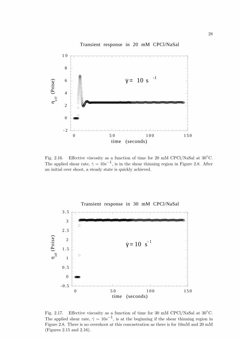
2.16 Effective viscosity as a function of time for 20 mM CPCl/NaSal at 30C.

The applied shear rate, γ = 10s−1, is in the shear thinning region in

Figure 2.8. After an initial over shoot, a steady state is quickly achieved. 28

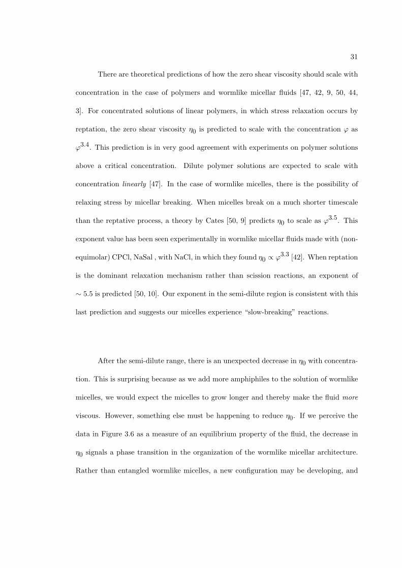
2.17 Effective viscosity as a function of time for 30 mM CPCl/NaSal at 30C.

The applied shear rate, γ = 10s−1, is at the beginning if the shear

thinning region in Figure 2.8. There is no overshoot at this concnetration

as there is for 10mM and 20 mM (Figures 2.15 and 2.16). . . . . . . . . 28

xii

2.18 Time dependent viscosity for 40 mM at 30C, at shear rate γ = 10s−1.

For shear rates near 10s−1, the viscosity of 40 mM does not change

(Figure 2.9). The shear rate is too modest to activate the non-Newtonian

properties in this experiment. . . . . . . . . . . . . . . . . . . . . . . . . 29

2.19 Zero shear viscosity versus concentration. The line passing through the

data points at 3 mM and 10 mM gives the scaling law obeyed for con-

centrations in this region, the slope of the line is ∼ 5.8, indicating that

stress is relaxed by reptation. . . . . . . . . . . . . . . . . . . . . . . . . 30

2.20 Relaxation time versus concentration. The line gives the scaling law

obeyed for concentraions from 8 mM to 65 mM: λ ∼ ϕ−4.1. . . . . . . . 32

2.21 Elastic modulus G0 versus concentration ϕ of equimolar CPCl/NaSal.

The scaling law holds for all concentrations, whereas the laws for λ and

η0 held for different concentration ranges. . . . . . . . . . . . . . . . . . 33

2.22 The “thickening frequency” or shear rate at which the fluid experiences

an increase in viscosity with increasing shear rate Data in this plot was

obtained from Figures 2.4-2.9. . . . . . . . . . . . . . . . . . . . . . . . . 35

3.1 A rising cusped air bubble in a polymer solution (0.08% carboxymethyl-

cellulose in 50:50 glycerol/water). . . . . . . . . . . . . . . . . . . . . . . 39

3.2 Cusp shape change of an oscillating bubble rising through a 15mM CPCl/NaSal

(weight fraction ϕ = 0.5%) solution at T = 37.5C. The scale at left is

marked in centimeters. Interval between pictures: 0.05 s. . . . . . . . . . 41

xiii

3.3 Height z versus time t of an oscillating bubble in 8mM CPCl/NaSal at

T= 22.4C in a 1.2 m cylinder. The data shown is 40 cm high, and 11.4

seconds in duration. VMin = 2.5cm/s, VMax = 5.2cm/s, VAve = 3.4cm/s. 43

3.4 Temperature and concentration phase diagram for the dynamics of a

rising bubbles in equimolar CPCl/NaSal, showing two distinct regions

of oscillating behavior (shaded) labelled as I and II. The straight line at

low concentrations is an isoline of equation 3.1 and marks a boundary

for type I oscillations. . . . . . . . . . . . . . . . . . . . . . . . . . . . . 48

3.5 Oscillating bubble in 30mM CPCl/NaSal at T = 21C. Interval between

pictures : 0.24 s. . . . . . . . . . . . . . . . . . . . . . . . . . . . . . . . 50

3.6 Rheology of equimolar CPCl/NaSal at T = 30C: a) effective viscosity

versus shear rate for 10, 20, 30, and 40 mM CPCl/NaSal; b) zero shear

viscosity, η0 as a function of concentration. The shaded regions mark the

concentration ranges of bubble oscillations. . . . . . . . . . . . . . . . . 51

3.7 Birefringent images of the wake behind a bubble rising in CPCl/NaSal

at T = 24C: a) 10 mM ; b) 20 mM ; c) 35 mM. Each image is 6.5 cm

high. The diameters of the bubbles are all in the range of 3 mm to 5

mm. Reynolds and Deborah numbers for each image are: a) Re ' 4.72,

De ' 250; b) Re ' 0.02, De ' 6; c) Re ' 1.1, De ' 1.8. . . . . . . . . . 55

3.8 Rising air bubble in 80 mM CPCl - 40 mM NaSal diluted in 500 mM

NaCl. The cusp is stable and no oscillations were observed. . . . . . . . 58

xiv

4.1 Effective viscosity as a function of shear rate at very low concentrations

(dilute regime). Although the viscosity decreases at higher γ, it remains

well above the η0 plateau, indicative of a thickened state. . . . . . . . . 83

4.2 Effective viscosity as a function of shear rate for a semi-dilute solution.

The increase in viscosity near is reminiscent of the thickening at lower

concentrations (Fig.4.1). . . . . . . . . . . . . . . . . . . . . . . . . . . . 84

4.3 Effective viscosity as a function of shear rate. This higher concentration

(30 mM) is no longer in the semi-dilute regime. No thickening occurs in

the range of γ tested. . . . . . . . . . . . . . . . . . . . . . . . . . . . . . 85

4.4 Schematic of micelle reactions in the 3-species model (see Table 4.1). . . 87

4.5 The effective viscosity for the 2-species model (equation 4.30) shows a

zero shear plateau at low shear rates, thinning, and then levelling off to

its asymptotic value. The zero shear viscosity and the asymptotic value

are also depicted (equations 4.31 and 4.32). Parameter choices for ηe are

M = 0.1, V = 1, ηa = 100, ηc = 0.1, k0 = 0.01, k1 = 0.06, m = 0.02,

and n = 0.007. . . . . . . . . . . . . . . . . . . . . . . . . . . . . . . . . 97

4.6 Predictions for the effective viscosity (equation 4.30), with varying flow

dependent reaction rates. Each curve is normalized by its zero shear

viscosity. Both shear thinning and shear thickening are captured by the

model. Parameter choices are M = 0.1, V = 1, ηa = 100, ηc = 0.1,

k0 = 0.01, and k1 = 0.06. . . . . . . . . . . . . . . . . . . . . . . . . . . 98

xv

4.7 Predicted normalized viscosity dependence on shear rate. Parameters

used: k0 = 1, k1 = 100, f0 = f1 = f2 = g = 100γ, ηa = 0.1, ηb = 1,

ηc = 0.01, α = β = 2. . . . . . . . . . . . . . . . . . . . . . . . . . . . . . 102

4.8 Population dynamics for long a-micelles (circles) and short c-micelles

(triangles) for Fig. 4.7 . . . . . . . . . . . . . . . . . . . . . . . . . . . . 104

4.9 Dynamics of bundle population for Fig. 4.7 . . . . . . . . . . . . . . . . 104

4.10 Predicted normalized viscosity dependence on shear rate. Parameters

used: k0 = 1, k1 = 1000, f0 = g = 100γ, f1 = 800γ, f2 = 0.01γ, ηa = 1,

ηb = 1011, ηc = 0.01, α = 0.3, β = 5.4. . . . . . . . . . . . . . . . . . . . 106

4.11 Population dynamics for a-micelles (circles) and c-micelles (triangles) for

Fig. 4.10. . . . . . . . . . . . . . . . . . . . . . . . . . . . . . . . . . . . 107

4.12 Dynamics of bundle population for Fig. 4.10. . . . . . . . . . . . . . . . 107

4.13 Predicted viscosity dependence on shear rate. Parameters used: k0 = 1,

k1 = 1000, f0 = f1 = f2 = 100γ, g = 10−6γ + 1, ηa = 0.1, ηb = 1,

ηc = 0.01, α = β = 2. . . . . . . . . . . . . . . . . . . . . . . . . . . . . . 109

4.14 Population dynamics for a-micelles (circles) and c-micelles (triangles) for

Fig. 4.13 . . . . . . . . . . . . . . . . . . . . . . . . . . . . . . . . . . . . 110

4.15 Dynamics of bundle population for Fig. 4.13 . . . . . . . . . . . . . . . 110

4.16 Predicted viscosity dependence on shear rate. Parameters used: k0 = 1,

k1 = 100, f0 = 10−6γ, f1 = 10−2γ, f2 = 100γ, g = 10−4γ, ηa = 0.1,

ηb = 1, ηc = 0.01, α = β = 2. . . . . . . . . . . . . . . . . . . . . . . . . 113

4.17 Population dynamics for a-micelles (circles) and c-micelles (triangles) for

Fig. 4.16. . . . . . . . . . . . . . . . . . . . . . . . . . . . . . . . . . . . 114

xvi

4.18 Dynamics of bundle population for 4.16. . . . . . . . . . . . . . . . . . . 114

5.1 The concentration a(t) is depicted as the dashed curve, while the solid

curve is the corrected concentration, which excludes the micelles that

grew from t1 = 3π/2 to t2 = 5π/2, and then broke by time t3 = 7π/2. . 119

5.2 The original concentration a(t) is shown as the dashed curve, while the

solid curve is a proposed replacement function for obtaining stress at

time π in equation 5.2. . . . . . . . . . . . . . . . . . . . . . . . . . . . . 121

5.3 The original concentration, a(t) is shown as the dashed curve. Here the

solid cure is the replacement function for computing stress (equation 5.2

at time 3π. . . . . . . . . . . . . . . . . . . . . . . . . . . . . . . . . . . 121

5.4 The solid curve is R a(2, t) for the concentration function depicted as the

dashed curve. . . . . . . . . . . . . . . . . . . . . . . . . . . . . . . . . . 123

5.5 The solid curve is R a(5, t) for the concentration function depicted as the

dashed curve from Figure 5.4. . . . . . . . . . . . . . . . . . . . . . . . . 123

5.6 Using the same concentration function (dashed curve) as in Figures 5.4-

5.5, the replacement function Pµ(5, t) (solid curve) correctly eliminates

the micelles destroyed from t = 1 to t = 2. For this plot we used µ = 0.02. 126

xvii

5.7 The dynamics of a-micelles is shown as the thick dashed curve. Plots of

P aµ

(0.6, t), P aµ

(1.7, t), and P aµ

(6.5, t) are also shown as solid curves, with

µ = 0.01. The paramaters used for these dynamics are the same for the

stress plots 5.10-5.14 which are: γ(t) = t, k0 = 102, k1 = 103, f0(γ) = 0,

g(γ) = 10−3γ, f1(γ) = 104γ, f2 = 106γ, α = β = 2, ηa = 103, ηb = 10,

ηc = 10−3, and λa = λb = λc = 1. . . . . . . . . . . . . . . . . . . . . . 134

5.8 The dynamics of bundles is shown as the thick dashed curve. A plot of the

modified concentration P bµ

(6.5, t) is shown as the solid curve (µ = 0.01),

which is identical to the concentration function b(t) up to that time since

b(t) is monotonically increasing. Parameter values are the same as for

Figure 5.7. . . . . . . . . . . . . . . . . . . . . . . . . . . . . . . . . . . . 134

5.9 The dynamics of c-micelles is shown as the thick dashed curve. Plots

of P cµ

(1.0, t) and P cµ

(3.0, t) are shown as solid curves, both are constant

since the concentration function c(t) is monotonically decreasing. Pa-

rameter values are the same as for Figure 5.7. . . . . . . . . . . . . . . . 135

5.10 Time dependent stress prediction using our model (equation 5.13) for

shear flow with shear rate γ(t) = t. . . . . . . . . . . . . . . . . . . . . . 137

5.11 Time dependent stress prediction of the Maxwell model for the same

shear flow used in Figure 5.10. Parameter values are the same as for

Figure 5.7. . . . . . . . . . . . . . . . . . . . . . . . . . . . . . . . . . . . 137

5.12 Time dependent stress with concentration functions inside the Maxwell

memory integral, in the same shear flow used in Figure 5.10.Parameter

values are the same as for Figure 5.7. . . . . . . . . . . . . . . . . . . . . 138

xviii

5.13 Time dependent stress with concentration functions outside the Maxwell

memory integral, in the same shear flow used in Figure 5.10. Parameter

values are the same as for Figure 5.7. . . . . . . . . . . . . . . . . . . . . 138

5.14 The logarithm (base 10) of the difference of stress values between values

from Fig. 5.10 and 5.12, as a percentage of the predicted values in Fig.

5.10 (obtained from equation 5.13). As expected, the values from Fig.

5.12 are consistently greater than those obtained from our model. . . . . 140

5.15 Model prediction (equation 5.13) for shear stress in oscillatory shear flow

plotted against time. Here γ = 0.01 cos(t), and parameter values are:

µ = 0.01, k0 = 1, k1 = 100, f0(γ) = 102|γ|, g(γ) = 10−6|γ|, f1(γ) =

10−2|γ|, f2 = 102|γ|, α = β = 2, ηa = 102, ηb = 104, ηc = 10−2, and

λa = λb = λc = 1. . . . . . . . . . . . . . . . . . . . . . . . . . . . . . . 142

5.16 Prediction of our model (equation 5.13) in oscillatory shear with shear

rate γ(t) = 0.1 cos(t). All parameter values are the same as in in Figure

5.15. With an increase in the amplitude of shear rate, a slight asymmetry

develops in the oscillating stress. . . . . . . . . . . . . . . . . . . . . . . 142

5.17 Prediction of our model (equation 5.13) in oscillatory shear flow with

γ(t) = cos(t). Parameter values are the same as those in Figures 5.15

and 5.16. At this higher amplitude oscillatory shear rate the asymmetry

is much more pronounced than in Figure 5.16. . . . . . . . . . . . . . . . 143

xix

5.18 Maxwell model prediction for shear stress in oscillatory shear flow with

shear rate γ(t) = cos(t). Values of parameters are identical to those used

in Figures 5.15-5.17. The asymmetry in Figure 5.17 (which uses the same

strain) is absent from the Maxwell prediction. . . . . . . . . . . . . . . . 143

5.19 Prediction for time dependent shear stress in oscillatory shear flow using

concentration functions on the outside of the memory integral. Here

γ(t) = cos(t) and all parameter values are the same as in Figures 5.15-5.18. 144

5.20 Prediction for time dependent shear stress in oscillatory shear flow using

the concentration functions on the inside of the memory integral. Here

γ(t) = cos(t) and all parameter values are the same as in Figures 5.15-5.19. 144

5.21 Difference of stress values between values in Figure 5.17 and 5.20 as a

percentage of the values obtained from our model prediction in Figure

5.17. The occurrence of negative value is explained in the text. . . . . . 145

5.22 Time dependent shear stress prediction of our model equation 5.13 in a

thixotropic loop. Parameter values used are: µ = 0.01, k0 = 102, k1 =

103, f0(γ) = 0, g(γ) = 10−3γ, f1(γ) = 104γ, f2 = 106γ, α = β = 2,

ηa = 103, ηb = 10, ηc = 10−3, and λa = λb = λc = 1. Stress values

obtained while γ is increasing are given as squares, the triangles denote

stress values when the shear rate is decreasing. . . . . . . . . . . . . . . 148

xx

5.23 Maxwell model prediction for shear stress in a thixotropic loop using the

same time dependent shear rate as in Figure 5.22. All paramter values

used to obtain the values in this plot are the same as in Figure 5.22.

The Maxwell model predicts a much greater shear thickening effect than

our model (equation 5.13) shown in Figure 5.22. Stress values obtained

while γ is increasing are given as squares, the triangles denote stress

values when the shear rate is decreasing. . . . . . . . . . . . . . . . . . . 148

5.24 Prediction of shear stress in a thixotropic loop using the concentration

functions outside the memeory integral. The shear rate and all parameter

values used are the same as those used to produce the values in Figure

5.22 and 5.23. Stress values obtained while γ is increasing are given as

squares, the triangles denote stress values when the shear rate is decreasing. 149

5.25 Predicted shear stress values in a thixotropic loop study. The shear rate

and all parameter values used are the same as those used to produce the

values in Figure 5.22-5.24.Stress values obtained while γ is increasing are

given as squares, the triangles denote stress values when the shear rate

is decreasing. . . . . . . . . . . . . . . . . . . . . . . . . . . . . . . . . . 149

5.26 Logarithm (base 10) of the precent difference of stress values obtained

from Figure 5.24 and 5.22, plotted against shear rate. The squares again-

denote stress values obtained using shear rate values when the rate is

increasing, while triangles are obtained by using shear rates when γ(t) is

decreasing - consistent with thier use in Figures 5.22-5.25. . . . . . . . . 150

xxi

Acknowledgments

During my graduate studies, it has been a joy to work among the undergradu-

ates, graduates, post-docs, and professors associated with the Pritchard Lab. My thesis

advisor, Andrew Belmonte, created an atmosphere of cooperation and friendship in the

lab, which encouraged our interest in our studies and helped us dismiss our intellectual

insecurities. Learning from one another was unavoidable. I enjoyed and benefited from

many discussions with Josh Gladden, Mike Sostarecz, Yuliya Gorb, Jon Jacobsen, Bob

Geist, Linda Smolka, Austin Semerad, Young-Ju Lee, Anand Jayaraman, Thomas Pod-

gorski, Ben Akers, Diane Henderson, Anna Mazzucato, Francesco Costanzo, and Andrew

Belmonte.

I began working with Andrew after a very disappointing period of graduate work

in geometry. His dedication to my education and the value he gave my ideas helped me

to recover and grow. It has been my privilege to study with him, and I have enjoyed our

collaborations. I must also thank the Belmonte family for their warm friendship while

graciously tolerating so many late night visits to meet with Andrew. Let me also say

thanks for feeding an always hungry graduate student.

Many seminar speakers our lab hosted, as well as people I met at conferences, took

time to listen to my experimental and theoretical work. I am inspired by their interest

and grateful for their advice and insight. My sincere thanks to Eric Weeks, Bob Leheny,

Peter Olmsted, Elisha Moses, Ralph Colby, Ranjini Bandyopadhyay, Jim Keener, Lynn

Walker, and Stephen Childres.

xxii

In addition to my studies and research, my graduate duties included teaching and

copious paperwork for which I was born with an inclination to avoid. Unfortunately,

paperwork usually comes equipped with deadlines, and this poses a serious threat to me.

I want to thank the excellent staff in the Mathematics Department, especially Becky

Halpenny, for taking care of things and creating the illusion I live with that “things just

work themselves out”.

I thank my friends Sumant, Stephan, Susan, and my dear friend Paul. My brother

Damian and his wife Renia have often made my life easier by “making things work

themselves out” as well, freeing me to concentrate on my thesis. Their efforts are much

appreciated as is thier love.

Most of all I thank my parents. The love and support my mother and father gave

me directly impacts my work and my life. It is because of their guidance and care that

I have completed my graduate degree. They have my undying love.

1

Chapter 1

Introduction

Imagine holding a pole in the middle of a flowing river. The force you need to

apply to keep the pole upright is a measure of the viscous drag exerted by the river.

Intuition would tell you that the faster the river is flowing, the harder it would be to

keep the pole straight, and after a few minutes you might have a good feel for how much

force the river is exerting. Now suppose that all of a sudden you feel the river pushing

much harder, even though it is not going any faster! Such an unexpected surprise could

find you asking: What is this river made of? The answer would be a fluid made of tiny

objects no bigger than the thickness of a human hair, a wormlike micellar fluid.

This Thesis begins by showing some of the extraordinary behavior of wormlike

micellar fluids, in experiments not so different from the one just described. In highly

controlled situations, the fluid speed can be increased in small increments, and very

precise values of viscous drag (or stress) are recorded. This is the study of rheology, and

in Chapter 2 we show our rheological data after first describing wormlike micellar fluids.

Chapter 3 continues with experimental results, studying the behavior of the fluid

in a more complicated flow. Specifically, we examine the fluid’s response to a constant

stress imposed by the buoyancy of a rising air bubble. To place the results in context we

review aspects of rising bubbles in other liquids, including water and polymer solutions.

The behavior of rising bubbles is studied as a function of the concentration of wormlike

2

micelles in the fluid, and the bubble behavior is able to sense a phase transition in the

fluid microstructure as concentration increases past a certain threshold. These results

are combined with the rheology presented in Chapter 2 to provide a more comprehensive

understanding of the phase transition.

The understanding we develop from the experimental observations (our own and

from published sources) presented in Chapters 2 and 3, helps us to describe the physical

processes taking place inside the fluid which bring about the effects we see. To formalize

such a description, in Chapter 4 we focus on the physical properties we consider most

relevant to the effects seen experimentally, and present these processes mathematically.

Using three coupled ordinary differential equations to describe interactions taking place

among the micelles, we write a model for the stress developed in the fluid during steady

state (time independent) flow. Simulated results are then studied and compared to the

rheological results presented in Chapter 2.

Chapter 5 then pursues a description of fluid flow in the more generic case of

time dependent flows. The physical ideas that led to the mathematics in Chapter 4 are

re-examined, and we find that the time dependent case requires a more sophisticated

mathematical approach. We then write the time dependent model explicitly, and study

how it works in the case of three different types of flow. The results are compared to

similar mathematical equations which we argue are physically inaccurate.

Chapter 5 is concluded with a very interesting connection between our model

and the Fredholm theory of integral equations. We provide results about our model

which show it to be amenable to the powerful techniques of this theory. The possible

3

answers Fredholm theory could provide about our model are discussed and their physical

relevance to known rheological results on wormlike micellar fluids.

4

Chapter 2

Rheology and Microscale Architecture

of Wormlike Micellar Fluids

This chapter is an introduction to wormlike micellar fluids. These fluids are

viscoelastic and form a very interesting subset of non-Newtonian fluids. We start with

a description of how wormlike micelles are formed, their approximate size, and the role

of the different molecules involved in their formation. We then present our results from

numerous rheological tests on certain wormlike micellar systems, and explain what the

data says about the particular system we are studying, and how it relates to known

rheological results.

2.1 Chemistry and self-assembly

Wormlike micelles are an example of what are called “self-assembling” structures.

A micelle is not a molecule, it consists of molecules which have the ability to come

together in aqueous solution to form the micelle. In our experiments we have used a

specific set of molecules to make wormlike micellar fluids, and we begin by describing

the self assembling process of this particular choice of chemicals. Once the process is

explained, it will be easier to discuss how general this process is and other ways wormlike

micellar fluids are made.

The fluids used in our experimental studies were made of three raw components:

CetylPyridiniumChloride (CPCl), Sodium Salicylate (NaSal), and deionized water. The

5

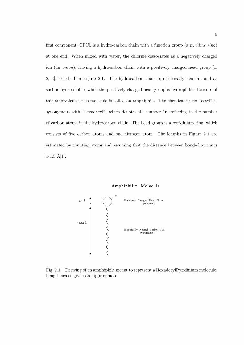
first component, CPCl, is a hydro-carbon chain with a function group (a pyridine ring)

at one end. When mixed with water, the chlorine dissociates as a negatively charged

ion (an anion), leaving a hydrocarbon chain with a positively charged head group [1,

2, 3], sketched in Figure 2.1. The hydrocarbon chain is electrically neutral, and as

such is hydrophobic, while the positively charged head group is hydrophilic. Because of

this ambivalence, this molecule is called an amphiphile. The chemical prefix “cetyl” is

synonymous with “hexadecyl”, which denotes the number 16, referring to the number

of carbon atoms in the hydrocarbon chain. The head group is a pyridinium ring, which

consists of five carbon atoms and one nitrogen atom. The lengths in Figure 2.1 are

estimated by counting atoms and assuming that the distance between bonded atoms is

1-1.5 A[1].

Positively Charged Head Group (hydrophilic)

+

Electrically Neutral Carbon Tail (hydrophobic)

Amphiphilic Molecule

4-5 A

14-16 A

Fig. 2.1. Drawing of an amphiphile meant to represent a HexadecylPyridinium molecule.Length scales given are approximate.

6

These amphiphilic molecules are sometimes called surfactants. This word is used

because when the amphiphile (surfactant) is in water, it goes to the surface to enable the

hydrophobic carbon tail to escape from the water, leaving the hydrophilic head to remain

in contact with the water. This in turn reduces the surface tension of the liquid. The

point is that the molecule (more correctly the surrounding water) always prefers to have

hydrophobic tail excluded from the water. When a critical concentration of amphiphiles

is reached, another way of excluding or hiding the tails from the water is available. The

molecules can gather together in such a way that the surrounding water does not come

in contact with the tails, and only interacts with the head groups. For example, this

would be achieved if the molecules aggregated into spheres with the heads on the surface

of the sphere, and all tails pointing towards the center as in Figure 2.2.

Spherical Micelle

Fig. 2.2. A spherical micelle. Hydrophilic heads form the surface of the sphere, whilehydrocarbon tails fill the interior

7

This is our first example of a micelle, in this case a spherical micelle, and the

aggregation process is called micellization. The critical concentration of amphiphiles

needed for micellization to occur is called the critical micelle concentration or CMC [2].

The diameter of a spherical micelle would be roughly twice the tail length ∼ 20− 30 A.

Even above the CMC, there is a fixed concentration (equal to the CMC) of amphiphiles

which exist individually in solution, not in a micelle.

Micellization occurs in order to raise the entropy of the surrounding water, thereby

reducing the free energy of the system. However, there are competing forces in micelle,

which push the amphiphiles away from each other when they come too close together.

Since the head groups are positively charged, there is a Coulomb (electrostatic) repulsion

pushing them away from each other. There is also the crowding of the carbon tails

inside the sphere, which lowers their entropy and prevents too many amphiphiles from

occupying a single spherical micelle [2, 5].

This brings us to the second of the three components we listed above, namely

the organic salt NaSal. Dissolved in water, the salt molecule NaSal seperates into Na+

and a salicylate molecule Sal−, which itself has a hydrophobic part to it. If NaSal is

added to a fluid consisting of spherical micelles made from CPCl, the Sal− prefers to

obscure its hydrophobic portion by penetrating into the spherical micelle [2, 4, 5, 6]. It

therefore can serve to screen the Coulomb repulsion of the positively charged head groups

of the amphiphiles. The effect of introducing the Sal− on the geometry of the micelle

is a transition from spherical to rod-like or cylindrical micelles [5, 7, 8]. The cylindrical

micelles terminate at ends which are hemi-spherical, as if the cylinder grew from the

sphere by cutting the sphere into two equal halves and adding a cylinder between them.

8

The sketch in Figure 2.3 shows how the amphiphiles are arranged in the cylin-

drical portion and hemi-spherical endcaps, with approximate length scales. It must be

understood that the rendition in Figure 2.3 is speculation, though the length scales

have been approximated experimentally [3, 9]. The lengths of wormlike micelles can

range from nanometers to microns. The average length of wormlike micelles depends on

factors such as total amphiphile concentration, temperature, and concentration of salt.

Furthermore, the distribution of lengths in a wormlike micellar fluid can be highly dis-

perse [2, 4, 5, 7]. At concentrations sufficiently greater than the CMC, and with enough

salt, the wormlike micelles are long and flexible, resembling something like a worm. The

lengths that wormlike micelles can achieve, together with their flexibility, make them

similar to polymer chains [6]. And like polymer solutions, wormlike micellar fluids are

viscoelastic non-Newtonian fluids.

4nm

100nm - 1µm

Hemi-SphericalEndcap

Fig. 2.3. A cylindrical or wormlike micelle. The micelle terminates in a hemi-sphericalendcap in which amphiphiles may be organized as in a shperical micelle. Length scalesare estimateed from experimental data on womrlike micelles [9, 10]

9

It is important, though, to remember that the micelles are not molecules, and

that there are no chemical bonds between neighboring amphiphiles and organic salt

molecules as there are in polymer chains. The micelles form due to the hydrophobic

effect, and can both break into smaller micelles, or join with other micelles to form

a longer micelle, under the influence of thermal fluctuations. These kinetic reactions

constantly occur in the fluid, even in equilibrium, and individual amphiphiles are also

free to leave a given micelle, enter a new micelle or join the pool of free amphiphiles. In

equilibrium these processes are of course in balance with one another. A well accepted

model for the average length of wormlike micelles [9, 2, 4] in equilibrium predicts that the

average length of micelles, L0, scales with amphiphile concentration ϕ and temperature

T according to the relation:

L0 ∼√

ϕeE/2kT . (2.1)

The constant k is Boltzmann’s constant: k ' 1.4×10−23 Joules/Kelvin. In the exponent,

the E is the energy needed to hold a micelle together, analogous to the bond energy of

a molecule. This “bond” energy is equated with the energy needed to break a micelle

into two micelles, and called the scission or endcap energy. The reason is that it is

thought that the the “bond energy” is due to the high curvature and dense packing

of hydrophobic tails in the hemi-spherical endcaps. The linear cylindrical portion is

believed to have little or no energy cost. Under this assumption, breaking a micelle into

two micelles requires the creation of two hemispherical endcaps, which requires a cost of

energy equal to the “bond energy” of the micelle. Thus the notions of endcap energy,

scission energy, and “bond” energy are identical to one another.

10

The scaling in equation 2.1 is strictly in equilibrium, and in its derivation it is

assumed that there are no interactions among the wormlike micelles [5, 9]. It makes the

most sense, therefore, to use this model in dilute, or perhaps semi-dilute, solutions in

which micelles are on average far enough apart from one another to avoid interactions.

It is likely that motion of the fluid changes the length distribution, and while it is not

known what the non-equilibrium lengths are, predictive models have been hypothesized.

In Chapter 4 we review some of these models and the relevance of their predictions to

experimental rheology.

2.1.1 Alternative chemical components

The description of the self-assembly of amphiphiles (surfactants) into micelles

given in section 2.1 is somewhat generic, not particular to wormlike micelles made from

CPCl and NaSal. Other surfactants that can lead to wormlike micelles in the way we

have described as well [3, 9, 11]. A selection of such surfactants that are commonly found

in experimental literature are listed here: Cetyltrimethylammonium Chloride (CTAB),

Cetyltrimethylammonium Tosylate (CTAT), and tris(2-hydroxyethyl)-tallowalkyl ammo-

nium acetate (TTAA). Each surfactant can be combined with the organic salt Sodium

Tosylate (NaTos), or NaSal [12]. Other non-organic salts sometimes used in addition to

an organic salt include Potassium Bromide (KBr), Sodium Bromide (NaBr), and Sodium

Chloride (NaCl). The organic salts facilitate growth of wormlike micelles because of their

hydrophic carbon chains, which pentrate into the micelle to avoid interactions with the

polar water molecules [2]. Inorganic salts such as KBr, when used with an organic salt,

11

have little or no effect as a catalyst for the sphere to rod transition and subsequent

growth to long, flexible wormlike micelles [7, 9].

Each choice of surfactant and salt will produce micelles with different length

distributions, different degrees of viscosity and elasticity. For a single surfactant, the

amount of salt used can dramatically affect the size distribution as well the rheological

properties of the fluid [9, 5, 6, 8]. For our experiments, we have chosen the combination

of CPCl with organic salt NaSal, and we use them in equal parts (with the exception of

certain experimental results in Chapter 3, where the precise combination is stated). The

NaSal acts a particularly effective counterion, and using equal parts of surfactant and

salt gives us a maximal growth rate of wormlike micelle for the concentration ranges we

use [6].

2.2 Steady shear rheology

Incompressible viscous Newtonian fluids can be characterized mathematically as

those fluids which obey the Navier-Stokes equation

%∂u∂t

+ % (u · ∇)u = −∇p + η∇2u,

in which % is the fluid density, η the viscosity, p is pressure, and u the velocity. For fluids

of constant density there is a single material parameter, η, and for Newtonian fluids it is

not a function of u. Indeed, Newtonian fluids are those for which the stress σ is linearly

related to velocity gradients, with proportionality constant η: σ = η(∇u +∇uT ).

12

Viscoelastic non-Newtonian fluids have more complex material properties in the

sense that they are elastic and their viscosity can depend on the flow. In this section we

examine the material properties of wormlike micellar fluids in motion, specifically in sim-

ple shear flow. In Cartesian coordinates (x1, x2, x3), simple shear flow is a velocity field

u such that u has only one non-zero component, and ∇u has one non-zero component

which is constant in space and orthogonal to the direction of u. Thus if u = (u1, 0, 0),

then

∇u =

0 0 0

γ 0 0

0 0 0

,

in which γ = ∂u2∂x1

. Here, γ is called the shear rate and is spatially constant, but can

depend on time.

The study of the material properties of fluids in shear flow is the subject of shear

rheology [47, 83]. Shear flow is one of two flow types considered in rheology, the other

being extensional flow in which all velocity gradients are parallel to the direction of flow.

Rheology is performed with a rheometer, and we describe now the rheometer we have

used for the data presented here. In shear rheology a fluid sample is loaded into a chamber

which is confined to shearing motion. There are then two possible ways to control the

motion: through applied stress or applied strain rate. In a stress controlled rheometer, a

force of the controller’s design is applied to the walls of the chamber containg the fluid,

inducing shear flow. The rheometer then measures the shear rate and reports this value.

Factors such as duration of measurement, temperature of chamber, and duration of flow

13

before measurement begins are adjustable parameters and can effect the reported values.

In controlled strain rate rheology, a shear rate is applied, and the shear stress is reported.

For all data in this Thesis, we have used a controlled rate of strain rheometer 1, with

circulating temperature bath to control the temperature of the chamber containing the

fluid sample, in a stainless steel Couette geometry.

The data in Figures 2.4-2.9 are “steady shear rate sweep tests.” In these tests,

a constant shear rate is applied to the fluid for as much as 45-500 seconds (called the

delay time), after which the stress is measured for 45-90 seconds (called the measurement

time). The stress having been recorded, the shear rate is increased to a higher constant

value and the measurement is again taken. This procedure is repeated up to a final shear

rate γf which varies slightly for each fluid tested. The fluids used for these experiments

are equimolar concentrations of CPCl and NaSal. (Procedures used to make these fluids

are discussed fully in Chapter 3). The concentrations used vary from 1 mM to 65 mM,

and the exact concentrations used are given in Figures 2.4-2.9. A delay time was chosen

for each concentration based on how long it takes to achieve a steady state stress value

for that concentration. All tests reported here were performed at 30Celsius, accurate

to within 1.0C.

In Figure 2.4, the concentrations used were 1 mM, 2 mM, and 3 mM CPCl/NaSal.

In the data for 1 mM, we start at the smallest rates γ and work our way up. Then the

plot begins with a constant viscosity value for γ ∼ 10s−1 to 30s−1 called the zero-shear

1Rheometrics RFS III with transducer model 100 FRT, Rheometric Scientific is now ownedand operated by TA Instruments, New Castle, Delaware.

14

0 . 0 0 1

0 . 0 1

0 . 1

1

1 0 1 0 0 1 0 0 0

1 mM2 mM3 mM

η eff

(P

oise

)

Shear rate (s- 1)

Effective Viscosity - Shear Thickening

Fig. 2.4. Steady state effective viscosity as a function of shear rate for 1 mM, 2 mM,and 3 mM CPCl/NaSal at 30C.

0 . 0 1

0 . 1

1

1 1 0 1 0 0 1 0 0 0

3.4 mM3.7 mM4 mM

η eff

(P

oise

)

Shear rate (s- 1)

Effective Viscosity - Shear Thickening

Fig. 2.5. Steady state effective viscosity as a function of shear rate for 3.4 mM, 3.7 mM,and 4 mM CPCl/NaSal at 30C.

15

viscosity η0. For 1 mM η0 ∼ 0.01 Poise, which is roughly the viscosity of water, which

means in equilibrium, the fluid seems Newtonian, and there is no evidence that there are

micelles in the fluid. Near γ ∼ 30s−1 however, the viscosity rapidly increases to a value

which is an order of magnitude greater, showing the fluid is certainly non-Newtonian. So

the solution became “thicker” above some critical shear rate γcrit ∼ 30s−1. Clearly then

this fluid is not Newtonian. In fact, this same type of thickening transition is observed

for 2 mM - 4 mM in Figures 2.4 and 2.5.

What we are observing is called “shear thickening”, and is an interesting phe-

nomenon in low viscosity (or dilute) wormlike micellar fluids. In an outstanding ex-

periment, C. Liu and D. Pine [17] observed such thickening in their rheology of dilute

solutions of wormlike micellar fluids made from CTAB/NaSal and performed additional

light scattering experiments to determine length scales of the micelles. What they found

was that the sizes observed were not consistent with wormlike micelles. Rather, they

likened the observed structures to a rope consisting of coiled threads (presumably the

wormlike micelles), so that the micelles “banded” together to form a new larger struc-

ture. This structure has received much attention [35, 38, 39, 40, 84] and has come to be

known as a “shear induced structure” or SIS. The rheology shown in Figures 2.4 and 2.5

are a likely indication of SIS formation in these concentrations. There are two things

to notice about the SIS formation in these Figures: the shear rate at which they begin,

and the zero-shear viscosity of the fluid. Although we will have much more to say about

these quantities in section 2.4, we note that all η0 are within an order of magnitude of

the viscosity of water, and the critical shear rate for thickening is decreasing as concen-

tration increases. We also note that the thickening jump, ηmax − η0 (where ηmax is

16

the maximum viscosity), is decreasing with concentration, and in fact ηmax seems to

plateau.

Increasing concentration further to 6 mM, we see that the shear thickening is

replaced with a decrease in viscosity from the zero shear plateau (Figure 2.6). Fluid

which display a decrease in viscosity with increasing shear rate, like the fluids in Figure

2.6, are called “shear thinning” fluids. Shear thinning in polymer solutions is thought

to happen because polymers become aligned in the direction of flow by the orthogonal

velocity gradient. Aligned in this way, the polymers would transfer less momentum to

their neighbors, resulting in a decreased viscosity. For wormlike micelles, which can

break and reform, thinning could be due to alignment or, possibly, to a decreased size

of micelle from breaking.

Note also that the η0 values for 6 mM, 7 mm, 8 mM, and 9 mM are much higher

than those for the dilute solutions of Figures 2.4 and 2.5. For 6 mM-9 mM, zero shear

viscosities range from 1 to ∼10 Poise, which is 2-3 orders of magnitude greater than the

η0 values for 1-4 mM. So there is a tremendous increase in η0 coincident with the shift

from shear thickening to shear thinning . That these changes occur over such a modest

increase in concentration is poignant. Indeed, by increasing the concentration from 1

mM or 2 mM CPCl to 3 mM or 4 mM, we produce no significant qualitative difference,

but increasing from 4 mM to 6 mM we introduce an entirely new behavior.

Yet at higher shear rates there is an increase in viscosity reminiscent of shear

thickening. It is difficult to see the precise values of viscosity at shear rates γ ∼ 100s−1

17

0 . 0 1

0 . 1

1

1 0

1 0 0

0 . 0 1 0 . 1 1 1 0 1 0 0 1 0 0 0

6 mM7 mM8 mM9 mM

η eff

(P

oise

)

Shear rate (s- 1)

Effective Viscosity - Shear Thinning

Fig. 2.6. Steady state effective viscosity as a function of shear rate for 6 mM, 7 mM, 8mM, and 9 mM CPCl/NaSal at 30C. After shear thinning, each concentration displaysa viscosity increase at high shear rate, shown more clearly in Figure 2.7.

0 . 1

1

1 0

0 . 0 1 0 . 1 1 1 0 1 0 0 1 0 0 0

7 mM

η eff

(P

oise

)

Shear rate (s- 1)

Effective Viscosity

Fig. 2.7. Effective viscosity of 7 mM CPCl/NaSal at 30C. Shown by itself, thethickening at γ ∼ 50s−1 is more visible. The increase in viscosity from γ = 40s−1 toγ = 100s−1, is similar to the thickening increase for the low concentration solutions inFigure 2.5.

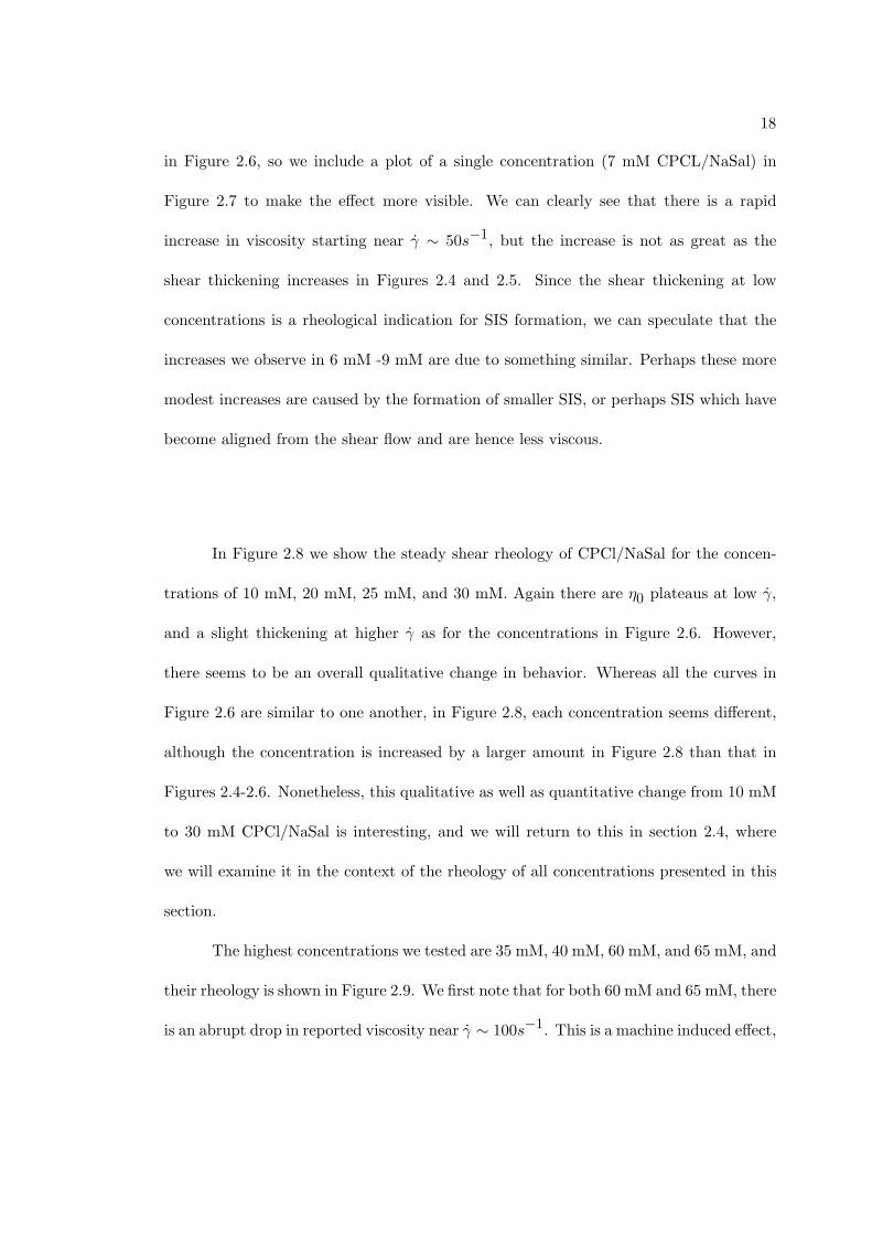
18

in Figure 2.6, so we include a plot of a single concentration (7 mM CPCL/NaSal) in

Figure 2.7 to make the effect more visible. We can clearly see that there is a rapid

increase in viscosity starting near γ ∼ 50s−1, but the increase is not as great as the

shear thickening increases in Figures 2.4 and 2.5. Since the shear thickening at low

concentrations is a rheological indication for SIS formation, we can speculate that the

increases we observe in 6 mM -9 mM are due to something similar. Perhaps these more

modest increases are caused by the formation of smaller SIS, or perhaps SIS which have

become aligned from the shear flow and are hence less viscous.

In Figure 2.8 we show the steady shear rheology of CPCl/NaSal for the concen-

trations of 10 mM, 20 mM, 25 mM, and 30 mM. Again there are η0 plateaus at low γ,

and a slight thickening at higher γ as for the concentrations in Figure 2.6. However,

there seems to be an overall qualitative change in behavior. Whereas all the curves in

Figure 2.6 are similar to one another, in Figure 2.8, each concentration seems different,

although the concentration is increased by a larger amount in Figure 2.8 than that in

Figures 2.4-2.6. Nonetheless, this qualitative as well as quantitative change from 10 mM

to 30 mM CPCl/NaSal is interesting, and we will return to this in section 2.4, where

we will examine it in the context of the rheology of all concentrations presented in this

section.

The highest concentrations we tested are 35 mM, 40 mM, 60 mM, and 65 mM, and

their rheology is shown in Figure 2.9. We first note that for both 60 mM and 65 mM, there

is an abrupt drop in reported viscosity near γ ∼ 100s−1. This is a machine induced effect,

19

0 . 1

1

1 0

1 0 0

0 . 0 1 0 . 1 1 1 0 1 0 0 1 0 0 0

10 mM20 mM25 mM30 mM

η eff

(P

oise

)

Shear rate (s- 1)

Effective Viscosity - Shear Thining

Fig. 2.8. Steady state effective viscosity as a function of shear rate for 10 mM, 20 mM,25 mM, and 30 mM CPCl/NaSal at 30C.

0 . 1

1

1 0

0 . 1 1 1 0 1 0 0 1 0 0 0

35 mM40 mM60 mM65 mM

η eff

(P

oise

)

Shear rate (s- 1)

Effective Viscosity

Fig. 2.9. Effective viscosity of 35 mM, 40 mM, 60 mM, and 65 mM CPCl/NaSal at 30C.The apparent discontinuous drop in viscosity for 60 mM and 65 mM is a spurious resultdue to a switch from one transducer to a stronger transducer, which is an automaticresponse due to an overload of torque. This is addressed more fully in the text.

20

meaning the reported values for viscosity were adjusted by an “offset value” starting

precisely at γ = 158s−1 for both 60 mM and 65 mM. The rheometer design is such

that if measured stresses are 80 − 100% of a threshold stress, the machine begins to

record stress with an alternate transducer, right in the middle of the experiment. This

transducer switch is recorded by the rheometer, but the exact offset value is not. While

the offset amount could be estimated, we have chosen to present the raw data because

it is honest and we feel it is an important example of machine induced error. This

does happen in experimental science and acknowledging it is important so that one can

remain wary of spurious effects and identify false data. We can however estimate the

offset value based on calibration parameters for both 60 mM and 65 mM, and we find

that the corrected viscosity values place the data points in Figure 2.9 in line with the

rest of the data for those concentrations.

We observed that the curves for the concentrations in Figure 2.8 were qualitatively

different from each other, and we see that in Figure 2.9 the rheology of 35 mM up to

65 mM all look very similar in terms of zero shear viscosity. Furthermore, they all have

a broad range of shear rates over which they maintain their zero shear plateaus, much

broader than concentrations as low as 6 mM and as high as 20 mM. In addition, there

is no longer a thickening at high γ as there is for each concentration in Figures 2.6 and

2.8.

Although SIS formation is typically associated with, and has been directly ob-

served in, low concentration wormlike micellar fluids [38, 39], there is evidence that

these structures can form at higher concentrations as well. In the same wormlike micel-

lar fluid we use, Wheeler et al. [40] observe SIS formation in equimolar solution of 40

21

mM CPCl/NaSal. While we do not observe any thickening region in our data for 40 mM

in Figure 2.9, it is likely that it is because our experiments are done at 30C, while those

in [40] are performed in the range 19−22C. In fact, we have tested 40 mM CPCl/NaSal

at 20C, and found a thickening region near γ ∼ 60s−1. So even though fluids in the

concentration range 6 mM -30 mM shear thin before they thicken, it is our belief that

SIS form in these fluids as well. In section 2.3, we explore the time dependent rheology

during SIS formation in our low concentration fluids, which will provide more evidence

that the shear thickening we observe in 6 mM -30 mM is a sign of SIS formation.

2.3 Transient shear rheology

The data presented here in Figures 2.10-2.18 represents the results of transient

stress measurements (with the same rheometer and Couette geometry). In each test, a

shear rate is chosen and held fixed, the rate is applied and the resulting stress is recorded

as a function of time. In this way we can gain information about the individual data

points in each of the plots shown in section 2.2. That is to say, by looking at what the

viscosity values are before they reach steady state, we may be able to deduce something

about the micellar interactions or the stability of SIS for example.

The steady state rheology of 1 mM CPCl/NaSal shown in Figure 2.4 shows two

behaviors: zero shear plateau and shear thickened region. Figures 2.10 and 2.11 show

the time dependent viscosity at shear rates in each of these regions. At γ = 25s−1, the

viscosity of 1 mM is still equal to η0, which means the fluid is nearly in equilibrium,

22

-0 .002

0

0 . 0 0 2

0 . 0 0 4

0 . 0 0 6

0 . 0 0 8

0 . 0 1

0 1 0 0 2 0 0 3 0 0 4 0 0 5 0 0 6 0 0 7 0 0

η eff (

Poi

se)

time (seconds)

Transient response in 1 mM CPCl/NaSal

γ = 25 s- 1.

Fig. 2.10. Effective viscosity as a function of time for 1 mM CPCl/NaSal at 30C. Theapplied shear rate, γ = 25s−1, is in the zero shear viscosity plateau in Figure 2.4.

0

0 . 5

1

1 . 5

2

2 . 5

3

0 1 0 0 2 0 0 3 0 0 4 0 0 5 0 0

stre

ss

(d

yne/

cm2)

time (seconds)

1 mM CPCl/NaSal at T = 30 Celsius

γ = 40 s- 1.

Fig. 2.11. Effective viscosity as a function of time for 1 mM CPCl/NaSal at 30C.The applied shear rate, γ = 40s−1, is in the thickening region in Figure 2.4. The longtransient lasting more than 200 seconds could easily be mistaken for a steady state value.

23

so it is not surprising that the time dependent viscosity quickly achieves a steady state

value. The shear thickening for 1 mM CPCl/NaSal begins near γ = 30s−1, so for

shear rates above that, the fluid is far from equilibrium and we could hope to see the

structure formation reflected in the transient response. Figure 2.11 is the transient stress

at γ = 40s−1, in which the stress is constant for roughly 250 seconds, which could easily

be thought to be the steady value. However, the stress begins to dramatically increase

by more than an order of magnitude, whereupon the stress begins to fluctuate. After

400 seconds, it is not easy to judge whether a steady state has been achieved. This time

dependent behavior is consistent with the time dependent observations in [17] in which

the inhomogenous SIS formation is certain [17, 39].

The same type of transient rheology occurs for 2 mM, where again we believe

SIS develop during flow with rates above γ ∼ 25s−1. In Figure 2.12 we show two time

dependent responses at shear rates γ = 27s−1, 40s−1 in the thickening region. Here we

see that at γ = 27s−1, which gives a viscosity less than the maximum in Figure 2.4, the

viscosity rises more slowly than at γ = 40s−1, which is a rate firmly in the thickened

region. The thickening occurs more quickly at γ = 40s−1 than at 27s−1. The shear rates

at which shear thickening begins in fact has an interesting dependence on concentration,

and we will address this in more detail in section 2.4.

The steady rheology for 6 mM in Figure 2.6 shows that this fluid begins to thicken

near γ ∼ 45s−1, at higher γ for which the fluid has shear thinned. The transient rheology

for 6 mM at γ = 50s−1 is shown in Figure 2.13. The inception time for the rise in viscosity

24

-0 .02

0

0 . 0 2

0 . 0 4

0 . 0 6

0 . 0 8

0 . 1

0 1 0 0 2 0 0 3 0 0 4 0 0 5 0 0 6 0 0 7 0 0 8 0 0

ηef

f (P

oise

)

time (seconds)

γ= 27 s- 1.

γ = 40 s- 1.

Transient response in 2 mM CPCl/NaSal

Fig. 2.12. Effective viscosity as a function of time for 2 mM CPCl/NaSal, at 30C,at two different shear rates. Both shear rates are in the thickening region for 2 mM inFigure 2.4. Like 1 mM in Figure 2.11, at γ = 27s−1 there is a long transient whichappears as a constant, almost steady state value. At γ = 40s−1, the inception time forthickening is less than 100 seconds. Both rates produce fluctuating viscosities (stresses).

-0 .05

0

0 . 0 5

0 . 1

0 . 1 5

0 . 2

0 . 2 5

0 . 3

0 5 0 1 0 0 1 5 0 2 0 0 2 5 0 3 0 0 3 5 0

η eff (

Poi

se)

time (seconds)

γ = 50 s- 1.

Transient response in 6 mM CPCl/NaSal

Fig. 2.13. Effective viscosity as a function of time for 6 mM CPCl/NaSal at 30C.The applied shear rate, γ = 50s−1, is in the thickening region in Figure 2.6. The longinception times of 1 mM and 2 mM are not copied by 6 mM, however there is a roughlyconstant viscosity of 0.1 after the intial overshoot, lasting roughly 50 seconds. Theviscosity for 6 mM fluctuates more wildly than for the lower concentrations.

25

to occur is approximately 50 seconds, much shorter than the 250 seconds needed for the

SIS development in 1 and 2 mM (see Figures 2.10 and 2.12). However, at the higher shear

rate of 40s−1, the inception time was less than 100 seconds in 2 mM. Furthermore, the

time dependent rheology for 6 mM shows large fluctuations in viscosity once thickening

has occured, as do 1 mM and 2 mM. The larger fluctuations and shorter inception time

are probably because the shear rate at which thickening occurs is higher in 6 mM than

at the lower concentrations. Note that these fluctuations do not occur at γ = 25s−1 in

1 mM, and thickening is not observed in this fluid (Figure 2.10).

To check if such fluctuations are specific to the thickening shear rate range, we

tested 8 mM at two shear rates (Figure 2.14): γ = 12s−1 which is in the thinning

region, and γ = 60s−1 which is in the thickening region. At a shear rate of γ = 12s−1,

the viscosity quickly achieves its steady value, and remains relatively constant. At γ =

60s−1, the fluctuations are clearly evident, however there is no longer an appreciable

inception time for viscosity growth. The inception time may be reduced because of the

higher shear rates, which could speed the reactions necessary to for the SIS.

The loss of an incepetion time creates doubt that the shear thickening in 6 mM-

35 mM coincides with structure formation. While it seems that, in dilute solutions, an

inception time on the order of hundreds of seconds is typical in SIS formation [17, 84], we

do observe that the inception time decreases from 1 mM to 4 mM CPCl/NaSal (Figures

2.4 and 2.5). It may simply be that the time needed to form SIS is reduced at higher

concentrations because the fluid begins with larger wormlike micelles, making it easier

to form the induced structures.

26

- 0 . 2

0

0 . 2

0 . 4

0 . 6

0 . 8

0 5 0 0 1 0 0 0 1 5 0 0 2 0 0 0

η eff

(P

oise

)

time (seconds)

γ = 12 s - 1.

γ = 60 s- 1.

Transient response in 8 mM CPCL/NaSal

Fig. 2.14. Effective viscosity as a function of time for 8 mM CPCl/NaSal, at 30C, attwo different ahear rates. The lower shear rate, γ = 12s−1 is in the thinning reagion (seeFigure 2.6). The higher rate, γ = 60s−1, is at the very beginning of the shear thickeningregion for 8 mM. At γ = 60s−1, time dependent rheology shows fluctuating viscosity,though there is no evident inception time for the thickening to begin.

- 0 . 5

0

0 . 5

1

1 . 5

2

2 . 5

0 5 0 1 0 0 1 5 0

ηef

f (P

oise

)

time (seconds)

Transient response in 10 mM CPCl/NaSal

γ = 10 s -1.

Fig. 2.15. Effective viscosity as a function of time for 10 mM CPCl/NaSal at 30C.The applied shear rate, γ = 10s−1, is in the shear thinning region in Figure 2.8. Afteran initial over shoot, a steady state is quickly achieved.

27

In Figure 2.15 the shear rate is γ = 10s−1, for which the steady rheology of 10

mM (Figure 2.8) displays shear thinning. Again the time dependent response shows no

fluctuations of the type we observe in the thickened regions. Here the viscosity quickly

rises in time, and after reaching a maximum, achieves its steady state value where it

remains constant. For 20 mM the transient rheology is very similar in Figure 2.16 for

this same shear rate. According to the steady state rheology in Figure 2.8, 20 mM is

still shear thinning at this shear rate as well.

For both 30 mM and 40 mM, the time dependent response at γ = 10s−1 shows no

fluctuations, and the viscosity rises smoothly to its steady state value with no overshoot-

ing (Figures 2.17 and 2.18). At this shear rate, 30 mM is near the boundary between

the η0 plateau and the thinning region (Figure 2.8). The steady rheology of 40 mM in

Figure 2.9 places this shear rate firmly in the zero shear viscosity range of shear rates.

So the time dependent rheology of both 30 mM and 40 mM, at rates in their zero shear

region, display none of the features we associate with thickening and SIS, as we expect.

2.4 Concentration dependence of material parameters

The data presented in sections 2.2 and 2.3 showed very interesting patterns for

certain concentration ranges. For example, we noted that the steady rheology of concen-

trations in Figure 2.6 looked similar, qualitatively and quantitatively. Again in Figure

28

- 2

0

2

4

6

8

1 0

0 5 0 1 0 0 1 5 0

η eff (

Poi

se)

time (seconds)

Transient response in 20 mM CPCl/NaSal

γ = 10 s -1.

Fig. 2.16. Effective viscosity as a function of time for 20 mM CPCl/NaSal at 30C.The applied shear rate, γ = 10s−1, is in the shear thinning region in Figure 2.8. Afteran initial over shoot, a steady state is quickly achieved.

- 0 . 5

0

0 . 5

1

1 . 5

2

2 . 5

3

3 . 5

0 5 0 1 0 0 1 5 0

ηef

f (P

ois

e)

time (seconds)

Transient response in 30 mM CPCl/NaSal

γ = 10 s- 1.

Fig. 2.17. Effective viscosity as a function of time for 30 mM CPCl/NaSal at 30C.The applied shear rate, γ = 10s−1, is at the beginning if the shear thinning region inFigure 2.8. There is no overshoot at this concnetration as there is for 10mM and 20 mM(Figures 2.15 and 2.16).

29

- 5

0

5

1 0

1 5

2 0

2 5

0 5 0 1 0 0 1 5 0

ηef

f(Po

ise)

time (seconds)

Transient response in 40 mM CPCl/NaSal

γ = 10 s- 1.

Fig. 2.18. Time dependent viscosity for 40 mM at 30C, at shear rate γ = 10s−1. Forshear rates near 10s−1, the viscosity of 40 mM does not change (Figure 2.9). The shearrate is too modest to activate the non-Newtonian properties in this experiment.

2.9 the curves were similar to each other but different from other concentration ranges.

In this section, these observations are put on a firmer footing by studying the behavior

of key material parameters as they vary over the entire concentration range of solutions

we have tested and presented in sections 2.2 and 2.3.

To provide the concentration ranges with a classification scheme, the zero shear

viscosity η0 is shown as a function of concentration in Figure 3.6. The reason for using

η0 to categorize the concentrations is that η0 is a measure of how viscous the fluid is

nearly in equilibrium. Because this value is obtained for low γ, before the fluid responds

with its non-Newtonian character, η0 is a way of probing the structure of the fluid in

steady state with little or no flow, i.e., it is an equilibrium property of the fluids.

30

0 .001

0 .01

0 . 1

1

1 0

1 0 0

1 1 0 1 0 0

η 0

(Poi

se)

Concentration (mM)

Zero Shear Scaling

η0~ϕ5 . 8

Fig. 2.19. Zero shear viscosity versus concentration. The line passing through the datapoints at 3 mM and 10 mM gives the scaling law obeyed for concentrations in this region,the slope of the line is ∼ 5.8, indicating that stress is relaxed by reptation.

In Figure 3.6, the lowest concentrations, 1 mM through 3 mM or 4 mM, have an

η0 comparable to water as we mention in section 2.2. We call this the dilute regime,

since in and near equilibrium the fluid is not very viscous. Following the dilute regime,

we can see a very fast growth in η0 beginning near 3 mM or 4 mM, continuing up to ∼12

mM. The rise in viscosity here is attributed to the growth of small rod like micelles into

longer and flexible wormlike micelles [6, 42]. In this semi-dilute concentration range,

the wormlike micelles are growing to be long enough to give the fluid a much greater

viscosity than in the dilute regime, presumably because the micelles entagle with one

another in their equilibrium configurations. In Figure 3.6 we have fit the data in the

semi-dilute range to a power law model, shown as the solid line. The fit of the this line

to the data is very good, and the slope is found to be 5.8.

31

There are theoretical predictions of how the zero shear viscosity should scale with

concentration in the case of polymers and wormlike micellar fluids [47, 42, 9, 50, 44,

3]. For concentrated solutions of linear polymers, in which stress relaxation occurs by

reptation, the zero shear viscosity η0 is predicted to scale with the concentration ϕ as

ϕ3.4. This prediction is in very good agreement with experiments on polymer solutions

above a critical concentration. Dilute polymer solutions are expected to scale with

concentration linearly [47]. In the case of wormlike micelles, there is the possibility of

relaxing stress by micellar breaking. When micelles break on a much shorter timescale

than the reptative process, a theory by Cates [50, 9] predicts η0 to scale as ϕ3.5. This

exponent value has been seen experimentally in wormlike micellar fluids made with (non-

equimolar) CPCl, NaSal , with NaCl, in which they found η0 ∝ ϕ3.3 [42]. When reptation

is the dominant relaxation mechanism rather than scission reactions, an exponent of

∼ 5.5 is predicted [50, 10]. Our exponent in the semi-dilute region is consistent with this

last prediction and suggests our micelles experience “slow-breaking” reactions.

After the semi-dilute range, there is an unexpected decrease in η0 with concentra-

tion. This is surprising because as we add more amphiphiles to the solution of wormlike

micelles, we would expect the micelles to grow longer and thereby make the fluid more

viscous. However, something else must be happening to reduce η0. If we perceive the

data in Figure 3.6 as a measure of an equilibrium property of the fluid, the decrease in

η0 signals a phase transition in the organization of the wormlike micellar architecture.

Rather than entangled wormlike micelles, a new configuration may be developing, and

32

0 . 0 0 1

0 . 0 1

0 . 1

1

1 0

1 0 0

1 1 0 1 0 0

Rel

axat

ion

ti

me

(se

co

nd

s)

Concentration (mM)

λ ∼ ϕ−4.1

λ Scaling

Fig. 2.20. Relaxation time versus concentration. The line gives the scaling law obeyedfor concentraions from 8 mM to 65 mM: λ ∼ ϕ−4.1.

33

we have suggested in [76] that this is a transition in topology from an entangled state to

a network state with fused junction nodes. This equilibrium phase transition is discussed

fully in Chapter 3, in which additional evidence is provided through experiments on the

fluid in non-equilibrium.

To obtain the relaxation times λ, in Figure 2.20, we used the shear rate at which

the steady state rheology first becomes nonlinear. That is to say, we estimated the

relaxation time by using the relation λ ∼ 1/γc, where γc is defined to be the shear rate

at which shear thinning first begins [3]. We used the standard relation η0 = G0 λ [3] to

obtain estimates the elastic modulus G0 in Figure 2.21. The units of G0 are units of

stress, and it is a measure of how much elasticity the fluid can display [3]. The elastic (or

plateau modulus) is analogous to the spring constant in Hooke’s linear spring force law:

as G0 →∞, we obtain a solid, and if G0 = 0, there is no elastic response to deformation.

0 . 1

1

1 0

1 0 0

1 0 0 0

1 1 0 1 0 0

Ela

stic

m

odu

lus

(d

yne/

sq.

cm)

Concentration (mM)

G0~ϕ3 . 0

G0 Scaling

Fig. 2.21. Elastic modulus G0 versus concentration ϕ of equimolar CPCl/NaSal. Thescaling law holds for all concentrations, whereas the laws for λ and η0 held for differentconcentration ranges.

34

We have seen that the semi-dilute concentration range obeys the zero shear vis-

cosity scaling η0 ∝ ϕ5.8. In Figure 2.20, the fluids with concentration 10 mM (roughly

the end of the semi-dilute regime) and higher obey a law for the scaling of relaxation

time: λ ∝ ϕ−4.1. This alone is interesting, as if each concentration regime obeys a law

for a different material parameter. However, in Figure 2.21 we see a scaling law which is

obeyed by all fluids tested, from 5 mM to 65 mM. The elastic modulus scales with con-

centration as G0 ∝ ϕ3.0, even though there the fluids pass through a phase tranisition

in equilibrium microstructure, the growth of elasticity remains constant.

We note that in the theory of wormlike micelles developed by M. Cates [50], there

is a prediction for the scaling of G0. In the case when kinetic reactions occur faster

than the micelles have time to reptate away their stress, it is expected that G0 ∝ ϕ2.25

[50, 42, 3]. Our observation of a larger exponent for this power law model again implies

that the micelles in our fluid are breaking at rates slower than the reptation time, as

does our observed exponent of 5.8 in our scaling law for the zero shear viscosity.

Finally, we adress the SIS formation and shear thickening in our fluids. In Figure

2.22, we examine the shear rates (called “thickening frequencies” in Figure 2.22) at which

shear thickening begins in the steady state rheology Figures 2.4-2.9. After an intial

decrease from 1 mM to 3 mM, the thickening frequency increases with concentration as

ϕ1.46 . This rule is followed for concentrations ranging from 3 mM to 10 mM, which

defines the semi-dilute regime (Figure 3.6). There is a sudden decrease in thickenning

35

1 0

1 0 0

1 0 0 0

1 1 0 1 0 0

Onset frequency for shear thickening in equimolar CPCl/NaSal

thic

keni

ng

freq

uenc

y (s

-1 )

Concentration (mM)

slope = 1.46

slope=1.28

Fig. 2.22. The “thickening frequency” or shear rate at which the fluid experiencesan increase in viscosity with increasing shear rate Data in this plot was obtained fromFigures 2.4-2.9.

36

frequency between 10 mM and 20 mM, after which it begins to increase at almost the

same rate as the semi-dilute fluids. Although we show only two data points in this

higher concentration range in Figure 2.22, namely 20 mM and 30 mM, if the increase is

obeying a power law, it would have approximately the same exponent as the semi-dilute

concentration range.

So it seems that the thickening frequency is sensitive to the structural transition

taking place in the equilibrium microscale architecture of the fluids. If the viscous thick-

ening in the higher concentration is happening because SIS are forming, as is the case

at low concentrations (1 mM to 4 mM - see Figures 2.4 and 2.5), then the shear induced

structure formation would likely be effected by the change in equilibrium structure oc-

curing between 10 mM and ∼25 mM. We would expect that SIS formation should change

somehow when we increase concentration past the semi-dilute regime to the higher con-

centration phase, and this is precisely what we are observing Figure 2.22.

2.5 Conclusion and suggestions

The rheology presented in this Chapter for equimolar solutions of CPCl/NaSal

identified a phase transition in the equilibrium microscale structure of these fluids. As

concentration increases from 10 mM or 15 mM to ∼25 mM, the behavior of the zero

shear viscosity changes notably from increasing exponentially with concentration (with

exponent 5.8), to decreasing. The inital phase is understood to be a semi-dilute solution,

but the final phase is not as easily identified. We have postulated in [76] that the final

phase is that of a crosslinked network, and have given strong evidence for this conjecture

in [76] which will be discussed thoroughly in Chapter 3.

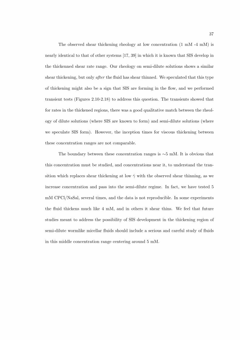
37

The observed shear thickening rheology at low concentration (1 mM -4 mM) is

nearly identical to that of other systems [17, 39] in which it is known that SIS develop in

the thickenned shear rate range. Our rheology on semi-dilute solutions shows a similar

shear thickening, but only after the fluid has shear thinned. We speculated that this type

of thickening might also be a sign that SIS are forming in the flow, and we performed

transient tests (Figures 2.10-2.18) to address this question. The transients showed that

for rates in the thickened regions, there was a good qualitative match between the rheol-

ogy of dilute solutions (where SIS are known to form) and semi-dilute solutions (where

we speculate SIS form). However, the inception times for viscous thickening between

these concentration ranges are not comparable.

The boundary between these concentration ranges is ∼5 mM. It is obvious that

this concentration must be studied, and concentrations near it, to understand the tran-

sition which replaces shear thickening at low γ with the observed shear thinning, as we

increase concentration and pass into the semi-dilute regime. In fact, we have tested 5

mM CPCl/NaSal, several times, and the data is not reproducible. In some experiments

the fluid thickens much like 4 mM, and in others it shear thins. We feel that future

studies meant to address the possibility of SIS development in the thickening region of

semi-dilute wormlike micellar fluids should include a serious and careful study of fluids

in this middle concentration range centering around 5 mM.

38

Chapter 3

Rising Bubble Oscillations:

A New Hydrodynamic Instability Observed

in Wormlike Micellar Fluids

3.1 Air bubbles rising through liquids

In chapter 2 we explored the rheology of certain wormlike micellar fluids. While

rheological tests provide quantitative information about the fluid (viscosity and relax-

ation time for example), these tests are very limited in that the flow is either pure

extension or pure shear. Rheology attempts to characterize the fluid by its material

paramaters, though it is well known that these properties depend in no small way on the

flow field. For viscoelastic fluids, rheology cannot be expected to lead to a prediction of

the fluid’s response to a general velocity field, since the stress is in general a non-linear

function of the rate of strain. In this chapter we look at a hydrodynamic experiment

that we performed with many wormlike micellar fluids. The experiment is to create an

air bubble at the bottom of a cylinder filled with micellar fluid, and then to examine

such properties as speed and shape of the bubble. This experiment is simple in that

it requires no extraordinary tools, and subjects a fluid initially at rest to the constant

average stress of the buoyancy of the bubble, which causes motion in the fluid.

While the motivation for such an experiment can be pure curiosity, the particular

choice of examining a rising air bubble is linked to previous experiments on rising bubbles

in other viscoelastic fluids, namely polymer solutions, as well as Newtonian fluids. In

39

either type of fluid, several different bubble shapes have been documented as well as

other interesting phenomena [75, 73, 22, 74]. And while bubbles in Newtonian fluids are

always smoothly curved (with the exception of turbulent flows), in polymer solutions

they can have a sharp cusp at their trailing end (Fig. 3.1). Furthermore, this cusp is

non-symmetric [22], that is, if the bubble is seen rotated 90, the sides would not meet

at a point [47]. The effect is a “knife edge”, and this edge itself does not always have

the same shape. An excellent account on the possible cusp shapes is given by Liu, Liao,

& Joseph [22].

Fig. 3.1. A rising cusped air bubble in a polymer solution (0.08% carboxymethylcellulosein 50:50 glycerol/water).

Another effect seen with rising bubbles in non-Newtonian fluids is the so called

“negative wake”, which refers to the direction of the fluid flow in the wake of the bubble.

40

In Newtonian fluids, the fluid follows the bubble in the wake, i.e. it flows up. In polymer

solutions it was first observed by Ole Hassager in 1979 [75] that the flow in the wake of

the bubble is down. A good analogy is with the wind created by a passing car; leaves

on the ground get whipped up behind the car, and then move in the same direction as

the car. Imagine instead the leaves going in the opposite direction and it becomes clear

that this negative wake is extremely counterintuitive and intitiates us to the world of

non-Newtonian fluids.

3.2 Bubbles in wormlike micellar fluids

On a microscale level, Newtonian fluids consist of molecules which can be ap-

proximated by point masses (such as air and water). Non-Newtonian fluids consist of

larger structures, such as polymer chains. This increased size affords a greater number

of degrees of freedom which leads to macroscopic viscoelasticity [47]. Wormlike micelles

are aggregates of amphiphilic molecules, long enough to resemble polymers [6], but with

the added feature that their length distribution is determined by aggregation kinetics

since micelles continually break and reform [2, 4, 16]. The molecular level physics is

more complicated for such fluids, and one can expect this will introduce a new set of

flow properties to the class of non-Newtonian fluids.

In particular, we can ask whether or not micellar fluids will be able to support

a sharp cusp on a rising bubble. The problem is that the stress in the fluid near the

surface of the bubble is proportional to the surface curvature (assuming a constant

surface tension) [47]. Evidently, fluids comprised of large (macro) molecules can support

the large stress at the cusp, but fluids of point particles (Newtonian fluids) do not. If the

41

stress in a micellar fluid is large enough to break the micelles, then they might not be

long enough to accomodate a cusp, resulting in Newtonian-like bubbles. It is interesting

to see the effect of stress and flow on the micellar kinetics, and we can ask the question:

will the impact on micellar kinetics be great enough to be seen macroscopically in the

rise of an air bubble?

Fig. 3.2. Cusp shape change of an oscillating bubble rising through a 15mM CPCl/NaSal(weight fraction ϕ = 0.5%) solution at T = 37.5C. The scale at left is marked incentimeters. Interval between pictures: 0.05 s.

The answer to this question is yes [19]. For certain wormlike micellar fluids, there

is in fact a sharp cusp at the trailing edge of a bubble, but it is unstable in the following

sense. In these wormlike micellar fluids we have observed the cusp extend to a sharp

point and then retract to a blunt edge, as shown in Figure 3.2. This effect repeats itself

during the entire rise of the bubble with no apparent sign of diminishing, as discussed and

shown below. More spectactular is what happens to the rise velocity during the cusp

42

shape change; the bubble velocity rapidly increases when the cusp retracts and then

slows again. Typically, bubbles begin to oscillate within 10 seconds of their formation,

with a similar time between oscillations.

These clearly visible velocity oscillations are apparently not a transient effect; we

have observed their persistence for rise distances larger than one meter, during which

there were more than 30 oscillations in ∼ 35 s (for 8 mM CPCl/NaSal), and velocities

more than doubled during a speed oscillation. Figure 3.3 tracks the position of a rising

bubble. Negative wakes were sometimes observed as well, but the observation was only

possible when a second bubble was in the wake of a higher bubble. In this case the

lower bubble would be pushed downward during the oscillation of the bubble above. It

is unclear whether a negative wake is present when the bubble is not oscillating, and we

could not determine this possibility.

In this chapter we present a detailed experimental survey of the oscillatory motion

of rising bubbles in a wormlike micellar fluid [76]. To study the role of the aggregation

kinetics of the micelles on the observed dynamics, both concentration and fluid tem-

perature were varied over a wide range. As these parameters change, different micellar

architectures are possible - from short linear or branched micelles to crosslinked net-

works [10, 26, 25]. Four types of bubble dynamics were seen: Newtonian behavior at

high temperatures, standard polymeric behavior, and two distinct oscillating responses

occurring in different concentration ranges. Steady rheology experiments were performed

to identify the fluid microstate, and we found that transitions in the equilibrium struc-

ture match transitions in bubble behavior. Critical temperature bounds were also found,

43

Fig. 3.3. Height z versus time t of an oscillating bubble in 8mM CPCl/NaSal at T=22.4C in a 1.2 m cylinder. The data shown is 40 cm high, and 11.4 seconds in duration.VMin = 2.5cm/s, VMax = 5.2cm/s, VAve = 3.4cm/s.

44

which can be interpreted as a minimum length of micelle required for oscillations to oc-

cur, so that for certain concentrations the fluid may be tuned with temperature to make

bubbles oscillate, rise with a stable cusp, or rise as bubbles in Newtonian fluids.

3.2.1 Preparation of fluids and experimental procedures

Non-transient oscillating bubbles were first observed in aqueous solutions of cetyltrimethy-

lammonium bromide (CTAB) and sodium salicylate (NaSal) [19]; here we use another fa-

miliar system, cetylpyridinium chloride (CPCl) and NaSal, with the fixed ratio [NaSal]/[CPCl]

= 1 [6]. The CPCl, NaSal, and NaCl were purchased from Sigma-Aldrich. The surfac-

tant and salts were dissolved in water which was deionized with a Barnstead B-Pure

purification system. Typical conductivity values for deionized water were in the range

16.5− 17.9 MΩ− cm. The procedure for making the fluids was:

1. The surfactant was combined with deionized water and mixed for one hour over a

low heat.

2 The NaSal was dissolved in deionized water and mixed by hand for five to ten

minutes.

3. After mixing the surfactant and water for one hour, the salts (dissolved in water)

were added to the surfactant solution. The heat was turned off and the solution

was allowed to mix for twenty four hours or more.

4. Before any use of the fluid for data collection, the mixed fluid was allowed to sit

undisturbed for three or more days.

45

All experimental results are for a single bubble rising near the center of the tube,

with volumes ranging from 14 mm3 to 110 mm3. The bubble was injected into the fluid

at the bottom of a plexiglas cylinder (31 cm height, 5 cm diameter) using a syringe with

a long stainless steel tube (inner diameter of either 1.0 mm or 1.5 mm). Great care was

taken to record data on a single bubble with the syringe, which was a difficult procedure

because often more than a single bubble was produced at a given time. Many trials

resulted in either multiple bubbles or a single bubble which was near the wall of the

cylinder. The plexiglas cylinder sat in a rectangular plexiglas tank (∼ 8 gallon capacity)

filled with tap water which was temperature controlled by a Neslab RTE-111 circulator

connected to the tank with two hoses. The water level in the tank was controlled with

adjustable clamps on the hoses, and was always at least five centimeters lower than the

top of the cylinder containing the wormlike micellar fluid.

Immediately following each bubble trial, the temperature of the micellar fluid was

measured by inserting a glass mercury thermometer (accurate to 0.1C) directly into the

micellar fluid. The temperature of the fluid was recorded only after it remained constant

for one minute or more. After the temperature was measured, the syringe was removed

and the cylinder was covered with parafilm. Both the syringe and thermometer were

washed by hand with mild soap and tap water, then rinsed first with ethanol (95% pure)

then deionized water and dried with Kimwipes. To allow the fluid to rest and return to

equilibrium, no less than one hour was allowed between succesive bubble trials on a given

fluid. When temperature was changed, no less than two hours was given for the fluid to

equilibrate after the fluid achieved the desired temperature. When a new concentration

was tested, the old fluid was discarded and the cylinder was washed with mild soap and

46

tap water, rinsed with deionized water and dried with compressed nitrogen. The new

fluid was poured into the clean cylinder, covered and allowed to equilibrate at room

temperature for no less than twenty four hours before any experiments were performed.

The ratio of the horizontal diameter of the bubble d to the cylinder diameter D

is d/D ≤ 0.14, and we have checked that bubbles oscillate for d/D ' 0.02. Typical

sizes for the Reynolds number (inertia) are Re ' 10−2−5, while the Deborah number

(elasticity) ranged from De ' 1− 500, similar to values seen for oscillating bubbles and

spheres in CTAB/NaSal [19, 20]. Rheological data were taken with a Rheometrics RFS-

III controlled rate of strain rheometer with circulating fluid temperature bath, using a

stainless steel Couette geometry. Video images were made with a Kodak Ektapro Motion

Analyzer (Model 1012), and a Vision Research, Inc. Phantom v5 CCD camera.

Birefringent images were made by placing the plexiglas cylinder between two

crossed polarizers, the Phantom CCD camera in front and a uniform light source behind.

Optical birefringence is a well-known technique for visualizing stress in non-Newtonian

fluids [34], and is especially effective for wormlike micellar fluids [35]. Before reaching

the micellar fluid in the cylinder, the light is linearly polarized, and then blocked on

its way to the camera by the second polarizer. In this arrangement, when the fluid is

at rest (and is isotropic), no light reaches the camera. The anisotropy (alignment of

micelles) of the fluid caused by the rising bubble rotates the polarization of the light in

the fluid and allows only some light to reach the camera. Birefringence occurs when the

polarizers are either parallel or perpendicular to the alignment of the micelles in order to

obtain birefringence. The result is light regions in the fluid representing different local

47

alignments of micelles, which means the micelles are stretched from their equilibrium

coiled configurations. We therefore associate stress with the light regions in the fluid.

3.2.2 Concentration and temperature dependence

We have studied concentrations from 4 to 40 mM (weight fractions 0.13% ≤ ϕ ≤

1.3%). From 5 to 15 mM, bubbles have a cusp which oscillates in length and changes

shape (Fig. 3.2). While rising, the cusp lengthens (frames 1-4 in Fig.3.2) during which

the velocity as measured at the top of the bubble is nearly constant. At the apex of

the extension, the tail abruptly retracts and the bubble jumps upward (frames 4 and

5). After this it slows to a nearly constant velocity until the cycle repeats. We call this

behavior type I oscillations, which occurs in the temperature ranges shown in Fig.3.4

and is consistent with the oscillations previously observed in CTAB/NaSal [19].

Above a critical temperature in the type I range (Fig.3.4), bubbles have a sharp

cusp which does not change in length (“steady cusp” in Fig.3.4) and velocities smoothly

reach a steady state as in polymer solutions, i.e, the oscillatory instability vanishes. By

60C, the solutions appear Newtonian (“no cusp” in Fig.3.4): large enough bubbles are

ellipsoidal and undergo the well-known side-to-side oscillations [27]. In this temperature

range, the micelles must be predominantly spherical or more like rigid rods [2] neither

of which are not stretched by the passing bubble.

Upon increasing the concentration from 15 mM to 16 mM (ϕ = 0.5% to 0.53%),

all oscillations cease. Bubbles rise steadily with a stable cusp, for concentrations up

to 20 mM in temperature ranges shown in Fig.3.4, but there are no temperatures at

which oscillations occur. This is puzzling, as these fluids are still viscoelastic, consist

48

20 25 30 35 40 45 50 55 60

4

6

810

30

no cuspsteady cusposcillations

Temperature [°C]

Con

cent

ratio

n [

mM

]

I

II

Fig. 3.4. Temperature and concentration phase diagram for the dynamics of a risingbubbles in equimolar CPCl/NaSal, showing two distinct regions of oscillating behavior(shaded) labelled as I and II. The straight line at low concentrations is an isoline ofequation 3.1 and marks a boundary for type I oscillations.

49

of wormlike micelles, and have a rheology similar to type I fluids (discussed below).

Note that the transition temperature from polymeric to Newtonian behavior reaches a

maximum at this concentration (Fig.3.4).

More surprising is the re-emergence of oscillations for concentrations from 25 mM

to 40 mM (0.8% ≤ ϕ ≤ 1.3%). Yet here the oscillations, which we call type II, are

visibly different from those at lower concentrations (Fig. 3.5); the shape change involves

the entire bubble, whereas in type I it seems restricted to the tail and cusp. A type

II oscillation begins with a constriction in width near the top of the bubble, while the

whole bubble lengthens. This constriction then travels downward, as if the bubble were

squeezing through a hoop. We define wmax to be the maximum (relaxed) width (at

its waist), wmin to be its most constricted width, and ∆w = wmax − wmin, we found

∆w/wmax ' 0.13 in type II fluids and 0.04 in type I. Length extensions, however, were

∆l/lmin ' 0.25 in type II and 0.27 in type I; for previously observed bubbles rising

in CTAB/NaSal, ∆l/lmin ' 0.26 [19]. This previous study revealed only one type of

oscillation, which due to the shape dynamics we identify as type I [19].

Although wormlike micelles are comprised of surfactants, it is unlikely that surface

tension plays a role in the mechanism of bubble oscillations; falling rigid spheres have also

been observed to oscillate in wormlike micellar fluids [20, 36]. Figure 1 in the article by

Jayaraman and Belmonte [20] is an overlaid time series of a solid sphere in a wormlike

micellar fluid made from 9mM CTAB/NaSal. The time interval between images is

constant, though the spacing between succesive sphere positions is not, and indicating

speed oscillations. Furthermore, our observation of two types of oscillation suggests that

the viscoelastic character of the bulk fluid is changing with concentration. We address

50

Fig. 3.5. Oscillating bubble in 30mM CPCl/NaSal at T = 21C. Interval betweenpictures : 0.24 s.

this with rheology measurements, controlling the shear strain rate γ and recording the

effective viscosity, ηeff = σxy/γ, where σxy is the steady shear stress. Transient tests

were also performed, to ensure that steady state was achieved (see chapter 2). Shown in

Fig.3.6a is ηeff as a function of γ at 30C, for concentrations in both oscillation regions,

as well as the non-oscillating range between them. All fluids are shear thinning: ηeff

decreases at high enough γ. While there is a noticable difference in the rheology upon

increasing from 20 to 30 mM, 30 and 40 mM (type II region) are strikingly similar;

they have a constant viscosity over a broader range of γ than the other fluids. More

interestingly, the zero shear viscosity, η0 (defined as the plateau value at low γ [47]),

decreases with concentration. As concentration increased, there is more material to form

micelles and we would expect them to thus be longer, which would increase viscosity.

The observed decrease is therefore another counterintuitive aspect of wormlike micellar

fluids.

51

0.001

0.01

0.1

1

1 0

1 0 0

1 1 0

η 0 (

Poi

se)

Concentration (mM)

I II

0.1

1

1 0

1 0 0

0.01 0.1 1 1 0 1 0 0

10 mM20 mM30 mM40 mM

Shear Rate (s- 1

)

η eff (

Poi

se)

a )

b )

Fig. 3.6. Rheology of equimolar CPCl/NaSal at T = 30C: a) effective viscosity versusshear rate for 10, 20, 30, and 40 mM CPCl/NaSal; b) zero shear viscosity, η0 as afunction of concentration. The shaded regions mark the concentration ranges of bubbleoscillations.

52

3.2.3 Inferred length dependence

The changes in temperature and concentration introduce variations in the fluid

microstructure, among which is the micellar length. For low concentrations in equilib-

rium, the average length of a wormlike micelle L0, can be described within a mean field

approximation [9, 2, 5]:

L0(φ, T ) ∼√

φ eE/2kT (3.1)

where φ is the total amphiphile concentration, k is Boltzmann’s constant, T is tem-

perature, and E is the scission energy required to break one wormlike micelle into two

wormlike micelles. The scission energy is directly related to the energy required to sus-

tain an endcap of a micelle. To break a micelle in two requires the formation of two new

endcaps, so the scission energy is exactly twice the endcap energy. Estimates based on

light scattering measurements for E are on the order of 10kT [9, 37, 25] - much lower

than the covalent bonds of polymers, yet large enough for some micelles to reach appre-

ciable lengths against thermal fluctuations [9]. The flow near the bubble may increase

the equilibrium length, and there is evidence that shear-induced structures (SIS) much

larger than individual micelles form in such flow in both CTAB/NaSal [17, 38, 39] and

CPCl/NaSal [40, 41]. We assume simply that for the type I region, L0 is the relevant

quantity determining whether or not the bubble oscillates. Specifically, we attribute the

oscillations to a breaking instability of micelles or SIS in the bubble wake, occurring only

if L0 exceeds some critical value Lc. Using equation.3.1, the solid line in Figure 3.4 is

an isoline of L0 corresponding to a scission energy of E = 1.01× 10−19 Joules, which is

about 24kT .

53

Type II oscillations have a much simpler dependence on temperature; they occur

only for T . 36C (Figure 3.4). If crosslinks have indeed formed, then the mean field

length is no longer an appropriate quantity. The transition temperature Tc = 36C

suggests a critical energy condition (Ec ' 4.3 × 10−21 Joules), much smaller than the

endcap (scission) energy, which may describe the transition from junctions to endcaps.

Thus for T > Tc, endcaps would dominate and the fluid is comprised of individual

micelles which can entangle like polymers. For T < Tc, the microscale structure remains

a crosslinked network of micelles fused at junction nodes. Though this is at present only

speculation, it is consistent with both the rheology and the rising bubble dynamics.

3.2.4 Topological phase transition

The overall dependence of η0 on ϕ is complicated, and indicates transitions in

micellar microstructure. This is shown in Fig.3.6b, in which the different oscillation

regimes are shaded. The transition at low concentration from constant η0 to rapid

growth marks the overlap concentration ϕ∗ ' 3 mM, below which the viscosity is similar

to the viscosity of the solvent, and this is therefore called the dilute regime. Above ϕ∗

the fluid viscosities begin rapid growth. The region above ϕ∗ is clearly distinguished

from the dilute, and we call this the semi-dilute regime. In the semi-dilute regime it is

reasonable to assume that micelles exist as individual worms in a disordered entangled

network [42], which would account for the higher viscosities. Here we find η0 ∼ ϕ5.5,

close to the value 5.4 associated with the relaxation of stress by reptation [10, 29]. The

semi-dilute regime ends near ϕ ' 12 − 15 mM, and is followed by an extraordinary

54

decrease of η0 with concentration, which continues to approximately ϕ ' 30 mM, after

which η0 varies weakly.

The dramatic change in the concentration dependence of η0 indicates a transition

in the equilibrium fluid structure, coinciding with the loss of type I oscillations. It may be

that the entangled micelles in the semi-dilute range have begun to fuse at entanglement

points, forming a crosslinked network [10, 29, 31, 32]. The crosslinked network state of

micellar structure was also proposed for another wormlike micellar system which shares

rheological properties with our type II fluids [10], among which are the broad zero shear

viscosity plateaus. The junction nodes are free to slide along the micelles in such a

formation, which would account for the decrease in viscosity. We assume that the ratio

of crosslinks to entanglement points would grow as η0 decreases, until the new state is

fully formed and η0 stabilizes near ∼ 30 mM = 1%. A crosslinked network state was

also proposed by Lequeux and Candau [33] for systems of CTAB/NaSal at ϕ ' 1%, and

it is noteworthy that CTAB/NaSal solutions also give rise to oscillating bubbles [19].

Transitions in micellar morphology would naturally lead to transitions in the

mechanisms for stress relaxation, which should be observable in the stress field around

the rising bubble. These transitions are made evident through birefringent visualization,

shown in Fig.3.7 for the three concentration regimes, in which bright areas correspond

to anisotropic fluid (see Chapter 2 section 1). Fig.3.7a (10 mM) shows the localization of

stress in the wake of a type I oscillating bubble. This birefringent tail mirrors the dynam-

ics of the bubble’s cusp (Fig.3.2), and when the cusp retracts upward, the birefringent

tail disperses to the sides. At 20 mM a similar - but shorter - tail is seen (Fig.3.7b), whose

length remains constant, like the bubble tail. Fig.3.7c corresponds to type II oscillations

55

Fig. 3.7. Birefringent images of the wake behind a bubble rising in CPCl/NaSal atT = 24C: a) 10 mM ; b) 20 mM ; c) 35 mM. Each image is 6.5 cm high. The diametersof the bubbles are all in the range of 3 mm to 5 mm. Reynolds and Deborah numbers foreach image are: a) Re ' 4.72, De ' 250; b) Re ' 0.02, De ' 6; c) Re ' 1.1, De ' 1.8.

56

(35 mM), in which three equally spaced birefringent bands or wings indicate a broader

distribution of stress. This pattern is slightly altered during the course of an oscillation:

the lateral birefringent wings move down a little the bubble during an oscillation and

rise again afterwards. These images clearly show that each type of oscillatory motion is

matched by a unique stress response in the fluid.

3.2.5 Other types of wormlike micellar fluids

The different oscillations we have observed appear linked to two different mi-

croscale architectures as we have shown. We extended our study to include the well

characterized ternary system CPCl-NaSal diluted in concentrated NaCl, with a ratio

[NaSal]/[CPCl] = 0.5 [42, 43, 16]. We tested several concentrations of these fluids for

oscillating bubbles in our apparatus (Table 3.1) at T = 30C, a temperature central to

both type I and II oscillations (Fig.3.4).

Experiment [CPCl] [NaSal] [NaCl]

1 30mM 15mM 500mM

2 40mM 20mM 500mM

3 50mM 25mM 500mM

4 60mM 30mM 500mM

5 70mM 35mM 500mM

6 80mM 40mM 500mM

Table 3.1. Alternate wormlike micellar systems tested which produced no oscillatingbubbles.

57

A typical bubble shape is shown in Figure 3.8. We observed no oscillations or

any behavior different from steadily rising bubbles in conventional polymeric fluids [22].

This ternary system is known to consist of entangled wormlike micelles, which when

taken with the observed scaling η0 ∼ ϕ3.3 [30], indicates that micellar breaking is the

dominant stress relaxation mechanism (occurring on a shorter timescale than reptation)

[9, 42]. The observed scaling law for η0 for our fluids in the semi-dilute regime indicates

stress relaxation by reptation rather than micellar scission kinetics. This difference could

account for the absence of oscillations in the ternary system with added NaCl. If so, the

type I oscillatory motion of rising bubbles would not be a characteristic of fluids in this

“fast-breaking” limit [9, 30].

We may still ask why this ternary system could not support type II oscillations,

and a clue is offered through our conjecture of a crosslinked network. The ternary

systems we tested that failed to produce oscillating bubbles (given in Table 3.1) have

been well studied and no decrease in zero shear viscosity has been reported as surfactant

concentration was increased [42]. Using similar techniques, it was found that in other

wormlike micellar systems the size of micelle decreased as concentration was increased

[44, 45] and it was again proposed that these systems were in a crosslinked network state.

The data collected by Berret et al. [42] for the ternary sytem we have tested led experts

in the field to conclude that these ternary systems “are prototypes for entangled but

not branched wormlike micellar systems” [42]. Perhaps then the crosslinks (branches)

are essential in producing type II oscillations. There is at present not enough data on

bubble oscillations to put this conjecture on firm ground, though all of the evidence

58

collected so far (here and elsewhere) on wormlike micellar fluids either supports it or

fails to contradict it.

Fig. 3.8. Rising air bubble in 80 mM CPCl - 40 mM NaSal diluted in 500 mM NaCl.The cusp is stable and no oscillations were observed.

Wormlike micelles are far more delicate structures than polymers as constituents

of complex fluids, and the interplay of their microscopic dynamics with macroscopic flow

promises to include novel instabilities to the class of viscoelastic fluids. Indeed, the os-

cillatory motion of a rising bubble through a wormlike micellar fluid illustrates some of

the dramatic possibilities of this coupling. Lengths of micelles can change locally with

flow, and micelles may themselves aggregate into SIS. We have shown that this response

to flow can in fact be tuned by the choice of temperature and concentration, and the

effects can produce dynamics in which the forces never balance - no steady state is ob-

served, despite viscous damping. Beyond bubble dynamics, this ‘tunable fluid’ provides

a wide variety of different dynamics (Newtonian, polymeric, time-dependent) which may

59

be useful as either a biomolecular medium or as a versatile industrial fluid. The dynamic

behavior of a rising bubbles demonstrates the possible variety of hydrodynamic effects

and their sensitivity to physical microstructure in wormlike micellar fluids.

60

Chapter 4

A New Constitutive Model

for Wormlike Micellar Fluids

4.1 Basics of rheology

As was seen in Chapters 1 and 2, non-Newtonian fluids have very different flow

properties from viscous Newtonian fluids. Chapter 1 gave examples of the elastic nature

of polymer liquids as well as mathematical descriptions of both types of fluids, and Chap-

ter 2 introduced wormlike micellar fluids and examined ways they differ from Newtonian

and other non-Newtonian fluids through experimental rheology. Chapter 3 examined an

interesting instability, and differentiated wormlike micellar fluids from classical polymer

solutions. With this as background, we have enough information about these fluids to

begin to consider them from a mathematical perspective. In this chapter we consider

what physical aspects of wormlike micellar fluids can account for their unusual flow prop-

erties, and how we can begin to model them. To this end, we briefly review concepts

from previous chapters which will be relevant to modelling.

For Newtonian fluids, we know that σ = 2ηD, in which η is a constant known as

the viscosity and D is the symmetric part of the velocity gradient: D = 12(∇u +∇uT ).

61

If the flow is pure shear, then in Cartesian coordinates

D =12

0 γ 0

γ 0 0

0 0 0

,

where γ is known as the shear rate. In the case of steady shear flow, γ is a constant, and

we can view the shear component of stress σxy as a function of γ. Note that σxy = σyx

are the only non-zero components of stress in pure shear flow; in extensional flows the

diagonal components of D would not be zero. For any Newtonian fluid, the steady

state value of σxy grows linearly with γ, and the slope is simply the viscosity η. For

viscoelastic fluids, typically there is a range of small values of γ for which σxy depends

linearly on γ [3]. This is because in equilibrium the macromolecule (or micelle) will be

“coiled” up, and for small enough shear gradients, it will not unravel, but move through

the fluid like a colloidal sphere. The internal degrees of freedom not being activated, the

macromolecules behave like large point particles, and the fluid seems Newtonian. In this

“Newtonian” region the linear proportionality constant is called the zero shear viscosity

and denoted by η0.

At higher shear rates, deviations are often experimentally observed [3]: if σxy

grows slower than η0γ, we say the fluid is shear thinning, and if σxy grows faster than

η0γ, it is shear thickening. Since for non-Newtonian fluids, σxy is often no longer linearly

proportional to γ, it is inappropriate to speak of a single viscosity, and the effective

62

viscosity is defined as ηe = σ/γ in analogy to Newtonian fluids [47]. Thus at low shear

rates, ηe = η0, and at higher γ we would have ηe < η0 for shear thinning fluids.

In general, any constitutive equation used to model a fluid should capture, at least

qualitatively, those material parameters which play a role in the effects under study;

if elasticity is important for example, then the constitutive equation should predict a

relaxation time. Unlike Newtonian fluids, there is no single constitutive equation which

succesfully describes all viscoelastic fluids, even for a given type of flow [77]. Instead,

various models are used depending on particular circumstances of the fluid, the flow and

the phenomena under investigation. A first approach to modelling viscoelasticity came

from J.C. Maxwell in 1867 [48]:

σ + λ∂tσ = 2η0D. (4.1)

The Maxwell equation introduces a new material parameter in λ, which is a time con-

stant, while η0 is the zero shear viscosity (a constant). The λ ∂tσ term is the elastic

contribution, the other terms give the Newtonian constitutive relation if λ = 0. The

meaning of λ becomes more clear when we solve this first order linear ordinary differen-

tial equation using the integrating factor et/λ:

σ =2η0λ

∫ t

0e(t′−t)/λD(t′)dt′. (4.2)

In this form it is easy to see that elasticity has been accounted for in the form of memory.

That is to say, stress is determined not only by what the current velocity gradient is,

63

but the velocity gradient at all previous times. The decaying exponential term can be

thought of as a weight, so that D(t′) contributes less the farther back in time one goes,

and λ is a measure of the amount “forgotten” about D as we look back in time. This

model is sometimes referred to as having “fading memory” for this reason [47].

The Maxwell model (equation 4.1) gives a plausible description of elasticity, but

some underlying physics is not entirely correct. The problem is that when we consider

an equation for fluid motion, we must remember that we are describing an object (a fluid

“packet”) which is moving. If we use spatial variables (x1, x2, x3) and a time variable

t then, since the position of a fluid particle is moving, xi = xi(t). It is well known [78]

that it is not physically correct to use a partial time derivative in the Maxwell equation,

but rather the total time derivative of σ should be used:

d

dtσ(x(t), t) =

∑

i

∂σ

∂xi

∂xi∂t

+∂σ

∂t

=∑

i

ui∂σ

∂xi+

∂σ

∂t

= u · ∇σ +∂σ

∂t(u is the velocity)

The total time derivative (sometimes denoted with capital letters DDt = u · ∇ + ∂

∂t) is

called the convective or material derivative. The alteration to 4.1 using this derivative

is commonly called the convected Maxwell model:

σ + λ (u · ∇σ +∂σ

∂t) = 2η0 D.

64

The convected Maxwell model differs from equation 4.1 in the nonlinear term

u ·∇σ. For the remainder of this thesis we assume our flow to be homogenous, for which

u · ∇σ = 0, so that the two forms of the Maxwell model are identical.

Although the Maxwell model includes a term to account for relaxation, in steady

shear flow it predicts σxy = η0γ, so that ηe is constant equal to the zero shear viscosity,

and no thinning or thickening is possible. One can easily write models which allow for

the nonlinear viscoelasticity, for instance a power law model such as σ = η0γk, gives

ηe = σγ = η0γk−1, which is no longer constant with γ as long as k 6= 1. The White-

Metzner model [47] incorporates nonlinear viscoelasticity directly in the Maxwell model:

σ +η(γ)G

∂tσ = 2 η(γ) γ.

In this model η(γ) can be any function such as a power law, or it can be determined by

fitting to data. Note that here we restrict ourselves to pure shear flow.

In our endeavor to model wormlike micellar fluids, we choose to start with the

Maxwell model for its elegant way of including elasticity through memory and describing

fading memory with a decaying exponential kernel. Our alterations to the Maxwell model

will be motivated by the idea of memory in wormlike micellar fluids and the particular

microscale physics these fluids posess.

4.2 Review of existing models for wormlike micellar fluids.

Wormlike micellar fluids began receiving increased attention in the early 1980’s

after several experimental results were published showing that these fluids have unusual

65

and often unprecedented responses to flow [49, 6]. The experimental and theoretical

challenge was to understand what had been been observed as well as predict how the

fluids would react to flow. The general problem facing the theoretician is to understand

what are the prominent properties a system posesses, and which are relevant or respon-

sible for specific observations. This is only the first step though, since there can be

many such properties and they in general depend on each other. So there is the prob-

lem of understanding the physical processes, followed by or simultaneously developed

with a mathematical description, of which there may be many. This is the problem of

modelling. In this section we provide a brief overview of previous models put forth to

describe wormlike micellar fluids.

In developing a theory, a standard mindset is to compare the given problem to

an analogous problem. In the case of wormlike micelles, which may be long and flexible,

there is an obvious comparison with polymers. A polymer solution is in some sense the

standard when describing macromolecular or non-Newtonian fluids, though there are

many non-Newtonian fluids which consist of particles very different from polymers (e.g.

dense colloidal suspensions, clays, corn starch). Many constitutive equations have been

written to describe the fluid properties of polymer solutions [47, 77, 3], and this offers

a starting point in modelling wormlike micellar fluids. The next step is to identify key

differences from the analogous system and then adapt the equations to include these new

effects. When we compare wormlike micelles to polymers, one salient difference is the

reversible scission reactions of the micelles. So the idea would be to model this aspect

and incorporate it into a pre-existing constitutive equation. This is a common technique

in modelling wormlike micellar fluids [50, 51, 52, 53].

66

The ability of wormlike micelles to break and also combine affects the fluid in

many ways, and one example is the distribution of micelle lengths. While classical

polymer solutions may be polydisperse (i.e. there are polymers of varying lengths in a

given fluid), once the polymers are formed, the size distribution is fixed. In the case

of wormlike micelles, the size distribution is in thermal equilibrium (more precisely,

chemical equilibrium), since breaking and recombining events persist when the fluid

is not moving [9, 2]; recall chapter 3 in which a mean field model prediction for the

average length of micelles and the length distribution in equilibrium. It is very sensible

to imagine that flow will increase the average number of collisions between micelles and

it becomes obvious to ask how this will affect the length distribution. This question has

received a good deal of attention in the fluids community because of some astounding

rheological effects, such as shear banded flow and shear thickening [17, 11, 54, 39] in which

the micelles aggregate to form larger structures, sometimes referred to as “bundling”,

forming a shear induced phase (SIP) or shear induced structure (SIS). Modelling this

“gelation” has provided some insight into the mechanism at work, but the reasons why

it occurs is still not understood.

While we review papers in this section to give the reader an idea of what has been

done in modelling micellar fluids or related subjects, there are many other articles which

have had an impact on the theory of these fluids. We list some of these models here and

give a brief description of their approach:

67

1. M. E. Cates (1987) [50] and M. E. Cates (1990) [51] - an adaptation of deGennes’

reptation model is presented (known as the “reaction-reptation model), which in-

cludes the effects of reversible scission reactions.

2. N. A. Spenley, M. E. Cates, & T. C. B. McLeish (1993) [81] - a simulation of

the reaction-reptation model [50] to predict the nonlinear rheology of wormlike

micelles, including a stress plateau associated with shear banding.

3. V. Schmitt, C. M. Marques, & F. Lequeux (1995) [55] - a constitutive equation is

presented which includes effects of flow on concentration, creating spatial concen-

tration gradients to describe shear induced phase separations.

4. B. H. A. A. van den Brule & P. J. Hoogerbrugge (1995) [56] - a simulation of rheo-

logical properties, including Brownian motion of a crosslinked network of molecules

which can detach and reattach themselves.

5. I. Jeon (1997) [57] - solutions to coagulation-fragmentation equations are approxi-

mated by Markov chains, and their qualitative behavior is studied.

6. A. Vaccaro & G. Marrucci (2000) [58] - a model describing a network (or “web”) of

polymers which may detach themselves and reattach elsewhere, much like micelles.

7. J. L. Goveas & P. D. Olmsted (2001) [59] - micelles are treated as chemical reactants

and a reaction-diffusion equation is written to model to study phase separation due

to flow.

In addition, we now review four other important papers in more detail.

68

8. R. Bruinsma, W. Gelbart, & A. Ben-Shaul (1992) [60]. This model describes

the effect of flow on the micellar length distribution with a “coagulation-fragmentation”

model to count the number of micelles of a given length. Bruinsma et al. use theory first

developed by Paine [61] in 1912 and von Smoluchowski [62] in 1916, for the coagulation

seen in colloidal suspensions under shear flow. Colloidal spheres were experimentally

seen to aggregate in shear flow [61] due to hydrodynamic interactions. This is called

orthokinetic coagulation, in contrast to perikinetic coagulation which occurs under the

influence of Brownian motion. The authors argue that we may expect orthokinetic

coagulation to begin to dominate over perikinetic at a critical shear rate γc = Dt/R2,

where Dt is the translational diffusion coefficient, and R is the radius of the sphere. The

derivation of this value for γc comes from the comparison of particle fluxes due to flow

and Brownian motion. Assuming the reaction cross section for coagulation is just the

particle radius, the flux due to shear is Js ∝ v A, where v is the impact velocity and A is

the reaction cross section. Assuming A = R2 and v = γ R, gives Js = ϕ(R)γR3 where

ϕ(R) is the concentration of particles with radius R. A similar argument for the flux

due to Brownian motion gives the relation Jb ∼ DtϕR R. The ratio of these quantities

gives the Peclet number for the flow: Pe = Js/Jb = γR2/Dt. When Pe > 1 orthokinetic

coagulation dominates, and γc is defined for Pe = 1. When applied to wormlike micelles,

R is replaced with the length L, so that the shear rate at which “gelation” or thickening

occurs grows like γc ∝ 1/L2. This is a nice result because it follows from very simple

and seemingly reasonable ideas, and the prediction makes sense: for longer micelles,

gelling will occur at more modest rates, that is, it is easier to induce coagulation since

the micelles are so long to begin with.

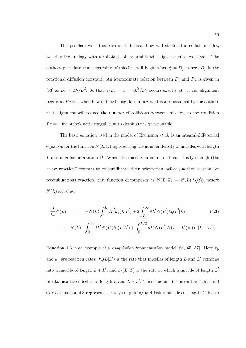
69

The problem with this idea is that shear flow will stretch the coiled micelles,

weaking the analogy with a colloidal sphere, and it will align the micelles as well. The

authors postulate that stretching of micelles will begin when γ = Dr, where Dr is the

rotational diffusion constant. An approximate relation between Dt and Dr is given in

[63] as Dr ∼ Dt/L2. So that γ/Dr = 1 = γL2/Dt occurs exactly at γc, i.e. alignment

begins at Pe = 1 when flow induced coagulation begin. It is also assumed by the authors

that alignment will reduce the number of collisions between micelles, so the condition

Pe = 1 for orthokinetic coagulation to dominate is questionable.

The basic equation used in the model of Bruinsma et al. is an integral-differential

equation for the function N(L, Ω) representing the number density of micelles with length

L and angular orientation Ω. When the micelles combine or break slowly enough (the

“slow reaction” regime) to re-equilibrate their orientation before another scission (or

recombination) reaction, this function decomposes as N(L, Ω) = N(L) fL(Ω), where

N(L) satisfies:

∂

∂tN(L) = −N(L)

∫ L

0dL′kb(L|L′) + 2

∫ ∞L

dL′N(L′)kb(L′|L) (4.3)

− N(L)∫ ∞0

dL′N(L′)kc(L|L′) +∫ L/2

0dL′N(L′)N(L− L′)kc(L

′|L− L′).

Equation 4.3 is an example of a coagulation-fragmentation model [64, 65, 57]. Here kb

and kc are reaction rates: kc(L|L′) is the rate that micelles of length L and L′ combine

into a micelle of length L + L′, and kb(L′|L) is the rate at which a micelle of length L′

breaks into two micelles of length L and L− L′. Thus the four terms on the right hand

side of equation 4.3 represent the ways of gaining and losing micelles of length L due to

70

coagulation (combining) and fragmentation (breaking). When collisions occur quickly,

the authors argue that the many collisions randomize the orientation of micelles before

coagulation or fragmentation, so that equation 4.3 again holds in this ”fast reaction”

regime.

In thermal equilibrium, the reversible scission reactions of micelles are expected

to obey the law of detailed balance, which says that for each breaking event there is a

recombining event, which gives a steady state length distribution N(L). Detailed balance

requires that

N(L′) N(L− L′) kc(L′|L− L′) = N(L) kb(L|L′) + N(L) kb(L|L− L′). (4.4)

The breaking rates on the right hand side of equation 4.4 must be equal by symmetry

of the breaking event: a micelle of length L which breaks to give a micelle of length L′

necessarily makes a micelle of length L−L′ as well, so that kb(L|L′) = kb(L|L−L′). This

does not mean however, that these breaking reactions are identical; they are considered

distinct events because they involve different angular orientations. The authors solve

equation 4.4 in the case where L = 2L′ to obtain solutions of the form:

N(L) ∝ 1

g(L)1/ln 2e−L/L, (4.5)

in which L represents the average length. An exact solution to equation 4.3 is found

in equilibrium which has the form of the detailed balance solution (equation 4.5) with

g(L) = constant, with an average length L depending on concentration, temperature,

71

and scission energy in precisely the same way predicted by the mean field equilibrium

length model presented in chapter 2, i.e. L0 ∝ ϕ1/2eE/2kT . Hence equilibrium requires

that g(L) be constant in equation 4.5.

Although equations 4.4 and 4.5 hold only in equilibrium, and may not hold for

γ 6= 0, the authors assume that length distributions N(L) with flow are still of the form

of equation 4.5. For this model, the effect of flow is restricted to the ratio of rates g(L),

i.e. g(L) is allowed to be non-constant and L is solved for self-consistently. This is a

perfect example of the techniques of modelling we described at the beginning of this

section. So far, certain assumptions have been made, but they have all been reasonable

and physically motivated, and only solutions in equilibrium have been discussed, for

which there are existing models. The coagulation-fragmentation model given in equation

4.3 seeks to extend those results, and it has been shown to at least recover the accepted

equilibrium results. Now we come to the heart of the matter, namely, how does flow affect

the equilibrium distribution? By assuming that non-equilibrium solutions to equation

4.3 have the same general form as the equilibrium solutions, except that g(L) is flow

dependent, the authors have chosen to model the influence of flow in a specific way: the

effects of flow enter the equations only through the reaction rates kb and kc.

The remaining task is then to describe the ratio g(L). Starting from the analogy

to colloidal spheres, different forms for g(L) are assumed, depending on flow rate and

collision rate. Parameter space is partitioned into four cases: Peclet number Pe À 1,

or Pe ¿ 1, and the “slow reaction” versus the “fast reaction” regime. Bruinsma et al.

obtain the distribution N(L) in analytic form for these cases, which are used to obtain

72

expressions describing L. Using the relation

dL

dt= α(L)

∫ ∞0

∂N(L)∂t

dL (4.6)

in which α(L) is a different function of L for the cases Pe À 1 and Pe ¿ 1, together

with the coagulation-fragmentation equation (4.3), an ordinary differential equation is

obtained for L in each of the four cases. Rather than attempting to solve for analytic

forms for L, its steady state value can be obtained by minimizing the function v(L)

defined by

− d v(L)dL

≡ dL

dt.

It is natural to think of v(L) as a sort of potential for L. The results for the four cases

are [60]:

i) Pe ¿ 1, slow reaction regime:−L is shifted to only a slightly larger value than

L0, specifically, L ' L0(1 + Pe). We must remember that Pe ∼ γ and assuming

R2/Dt is O(1), we may conclude that γ is small in this formula.

ii) Pe À 1, slow reaction regime: L ∼ L0 Pe1/3, so that while Pe is much greater

than in case i), L grows even more slowly in this regime. Physically, we can say

that the stronger flow increases alignment and decreases reaction cross sections.

iii) Pe ¿ 1, fast reaction regime: In this case the “potential” v(L) has a local minimum

near L0 followed by a local maximum, i.e. there is a potential “well” and “barrier”.

This means that if the flow is strong enough (still with Pe ¿ 1) or the reaction

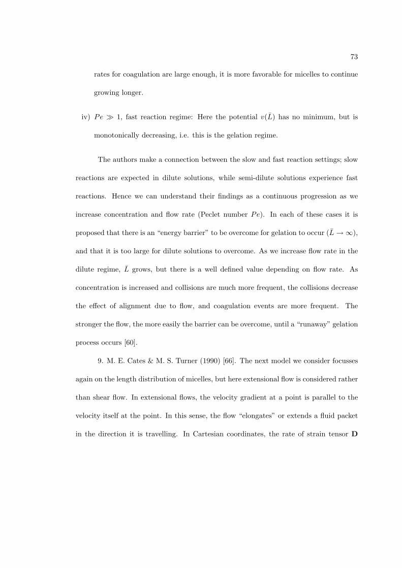
73

rates for coagulation are large enough, it is more favorable for micelles to continue

growing longer.

iv) Pe À 1, fast reaction regime: Here the potential v(L) has no minimum, but is

monotonically decreasing, i.e. this is the gelation regime.

The authors make a connection between the slow and fast reaction settings; slow

reactions are expected in dilute solutions, while semi-dilute solutions experience fast

reactions. Hence we can understand their findings as a continuous progression as we

increase concentration and flow rate (Peclet number Pe). In each of these cases it is

proposed that there is an “energy barrier” to be overcome for gelation to occur (L →∞),

and that it is too large for dilute solutions to overcome. As we increase flow rate in the

dilute regime, L grows, but there is a well defined value depending on flow rate. As

concentration is increased and collisions are much more frequent, the collisions decrease

the effect of alignment due to flow, and coagulation events are more frequent. The

stronger the flow, the more easily the barrier can be overcome, until a “runaway” gelation

process occurs [60].

9. M. E. Cates & M. S. Turner (1990) [66]. The next model we consider focusses

again on the length distribution of micelles, but here extensional flow is considered rather

than shear flow. In extensional flows, the velocity gradient at a point is parallel to the

velocity itself at the point. In this sense, the flow “elongates” or extends a fluid packet

in the direction it is travelling. In Cartesian coordinates, the rate of strain tensor D

74

would be diagonal, for example in elongational extension we have [47]:

D =

− ε2 0 0

0 − ε2 0

0 0 ε

(4.7)

In this matrix form for D, the extensional rate ε has units of inverse seconds and may be

constant or time dependent, and for inhomogenous flows may also be spatially dependent.

It is completely analogous to the shear rate γ in shear flows. Notice that extensional

flows have no shear component to them, and are examples of shear-free flows.

Because micelles are thought to be highly aligned in such flows, the model given

by Cates and Turner [66] assumes that micellar reactions (combining and breaking)

involve only collinear micelles. These authors also seek a mechanism for gelation to

occur, and the rough idea is that alignment will increase collisions and reactions because

all collisions here are for collinear micelles, making micelles longer. The longer micelles

will then have less angular mobility and will therefore be more easily aligned, which in

turn enhances growth again, and a gelation is predicted at a critical flow rate ε.

In this paper, the concentration of rod like micelles with length L and angular

orientation u is denoted by ψ(L,u), which is implicitly time dependent. The goal is to

find steady state solutions, i.e. solutions dψdt (L,u) = 0. Turner and Cates decompose dψ

dt

into the sum of two contributions: dψdt = F1 + F2, with F1(ψ) describing rotations and

angular diffusion, and F2(ψ) accounting for micellar scission and recombination. While

the functional form for F2(ψ) is a coagulation-fragmentation equation very similar to

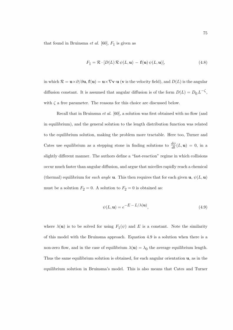
75

that found in Bruinsma et al. [60], F1 is given as

F1 = R · [D(L)Rψ(L,u) − f(u) ψ(L,u)], (4.8)

in whichR = u×∂/∂u, f(u) = u×∇v·u (v is the velocity field), and D(L) is the angular

diffusion constant. It is assumed that angular diffusion is of the form D(L) = D0 L−ζ ,

with ζ a free parameter. The reasons for this choice are discussed below.

Recall that in Bruinsma et al. [60], a solution was first obtained with no flow (and

in equilibrium), and the general solution to the length distribution function was related

to the equilibrium solution, making the problem more tractable. Here too, Turner and

Cates use equilibrium as a stepping stone in finding solutions to dψdt (L,u) = 0, in a

slightly different manner. The authors define a “fast-reaction” regime in which collisions

occur much faster than angular diffusion, and argue that micelles rapidly reach a chemical

(thermal) equilibrium for each angle u. This then requires that for each given u, ψ(L,u)

must be a solution F2 = 0. A solution to F2 = 0 is obtained as:

ψ(L,u) = e−E−L/λ(u), (4.9)

where λ(u) is to be solved for using F1(ψ) and E is a constant. Note the similarity

of this model with the Bruinsma approach. Equation 4.9 is a solution when there is a

non-zero flow, and in the case of equilibrium λ(u) = λ0 the average equilibrium length.

Thus the same equilibrium solution is obtained, for each angular orientation u, as in the

equilibrium solution in Bruinsma’s model. This is also means that Cates and Turner

76

are saying that the effect of flow on ψ(L,u) is to alter the average micellar length. In

solving for λ(u) the authors restrict their consideration to flows v such that there exists

a “potential” function V (u) satisfying RV (u) = −f(u). This is by no means a crippling

assumption; the elongational flow described earlier by 4.7 is an example of such a flow.

In this case the authors find that, using F1,

λ(u) = (c/ζ)1/ζ (V (u)/D0)−1/ζ . (4.10)

Here both D0 and ζ come from the angular diffusion constant D(L). In the particular

case of elongational flow with extensional rate ε, Cates and Turner use a conservation

of mass equation to find that equation 4.10 predicts that λ(u) remains bounded as long

as ζ < 2. For ζ ≥ 2, λ becomes unbounded at a critical flow rate εc ∝ D0λ−ζ0 , where

λ0 is the equilibrium average length of micelle. It is this unbounded solution that the

authors identify as a “gelation”. A natural question to ask is whether values of ζ near 2

are reasonable physically. For the case of a dilute solution of stiff rods, D(L) ∼ D0L−3,

while for entangled rods (which do not break) ζ ∼ 5 [63]. It is reasonable then that

η may be larger or smaller than 2, yet a theory for the angular diffusion constant for

rod like micelles has not been introduced, and it may be quite different from the form

assumed in this article by Cates and Turner [66].

10. F. Bautista, J. F. A. Soltero, J. H. Perez-Lopez, J. E. Puig, & O. Manero

(2000) [67] and O. Manero, F. Bautista, J. F. A. Soltero, & J. E. Puig (2002) [53]. Unlike

the papers we reviewed above [60, 66], these authors are interested not in describing the

length distribution and average length in flow, but a constitutive relation for wormlike

77

micellar fluids. In [53], Manero et al. formulate a constitutive equation for the stress in

a wormlike micellar fluid which is based on a variation of the upper convected Maxwell

model which we saw in Chapter 1. Manero et al. [53] couple an equation describing

micellar kinetics to the Oldroyd-B constitutive equation. The Oldroyd-B constitutive

law is essentially the upper convected Maxwell model [47], with a term linear in rate of

strain, meant to include viscous effects of the water surrounding the micelles in a micellar

fluid.

The equations comprising the model for the stress σ in a wormlike micellar fluid

with rate of deformation D in [53] are:

σ +η

G0

Oσ = 2η(D + λJ

OD), (4.11)

dη−1

dt=

1λ

(1η0− 1

η) + k(

1η∞

− 1η) σ : D (4.12)

In equation 4.11, η, G0, and λJ are constants representing respectively the fluid

viscosity, elasticity, and a retardation time, respectively. The symbol O positioned over

σ and D indicates the upper convected derivative of these terms (see chapter 1). The

term last term in equation 4.12 can be defined in terms of components:

σ : D =∑

i,j

σijDji.

Equation 4.12 is the authors’ contribution to the constitutive law which is based

on the model by Vaccaro & Marrucci [58] (#6 in the list above). In this equation, λ

is the relaxation time, η0 is the zero shear viscosity, and η∞ is the limiting value of

78

viscosity at high shear rates, all of which are constants. The constant k is meant to

describe “structure breakdown”, though it is not a scission rate, in fact it has units of

1/stress. Under certain assumptions, equations 4.11 and 4.12 lead to a single equation

in which the kinetic constant has been chosen as k = G−10 :

1 + (λ/G0)(λ0/λ∞)(σ : D)1 + (λ/G0)(σ : D)

σ + λ0Oσ = 2G0λ0(D + λJ

OD). (4.13)

Manero et al. [53] compare the predictions of their model (equation 4.13) to

experimental data in steady state shear flow and small amplitude oscillatory shear. Of

primary interest is a comparison between the viscosity η in steady shear and the complex

viscosity η∗ in oscillatory shear [47]. The Cox-Merz rule [68] states that these two

viscosities should coincide as functions of shear rate. And while polydisperse systems of

polymers adhere to the Cox-Merz rule [68], it has been observed that in some wormlike

micellar fluids η and η∗ do not agree [69, 70].

In steady shear flow, an analytic expression for the shear stress (σ12) is obtained

from equation 4.13 in steady state:

σ12 = G0(λ0λγ2 − 1) +

√(λ0λγ2 − 1)2 + (λ/λ∞)λ2

0γ2

2(λ/λ∞)λ0γ. (4.14)

This solution predicts linear increase of σ with shear rate for small shear rates γ, followed

by σ = G0√

λ∞/λ =constant beginning at γ = λ−10 . The constant stress ends at

γ = λ−1∞ , after which σ again increases linearly, with a different proportionality constant

than at low γ. The significance of this is that wormlike micellar fluids often display a

79

“stress plateau” in which, for a finite range of γ, the stress is at least nearly independent

of shear rate. This phenomenon has been associated with a shear banding instability, and

is predicted by other models as well such as the convected Jeffreys and Johnson-Segalman

models [47].

In small amplitude oscillatory shear flow, the model of Manero et al. 4.13 reduces

to the convected Jeffreys model in the linear viscoelastic limit. Under the assumption

that 1 + λ0λJ

≈ λ0λJ

, this model gives the same expression for the storage modulus G′ as

the Maxwell model: G′ = G0λ20ω2

1+λ20ω2 . The loss modulus, however, is given by

G′′ = G0λ0ω

1 + λ20ω2 + G0λJω, (4.15)

whereas the Maxwell model predicts equation 4.15 without the G0λJω term. This extra

term gives G′′ a second critical point that the Maxwell model does not have, which is

a local minimum and has been seen experimentally in many wormlike micellar fluids.

This minimum has gained importance because it has been linked with sizes of wormlike

micelles and under certain conditions can give a measure of their entanglement [44].

In addition to a model with predictions, the authors report experimental data they

obtained from testing two different wormlike micellar systems: erucyl bis(hydroxyethyl)-

methylammonium chloride (EHAC) with potassium chloride (KCl) and cetyltrimethyl-

ammonium tosilate (CTAT). The results for these systems and model predictions are

quite impressive. In oscillatory shear experiments, both systems showed storage and

loss moduli which agreed very well with model predictions [53]. Moreover, the model

predicts that the viscosity η in steady shear will not coincide with the complex viscosity

80

η∗ through an oscillatory shear experiment, and the model predictions for both η and

η∗ agree beautifully with data for both the EHAC and CTAT systems. These results

are quantitatively correct for the experiments shown by the authors, and shows that for

these systems the Cox-Merz rule is not obeyed, though no clear explanation is given.

The authors of [67], many of whom authored [53], use essentially the same model

as 4.11 and 4.12, and focus on the prediction of the stress plateau in steady shear

experiments. In this paper, the kinetic constant k is assumed to be linear in γ instead

of setting k = G−10 as in [53]. Following the ideas of Acierno et al. [71], Bautista et al.

[67] choose to let k = k(γ) = k0(1 + µγ), where k0 and µ are constants. In this model,

the magnitude of “structure breakdown” is controlled by µ γ. Since the experimental

rheology that the authors attempt to reproduce with their model is performed across a

range of shear rates, the effective control parameter for structure breakdown is simply

µ.

The authors give their model predictions for steady shear flow, and obtain what

is classically observed for many wormlike micellar fluids; stress increases linearly with

γ until some critical rate γc after which stress “plateaus” and becomes constant until a

second finite value of γ, after which it increases linearly with γ again. Additionally, the

authors simulate their model in transient experiments, examining the time dependence

of stress at fixed shear rate. Experimentally, this is a very important consideration to

ensure that one knows how long to run an experiment before steady state values are

obtained. In wormlike micellar fluids which exhibit stress plateaus (those which shear

band), different and extraordinary transients have been observed [30, 15, 17] at rates for

which stress is constant. Most spectacular are the very long transient stresses [15] which

81

can last for thousands of seconds and more (also see Fig. in chapter 2) without reaching

steady state.

The model of Bautista et al. [67] qualitatively matches certain experimental

transient rheology such as Maxwell growth [6] and stress overshoots [30]. While the

authors of [67] argue that they do achieve such transients with their model, the magnitude

of deviation from a steady state stress value is unclear; the authors offer no numerical

data to support their claim that they have long timescale transients. From the graphs

presented in the article, the stress does in fact seem to achieve a steady state value in a

much shorter time than what is seen experimentally. The failure to address this point

leaves their last result open to question.

We have listed several papers which model wormlike micellar fluids (or closely

related topics) and have given a detailed review to some of these. The equations and

methods these authors used should provide an idea of what the issues are in the theoreti-

cal side of wormlike micellar fluids. Persistent themes include a non-equilibrium micellar

length distribution, restriction to a single type of flow (usually shear flow), and the use

of existing models or theories for guidance. We also note the many assumptions used in

modelling, which usually but not always, have at least some physical motivation.

The models reviewed in section 4.2 were written specifically to capture certain as-

pects of wormlike micellar fluids in motion (e.g. length distribution and stress plateaus).

Each model included the ability of micelles to break and reform, though the way this

was described varied considerably. This physical process is highlighted since it is per-

haps the most distinguishing property of wormlike micelles from classical polymers, and

we also base our model on this single property. While the molecular level physics of a

82

solution of wormlike micelles may indeed be complex, in the next section we narrow our

focus on the ability of micelles to exchange mass in order to determine what aspects of

these fluids are caused by this particular property. The nodel we present endeavors to

avoid the phenomenological approach (e.g Manero et al. [53]) as well as the detailed

considerations of the more physical models from this section (e.g. Bruinsma et al. [60]

and Cates [66]), while remaining faithful to the physics.

4.3 Wormlike micelles as chemical reactants

Since wormlike micelles exchange matter with one another, even with no flow [9],

their microscale physics is more complex than conventional polymers; the kinetic inter-

actions influence and are influenced by the internal stresses developed from the motion

of the micelles themselves. This dynamic coupling manifests itself macroscopically, for

example in the non-linear rheology of the fluid, or the oscillatory instability of rising

bubbles and falling spheres [19, 20, 76].

In Figs. 4.1-4.3, our experimental results from shear rheology tests are shown

for equimolar solutions of CPCl/NaSal (see also Chapter 2). The concentrations repre-

sented were chosen to show the variety of rheology seen in wormlike micellar fluids, and

correspond to the three concentration regimes relevant to the oscillatory instability in

rising bubbles, as described in Chapter 2.

Each data point in Figures 4.1-4.3 represents the steady state value of the effective

viscosity for that shear rate. The rheology of a dilute wormlike micellar solution is shown

in Figure 4.1 in which the effective viscosity shows a plateau at low γ, which gives the

83

0 . 0 0 1

0 . 0 1

0 . 1

1 0 1 0 0 1 0 0 0

η eff

(P

oise

)

Shear rate (seconds- 1)

1 mM CPCl/NaSal T=30 oC

Fig. 4.1. Effective viscosity as a function of shear rate at very low concentrations(dilute regime). Although the viscosity decreases at higher γ, it remains well above theη0 plateau, indicative of a thickened state.

value of η0. Note that the viscosity is constant up to γ ' 30s−1, where a sudden

thickening begins which is sustained for the range of the test.

This rheology is the signature of SIS or bundle formation [17], also described in

Chapter 2. Figure 4.2 again shows an η0 plateau for a 8 mM micellar solution, though the

value is more than two orders of magnitude greater than that of the 1mM solution shown

in Fig. 4.1. The plateau is quickly followed by shear thinning during which ηe decreases

by an order of magnitude. This is followed by an interesting thickening, during which the

viscosity roughly doubles, and then decreases again. This is typical of our experimental

rheology for semi-dilute solutions of CPCl/NaSal, and it is interesting that there is still

a type of thickening transition after the departure from dilute solutions. The highest

concentration shown is 30mM CPCl/NaSal, in Fig. 4.3. For this higher concentration,

there is a wide range of γ for η0. This implies a much shorter relaxation time λ than at

84

0 . 1

1

1 0

0 . 0 1 0 . 1 1 1 0 1 0 0 1 0 0 0

8 mM CPCl/NaSal at T = 30 Celsius

η

Shear Rate (s- 1)

ef

f(P

ois

e)

Fig. 4.2. Effective viscosity as a function of shear rate for a semi-dilute solution.The increase in viscosity near is reminiscent of the thickening at lower concentrations(Fig.4.1).

concentrations in the semi-dilute regime. The fluid then undergoes thinning, decreasing

modestly over the tested range of γ.

While extensive experimental rheology data was presented in Chapter 2, we have

recalled these plots as a reminder of what sort of rheology we are trying to reproduce

with a constitutive equation. What the data in Figures 4.1-4.3 show is that wormlike

micellar fluids can both shear thin and thicken, even a single concentration can do both

at different shear rates. Our goal is to write a model for wormlike micelles which produces

this rheology while capturing the molecular level physics of the micelles. When we first

consider this modelling problem, it may seem to involve many different aspects of the

fluid: the motion and interactions of many (∼ 1023) non-rigid particles (the micelles)

which are not point masses as in the Newtonian case, their ability to change size and

possibly their topology (recall the phase transitions seen in Chapter 3), and the effect

85

1

1 0

0 . 1 1 1 0 1 0 0

η eff

(P

oise

)

Shear rate (seconds- 1)

30 mM CPCl/NaSal T=30 oC

Fig. 4.3. Effective viscosity as a function of shear rate. This higher concentration(30mM) is no longer in the semi-dilute regime. No thickening occurs in the range of γtested.

of the Newtonian solvent on the micelles. The first task is to recognize which of these

properties are common to other fluids and to use them as an analogy. We will use models

designed for those systems as a starting point for our problem, so that the problem is

reduced to studying only those properties which distinguish wormlike micellar fluids

from the analogue, and creatively adjusting the analogous model to account for the new

features.

We have a viscoelastic fluid consisting of self-assembling wormlike micelles, as

opposed to covalently bonded ploymers. However, both systems are viscoelastic, and

we can use models which are meant to describe this commonality as our starting point.

Namely, we may start modelling wormlike micellar fluids with the Maxwell model 4.2.

The novel aspect we still need to include is the reversible scission reactions which occur

among micelles. A principle we adopt in modelling this is feature is simplicity. We

86

will alter the Maxwell equation to accomodate breaking and reforming, but the fewer

new terms we introduce, the more understanding we gain about these terms. More

than that, if predictions from the model match even approximately what is physically

observed, then we can understand how the physical process enters into the equation.

4.3.1 The 3-species model

We also model the mass exchange property in flow using these ideas. While there

is in reality a large spectrum of micelle lengths, we consider a simplified situation in

which there are only two sizes of micelles, described as short and long, together with a

third species representing SIS or “bundles”, which will represent the structures believed

responsible for the shear thickening observed in rheological studies:

short micelles in concentration C(t)

long micelles in concentration A(t)

bundles of micelles in concentration B(t)

The ability of micelles to exchange mass is accounted for by having long and short

micelles; instead of describing the process of mass exchange, we allow the concentrations

of long or short micelles to increase with a simultaneous decrease in the other concen-

tration. Clearly the minimum number of species needed in such a description is two,

and the third concentration of bundles is included specifically to model the formation of

bundles. To make this “3-species” model more specific, we let long micelles be precisely

twice as long as short micelles, in this way we are allowing long micelles to break into 2

87

shorter micelles, as well as the reverse reaction. It is not necessary to make this choice of

size difference for A and C; we could let long micelles break into three shorter micelles,

increasing the value of C. We consider these species analogously to chemical reactants,

and the reactions are listed with their respective rates in Table 1 and depicted in Fig.

4.4:

A

B

Ck1 + f1(γ)

f2(γ)g(γ) g(γ)

k0 + f0(γ)

~

~

~

~ ~

~ ~

Fig. 4.4. Schematic of micelle reactions in the 3-species model (see Table 4.1).

Both k0 and k1 are kinetic constants which describe the rate of exchange of mass

with no flow. The parameters f0(γ), f1(γ), f2(γ), and g(γ) are functions of γ, and

satisfy fi(0) ≡ 0 ≡ g(0) for i = 0, 1, 2. That is to say that these parameters describe the

flow induced mass exchange.

These reactions lead us to a system of three coupled ordinary differential equations

(ODE’s) for the concentrations of species A, B, and C:

88

Reaction Rate

A → 2C (k0 + f0(γ))A

A + A + A → B f2(γ) A3

C + C → A (k1 + f1(γ))C2

B → αA + βC g(γ) B

Table 4.1. Chemical-like reactions of the three species of wormlike micelles. On the leftof the arrows are the “reactants” which produce the species to the right of the arrow.

dA

dt= −(k0 + f0)A− 3f2A3 + (k1 + f1)C2 + α g B (4.16)

dB

dt= βf2A3 − gB (4.17)

dC

dt= 2(k0 + f0)A− 2(k1 + f1)C2 + β g B (4.18)

There are two parameters in equations 4.16 that we have not yet defined: α and β,

which appear as prefactors to terms representing populations of micelles arising from the

destruction of bundles. A bundle is created from three a-micelles, but it can break into

three a-micelles or six c-micelles, since a-micelles consist of two c-micelles. In fact, four

combinations are possible for a single bundle breaking up, which occur with probabilities

89

r1, r2, r3, and r4. The constraint on α and β is then:

α = 3r1 + 2r2 + r3

β = 2r2 + 4r3 + 6r4.

We can choose any three of the probabilities arbitrarily, which means one of α or β is

arbitrary and the other determined by α + β/2 = 3.

In this 3-species model, the concentration functions have no spatial dependence,

only time dependence, which means that we consider the fluid to be homogeneous and no

concentration gradients are possible. While there is experimental evidence for inhomo-

geneities developing during shear banding flows [38, 39], our approach does not include

this aspect explicitly, rather it rests on the existence of bundles as sufficient to produce

the thickening phase. Built into eqns. 4.16- 4.18 is a conservation of mass equation.

Since a long micelle is twice as long as a short micelle, it is exactly twice the mass of

a short micelle, while a bundle is 6 times more massive than a short micelle. Thus we

expect

Conservation of Mass 2A + 6B + C = M = constant. (4.19)

We note from eqns 4.16 - 4.18 that 2dAdt + 6dB

dt + dCdt = 0. The constant M representing

mass, is actually a concentration with units of molesliter . The reaction rates k0, f0, and

g all have unit of (seconds)−1, while k1 and f1 have units of (liters/mole)(seconds)−1,

and f2 has units of (liters/mole)2 (seconds)−1. In order to nondimensionalize eqns 4.16

- 4.18 we need to choose a timescale τ in units of seconds s and a volume scale V in

90

units of litersmole . Then each parameter in Table 2, as well as the concentrations A, B,

and C, and time t, has a nondimensional counterpart: k0 = τ k0, f0 = τ f0, g = τ g,

k1 = (τ/V ) k1, f1 = (τ/V ) f1, f2 = (τ/V 2) f2, a = V A, b = V B, c = V C, t = t/τ .

Using these non-dimensional parameters, ODE’s 4.16 - 4.18 then become:

dA

dt=

1τV

d a

dt= −(

k0τ

+f0τ

)a

V− 3

V 2

τf2

a3

V 3 + (V

τk1 +

V

τf1)

c2

V 2 + αg

τ

b

V

=1

τV(k0 + f0)− 3

1τV

f2a3 +1

τV(k1 + f1)c2 +

1τV

α g b

Multiplying both sides by τV we obtain the non-dimensional ODE for a, unaltered from

the original ODE for A. The computation for the non-dimensionalization of B and C

are identical, giving

da

dt= −(k0 + f0(γ)) a− 3f2(γ) a3 + (k1 + f1(γ)) c2 + α g(γ) b (4.20)

db

dt= f2(γ) a3 − g(γ) b (4.21)

dc

dt= 2(k0 + f0(γ)) a− 2(k1 + f1(γ)) c2 + β g(γ) b (4.22)

While we have a mathematical description of the process of mass transfer, the

ODE’s (4.20-4.22) do not describe the internal stresses developed during fluid flow. Now

that we have three coexisting species, we need to describe how each species contributes

to stress in the fluid, as well as how the stress due to each species combine to give the

total stress in the fluid.

91

4.4 The law of partial stresses

With our 3-species model, we have separated the fluid into different species each

of which can create stress in the fluid and we must relate these individual stresses to the

total stress in the fluid. To this end, we assume a simple relation with the total stress

in the fluid, σ, and the stress contributions of each species (σa, σb, and σc); we let each

contribute equally σ = σa +σb +σc. This assumption is not such an original idea, it has

been used in other models for wormlike micellar fluids [59], and is similar to the law of

partial pressures for gasses. The law of partial pressures is also an assumption which says

that for example in a confined space of fixed volume with 2 gasses which exert pressures

P1 and P2, the total pressure exerted is the sum P = P1 + P2 [82]. This law is exact if

the equation of state is given by the Ideal Gas Law:

PV = nRT,

for a gas with pressure P , volume V , at temperature T , where n is the number of

molecules, and R is the universal gas constant. If we solve for pressure to obtain P =

nRT/V , then the law of partial pressures says that if for example 2 gasses with numbers

of molecules n1 and n2 (both at the same temperature and collectively occupying the

same volume), the total pressure is P = P1+P2 = n1RT/V +n2RT/V = (n1+n2) RT/V

which is perfectly self-consistent. Pressure is an isotropic stress, and we use the same

idea of additive forces (the principle of superposition) to decompose arbitrary stress

contributions from diffrent micellar species.

92

In our model, the partial stresses are each given by the Maxwell equation, but

weighted by the concentration of each species. It can be thought of as saying that the

fluid is a mixture of three fluids of different viscosities, each of which contributes to the

total stress proportional to the amount of that type of fluid (which is the “weight” of

that constituent fluid). Of course, in addition to this idea, the ODE’s 4.20-4.22 describe

the way these three constituent fluids interact or “mix”. In the case of steady shear flow,

we define the steady state partial stresses by

σa = limt→∞ a(t)

2ηaλa

∫ t

0e(t′−t)/λaD(t′)dt′ (4.23)

Both σb and σc are defined analogously. Then we can compute the effective viscosity:

ηe = limt→∞

σ

γ(4.24)

= limt→∞

1γ

ηaλa

a(t)∫ t

0e(t′−t)/λa γ(t′)dt′

(continued) +1γ

ηbλb

b(t)∫ t

0e(t′−t)/λb γ(t′)dt′

(continued) +1γ

ηcλc

c(t)∫ t

0e(t′−t)/λc γ(t′)dt′)

= limt→∞ [ηa a(t)(1− e−t/λa) + ηb b(t)(1− e−t/λb)

(continued) + ηc c(t)(1− e−t/λc)]

= ηa as + ηb bs + ηc cs,

where as = limt→∞ a(t), and both bs and cs are similarly defined. Since the reaction

rates in equations 4.16-4.18 depend on γ, the concentrations will as well. This means

93

that ηe is not constant, but depends on γ. This is a significant point: the Maxwell model

predicts a constant ηe, and while we have only added the “weight” of each species, we

already have the possibility of a non-linear stress dependence on the rate of strain. This

moves our focus to steady state solutions of the 3-species model.

So the model in equations 4.20-4.22 and 4.24 for wormlike micellar fluids in-

troduces breaking and reforming into the Maxwell model. In the steady state case this

involves adding Maxwell stresses each weighted by a population (a number), and we have

written O.D.E.’s for coupling of these weights. We note that this is not a unique strategy

in that other models are also variants of the Maxwell model, adjusted to “correct” pre-

dictions in extensional flows (where the Maxwell model develops infinite stresses). The

finite extensible non-linear elastic (“FENE”) family of models are examples [47, 79, 80].

Since the Maxwell model describes macromolecules as Gaussian chains, or equivalently

Hookean springs, they allow for an infinite extension in the spring. The FENE models

replace the linear spring force Fs ∝ R (where R is the extension vector, which is end to

end vector of the molecule, see chapter 1) with the more physical law given by Warner

[72]:

Fs ∝R

1− (‖R‖2 /L2), (4.25)

in which L is the maximum extendable length of the spring, i.e. the total length of

the macromolecule. This spring force diverges to infinity as R → L, as the molecule

“straightens out” and the ends approach their maximum separation. Our modification

of the Maxwell model is similar to the FENE approach in that both begin with the

94

Maxwell equation and include a single new idea, though the ideas and the methods are

quite different.

In the next section we will consider a reduced version of our model 4.20-4.22 and

equation 4.24. As a first step in simulating solutions to the model, we restrict to the

case where we have only a and c-micelles, using only the ODE’s 4.20 and 4.22, and refer

to this reduced model as the “2-species” model. There are two reasons for this: when

we simulate the full 3-species model in steady state (in section 4.6) we will compare the

results to the 2-species model to understand better the effect of introducing bundles.

Also, for the 2-species model we are able to analytically solve for the steady state stress,

providing exact solutions rather than numerical approximations.

4.5 Steady state solutions to the 2-species model

The ODE’s 4.16 - 4.18 describe the interactions between the different species

under flow as functions of time, and it is natural to ask whether for a given shear rate γ,

the populations of a, b, and c ever achieve steady state values, or do they always depend

on time for certain values of γ. We begin to address this question by first simplifying

the ODE’s to the case where only a and c are interacting; that is, we set b ≡ 0 and the

rates to and from b (f2 and g - see Figure 4.4) are set to 0 as well. This reduced system

of ODE’s (our “2-species” model) becomes (in non-dimensional form):

da

dt= −(k0 + f0)a + (k1 + f1)c2 (4.26)

dc

dt= 2(k0 + f0)a− 2(k1 + f1)c2, (4.27)

95

while the non-dimensional conservation of mass equation is 2a + c = MV . In steady

state dadt ≡ 0 ≡ dc

dt , so 4.26 becomes equivalent to 4.27, which gives a in terms of c:

a = k1+f1k0+f0

c2. Using conservation of mass gives a quadratic equation for cs (the steady

state value for c) with two real solutions:

cs = − k0 + f04(k1 + f1)

± k0 + f04(k1 + f1)

√1 +

8MV (k1 + f1)k0 + f0

.

Since k0, k1, f0, and f1 are all positive,√

1 + 8MV (k1+f1)k0+f0

> 1, so there is a positive

and a negative solution for cs. Since c represents a concentration, only the positive root

is physically relevant:

cs = − k0 + f04(k1 + f1)

+k0 + f0

4(k1 + f1)

√1 +

8MV (k1 + f1)k0 + f0

> 0 (4.28)

as =k0 + f0

8(k1 + f1)+

MV

2− k0 + f0

8(k1 + f1)

√1 +

8MV (k1 + f1)k0 + f0

> 0 (4.29)

For steady shear flow, the equation for the steady state effective viscosity is

ηe = ηaas + ηccs. (4.30)

By introducing flow dependent reaction rates in ODE’s coupled to the Maxwell model,

our ηe is a non-constant function of γ (unlike the Maxwell model) even for just two

species. A first means of examining the dependence of ηe on γ is by examining the

limiting cases of γ → 0 and γ →∞.

96

η0 = limγ→0

= ηa( k08k1

+MV

2− k0

8k1

√1 +

8MV k1k0

) − ηc( k04k1

− k04k1

√1 +

8MV k1k0

)

(4.31)

To compute the formula for limγ→∞ ηe, we assume a linear asymptotic dependence

f0 = mγ and f1 = nγ, where m,n ∈ R+.

η∞ = limγ→∞

ηe = ηe(γ →∞) = ηa (m

8n+

MV

2−m

8n

√1 +

8MV n

m)−ηc (

m

4n−m

4n

√1 +

8MV n

m)

(4.32)

A sample of the predictions for ηe = ηaas + ηccs is given in Figures 4.5 - 4.6. For

each both figures below (and in this section), we have chosen explicit functions for the

flow rates, namely: f0 = mγ and f1 = nγ . In Fig. 4.5, three curves are shown: the

zero shear viscosity prediction η0, the asymptotic viscosity value η∞, and the effective

viscosity prediction ηe. The choices for parameters to produce ηe are: M = 0.1, V = 1,

ηa = 100, ηc = 0.1, k0 = 0.01, k1 = 0.06, m = 0.02, and n = 0.007. The parameters for

η0 and η∞ are the same as for ηe in Fig. 4.5. Notice that the range of shear rates in

this prediction is similar to those in used in the experimental data in Figs. 4.1, 4.2, and

4.3. Also note the similar values of η0 in Fig. 4.3 with the zero shear viscosity in Fig.

4.1 for 30 mM CPCl / NaSal. While this predicted ηe is not identical to the rheology

shown in Figs. 4.1-4.3, it is qualitatively correct in the sense that it has a well defined η0

observable at shear rates consistent with experiement, and predicts thinning to a value

∼ 0.1 Poise, which is a very reasonable value of viscosity for these fluids.

97

10−2

10−1

100

101

102

100

Shear rate

Eff

ectiv

e V

isco

sitie

s

η0

η∞

Fig. 4.5. The effective viscosity for the 2-species model (equation 4.30) shows a zeroshear plateau at low shear rates, thinning, and then levelling off to its asymptotic value.The zero shear viscosity and the asymptotic value are also depicted (equations 4.31 and4.32). Parameter choices for ηe are M = 0.1, V = 1, ηa = 100, ηc = 0.1, k0 = 0.01, k1 =0.06, m = 0.02, and n = 0.007.

98

10−2

10−1

100

101

102

10−2

10−1

100

101

Shear rate

η e / η 0

m=0.05, n=0.001

m=0.005,n=0.001

m=0.0005,n=0.0001

m=0.0001,n=0.005

m=0.01, n=1

Fig. 4.6. Predictions for the effective viscosity (equation 4.30), with varying flow de-pendent reaction rates. Each curve is normalized by its zero shear viscosity. Bothshear thinning and shear thickening are captured by the model. Parameter choices areM = 0.1, V = 1, ηa = 100, ηc = 0.1, k0 = 0.01, and k1 = 0.06.

99

Depicted in Figure 4.6 is a series of plots for ηe (equation 4.24) normalized by

their respective values of η0 so that each has a zero shear viscosity value of η0 = 1. The

only parameters which vary for these curves are m and n, which are the “strengths”

of the flow induced reaction rates f0 = mγ and f1 = nγ (see Figure 4.4). The other

parameters are the same as those used in producing the curve in figure 4.5: M = 0.1,

V = 1, ηa = 100, ηc = 0.1, k0 = 0.01, and k1 = 0.06.

Figure 4.6 shows the surprisingly rich steady shear rheology for the 2-species

model. When the ratio of flow dependant reaction rates is m/n = 50, the effective

viscosity shows shear thinning beginning at γ ∼ 0.01s−1, and as this ratio decreases the

rate at which thinning begins occurs at higher rates until m/n = 0.02 at which the fluid

shear thickens instead, and thickens at a lower shear rate when m/n = 0.01. This makes

sense in our model; the ratio m/n describes the relative strength of flow induced breaking

(a → c) to flow induced coagulation (c → a), so that as coagulation dominates breaking,

the fluid begins to thicken because the longer a-micelles contribute to viscosity more

than the shorter c-micelles. Again the shear rates for these curves are consistent with

experimental data. In particular notice that for m = 0.0005 and n = 0.0001, thinning

occurs at γ ∼ 10s−1 as does 30 mM CPCl / NaSal (Fig. 4.3), and a similar amount over

a decade of shear rates.

Perhaps the greatest significance of Figs.4.5 and 4.6 is that they show non-constant

viscosities for our model, even with only 2 species and even though we are considering

steady shear. Furthermore, this single model easily predicts both shear thinning and

shear thickening in a way which makes physical sense. By doing nothing other than

introducing two interacting species each with its own “intrinsic” viscosity and summing

100

their Maxwell stresses, we have changed the effective viscosity of the Maxwell model

to give physically realistic predictions. To our knowledge this modification has never

been studied, and it is a very reasonable modification to make for a fluid consisting

of wormlike micelles. Furthermore, it shows that considerations of angular orientation

or other specialized assumptions of fast or slow reaction regimes as in the papers we

reviewed in section 4.2, are not necessary effects to explain the observed rheology of

wormlike micellar fluids. If nonlinear rheology is sought, it is enough to assume that

there exist different viscous species within the fluid whose reactions are coupled to flow

in the nonlinear way described by equations 4.20-4.22.

4.6 Predictions for effective viscosity in constant shear flow to the 3-

species model

In the previous section, steady state solutions (with a and c only) were obtained

analytically to the 2-species model . While these solutions showed non-trivial predictions

for rheology, the interactions of the bundle species was ignored. The predicted rheology of

the 2-species model did show shear thinning similar to the experimental rheology depicted

in Figure 4.3. The shear thickening prediction of the 2-species model did not, however,

subsequently thin at higher shear rates. The actual rheology of wormlike micellar fluids

often includes regions of thinning and thickening in a single experiment, which the 2-

species model failed to produce.

In this section, we examine the 3-species model rheology including a wider range

of reaction rates as well. The hope is that by introducing the bundle population, we will

be able to produce the both thinning and thickening for a single choice of parameters.

101

There is strong physical evidence that bundles (which are more viscous than normal

wormlike micelles) are the cause for the shear thickening in these fluids [17, 38, 39, 40].

So we hope to see that any predicted shear thickening should be concomitant to a rise

in bundle population. The ultimate goal is to see that the 3-species model is capable

of producing rheology similar to the rheology shown at the start of this chapter (Figs.

4.1-4.3).

When we wrote the 3-species model 4.20-4.22 and 4.24, we included the bundles

because of the shear thickening rheology that wormlike micellar fluids display ([17, 39]

and our own data in Figs. 4.1 and 4.2). Our idea is that the short c-micelles have the

lowest viscosity or contribute the least amount of stress of the 3 populations. That is

to say, a fluid of given concentration consisting of only c-micelles would be less viscous,

at any shear rate, than a fluid with the same concentration but consisting of a micelles.

Likewise, bundles are presumed to be more viscous than long a-micelles. With this

notion, the explanation for thinning or thickening is simply that the dynamics between

the three interacting species causes one population to increase at the expense of another

species; shear thinning occurs when a solution decreases its population of long micelles

by beaking them into c-micelles. Similarly, if thickening is observed, it is believed to be

due to SIS or bundle formation, which means we expect that the b population will grow

at the expense of either or both a and c.

We emphasize that the following case studies are results for steady state rheology

(t → ∞), and represent normalized viscosities ηe/η0. To obtain steady state values,

we numerically simulated up to t = 1000 in equation 4.24, after checking that the

populations a, c, and b achieve steady state in equations 4.20-4.22. For each ηe we

102

Fig. 4.7. Predicted normalized viscosity dependence on shear rate. Parameters used:k0 = 1, k1 = 100, f0 = f1 = f2 = g = 100γ, ηa = 0.1, ηb = 1, ηc = 0.01, α = β = 2.

103

use a different set of parameters in the non-dimensional equation 4.24, however for all

of the figures we have used τ = 100, V = 1 for non-dimensionalization, and M = 0.01,

and λa = λb = λc = 1. We note that the predictions for the effective viscosities did not

seem to be sensitive to the paramters α and β in simulations made, and the examples

shown here do not include a wide variety of choices for these parameters.

Case I

For Fig. 4.7-4.9 the choices of the remaining parameters are: k0 = 1, k1 = 100,

f0 = f1 = f2 = g = 100γ, ηa = 0.1, ηb = 1, ηc = 0.01, and α = β = 2. Figure 4.7

shows a zero shear viscosity at low γ followed by modest thinning (less than an order

of magnitude) to a final value. Although thinning occurs at physically small values γ

(typical rheological tests in steady shear use shear rates no lower than ∼ 0.01 s−1),

this has also been observed in certain concentrations of wormlike micellar fluids at low

temperatures (∼ 20− 25C). Because the flow dependent reaction rates are equal, and

the scission term is linear in a in equation 4.22 while the combination rate is quadratic

in c in equation 4.20 (with c < 1), the equations favor scission when f0 = f1, so that the

fluid thins. The effect of bundle population is negligible; the initial population for the

bundles is zero, and only slight growth occurs at a restricted range of shear rates (Fig.

4.9). This effect could be made more influencial however if the bundle population had a

much higher intrinsic viscosity than we assigned for these plots (µb = 1).

The population dynamics that yield the viscosity curve in Fig. 4.7 are shown in

Figs. 4.8. From Figure 4.8 the reason for thinning is clear; the population of a-micelles

decreases and feeds the c-micelle population which is less viscous at the same shear rate

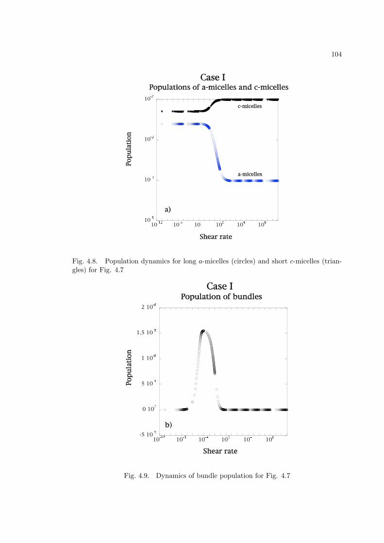
104

Fig. 4.8. Population dynamics for long a-micelles (circles) and short c-micelles (trian-gles) for Fig. 4.7

Fig. 4.9. Dynamics of bundle population for Fig. 4.7

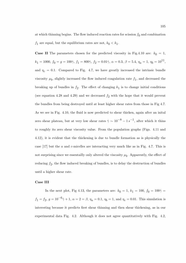
105

at which thinning begins. The flow induced reaction rates for scission f0 and combination

f1 are equal, but the equilibrium rates are not, k0 < k1.

Case II The parameters chosen for the predicted viscosity in Fig.4.10 are: k0 = 1,

k1 = 1000, f0 = g = 100γ, f1 = 800γ, f2 = 0.01γ, α = 0.3, β = 5.4, ηa = 1, ηb = 1011,

and ηc = 0.1. Compared to Fig. 4.7, we have greatly increased the intrinsic bundle

viscosity µb, slightly increased the flow induced coagulation rate f1, and decreased the

breaking up of bundles in f2. The effect of changing k1 is to change initial conditions

(see equation 4.28 and 4.29) and we decreased f2 with the hope that it would prevent

the bundles from being destroyed until at least higher shear rates from those in Fig 4.7.

As we see in Fig. 4.10, the fluid is now predicted to shear thicken, again after an inital

zero shear plateau, but at very low shear rates γ ∼ 10−8 − 1 s−1, after which it thins

to roughly its zero shear viscosity value. From the population graphs (Figs. 4.11 and

4.12), it is evident that the thickening is due to bundle formation as is physically the

case [17] but the a and c-micelles are interacting very much like as in Fig. 4.7. This is

not surprising since we essentailly only altered the viscosity µb. Apparently, the effect of

reducing f2, the flow induced breaking of bundles, is to delay the destruction of bundles

until a higher shear rate.

Case III

In the next plot, Fig 4.13, the parameters are: k0 = 1, k1 = 100, f0 = 100γ =

f1 = f2, g = 10−6γ + 1, α = 2 = β, ηa = 0.1, ηb = 1, and ηc = 0.01. This simulation is

interesting because it predicts first shear thinning and then shear thickening, as in our

experimental data Fig. 4.2. Although it does not agree quantitatively with Fig. 4.2,

106

Fig. 4.10. Predicted normalized viscosity dependence on shear rate. Parameters used:k0 = 1, k1 = 1000, f0 = g = 100γ, f1 = 800γ, f2 = 0.01γ, ηa = 1, ηb = 1011, ηc = 0.01,α = 0.3, β = 5.4.

107

Fig. 4.11. Population dynamics for a-micelles (circles) and c-micelles (triangles) for Fig.4.10.

Fig. 4.12. Dynamics of bundle population for Fig. 4.10.

108

it is in some sense at the opposite end of a spectrum from Fig. 4.7 i.e. both Figs. 4.7

and 4.13 predict both thinning and thickening but in reverse order. There is only one

change in parameters for these figures in the breaking rate of bundles: g = 100γ for Fig.

4.7 whereas g = 10−6γ + 1 for Fig. 4.13. So by decreasing the breaking rate further

from the value used in producing Fig. 4.7, we have pushed the formation of bundles

to a much higher shear rate (Fig. 4.15), and we have stabilized bundle existence by

decreasing the flow dependent breaking rate adding a constant to g. It is not clear that

the added constant has a specific and identifiable role in the population dynamics for

this case. Fig. 4.14 shows that the dynamics of the a and c-micelles have not changed

qualitatively from the previous dynamics with different choices of parameters. So this

is a first approximation to the rheology data for 3.5 mM CPCl / NaSal in Fig. 4.2. As

expected the rise in bundle population is mirrored by a decline in a-micelle population,

visible in Fig. 4.14 near γ ∼ 103 s−1.

We note that although the shear rates at which the thickening occurs and sub-

sequent thinning, this plot (Fig. 4.10) is in amazingly good qualitative agreement with

physically observed results for low concentration wormlike micellar fluids (Figure 1 in

[17]). The increase of viscosity in this plot is over two orders of magnitude, and experi-

mentally thickening is less than a single order of magnitude. Viscosities increase twofold

or threefold in typical experiments on dilute solutions of wormlike micelles, so that by de-

creasing ηb in our simulations we would both recover a more physically accurate rheology

profile, and have a more reasonable value for ηb.

Case IV

109

Fig. 4.13. Predicted viscosity dependence on shear rate. Parameters used: k0 = 1,k1 = 1000, f0 = f1 = f2 = 100γ, g = 10−6γ +1, ηa = 0.1, ηb = 1, ηc = 0.01, α = β = 2.

110

Fig. 4.14. Population dynamics for a-micelles (circles) and c-micelles (triangles) for Fig.4.13

Fig. 4.15. Dynamics of bundle population for Fig. 4.13

111

Finally, we include a plot in which only shear thickening occurs. For Fig. 4.16

the choice of parameters is: k0 = 1, k1 = 100, f0 = 10−6γ, f1 = 10−2γ, f2 = 100γ,

g = 10−4γ, α = 2 = β, ηa = 0.1, ηb = 1, and ηc = 0.01. This choice of parameters a

priori seems like it should give the thickest fluid yet, since the flow-induced coagulation of

c into a is greater than a → c scission and the bundle formation from a is at a greater rate

f2 than either f0 or f1, and the breaking rate of bundles is much lower than the bundle

formation rate. And as we see in Fig. 4.16 the fluid has a constant zero shear viscosity

at low γ followed by shear thickening at a shear rate which is physically reasonable:

γ ∼ 0.1 s−1. Moreover, the value of viscosity increase is perfectly sensible, and the curve

agrees qualitatively with the experimental data shown in Fig. 4.1 for a dilute solution of

1 mM CPCl / NaSal. Here again our choices of parameters result in a bundle formation

which does not decay over a large range of shear rates, but interestingly, after the initial

rise of b near γ ∼ 1000 s−1, there is a secondary increase in b with a coincident decrease

in c-micelle population. In Fig. 4.13 there is also a secondary increase in b population

but there it was fed by a-micelles. This increase in b from c is noticeable in Fig. 4.16

near γ ∼ 104 s−1. Also, both a and c micelle concentration feed into the b population

at the same shear rate, which is not surprising because our choice of parameters is one

that favors a growth at the expense of c, and b growth over a.

While the 2-species model was able to capture shear thickening, it is the rise

and subsequent decrease in viscosity that we associate with SIS formation. Physically

we expect that at high enough shear rates, the bundles will break apart, decreasing

the effective viscosity of the fluid. With the inclusion of the bundle species, the 3-

species model was able to produce the rheology of SIS formation but the 2-species model

112

was not. The sample predictions we have shown are not necessarily characteristic of

all possible predictions, rather they show that the model is able to adress the various

rheological features of wormlike micellar fluids. The 3-species model has therefore been

successful, qualitatively and to a large extent quantitatively, in the sense of capturing

the rheology we set out to reproduce. So far, though, we have examined only steady

state behaviour and in the next chapter time dependence will be included. As we will

see, this will introduce additional and subtle mathematical complexities, which have a

very nice physical interpretation.

113

Fig. 4.16. Predicted viscosity dependence on shear rate. Parameters used: k0 = 1,k1 = 100, f0 = 10−6γ, f1 = 10−2γ, f2 = 100γ, g = 10−4γ, ηa = 0.1, ηb = 1, ηc = 0.01,α = β = 2.

114

Fig. 4.17. Population dynamics for a-micelles (circles) and c-micelles (triangles) for Fig.4.16.

Fig. 4.18. Dynamics of bundle population for 4.16.

115

Chapter 5

Modified Memory:

How to Remember to Forget

5.1 Modified memory

In equation 4.24 for the steady state stresses of the 3-species model, the concen-

tration functions a(t), b(t), and c(t) appear on the outside of the memory integrals, as

weights to the Maxwell stress for each species. Since we were only concerned with the

steady state, concentrations were treated as functions of γ, without time dependence

since we were using limiting values (e.g. limt→∞ a(t)). The point is that we could

regard the concentrations simply as weights, placing them outside the integrals in equa-

tions 4.24. As steady state values, the concentrations could be placed inside or outside

the integrals equally, there was no reason to consider the mathematical impact or phys-

ical difference of this placement. In this chapter, however, we consider time dependent

stresses. As we will see, the two choices of placing the concentrations inside or outside

the memory integral have different physical meanings, both of which are contradicted by

the physical process we model.

We can consider the following cases, which expose an interesting connection be-

tween memory and the breaking and joining of micelles. These kinetic processes are

identified in the concentration functions as a decrease (breaking) or an increase (join-

ing). The cases to consider are the various combinations of increasing or decreasing

116

concentrations, placed inside or outside the memory integral for stress. First suppose

that a(t) is strictly increasing, for example a(t) = t. Then if we write

σa(t0) = a(t0)2η

λ

∫ t0

0e(t′−t0)/λD(t′)dt′, (5.1)

we are effectively remembering that there were a(t0) = t0 micelles at time t0 and at

all previous times. Because the concentration function is not under the integral, we are

weighting the Maxwell stress by a(t0) even as we integrate over the past history of the

rate of strain when there were fewer a-micelles. In this case we are over-counting since

a(t′) < a(t0) for all times t′ < t0.

Next suppose that a(t) is decreasing (due to breaking), say from t = 0 to t0,

and the concentration is placed again outside the memory integral as in equation 5.1.

Computing stress at t0 would use a(t0), and exclude the larger values of a at previous

times. There is no memory of the micelles present in the fluid at earlier times, which

seems like under-counting. However, we are excluding the contribution of micelles which

have converted to another species - equation 5.1 is the stress from a-micelles. Should

we allow micelles, which existed in the past but no longer exist, to still contribute to the

stress?

To answer this let us recall that the way polymers and micelles are believed to

supply stress to the fluid is through their extension, or uncoiling. When their ends

are separated, they act like stretched springs, storing energy and exerting a force on

the nearby fluid. Now imagine instantaneously removing a stretched spring, is there

117

any force left from it? If an a-micelle breaks (presumably instantaneously) into two c-

micelles, then any stress contribution would come from the c-micelles, but the a-micelle

no longer exists, so it cannot continue to stress the fluid. So when any micelle (or

bundle) disappears due to breaking or joining, any stress it was carrying disappears as

well. Therefore, there is no contradiction with placing a decreasing concentration outside

the integral. But a general concentration function (solution to the ODE’s 4.20-4.22) can

decrease over certain times, and increase as well. Putting the concentration outside the

integral would then be physically inaccurate in the general case.

It is certainly possible that when a-micelles break, the new c-micelles (or bundles)

born from a converted a-micelle may carry stress, if the a-micelle broke in a way to create

stretched c-micelles. We do not exclude this possibility, in fact we depend on it. We

assume that some c-micelles will be stretched when they come from broken a-micelles,

and some will be less stretched. Each species in flow will carry stress from the deformation

caused by the flow, and we can consider each member of a species to carry the average

amount of stress caused by flow. Our assumption is that the average amount of stress

in a newly born micelle (or bundle) is equal to the average amount of stress caused

by flow. This means that we need only count how much of a species is present in the

fluid to compute the stress, and we do not need to keep track of how many members of

the species came about by a breaking or joining event. The only stress we exclude are

the stress contributions from micelles which are no longer present in the fluid, but were

perhaps at one time.

118

We next suppose that a(t) should appear under the integral sign. Let a(t) be

increasing from t0 to t1. To compute stress at t1 we would use

σa(t1) =2ηaλa

∫ t1

0a(t) e(t−t1)/λaD(t)dt.

As we integrate over the past history, we are using the past concentration as well. The

integral is “remembering” that we had fewer micelles in the past, which is appropriate

since these micelles still exist at the time we compute stress at t1. So there is no problem

with this scenario.

However, let us take a(t) to be decreasing from say time t1 to t2, with t1 < t2.

With the concentration inside the integral, the formula for stress at t2 would be

σa(t2) =2ηaλa

∫ t2

0a(t′) e(t′−t2)/λaD(t′)dt′.

In this case, as we integrate from 0 to t2, we remember the micelles which existed at

times t < t2, but which have vanished by the time we compute stress at t2! We have

just argued that when they vanish, the stress they were carrying also vanishes, so these

micelles should be excluded from the stress computation.

In general then, it is not correct to have a(t) either outside or inside the integral.

We could resolve this problem if we kept something like the concentration inside the

integral sign but somehow excluded the micelles that broke. So we need to find a function

of time which is almost the concentration but makes our model for the memory of stress

more physically accurate. So rather than use weighted Maxwell stresses, as we could in

119

the steady state case, we now propose stresses of the form

σa(t) =ηaλa

∫ t

0(“Replacement for the concentration a(t)”) e(t′−t)/λaD(t′)dt′, (5.2)

with similar expressions for σb(t) and σc(t).

3 Π

25 Π

27 Π

2

time

0.2

0.4

0.6

0.8

1

Forgetting Broken Micelles

Fig. 5.1. The concentration a(t) is depicted as the dashed curve, while the solid curveis the corrected concentration, which excludes the micelles that grew from t1 = 3π/2 tot2 = 5π/2, and then broke by time t3 = 7π/2.

This raises an interesting point about our course of modelling. That is, we first set

out to model the ability of micelles to exchange mass by having three species of micelle,

and allowing thier concentrations to interact throught the ODE’s 4.20-4.22. We then

used the law of partial stresses to combine the species specific stresses, each given by

the Maxwell equation appropriately weighted with concentration. But we are now faced

again with the process we have already modelled, and we see that this physical property

120

of micelles cannot be decoupled from the stress equation as we have attempted to do by

writing separate ODE’s for it. We must again model breaking and reforming. Whereas

we first used the ODE’s 4.20-4.22 to model what species was in the fluid, we now need

to model how the ability to convert from one species to another effects memory.

Let us consider some examples to motivate our first attempt of determing a physi-

cally relevant “replacement function.” For example, say a(t) increases from t1 = 3π/2 to

t2 = 5π/2, and decreases from t2 to t3 = 7π/2, as in Figure 5.1. If we wish to compute

stress at time t3 = 7π/2, then we need to replace a(t) with a similar function, but which

completely ignores the “bump” ranging from t1 to t3. This means forgetting that the

long micelles created during (t1, t2) ever existed, because they subsequently died over

(t2, t3). To get the stress at time t3 = 7π/2, we should use as a replacement function

the solid curve depicted in Figure 5.1. This curve is only depicted up to 7π/2, since that

is all that is relevant for the memory integral in equation 5.2.

If we had asked for the stress at time t2 = 5π/2, then the micelles (in the previous

example of Figure 5.1) born from 3π/2 to 5π/2 would not yet have been destroyed.

Clearly the solid curve in Figure 5.1 would be unsuitable, and we see immediately that

the “replacement concentration function” depends on the time at which we compute

stress. To make this point more clear we use the following simple examples. Suppose

the concentration a(t) is as depicted by the dashed curve in Figure 5.2. To compute

stress at time π, we would have to ignore the amount of a-micelles that was destroyed

before time π, so the proper replacement concentration would be given by the solid curve

in Figure 5.2. Let us denote this replacement function by R a(π, t), the superscript a

121

Π 3 Πtime

0.2

0.4

0.6

0.8

1Replacement function for ΣaHΠL

Fig. 5.2. The original concentration a(t) is shown as the dashed curve, while the solidcurve is a proposed replacement function for obtaining stress at time π in equation 5.2.

Π 3 Πtime

0.2

0.4

0.6

0.8

1Replacement function for ΣaH3ΠL

Fig. 5.3. The original concentration, a(t) is shown as the dashed curve. Here the solidcure is the replacement function for computing stress (equation 5.2 at time 3π.

122

denoting a-micelles. The stress at π would then be given by

σa(π) =ηaλa

∫ π

0R a(π, t′)e(t′−t)/λaD(t′)dt′. (5.3)

Now suppose, using the same concentration function a(t), that we would like the

stress at time 3π. In this case we would need the replacement concentration shown as

the solid curve in Figure 5.3, which we denote by R a(3π, t). Notice that R a(π, t′) 6=

R a(3π, t′) for all t′ < π.

The three example given in Figures 5.1-5.3 imply that the replacement function

should somehow compare minima of the concentration at different times. More precisely,

to compute stress at time s, we could use the replacement function R a(s, t) defined by

R a(s, t) =

mina(s), a(t) t ≤ s

a(t) t > s,

(5.4)

with similar definitions for bundles and c-micelles. The choice of making R a(s, t) = a(t)

for t > s seems somewhat arbitrary since it does not enter into the stress equation, but

we make this choice to be consistent with a function which we define in the next section.

To compute stress at time s we would then have

σa(s) =ηaλa

∫ s

0R a(s, t)e(t−s)/λaD(t)dt. (5.5)

Equation 5.4 is our first attempt at the replacement function. This definition for Ra(s, t)

was in fact used to produce each of the solid curves in Figure 5.1-5.3.

123

1 2 3 4 5time

1

3

5

RaH2,tL: Replacement function for ΣaH2L

Fig. 5.4. The solid curve is R a(2, t) for the concentration function depicted as thedashed curve.

1 2 3 4 5time

1

3

5

RaH5,tL: Replacement function for ΣaH5L

Fig. 5.5. The solid curve is R a(5, t) for the concentration function depicted as thedashed curve from Figure 5.4.

124

Given the definition in equation 5.4, R a(s, t) is clearly bounded by the actual

concentration function a(t). If it is to eliminate all events in which members of a species

disappear, then the replacement function should also be non-decreasing. Indeed, the way

we identify that an amount of one species has converted to another species is when the

concentration decreases. However, our first attempt in equation 5.4 unfortunately fails

in this respect. Consider a concentration function such as the dashed curve in Figure

5.4. While R a(2, t) is physically accurate (the solid curve in Figure 5.4) in the sense that

it “forgot” about the destroyed micelle population, R a(5, t) is no longer non-decreasing

as shown by the solid curve in Figure 5.5. The replacement function correctly forgot

the micelles destroyed from t = 1 to t = 2 when we compute stress at s = 2, but at

a later time (s = 5) it “forgot to forget” these same destroyed micelles. We need a

new replacement function, one which correctly forgets destroyed micelles, and which will

never again “re-remember” them.

Although equation 5.4 is not suitable to compute stress with, it was presented

for three reasons. First, it is correct for some choices of concentration functions, and

those for which it fails reveal also what exactly needs to be fixed. Second, it serves as

a stepping stone and will make it easier to understand the more complex definition we

present in the next section. Finally, R a(s, t) was our actual first attempt on our way to

defining a final replacement function.

5.2 The time dependent constitutive equation

The task now is to write a physically correct time dependent function which

replaces the concentration functions a(t), b(t), and c(t). The previous section gave us

125

a good start, but we have at least to correct the flaw in equation 5.4 for R a(s, t). In

fact, it is the view that R a(s, t) “forgot to forget” that we use as inspiration for the next

definition for the replacement function. What this phrase refers to is the problem we

exposed with R a(s, t) in Figure 5.5. The problem can be stated by saying that while

R a(2, t) eliminated the micelles that were destroyed from t = 1 to t = 2, R a(5, t) did

not “remember” to eliminate this same amount of micelles. What we need is to use the

information from R a(2, t) when we compute R a(5, t). Indeed, if we can make R a(s, t)

always “remember to forget” that which it forgot before, we will have our non-decreasing,

bounded replacement function. We do this in two steps: first we do it approximately by

asking R a(s, t) to check itself against R a(s− ε, t), then we let ε → 0.

A definition for the replacement function for the concentration a(t) which checks

itself in this way is given by

P aµ

(s, t) =

mina(t), a(s), P aµ

(s− µ, t) 0 ≤ t < s, µ < s

mina(t), a(s) 0 ≤ t < s, µ ≥ s

a(t) t ≥ s ≥ 0.

(5.6)

This function is only defined for s ≥ 0, t ≥ 0, and for all cases we use only µ > 0. The

superscript a denotes the concentration a(t), and again, there are analogous definitions

for P bµ

(s, t) and P cµ

(s, t). The notation is cumbersome so in the sequel we may suppress

the superscript and refer to this simply as Pµ.

Our new function Pµ(s, t) has two variable (and the parameter µ), both of which

represent time, which we now discuss. Recall that the first variable s is regarded as

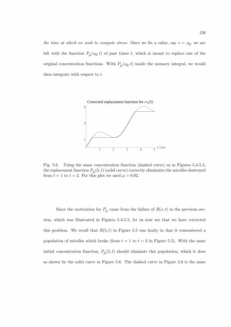
126

the time at which we wish to compute stress. Once we fix a value, say s = s0, we are

left with the function Pµ(s0, t) of past times t, which is meant to replace one of the

original concentration functions. With Pµ(s0, t) inside the memory integral, we would

then integrate with respect to t.

1 2 3 4 5time

1

3

5

Corrected replacement function for ΣaH5L

Fig. 5.6. Using the same concentration function (dashed curve) as in Figures 5.4-5.5,the replacement function Pµ(5, t) (solid curve) correctly eliminates the micelles destroyedfrom t = 1 to t = 2. For this plot we used µ = 0.02.

Since the motivation for Pµ came from the failure of R(s, t) in the previous sec-

tion, which was illustrated in Figures 5.4-5.5, let us now see that we have corrected

this problem. We recall that R(5, t) in Figure 5.5 was faulty in that it remembered a

population of micelles which broke (from t = 1 to t = 2 in Figure 5.5). With the same

initial concentration function, Pµ(5, t) should eliminate this population, which it does

as shown by the solid curve in Figure 5.6. The dashed curve in Figure 5.6 is the same

127

concentration function which was used in Figures 5.4-5.5. The value of the parameter µ

to produce this plot was µ = 0.02.

Before taking the limit as µ → 0, we address the role of the parameter µ. The

difference between equation 5.4 for R(s, t) and equation 5.6 for Pµ is the extra term

Pµ(s − µ, t) in the case when t ≤ s and µ < s. This term is therefore responsible for

correcting the problem with R(s, t), and it serves to iteratively compare Pµ with earlier

versions of itself. So that Pµ(s, t) checks itself against Pµ(s − µ, t), which checks itself

again Pµ(s− 2µ, t), and so on until (s− kµ) ≤ µ. This is how Pµ “remembers to forget”

what it had forgotten in “previous versions of itself.” As soon as (s − kµ) ≤ µ, the

definition of Pµ in equation 5.6 toggles into the second case because we can no longer

subtract µ from the first argument (s−kµ) (both arguments of Pµ must be non-negative).

Toggling into the second case means that we are using exactly our definition of R(s, t)

(equation 5.4). So the function Pµ is not completely correct; if we ask for stress at times

s such that s ≤ µ, we could have a flawed replacement function. As we stated at the

beginning of this section, equation 5.6 is approximate. In the limit as µ → 0, there will

be no values of s for which Pµ toggles into the second case in definition 5.6; this is the

function we actually want. So our next task is to show that the limit of Pµ as µ → 0

exists.

PROPOSITION 5.2.1. The function defined by

P (s, t) = limµ→0

Pµ(s, t)

exists for each point (s, t) such that s ≥ 0 and t ≥ 0.

128

Proof:

We will show that for each point (s, t) with s ≥ 0 and t ≥ 0, and any convergent

sequence µn → 0, the sequence Pµn(s, t) is Cauchy.

Case i) Both s and t are fixed, and 0 ≤ t < s. First we will go out far enough in

the sequence of µn to have Pµntoggle into the first case in definition 5.6 at (s, t) and

(s − µ, t). So let N1 be such that ∀ n > N1 we have 3µn < s and 2µn < (s − t), so

that µn < (s − 2µn) < (s − µn) and t < (s − 2µn) < (s − µn). For each n > N1, the

Archimedean Order Property and Completeness of R, guarantees that we can find an

integer kn such that

s− (kn + 1)µn ≤ t ≤ (s− knµn). (5.7)

For each n > N1, we can also find jn ∈ Z+ with

s− (jn + 1)µn ≤ µn ≤ (s− jnµn). (5.8)

So as long as n > N1, we have the first case in the definition of Pµ, i.e. Pµn(s, t) =

mina(t), a(s), Pµn(s − µn, t) as well as Pµn

(s − µn, t) = mina(t), a(s), Pµn(s −

2µn, t).

If jn < kn, then Pµn(s − (jn + 1)µn, t) = mina(t), a(s). If kn ≤ jn, then

Pµn(s − (kn + 1)µn, t) = a(t). Without loss of generality, we may assume kn ≤ jn, to

129

get

Pµn(s, t) = mina(t), a(s), Pµn

(s− µn, t)

Pµn(s− µn, t) = mina(t), a(s− µn), Pµn

(s− 2µn, t)

·:

Pµn(s− knµn, t) = mina(t), a(s− knµn), Pµn

(s− (kn + 1)µn, t)

= mina(t), a(s− knµn),

and hence

Pµn(s, t) = mina(t), a(s), a(s− µn), a(s− 2µn), ..., a(s− knµn). (5.9)

If it were the case that jn < kn, then we would still end up with equation 5.9 for

Pµn(s, t), but with jn replacing kn.

Note that the concentration functions a(t), b(t), and c(t) are solutions to ODE’s

4.20-4.22, so we may assume that they are each continuous. Since the interval [t, s] ⊂ R

is compact, the concentrations are uniformly continuous on [t, s]. Then for any given ε,

find δ1 such that for x, y ∈ [t, s],

‖x− y‖< δ1 =⇒ ‖a(x)− a(y)‖< ε/2.

Before proceeding, we will need the following lemma.

130

LEMMA 5.2.2. “Cramping the µn” Suppose we are given µn, µm ∈ (0, δ1/4), and

0 ≤ t < s. Let kn and km be as defined as in equation 5.7. If α ∈ Z with 0 ≤ α ≤ kn,

then there exists a γ ∈ Z with 0 ≤ γ ≤ km such that ‖(s− γµm)− (s− αµn)‖< δ1/2.

Proof:

If α = 0, then choose γ = 0 and we are done. We next assume that s− αµn < s.

Find the largest γ ∈ Z, γ ≥ 0, such that (s−αµn ) < s−γµm. If (s−γµm)−(s−αµn) ≥

δ1/4, then s− (γ + 1)µm− (s−αµn) = (s− γµm)− (s−αµn)−µm ≥ δ1/4 > 0, which

contradicts the definition of γ. So we conclude that (s − γµm) − (s − αµn) < δ1/2.

Finally, since (s− γµm) > (s− αµn) > t, then by the definition of km (equation 5.7),

it must be that γ ≤ km. Lemma 5.2.2 is now proved.

We are now ready to prove Pµn(s, t) is Cauchy. So let ε > 0 be given. We need to

find an N ∈ Z+ such that whenever n, m > N , we have ‖Pµn(s, t)−Pµm

(s, t)‖< ε. Take

N > N1 (defined above) such that ∀ n > N , we have ‖µn ‖< δ1/4, using the Lemma.

Using equation 5.9, we know it may happen that for some n, m > N , either one or

both of Pµn, Pµm

may be equal to a(t). If both are equal to a(t), then clearly we have

‖Pµn(s, t) − Pµm

(s, t) ‖< ε. Suppose Pµn(s, t) = a(t), while Pµm

(s, t) = a(s − βµm),

with β ∈ Z and 0 ≤ β ≤ km, with km as defined above. If ‖ a(t) − a(s − βµm) ‖> ε,

then we will obtain a contradiction. Since Pµm(s, t) = a(s − βµm), we know from

equation 5.9 that a(s − βµm) ≤ a(t). From Lemma 5.2.2, we can find γ such that

‖(s− γµn)− (s− βµm)‖< δ1/2, with 0 ≤ γ ≤ kn. Since Pµn(s, t) = a(t), we know that

a(t) < a(s− γµn). Hence

‖a(t)− a(s− βµm)‖= a(t)− a(s− βµm) < a(s− γµn)− a(s− βµm) < ε/2 < ε.

131

But then this contradicts our assumption. Therefore, for all n,m > N , if Pµn(s, t) = a(t),

and Pµm(s, t) = a(s− βµm), then ‖Pµn

(s, t)− Pµm(s, t)‖< ε.

We next suppose that with n, m > N , we have Pµn(s, t) = a(s − αµn) with

0 ≤ α ≤ kn, and Pµm(s, t) = a(s− βµm) with 0 ≤ β ≤ km. Without loss of generality,

we may assume that

a(s− αµn) < a(s− βµm).

So find γ ∈ Z, 0 ≤ γ ≤ km, such that ‖ (s − αµn) − (s − γµm) ‖< δ1/2. Then

since Pµm(s, t) = a(s− βµm), we know that a(s− γµm) ≥ a(s− βµm). Therefore,

‖a(s−βµm)−a(s−αµn)‖= a(s−βµm)−a(s−αµn) ≤ a(s−γµm)−a(s−βµn) < ε/2.

This concludes the proof of propostion 5.2.1 for case i) in which 0 ≤ t < s.

Case ii) Both s and t are fixed, with t ≥ s. This case is trivial since Pµn(s, t) =

Pµm(s, t) = a(t).

Since we are taking the limit as µ → 0, we do not have to check the case where

0 ≤ t < s and µ ≥ s. For a fixed s, we just go far enough out in the sequence that we

are guaranteed all µn < s. This concludes the proof to proposition 5.2.1.

So for each concentration function a(t), b(t), and c(t), our model uses a replace-

ment concentration given by the limit functions we now know exist. We denote these

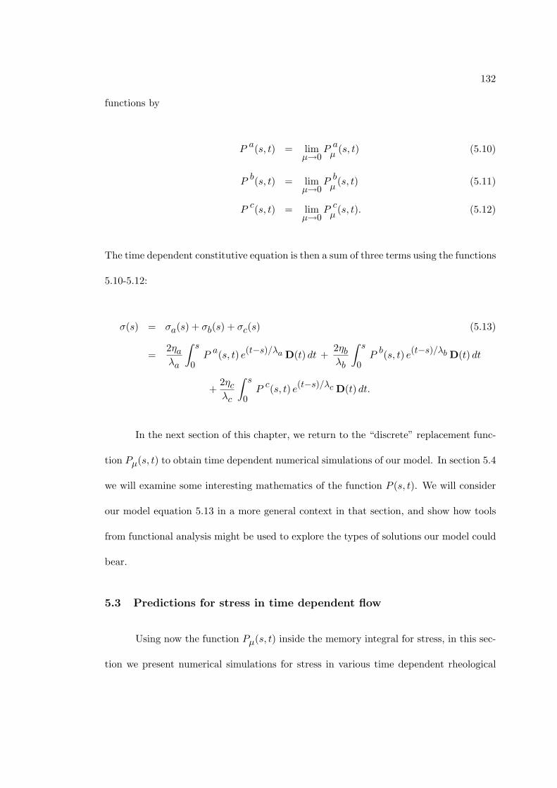
132

functions by

P a(s, t) = limµ→0

P aµ

(s, t) (5.10)

P b(s, t) = limµ→0

P bµ

(s, t) (5.11)

P c(s, t) = limµ→0

P cµ

(s, t). (5.12)

The time dependent constitutive equation is then a sum of three terms using the functions

5.10-5.12:

σ(s) = σa(s) + σb(s) + σc(s) (5.13)

=2ηaλa

∫ s

0P a(s, t) e(t−s)/λa D(t) dt +

2ηbλb

∫ s

0P b(s, t) e(t−s)/λb D(t) dt

+2ηcλc

∫ s

0P c(s, t) e(t−s)/λc D(t) dt.

In the next section of this chapter, we return to the “discrete” replacement func-

tion Pµ(s, t) to obtain time dependent numerical simulations of our model. In section 5.4

we will examine some interesting mathematics of the function P (s, t). We will consider

our model equation 5.13 in a more general context in that section, and show how tools

from functional analysis might be used to explore the types of solutions our model could

bear.

5.3 Predictions for stress in time dependent flow

Using now the function Pµ(s, t) inside the memory integral for stress, in this sec-

tion we present numerical simulations for stress in various time dependent rheological

133

flows. Our model accounts for the reversible scission reactions in the stress computation,

and here we show how it works in live examples. In the first choice of flow, in addition

to stress predictions we show the dynamics of the concentration functions and the corre-

sponding replacement functions Pµ, as an initiation to the details of the model. We also

show how using Pµ differs from the models which do not include the scission reactions of

micelles, namely the approach of using the original concentration functions placed inside

or outside the integral, as well as the Maxwell model. Parameter choices differ for the

different flows we test, but for all of the figures in this section some paramters are held

fixed. These parameters are: τ = 100, V = 1, and M = 0.01.

5.3.1 Linearly ramping shear

All of the flows we consider are time dependent simple shear flows, and the first

that we consider is given by γ(t) = t. For this flow we show several plots (Figures

5.7-5.14), for which we use the same parameter values: γ(t) = t, µ = 0.01, k0 = 102,

k1 = 103, f0(γ) = 0, g(γ) = 10−3γ, f1(γ) = 104γ, f2 = 106γ, α = β = 2, ηa = 103,

ηb = 10, ηc = 10−3, and λa = λb = λc = 1. Since this is our first time dependent flow, it

is the first time we can see how our model (equations 4.20-4.22 with 5.13) works. Since

it differs from the Maxwell model in its modification of the concentration functions, we

begin by examining the dynamics of the three species in Figures 5.7-5.9. Shown also in

each of these plots are samples of our modified memory function Pµ.

In Figure 5.7 we see that the population of a-micelles peaks quickly and then

decays to a plateau value of roughly limt→∞ a(t) ∼ 0.00011. When we compute stress

at times near s ∼ 10 − 20, the modified concentration function P aµ

will be constant

134

0 5 10 15 20

0.00025

0.0005

0.00075

0.001

0.00125

0.0015

Dynamics of a-micelles with PΜaHs,tL

Fig. 5.7. The dynamics of a-micelles is shown as the thick dashed curve. Plots ofP a

µ(0.6, t), P a

µ(1.7, t), and P a

µ(6.5, t) are also shown as solid curves, with µ = 0.01. The

paramaters used for these dynamics are the same for the stress plots 5.10-5.14 whichare: γ(t) = t, k0 = 102, k1 = 103, f0(γ) = 0, g(γ) = 10−3γ, f1(γ) = 104γ, f2 = 106γ,α = β = 2, ηa = 103, ηb = 10, ηc = 10−3, and λa = λb = λc = 1.

0 5 10 15 200

0.00025

0.0005

0.00075

0.001

0.00125

0.0015

Dynamics of bundles with PΜbHs,tL

Fig. 5.8. The dynamics of bundles is shown as the thick dashed curve. A plot ofthe modified concentration P b

µ(6.5, t) is shown as the solid curve (µ = 0.01), which is

identical to the concentration function b(t) up to that time since b(t) is monotonicallyincreasing. Parameter values are the same as for Figure 5.7.

135

and approximately equal to the plateau value limt→∞ a(t), such as shown by the plot

of P aµ

(6.5, t). At smaller times, before any a-micelles convert to bundles or break into

c-micelles, P aµ

will be equal to a(t). When a(t) starts decreasing, P aµ

correctly excludes

the amount of a-micelles lost to another species, as shown by the plots of P aµ

(0.6, t) and

P aµ

(1.7, t).

0 5 10 15 200

0.002

0.004

0.006

0.008

0.01Dynamics of c-micelles with PΜ

cHs,tL

Fig. 5.9. The dynamics of c-micelles is shown as the thick dashed curve. Plots ofP c

µ(1.0, t) and P c

µ(3.0, t) are shown as solid curves, both are constant since the concen-

tration function c(t) is monotonically decreasing. Parameter values are the same as forFigure 5.7.

Evidently, the a-micelle decrease is feeding the bundle population b(t), shown in

Figure 5.8 (since the c-micelle concentration is decreasing for all times in Figure 5.9).

For bundles, which begin at b(0) = 0, there is a monotonic increase, so that for all s and

t we have P bµ

(s, t) = b(t). A sample of the modified concentration is given in Figure 5.8

by P bµ

(6.5, t) as the solid curve, which follows b(t) perfectly from t = 0 to t = 6.5 as it

136

should. The c-micelle decrease in Figure 5.9 must be feeding the early a-micelle increase.

This makes sense since we have chosen k0 < k1, f0(γ) = 0 while f1(γ) = 104γ (see the

schematic of reaction rates in Figure 4.4). The plateau value for c is similar to that of

a: limt→∞ c(t) ∼ 0.00015. We must remember that these values are mole fractions, and

with our choices of M = 0.01 and V = 1, they are each always less than M · V = 0.01,

obeying the non-dimensional conservation of mass (equation 4.19 multiplied by V on

both sides).

With these as population dynamics for the shear flow γ(t) = t, the stress given

by equation 5.13 is shown in Figure 5.10. In this Figure, in which stress is plotted

against time, the stress increases as we expected since γ is increasing. The effect of

the replacement function is best seen when we compare Figure 5.10 with the stress

prediction of the Maxwell model for the same flow (γ(t) = t), given in Figure 5.11. We

also compare our prediction with predictions of two other flawed models: the first model

comes from adding the Maxwell stresses for each of the three species with the respective

concentration function placed outside the memeory integral, the second model places the

concentration functions inside the integral. In other words, the first model is the sum of

equation 5.1 for the three species, this gives the “outside the integral” prediction (Figure

5.12). Moving the concentration functions to the inside of equation 5.1, and summing

the contribution of each species gives the “inside the integral” prediction seen in Figure

5.13.

Each of the Figures 5.10-5.13 shows an increasing stress. Our model prediction

in Figure 5.10 gives a significantly different prediciton from the Maxwell model, but is

close to the “inside” and even closer to the “outside” prediction. From the resolution

137

0 2 4 6 80

0.2

0.4

0.6

0.8

1

1.2

Time dependent shear stress, Γ =t

Fig. 5.10. Time dependent stress prediction using our model (equation 5.13) for shearflow with shear rate γ(t) = t.

0 2 4 6 80

2000

4000

6000

8000

Time dependent Maxwell stress, Γ =t

Fig. 5.11. Time dependent stress prediction of the Maxwell model for the same shearflow used in Figure 5.10. Parameter values are the same as for Figure 5.7.

138

0 2 4 6 80

0.2

0.4

0.6

0.8

1

1.2

Outside the integral, Γ =t

Fig. 5.12. Time dependent stress with concentration functions inside the Maxwellmemory integral, in the same shear flow used in Figure 5.10.Parameter values are thesame as for Figure 5.7.

0 2 4 6 80

0.2

0.4

0.6

0.8

1

1.2

Inside the integral, Γ =t

Fig. 5.13. Time dependent stress with concentration functions outside the Maxwellmemory integral, in the same shear flow used in Figure 5.10. Parameter values are thesame as for Figure 5.7.

139

of the plots, it seems Figures 5.10 and 5.12 are identical. However, let us understand if

they should be the same or not from the dynamics of the concentration functions and

our understanding of the function Pµ. Since the function c(t) for this flow is strictly

decreasing, for any s0 we have P cµ

(s0, t) = c(s0). Since it is constant it can be moved to

the outside of the integral, so that σc(s0) is the same whether we use P cµ

or simply use

c(s0) outside the integral.

The concentration of a-micelles is also decreasing except very early where it is

increasing. When a(t) has decreased past a(0), P aµ

(s0, t) = a(s0) is constant for the

stress computation and can be pulled out of the integral as well. Before it decreases past

a(0) though, using the concentration outside the integral will be overcounting, so it the

should report values larger than our model. Since the bundle population is increasing

for all time, placing b(s) outside the integral will again overcount and will give a larger

contribution to stress than σb(s) in our model using P bµ

(s, t). So we should expect that

placing the concentrations outside the integral is actually giving larger stresses than our

model. We have plotted the difference of the stresses for these two approaches in Figure

5.14. More precisely, Figure 5.14 is the logarithm (base 10) of the percentage that the

“outside the integral” approach is greater than the corrected prediction given by our

model.

The fact we could use a logarithmic scale means that all stress values obtained

from the “outside” approach are larger than those we obtain with our model. This

confirms our expectation that we overcount by placing the concentrations outside the

memory integral. We also note that the difference is as great as ∼ 11%! The error is

greatest for small times, which makes it more significant. The reason for this is that

140

0 2 4 6 8

-1

-0.5

0

0.5

1

1.5Log of the Percentage Difference, Γ =t

Fig. 5.14. The logarithm (base 10) of the difference of stress values between values fromFig. 5.10 and 5.12, as a percentage of the predicted values in Fig. 5.10 (obtained fromequation 5.13). As expected, the values from Fig. 5.12 are consistently greater thanthose obtained from our model.

in transient rheology tests on non-Newtonian fluids, there is sometimes a “stress over-

shoot” [30, 3], meaning stress peaks and then decreases to its steady value, much like

the population of a-micelles in Figure 5.7. However, in the case of wormlike micelles,

a second transient (“sigmoidal decay”) is sometimes seen in which stress decays more

slowly and does not begin at the high peak of a typical stress overshoot [30]. Our

model is predicting a smaller stress than when the concentrations are placed outside

the integrals, especially where stress overshoots occur, and could therefore be avoiding a

spurious report of a stress overshoot that a weighted Maxwell model would predict. The

inclusion of Pµ in the integral is allowing a second mechanism of stress relaxtion (due

to breaking), whereas a weighted Maxwell model can relax stress only through fading

memory.

141

5.3.2 Oscillatory shear flow

The next flow we consider is an oscillatory shear flow, a standard rheological

test [47]. For each of Figures 5.15-5.21 the parameters values are: µ = 0.01, k0 = 1,

k1 = 100, f0(γ) = 102|γ|, g(γ) = 10−6|γ|, f1(γ) = 10−2|γ|, f2 = 102|γ|, α = β = 2,

ηa = 102, ηb = 104, ηc = 10−2, and λa = λb = λc = 1. The shear rate for Figure 5.15

is γ(t) = 0.01 cos(t), and for Figure 5.16 we use γ(t) = 0.1 cos(t). For the remaining

Figures 5.17-5.21 the shear rate is γ(t) = cos(t).

The first three Figures 5.15-5.17 are predictions of our model for the time depen-

dent stress in shear flow with increasing amplitude of oscillation in the shear rate. It is

not surprising that the stress is oscillating since we are applying an oscillating flow. It is

very interesting that as we increase the strain - which is the amplitude of the shear rate

- the symmetry breaks. The Maxwell model predicts no such effect, as we see in Figure

5.18 for the same strain as used in Figure 5.17. So for this flow too our model is showing

considerable difference with the Maxwell model.

Whereas in the previous section, with flow γ(t) = t, our model predictions in

Figure 5.10 were similar to those obtained using the “outside the integral” model (Figure

5.12), for oscillatory shear the “outside the integral” approach predicts stress which

is extremely different from the other model predictions (Figure 5.19). However, the

“inside the integral” model predicts a stress, shown in Figure 5.20, which is apparently

very similar to our model predictions in Figure 5.17. We again provide a plot of the

difference between the values in these figures to reveal quantitatively the error of using

the actual concentration functions inside the integral. The values shown in Figure 5.21

142

0 5 10 15 20

-0.1

-0.05

0

0.05

0.1

Time dependent shear stress, Strain=0.01

Fig. 5.15. Model prediction (equation 5.13) for shear stress in oscillatory shear flowplotted against time. Here γ = 0.01 cos(t), and parameter values are: µ = 0.01, k0 = 1,k1 = 100, f0(γ) = 102|γ|, g(γ) = 10−6|γ|, f1(γ) = 10−2|γ|, f2 = 102|γ|, α = β = 2,ηa = 102, ηb = 104, ηc = 10−2, and λa = λb = λc = 1.

0 5 10 15 20

-0.04

-0.02

0

0.02

0.04

0.06Time dependent shear stress, Strain=0.1

Fig. 5.16. Prediction of our model (equation 5.13) in oscillatory shear with shear rateγ(t) = 0.1 cos(t). All parameter values are the same as in in Figure 5.15. With anincrease in the amplitude of shear rate, a slight asymmetry develops in the oscillatingstress.

143

0 5 10 15 20

-0.005

0

0.005

0.01Time dependent shear stress, Strain=1

Fig. 5.17. Prediction of our model (equation 5.13) in oscillatory shear flow with γ(t) =cos(t). Parameter values are the same as those in Figures 5.15 and 5.16. At this higheramplitude oscillatory shear rate the asymmetry is much more pronounced than in Figure5.16.

0 5 10 15 20

-75

-50

-25

0

25

50

75

100Time dependent Maxwell stress, Strain=1

Fig. 5.18. Maxwell model prediction for shear stress in oscillatory shear flow with shearrate γ(t) = cos(t). Values of parameters are identical to those used in Figures 5.15-5.17.The asymmetry in Figure 5.17 (which uses the same strain) is absent from the Maxwellprediction.

144

0 5 10 15 20

-0.04

-0.02

0

0.02

0.04

Outside time dependent stress, Strain=1

Fig. 5.19. Prediction for time dependent shear stress in oscillatory shear flow usingconcentration functions on the outside of the memory integral. Here γ(t) = cos(t) andall parameter values are the same as in Figures 5.15-5.18.

0 5 10 15 20

-0.005

0

0.005

0.01Inside time dependent stress, Strain=1

Fig. 5.20. Prediction for time dependent shear stress in oscillatory shear flow using theconcentration functions on the inside of the memory integral. Here γ(t) = cos(t) and allparameter values are the same as in Figures 5.15-5.19.

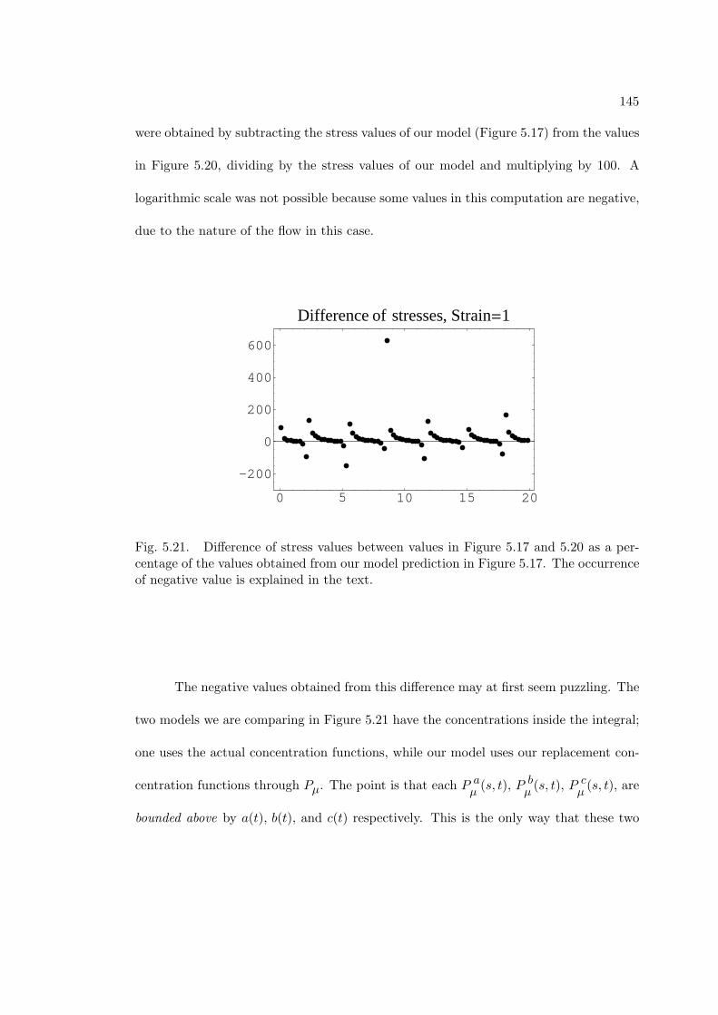
145

were obtained by subtracting the stress values of our model (Figure 5.17) from the values

in Figure 5.20, dividing by the stress values of our model and multiplying by 100. A

logarithmic scale was not possible because some values in this computation are negative,

due to the nature of the flow in this case.

0 5 10 15 20

-200

0

200

400

600

Difference of stresses, Strain=1

Fig. 5.21. Difference of stress values between values in Figure 5.17 and 5.20 as a per-centage of the values obtained from our model prediction in Figure 5.17. The occurrenceof negative value is explained in the text.

The negative values obtained from this difference may at first seem puzzling. The

two models we are comparing in Figure 5.21 have the concentrations inside the integral;

one uses the actual concentration functions, while our model uses our replacement con-

centration functions through Pµ. The point is that each P aµ

(s, t), P bµ

(s, t), P cµ

(s, t), are

bounded above by a(t), b(t), and c(t) respectively. This is the only way that these two

146

models differ, so how could using the functions Pµ yield a stress greater than we ob-

tain using the actual concentrations? The answer is in the flow we have chosen, namely

γ(t) = cos(t), which becomes negative periodically. In the computation of stress, the

memory integral includes the values of the flow for all times less than or equal to the

time at which stress is computed. It will therefore include the negative values of γ(t),

and since the actual concentration, for example a(t), is greater than or equal to its coun-

terpart P aµ

(s, t), we will obtain values of stress which are smaller in magnitude by using

the “inside the integral” model. So even when both models predict a positive stress,

our model can predict a smaller positive stress than that obtained by using the actual

concentration functions.

The error reported in Figure 5.21 is substantial, sometimes over 100% , and more

than 600% near t = 10. While the stress prediction from using the “inside” approach

is qualitatively similar to the predictions of our model, the values in Figure 5.21 give a

clear indication that if we simply place the concentrations inside the Maxwell memory

integral we will obtain false values for stress when using a population model for wormlike

micellar fluids.

5.3.3 Thixotropic loop: Linearly ramping up and down

The flow we consider here is one used in a very interesting rheological test, called

a thixotropic loop [83]. The viscoelasticity in complex fluids is often used synonymously

with “memory”, meaning the fluids remember that they were recently stressed or ex-

perienced a strain. A thixotropic loop study investigates the effect of this macroscopic

147

memory in simple shear flow in an important way. While Newtonian fluids have a con-

stant viscosity, non-Newtonian fluids can have a viscosity which changes, for example

with shear rate in simple shear flow, as in Figures 4.1-4.3 in Chapter 4. It is commonly

said that a non-Newtonian fluid has a viscosity which depends on shear rate, but even

more is true. There is no single viscosity value at a given shear rate, but rather it can

depend on the prior history of deformation. This is known as hysteresis and can occur

in non-Newtonian fluids [83].

In this section we use a simple shear flow with a first increasing then decreasing

shear rate: γ(t) = t if t ≤ 5, and γ(t) = 5 − t if 5 ≤ t ≤ 10. When the shear rate is

decreasing from γ = 5 to γ = 0, we can compare to the values of stress when the shear

rate was increasing from γ = 0 to γ = 5. In this way we obtain a prediction of the

hysteresis in reported values of stress. This test is an example of a “thixotropic loop”, so

called because it is typical to see higher stress at a given shear rate when γ is decreasing

than when it was increasing.

The parameter values used to produce Figures 5.22-5.26 are: µ = 0.01, k0 = 102,

k1 = 103, f0(γ) = 0, g(γ) = 10−3γ, f1(γ) = 104γ, f2 = 106γ, α = β = 2, ηa = 103,

ηb = 10, ηc = 10−3, and λa = λb = λc = 1. In Figure 5.22 the squares denote stress

values at a given shear rate when γ is (linearly) increasing. Upon reaching a shear rate of

γ = 5, the rate decreases linearly back to γ = 0, with stress values given by the triangles

in Figure 5.22. The fact that the stresses at a given shear rate do not coincide is a

prediction of history dependence. The shape of the curve in Figure 5.22 makes physical

sense. By increasing the flow rate, the fluid becomes more stressed, and when the shear

rate begins to decrease, the built up stress needs time to dissipate. The values of stress

148

0 1 2 3 4 50

0.01

0.02

0.03

0.04Thixotropic loop

Fig. 5.22. Time dependent shear stress prediction of our model equation 5.13 in athixotropic loop. Parameter values used are: µ = 0.01, k0 = 102, k1 = 103, f0(γ) = 0,g(γ) = 10−3γ, f1(γ) = 104γ, f2 = 106γ, α = β = 2, ηa = 103, ηb = 10, ηc = 10−3, andλa = λb = λc = 1. Stress values obtained while γ is increasing are given as squares, thetriangles denote stress values when the shear rate is decreasing.

0 1 2 3 4 50

50

100

150

200

250

300Maxwell thixotropic loop

Fig. 5.23. Maxwell model prediction for shear stress in a thixotropic loop using thesame time dependent shear rate as in Figure 5.22. All paramter values used to obtainthe values in this plot are the same as in Figure 5.22. The Maxwell model predicts amuch greater shear thickening effect than our model (equation 5.13) shown in Figure5.22. Stress values obtained while γ is increasing are given as squares, the trianglesdenote stress values when the shear rate is decreasing.

149

0 1 2 3 4 50

0.01

0.02

0.03

0.04Outside the integral thixotropic loop

Fig. 5.24. Prediction of shear stress in a thixotropic loop using the concentrationfunctions outside the memeory integral. The shear rate and all parameter values usedare the same as those used to produce the values in Figure 5.22 and 5.23. Stress valuesobtained while γ is increasing are given as squares, the triangles denote stress valueswhen the shear rate is decreasing.

0 1 2 3 4 50

0.02

0.04

0.06

0.08

0.1Inside the integral thixotropic loop

Fig. 5.25. Predicted shear stress values in a thixotropic loop study. The shear rate andall parameter values used are the same as those used to produce the values in Figure5.22-5.24.Stress values obtained while γ is increasing are given as squares, the trianglesdenote stress values when the shear rate is decreasing.

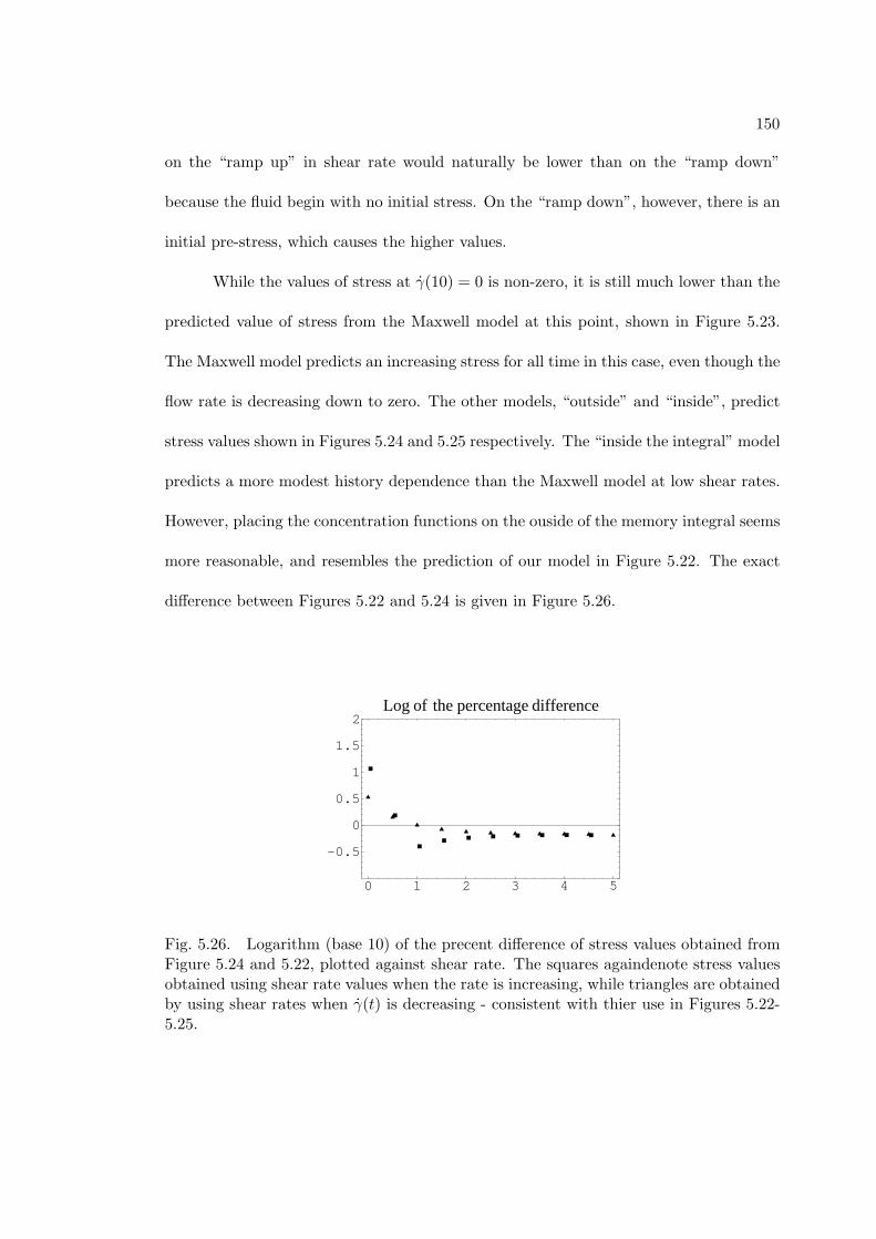
150

on the “ramp up” in shear rate would naturally be lower than on the “ramp down”

because the fluid begin with no initial stress. On the “ramp down”, however, there is an

initial pre-stress, which causes the higher values.

While the values of stress at γ(10) = 0 is non-zero, it is still much lower than the

predicted value of stress from the Maxwell model at this point, shown in Figure 5.23.

The Maxwell model predicts an increasing stress for all time in this case, even though the

flow rate is decreasing down to zero. The other models, “outside” and “inside”, predict

stress values shown in Figures 5.24 and 5.25 respectively. The “inside the integral” model

predicts a more modest history dependence than the Maxwell model at low shear rates.

However, placing the concentration functions on the ouside of the memory integral seems

more reasonable, and resembles the prediction of our model in Figure 5.22. The exact

difference between Figures 5.22 and 5.24 is given in Figure 5.26.

0 1 2 3 4 5

-0.5

0

0.5

1

1.5

2Log of the percentage difference

Fig. 5.26. Logarithm (base 10) of the precent difference of stress values obtained fromFigure 5.24 and 5.22, plotted against shear rate. The squares againdenote stress valuesobtained using shear rate values when the rate is increasing, while triangles are obtainedby using shear rates when γ(t) is decreasing - consistent with thier use in Figures 5.22-5.25.

151

Shown in Figure 5.26 is the logarithm (base 10) of the percentage that the “out-

side” approach is greater than the values obtained by our model. Our use of the logarithm

means that the “outside” stress predictions are always greater than those given by our

model using the modified concentration functions. The difference in this case is greatest

at the lowest shear rates. The error here again is not at all negligible; it is more than

10% at small shear rates.

5.3.4 Concluding remarks on time dependent stress predictions

We began to build our model with the idea of modifying the Maxwell model

with small changes but sufficient to accomodate the physics of wormlike micelles. The

results of the three time dependent simple shear flows we have considered show a definite

difference between our model and the Maxwell model. The model we have put forth

in equation 5.13 and the ODE’s 4.20-4.22, corrects the Maxwell model in the case of

wormlike micelles, by adjusting the memory kernel to forget “broken micelles”. It is

physically inaccurate to place the concentrations inside or outside the memory integral,

and we have solved this problem by defining the functions Pµ. By including the ability

to exchange mass among species, and the effect this has on memory, into the Maxwell

model, we have produced a new model, for both steady and time dependent shear flow.

Summarizing the results for the different flow types, we have found that for both

the linear ramp and the thixotropic loop tests, the “outside the integral” model had

predictions closest to our model with Pµ. For the oscillatory shear flow, however, it

was the “inside the integral” model which came closest. Placing the concentrations

on the outisde can account for breaking events if the concentration is monotonically

152

decreasing. For monotincally increasing concentrations, our function Pµ reduces to the

actual concentration. This suggests that in both the linear ramp and thixotropic loop,

the breaking events occurred on a timescale comparable to the relaxation time, so that

our model could be approximated by having the concentrations outside the integral. For

oscillatory shear, the populations must be oscillating, so that there are both combing

and breaking events. With the concentrations inside the integral, we are overcounting

as shown in Figure 5.21, but evidently the frequent breaking events must be diminishing

this effect, so that the prediction is qualitatively similar to our model.

Although the constitutive equation we have written (equation 5.13) is meant only

for the shear component of stress, we can propose the same model for the full stress

tensor as well. Allowing σ to represent the full stress tensor, the constitutive equation

would still be given by equation 5.13, with the understanding that to compute the ijth

component of σ one must use the ijth component of the rate of strain tensor D.

5.4 Memory integrals and the Fredholm Alternative

In this final section we present material and results which are somewhat specu-

lative. We attempt to exploit an interesting application of ideas in functional analysis

to our model equation 5.13 coupled to the ODE’s 4.20-4.22. After first describing the

problem to be solved, we present the mathematical tools that might be capable of find-

ing a solution. We then give some inital results we have obtained toward this end. The

problems with this approach are also addressed, and we suggest methods in which they

might be handled.

153

5.4.1 The idea of an inverse constitutive equation

While constitutive equations are often thought of as a way to solve determine the

stress in a particular flow field, in this section we consider equation 5.13 from another

point of view. In the following sections we consider the inverse problem, i.e. given a

stress σ, is there a flow u with gradient D which satisfies our model given by equation

5.13 with the given σ.

The motivation for this question comes mainly from interesting rheology of worm-

like micellar fluids. During simple shear flow, wormlike micellar fluids can develop in-

homogeneities and structures larger than wormlike micelles [17, 40, 85, 86]. During a

rheology experiment, these new structures can cause the fluid to “band” [86] into two

seperate fluids moving at different speeds within the chamber holding the fluid sample.

Structures forming in regular patterns have also been observed, which move through

the fluid during experiments [40]. Such phenomena change the velocity gradients in the

fluid, turning an intial homogeneous, viscometric flow such as simple shear flow, into

something more complicated which is no longer pure shear.

The question we ask is whether for a given stress σ(t), there exists a solution

to equation 5.13, i.e. a flow D, which is smooth for only a finite amount of time, and

eventually develops singularities. More ambitious projects would include a classification

of those stresses σ for which C∞ solutions exist, those for which there are no smooth or

even continuous solutions.

We do not answer these questions here, rather we show how useful tools from

functional analysis might yield answers. We next include a review of theorems and

154

definitions if only to establish notation and nomenclature. We then present the results

we have obtained that show our model in equation 5.13 enjoys some key properties that

make it amenable to some of the powerful tools of Fredholm Theory.

5.4.2 Integral equations and Fredholm theory

Let K be a linear operator acting on a Hilbert space H, K : H → H. Recall that

the norm of K is defined as ‖K ‖= inf‖f‖=1 ‖Kf ‖, in which the norms of f and Kf use

the norm on H. In other words, since K is bounded, ‖Kf ‖≤ M ‖ f ‖ for each f ∈ H,

and then ‖K ‖ is the infimum of all such M . An operator is compact if it maps bounded

sets to sets which are sequentially compact. A set is sequentially compact if any sequence

of points, which all belong to the set, has a convergent subsequence. A standard text

containing definitions and standard proofs is Keener [87].

The operators we will be interested in are integral operators acting on functions

in the Hilbert space L2[0, T ], where a ∈ R is a (large) constant. If u ∈ L2[0, T ], then for

an integral operator on L2[0, T ] of the form:

Ku (x) =∫ T

0k(x, y)u(y)dy, (5.14)

is said to have kernel k(x, y). Given a kernel k(x, y), there is an associated integral

operator on L2[0, T ] is simply given by equation 5.14.

We would now like to construct an integral operator using a kernel generated by

P (s, t), dropping the superscript which denotes one of the concentration functions a(t),

b(t), or c(t). For the present discussion, we limit ourselves to any single concentration

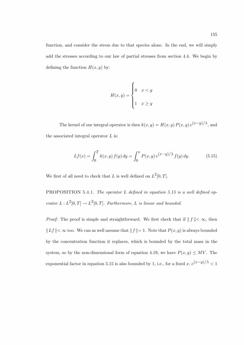
155

function, and consider the stress due to that species alone. In the end, we will simply

add the stresses according to our law of partial stresses from section 4.4. We begin by

defining the function H(x, y) by:

H(x, y) =

0 x < y

1 x ≥ y

The kernel of our integral operator is then k(x, y) = H(x, y)P (x, y) e(x−y)/λ, and

the associated integral operator L is:

Lf(x) =∫ T

0k(x, y) f(y) dy =

∫ x

0P (x, y) e(x−y)/λ f(y) dy. (5.15)

We first of all need to check that L is well defined on L2[0, T ].

PROPOSITION 5.4.1. The operator L defined in equation 5.15 is a well defined op-

erator L : L2[0, T ] → L2[0, T ]. Furthermore, L is linear and bounded.

Proof: The proof is simple and straightforward. We first check that if ‖ f ‖< ∞, then

‖Lf ‖< ∞ too. We can as well assume that ‖f ‖= 1. Note that P (x, y) is always bounded

by the concentration function it replaces, which is bounded by the total mass in the

system, so by the non-dimensional form of equation 4.19, we have P (x, y) ≤ MV . The

exponential factor in equation 5.15 is also bounded by 1, i.e., for a fixed x, e(x−y)/λ < 1

156

for any y ∈ [0, x]. Using these bounds we find for norm of Lf :

‖Lf(x)‖ =(∫ T

0(Lf(x))2dx

)1/2

=

(∫ T

0

(∫ x

0P (x, y)e(x−y)/λf(y)dy

)2dx

)1/2

≤ MV

(∫ T

0

(∫ x

0f(y)dy

)2dx

)1/2

≤ MV

(∫ T

0

(∫ x

0|f(y)|dy

)2dx

)1/2

≤ MV

(∫ T

0

(∫ T

0|f(y)|dy

)2dx

)1/2.

Using the inner product on L2[0, T ], and the fact that the function 1 which takes

the constant value 1 ∈ R is in L2[0, T ], we can write < f, 1 >=∫ T0 |f(y)|dy. So by

Cauchy-Schwarz we get

(∫ T

0|f(y)|dy

)2= < |f |, 1 >2 ≤ ‖f ‖2‖1‖2

=(∫ T

0|f(y)|2dy

) (∫ T

012dy

)

=(∫ T

0|f(y)|2dy

)T.

We therefore get

(∫ T

0

(∫ T

0|f(y)|dy

)2dx

)1/2≤

(∫ T

0

(∫ T

0|f(y)|2dy

)(T ) dx

)1/2

=(∫ T

0|f(y)|2dy

)1/2 (∫ T

0T dx

)1/2= T ‖f ‖,

157

and hence ‖Lf ‖≤ MV T ‖f ‖. Since ‖f ‖< ∞, we have also that ‖Lf ‖ is finite. Hence

L is an operator on L2[0, T ]. This also shows that L is a bounded operator. Finally, from

the definition of L in equation 5.15 we can tell that L is clearly linear. This concludes

the proof of proposition 5.4.1.

A kernel k(x, y) is a Hilbert-Schmidt kernel if it satisfies

∫ b

a

∫ b

ak2(x, y) dx dy < ∞.

In this case, the associated integral operator is called Hilbert-Schmidt as well. Integral

operators which are Hilbert-Schmidt are particularly nice because they are compact [87].

PROPOSITION 5.4.2. The integral operator L defined by equation 5.15 is a Hilbert-

Schmidt operator.

Proof: First observe that H(x, y) P (x, y) = 0 whenever y > x. So

Lf(x) =∫ x

0H(x, y) P (x, y)e(x−y)/λ dx dy =

∫ T

0H(x, y)P (x, y)e(x−y)/λ dx dy.

The kernel k(x, y) = H(x, y)P (x, y)e(x−y)/λ satisfies

∫ T

0

∫ T

0H(x, y) P 2(x, y)e2(x−y)/λ dx dy ≤

∫ T

0

∫ T

0(1)2e2(x−y)/λ dx dy

=λ2

4(e2T/λ − 1)(1− e−2T/λ) < ∞,

which is the defining condition for the associated operator to be Hilbert-Schmidt, so the

proposition is verified. In particular this says that the kernel k(x, y) is itself an element

158

of L2([0, T ] × [0, T ]). While our operator is compact, which allows us to apply some

key theorems from functional analysis, we note that it is not self-adjoint (unless it is

identically 0). This is easy to see since our kernel has the property that k(x, y) = 0

whenever y > x. The proofs of these theorems are straightforward and can be found in

most textbooks on the subject, for example [87, 88].

The Fredholm Alternative: If K is a bounded linear operator on a Hilbert

space H such that the range of K is closed, then the equation Kf = g has a solution g

if and only if < g, v >= 0 for every v ∈ ker(K∗).

The theorem of main interest to us is: If L is a compact linear operator, then

(I + νL)u = f has a solution u if and only if f is orthogonal to ker(I + νL)∗, in which ν

is a scalar. It is not hard to prove that if L is compact, then (I + νL) has closed range,

for instance see [87].

The connection to our model 5.13 is given by fixing σ, the stress in the fluid, and

then looking for solutions D, the rate of strain, which satisfy (I − νL)D = σ. The left

hand side is slightly more complicated than our memory integral in equation 5.13, we

write this out fully so that we may comment on it more easily:

D(s) + ν

∫ T

0H(s, t)P (s, t)e(s−t)/λD(t)dt = σ(s). (5.16)

This equation would be our model if not for the first term D and the constant

“ν”. We can interpret the first term D as a Newtonian contribution to the stress, since

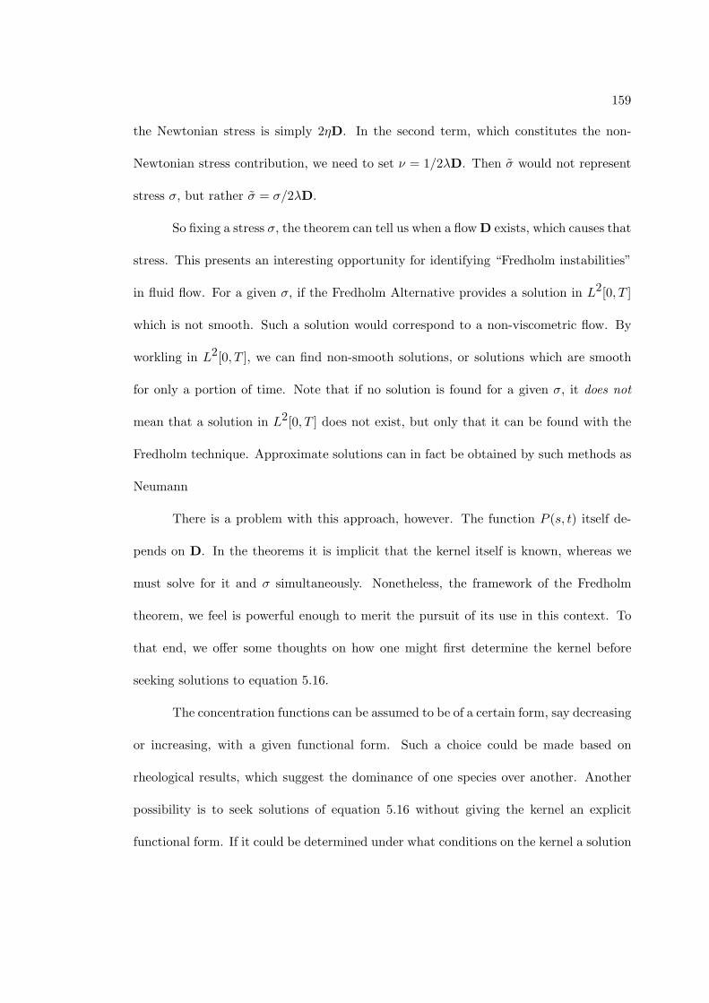
159

the Newtonian stress is simply 2ηD. In the second term, which constitutes the non-

Newtonian stress contribution, we need to set ν = 1/2λD. Then σ would not represent

stress σ, but rather σ = σ/2λD.

So fixing a stress σ, the theorem can tell us when a flow D exists, which causes that

stress. This presents an interesting opportunity for identifying “Fredholm instabilities”

in fluid flow. For a given σ, if the Fredholm Alternative provides a solution in L2[0, T ]

which is not smooth. Such a solution would correspond to a non-viscometric flow. By

workling in L2[0, T ], we can find non-smooth solutions, or solutions which are smooth

for only a portion of time. Note that if no solution is found for a given σ, it does not

mean that a solution in L2[0, T ] does not exist, but only that it can be found with the

Fredholm technique. Approximate solutions can in fact be obtained by such methods as

Neumann

There is a problem with this approach, however. The function P (s, t) itself de-

pends on D. In the theorems it is implicit that the kernel itself is known, whereas we

must solve for it and σ simultaneously. Nonetheless, the framework of the Fredholm

theorem, we feel is powerful enough to merit the pursuit of its use in this context. To

that end, we offer some thoughts on how one might first determine the kernel before

seeking solutions to equation 5.16.

The concentration functions can be assumed to be of a certain form, say decreasing

or increasing, with a given functional form. Such a choice could be made based on

rheological results, which suggest the dominance of one species over another. Another

possibility is to seek solutions of equation 5.16 without giving the kernel an explicit

functional form. If it could be determined under what conditions on the kernel a solution

160

would or would not exist, this itself would be a useful result. Our view is that the

theory of integral equations should at least be considered in obtaining information on

the predictions of any integral model. We have started along that path and shown not

only how to connect the Fredholm theorem to our constitutive equation 5.13, but that

our replacement function P (s, t) has the necessary properties to implement the theory.

161

Chapter 6

Directions for future research

Both experimental observations on wormlike micellar fluids and a mathematical

description of the fluid flow have been considered. Experimentally we have observed

shear thickening in dilute solutions of equimolar CPCl/NaSal. In the semi-dilute regime,

there is a again a thickening range of shear rates, but at lower shear rates in the semi-

dilute range, the fluids shear thin. It is well established that the thickening in dilute

solutions is due to the formation of SIS, though the mechanism of this formation is

not understood. Studying the thickening process for dilute and semi-dilute fluids may

give insight to this process. The fluids that shear thin probably consist of longer, more

flexible micelles than the dilute fluids, so if it could be determined wether SIS form in

the thickening range of shear rates, such factors as inception time for growth, maximum

viscosity reached and magnitude of fluctuations could be correlated with micellar length.

This could prove very helpful in understanding the processes leading to SIS formation.

The dependence of thickening and SIS formation on micellar length could also be studied

through temperature.

We have presented data suggesting that the micellar scission reactions in equimo-

lar solutions of CPCl/NaSal are in the “slow-breaking” regime. A natural question to

ask is whether SIS form in the “fast-breaking” limit, and if so how they compare to those

formed in equimolar CPCl/NaSal. We have also suggested that SIS play a role in the

162

oscillations of a rising bubble in equimolar CPCl/NaSal, and we saw that bubbles do not

oscillate in the fluids we tested which are in the “fast-breaking” limit. The dependence

of SIS formation on the micellar scission rates would also provide information about the

oscillatory instability in rising air bubbles.

The formation of SIS or “bundles” is central to the experiments in rheology and

rising bubbles, but it also plays a role in our model. The prediction of shear thickening

was made by the 2-species (Figure 4.6) model which excluded bundle formation, but it

failed to predict a subsequent thinning. With the inclusion of the bundle population

b(t), the model was able to capture shear thickening followed by shear thining (Figure

4.10). What we would like to see in our model, is a predicted rheology which shows a

zero shear plateau, shear thinning, a modest shear thickening followed by thining again,

as for 7 mM CPCl/NaSal in Figure 2.7. A better understanding of SIS formation could

lead to such a prediction for the model. The model parameters in the ODE’s 4.20-4.22

could then be chosen to represent what experiments suggest are responsible for observed

rheology.

The integral equation 5.13 offers a variety of directions for future research. The

application of Fredholm theory could be explored to answer fundamental questions on

the predictions of the model. Assuming functional forms for the concentration functions

to determine the replacement functions P aµ

, P bµ

, and P cµ

, one can seek solutions D to

prescribed stresses σ(t). As we mentioned in Chapter 5, it would be interesting to see

solutions which have singularities. It may be possible to find approximate solutions

through the use of Neumann iterates.

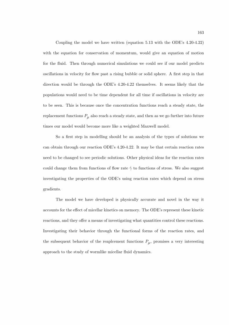
163

Coupling the model we have written (equation 5.13 with the ODE’s 4.20-4.22)

with the equation for conservation of momentum, would give an equation of motion

for the fluid. Then through numerical simulations we could see if our model predicts

oscillations in velocity for flow past a rising bubble or solid sphere. A first step in that

direction would be through the ODE’s 4.20-4.22 themselves. It seems likely that the

populations would need to be time dependent for all time if oscillations in velocity are

to be seen. This is because once the concentration functions reach a steady state, the

replacement functions Pµ also reach a steady state, and then as we go further into future

times our model would become more like a weighted Maxwell model.

So a first step in modelling should be an analysis of the types of solutions we

can obtain through our reaction ODE’s 4.20-4.22. It may be that certain reaction rates

need to be changed to see periodic solutions. Other physical ideas for the reaction rates

could change them from functions of flow rate γ to functions of stress. We also suggest

investigating the properties of the ODE’s using reaction rates which depend on stress

gradients.

The model we have developed is physically accurate and novel in the way it

accounts for the effect of micellar kinetics on memory. The ODE’s represent these kinetic

reactions, and they offer a means of investigating what quantities control these reactions.

Investigating their behavior through the functional forms of the reaction rates, and

the subsequent behavior of the reaplcement functions Pµ, promises a very interesting

approach to the study of wormlike micellar fluid dynamics.

164

References

[1] L. Pauling, General Chemistry, 3rd edition, (W. H. Freeman, San Francisco, 1970).

[2] J. Israelachvili, Intermolecular and Surface Forces, 2nd edition, (Academic Press,

New York, 1991).

[3] R. G. Larson, The Structure and Rheology of Complex Fluids

[4] Micelles, Membranes, Microemulsions, and Monolayers, W. Gelbart, et al., editors,

(Springer, New York, 1994).

[5] A. Ben-Shaul & W. Gelbart, in [4].

[6] H. Rehage & H. Hoffmann, Rheological Properties of Viscoelastic Surfactant Sys-

tems. J. Phys. Chem. 92, 4712 (1988).

[7] Z. Lin, J. J. Cai, L. E. Scriven, & H. T. Davis, Spherical to Wormlike Micelle

Transition in CTAB Solutions, J. Phys. Chem 98, 5984 (1994).

[8] I. A. Kadoma, C. Ylitalo, & J. W. van Egmond, Structural Tranisitions in Wormlike

Micelles, Rheol. Acta 36, 1 (1997).

[9] M. E. Cates & S. Candau, Statics and Dynamics of Worm-Like Surfactant Micelles.

J. Phys.: Condens. Matter 2, 6869 (1990).

[10] J. Appell, G. Porte, A. Khatory, F. Kern, & S. Candau, Static and Dynamic Prop-

erties of a Network of Wormlike Surfactant Micelles (CetylPyridinium Chlorate in

Sodium-Chlorate Brine). J. de Physique II 2, 1045 (1992).

165

[11] H. Rehage & H. Hoffmann, Viscoelastic Surfactant Solutions - Model Systems for

Rheological Research. Molecular Physics 74, 933 (1991).

[12] V. Hartmann & R. Cressely, Shear Thickening of an Aqueous Micellar Solution of

Cetyltrimethylammonium Bromide and Sodium Tosylate, J. Phys. II France 7, 1087

(1997).

[13] V. Degiorgio & M. Corti, in Physics of Amphiphiles: Micelles, Vesicles, and Mi-

croemulsions, (Elsevier, New York, 1985).

[14] T. Shikata, H. Hirata, E. Takatori, & K Osaki, Nonlinear Viscoelastic Behavior of

Aqueous Detergent Solutions. J. Non-Newtonian Fluid Mech. 28, 171 (1988).

[15] C. Grand, J. Arrault, & M. E. Cates, Slow Transients and Metastability in Wormlike

Micellar Rheology. J. de Physique II 7, 1071 (1997).

[16] S. Lerouge, J-P. Decruppe, J-F. Berret, Correlations Between Rheological and Op-

tical Properties of a Micellar Solution Under Shear Banding Flow. Langmuir 16,

6464 (2000).

[17] C. Liu & D. Pine, Shear-Induced Gelation and Fracture in Micellar Solutions. Phys.

Rev. Lett. 77, 2121 (1996).

[18] L. Smolka & A. Belmonte, Drop Pinch-Off and Filament Dynamics of Wormlike

Micellar Fluids. J. Non-Newtonian Fluid Mech. 115, 1 (2003).

[19] A. Belmonte, Self-Oscillations of a Cusped Bubble Rising Through a Micellar Solu-

tion. Rheol. Acta 39, 554 (2000).

166

[20] A. Jayaraman & A. Belmonte, Oscillations of a Solid Sphere Falling Through a

Wormlike Micellar Fluid. Phys. Rev. E 67, 65301 (2003).

[21] J. Rothstein, Transient Extensional Rheology of Wormlike Micellar Solutions. J.

Rheol. 47, 1227 (2003).

[22] Y. Liu, T. Liao, & D. Joseph, A Two-Dimensional Cusp at the Trailing Edge of an

Air Bubble Rising in a Viscoelastic Liquid. J. Fluid Mech. 304, 321 (1995).

[23] A. Mollinger, E. Cornelissen, & B. van den Brule, An Unexpected Phenomenon

Observed in Particle Settling: Oscillating Falling Spheres. J. Non-Newtonian Fluid

Mech. 86, 389 (1999).

[24] P. Weidman, B. Roberts, & S. Eisen, Progress in Nonlinear Science, Proceedings

III, V.D. Shalfeev ed., (Nizhny Novgorod, 2002), 103.

[25] M. In, G. Warr, & R. Zana, Dynamics of Branched Threadlike Micelles. Phys. Rev.

Lett. 83, 2278 (1999).

[26] V. Schmitt, F. Lequeux, A. Pousse, & D. Roux, Flow Behavior and Shear Induced

Transition Near an Isotropic-Nematic Transition in Equilibrium Polymers. Langmuir

10, 955 (1994).

[27] R. Hartunian & W. Sears, J. Fluid Mech. 3, 27 (1957).

[28] D. Rodrigue, D. De Kee, & C. Chan Man Fong, An Experimental Study of the

Effect of Surfactants on the Free Rise Velocity of Gas Bubbles. J. Non-Newtonian

Fluid Mech. 66, 213 (1996).

167

[29] S. Candau, A. Khatory, F. Lequeux, & F. Kern, Rheological Behavior of Wormlike

Micelles - Effect of Salt Content. J. de Physique IV 3, 197 (1993).

[30] J.-F. Berret, Transient Rheology of Wormlike Micelles. Langmuir 13, 2227 (1997).

[31] T. Drye & M. E. Cates, Living Networks - The Role of Cross-Links in Entangled

Surfactant Solutions. J. Chem. Phys. 96, 1367 (1992).

[32] P. Pincus, Phase Tranisitions - Y’s and Ends. Science 290, 1307 (2000).

[33] F. Lequeux & S. Candau, in [46].

[34] G. Fuller, Optical Rheometry. Ann. Rev. Fluid Mech. 22, 387 (1990).

[35] Y. Hu, S. Wang, & A. Jamieson, Rheological and Flow Birefringence Studies of a

Shear Thickening Complex Fluid - a Surfactant Model System. J. Rheol. 37, 531

(1993).

[36] S. Chen & J. P. Rothstein, Flow of a Wormlike Micellar System Past a Falling

Sphere. J. Non-Newtonian Fluid Mech. 116, 205 (2004).

[37] S. Kwon & M. Kim, Topological Transition in Aqueous Micellar Solutions. Phys.

Rev. Lett. 89, 258302 (2002).

[38] P. Boltenhagen, Y. Hu, E. Matthys, & D. Pine, Inhomogenous Structure Formation

and Shear Thickening in Worm-Like Micellar Solutions. Europhys. Lett. 38, 389

(1997).

168

[39] S. Keller, P. Boltenhagen, D. Pine, & J. Zasadzinski, Direct Observation of Shear

Induced Structures in Wormlike Micellar Solutions by Freeze Fracture Electron Mi-

croscopy. Phys. Rev. Lett. 80, 2725 (1998).

[40] E. Wheeler, P. Fischer, & G. Fuller, Time-Periodic Flow Induced Structures and

Instabilites in a Viscoelastic Surfactant Solution. J. Non-Newtonian Fluid Mech.

75, 193 (1998).

[41] P. Fischer, Time Dependent Flow in Equimolar Micellar Solutions: Transient Be-

haviour of the Shear Stress and First Normal Stress Difference in Shear Induced

Structures Coupled with Flow Instabilites. Rheol. Acta 39, 234 (2000).

[42] J.-F. Berret, J. Appell, & G. Porte, Linear Rheology of Entangled Wormlike Mi-

celles. Langmuir 9, 2851 (1993).

[43] J.-F. Berret, D. C. Roux, & G. Porte, Isotropic-to-Nematic Transition in Wormlike

Micelles Under Shear. J. de Physique II 4, 1261 (1994).

[44] R. Granek & M. E. Cates, Stress Relaxation in Living Polymers-Results from a

Poisson Renewal Model. J. Chem. Phys. 96, 4758 (1992).

[45] A. Khatory, F. Lequeux, F. Kern, & S. J. Candau, Linear and Nonlinear Viscoelas-

ticity of Semidilute Solutions of Wormilike Micelles at High Salt Content. Langmuir

9, 1456 (1993).

[46] Theoretical Challenges in the Dynamics of Complex Fluids, T. McLeish, ed.,

(Kluwer, Boston, 1997)

169

[47] R. B. Bird, R. C. Armstrong, & O. Hassager, Dynamics of Polymeric Liquids, 2nd

ed. (Wiley, New York, 1987), vol. 1.

[48] James Clerk Maxwell, On the Dynamical Theory of Gasses. Phil. Trans. Roy. Soc.

A157, 49 (1867).

[49] H. Rehage & H. Hoffmann, Viscoelastic Detergent Solutions. Faraday Discuss.

Chem. Soc. 76, 363 (1983).

[50] M. E. Cates, Reptation of Living Polymers - Dynamics of Entangled Polymers in

the Presence of Reversible Chain-Scission. Macromolecules 20, 2289 (1987).

[51] M. E. Cates, Nonlinear Viscoelasticity of Wormlike Micelles. J. Phys. Chem. 94,

371 (1990).

[52] F. Lequeux, Linear Response of Self Assembling Systems - Mean Field Solution. J.

de Physique II 1, 195 (1991).

[53] O. Manero, F. Bautista, J. F. A. Soltero, & J. E. Puig, Dynamics of Wormlike

Micelles: The Cox-Merz Rule. J. Non-Newtonian Fluid Mech. 106, 1 (2002).

[54] E. Cappelaere, J.-F. Berret, J.-P. Decruppe, R. Cressely, & P. Lindner, Rheology,

Birefringence, and Small Angle Neutron Scattering in a Charged Micellar System:

Evidence of a Shear Induced Phase Transition. Phys. Rev. E 56, 1869 (1997).

[55] V. Schmitt, C. M. Marques, & F. Lequeux, Shear - Induced Phase-Separation of

Complex Fluids-The Role of Flow Concentration Coupling. Phys. Rev. E 52, 4009

(1995).

170

[56] B. H. A. A. van den Brule & P. J. Hoogerbrugge, Brownian Dynamics Simulation

of Reversible Polymeric Networks. J. Non-Netonian Fluid Mech. 60, 303 (1995).

[57] J. Intae, Existence of Gelling Solutions for Coagulation-Fragmentation Equations.

Comm. Math. Phys. 194, 541 (1998).

[58] A. Vaccaro & G. Marrucci, A Model for the Nonlinear Rheology of Associating

Polymers. J. Non-Newtonian Fluid Mech. 92, 261 (2000).

[59] J. L. Goveas & P. D. Olmsted, A Minimal Model for Vorticity and Gradient Banding

in Complex Fluids. Eur. Phys. J. E 6, 79 (2001).

[60] R. Bruinsma, W. Gelbart, & A. Ben-Shaul, Flow-Induced Gelation of Living (Mi-

cellar) Polymers. J. Chem. Phys. 96, 15 (1992).

[61] H. Paine, Koll. Z 11, 2115 (1912).

[62] M. von Smoluchowski, Z. Phys. Chem. 112, 1 (1916).

[63] M. Doi & S. F. Edwards, The Theory of Polymer Dynamics, (Oxford University

Press, New York, 1986).

[64] M. S. Turner & M. E. Cates, The Relaxation Spectrum of Polymer Length Distri-

butions. J. Phys. France 51, 307 (1990).

[65] C. M. Marques & M. E. Cates, Nonlinear Thermodynamic Relaxation in Living

Polymer Systems. J. Phys. II 1, 489 (1991).

[66] M. E. Cates & M. S. Turner, Flow-Induced Gelation of Rodlike Micelles. Europhys.

Lett. 11, 681 (1990).

171

[67] F. Bautista, J. F. A. Soltero, J. H. Perez-Lopez, J. E. Puig, & O. Manero, On

the Shear Banding Flow of Elongated Micellar Solutions. J. Non-Newtonian Fluid

Mech. 94, 57 (2000).

[68] J. D. Ferry, Viscoelastic Properties of Polymers, (Wiley, New York, 1980).

[69] J. F. A. Soltero, J. E. Puig, O. Manero, Rheology of the CetyltrimethylAmmonium

Tosilate-Water System.2. Linear Viscoelastic Regime. Langmuir 12, 2654 (1996).

[70] J. F. A. Soltero, F. Bautista, J. E. Puig, O. Manero, Rheology of CetyltrimethylAm-

monium p-Toluenesulfonate-Water System.3. Nonlinear Viscoelasticity. Langmuir

15, 1604 (1999).

[71] D. Acierno, F. P. La Mantia, G. Marucci, G. Titomanlio, J. Non-Newtonian Fluid

Mech. 1, 125 (1976).

[72] H. R. Warner Jr., IE & C Fundam. 11, 379 (1972).

[73] H. A. Stone, Dynamics of Drop Deformation and Breakup in Viscous Fluids. Annual

Review of Fluid Mechanics 26, 65 (1994).

[74] A. Prosperetti, Bubbles. Phys. Fluids 16, 1852 (2004).

[75] O. Hassager, Nature 279, 402 (1979).

[76] N. Z. Handzy & A. Belmonte, Oscillatory Rise of Bubbles in Wormlike Micellar

Fluids with Different Microstructures. Phys. Rev. Lett. 92, 124501 (2204).

[77] M. Renardy, Mathematical Analysis of Viscoelastic Flows, (Society for Industrial

and Applied Mathematics, Philadelphia, 2000).

172

[78] G. K. Batchelor, An Introduction to Fluid Dynamics, (Cambridge University Press,

Cambridge, 1967).

[79] M. D. Chilcott & J. M. Rallison, Creeping Flow of Dilute Polymer Solutions Past

Cylinders and Spheres. J. Non-Newtonian Fluid Mech. 29, 381 (1988).

[80] L. E. Wedgewood, D. N. Ostrov, & R. B. Bird, A Finitely Extensible Bead-Spring

Chain Model for Dilute Polymer Solutions. J. Non-Newtonian Fluid Mech. 40, 119

(1991).

[81] N. A. Spenley, M. E. Cates, & T. C. B. McLeish, Nonlinear Rheology of Wormlike

Micelles. Phys. Rev. Lett. 71, 939 (1993).

[82] F. Reif, Fundamentals of Statistical and Thermal Physics, (McGraw-Hill, New York,

1965).

[83] R. I. Tanner, Engineering Rheology, (Oxford University Press, New York, 1985).

[84] R. Gamez-Corrales, J.-F. Berret, L. M. Walker, & J. Oberdisse, Shear Thicken-

ing Dilute Surfactant Solutions: Equilibrium Structure as Studied by Small-Angle

Neutron Scattering. Langmuir 15, 6755 (1999).

[85] G. Porte, J.-F. Berret, & J. L. Harden, Inhomogeneous Flows of Complex Fluids:

Mechanical Instability versus Non-Equilibrium Phase Transition, J. Phys. II 7, 459

(1997).

[86] O. Radulescu & P. D. Olmsted, Matched Asymptotic Solutions for the Steady

Banded Flow of the Diffusive Johnson-Segalman Model in Various Geometries, J.

Non-Newtonian Fluid Mech. 91, 143 (2000).

173

[87] J. P. Keener, Principles of Applied Mathematics, (Perseus Books, Reading, Mas-

sachusetts, 1988).

[88] F. Riesz & B. Sz.-Nagy, Functional Analysis, (Dover Publications, New York, 1990).

Vita

Nestor Zenon Handzy was born to Jerry Nestor Handzy and Alexandra Ann

Handzy, in New York City. He received a B.A. in mathematics with a minor in physics

from the University of Pennsylvania in Philadelphia. After receiving his Ph.D. in math-

ematics from The Pennsylvania State University, he will work in the Department of

Complex Systems at The Weizmann Institute in Rehovot, Israel. American by birth,

Nestor’s ancestry is Ukrainian, and he appreciates and enjoys his Ukrainian heritage

through language, arts, history, and religion.