Explicit Approaches to Elliptic Curves

and Modular Forms

William Stein

Associate Professor of Mathematics

University of California, San Diego

Math 168a: 2005-09-26

1

Outline of Course and this Lecture

1. Pythagoras and Fermat

2. Mordell-Weil Groups and the BSD Conjecture

3. Modularity of Elliptic Curves

4. Computing Modular Forms

2

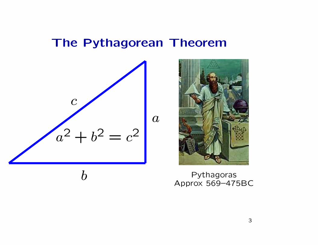
The Pythagorean Theorem

a2 + b2 = c2

ca

b PythagorasApprox 569–475BC

3

Pythagorean Triples

Triples of integers a, b, c such that

a2 + b2 = c2

(3,4,5)(5,12,13)(7,24,25)(9,40,41)(11,60,61)(13,84,85)(15,8,17)(21,20,29)(33,56,65)(35,12,37)(39,80,89)(45,28,53)(55,48,73)(63,16,65)(65,72,97)(77,36,85)...

4

Enumerating Pythagorean Triples

(−1,0)

(0, t)

(x, y) Slope = t =y

x + 1

x =1 − t2

1 + t2

y =2t

1 + t2

If t = rs, then a = s2 − r2, b = 2rs, c = s2 + r2

is a Pythagorean triple, and all primitive unordered triplesarise in this way.

5

Fermat’s “Last Theorem”

No analogue of “Pythagorean triples” with exponent 3 or higher.

6

Wiles’s Proof of FLT Uses Elliptic Curves

An elliptic curve is a nonsingular plane cubic curvewith a rational point (possibly “at infinity”).

-2 -1 0 1 2-3

-2

-1

0

1

2

∞

x

y

y2 + y = x3 − x

EXAMPLES

y2 + y = x3 − x

x3 + y3 = 1 (Fermat cubic)

y2 = x3 + ax + b

3x3 + 4y3 + 5 = 0

7

The Frey Elliptic Curve

Suppose Fermat’s conjecture is FALSE. Then there is a prime

ℓ ≥ 5 and coprime positive integers a, b, c with aℓ + bℓ = cℓ.

Consider the corresponding Frey elliptic curve:

y2 = x(x − aℓ)(x + bℓ).

Ribet’s Theorem: This elliptic curve is not modular.

Wiles’s Theorem: This elliptic curve is modular.

Conclusion: Fermat’s conjecture is true.

8

The Group Operation

-2 -1 0 1 2 3-5

-4

-3

-2

-1

0

1

2

3

4

x

y

y2 + y = x3 − x

∞Point at infinity

⊕ =

(−1,0) ⊕ (0,−1) = (2,2)

The set of points

on E forms an abelian group.

9

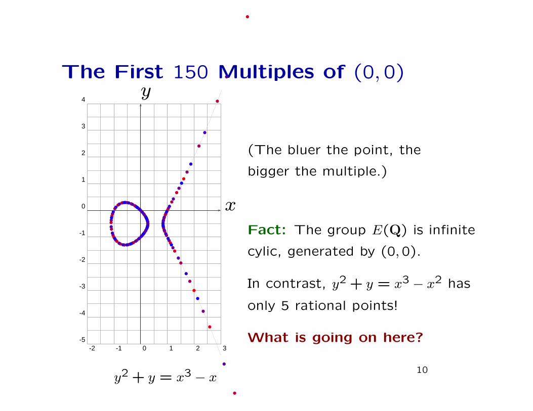
The First 150 Multiples of (0,0)

(The bluer the point, the

bigger the multiple.)

Fact: The group E(Q) is infinite

cylic, generated by (0,0).

In contrast, y2 + y = x3 − x2 has

only 5 rational points!

What is going on here?-2 -1 0 1 2 3

-5

-4

-3

-2

-1

0

1

2

3

4

x

y

y2 + y = x3 − x10

Mordell’s Theorem

Theorem (Mordell). The group E(Q) of rational points on an

elliptic curve is a finitely generated abelian group, so

E(Q) ∼= Zr ⊕ T,

with T = E(Q)tor finite.

Mazur classified the possibilities for T . It is conjectured that r

can be arbitrary, but the biggest r ever found is (probably) 24.

11

The Simplest Solution

Can Be Huge

Simplest solution to y2 = x3 + 7823:

x =2263582143321421502100209233517777

143560497706190989485475151904721

y =186398152584623305624837551485596770028144776655756

1720094998106353355821008525938727950159777043481

(Found by Michael Stoll in 2002.)

12

The Central Question

Given an elliptic curve E,

what is the rank of E(Q)?

13

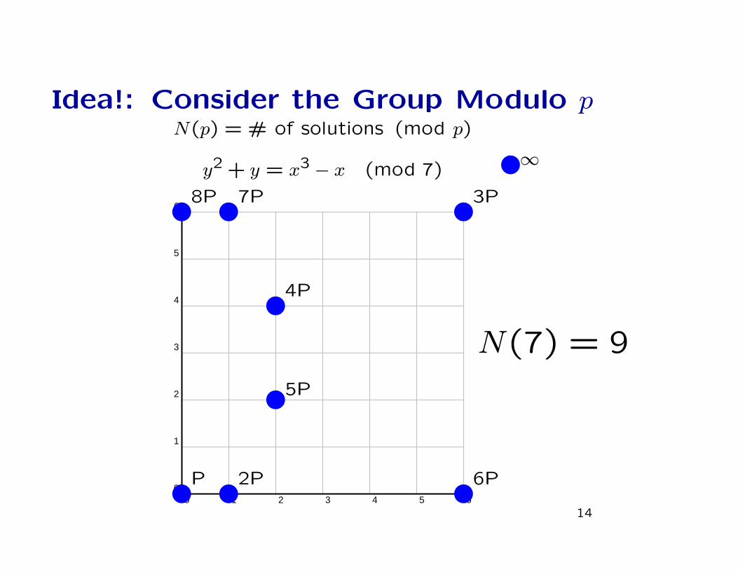
Idea!: Consider the Group Modulo pN(p) = # of solutions (mod p)

y2 + y = x3 − x (mod 7)

0 1 2 3 4 5 60

1

2

3

4

5

6

5P

P 6P2P

7P 3P8P

4P

∞

N(7) = 9

14

Counting Points

Cambridge EDSAC: The first

point counting supercomputer...

Birch and Swinnerton-Dyer

15

Hecke Eigenvalues

Hasse

Let

ap = p + 1 − N(p).

Hasse proved that

|ap| ≤ 2√

p.For y2 + y = x3 − x:

a2 = −2, a3 = −3, a5 = −2, a7 = −1, a11 = −5, a13 = −2,

a17 = 0, a19 = 0, a23 = 2, a29 = 6, . . .

16

Birch and Swinnerton-Dyer

17

The L-Function

Theorem (Wiles et al., Hecke) The following function extends

to a holomorphic function on the whole complex plane:

L∗(E, s) =∏

p∆

1

1 − ap · p−s + p · p−2s

.

Here ap = p + 1 − #E(Fp) for all p∆E. Note that formally,

L∗(E,1) =∏

p∆

(

1

1 − ap · p−1 + p · p−2

)

=∏

p∆

(

p

p − ap + 1

)

=∏

p∆

p

Np

Standard extension to L(E, s) at bad primes.

18

Real Graph of the L-Series of

y2 + y = x3 − x

19

More Graphs of Elliptic Curve

L-functions

20

Absolute Value of L-series on Complex

Plane for y2 + y = x3 − x0 0 . 5 1 1 . 5 2 2 . 5 3 3 . 5 4� 0 . 4

� 0 . 20

0 . 20 . 4

21

Conjectures Proliferated

“The subject of this lecture is rather a special one. I want to de-

scribe some computations undertaken by myself and Swinnerton-

Dyer on EDSAC, by which we have calculated the zeta-functions

of certain elliptic curves. As a result of these computations we

have found an analogue for an elliptic curve of the Tamagawa

number of an algebraic group; and conjectures have proliferated.

[...] though the associated theory is both abstract and technically

complicated, the objects about which I intend to talk are usually

simply defined and often machine computable; experimentally

we have detected certain relations between different in-

variants, but we have been unable to approach proofs of these

relations, which must lie very deep.” – Birch 1965

22

The Birch and Swinnerton-Dyer

Conjecture

Conjecture: Let E be any elliptic curve over Q. The order of

vanishing of L(E, s) as s = 1 equals the rank of E(Q).

23

The Kolyvagin and Gross-Zagier

Theorem

Theorem: If the ordering of vanishing ords=1L(E, s) is ≤ 1, then

the conjecture is true for E.

24

Elliptic Curves are “Modular”

An elliptic curve is modular if the numbers ap are coefficients of

a “modular form”. Equivalently, if L(E, s) extends to a complex

analytic function on C (with functional equation).

Theorem (Wiles et al.): Every elliptic curve over the rational

numbers is modular.

Wiles at the Institute for Advanced Study

25

Modular Forms

The definition of modular forms as holomorphic functions satis-

fying a certain equation is very abstract.

For today, I will skip the abstract definition, and instead give you

an explicit “engineer’s recipe” for producing modular forms. In

the meantime, here’s a picture:

26

Computing Modular Forms: Motivation

Motivation: Data about modular forms is extremely useful to

many research mathematicians (e.g., number theorists, cryptog-

raphers). This data is like the astronomer’s telescope images.

One of my longterm research goals is to compute modular forms

on a huge scale, and make the resulting database widely

available. I have done this on a smaller scale during the last 5

years — see http://modular.ucsd.edu/Tables/

27

What to Compute: Newforms

For each positive integer N there is a finite list of newforms of

level N . E.g., for N = 37 the newforms are

f1 = q − 2q2 − 3q3 + 2q4 − 2q5 + 6q6 − q7 + · · ·f2 = q + q3 − 2q4 − q7 + · · · ,

where q = e2πiz.

The newforms of level N determine all the modular forms of

level N (like a basis in linear algebra). The coefficients are alge-

braic integers. Goal: compute these newforms.

Bad idea – write down many elliptic curves and compute the numbers ap

by counting points over finite fields. No good – this misses most of the

interesting newforms, and gets newforms of all kinds of random levels, but

you don’t know if you get everything of a given level.

28

An Engineer’s Recipe for Newforms

Fix our positive integer N . For simplicity assume that N is prime.

1. Form the N + 1 dimensional Q-vector space V with basis the symbols[0], . . . , [N − 1], [∞].

2. Let R be the suspace of V spanned by the following vectors, forx = 0, . . . , N−1,∞:

[x] − [N − x]

[x] + [x.S]

[x] + [x.T ] + [x.T 2]

S =(

0 −11 0

)

, T =(

0 −11 −1

)

, and x.(

a bc d

)

= (ax + c)/(bx + d).

3. Compute the quotient vector space M = V/R. This involves “intelligent”sparse Gauss elimination on a matrix with N + 1 columns.

29

4. Compute the matrix T2 on M given by

[x] 7→ [x. ( 1 00 2 )] + [x. ( 2 0

0 1 )] + [x. ( 2 10 1 )] + [x. ( 1 0

1 2 )].

This matrix is unfortunately not sparse. Similar recipe for matrices Tn

for any n.

5. Compute the characteristic polynomial f of T2.

6. Factor f =∏

gei

i . Assume all ei = 1 (if not, use a random linear combi-nation of the Tn.)

7. Compute the kernels Ki = ker(gi(T2)). The eigenvalues of T3, T5, etc.,acting on an eigenvector in Ki give the coefficients ap of the newformsof level N .

Implementation

• I implemented code for computing modular forms that’s in-

cluded with MAGMA (non-free, closed source):

http://magma.maths.usyd.edu.au/magma/.

• I want something better, so I’m implementing modular sym-

bols algorithms as part of SAGE:

http://modular.ucsd.edu/sage/.

• I’m finishing a book on these algorithms that will be pub-

lished by the American Mathematical Society.

30

The Modular Forms Database Project

• Create a database of all newforms of level N for each N < 100000. Thiswill require many gigabytes to store. (50GB?)

• So far this has only been done for N < 7000 (and is incomplete), so100000 is a major challenge.

• Involves sparse linear algebra over Q on spaces of dimension up to 200000and dense linear algebra on spaces of dimension up to 25000.

• Easy to parallelize – run one process for each N .

• Will be very useful to number theorists and cryptographers.

• John Cremona has done something similar but only for the newformscorresponding to elliptic curves (he’s at around 120000 right now), sothis should be do-able.

31

Goals for Math 168

• [Elliptic Curves] Definition, group structure, applications

to cryptography, L-series, the Birch and Swinnerton-Dyer

conjecture (a million dollar Clay Math prize problem).

• [Modular Forms] Definition (of modular forms of weight

2), connection with elliptic curves and Andrew Wiles’s cele-

brated proof of Fermat’s Last Theorem, how to use modular

symbols to compute modular forms.

• [Research] Get everyone in 168a involved in some aspect of

my research program: algorithms needed for SAGE, making

data available online, efficient linear algebra, etc.

32